Embed Size (px)
Citation preview
Decisions Under Risk– Mathematics in Action –
Tim C. Adams, ASQ CRE
NASA Kennedy Space Center
Engineering Directorate
American Mathematical Association of Two-Year Colleges
44th Annual Conference
November 15, 2018 (revised)
Presentation Objectives
Demonstrate the benefit of Mathematics in the work place.
“Where is this stuff ever used?”
“Did it really help?”
Provide real examples (questions) where the NASA
program/project manager was faced with making a decision
involving technical risk with uncertainty.
Provide insights on how a Reliability-Risk Engineer responded to
these questions (problems).
Observe when the probabilistic method (as opposed to
deterministic method) was and was not used.
1

Thinking Styles and Belief Systems
Big Q vs. Little q
• Qualitative (expert opinion) vs. quantitative (mathematical analysis)
• Determinism (certain) vs. Probabilism (uncertain)
Uncertainty does not imply no knowledge, but it does imply the
exact outcome is not completely predictable. Most observable
phenomena contain a certain amount of uncertainty.
“Basically, an anti-empirical system states that things may look
like X, but in reality they are Y. Between us and reality is a
screen of ideology.”“God and Mankind: Comparative Religions,” Robert Oden (former Professor and Chair, Department of Religion,
Dartmouth College), The Great Courses, Lecture 2, 1998
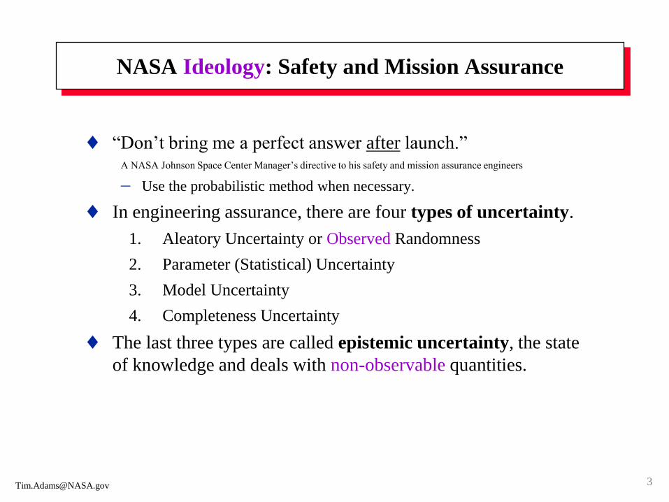
NASA Ideology: Safety and Mission Assurance
“Don’t bring me a perfect answer after launch.”A NASA Johnson Space Center Manager’s directive to his safety and mission assurance engineers
Use the probabilistic method when necessary.
In engineering assurance, there are four types of uncertainty.
1. Aleatory Uncertainty or Observed Randomness
2. Parameter (Statistical) Uncertainty
3. Model Uncertainty
4. Completeness Uncertainty
The last three types are called epistemic uncertainty, the state
of knowledge and deals with non-observable quantities.
3
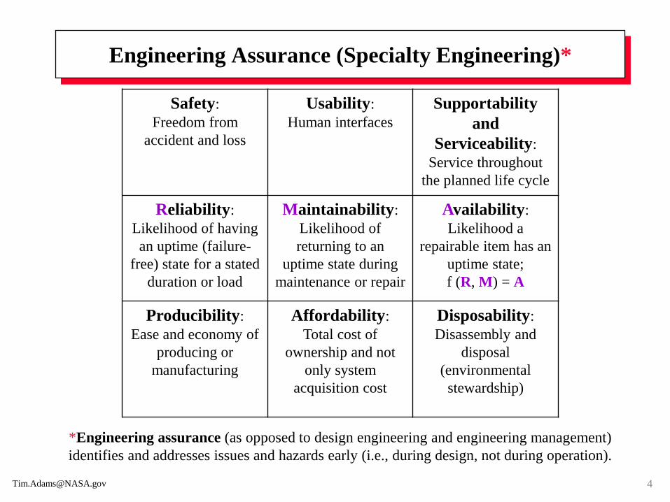
Engineering Assurance (Specialty Engineering)*
4
Safety:
Freedom from
accident and loss
Usability:
Human interfaces
Supportability
and
Serviceability:
Service throughout
the planned life cycle
Reliability:
Likelihood of having
an uptime (failure-
free) state for a stated
duration or load
Maintainability:
Likelihood of
returning to an
uptime state during
maintenance or repair
Availability:
Likelihood a
repairable item has an
uptime state;
f (R, M) = A
Producibility:
Ease and economy of
producing or
manufacturing
Affordability:
Total cost of
ownership and not
only system
acquisition cost
Disposability:
Disassembly and
disposal
(environmental
stewardship)
*Engineering assurance (as opposed to design engineering and engineering management)
identifies and addresses issues and hazards early (i.e., during design, not during operation).
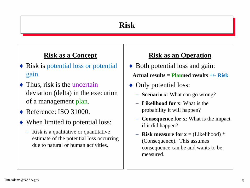
Risk
Risk as a Concept
Risk is potential loss or potential
gain.
Thus, risk is the uncertain
deviation (delta) in the execution
of a management plan.
Reference: ISO 31000.
When limited to potential loss:
Risk is a qualitative or quantitative
estimate of the potential loss occurring
due to natural or human activities.
Risk as an Operation
Both potential loss and gain:
Actual results = Planned results +/- Risk
Only potential loss:
Scenario x: What can go wrong?
Likelihood for x: What is the
probability it will happen?
Consequence for x: What is the impact
if it did happen?
Risk measure for x = (Likelihood) *
(Consequence). This assumes
consequence can be and wants to be
measured.
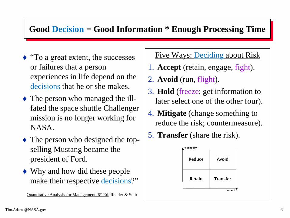
Good Decision = Good Information * Enough Processing Time
“To a great extent, the successes
or failures that a person
experiences in life depend on the
decisions that he or she makes.
The person who managed the ill-
fated the space shuttle Challenger
mission is no longer working for
NASA.
The person who designed the top-
selling Mustang became the
president of Ford.
Why and how did these people
make their respective decisions?”
Five Ways: Deciding about Risk
1. Accept (retain, engage, fight).
2. Avoid (run, flight).
3. Hold (freeze; get information to
later select one of the other four).
4. Mitigate (change something to
reduce the risk; countermeasure).
5. Transfer (share the risk).
Quantitative Analysis for Management, 6th Ed, Render & Stair
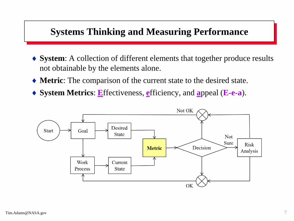
Systems Thinking and Measuring Performance
System: A collection of different elements that together produce results
not obtainable by the elements alone.
Metric: The comparison of the current state to the desired state.
System Metrics: Effectiveness, efficiency, and appeal (E-e-a).
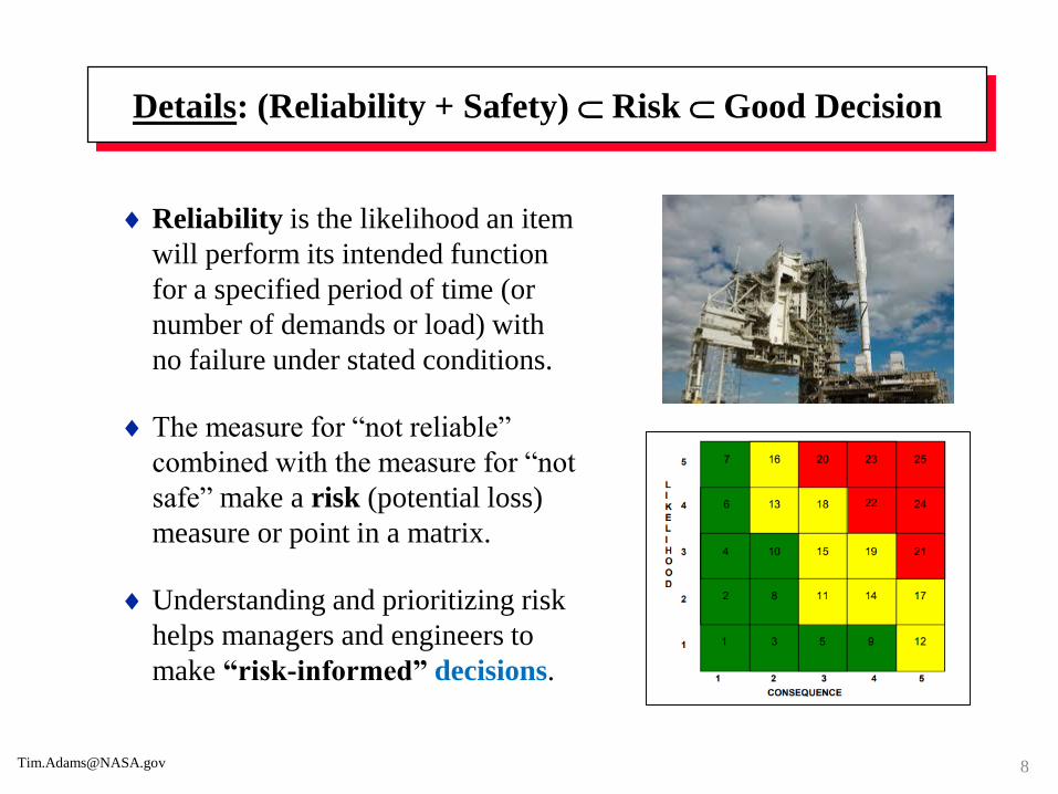
Details: (Reliability + Safety) Risk Good Decision
Reliability is the likelihood an item
will perform its intended function
for a specified period of time (or
number of demands or load) with
no failure under stated conditions.
The measure for “not reliable”
combined with the measure for “not
safe” make a risk (potential loss)
measure or point in a matrix.
Understanding and prioritizing risk
helps managers and engineers to
make “risk-informed” decisions.
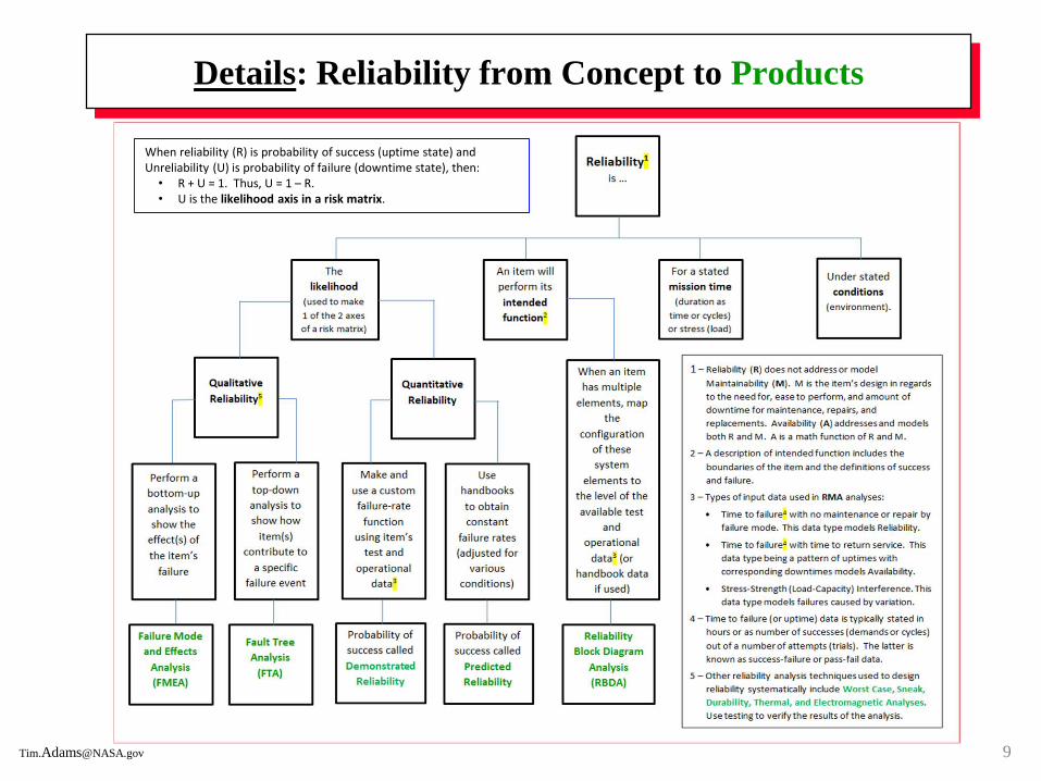
Details: Reliability from Concept to Products
When reliability (R) is probability of success (uptime state) and Unreliability (U) is probability of failure (downtime state), then:
• R + U = 1. Thus, U = 1 – R.• U is the likelihood axis in a risk matrix.
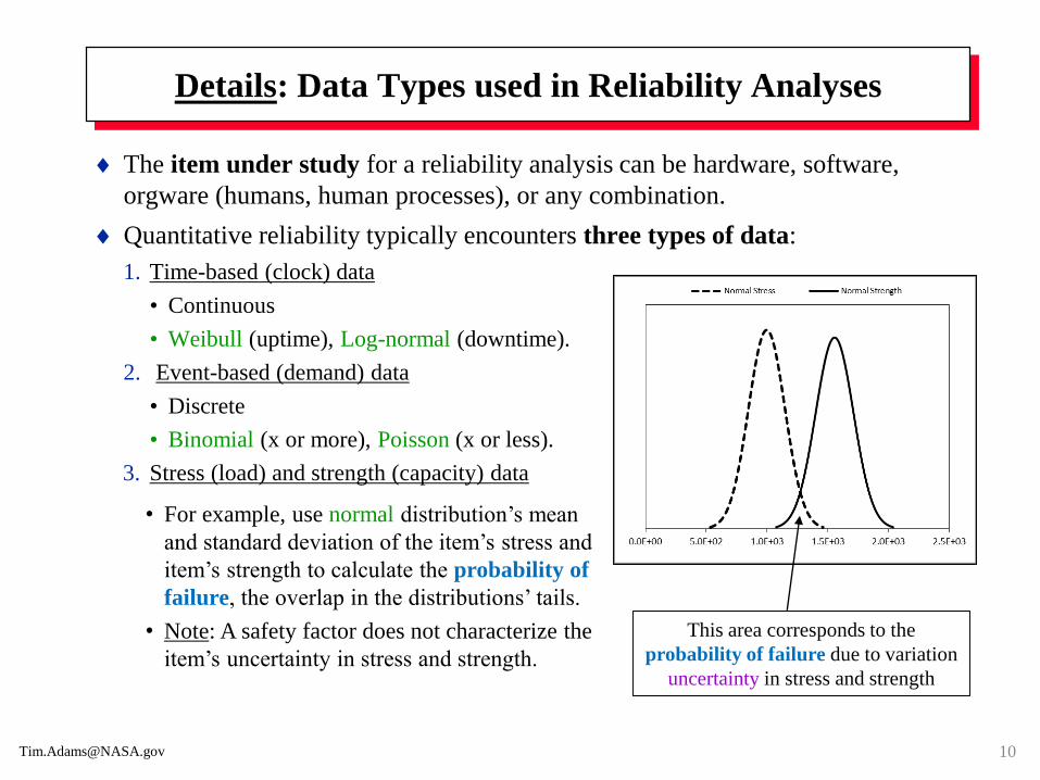
Details: Data Types used in Reliability Analyses
The item under study for a reliability analysis can be hardware, software,
orgware (humans, human processes), or any combination.
Quantitative reliability typically encounters three types of data:
1. Time-based (clock) data
• Continuous
• Weibull (uptime), Log-normal (downtime).
2. Event-based (demand) data
• Discrete
• Binomial (x or more), Poisson (x or less).
3. Stress (load) and strength (capacity) data
• For example, use normal distribution’s mean
and standard deviation of the item’s stress and
item’s strength to calculate the probability of
failure, the overlap in the distributions’ tails.
• Note: A safety factor does not characterize the
item’s uncertainty in stress and strength.
This area corresponds to the
probability of failure due to variation
uncertainty in stress and strength
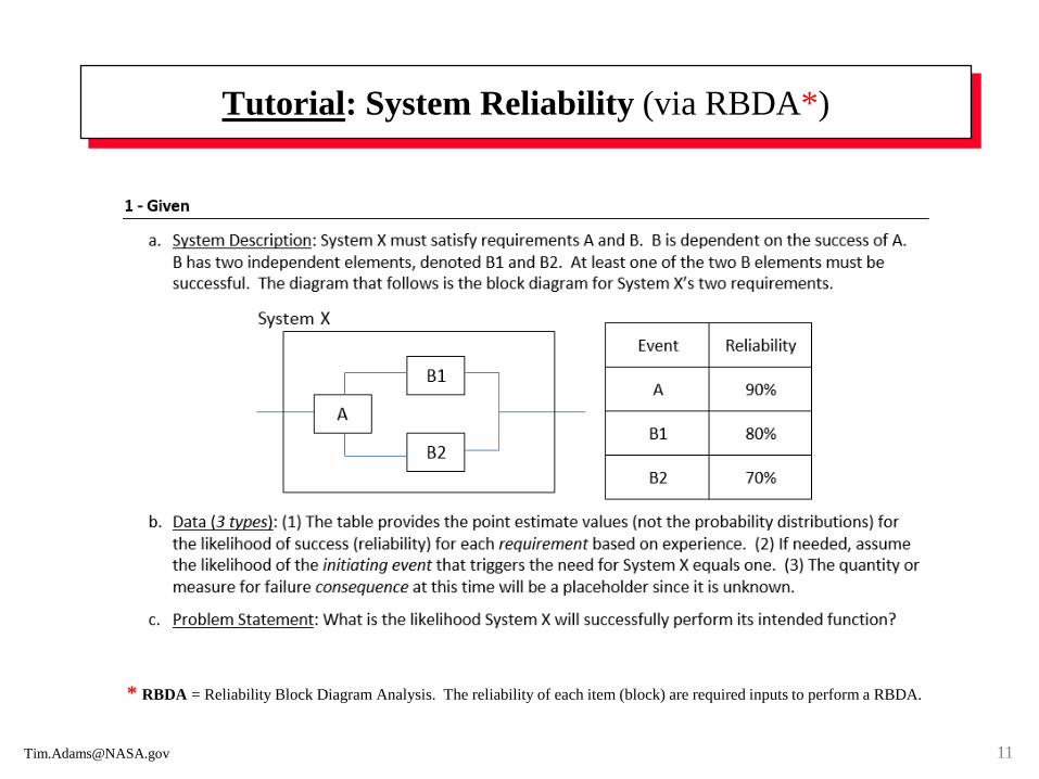
Tutorial: System Reliability (via RBDA*)
11
* RBDA = Reliability Block Diagram Analysis. The reliability of each item (block) are required inputs to perform a RBDA.
Example #1: The Problem
A recent system failure caused major embarrassment as
well as much expense. Should this system be upgraded
or replaced with new technology?
If upgraded, identify the system elements causing the
trouble and the determine the minimum required
reliability to complete missions over the life of the
program.
13

Example #1: This problem occurred with a
Space Shuttle Orbiter’s Fuel Cell
14
A fuel cell on a Space Shuttle Orbiter caused a minimum
duration flight (MDF) during STS-83. In addition to the
MDF, a previous launch delay and numerous
maintenance actions during “vehicle turnaround” made
this subsystem a serious candidate for improvement.
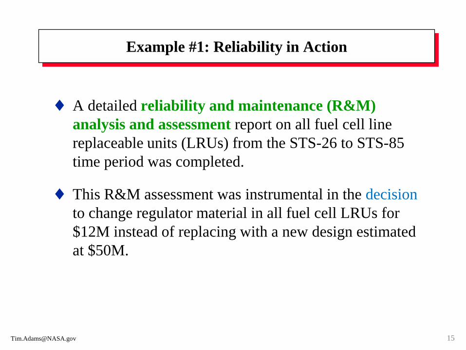
Example #1: Reliability in Action
A detailed reliability and maintenance (R&M)
analysis and assessment report on all fuel cell line
replaceable units (LRUs) from the STS-26 to STS-85
time period was completed.
This R&M assessment was instrumental in the decision
to change regulator material in all fuel cell LRUs for
$12M instead of replacing with a new design estimated
at $50M.
15
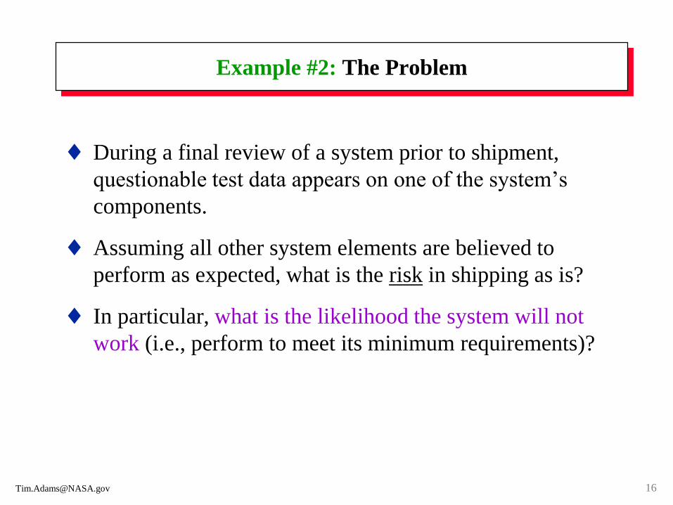
Example #2: The Problem
During a final review of a system prior to shipment,
questionable test data appears on one of the system’s
components.
Assuming all other system elements are believed to
perform as expected, what is the risk in shipping as is?
In particular, what is the likelihood the system will not
work (i.e., perform to meet its minimum requirements)?
16
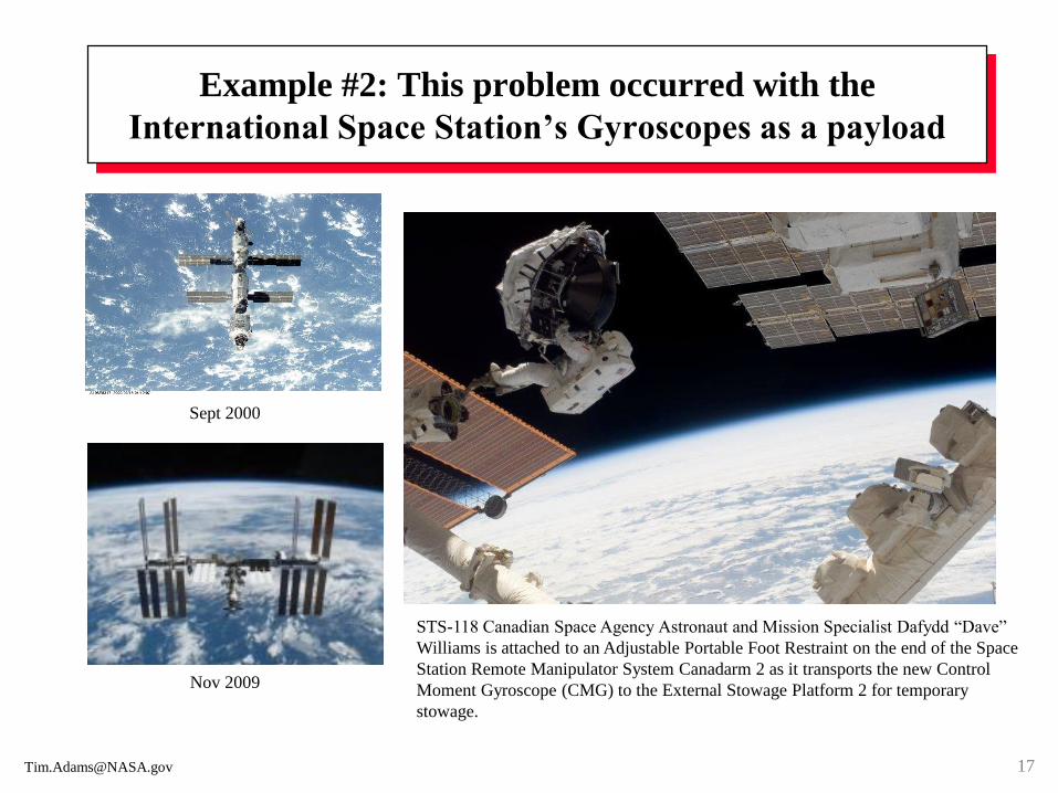
Example #2: This problem occurred with the
International Space Station’s Gyroscopes as a payload
Nov 2009
Sept 2000
STS-118 Canadian Space Agency Astronaut and Mission Specialist Dafydd “Dave”
Williams is attached to an Adjustable Portable Foot Restraint on the end of the Space
Station Remote Manipulator System Canadarm 2 as it transports the new Control
Moment Gyroscope (CMG) to the External Stowage Platform 2 for temporary
stowage.
17
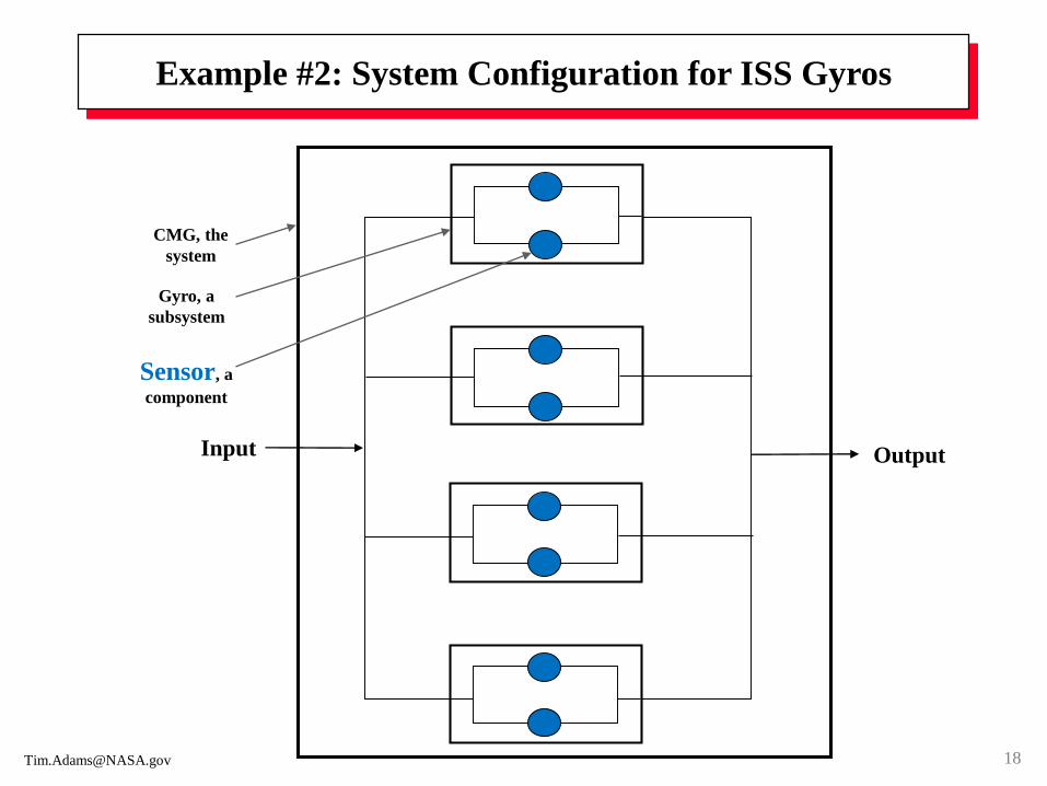
CMG, the
system
Sensor, a
component
Gyro, a
subsystem
Input Output
Example #2: System Configuration for ISS Gyros
18
Example #2: Reliability in Action
Vendor test data generated a concern with the expected reliability of the Hall resolvers (sensors). These sensors are used on the Control Moment Gyros (CMGs), a Space Shuttle payload planned for Space Station’s Flight 3A.
A reliability analysis presented to the Space Station Control Board (SSCB) showed there was a 4-6% chance of not having a minimum CMG. A minimum CMG is at least 1 of 2 sensors working in each gyro and at least 2 of the 4 gyros working for 5, 7, or 9 thermal cycles.
The uncertainty in the thermal-cycle count was because the sensor heaters on the Space Station would not be operational until after the sensors experienced an estimated number of thermal cycles.
The consequence of not having a minimum CMG meant that 6 metric tons of propellant for a reboost would have to be consumed at a cost of $100 million.
The decision was made to ship the CMGs as planned--which proved to satisfy the mission requirements both for the short and long terms.
19
Example #3: The Problem
The test director wants to know: Can testing stop after
receiving no failures in 360 tests on a life-critical item?
In particular, does this testing certify that the item is
safe?
20
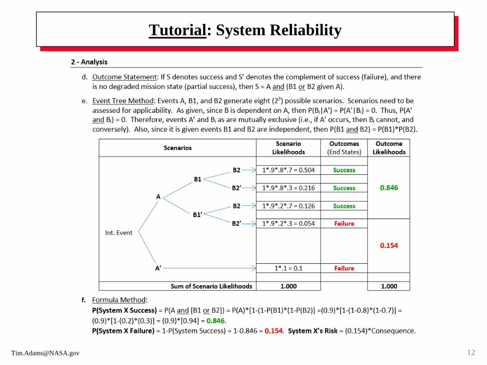
Example #3: This problem pertained to the
Astronaut’s Extravehicular Mobility Unit
21
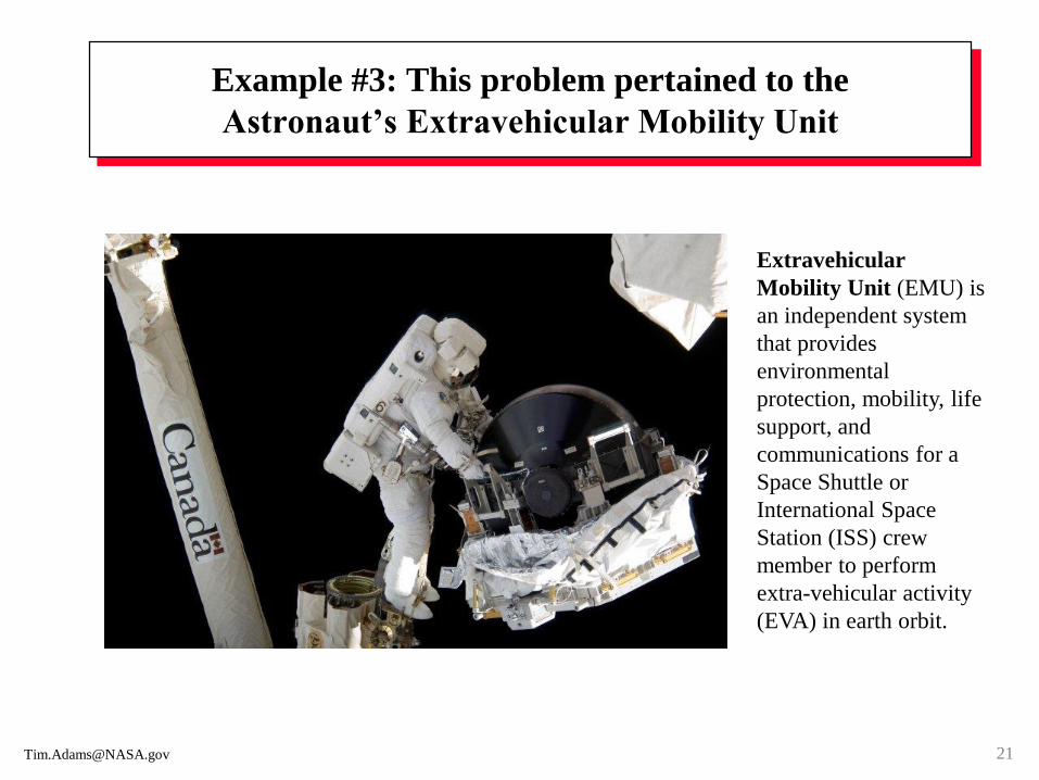
Extravehicular
Mobility Unit (EMU) is
an independent system
that provides
environmental
protection, mobility, life
support, and
communications for a
Space Shuttle or
International Space
Station (ISS) crew
member to perform
extra-vehicular activity
(EVA) in earth orbit.
Example #3: In particular, interpret test data
The White Sands Test Facility (WSTF) conducted 360
tests to determine if ignition would occur during the
presence of a small quantity of hydrocarbon oil in 100%
oxygen under adiabatic compression, the compression
heating of oxygen.
None of the WSTF tests produced ignition. These tests
were in response to a hydrocarbon-oil contaminate
found in the Life Support System (PLSS) used in the
Extravehicular Mobility Unit (EMU).
22
Example #3: Reliability in Action (but limited)
Method 1 used Classical Test Statistics to determine the
maximum failure probability with a high degree of
statistical confidence. This failure probability did not
meet the program’s failure-probability goal. Thus, more
testing required if only this type of analysis (little q) was
used for decision making.
Method 2 used Ancillary Data (i.e., similar test data) to
identify a boundary for ignition and no ignition. This
method was not sufficient for decision making since heat
loss was not addressed.
24
Example #3: Reliability in Action (but limited)
Method 3 used the Arrhenius Reaction Rate Model. This
model (pseudo-big Q) adjusted the failure probability found in
the first method since all WSTF testing was done under
stressed conditions (higher pressure). The failure-probability
goal was surpassed under certain assumptions.
Method 4 used Combustion Physics (Semenov equations) to
address the heat loss not addressed in Method 2. It was found
that the reaction rate was not fast enough to cause ignition in
the PLSS. Thus qualitatively (big Q), the failure-probability
goal was believed (decided) to be satisfied.
25
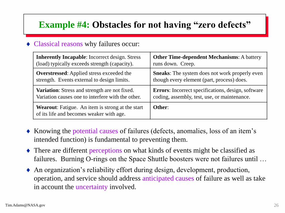
Example #4: Obstacles for not having “zero defects”
Classical reasons why failures occur:
Knowing the potential causes of failures (defects, anomalies, loss of an item’s
intended function) is fundamental to preventing them.
There are different perceptions on what kinds of events might be classified as
failures. Burning O-rings on the Space Shuttle boosters were not failures until …
An organization’s reliability effort during design, development, production,
operation, and service should address anticipated causes of failure as well as take
in account the uncertainty involved.
Inherently Incapable: Incorrect design. Stress
(load) typically exceeds strength (capacity).
Other Time-dependent Mechanisms: A battery
runs down. Creep.
Overstressed: Applied stress exceeded the
strength. Events external to design limits.
Sneaks: The system does not work properly even
though every element (part, process) does.
Variation: Stress and strength are not fixed.
Variation causes one to interfere with the other.
Errors: Incorrect specifications, design, software
coding, assembly, test, use, or maintenance.
Wearout: Fatigue. An item is strong at the start
of its life and becomes weaker with age.
Other:
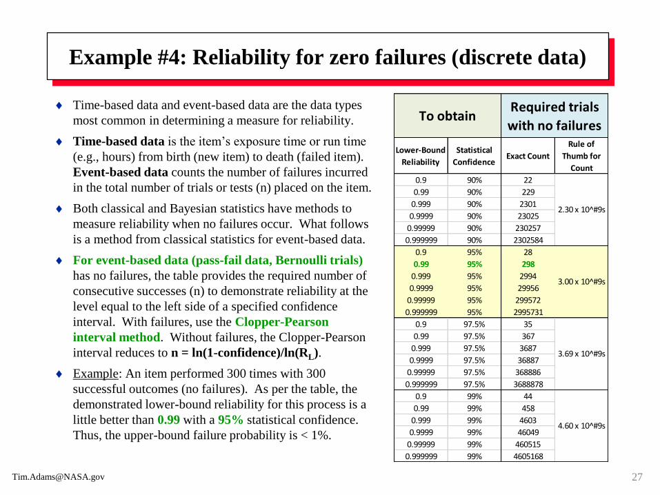
Example #4: Reliability for zero failures (discrete data)
Time-based data and event-based data are the data types
most common in determining a measure for reliability.
Time-based data is the item’s exposure time or run time
(e.g., hours) from birth (new item) to death (failed item).
Event-based data counts the number of failures incurred
in the total number of trials or tests (n) placed on the item.
Both classical and Bayesian statistics have methods to
measure reliability when no failures occur. What follows
is a method from classical statistics for event-based data.
For event-based data (pass-fail data, Bernoulli trials)
has no failures, the table provides the required number of
consecutive successes (n) to demonstrate reliability at the
level equal to the left side of a specified confidence
interval. With failures, use the Clopper-Pearson
interval method. Without failures, the Clopper-Pearson
interval reduces to n = ln(1-confidence)/ln(RL).
Example: An item performed 300 times with 300
successful outcomes (no failures). As per the table, the
demonstrated lower-bound reliability for this process is a
little better than 0.99 with a 95% statistical confidence.
Thus, the upper-bound failure probability is < 1%.
Lower-Bound
Reliability
Statistical
ConfidenceExact Count
Rule of
Thumb for
Count
0.9 90% 22
0.99 90% 229
0.999 90% 2301
0.9999 90% 23025
0.99999 90% 230257
0.999999 90% 2302584
0.9 95% 28
0.99 95% 298
0.999 95% 2994
0.9999 95% 29956
0.99999 95% 299572
0.999999 95% 2995731
0.9 97.5% 35
0.99 97.5% 367
0.999 97.5% 3687
0.9999 97.5% 36887
0.99999 97.5% 368886
0.999999 97.5% 3688878
0.9 99% 44
0.99 99% 458
0.999 99% 4603
0.9999 99% 46049
0.99999 99% 460515
0.999999 99% 4605168
3.00 x 10^#9s
3.69 x 10^#9s
4.60 x 10^#9s
To obtain
2.30 x 10^#9s
Required trials
with no failures
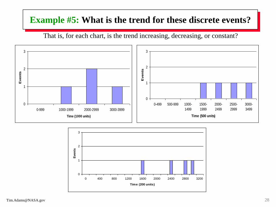
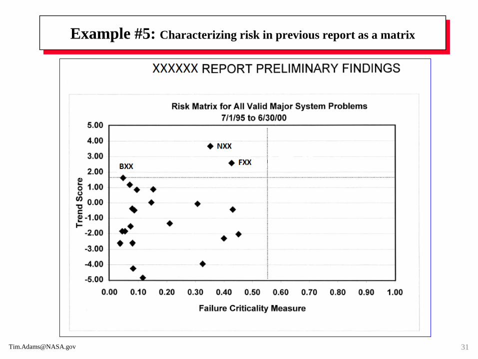
Example #5: What is the trend for these discrete events?
That is, for each chart, is the trend increasing, decreasing, or constant?
0
1
2
3
0-999 1000-1999 2000-2999 3000-3999
Time (1000 units)
Even
ts
0
1
2
3
0-499 500-999 1000-
1499
1500-
1999
2000-
2499
2500-
2999
3000-
3499
Time (500 units)
Even
ts
0
1
2
3
0 400 800 1200 1600 2000 2400 2800 3200
Time (200 units)
Even
ts
28
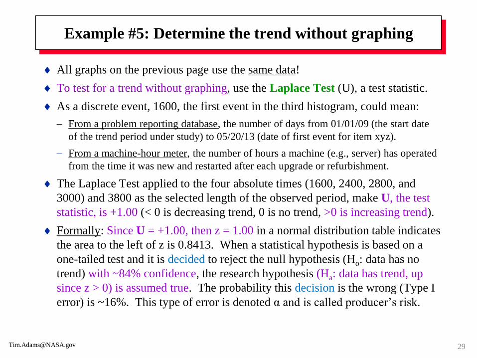
Example #5: Determine the trend without graphing
All graphs on the previous page use the same data!
To test for a trend without graphing, use the Laplace Test (U), a test statistic.
As a discrete event, 1600, the first event in the third histogram, could mean:
From a problem reporting database, the number of days from 01/01/09 (the start date
of the trend period under study) to 05/20/13 (date of first event for item xyz).
From a machine-hour meter, the number of hours a machine (e.g., server) has operated
from the time it was new and restarted after each upgrade or refurbishment.
The Laplace Test applied to the four absolute times (1600, 2400, 2800, and
3000) and 3800 as the selected length of the observed period, make U, the test
statistic, is +1.00 (< 0 is decreasing trend, 0 is no trend, >0 is increasing trend).
Formally: Since U = +1.00, then z = 1.00 in a normal distribution table indicates
the area to the left of z is 0.8413. When a statistical hypothesis is based on a
one-tailed test and it is decided to reject the null hypothesis (Ho: data has no
trend) with ~84% confidence, the research hypothesis (Ha: data has trend, up
since z > 0) is assumed true. The probability this decision is the wrong (Type I
error) is ~16%. This type of error is denoted α and is called producer’s risk.
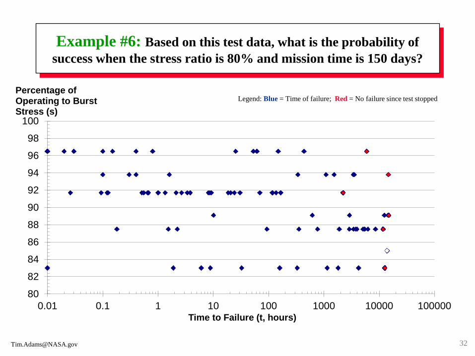
Example #6: Based on this test data, what is the probability of
success when the stress ratio is 80% and mission time is 150 days?
80
82
84
86
88
90
92
94
96
98
100
0.01 0.1 1 10 100 1000 10000 100000
Percentage of Operating to Burst Stress (s)
Time to Failure (t, hours)
Legend: Blue = Time of failure; Red = No failure since test stopped
32
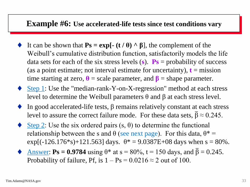
Example #6: Use accelerated-life tests since test conditions vary
It can be shown that Ps = exp[- (t / θ) ^ β], the complement of the
Weibull’s cumulative distribution function, satisfactorily models the life
data sets for each of the six stress levels (s). Ps = probability of success
(as a point estimate; not interval estimate for uncertainty), t = mission
time starting at zero, θ = scale parameter, and β = shape parameter.
Step 1: Use the "median-rank-Y-on-X-regression" method at each stress
level to determine the Weibull parameters θ and β at each stress level.
In good accelerated-life tests, β remains relatively constant at each stress
level to assure the correct failure mode. For these data sets, β ≈ 0.245.
Step 2: Use the six ordered pairs (s, θ) to determine the functional
relationship between the s and θ (see next page). For this data, θ* =
exp[(-126.176*s)+121.563] days. θ* = 9.0387E+08 days when s = 80%.
Answer: Ps = 0.9784 using θ* at s = 80%, t = 150 days, and β = 0.245.
Probability of failure, Pf, is 1 – Ps = 0.0216 ≈ 2 out of 100.
33
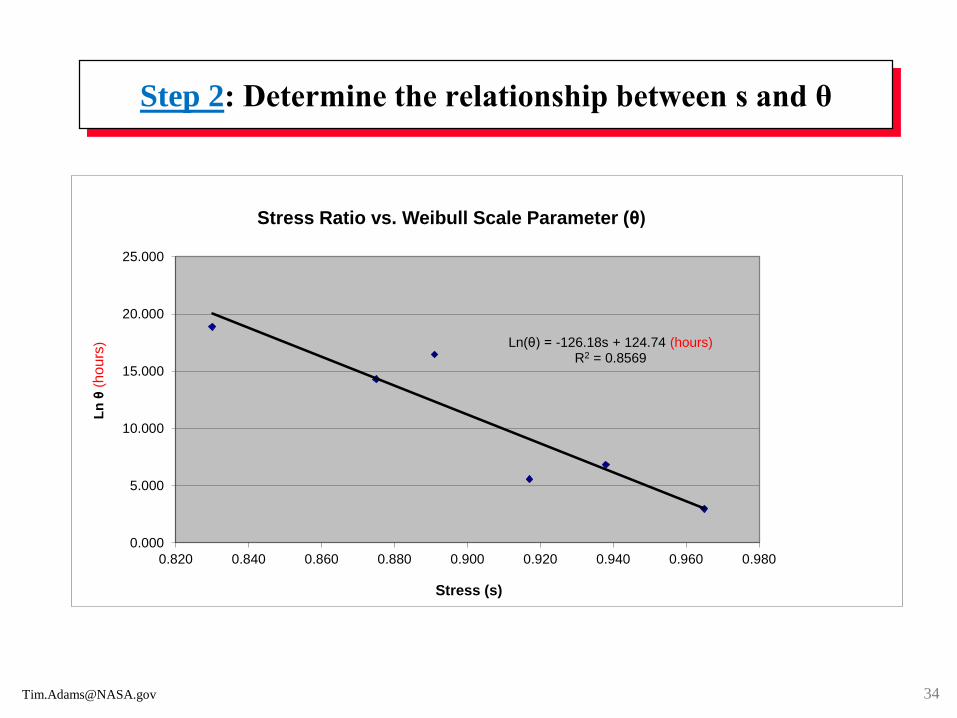
Step 2: Determine the relationship between s and θ
Ln(θ) = -126.18s + 124.74 (hours)R2 = 0.8569
0.000
5.000
10.000
15.000
20.000
25.000
0.820 0.840 0.860 0.880 0.900 0.920 0.940 0.960 0.980
Ln
θ(h
ou
rs)
Stress (s)
Stress Ratio vs. Weibull Scale Parameter (θ)
34
Example #7: Parameter (statistical) uncertainty
Design Objective: Make a survivability metric* with
associated uncertainty for personnel working in the Vehicle
Assembly Building (VAB) to assemble and checkout a
spacecraft. This metric will combine or join two likelihoods
(probabilities), namely,
1. The likelihood of occurrence and
2. The likelihood of impact to personnel
… for various hazards occurring over time, at different
locations, and during different vehicle build phases.
* To provide a metric, the VAB survivability probability for each identified hazard was
compared to the complement or one minus the accident rate for aerospace workers.
Example #7: Analyzing risk in success space
The survivability measure (not metric) for each hazardous scenario,
at each phase, at each zone, and at each time mark was called the
Probability of Survival, P(S), where:
P(S) = 1 - { P(E) * [ 1 - P(S|E) ] }.
P(E), Scenario Likelihood, is the probability of the hazardous scenario
occurring at any or all zones at any phase.
P(S|E), Survival Level, is the probability of survival given the
hazardous event occurred in zone x and phase y. Survival Level ranges
from 0% (death) to 100% (survival).
The formulas for Aggregate Survival Level and Composite Scenarios, a
group of scenarios, are not described here.
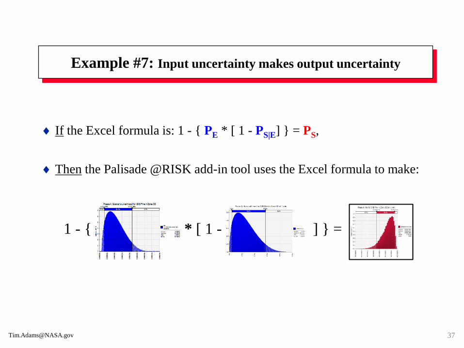
Example #7: Input uncertainty makes output uncertainty
If the Excel formula is: 1 - { PE * [ 1 - PS|E] } = PS,
Then the Palisade @RISK add-in tool uses the Excel formula to make:
1 - { * [ 1 - ] } =
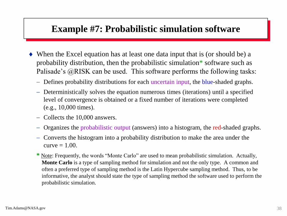
Example #7: Probabilistic simulation software
When the Excel equation has at least one data input that is (or should be) a
probability distribution, then the probabilistic simulation* software such as
Palisade’s @RISK can be used. This software performs the following tasks:
Defines probability distributions for each uncertain input, the blue-shaded graphs.
Deterministically solves the equation numerous times (iterations) until a specified
level of convergence is obtained or a fixed number of iterations were completed
(e.g., 10,000 times).
Collects the 10,000 answers.
Organizes the probabilistic output (answers) into a histogram, the red-shaded graphs.
Converts the histogram into a probability distribution to make the area under the
curve = 1.00.
* Note: Frequently, the words “Monte Carlo” are used to mean probabilistic simulation. Actually,
Monte Carlo is a type of sampling method for simulation and not the only type. A common and
often a preferred type of sampling method is the Latin Hypercube sampling method. Thus, to be
informative, the analyst should state the type of sampling method the software used to perform the
probabilistic simulation.
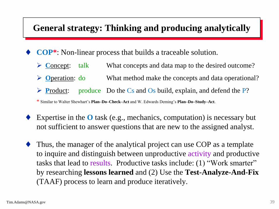
General strategy: Thinking and producing analytically
COP*: Non-linear process that builds a traceable solution.
Concept: talk What concepts and data map to the desired outcome?
Operation: do What method make the concepts and data operational?
Product: produce Do the Cs and Os build, explain, and defend the P?
* Similar to Walter Shewhart’s Plan–Do–Check–Act and W. Edwards Deming’s Plan–Do–Study–Act.
Expertise in the O task (e.g., mechanics, computation) is necessary but
not sufficient to answer questions that are new to the assigned analyst.
Thus, the manager of the analytical project can use COP as a template
to inquire and distinguish between unproductive activity and productive
tasks that lead to results. Productive tasks include: (1) “Work smarter”
by researching lessons learned and (2) Use the Test-Analyze-And-Fix
(TAAF) process to learn and produce iteratively.
39

Practice COP with the customer before the “due date”
With analytical-type work, there are advantages when the analyst is
able to communicate with the decision maker while the analytical
work is in the design (conceptual) and build (operational) phases.
“…only 40% of projects suggested by quantitative analysts were
ever implemented. But 70% of the quantitative projects initiated by
users, and fully 98% of projects suggested by top managers, were
implemented.”Barry Render & Ralph M. Stair Jr., Quantitative Analysis for Management, 6th edition
And because … see next page.
40
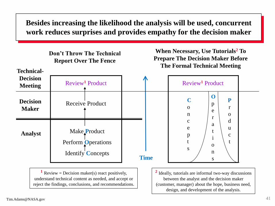
Besides increasing the likelihood the analysis will be used, concurrent
work reduces surprises and provides empathy for the decision maker
Time
Don’t Throw The Technical
Report Over The Fence
When Necessary, Use Tutorials2 To
Prepare The Decision Maker Before
The Formal Technical Meeting
Decision
Maker
Analyst Make Product
Perform Operations
Identify Concepts
C
o
n
c
e
p
t
s
P
r
o
d
u
c
t
O
p
e
r
a
t
i
o
n
s
Receive Product
2 Ideally, tutorials are informal two-way discussions
between the analyst and the decision maker
(customer, manager) about the hope, business need,
design, and development of the analysis.
Technical-
Decision
Meeting Review1 Product Review1 Product
41
1 Review = Decision maker(s) react positively,
understand technical content as needed, and accept or
reject the findings, conclusions, and recommendations.
Analyst Mantras
“Success comes in cans, not in cannots!”Joel H. Weldon, motivational speaker
“Think about your thinking.” The 7 Levels of Change, Rolf Smith
“Do you think if you torture the data long enough it will confess to
you?” Dr. Harold V. Huenke, Professor of Mathematics, University of Oklahoma.
Update: Mark Hulbert’s Sept 26, 2006 Market Watch stated, “If you torture the data long enough, you can get it to say just
about anything.”
“Somebody is going to have to suffer, either the reader or the writer.”Tom Murawski, national leader in writing improvement, The Murawski Group Inc
“A perfect world is when ‘big Q’ (qualitative view) and ‘little q’
(quantitative view) agree--or at least understand why not to agree!”Author
42