Embed Size (px)
Citation preview

HU ISSN 1785-6892 (PRINT)
HU ISSN 2064-7522 (ONLINE)
DESIGN OF MACHINES AND STRUCTURES
A Publication of the University of Miskolc
Volume 4, Number 2 (2014)
Miskolc University Press
2014


HU ISSN 1785-6892 (PRINT)
HU ISSN 2064-7522 (ONLINE)
DESIGN OF MACHINES AND STRUCTURES
A Publication of the University of Miskolc
Volume 4, Number 2 (2014)
Miskolc University Press
2014

EDITORIAL BOARD
Á. DÖBRÖCZÖNI Department of Machine- and Product Design
Editor in Chief University of Miskolc
H-3515 Miskolc-Egyetemváros, Hungary
Á. TAKÁCS Department of Machine- and Product Design
Assistant Editor University of Miskolc
H-3515 Miskolc-Egyetemváros, Hungary
R. CERMAK Department of Machine Design
University of West Bohemia
Univerzitní 8, 30614 Plzen Czech Republic
B. M. SHCHOKIN Consultant at Magna International Toronto
W. EICHLSEDER Institut für Allgemeinen Maschinenbau
Montanuniversität Leoben,
Franz-Josef Str. 18, 8700 Leoben, Österreich
S. VAJNA Institut für Maschinenkonstruktion,
Otto-von-Guericke-Universität Magdeburg,
Universität Platz 2, 39106 MAGDEBURG, Deutschland
P. HORÁK Department of Machine and Product Design
Budapest University of Technology and Economics
H-1111 Budapest, Műegyetem rkp. 9.
MG. ép. I. em. 5.
K. JÁRMAI Department of Materials Handling and Logistics
University of Miskolc
H-3515 Miskolc-Egyetemváros, Hungary
L. KAMONDI Department of Machine- and Product Design
University of Miskolc
H-3515 Miskolc-Egyetemváros, Hungary
GY. PATKÓ Department of Machine Tools
University of Miskolc
H-3515 Miskolc-Egyetemváros, Hungary
J. PÉTER Department of Machine- and Product Design
University of Miskolc
H-3515 Miskolc-Egyetemváros, Hungary

CONTENTS
Dömötör, Csaba: Statistical analysis of natural analogy catalogue ....................................... 5
Kiss, Dániel–Csáki, Tibor: Reverse engineering at the University of Miskolc.................... 13
Lyssenko, Valery–Konogonov, Serguey–Zolotarevskiy, Serguey: Different methods for
a 3D measurements of surface roughness etalons ................................................................ 19
Poroshin, Valery–Bogomolov, Dmitry–Poroshin, Oleg–Lyssenko, Valery:
High precision automated measurement system for 3D analysis of surface texture
at the nanoscale .................................................................................................................... 27
Poroshin, Valery–Bogomolov, Dmitry–Anosova, Anna–Radygin Victor: Mesoscopic
lattice-Boltzmann modelling of flow in thin channel with rough walls ............................... 35
Sheipak, Anatoly–Novikov, Pavel: The satellite-based algorithm for determining
the location of hydraulic lift ................................................................................................. 45
Takács, Ágnes: Generating concepts with the help of green tips ......................................... 53
Tóth, Dániel: Examination of ball bearing using stochastic indexes ................................... 59
Tóth, Dániel–Szilágyi, Attila–Takács, György: Vibration analysis techniques for
rolling element bearing fault detection ................................................................................. 65


Design of Machines and Structures, Vol 4, No. 2 (2014) pp. 5–12.
STATISTICAL ANALYSIS OF NATURAL ANALOGY CATALOGUE
CSABA DÖMÖTÖR
University of Miskolc, Department of Machine and Product Design
3515, Miskolc-Egyetemváros
Abstract: In the methodical machine designing the analogy based design methods are very important
ways to reach the optimal solution of a particular problem. In such cases intuition is significant tool
for engineers, which needs preexistent acquirements and experiences. Man knows for a long time past
that the largest experience-collection is accumulated in the nature. This article will show how we can
transform it to technical practice.
Keywords: natural structures, bionics, biomimetics, design principles, natural adaptation, statistical
analysis
1. Introduction
In natural sciences there is a view, which has recently gained widespread acceptance,
according to which finding the optimal solutions for technical problems in effect principles
and effect carriers of the living and lifeless environment can be an efficiently adaptable
option not only in research and development, but also in general engineering practice. This
relatively new way of thinking has been justified by several products used in everyday life
which show significant similarities with solutions in the living world.
For the rise of the application of natural analogies out of specialized fields it is
inevitable for us to categorize, classify and teach them from an engineering aspect. The
main findings of this paper reflect this effort, together with a database corresponding with
an engineering approach and algorithms supporting its application which based on the well-
known general problem solving model (Figure 1).
Figure 1. General problem solving model [1]
2. Directions of bionics
In the literatures of the science findings in bionics as well as biomimetics we
differentiate between analogue and abstract procedures of natural adaptations [2]. In other
sources analogue direction is called as “top-down” or “technology pull” procedure because
analogue way starts from a particular technical problem and tries to find a special adaptable
solution from nature (Figure 2) [10].
Particular solution
Analogous
solution
Analogous problem
Particular problem

6
Csaba Dömötör
Example:
Improve sport-achievements
– Minimize resistance of continuum
– Develop proper movements
Analysis of
– surfaces,
– shapes and
– movements of fast animals and objects
– Flexible objects take on the shape of raindrop
– Sharks reduce convection loss through special
ridgy shape of fish-scales
– Streamlined drop-shape helmet
– Special plating swimsuit
Figure 2. Main processes of analogue procedure [3]
In the steps of analogue procedure (Figure 2) it is easy to recognize the main stations of
analogy based problem solving model (Figure 1) which useable for engineers long ago.
Abstract direction is a reverse process. At the same way to previously the alternative
names of this are “bottom-up” or “biology push” procedure because in this case the starting
base is a special biological effect and constructors try to find the potential employments of
this and so create a new product. To reach this goal the abstraction gives the most important
step of this process (Figure 3).
Example:
Nails of thistles cling to fur of animals.
Plants insure expansion of their population through
climbing of ripe seeds to walking animals.
Abstraction:
Temporary fixing function
Useful for quick and simple fastening and unfastening
in various fields
Velcro – hooks and loops replace with nylon fibres
Figure 3. Main processes of abstractive procedure [3]
Detect a special
biological effect
Compose
natural challenge
Search potential
employment
Develop new
product
Define
problem
Search analogies
in nature
Analysis of
organic solutions
Develop
own solution

Statistical analysis of natural analogy catalogue
7
Essence of abstraction is that man able to explain occurrence over observation and in
this way able to apply this experience in another field of science. How block diagram of
analogue procedure shows similarity with general problem solving model likewise it is
suggestive to sketch generalized model of abstraction (Figure 4) from the flow chart of
abstractive procedure of natural adaptation (Figure 3) because it shows perfectly the
different way of thinking which is based on diverse start-points.
Figure 4. Generalized model of abstraction
The main steps of generalized model of abstraction are able to summarize with 3 short
question-words:
Step 1: Why?
Why must take it such as it is? In most cases it is recognizable the original problem
or previous challenge which gives good base for abstraction.
Step 2: Where?
Where could man use it? It is necessary to define a similar technical problem and
recognize one or more realizable innovative employments.
Step 3: How?
How could man realize it in a new product? The main mission is to develop a
producible and saleable product with the mindful of technology possibilities and
market conditions.
Relying on the natural analogy database this resource work is established that natural
analogies account for 69% of the solutions in the analogue direction while the adaptations
in an abstractive way account for 31%.
3. Catalogue of natural analogies
The main part of the research which shown in this paper is the classification of natural
analogies according to engineering subfields as well as the presentation of their expressive
examples, in which the two main groups are shapeforming elements and constructive
solutions. As this paper cannot present analogies, data types and surfaces of the database
are uploaded and shown in detail in Microsoft Access format and are available as electronic
appendices. The computer-based analogy catalogue made it possible to categorize and
analyze the detected similarities according to content, direction and – within it – awareness.
On the basis of this taxonomy it is studied the complex data quantity of natural analogies
from a new point of view and analyzed their positions in the design process.

8
Csaba Dömötör
3.1. Awareness as subcategory of two directions
Considering the records of the catalogue as being representative, it is realized that about
73% of natural analogies cannot be classified as the results of conscious search for an
analogy. A part of these analogies is based on a posterior recognition, another part is the
result of spontaneous matching of images in the designer’s subconscious (Figure 5).
Figure 5. Directions of bionics and its subcategories [4]
3.2. Technical content levels
In analogy catalogue the classification of natural analogies according to technical
content differentiate between three categories. These equally dispersed levels of Theory,
Form and Function are realized in a hierarchy (Figure 6).
The depth of similarity can realize in 3 levels:
Level 1: Analogy in Theory
– The principle effect is the same between natural and technical solution, but the main
function does not -or not unconditionally- show similarity.
(e.g.: eye-spots dummy security cameras)
Level 2: Analogy in Form
– There are recognizable essential geometrical similarities in effect carriers which
realize the same principle in case of the technical and the organic example but from
the point of view of final employing the performed function is not exactly the same.
(e.g.: gecko nanopad)
Level 3: Analogy in Function
– The two parts of natural analogy-pairs realize the same function and there are
recognizable similarities in shape which attains the same basic principle.
(e.g.: ears of the African elephant cooler of cars)
It is born a new technical solution from a
nature principle with conscious search.
The evident solution of a technical
problem coincide with a nature principle.
It starts from a technical problem and
search solution consciously in nature.
A technical problem was solved with
traditional method but afterwards a
similar solution is recognizable in nature.
Applied
Spontaneous
Analogue
TECHBIOS
Abstractive
BIOSTECH
Natural
analogies
Explored
Posterior

Statistical analysis of natural analogy catalogue
9
Figure 6. Hierarchy of technical content of natural analogies
On the basis of analysis of the records of natural analogy catalogue it is ascertainable
that a natural adaptation is formal analogy only then the realized principle is also the same
in technical and natural side. The functional analogies give the highest level of similarities
where not only the principle effect and effect carriers are the same but realized final aim is
harmonious too.
4. Algorithm
It is most important to integrate the similarities with nature into an existing analogy-
based method. For this goal this paper presents the algorithms of processes called
Abstractive adaptation and Improvement with well-known analogies on the basis of
biological discoveries carrying special basic principles.
4.1. Algorithm for abstractive procedure
Starting from the generalized model of abstraction (Figure 4) it is worked out the
algorithm of abstractive procedure of biomimetics that is showed in Figure 7.
4.2. Algorithm of improvement for analogue procedure
It is worked out the algorithm of improvement with well-known natural analogies
(Figure 8). In this way it has proven that after the definition of environmental conditions
and biological opportunities the Posterior analogies accounting for 66% of the database are
suitable to improve and develop engineering pieces of work in a special way.
Level 3
same function
Level 2
similar form elements
Level 1
same principle

10
Csaba Dömötör
Figure 7. Algorithm for abstractive procedure

Statistical analysis of natural analogy catalogue
11
Figure 8. Algorithm of improvement for analogue procedure

12
Csaba Dömötör
5. Conclusions
On the basis of the findings it can clearly define the deficiencies that are the main
obstacles of the application of the numerous solutions in nature. The described procedure is
able to combine with the catalogue which possibility gives the theoretical basis for the
computer-aided search for natural analogies and this way the application of natural
principles in general engineering practice can become the permanent part of conceptual
design process [11].
6. Acknowledgements
The research work presented in this paper based on the results achieved within the
TÁMOP-4.2.1.B-10/2/KONV-2010-0001 project and carried out as part of the TÁMOP-
4.1.1.C-12/1/KONV-2012-0002 “Cooperation between higher education, research institutes
and automotive industry” project in the framework of the New Széchenyi Plan. The
realization of this project is supported by the Hungarian Government, by the European
Union, and co-financed by the European Social Fund.
7. References
[1] Mazur, G. H.: Theory of Inventive Problem Solving (TRIZ). University of Michigan College of
Engineering, 1995.
[2] VDI 6220: 2011-06 Bionik; Konzeption und Strategie; Abgrenzung zwischen bionischen und
konventionellen Verfahren/Produkten (Biomemetics; Conception and strategy; Differences
between bionic and conventional methods/products). Beuth Verlag, Berlin.
[3] Dömötör, Cs.: Natural motivations in engineering design. Gép, 2005 (56. évf.) 9-10. sz. pp. 5–26.
[4] Dömötör, Cs.: A természeti intuíció hatása a termékfejlesztés gyakorlatára. Gép, 2014, Vol. 65,
No. 2, pp. 23–26.
[5] Benyus, J. M.: Biomimicry: innovation inspired by nature. Harper Perennial, 2002.
[6] Péter, J.–Dömötör, Cs.: Principles of the design theory and the nature. XXVI. MicroCAD
International Scientific Conference, Miskolc, March 29–30, 2012.
[7] Péter, J.– Dömötör, Cs.: Industrial design in development. Miskolc-Egyetemváros, 2011.
[8] Pahl, G.–Beitz, W.: Konstruktionslehre – Handbuch für Studium und Praxis. Springer-Verlag,
Berlin, 1981.
[9] Roth, K.: Konstruiren mit Konstruktionskatalogen. VEB Verlag Technik, Berlin, 1982.
[10] Nachtigall, W.: Bionik: Grundlagen und Beispiele für Ingenieure und Naturwissenschaftler.
Springer, Berlin–Heidelberg, 2002.
[11] Takács Á.: Termékek számítógéppel segített koncepcionális tervezési módszereinek kutatása.
PhD-értekezés, Miskolc-Egyetemváros, 2009.
[12] Hansen, F.: Konstruktionssystematik – Grundlagen für eine allgemeine Konstruktionslehre. VEB
Verlag Technik, Berlin, 1965.
[13] Koller, R.: Konstruktionslehre für den Maschienenbau. Springer-Verlag, Berlin, 1985.

Design of Machines and Structures, Vol 4, No. 2 (2014) pp. 13–18.
REVERSE ENGINEERING AT THE UNIVERSITY OF MISKOLC
DÁNIEL KISS–TIBOR CSÁKI
University of Miskolc, Institute of Machine Tools and Mechatronics
3515, Miskolc-Egyetemváros
Abstract: An industrial project will be presented in this paper about reverse engineering. We have to
reproduce the blades of a mixing turbine without drawing. After 3D scanning and model creating we
generated toolpath using CAM software to produce the component, and manufacture the workpiece.
Keywords. 3D scanner, free form surface, reverse engineering
1. The problem
After long hours of run in harsh environment components may suffer from different
defects such as distortion, impact dents and wear. Components with freeform surfaces are
nearly impossible to reproduce without the original documentation. If we can scan the part
using a 3D scanner, we can get an 3D model which can be modified in order to get the
desired and repaired shape of the problematic component.
In this case the problematic component was the blades of a mixing turbine which is used
in acidic environment. The original blades was worn out, and have to be replaced, but there
was no data about the shape of the blades except the complete turbine itself. After we
obtain a surface model we can use it as an input for a CAM software to generate the
toolpath for freeform surfaces [1], [3].
Figure 1. The damaged turbine blades

14 Dániel Kiss–Tibor Csáki
Data acquisition
hardware (optical
scanner)
3D scan data
(STL)
Reverse engineering
Correct scanning
errorsRepair worn part
Create CAD
model
Define toolpath
Import CAD
model into CAM
environment
Create NC
programme
Mill the part
Figure 2. Flowchart of the revesre engineering process
2. Hardware and software
In the following sections we present the software and hardware that we used during the
reverse engineering process.
2.1. 3D scanner and related software
The scanning device which is used for the procedure was a Breuckmann Smart Scan
3D-HE mobile optical scanner with Optocat 2009 data acquisition software, which
provided us an STL file [2].
Figure 2. The optical scanner

Reverse engineering at the University of Miskolc
15
The scanned surface can contain defects like spikes and holes. To correct these we used
Geomagic Studio, where we can use different options to repair different defects to get a
smooth surface [1].
Figure 3. Trimming the welding in Geomagic Studio
After the model repair we cut off the welding joint from the surfaces and created a
closed body by filling the hole. Eventually we created a CAD file in STEP format,
containing NURBS surfaces, which is slightly modified in NX to align the inner and outer
radius of the blade. Finally we had a CAD model which was adequate for the CAM
software.
2.2. CAM software
Figure 4. Position of the workpiece on the machine table in CAM software

16 Dániel Kiss–Tibor Csáki
We have used Topsolid 2012 which is an integrated CAD-CAM software suite.
Additional supports had to be drawn for the fixture on the table of the milling machine.
Because of the small workspace of our machine we had to divide the entire model into four
segments. The machining processes in each segment consisted of a 2,5D roughing and
semi-finishing followed by a 3D finishing process. After the milling process is defined, we
created an NC file, using the post processor which is fitted to our milling machine [4].
The milling machine was a DMG DMU40 monoblock 5 axis milling machine with a
workspace of 400x400x450 mm. The tools was a Walter F4041 shoulder milling cutter and
Korloy FMRS 2000 toroidal milling cutter.
Figure 5. Machining of the blade
When the machining process was finished the mounting supports had to be machined
off from the blade. These supports were removed manually. At the the end four blades were
welded on the turbine hub.
Figure 6. The finished turbine

Reverse engineering at the University of Miskolc
17
3. Comparison of the model and the machined part
After the first part was machined, made of plastic (PA6), it was scanned again and
compared with the CAD model. This comparison was made with the Geomagic Studio
Software. The scanned model was corrected from scanning errors then aligned with the
original model. The standard deviation from the CAD model was around 0,233 mm [2].
Figure 7. Comparison of first side
Figure 8. Comparison of second side
4. Summary
During completing the project it revealed that the available tools and hardware together
with the needful software are suitable for reverse engineering application and able to
produce the required quality.

18 Dániel Kiss–Tibor Csáki
5. Acknowledgement
“This research was carried out as part of the TÁMOP-4.2.1.B-10/2/KONV-2010-0001
project with support by the European Union, co-financed by the European Social Fund, in
the framework of the Centre of Excellence of Mechatronics and Logistics at the University
of Miskolc.”
6. References
[1] Gao, Jian–Chen, Xin–Zheng, Detao–Yilmaz, Oguzhan–Gindy, Nabil: Adaptive restoration of
complex geometry parts through reverse engineering application. Advances in Engineering
Software, 37 (2006), pp. 592–600.
[2] Szilágyi, Attila–Csáki, Tibor–Makó, Ildikó: An up-to-date method of dimension control of
freeform surfaces. microCAD 2012, L section: XXVI. International Scientific Conference,
ISBN:978-963-661-773-8
[3] Bandera, C.–Filippi, S.–Moty, B.: CISM International Centre for Mechanical Sciences Reverse
Engineering of a Turbine Blade: Comparison Between two Different Acquisition Techniques.
Advanced Manufacturing Systems and Technology, Volume 486, 2005, pp. 635–644
[4] She, Chen-Hua–Chang, Chun-Chi: Study of applying reverse engineering to turbine blade
manufacture. Journal of Mechanical Science and Technology, October 2007, Volume 21, Issue
10, pp. 1580–1584.

Design of Machines and Structures, Vol 4, No. 2 (2014) pp. 19–25.
DIFFERENT METHODS FOR A 3D MEASUREMENTS OF SURFACE
ROUGHNESS ETALONS
VALERY LYSSENKO–SERGUEY KONONOGOV–SERGUEY ZOLOTAREVSKIY
Russian Research Institute for Metrological Service
115280, Avtozavodskayast. 16, Moscow, Russia
Abstract: Scanning probe microscopes (SPM) are a family of instruments used for studying surface
topography. But it is difficult to select object for testing SPMs. So the investigation of metrological
characteristics of the atomic-force microscope (AFM) “NanoScan” (Russia), AFM “Nanotop”
(Belarus) SPM P4-SPM-MDT (Russia) devices Talystep and Nanostep, Interference-microscope was
worked out.
Keywords: scanning probe microscope, interference microscope, contact stylus profilometer,
nanometrology
1. Introduction
Under term – “nanotechnology” we understand creating and using of materials, devices
and systems, structure which contain in nanometer range. Nanometrology is science and
practice for metrological assurance quality of nanotechnology. For measuring objects of
nanotechnology a lot of measuring equipment of geometrical values are applied. All of
them are 2Dimensional and 3Dimensional coordinate – measuring devices of nanometer
range. Among them accuracy of measurement geometrical values till present time not
enough assured. For metrological assurance of nanotechnology are very important the next
tasks:
To investigate the accuracy ability of the 2D and 3D measuring devices worked in
nanometer range;
To define how to execute calibration and verification of coordinate measuring devices
with nanometer range of working;
Scanning probe microscope (SPM) are a family of instruments used for studying surface
topography and properties of materials at the atomic to micron level. Their metrological
support is non-satisfactory, because it is difficult to select object for testing SPM and
compare the results of measurements of this object by different methods.
As a rule for coordinate measuring machines it is necessary to execute calibration of
working volume in the X0Y plane (for measuring in X0Y plane) and along Z axis (for
measuring of height along Z axis). In plane X0Y this calibration usually executes with help
diffraction grid.
In this work for calibration in X0Y plane we used two diffraction grid: the first –
produced by “LOMO” company (Russia), – the second – produced by “Holograit”
company, calibrated in BIPM (France).
As the standard of height it may be used separate block gauges or unite standard,
consisted from three or more heights.
We used for calibration of measuring devices along Z axis the set of 3D nanostructures
consisted from different configurations of height with nominal 7 nm, 70 nm, and 800 nm.
This set of standards was complimentary given to us by our colleges from PTB (Germany).

20 Valery Lyssenko–Serguey Kononogov–Serguey Zolotarevskiy
We studied the metrological characteristics of the atomic-force microscope (AFM)
planar technology with known geometrical sizes. These test-objects were obtained in our
disposal from PTB, Braunshweig, Germany.
We compare our results with analogous measurements by other devices such as AFM
“Nanotop” from Metal-Polymer Systems Institute of Byelorussian Academy of Science,
Scanning Probe Microscope P4-SPM-MDT from Nanotechnology MDT Inc., Russia,
devices Talystep and Nanostep, Interference-microscope and others.
We propose to discuss the problems of creation the standard metrological security of the
devices for surface parameters measurements with nanometer scale resolution.
2. Method of scanning probe microscopy
In AFM [1] the tip with radius of curvature commensurable with the atomic size in
located near to a surface in a scope of atomic forces. Thus the area of contact between tip
and surface can be about the sizes of atom. Force between probe tip and a surface is used as
probing interaction in AFM. Probe tip can positioning as in the range of repulsion forces
and in the range of Van der Vaals attractive forces when AFM functioning, accordingly
contact and noncontact mode. The probe on which tip is fixed reacts to value of these
forces. On its reactions determine mechanical properties of a surface of researched object
and its geometry. In the majority modern AFM a bend of a console beam with a tip fixed on
its end supervises by optical methods. Microscopes in which cantilever with a tip is
oscillating and tip to an investigation surface contact change of frequency or amplitude are
known.
All SPM are devices of a scanning type. During scanning observation of a surface
adequate a constant level force active between a probe and surface or tunnel current is
carried out. Devices based on the above-stated principles allow to receive the images of
surfaces with the horizontal and vertical resolution up to 0,1 nm that is their basic
advantage before optical. On this parameter they do not concede scanning electronic
microscopes (SEM). Besides these devices allow to measure height relief in a large range
and with the height resolution, that is inaccessible SEM. The simplicity of use SPM, their
universality and more simple interpretation received data gives them significant advantages
before SEM not only in scientific researches but also in technological applications.
In submitted work the described above objects were investigated on AFM NanoScan,
developed and production by HTE Co., Moscow, Russia. This device works in a so-called
contact dynamic mode of scanning. The principles of this mode consists that tip contact
with a surface is fixed on the end of the oscillation console. This mode of work is sensitive
to the mechanical characteristics of a surface material that enables to receive relief both
viscous surfaces and rigid being under a viscous layer. The last peculiarity is especially
important for research of objects on air, when on surface is present absorption a viscous
layer, which smooth down relief elements. Besides, the device allows mapping a surface
mechanical properties (Young modulus) and to measure hardness by an indentation and
sclerometry methods with submicroand nanometer scale. The results received at
measurement on NanoScan topology of a test-objects surface were compared to data,
received at research of the same objects on following AFM.
AFM NanoScan, developed and production by HTE Co., Moscow, Russia used the
noncontact mode of scanning (bend cantilever under influence of attractive forces is
supervised – Figure 1).

Different Methods for a 3D measurements of surface roughness etalons 21
Figure 1. AFM NanoScan
P4-SPM-MDT from Nanotechnology MDT Inc., Moscow, Russia used the contact
mode of scanning (bend cantilever under influence of repulsion forces is supervised –
Figure 2).
Figure 2. P4-SPM-MDT
In particular, the comparison was carried out by results of received on the following
samples, which represent structures from SiO2 on a silicon substrate (Figure 3): Strip of
height 7 nm; Strip of height 70 nm; Square grid with a step 4 microns and depth about 0.5
microns.

22 Valery Lyssenko–Serguey Kononogov–Serguey Zolotarevskiy
a) Strip of height 7 nm
b) Strip of height 70 nm
c) Strip of height 800 nm
Figure 3. Gauges
Received results have allowed to make the following conclusions. The test object as a
square grid can be used for determination of the scanning field sizes and coordinates system
nonlinearity in a XY plane. As a whole, the spent researches have confirmed perspective of
similar test-objects application for calibration of various SPM parameters.
Table 1
Results of measurements
Devices
Test-objects
Square grid Strip 7 nm Strip 70 nm
step, m depth, m Measured height, nm Measured height, nm
NanoScan 4 0.1 0.5 0.1 7 1 70 5
NanoTop 4 0.1 0.4 0.1 – –
P4-SPM-MDT 4 0.5 0.5 0.2 8 1 70 10
Comparisons of measuring ability different scanning probe microscopes
3. Method of interference microscopy
The next device the new modification of interference microscope MII-4 was developed
for the automatic identification of the achromatic land in white light interferometers and for
the digital measurements of its centre position.

Different Methods for a 3D measurements of surface roughness etalons 23
But new modification New View 6200 (Figure 5) is a powerful tool for characterizing
and quantifying surface roughness step heights critical dimensions and other topographical
features with excellent precision and accuracy.
Figure 4. Interference microscope MII-4
The new modification of interference microscope MII-4 (Figure 4) was developed for
the automatic identification of the achromatic land in white light interferometers and for the
digital measurements of its centre position. It can:
– to automatic the measuring process in white light;
– to control processing of data with a computer;
– to display (or print) graphics and digital information about object under
investigation;
– to increase the accuracy and sensitivity of interferometric methods and widen in
the range of measurement both of low and high film thickness.
Figure 5. Zygo New View 6200
So, with these interferometers we can measure profiles of the surfaces with high
accuracy.
In interference microscope MII-4 the wavelength is used as standard (it is the natural
standard). Therefore this interferometer can be used as primary standard for traceability in
nanometer range. The New View 6200 can be used as reference standard for traceability of
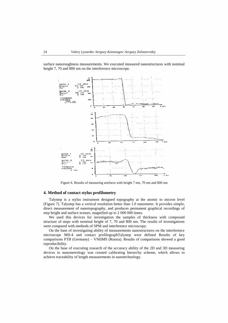
24 Valery Lyssenko–Serguey Kononogov–Serguey Zolotarevskiy
surface nanoroughness measurements. We executed measured nanostructures with nominal
height 7, 70 and 800 nm on the interference microscope.
Figure 6. Results of measuring artefacts with height 7 nm, 70 nm and 800 nm
4. Method of contact stylus profilometry
Talystep is a stylus instrument designed topography at the atomic to micron level
(Figure 7). Talystep has a vertical resolution better than 1.0 nanometer. It provides simple,
direct measurement of nanotopography, and produces permanent graphical recordings of
step height and surface texture, magnified up to 2 000 000 times.
We used this devices for investigation the samples of thickness with compound
structure of steps with nominal height of 7, 70 and 800 nm. The results of investigations
were compared with methods of SPM and interference microscopy.
On the base of investigating ability of measurements nanostructures on the interference
microscope MII-4 and contact profilographTalystep were defined Results of key
comparisons PTB (Germany) – VNIIMS (Russia). Results of comparisons showed a good
reproducibility.
On the base of executing research of the accuracy ability of the 2D and 3D measuring
devices in nanometrology was created calibrating hierarchy scheme, which allows to
achieve traceability of length measurements in nanotechnology.

Different Methods for a 3D measurements of surface roughness etalons 25
Figure 7. Talystep
5. Conclusion
1. The investigations of possibilities of precision measurement of 2D and 3D
nanostructures by different measuring devices of nanometer range are executed. We
determined that investigated measuring devices of nanometer range allow to measure
geometrical size both in horizontal plane XY and along vertical axis Z.
2. Since the wavelength of light is used as a standard in interference microscope (it is
the natural standard), this interferometer can be recommended as a primary standard for
assurance traceability in nanometer range.
3. Investigated and calibrated 2D diffraction greed and multilayer step gauges can be
used as a working standard for traceability in nanometer range.
4. Traceability of measurements in nanotechnology can be achieved by executing
calibration of measuring devices nanometer range according calibrating hierarchy scheme.
6. References
[1]Kononogov, S.–Lyssenko, V.: High precision PC based measurement system for etalon roughness
analysis. International Journal Advanced Engineering, No. 2 (2008).


Design of Machines and Structures, Vol 4, No. 2 (2014) pp. 27–34.
HIGH PRECISION AUTOMATED MEASUREMENT SYSTEM FOR 3D
ANALYSIS OF SURFACE TEXTURE AT THE NANOSCALE
VALERY POROSHIN1–DMITRY BOGOMOLOV
1–OLEG POROSHIN
1–
VALERY LYSSENKO2
1Moscow State Industrial University
2Russian Research Institute for Metrological Service
115280, Avtozavodskayast. 16, Moscow, Russia
[email protected], [email protected], [email protected]
Abstract: The automated PC based measurement system for high precision 3D analysis of surface
texture at the nanoscale is described. Measurement system is based on the atomic-force metrological
microscope with modified specimen table having extended horizontal range. System implies the 3D
surface texture analysis according to recent standard ISO 25178-2:2012.
Keywords: surface topography, nanoscale, measurement system, automation
1. Introduction
Precision measurements of surface texture at the nanoscale are extremely required in
many branches of modern precision engineering such as production of laser gyroscopes,
laser mirrors, night vision devices, microchips etc. The atomic force microscopy is
commonly used for the analysis of nanostructures on the surface [1].
Most of existing microscopes involves mainly qualitative assessment with little
quantitative facilities. At the same time, the detailed parametrical quantitative technique of
the surface texture analysis is well known and widely used at the microscale. The same
analysis technique can be carried at the nanoscale as well.
Existing surface texture analysis standards includes traditional 2D surface profile
analysis by ISO 4287-98 [2] and recently involved 3D topography analysis by ISO 25178-
2:2012 [3]. Precision surface texture measurements at the nanoscale are naturally intended
to be analyzed by more accurate and informative 3D technique.
Present article describes the development of high precision PC based measurement
systems based on metrological atomic force microscope NanoScan 3Di. System implies the
3D surface texture analysis according to recent standard ISO 25178-2:2012.
2. Measurement system structure
Main technical properties of the proposed measurement system are presented in Table 1.
Photo of the measurement system is presented in Figure 1.
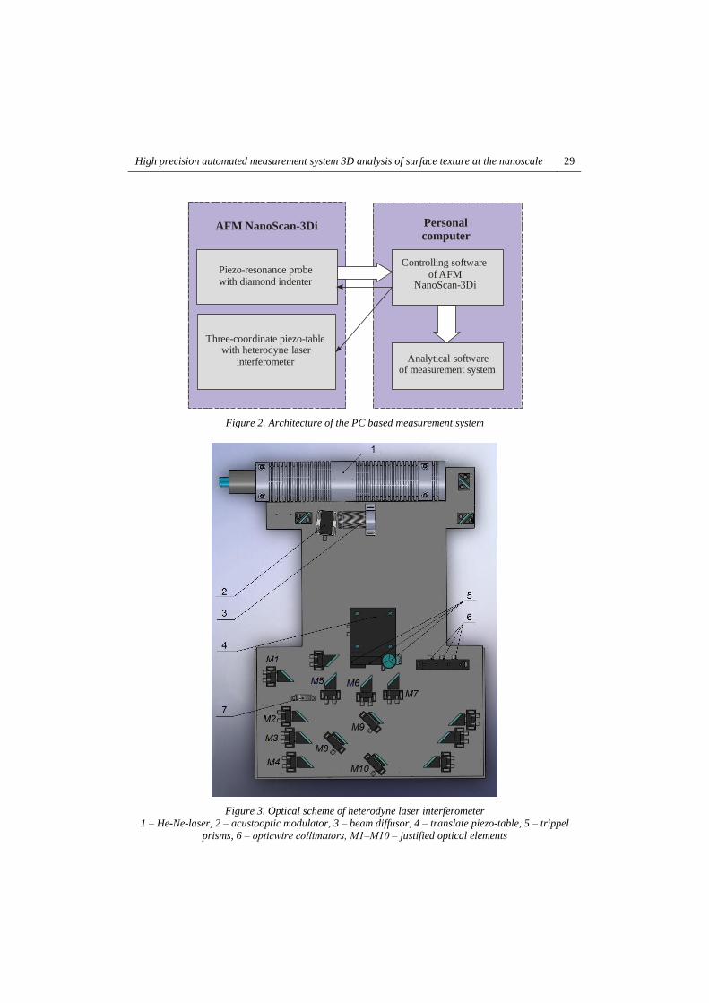
Measuring system has a module architecture that is shown in Figure 2. It consists of the
atomic-force microscope, the high range coordinate table and a personal computer with
controlling software and analytical software.
The central element of this system is the atomic force microscope NanoScan 3Di having
piezo-resonance probe with stiff console and solid mechanical indenters made of artificial
diamonds.
Scanning of the surface texture implies horizontal movement of the specimen by means
of three-coordinate table. Parametrical analysis of nanostructure texture imposes extended
requirement to the horizontal range of the table. That is why system includes specially

28 Valery Poroshin–Dmitry Bogomolov–Oleg Poroshin–Valery Lyssenko
constructed high range and high precision three-coordinate piezo-table equipped with
heterodyne laser interferometer having digital phase detector (Figure 3).
Table 1
Main properties of the measurement systems
Property Description
Measurement principle Atomic force microscopy
Probe type Diamond indentor
Horizontal range (um) 500
Vertical range (um) 50
Horizontal resolution (nm) < 0,1
Vertical resolution (nm) < 0,1
Time resolution of measurements (ms) 1
Max. measurement speed (um/s) 30
Axis orthogonality error (rad) 0,01
Digital filtering 3D Gaussian
Measured parameters
Sa, Sq, Sp, Sv, Sz, Ssk, Sku, Sdq, Sdr,
Sal, Str, Std, Smr, Sdc, Sxp, Vmp,
Vmc, Vvv, Vvc, Spd, Spc, S5p, S5v,
S10z, Sda, Sha, Sdv, Shv
Figure 1. High precision PC based measurement system for a 3D surface texture analysis
at the nanoscale
High precision automated measurement system 3D analysis of surface texture at the nanoscale
29
Three-coor heterodyne
interferometer
dinate piezo-table with laser
Piezo-resonance probe with diamond indenter
AFM -NanoScan 3Di
C of AFM
NanoScan-3Di
ontrolling software
Analytical software of measurement system
Percomputer
sonal
Figure 2. Architecture of the PC based measurement system
Figure 3. Optical scheme of heterodyne laser interferometer
1 – He-Ne-laser, 2 – acustooptic modulator, 3 – beam diffusor, 4 – translate piezo-table, 5 – trippel
prisms, 6 – opticwire collimators, М1–М10 – justified optical elements

30 Valery Poroshin–Dmitry Bogomolov–Oleg Poroshin–Valery Lyssenko
Electronic module of the three-coordinate table has time resolution of 1 ms that allows
to perform surface scanning at up to 30 um/s speed. Measured data are transferred to the PC
by means of USB interface.
Controlling software provides preliminary probe placement, motion control of table and
probe, performing of single point measurement and incorporation of measured data into
unified digital field.
After the measurement process is finished measured data are transferred to the
analytical software. Analytical software implements surface visualization, form filtering
(including specimen slope levelling), frequency filtering by means of digital phase-
corrected Gaussian filter, parametrical assessment, correlation analysis and surface curve
analysis. Parametrical analysis includes 28 parameters that are divided into groups of
amplitude and hybrid parameters, spatial parameters, functional parameters, and
segmentation parameters.
A number of preliminary measurements of the 3D surface texture were carried out to
test the measurement system applicability. The preliminary measurements include
calibrating lattice measures TGT and TGZ, diamond surface, grained surface and plasma
processed surface. Example of the 3D analysis of the amplitude surface texture parameters
of the grained surface and diamond surface in analytical software are presented in Figure 4–
10.
The Sz (maximal surface texture height) values obtained during the analysis are equal to
the nominal lattice values of TGZ and TGT. Combination of Sp (highest surface peak) and
Sv (deepest surface valley) parameters is always equal to Sz.
Figure 4. Sample of 3D surface topography of the grained surface

High precision automated measurement system 3D analysis of surface texture at the nanoscale
31
Figure 5. Sample of 3D surface topography of the grained surface
Figure 6. Sample of 3D surface topography of the grained surface

32 Valery Poroshin–Dmitry Bogomolov–Oleg Poroshin–Valery Lyssenko
Figure 7. Sample of 3D surface topography of the grained surface
Figure 8. Sample of 3D surface topography of the grained surface

High precision automated measurement system 3D analysis of surface texture at the nanoscale
33
Figure 9. Sample of 3D surface topography of the grained surface
Figure 10. Sample of 3D surface topography of the grained surface

34 Valery Poroshin–Dmitry Bogomolov–Oleg Poroshin–Valery Lyssenko
The Sa (arithmetic mean texture height) and Sq (root-mean-square texture height) are
approximately similar and equal to 30–50% of Sz. The Sdr (developed interfacial area ratio
of the scale-limited surface) is always exceeding 100%. It is minimal for the least height
surface (calibrating lattice measure TGZ01).
So, preliminary results of the surface texture analysis of calibrating measures and real
nano-surfaces allows to suggest that the described measurement system is suitable for
providing the surface texture assessment at the nanoscale.
3. Conclusion
Proposed measurement system provides automated high precision measurements and
complex PC based parametrical 3D analysis of surface texture at nanoscale. It can be
recommended to use in modern nanotechnology and precision engineering laboratories.
The research was performed with the financial support of the Ministry of Education and
Science of the Russian Federation for higher education institutions within the state job
service.
4. References
[1] Whitehouse, D. J. Handbook of Surface and Nanometrology. Second Edition, CRC Press, 2010,
pp. 999.
[2] Geometric Product Specification (GPS) – Surface texture: Profile method – Terms, definition and
surface texture parameters. International Standard ISO 4287:1997.
[3] Geometric Product Specification (GPS) – Surface texture: areal – Part 2: Terms, definitions and
surface texture parameters. International Standard ISO 25178-2:2012.
Design of Machines and Structures, Vol 4, No. 2 (2014) pp. 35–44.
MESOSCOPIC LATTICE-BOLTZMANN MODELLING OF FLOW IN THIN CHANNEL WITH ROUGH WALLS
VALERY POROSHIN–DMITRY BOGOMOLOV–ANNA ANOSOVA– VICTOR RADYGIN
Moscow State Industrial University of, Science Department 115280, Avtozavodskaya st. 16, Moscow, Russia
Abstract: The mesoscopic mathematical model of flow in thin channel with rough walls in the 2D approach is proposed. The model is based on the lattice-Bolzmann numerical method. The measured roughness profiles were used in numerical experiments. The effect of the surface roughness upon leakage is shown. Keywords: thin channel, surface roughness, Navier-Stokes flow, lattice-Boltzmann
1. Introduction
Designing of the new mechanical components and technical elements for modern industry often states the problem of providing the desirable hermiticity of thin gaps or regulating the flow through thin channels. Flow pattern in such thin layers significantly determines total efficiency of developed machines and devices.
Main factors, which have a great influence upon the leakage in thin channels of machine components, include interaction characteristics, physico-mechanical properties and geometry of the channel. Roughness of the channel surfaces is also one of the main factors, which have a great impact on leakage.
In authors’ earlier works some numerical models of the lubrication flow in the immovable and moving seals with rough walls were proposed [1, 2]. The flow factors were offered for considering the surface roughness effect. The detailed analysis of the surface roughness influence upon the seal hermeticity was presented.
But the lubrication flow model based on the common Reynolds equation is associated with essential restrictions on the physical features of the media and the flow patterns. For example it implies laminar flow with very low Reynolds numbers (Re should not surpass 10–20). Such restrictions significantly shorten the possible range of considerable mechanical components, especially with moving walls.
Present work introduces a new numerical lattice-Boltzmann model of the flow in the thin channels with rough walls. Accepted numerical method allows to turn to the Navier-Stokes approach which has much less physical limitation than lubrication flow approach. So, proposed model allows to examine the influence of the surface roughness upon the flow in the thin channel in Navier-Stokes approach.
2. Mesoscopic flow model
The geometry model of the thin channel formed by two rough surfaces h1, h2 is presented in Figure 1. The average gap between two rough surfaces (H) is taken as the distance between their mean lines. Upper and lower walls has coordinates
xhHxH 11 )( and xhHxH 22 )( . The current gap in the channel is calculated as xhxhHxhT 21)( .

36 Valery Poroshin–Dmitry Bogomolov–Anna Anasova–Victor Radygin
hH
QH/2
H/2
H
H
h
h
x
y
U
22
T
11
Figure 1. Geometry model of the thin channel with rough walls
Measured profiles of the real industrial surfaces or simulated roughness profiles with desirable features can be used as a surface geometry. Both profiles are always specified on regular grid with Δx step.
For the lattice-Boltzman modelling the square shape numerical lattice δx = δy should be introduced on the channel geometry model. Numerical lattice step is considered as some fraction of the profile grid Δx = kδx where k is an integer value.
The common Navier-Stokes equations are frequently used as a model of viscous flow of a laminar Newtonian media. For the viscous gas in vector notation they are:
SdivudivppgradFdt
du 2)(3
2)(
,
0 udt
d
, (1) where u is the flow velocity, ρ is the media density, p is the pressure, µ is the media
viscosity, S is the stress deviation tensor, F represents body forces. There are three traditional ways of solving the Navier-Stokes equations – finite
difference method, finite element method and finite volume method. All traditional methods have some significant problems dealing with curved boundaries.
That is why the alternative lattice methods are widely applied for the flow modelling in modern investigations. They use the representation of the flowing media as a composition of particles interacting on the discrete lattice. Implementation of the fundamental conservation laws, laying in the base of Navier-Stokes equation, guarantees them correct results. Some lattice methods deals with microscopic interactions of single particles in the lattice nodes. Other methods use mesoscopic approach implying the particle distributions in each lattice node.

Mesoscopic Lattice-Boltzmann modelling of flow in thin channel with rough walls
37
Lattice-Boltzmann numerical method is a general lattice method based on the
mesoscopic Boltzmann transport equation. If we consider f(r, v, t) as a particle distribution by particle velocity v in each r(x, y, z) point at the time moment t, the Boltzmann equation has a form of:
dtdvdrfdvdXtvrfdvdrdttFdtvvdtrf )(,,,,
yy
xxyx v
fF
v
fF
y
fv
x
fv
t
f
,
)( fv
fF
r
fv
t
f
, (2)
where Ω is the collision operator, characterizing the physical conditions of the media. In 2D case Boltzmann equation is expanded as:
yy
xxyx v
fF
v
fF
y
fv
x
fv
t
f
. (3) Local flow characteristics at each point are calculated by integrating of the particle
distribution:
dvtvrfmtr ),,(),(,
dvtvrfvmxrtutr ),,()(),(,
dvtvrfvmtr
tru ),,(),(
1),(
,
dvtvrfuvmtretr ),,(2
1),(),(
2,
dvtvrfuvmtr
tre ),,(),(2
1),(
2
(4) where m is generalized particle mass, e is the intrinsic energy. For isothermal flow the e = const condition should be used. The Bhatnagar-Gross-Kroor (BGK) collision operator is commonly used for simulating
the viscous Navier-Stokes flow. It reduces the particle distribution to the equilibrium distribution, defined by Maxwell-Boltzmann equation:
2
22
230 /)uv(exp
n)v(f
/ , (5)
where 32 /eTkB is the generalized temperature, m/n is the local
particle amount. Simple BGK approximation is a time relaxation operator:
01ff
, (6)

38 Valery Poroshin–Dmitry Bogomolov–Anna Anasova–Victor Radygin
Substituting BGK approximation (6) the Boltzmann equation (3) should be transformed as:
01ff
v
fF
v
fF
y
fv
x
fv
t
f
yy
xxyx
. (7)
As shown in Chapman-Enskog analysis [3], the Boltzmann equation with BGK collision operator (7) is equal to the Navier-Stokes equation (1) for uncompressed fluid or slightly compressed gas when the Mach number is small and the flow is isothermal.
3. Calculation model
According to the numerical lattice-Boltzmann method the calculation process is simulated as a sequential evolution of the flow on the discrete lattice. During the streaming step all particles are migrated to the neighbouring nodes in all possible directions. Particles that appeared in the same node take part into the collision step. Converging iterative process describes the stationary flow behaviour.
In present research the D2Q9 discrete lattice was chosen for the numerical simulations. This lattice assumes migration of particles in 4 straight and 4 diagonal directions as shown in Figure 2. The zero-migration discrete direction (node 9) is also implied.
9 1
234
5
6 7 8 Figure 2. Lattice-Boltzmann D2Q9 numerical lattice
Straight discrete movements implies discrete particle velocities of absolute value cv i where c = δx/δt is a lattice constant (lattice sound speed) and δt is the time step.
Diagonal movements implies greater velocities of absolute value cv i 2 . The resulting discrete velocity vector is calculated as:

Mesoscopic Lattice-Boltzmann modelling of flow in thin channel with rough walls
39
9),0,0(
8,6,4,2,24/)1(sin,4/)1(cos
7,5,3,1,4/)1(sin,4/)1(cos
i
icii
icii
vi
. (8) The continuous particle distribution function is also substituted by a set of discrete
distribution functions:
),(,,( trftvrf ii . (9)
The streaming step is simulated as:
iitxii Ftrftvrf ),(),( . (10)
The collision step equation can be expanded from the continuous Boltzmann equation with BGK approximation (7):
tititi trfuftrftrf
,,,1
),(),(' 0
, (11)
where x / is the discrete relaxation parameter, f’ is the new particle
distribution after the collision step. Local quantities Local flow characteristics implicated in the equation (11) in discrete form are calculated
by transforming integral to sum:
i
ifn,
i
ifm,
iii
iii
fv
fvmu
. (12) Discrete equilibrium particle distribution for the isothermal flow is calculated as shown
in [3, 4]:
uu
cuv
cuv
cnwf iiii 2
2
420
2
3
2
931
, (13) where wi are the specific weight coefficients. For the D2Q9 lattice they are defined as:
.9,9
4
,8,6,4,2,36
1
,7,5,3,1,9
1
i
i
i
wi
(14) The local conservation laws are also true for the equilibrium distribution:
i
ifm 0
,
ufvmi
ii 0
(15) While using numerical lattice methods, standard macroscopic boundary conditions
should be converted to the mesoscopic terms (specific particle distributions and collision operators on the boundaries).

40 Valery Poroshin–Dmitry Bogomolov–Anna Anasova–Victor Radygin
For the solid wall boundaries of the channel the no-flow and no-slip macroscopic
boundary conditions should be implemented. As a mesoscopic alternative, the classic “bounce-back” boundary scheme [4] was used in present research. In “bounce-back” boundary nodes are not the part of the flow and special collision operator is defined them. All the particles, arrived to the boundary node on the streaming step are just mirrored in the opposite directions on the collision step:
),(),('* tbitbitrftrf
, (16) where rb means boundary node coordinates, i* is the direction opposite to i direction. For the open boundaries of the channel there are two ways of defining boundary
conditions. The first way is to define flow velocity boundary conditions:
IuConstu on the channel inlet, 0ˆ/ xu on the channel outlet. (17)
Here is the mesoscopic interpretation of flow velocity boundary conditions:
IitiIittiIitIiuv
cvrwtvrftrf ***** 2
32),(),('
),(),(' ttrftrf fitOi
. (18) where rI is the inlet boundary node, rO is the outlet boundary node, rf is a flow node
adjacent to the rO. The second way is to define strict p boundary conditions:
Ipp on the channel inlet,
Opp on the channel outlet. (19)
On the mesoscopic level constant pressure on the boundaries means constant ρ because p = cs
2ρ. The equilibrium particle distributions with zero velocity are used for boundary conditions:
2s
iBi cm
wpf
. (20) where pB is the pressure on the specified open boundary node. After the lattice-Boltzmann calculation is finished the resulting local flow
characteristics could be calculated by (12). Then the integrated flow characteristics could be calculated.
Total leakage through the channel was calculated as an integrated horizontal velocity of the local flow on the channel outlet:
xj
J
jxx yLuBQ ),(
1
(21)
where B is the channel thickness, L is the channel length. The flow factor φx was also calculated, that shows the decrease of Qx in comparison to
the smooth wall channel with the same geometry Qx*:
L
ppHBQ BA
x 12
)(3*
, */ xxx QQ. (22)

Mesoscopic Lattice-Boltzmann modelling of flow in thin channel with rough walls
41
4. Analysis
The computation software were developed for the proposed numerical model and the
numerical experiments were carried out. The results achieved for the smooth wall channel are shown in Figure 3.
near open boundaries
inner section
Figure 3. Vertical section of ux for channel width smooth walls
The well-known feature of the flow in the smooth wall channel is a parabolic distribution of flow velocity in the vertical section of the channel. Strict parabolic distribution was achieved in LBM simulation for the inner sections of the channel. Some transient process was achieved near the open boundaries. They are due to the constant boundary conditions on open boundaries. The other well-known features of the flow in the

42 Valery Poroshin–Dmitry Bogomolov–Anna Anasova–Victor Radygin
smooth wall channel (negligible vertical pressure gradient and vertical velocity, linear pressure distribution along the channel length) were also granted in numerical simulations. In complex they validate the numerical model correctness.
Other numerical experiments were carried out for the rough wall channels. In Figure 4 two different rough surfaces are shown. The first one is the surface after the grinding with low roughness height. The second one is the surface after milling with greater roughness height. The length of the analysed channel was 0,8 mm.
surface after grinding
surface after milling
Figure 4. Surface roughness profiles
Typical flow velocity distribution in channels with both grinded and milled surfaces is shown in Figure 5. The local velocity significantly increases where the channel is narrowed. In vertical section the flow velocity still has parabolic distribution. Also the increase of vertical flow velocity near the channel narrowing zones was achieved. It is due to the streamlining of the roughness peaks.
The resulting values of the flow factors in channel with different surface roughness profiles are shown in Figure 6. The results are shown as a graph showing the flow factor evolution while growing of the average gap from 7 to 12 um. For the more thin channels the flow factor values are more significant, i.e. the roughness influence is more strong. Regular surfaces with great roughness height show stronger influence.

Mesoscopic Lattice-Boltzmann modelling of flow in thin channel with rough walls
43
surface after grinding
surface after milling
Figure 5. Flow velocity in channels with rough walls

44 Valery Poroshin–Dmitry Bogomolov–Anna Anasova–Victor Radygin
Figure 6. Evolution of the flow factors with growing of average gap H
At the same time, the small roughness surfaces allow to achieve lesser values of average gap and so decrease leakages.
5. Conclusion
Proposed model can be used to forecast leakage in thin channels with rough walls in the Navier-Stokes approach. Small roughness height should be combined with regular surface texture to decrease the resulting leakage.
The research was performed with the financial support of the Ministry of Education and Science of the Russian Federation for higher education institutions within the state job service.
6. References
[1] Poroshyn, V. V.–Bogomolov, D. G.: Application of finite element method (FEM) for calculation of flow factors in seals. International Journal of Applied Mechanics and Engineering, 2002, Vol. 7, No. 3, pp. 961–972.
[2] Shejpak, A.–Poroshin, V.–Syromiatnikova, A.–Bogomolov, D.: Roughness influence upon the hermiticity of plunged pair using equivalent gap model. Advanced Engineering, (2008) No. 2, pp. 283–290.
[3] Wagner, A. J. A practical introduction to the Lattice Boltzmann method. North Dakota State University, 2008.
[4] Mei, R.–Luo, L. S.–Shyy, W.: An accurate curved boundary treatment in the Lattice-Boltzmann method. ICASE report No 2000-6. Langley Research Center, 2000.

Design of Machines and Structures, Vol 4, No. 2 (2014) pp. 45–52.
THE SATELITE-BASED ALGORITHM FOR DETERMINING THE LOCATION OF HYDRAULIC LIFT
ANATOLY SHEIPAK–PAVEL NOVIKOV Moscow State Industrial University
115280, Avtozavodskayast. 16, Moscow, Russia [email protected], [email protected]
Abstract: The article describes the specialized complex system for the hydraulic lift location determining. System consists of INS, Glonass and odometer. The advantages and disadvantages of used navigation systems are observed. The different error correction methods are also considered. Keywords: acceleration, satellite, error model, gyro drift, odometer
1. Introduction
The fast development of technology for the last ten years has shown a great opportunity for successful solution of different navigation tasks, with the help of different devices that can be sat on the board of any craft or outside it. These tasks are actual not only in aviation, missiles, fleet, but also on the ground transport. But the high price is a reason why people cannot use them everywhere.
2. Statement of the problem
There are two different ways to calculate the way, inertial navigation systems (INS) and Glonass. An Inertial navigation system is a system of sensor designed to measure specific force and angular rates with respect to an inertial frame which, when integrated, provide velocity, position and attitude.
There are two approaches for the navigation frame simulations in the inertial system technology. The first one deals with the physical implementation of the navigation frame using a three-axes gyro-stabilized platform with three orthogonally placed accelerometers. Such type of a system is called INS platform.
The second one, called INS strapdown, provides the analytical image of the navigation frame in an on-board computer, using measurements from accelerometers and rate gyros installed directly on a vehicle body. The platform creates navigation frame on the board of the object, due to which it is possible to define the parameters of motion.
The principle of Glonass working differs from INS working. Glonass is a network of about 24 satellites orbiting the Earth. Wherever you are on the planet, at least 4 satellites are visible at any time. Each one transmits information about its position and the current time at regular intervals. These signals, travelling at the velocity of light, are intercepted by your Glonass receiver, which calculates how far away each satellite is based and how long it takes the messages to arrive.
In general, the Glonass signal contains pseudorange, carrier phase and Doppler measurements. The pseudorange and Doppler measurements can be utilized for position and velocity calculation; these measurements are typically in high sensitivity receiver applications. Pseudrange observations are obtained by measuring the transit time of the signal as it travels from Glonass satellite to the receiving antenna.
Due to non-synchronized receiver and satellite clocks, the measured range (pseudorange) is biased. Therefore, the receiver’s clock difference with respect to the

46 Anatoly Sheipak–Pavel Novikov
satellite’s Glonass time must be taken into account. This leads to a system of equations with four unknown parameters (three coordinates and clock drift); thus at least four satellite observations are necessary for position calculation.
A Glonass receiver calculates its position by precisely timing the signals sent by Glonass satellites high above the Earth. Each satellite continually transmits messages that include time the message was transmitted and satellite position at time of message transmission.
The receiver uses the messages to determine the time transmission of each message and calculates the distance up to each satellite using the velocity of light. Each of these distances and satellites locations defines a sphere. These distances and satellites locations are used to calculate the location of the receiver using the navigation equations. Mistakes don’t accumulate during their work.
Glonass orbital errors occur due to the differences in the actual and modelled positions of the satellites. Three types of data, of non-uniform accuracy levels, are accessible for position and velocity determination of the Glonass satellites: almanac, broadcast ephemerides and precise ephemerides. Broadcast ephemerides are available in real time and orbital parameters are uploaded for each interval of two hours.
Figure 1. Principle of Glonass working
Another type of error is satellite clock error. These errors are due to the offsets in the clock frequency of each satellite with respect to the reference clock, which is monitored by the Master Control Station. The satellite error is usually less than 1 ms and, after implementing the broadcast correction, the remaining error is in the order of 8 to 20 ns (2 to 3 m). This error can be eliminated by D Glonass (difference in between the receivers), since it is the same for all receivers in the proximity, subject to essentially identical signal paths, simultaneously tracking the same satellite.
Both methods have advantages and disadvantages. INS systems errors are large in magnitude, low frequency in nature and grow over time. These error qualities stem from the solution of the second order differential mechanization equation. INS errors can be divided into two parts. The first is the stationary component (e.g. gyroscope drifts, horizontal attitude errors) which is independent of motion parameters and yields those INS errors oscillating over time with a very small Schuler frequency corresponding to a period of 84,4minutes. Therefore, this large component is quite predictable from an estimation point

The satelite-based algorithm for determining the location of hydraulic lift
47
of view and, thus it can be compensated in the output. The second non-stationary class of errors (e.g. sensor scale factors, installation errors and azimuth misalignment) is defined by motion parameters (vehicle accelerations and velocities, travelled distance), which makes it different to predict. The advantage of inertial systems is there autonomous working, all calculations are made on the board of the craft.
The universal system, which can work with all kinds of objects, doesn’t still create. That’s why the creation of system, which allows to use extra information about motion is relevant. The source of this information can be odometer – the device which counts the way. Odometer counts the rotation of wheel and conversion this to the value of the traversed path. There are several automobile systems, which include odometer. Unfortunately most of these systems exist like a prototype. High price and low accuracy doesn’t allow produce them serially. That’s why the creation of low cost system, which able to determine the position of the object with a given accuracy is still topical. INS errors determined by the accuracy of using sensors. The gyro drift is a very important parameter. If we use these systems on the Earth we can get information about velocity using odometer. Thus there is no need to count these velocity using INS systems.
However, both systems have a number of limitations which challenge their use in many land-based applications. Inertial sensor errors, for example, can be large in magnitude and grow over time without compensation using external information such as Glonass. On one hand, widespread use of a very accurate INS is constrained by their high cost. On the other hand, the operational capability of Glonass degrades in harsh environments such as urban and forest areas, where Glonass signal may be partially or completely blocked by buildings and dense foliage. Glonass receiver does not provide attitude information. The combination of Glonass and INS is well suited to the development of a range of applications as each unit compensates for the other’s shortcomings.
Figure 2. Configuration of orbital grouping system Glonass
The combination of Glonass and INS can deliver superior system performance in comparison to the performance of either system in stand-alone mode. One important

48 Anatoly Sheipak–Pavel Novikov
advantage of an INS is the ability to provide attitude data in addition to position and velocity information. The data rate of GPS measurements is typically 1–20 Hz, while the INS data rate is 60–100 Hz on average.
Despite above advantages, system inaccurate due to gyro drifts and accelerometer biases cause a rapid degradation in position quality, while Glonass errors are generally smaller and are not time-dependent. A Glonass receiver has high frequence errors while an INS typically does not. The differences in the nature of errors associated with the two systems benefits their integration through the use of a Kalman filter, which is a linear estimator that uses knowledge of the system dynamics and external measurements to obtain an optimal estimate of the state variables at the current epoch. It follows, therefore, that these two units combined in a common system will provide superior operation in terms of accuracy, integrity and availability than each system in stand-alone operation.
The problem of achieving better performance in terms of accuracy of INS/Glonass systems can be divided into two distinct problems: modeling and estimation. The modeling problem is concerned with the development of error models that describe more accurately the INS/Glonass system. The estimation issue devoted to achieving moro accurate error estimates, which are used for error compensation, trought the proper of the available process and measurement information. However, there is a contradiction between the two issues, since excessive complication of a system degrades the estimation accuracy of the state vector components. To achieve optimal results, a balance of two approaches should be attended.
Although recently a wide variety of different estimationalgorithms have been investigated for INS/Glonass integration. Kalman filter techniques are still more commonly applied for many applications. From the estimation viewpoint, the optimality of a conventional Kalman filter requires, in principle, good a priori knowledge about the process and noise statistics as well as a sufficiently long estimation time or data length. If the above information is inaccurate or varies in a manner that is not readily predictable, the estimation accuracy degrades from the theoretical prediction. These criteria have limited the applicability of the traditional Kalman filter in the case of INS/Glonass systems, both conceptually and practically. Adaptive filters and smoothing techniques sense the properties of the environments in which they operate and adjust the filter parameters accordingly. Therefore, when the properties of the operating environments are not known, or when they change with time in a previously unknown manner, these filters become very useful. Thus, such estimation methods are beneficial for INS/Glonass integration in changing Glonass conditions.
Several different integration schemes have been developed in recent years. They can be divided into two types: loosely coupled (sometimes referred to as centralized) and tightly coupled (referred as decentralized) strategies. In centralized schemes all measurements from INS and Glonass are processed in the same filter. The main advantage of this technique is in preserving data integrity. When there are less than three satellites observable and Glonass receiver does not provide any navigation solution, the pseudorangels of the remaining satellites can be used for a measurement update.
Another benefit of this type of integration comes from the fact, that poor Glonass measurements can be detected and rejected from the solution. However, tightly coupled algorithms usually have a sophisticated system model; consequently, large dimensions of the state vector degrade the estimation accuracy. The decentralized approach has become more popular for many applications. This method is based on the independence of the

The satelite-based algorithm for determining the location of hydraulic lift
49
Glonass and the INS navigation functions. It is a simple and flexible approach, since the filter size is relatively small compared to the extended Kalman filter in the tight integration. The only limitation of the loosely coupled integration scheme comes from the fact that at least four satellites are necessary to provide Glonass updates for the INS filter.
The high price of INS/Glonass system doesn’t allow to produce it. The main goal now is to create a complex cheap system that consists of INS and Glonass with less accurate sensors and creation of data processing algorithm providing the specified accuracy. The main idea of the working system is alternately switching of INS and Glonass.
Error correction of INS by uses classic algorithm from Glonass receiver can be done with the help of the closed method. It is based on the application of additional control actions to the real or imaginary system platform. This system can be done only if for arbitrary motion can be allocated in the output values of the inertial velocity and . To avoid errors, we can apply external sources of information about the speed. If we have eastern and northern components of the velocity of the object due to Glonass, then up to its own satellite system errors:
δVe Ve VEG , (1)
Damping-K1δV control signal is input to the velocity calculation unit of the navigation algorithm. The single channel error model has a form (E-channel):
δVE gФN δfE K δVE, ФNVE
RδωN K δVE, (2)
Differentiating the first equation and substituting the second in his right part, we obtain the variation of error :
δVE K δVE RK g δVE gδωN δfE, (3)
From the last equation it follows that the error in the output data decreases subsequently time, and the frequency
ω ν K g ν, (4)
Figure 3. Closed method of error correction
The open method uses special algorithms for estimating errors of uncorrectable (autonomous) inertial system, which can be based on a priori information about their character, as well as the measurement of object motion parameters using external devices,

50 Anatoly Sheipak–Pavel Novikov
including Glonass receiver and odometer. The most common and effective algorithm of this kind is the optimal Kalman filter.
Let us consider any linear system that can be described by certain values usually inaccessible for the measurement. These values are elements of state vector dopted a linear variation of the system (model):
x Фx Gw (5) whereФ is the transition matrix, G is the input matrix, is the input white
noise with covariance matrix Q. The parts of the state vector components or their linear combinations are directly
observable according to the equation: z Hx v , (6) where is the measurement vector; is the measurement white noise with zero
meaning and known covariance matrix R. Kalman logic allows to obtain the best estimation of the system, based on the
measurement with errors. The Kalman filterprovides minimization of the mean-square error.
J TrM x ξ x ξ T min. (7) At the first stage of applying the algorithm creates a priori estimate of the state
vector of the system based on the assumption that the adopted model is accurate and contains no input noise:
Ф (8) When the next value of the measurement vector obtained, it is possible to specify a
priori estimate by introducing feedback changes with matrix : ξ =ξ +K z Hξ . (9)
Figure 4. Open method of error correction
The second stage of the application filter algorithm includes finding the optimal value of the matrix in accordance with the selected criteria:
0, (10)
. (11) where is the covariance matrix of
estimation errors, which can be calculated: Ф Ф . (12)

The satelite-based algorithm for determining the location of hydraulic lift
51
Then we can calculate covariance matrix:
(13) If we cannot find measurement vector then Kalman filter is put on prediction
mode. For example, take R=∞ and then, according to the above described sequence of operations, the state vector estimation is performed using only a single model, and coincides with the a posteriori estimation of the a priori:
Ф (14) Concurrently with the main estimation function Kalman filter allows to smooth the
noise contained in the measurement vector . The principle of open inertial correction relies on the definition of its errors. So, for the
eastern channel platform inertial obtain: δEδVEФN
δωN
1 T 0 00 1 – gT 0
0 T
R 1 T
0 0 0 1
δEδVEФN
δωN
000T
w (15)
1 0 0 00 1 0 0 Ф (16)
Knowing at each step of calculating the value , and applying the Kalman filter, we can estimate the errors of the inertial system, including those that are not available for direct measurement (in particular, the deviation Ф platform from the horizontal plane and angular velocity its drift).
Figure 5. Integration scheme of INS, Glonass receiver, odometer
These estimates are used to amend the output readings of the coordinates , , , velocity , , and orientation angles Ψ , , .

52 Anatoly Sheipak–Pavel Novikov
In practice creates different combination techniques to correct the INS output data
combining dignity closed and open circuits. One such techniques use information from Glonass receiver, inertial navigation system and odometer. In fact this method repeats the classical scheme of integrated inertial navigation system: errors of the inertial system are evaluated in real time using a Kalman filter, the obtained estimates are used for damping of physical or imagined platform, and to amend in the output data of the system.
This method extended by using the information from odometer. On the one hand they allow to identify and compensate the residual error of azimuthal alignment, on the other - to implement forecasting errors of the inertial part during the absence of high-quality reception of signals from navigation satellites, because odometer measurements are always available. The comparison of the distance traveled, calculated by the Glonass and odometer allows to calibrate the scale factor.
However, there are several reasons impeding of incarnation of described scheme. First of all it is low accuracy of micromechanical sensing elements. It does not allow such testimony to the coordinates and velocity which errors would submit to linear law. Unfortunately we can’t use more expensive primary information sensors in this system because the price of the whole system will rise up.
Moving transport occurs in a narrow space, so very often satellite signal disappear, in these circumstances, the most reliable source of information about traversed path speed is odometer. All that means, that we have to develop specialized alternative algorithm of synthesis of navigation information, which we can get from different sources.
3. Conclusion
This paper proposes an alternative approach procedure to evaluate location settings land mobile objects that require precise positioning. The proposed system is fundamentally differs from existing, one because it is based on sensitive elements having a small size, and low market price. The proposed algorithm analysis of the system was tested in actual operating conditions.
4. References
[1] Salychev, O. S.: Applied Inertial Navigation: Problems and Solutions – M. BMSTU Press, 2004. [2] Vlasenko, A.: Integrated gyroscopes iMEMS – angular velocity sensors of Analog Devices firm /
Electronic Components, 2003. [3] Hemerly, E. M.–Schad, V. R.: Implementation of a GPS/INS/Odometer. 2008. [4] Hong, S. K.–Park, S.: Minimal-drift Heading Measurement using a MEMS Gyro for Indoor
Mobile Robots // Sensors. 2008, Vol.8, pp. 7287–7299. [5] Smart – V1 Antenna. Data Sheet. Version 0D [Electronic Resource] – NovAtel Inc., 2006.

Design of Machines and Structures, Vol 4, No. 2 (2014) pp. 53–58.
GENERATING CONCEPTS WITH THE HELP OF GREEN TIPS
ÁGNES TAKÁCS
University of Miskolc, Institute of Machine and Product Design
3515, Miskolc-Egyetemváros
Abstract:Conceptual design is the early phase of the whole design process where the designer
engineer analyses the similar on the market existing products, complete them with his or her own
ideas and generating new solutions this way. In a lucky situation the designer can generate all the
possible solutions of the product. In this case analysing solutions is a really hard task and in many
cases cannot be solved without the help of a computer. This paper introduces a previous work
integrated by the tools of environmentally friendly design.
Keywords: design theory, methodology, Design for Environment
1. Introduction
Due to the literature of the field environmentally friendly design or DFE or Green
design or eco design mean only the protection of the nature do not pay any attention to the
protection of the human that is a component of the green environment, only indirectly
referring to it. It is essential to notice that the man only as a designer but also as the part of
the green environment appears in the machine-human-environment cycle. The elements of
the cycle are interrelationship continuously. So the human designs for itself and for the
environment as well. Machine has the effect for the human and for the environment too.
The environment also has the impact for the human and for the machine. So environment
means not only the nature over the office, the factory, but the direct environment of the
human where it works, so the workplace. As for the further researches it would be practical
to mention and analyse ergonomics as the element of the environmentally friendly design.
2. Tools of DFE
2.1. DFE elements
Dfx, or design according to a given viewpoint [2] can be any formal period of the
design process, or any important aspect that can be followed during the whole design
activity as the main principle. Dfx is an enormous set of design principles that is really hard
to describe, because this set is increasing day-by-day. Scientists define more and more
principles, and for those principles methods are also created. These methods denote or can
denote the adaption of Dfx techniques to computer. DFE, that is Design for the
Environment is collecting the aspects of environmentally friendly design. It consists of
seven essential areas: design for recycling, design to minimize material usage, design for
disassembly, design for remanufacturing, design to minimize hazardous materials, design
for energy efficiency, design to regulations and standards. According to different aspects
these can be divided into other different principles. This figure also confirms why it is so
complicated to collect all the Dfx techniques and to group them.

54 Ágnes Takács
2.2. 3R, 4R, 6R
3R philosophy means nothing else but not accumulating used or consumed materials as
waste, but recycling them to the product-market. Reduce means to lower the quantity of the
waste, reuse means using again the waste, recycling means using waste for creating new
raw material. There are several versions for 4R. Usually recover, rethink and replace are
mentioned as the 4th R.
Elements of 6R are recycle, reuse, repair, replace, reduce, rethink. Rethinking a product
can lead to an absolute green product, for instance using biodegradable materials. Of course
it determines and might lower the life-time of the product (e.g.: plant-a-tree box, as a
packaging carton box, patent no.: US20080046277A1). But this way the effect on the
environment can be reduced the most. Reducing the waste cannot be the best solution, as
even though making the quantity of the waste less, it still has the impact on the
environment. During redesign certain assemblies can be changed by less harmful ones.
Repairing a product that is out of order its lifetime gets longer, so less new product is
needed. It is sure that this possibility is not proper for the manufacturers. Reusing a product
is significant for the environment. Due to recycling less natural raw materials have to be
extracted. The recycled raw material has no impact on the environment as waste, but the
recycling procedure might be dangerous for the environment. It does not mean to be worst
than extracting the natural materials.
2.3. Valdez or CERES principles
There are several principles that were defined to make the industry understand and deal
with the effects of producing for the environment. For example Valdez principles that were
published in the Financial Times 27th March 1991. These principles later had been
renamed for CERES principles. Coalition for Environmentally Responsible Economies had
been established by Joan Bavaria in 1989 that is the abbreviation for CERES, who was the
Roman goddess for fertility and agriculture. After the Exxon Valdez oil spill in the same
year of establishing, CERES determined its 10 point principles. These help factories
producing with the highest environmentally efficiency. Many industries keep CERES
principles in front of the eye nowadays, General Motors among others.
2.4. Ten Golden Rules
Ten golden rules were carried out by Luttropp and Lagerstedt [1]. The rules are the
summary of those principles that are used by different industries, and suggested by hand
books. Ten golden rules are quite general; each industry should carry out product and
industry specific rules.
2.5. Life cycle assessment
Figure 1 shows the stages of the product lifecycle in the point of view of the material.
The process starts with the extraction of the raw material, with that the production of the
stock can be started. From the stock products are prepared. These products become wastage
after using them. Waste can be reused in several ways. By reusing those elements of
products that have longer life, than other parts, products can be fixed (for instance scrap
yards). In case of remanufacturing elements of the product are in the production line again
(Remy Automotive). During the recycling process new materials are produced from the
used ones (gathering PET bottles).

Generating concepts with the help of green tips 55
Figure 1. Product-material-lifecycle [2]
Aim and
object
Stocking
Effect analysis
Interpretation
Figure 2. Frame-system of the LCA
Life cycle assessment deals with the possible impacts on the environment a product can
cause during its whole life according to the Figure 1 [4]. According to ISO 14040 the
frame-system of LCA is shown in Figure 2. To take a stock (or strike a balance) is the stage
of LCA, where the material and energy consumption and emission of the analysed system
during the whole lifecycle or a stage of it is listed. This stage of the LCA is the process
where energy and raw material necessity is objectively determined on the basis of data.
Over this stocking stage includes the definitions of water and air emissions, waste, and
other environmentally emissions through the lifecycle of a product, process or service.
Effect analysis is the stage of LCA that has the aim to explore and evaluate how big and
significant the environmental effect of the analysed system. During this stage of LCA
environmental effects listed in the stocking stage are evaluated. Stocking data should be
assigned to effect categories, classified and characterised. As a result each environmental
category has a value as the effect of the analysed lifecycle.
3. Ergonomics
MacLeod [5, 6] defined twelve principles that can help the designer’s work during the
design process to create a machine, tool, equipment or product that ensures comfortable
work for the user. These principles are general, but give significant help during design.
David Ridyard determined five main territories within he declared several design principles
for neutral postures. The aim is to ensure these normal positions.
Raw material extraction
Production of the stock
Product production
Using the product
Waste management

56 Ágnes Takács
4. Conceptual design
Design task
Definition of customer’s requirements Market- and patent analysis
Ranking customer’s requirements Finding and defining functional
subassemblies
functional subassembly-
importance
Definition of construction requirements
Ranking of construction requirements
Finding and defining connections
among functional subassemblies connection-
importance
Defining evaluating aspects according
to the construction’s requirements
Ranking evaluating aspects
Generating the solution variants
Choosing the optimal solution variant
Quality line Quantity line
Figure 3. Conceptual design process – a suggestion
Figure 3 [7] focuses on the main scope of researches; it summarises the phase of the
conceptual design. Suggested method introduced by Figure 3 implies a relatively simple
algorithm, so the process is adaptable for computer. The introduced method consists of a
quantity and a quality line. Quantity line makes it possible the designer could pay attention
on more aspects, so more functional subassemblies and this way more solutions. Quality
line valuates solutions according to different view-points and tightens the solution-space,
optionally for one proper solution. In the modern World of our days it significantly
facilitates the task of the engineering designer.
As it is shown in Figure 3 certain steps of the conceptual design process are indicated
by thick line. These are the steps where the creativity of the designer appears and the
designer has to pay attention to the given circumstances, rules, laws and in these steps the
tools of the DFE can also be taken into consideration. Right now, on this stage of the
research it cannot be defined by numbers how effective it is. Quantification would be easier
if a catalogue have been composed that would collect those functional subassemblies that
have some kind of ‘green’ effect, and take one of the DFE tool as a basis.
Green functional subassemblies have to be determined in a separate group to take into
account the expectable effects on the environment with the help of an existing software
operating on the basis of the process introduced in Figure 4. For example solar battery
different types of filters, led lightning can be green functional subassembly. These should
be ranked on the basis of their expectable effect on the environment, but designers’ claims
also have to be kept in front of the eye. According to the importance order of green
functional subassemblies a diagram can be composed that ranks the promising solutions

Generating concepts with the help of green tips 57
due to the number of green functional subassemblies can be found in them. So diagram in
Figure 4 arises.
Figure 4. Ranking solutions on the basis of green functional subassemblies
Diagram shows, which preliminary determined and ranked green functional
subassemblies are chosen to compose the different solutions. So solution i (Si) contains all
the green functional subassemblies signed in diagram (Fy, Fh, Fa, Fv, Fj) among them the
strongest one that has the highest environmental effect is functional subassembly j, while
the weakest one is functional subassembly y that has the less effect on the environment.
This weakness means that the given functional subassembly assists the less the
environmentally friendly design. So solution Si is the most environmentally friendly
according to Figure 4.
5. Green Tips
Previously collected environmentally friendly tools are suggesting very general
possibilities for designers. It would be really hard to get them one-in-one in the conceptual
design phase, this very early phase of the whole design process. So on the basis of the
introduced principles a system should be carried out that are can be adapted even in this
early phase of design and effectively assist the designers’ work. In this phase designers still
do not know sizes, materials, maybe certain connections can be determined, but no
constructional features are available, because this task is realised in a later phase of the
design. Expectable green effects can also be evaluated later. But certain principles can be
taken into consideration.
HT1 HT2 HT3 … HTn
GT1
GT2
GT3
…
GTn
Figure 5. Tip matrix
Si Sn Sv Sk Sa
Green
functional
subassemblies
Solutions
Fj
Fv
Fa
Fh
Fy

58 Ágnes Takács
Figure 5 introduces Tip Matrix. The first column of the matrix contains the green tips
(GT) and the first row human tips (HT) that are in connection with ergonomics. In the cells
of the matrix those functional subassemblies can be found that are possible solutions not
only from the point of view of green tips, but from the point of view of ergonomics as well.
Of course a functional subassembly kit also should be previously composed.
6. Summary
On the basis of the above introduced principles defining a list is in process that takes not
only environmentally friendly design but ergonomics as well into consideration. And on
this basis gives suggestions to the designer during the conceptual design phase while
making the list of functional subassemblies by suggesting ones from the built-in ones.
Further task is to develop the subassembly-kit and the tip-list.
7. Acknowledgement
This research was supported by the European Union and the State of Hungary, co-financed by the
European Social Fund in the framework of TÁMOP-4.2.4.A/2-11/1-2012-0001 ‘National Excellence
Program’.
8. References
[1]Luttropp, C.–Lagerstedt, J.: EcoDesign and The Ten Golden Rules: generic advice for merging
environmental aspects into product development. Journal of Cleaner Production, 2006.
[2]Otto, K.–Wood, K.: Product Design – Techniques in Reverse Engineering and New Product
Development. Prentice Hall, 2008.
[3]Pahl, G.–Beitz, W.: Engineering Design – A Systematic Approach. Springer Verlag, London, 2005.
[4]Tóthné Szita, K.: Életciklus-elemzés, életciklus hatásértékelés. Miskolci Egyetemi Kiadó, Miskolc,
2008.
[5]MacLeod, D.: The Ergonomics Kit for General Industry. ISBN 1280546115, ebook, CRC Press,
2006.
[6]MacLeod, D.: The Rules of Work – A Practical Engineering Guide to Ergonomics. ISBN
1560328851, ebook, CRC Press, 2000.
[7]Takács, Á: Számítógéppel segített koncepcionális tervezési módszer. PhD-disszertáció, Miskolc,
2010.
[9]Sarka, F.–Döbröczöni, Á.: Analysis of gear drives and searching of noise reduction possibilities
with the help of graphs. Design of Machines and Structures, Vol. 4, No. 1, Miskolc, 2014.
[10]Patkó, Gy.–Takács, Gy.–Demeter, P.–Barna, B.–Hegedűs, Gy.–Barak, A.–Simon, G.–Szilágyi,
A.: A process for establishing the remanent lifetime of rolling element bearings. XXIV. microCAD
International Scientific Conference, Miskolc, March 2010.

Design of Machines and Structures, Vol 4, No. 2 (2014) pp. 59–64.
EXAMINATION OFBALL BEARING USING STOCHASTIC
INDEXES
DÁNIEL TÓTH
University of Miskolc, Department of Machine Tools
3515, Miskolc-Egyetemváros
Abstract:In the last few years, progressions of statistical signal processing methods have provided
effective and excellent tools to process non-stationary signals. This paper deals with a rolling element
bearing test procedure which based on stochastic methods.
Keywords: ball bearings, statistical analysis, stochastic indexes
1. Introduction
Vibrations monitoring is one of the essential tool that allowsto determinethe mechanical
health of different components in a machine. In order to prevent unanticipated bearing
failures should be detected as soon as possible.When the assessment of a ball bearing is
performed by vibration analysis, several signal processing techniques can be considered.
These techniques can be performed within for examplethe time or the frequency ranges.
Among these methodsthe time domain features are extensively usednowadays.
Statistical analysis methodsare the most appropriate with random signals, where other
signal analysis methods are not suitable.These methods facilitate the fast data processing
and computation.Diverse time domain statistical parameters have been used as trend
parameters to detect the presence of incipient bearing failure.The most frequently used ones
are root-mean-square (RMS) value, peak-to-peak value, skewness, impulse factor, shape
factor, clearance factor, crest factor and kurtosis.These indexes for a defective bearing tend
to be bigger than the values for a normal bearing [1].
2. Examination instruments
Bearings condition monitoring can be realized by using test device.A bearing test
equipmentis used to perform the bearing fatigue and measurement investigations. This
equipment is located at University of Miskolc, Department of Machine Tools [2]. Figure 1
shows this test device with itssubstantial parts.Pending the fatigue cyclesthe loadingshaft
works at the given rotational speed. After the fixed-term fatigue cycles, the bearing was put
over to the measuring axis. During themeasurement cyclesthe right side measuringshaft
works at the given rotational speed. In both cyclesthe hydraulic cylinder exerts artificial
load for the ball bearing.

60 Dániel Tóth
Figure 1. Experimental test rig
The measuring chain configuration always depends on the goal of the assessment.An
assessment performed in an industry or laboratory systems require various configurations,
and besides, the points of view of operability, economy and precision should also be
considered. Nevertheless, each configuration is composed of at least one transducer, a
preamplifier, a signal conditioning and a visualization unit.
The applied Kistler 8632C50 type accelerometer accuracy is classified as standard.It can
be used under industrial conditions and it has got high sensitivity and excellent thermal
stability.
A Kistler 5134 power coupler and an 8-channel HBM Spider8 measuring amplifier are
applied.The sample rate is set to 9.6 kHz, so frequencies within the range of 0...4.5 kHz can
be detected.
HBMCatman 4.0 measuring software is used to evaluate the sampled data. After the
data registration the evaluation is always performed immediately.
The above-mentioned bearing testrig is used up to analyse an FAG 6303-2RSR, single
row, deep groove ball bearing.That bearing is illustrated with some significant dimensions
in Figure 2, all the values are in mm.

Examination of ball bearning using stochastic indexes 61
Figure 2.Bearing dimensions
The FAG 6303-2RSR ball bearing basic dynamic load is 14,4kN.Pending experiments
always set on 1500 min-1
rotational speed and the equivalent dynamic bearing load is
6kN.Consequently, the tested FAG ball bearingwill havenear 154 hours lifetime with these
data.
3. Measurements and analysis
Duringthe tests, after the fixed-term fatigue cyclesvibration specimens were taken from
the bearing. Generally, the fixed-term fatigue cycles were 4 hours long. The measurement
cycles are always performed at 9,6kHz sampling frequency. Five vibration samples and
16,384-elementsamples were taken within each measurement cycle. Statistical indexes (root
mean square value, peak-to-peak value, crest factor and kurtosis) were calculated based on
sampled values.The statistical indexeswerecomputed by a program code, which runs in
Maple mathematical software.Lifetime curve is the temporal dependence of the statistical
indexes.
Peak-to-peak value is a local extreme value in the time signal of the acceleration signal.
It is the maximum acceleration in the signal amplitude. In Figure 3 the peak-to-peak value
changeis shown.It is clearly visible that the passage of time the acceleration values
increased.At between 168 and 172 hours there is a sudden increase in the graph.This might
be due to the emergence of defects at one of the surfaces or the intense bearing exhaustion.

62 Dániel Tóth
Figure 3.Peak-to-peak value history
The root mean square (RMS) history of vibrations is given in Figure 4. TheRMS graph
seems quite similar to the peak-to-peak graph, but not observed sudden changes.It is
apparent that RMS has good correlation.
Figure 4.Root mean square value as a function of time

Examination of ball bearning using stochastic indexes 63
Crest factor is one of the scalar measures that is used to disclose the faults in bearings.If
the Crest factor value is more than 5, there might be a fault in ball bearings[3].Crest factor
change is illustrated in Figure 5.It is visible that after 160 hours Crest value isabove 5.
Figure 5. Crest factor changes
Figure 6 shows the Kurtosis value with its polynomial curve. It is not correlated as well
as the previous indexes. Establish that the end of the test the Kurtosis values decreased.
Figure 6.Kurtosis history of vibrations

64 Dániel Tóth
4. Bearing fault
When the results of the time domain analysis indicatedand the bearing noise increased,
the bearing wastaken apartto pieces.As predicted the time domain analysis after 180 fatigue
hours the bearing indeed had a defect. The main reason of bearing failure was the inner ring
defect. The smeared inside surface is seen in Figure 7.
Figure 7. Inner ring failures
5. Conclusion
The present paper shows that thetime domain techniques can be efficiently used in
condition monitoring and fault diagnosis of ball bearings. The peak-to-peak value, RMS,
Crest factor and kurtosis onlyindicated the defect at the ball bearing but didn’t give
information about the location of defect. The statistical analysis methods are reliable tools
andthey allow fast data processing.
6. Acknowledgement
This research was carried out as part of the TÁMOP-4.2.1.B-10/2/KONV-2010-0001 project with
support by the European Union, co-financed by the European Social Fund, in the framework of the
Centre of Excellence of Mechatronics and Logistics at the University of Miskolc.
7. References
[1] Deore, Kamalesh S.–Khandekar, Meera A.: Bearing Fault Detection in Induction Motor
Using Time Domain Analysis. IJAREEIE, 2014.
[2] Szilágyi, A.–Takács, Gy.–Barna, B.–Demeter, P.: Gördülőcsapágyak remanens
élettartamának kísérleti vizsgálata. Gép, 2012, 63:(3) pp. 55–58.
[3] Williams, T.–Ribadeneria, X.–Billington, S.–Kurfess T.: Rolling element bearing
diagnostics in run-to-failure lifetime testing. Mechanical Systems and Signal Processing,
2001.

Design of Machines and Structures, Vol 4, No. 2 (2014) pp. 65–70.
VIBRATION ANALYSIS TECHNIQUES FORROLLING ELEMENT BEARING FAULT DETECTION
DÁNIEL TÓTH–ATTILA SZILÁGYI–GYÖRGY TAKÁCS
University of Miskolc, Department of Machine Tools 3515, Miskolc-Egyetemváros
[email protected]; [email protected]; [email protected]
Abstract:Unexpected rolling element bearing failures can cause machine breakdown and might even lead to catastrophic accident or even human casualty.In order to prevent these accidents, continuous failure detection is necessary. The following paper focuses on different rolling bearing defect detection methods based on vibration signal analysis. Keywords: rolling element bearing failures,vibration signal, time-frequency domain techniques
1. Introduction
Rolling element bearings can be found extensively in industrial and domestic applications. These frequently used components have special importance in the course of investigationsbecause their failure can cause enormousdamages.The success of bearing life prediction depends onprecise defect detection and assessment.
2. Bearing failures
Even when bearings are being used under optimal conditions, sooner or later material fatigue will occur.Among other thingspoor operating environment, contaminated or peculiarly moist areasandimproper handling practices induce untimely bearing failures.Each failure creates its own typical damage. Thus, defects can be divided into primary or secondary ones in several cases. Primary failures are for example the corrosion,smearing, wear, indentations, surface distress and the passage of electric current.Even these defects may lead to scrapping the bearings in consequence of noise,low efficiency, vibrationand so forth. Secondary defects such as flaking and cracks are rooted in primary ones. A defective bearing often indicates a combination of secondary and primary failure [1].
The above mentioned failures eventually will be resulted in the endurance of the surface.Accordingly, the total lifetime of a bearing is meant to be the number of revolution until the first indication of the surface endurance appears.When examine some similar bearing under the same condition, it is apparent, that the obtained lifetimes may diverge.When examine some analogous bearings under the identical condition, it is apparent, that the obtained lifetimes may diverge.
The most common rolling element bearing failure is the outer ring defects, whereas in most cases the outer ring comprisesand the load always affects the same point of the outer ringthrough on the rollers. Figure 1 shows smearingat the outer ring.
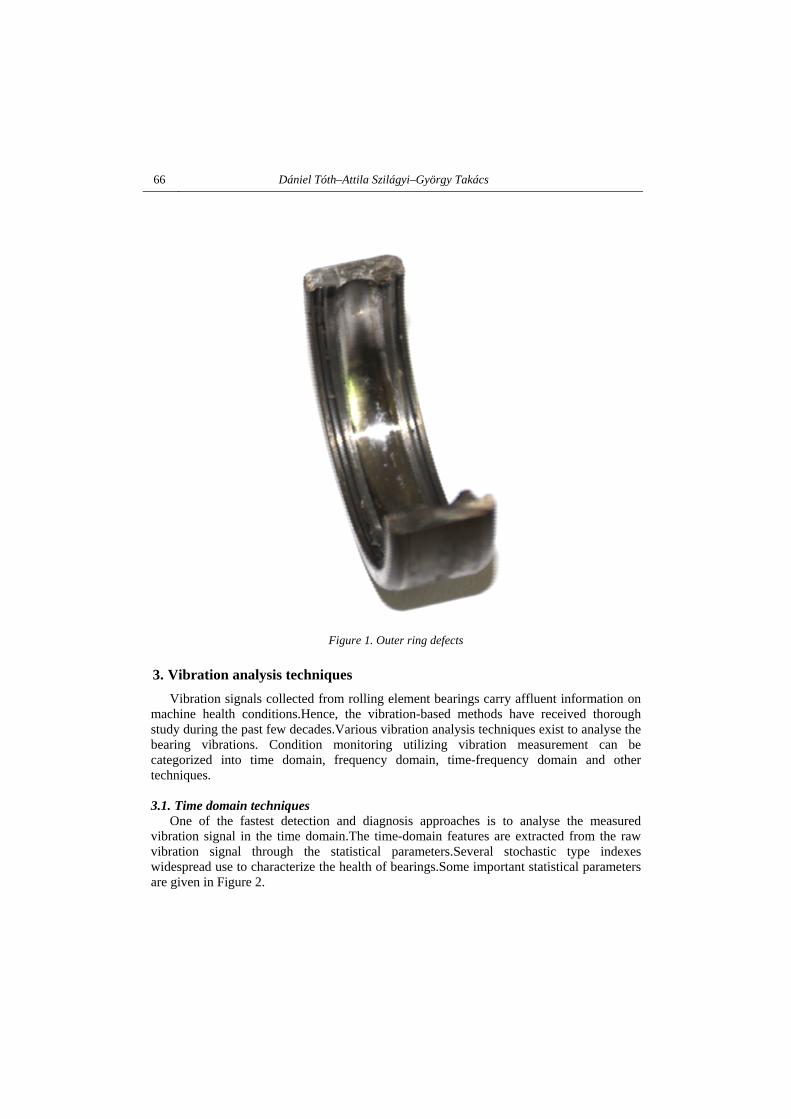
66 Dániel Tóth–Attila Szilágyi–György Takács
Figure 1. Outer ring defects
3. Vibration analysis techniques
Vibration signals collected from rolling element bearings carry affluent information on machine health conditions.Hence, the vibration-based methods have received thorough study during the past few decades.Various vibration analysis techniques exist to analyse the bearing vibrations. Condition monitoring utilizing vibration measurement can be categorized into time domain, frequency domain, time-frequency domain and other techniques.
3.1. Time domain techniques One of the fastest detection and diagnosis approaches is to analyse the measured
vibration signal in the time domain.The time-domain features are extracted from the raw vibration signal through the statistical parameters.Several stochastic type indexes widespread use to characterize the health of bearings.Some important statistical parameters are given in Figure 2.
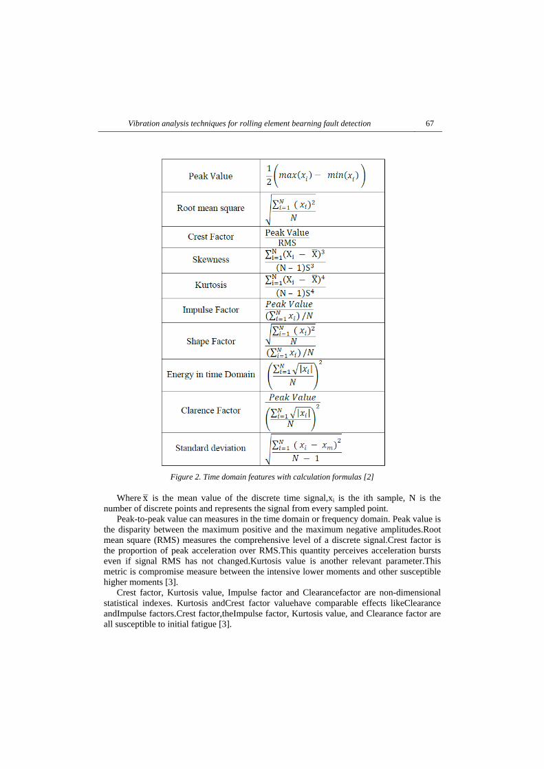
Vibration analysis techniques for rolling element bearning fault detection 67
Figure 2. Time domain features with calculation formulas [2]
Where is the mean value of the discrete time signal,xi is the ith sample, N is the number of discrete points and represents the signal from every sampled point.
Peak-to-peak value can measures in the time domain or frequency domain. Peak value is the disparity between the maximum positive and the maximum negative amplitudes.Root mean square (RMS) measures the comprehensive level of a discrete signal.Crest factor is the proportion of peak acceleration over RMS.This quantity perceives acceleration bursts even if signal RMS has not changed.Kurtosis value is another relevant parameter.This metric is compromise measure between the intensive lower moments and other susceptible higher moments [3].
Crest factor, Kurtosis value, Impulse factor and Clearancefactor are non-dimensional statistical indexes. Kurtosis andCrest factor valuehave comparable effects likeClearance andImpulse factors.Crest factor,theImpulse factor, Kurtosis value, and Clearance factor are all susceptible to initial fatigue [3].

68 Dániel Tóth–Attila Szilágyi–György Takács
3.2. Frequency domain techniques
The frequency domain analysis can reveal some information that cannot be found in time-domain.The frequency domainimplies to the analysis or display of the vibration data based on the frequency.Frequency domain techniques are the most popular approach for the interpretation of bearing failures.One principal advantage of the method is that the repetitive nature of the vibration signals is precisely displayed as peaks in the frequency spectrum at the frequency where the repetition takes place.The time domain vibration signal is typically processed into the frequency domain by the adaptation of Fourier transform, generally in the shape of fast Fourier transform (FFT) algorithm.A FFT is an algorithm to calculate the discrete Fourier transform (DFT)and its inverse.Afrequency spectrumis illustrated in Figure 3.
Figure 3. The trend of a frequency spectrum
In a frequency spectrum the horizontal axis is usually the frequency and the vertical axis is the amplitude of displacement, acceleration or velocity. The major benefit of frequencydomain techniques over time-domain techniques is that it has ability to easily ascertain the certain frequency components of interest.
3.3. Time-frequency domain techniques Several time-frequency domain techniques have been generated whichshow possibility
for detecting and diagnosing bearing problems in some of the more complicated rotating machines where the noise to signal ratio is low and a large number of frequency elements are present.
Time–frequency analysis can display the signal frequency components, identifies their time variant features.Time-frequency domain techniques have facility to handle both, non- stationary and stationary vibration signals. This is the one main advantage over frequency domain techniques.These methodsfor instancethe Wavelet transform, the short time Fourier transform and the Wigner-Ville distribution [3].
One of the most widely used time-frequency techniques is the short time Fourier transform(STFT).STFT distributes the original signal into segments with short-time window and then apply the Fourier transform to each time segment to ascertain the

Vibration analysis techniques for rolling element bearning fault detection 69
frequencies that existed in that segment. The Wavelet transform (WT) is a favoured method to diagnosis bearing faults.One advantage of WT over the STFT is that it can achieve high frequency resolutions with sharper time resolutions.
The Wigner-Ville distribution (WVD) not applies any window function so it is free from the interference between time localization and frequency resolution. Figure 4 shows the WVD in a non-stationaryoccurrence.Asterisks signalize instantaneous frequency measurements [4].
Figure 4. Wigner–Ville distribution in a non-stationary case [4]
3.4. Other Techniques Some other techniques apply to diagnosis of rolling element bearing failures for
example fuzzy logic systems, artificial neural networks (ANNs), Singular Spectrum Analysis (SSA) and so on. One advantage of ANNs that can detect bearing faults using short data length [3].
4. Conclusion
The vibration based monitoring methods are useful tools in the field of predictive maintenanceand efficacious in detecting the defects in the rolling element bearings.The present paper dealt with rolling element bearing failures and classifiedfrequent vibration analysis techniques.
5. Acknowledgement
This research was carried out as part of the TÁMOP-4.2.1.B-10/2/KONV-2010-0001 project with support by the European Union, co-financed by the European Social Fund, in the framework of the Centre of Excellence of Mechatronics and Logistics at the University of Miskolc.

70 Dániel Tóth–Attila Szilágyi–György Takács
6. References
[1] SKF, Bearing failures and their causes. Product information 401. [2] Patel, J.–Patel, V.–Patel, A.: Fault Diagnostics of Rolling Bearing based on Improve Time
and Frequency Domain Features using Artificial Neural Networks. IJSRD, Vol. 1, Issue 4, 2013.
[3] Patidar, S.–Soni, P. K.: An Overview on Vibration Analysis Techniques for the Diagnosis of Rolling Element Bearing Faults. IJETT, May 2013.
[4] Staszewski, W. J.–Robertson, A. N.: Time-frequency and time-scale analyses for structural health monitoring. DOI: 10.1098/rsta.2006, February 2007.

REVIEWING COMMITTEE
Á. DÖBRÖCZÖNI Institute of Machine- and Product Design
University of Miskolc
H-3515 Miskolc-Egyetemváros, Hungary
M. GERGELY Acceleration Bt.
K. JÁRMAI Department of Materials Handling and Logistics
University of Miskolc
H-3515 Miskolc-Egyetemváros, Hungary
I. KEREKES Institute of Mechanics
University of Miskolc,
H-3515 Miskolc-Egyetemváros, Hungary
F. J. SZABÓ Institute of Machine- and Product Design
University of Miskolc
H-3515 Miskolc-Egyetemváros, Hungary
A. SZILÁGYI Institute of Machine Tools and Mechatronics
University of Miskolc
H-3515 Miskolc-Egyetemváros, Hungary
J. PÉTER Institute of Machine and Product Design
University of Miskolc
H-3515 Miskolc-Egyetemváros, Hungary

Secreteriat of the Vice-Rector for Research and International Relations,
University of Miskolc,
Responsible for the Publication: Prof. Dr. Tamás Kékesi
Published by the Miskolc University Press under leadership of Erzsébet Burmeister
Responsible for duplication: Works manager: Erzsébet Pásztor
Editor: Dr. Ágnes Takács
Number of copies printed:
Put the Press in 2014
Number of permission: TNRT–2014–399–ME
HU ISSN 1785-6892 (PRINT); HU ISSN 2064-7522 (ONLINE)


DESIGN OF MACHINES AND
STRUCTURES Volume 4, Number 2 (2014)
PUBLICATION OF THE UNIVERSITY OF MISKOLC–
A SHORT HISTORY
The University of Miskolc (Hungary) was founded by the Empress Maria
Teresia in Selmecbánya in 1735. After the first World War the university
moved to Sopron, where in 1929, it started the series of university
publications with the title Publications of the Mining and Metallurgical
Division of the Hungarian Academy of Mining and Forestry Engineering
(Volumes I–VI). From 1934 to 1947 the Institution became the Faculty of
Mining, Metallurgical and Forestry Engineering of the József Nádor
University of Technology and Economical Sciences at Sopron. The
publications got the title Publications of the Mining and Metallurgical
Engineering Division (Volumes VII–XVI). For the last volume before 1950
– due to a further change in the name of the Institution – Technical
University, Faculties of Mining, Metallurgical and Forestry Engineering,
Publications of the Mining and Metallurgical Division was the title. For
some years after 1950 the Publications were temporarily suspended. After
the foundation of the Mechanical Engineering Faculty in Miskolc in 1949
and the movement of the Sopron Mining and Metallurgical Faculties to
Miskolc the Publications restarted with the general title Publications of the
Technical University of Heavy Industry in 1955. Four new series – Series A
(Mining), Series B (Metallurgy), Series C (Machinery) and Series D
(Natural Sciences) – were founded in 1976. These came out both in foreign
languages (English, German and Russian) and in Hungarian. In 1990, right
after the foundation of some new faculties, the university was renamed to
University of Miskolc. At the same time the structure of the Publications
was reorganized so that it could follow the faculty structure. Accordingly
three new series were established: Series E (Legal Sciences), Series F
(Economical Sciences) and Series G (Humanities and Social Sciences). The
latest series, the Series H (European Integration Studies) was founded in
2002. Design of Machines and Structures (HU ISSN 1785-6892 [Print],
HU ISSN 2064-7522 [Online]) first published in 2003 as a part of the
Series C.


![Arya, Suresh - Design of Structures and Foundations for Vibrating Machines [1984].pdf](https://img.pdfslide.net/doc/110x75/55cf9d1d550346d033ac4dce/arya-suresh-design-of-structures-and-foundations-for-vibrating-machines.jpg)