Embed Size (px)
Citation preview

HU ISSN 1785-6892 in print
HU ISSN 2064-7522 online
DESIGN OF MACHINES AND STRUCTURES
A Publication of the University of Miskolc
Volume 10, Number 1
Miskolc University Press
2020

EDITORIAL BOARD
Á. DÖBRÖCZÖNI Institute of Machine and Product Design
Editor in Chief University of Miskolc
H-3515 Miskolc-Egyetemváros, Hungary
Á. TAKÁCS Institute of Machine and Product Design
Assistant Editor University of Miskolc
H-3515 Miskolc-Egyetemváros, Hungary
R. CERMAK Department of Machine Design
University of West Bohemia
Univerzitní 8, 30614 Plzen, Czech Republic
B. M. SHCHOKIN Consultant at Magna International Toronto
W. EICHLSEDER Institut für Allgemeinen Maschinenbau
Montanuniversität Leoben,
Franz-Josef Str. 18, 8700 Leoben, Österreich
S. VAJNA Institut für Maschinenkonstruktion,
Otto-von-Guericke-Universität Magdeburg,
Universität Platz 2, 39106 Magdeburg, Deutschland
P. HORÁK Department of Machine and Product Design
Budapest University of Technology and Economics
H-1111 Budapest, Műegyetem rkp. 9.
MG. ép. I. em. 5.
K. JÁRMAI Institute of Materials Handling and Logistics
University of Miskolc
H-3515 Miskolc-Egyetemváros, Hungary
L. KAMONDI Institute of Machine and Product Design
University of Miskolc
H-3515 Miskolc-Egyetemváros, Hungary
GY. PATKÓ Department of Machine Tools
University of Miskolc
H-3515 Miskolc-Egyetemváros, Hungary
J. PÉTER Institute of Machine and Product Design
University of Miskolc
H-3515 Miskolc-Egyetemváros, Hungary
CONTENTS
Alhafadhi, Mahmood–Krállics, György:
Effect of the welding parameters on residual stresses in pipe weld using numerical
simulation ............................................................................................................................... 5
Ficzere, Péter–Lukács, Norbert László:
The possibilities of intelligent manufacturing methods ....................................................... 13
Kapitány, Pálma–Lénárt, József:
Control of a cable robot on PSOC cypress platform ............................................................ 20
Mobark, Haidar–Lukács, János:
Mismatch effect on fatigue crack propagation limit curves of GMAW joints made
of S960QL and S960TM type base materials ....................................................................... 28
Rónai, László:
Development of an electric measurement system for rapid determination
of the friction coefficient ...................................................................................................... 39
Szabó, J. Ferenc:
Evolutionary based system for qualification and evaluation – A case study ........................ 49

Design of Machines and Structures, Vol. 10, No. 1 (2020), pp. 5–12.
Doi: 10.32972/dms.2020.001
EFFECT OF THE WELDING PARAMETERS ON RESIDUAL STRESSES
IN PIPE WELD USING NUMERICAL SIMULATION
MAHMOOD ALHAFADHI1–GYÖRGY KRÁLLICS2
University of Miskolc, Faculty of Material Science and Engineering,
3515, Miskolc-Egyetemváros
Abstract: The objective of this article is to predict the residual welding stress in a dissimilar
pipe weld. The 2D model, instead of 3D was used to reduce the time and cost of the numerical
calculation. The 2D numerical simulation MSC MARC code is used to predict the residual
stress developed during pipe welding. The present model was validated using hardness
measurement. Good agreement was found between the measurement and numerical
simulation results. The effects of welding parameters on residual stress field on the outer and
inner surface were assessed. The effect of welding parameter (welding current) is examined.
The axial and hoop residual stresses in dissimilar pipe joints of different thickness for pipe
weld were simulated in outer and inner surfaces. When the other parameters remain fixed,
and the current has great effect on the weld shape and size, and then affects the residual stress
level significantly.
Keywords: Numerical Simulation, Welding Pipe, Residual stress.
1. INTRODUCTION
Welding is a reliable and efficient metal joining process between two parts of
dissimilar pipes. Arc welding joints are more extensively used in the fabrication
industry, oil and gas pipeline, offshore structures, and pressure vessels. Welding
residual stresses are caused by differential thermal expansion and contraction of the
weld metal and dissimilar base metal. Further, these residual stresses can be of either
tensile type or the compressive type, depending upon the location of the non-uniform
volumetric change. Numerical simulation is used to predict residual stresses due to
the complexity of the shape structure. Nowadays, it is possible to use numerical
simulation techniques to predict the residual stresses in welded structures and it can
be employed to simulate welding temperature field and welding deformation. [1–7].
In order to reduce the computational time and cost, most of the researchers choose
the 2D model. Brickstad and Josefon [8] employed 2D model to simulate welding of
stainless steel pipe in thermo-mechanical finite element analysis. Dean Deng et al.
[9] presented a 2D FE model for simulating residual stresses during multipass
welding of a pipe. The distribution of residual stress in welded pipe structures
depends on several factors such as structural dimensions material properties, and
heat input, etc. Siddique M. et al. [10] analysed the residual stress fields in circum-
6 Mahmood Alhafadhi–György Krállics
ferentially arc welded and studied the effect of two basic welding parameters
including welding current and speed. However, there are minimal studies on effects
of welding parameters on residual stresses in dissimilar welded pipe joints. In this
study, the prediction of residual stresses in a dissimilar pipe weld joint made of
E355K2 and P460NH_1 is studied by using 2D finite element method. This study
also presents the 2D FE model of pipe joint to investigate the effect of welding
current on residual stress distribution.
2. 2D AND 3D MODELLING PROCESS
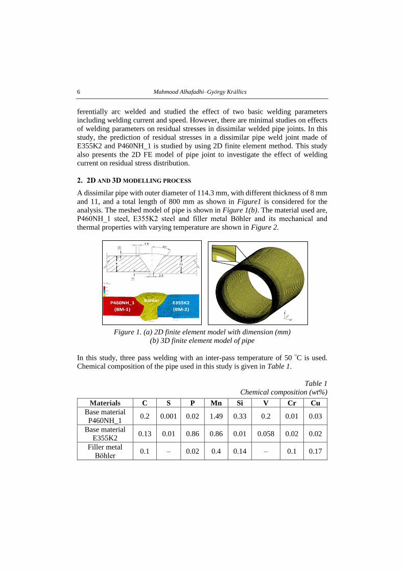
A dissimilar pipe with outer diameter of 114.3 mm, with different thickness of 8 mm
and 11, and a total length of 800 mm as shown in Figure1 is considered for the
analysis. The meshed model of pipe is shown in Figure 1(b). The material used are,
P460NH_1 steel, E355K2 steel and filler metal Böhler and its mechanical and
thermal properties with varying temperature are shown in Figure 2.
Figure 1. (a) 2D finite element model with dimension (mm)
(b) 3D finite element model of pipe
In this study, three pass welding with an inter-pass temperature of 50 ᴼC is used.
Chemical composition of the pipe used in this study is given in Table 1.
Table 1
Chemical composition (wt%)
Materials C S P Mn Si V Cr Cu
Base material
P460NH_1 0.2 0.001 0.02 1.49 0.33 0.2 0.01 0.03
Base material
E355K2 0.13 0.01 0.86 0.86 0.01 0.058 0.02 0.02
Filler metal
Böhler 0.1 – 0.02 0.4 0.14 – 0.1 0.17
Effect of the welding parameters on residual stresses in pipe weld using numerical simulation 7
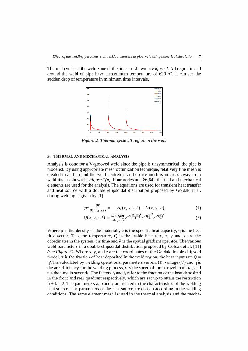
Thermal cycles at the weld zone of the pipe are shown in Figure 2. All region in and
around the weld of pipe have a maximum temperature of 620 oC. It can see the
sudden drop of temperature in minimum time intervals.
Figure 2. Thermal cycle all region in the weld
3. THERMAL AND MECHANICAL ANALYSIS
Analysis is done for a V-grooved weld since the pipe is unsymmetrical, the pipe is
modeled. By using appropriate mesh optimization technique, relatively fine mesh is
created in and around the weld centreline and coarse mesh is in areas away from
weld line as shown in Figure 1(a). Four nodes and 86,642 thermal and mechanical
elements are used for the analysis. The equations are used for transient heat transfer
and heat source with a double ellipsoidal distribution proposed by Goldak et al.
during welding is given by [1]
𝑝𝑐𝜕𝑇
𝜕𝑡(𝑥,𝑦,𝑧,𝑡)= −𝛻𝑞(𝑥, 𝑦, 𝑧, 𝑡) + 𝑄(𝑥, 𝑦, 𝑧,) (1)
𝑄(𝑥, 𝑦, 𝑧, 𝑡) = 𝟔√𝟑 𝒇𝒊𝜼𝑰𝑽
𝒂𝒃𝒄𝒇𝝅√𝝅𝒆
−𝟑(𝒙−𝒗𝒕
𝒂)
𝟐
𝒆−𝟑(
𝒚𝒃
)𝟐
𝒆−𝟑(
𝒛𝒄
)𝟐
(2)
Where p is the density of the materials, c is the specific heat capacity, q is the heat
flux vector, T is the temperature, Q is the inside heat rate, x, y and z are the
coordinates in the system, t is time and ∇ is the spatial gradient operator. The various
weld parameters in a double ellipsoidal distribution proposed by Goldak et al. [11]
(see Figure 3). Where x, y, and z are the coordinates of the Goldak double ellipsoid
model, π is the fraction of heat deposited in the weld region, the heat input rate Q =
ηVI is calculated by welding operational parameters current (I), voltage (V) and η is
the arc efficiency for the welding process, v is the speed of torch travel in mm/s, and
t is the time in seconds. The factors ff and fr refer to the fraction of the heat deposited
in the front and rear quadrant respectively, which are set up to attain the restriction
ff + fr = 2. The parameters a, b and c are related to the characteristics of the welding
heat source. The parameters of the heat source are chosen according to the welding
conditions. The same element mesh is used in the thermal analysis and the mecha-
8 Mahmood Alhafadhi–György Krállics
nical analysis. During the welding process, the solid-state phase transfor-mation
occurs in the base metal and the weld metal. Therefore the total strain rate can be
expressed as follows:
𝛆 = 𝛆𝒆 + 𝜺𝒑 + 𝜺𝒕𝒉 (3)
Where the elastic strain is 𝜺𝒆, the plastic strain 𝜺𝒑 and 𝜺𝒕𝒉 is the thermal strain.
Figure 3. Double-ellipsoidal volumetric heat source model
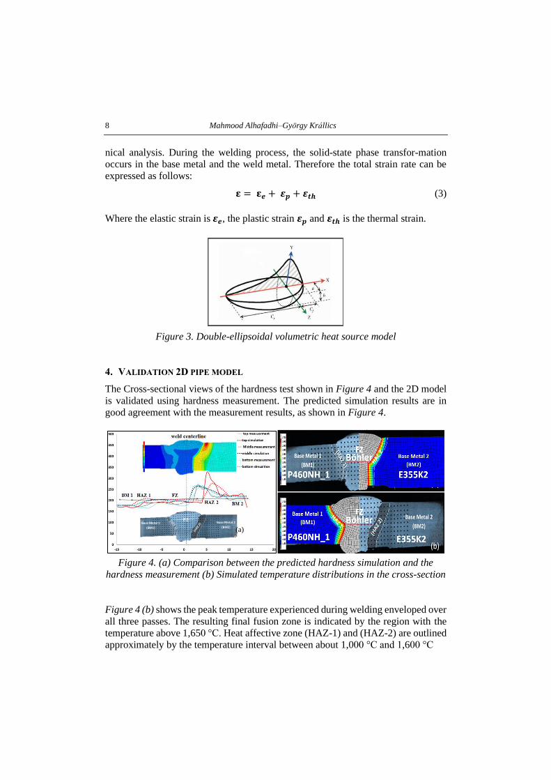
4. VALIDATION 2D PIPE MODEL
The Cross-sectional views of the hardness test shown in Figure 4 and the 2D model
is validated using hardness measurement. The predicted simulation results are in
good agreement with the measurement results, as shown in Figure 4.
Figure 4. (a) Comparison between the predicted hardness simulation and the
hardness measurement (b) Simulated temperature distributions in the cross-section
Figure 4 (b) shows the peak temperature experienced during welding enveloped over
all three passes. The resulting final fusion zone is indicated by the region with the
temperature above 1,650 °C. Heat affective zone (HAZ-1) and (HAZ-2) are outlined
approximately by the temperature interval between about 1,000 °C and 1,600 °C
(a)
Effect of the welding parameters on residual stresses in pipe weld using numerical simulation 9
5. RESULTS AND DISCUSSION
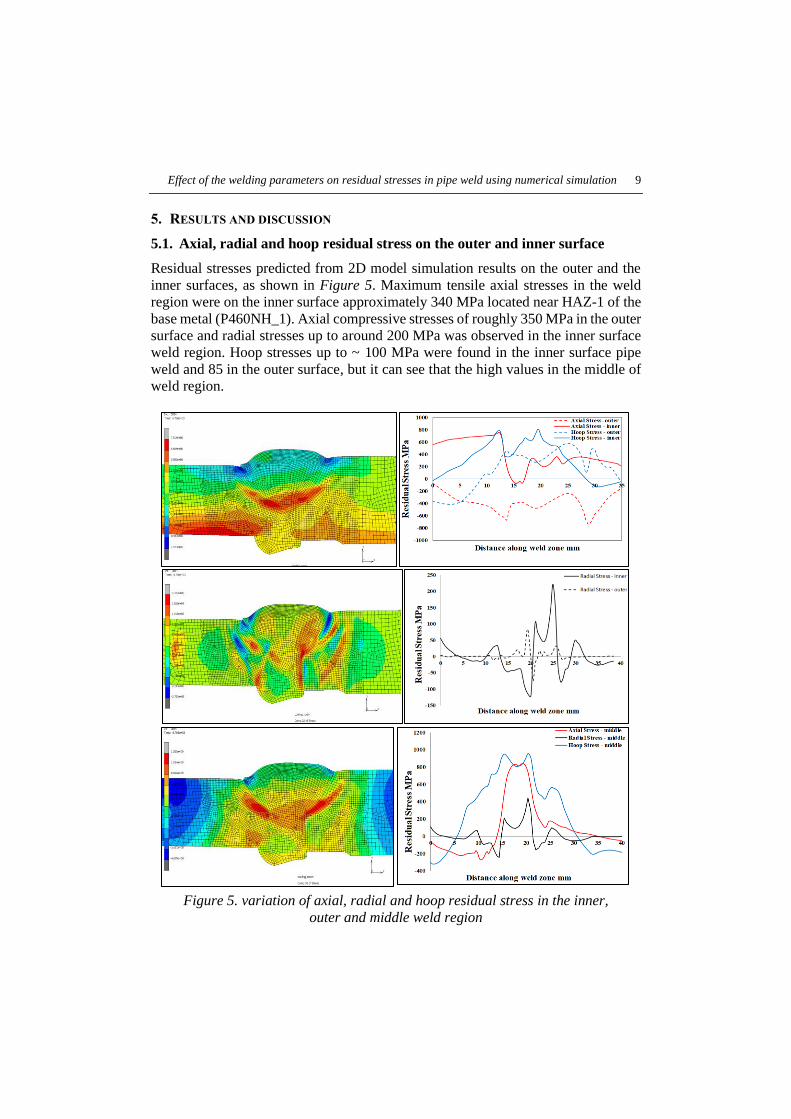
5.1. Axial, radial and hoop residual stress on the outer and inner surface
Residual stresses predicted from 2D model simulation results on the outer and the
inner surfaces, as shown in Figure 5. Maximum tensile axial stresses in the weld
region were on the inner surface approximately 340 MPa located near HAZ-1 of the
base metal (P460NH_1). Axial compressive stresses of roughly 350 MPa in the outer
surface and radial stresses up to around 200 MPa was observed in the inner surface
weld region. Hoop stresses up to ~ 100 MPa were found in the inner surface pipe
weld and 85 in the outer surface, but it can see that the high values in the middle of
weld region.
Figure 5. variation of axial, radial and hoop residual stress in the inner,
outer and middle weld region
10 Mahmood Alhafadhi–György Krállics
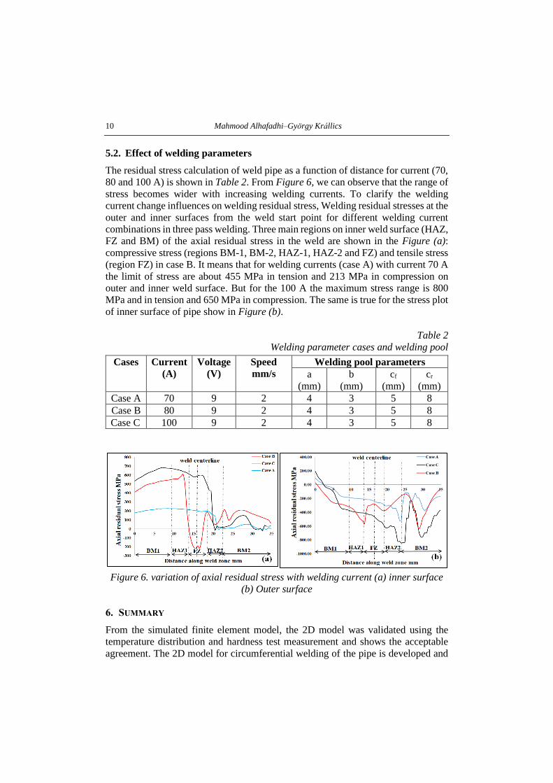
5.2. Effect of welding parameters
The residual stress calculation of weld pipe as a function of distance for current (70,
80 and 100 A) is shown in Table 2. From Figure 6, we can observe that the range of
stress becomes wider with increasing welding currents. To clarify the welding
current change influences on welding residual stress, Welding residual stresses at the
outer and inner surfaces from the weld start point for different welding current
combinations in three pass welding. Three main regions on inner weld surface (HAZ,
FZ and BM) of the axial residual stress in the weld are shown in the Figure (a):
compressive stress (regions BM-1, BM-2, HAZ-1, HAZ-2 and FZ) and tensile stress
(region FZ) in case B. It means that for welding currents (case A) with current 70 A
the limit of stress are about 455 MPa in tension and 213 MPa in compression on
outer and inner weld surface. But for the 100 A the maximum stress range is 800
MPa and in tension and 650 MPa in compression. The same is true for the stress plot
of inner surface of pipe show in Figure (b).
Table 2
Welding parameter cases and welding pool
Cases Current
(A)
Voltage
(V)
Speed
mm/s
Welding pool parameters
a
(mm)
b
(mm)
cf
(mm)
cr
(mm)
Case A 70 9 2 4 3 5 8
Case B 80 9 2 4 3 5 8
Case C 100 9 2 4 3 5 8
Figure 6. variation of axial residual stress with welding current (a) inner surface
(b) Outer surface
6. SUMMARY
From the simulated finite element model, the 2D model was validated using the
temperature distribution and hardness test measurement and shows the acceptable
agreement. The 2D model for circumferential welding of the pipe is developed and
Effect of the welding parameters on residual stresses in pipe weld using numerical simulation 11
the residual stresses for outer and inner surfaces are predicted. Axial residual stress
changes from tensile to compressive from inner to the outer surface after the welding
and the high value found in near and around (HAZ-2) for base metal (P460NH_1).
Hoop residual stress changes from tensile to compressive in the outer surface and the
high value found in near and around (FZ). The magnitude of residual stress
distribution became wider when welding current increases.
REFERENCES
[1] Mobark, H., Lukács, J. (2018). HCF design curves for high strength steel
welded joints. Design of Machines and Structures, Vol. 8, No. 2, pp. 39–51.
[2] Alhafadhi, Mahmood H., Krallics, György (2019). Numerical simulation
prediction and validation two dimensional model weld pipe. Machines.
Technologies. Materials. Vol. 13, No. 10, pp. 447–450.
[3] Szávai, Sz., Bézi, Z., Rózsahegyi, P. (2016). Material Characterization and
Numerical Simulation of a Dissimilar Metal Weld. Procedia Structural
Integrity, Vol. 2, pp. 1023–1030.
[4] Szávai, Sz., Bézi, Z., Ohms, C. (2016). Numerical simulation of dissimilar
metal welding and its verification for determination of residual stresses.
Frattura ed Integrita Strutturale, Vol. 10, No. 36, pp. 36–45.
[5] Alhafadhi, Mahmood Hasan, Krallics, György (2019). The effect of heat
input parameters on residual stress distribution by numerical simulation,
iop conference series. Materials Science and Engineering, Vol. 613. No. 1.
p. 012035.
[6] Vemanaboina, Harinadh, Akella, Suresh, Buddu, Ramesh Kumar (2014).
Welding process simulation model for temperature and residual stress
analysis. Procedia materials science, Vol. 6, pp. 1539–1546.
[7] Ghosh, P. K., Ghosh, Aritra K. (2004). Control of residual stresses affecting
fatigue life of pulsed current gas-metal-arc weld of high-strength aluminum
alloy. Metallurgical and materials transactions, Vol. 35, No. 8, pp. 2439–
2444.
[8] Brickstad, B., Josefson, B. L. (1998). A parametric study of residual stresses in
multi-pass butt-welded stainless steel pipes. International journal of pressure
vessels and piping, Vol. 75, pp. 11–25.
[9] Deng, Dean, Hidekazu Murakawa, Wei Liang (2008). Numerical and
experimental investigations on welding residual stress in multi-pass butt-
welded austenitic stainless steel pipe. Computational Materials Science, Vol.
42, No. 2, pp. 234–244.

12 Mahmood Alhafadhi–György Krállics
[10] Siddique, M., Abid, M., Junejo, H. F., Mufti, R. A. (2005). 3-D finite element
simulation of welding residual stresses in pipe-flange joints: effect of welding
parameters. In materials science forum, Vol. 490, pp. 79–84.
[11] Goldak, John, Aditya Chakravarti, Bibby, Malcolm (1984). A new finite
element model for welding heat sources. Metallurgical transactions, Vol. 15,
No. 2, pp. 299–305.
Design of Machines and Structures, Vol. 10, No. 1 (2020), pp. 13–19.
Doi: 10.32972/dms.2020.002
THE POSSIBILITIES OF INTELLIGENT MANUFACTURING METHODS
PÉTER FICZERE–NORBERT LÁSZLÓ LUKÁCS
Budapest University of Technology and Economics,
Department of Vehicle Elements and Vehicle-Structure Analysis
1111 Budapest, Stoczek u. 2.
Abstract: Additive production technologies made the realization of individually designed,
highly complicated geometric structures in practically all fields of industry and human ther-
apy (implantation) possible. In order to minimalize the risk of failure originating from pro-
duction technology the continuous development of measurements technologies provides the
possibility to track the parameters of production and if necessary to ensure their modification.
The great number of recorded production data (big data) at the same time can be used in the
quality control of the product.
Keywords: Additive manufacturing, methodology, IoT, i4.0, Remote control for manu-facturers
1. INTRODUCTION
Nowadays we can hear that we have been living in the fourth industrial revolution.
The first industrial revolution was the transition of new manufacturing methods, the
transition from hand production to machines, the second was the time of the mass
production and the third was time of automation [1]. In case of fourth industrial rev-
olution more technical feature can be highlighted.
Tracking of individual products, monitoring and analysing process of manufac-
turing conditions and autonomous failure detection can be possible with machine
monitoring systems with high quality sensors (for example RFID systems or differ-
ent measuring systems) and smart industry networks. With assistance of these tools
and devices the synergy between smart production lines and information technolo-
gies can be put in practice. It means the collection, storing and dispersing of high
complexity data which can be set in industrial service by intelligent analysing soft-
ware. The high volume of data can provide multivarious analysis for different aspects
of production [2].
The industrial measuring and data collecting methods have numerous advantages.
Places of failures can be predicted and these methods have a significant role in qual-
ity assurance (QA). Tracking of products life cycle is a highly recommend task dur-
ing the production and logistical process. Full transparency in material flow, tracking
of production can provide great traceability. With evidence record and store of pro-
duction data, the identification and certification of individual product can remain
14 Péter Ficzere–Norbert László Lukács
after the delivery. Quality assurance and magisterial tests can be done more econom-
ically and quicker [2].
Analysis of data can highly support the sufficient maintenance process and the
quick intervention either. The real time online data collection and autonomous fail-
ure detection can help the precise manufacturing. For these reasons the amount of
waste product can be highly reduced. Continuous data collection can help the verifi-
cation of certifications.
In the last few years, futurologists and scientist who are involved in the education
of design have been studied that which parts of the industry can achieve break-
throughs in the next few years and can affect to everyday life: AI (artificial intelli-
gence), autonomous cars and autonomous manufacturing were predicted as the fifth
industrial revolution [3], [4], [5]. Participants of the sixth industrial revolution may
can be cyborgs, which means the cooperation of cybernetic and organic beings. In
this case we can speak about the hybrids of bits, atoms, gene and nanotechnology.
2. THE POSSIBILITIES OF ADDITIVE MANUFACTURING
Remarkable part of Industry 4.0 is the IoT (Internet of Things) where the equipment
is connected in common networks and these instruments can communicate to each
other, the big data, where all of data are collected and a more complex analysis is
possible with them [6]. Big data can help to time maintenances and some failure can
be predicted. The human-machine connection (cobots) come into prominence with
the Industry 4.0. Additive manufacturing technologies also must be mentioned,
which manufacturing technologies can provide nearly infinite possibilities and pro-
duce complex parts in an economical way. [7], [8].
2.1. Additive manufacturing with AI
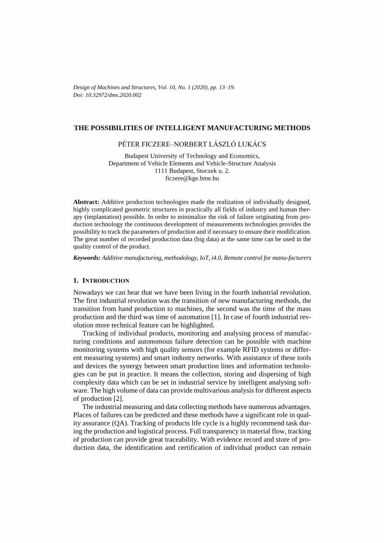
The newest 3D printers are not bounded to a frame. It means that these machines can
change their position, therefore there are no limits with size. These experimental
machines can preannounce how will the future look like.
Figure 1. 3D printer spider [9]
The possibilities of intelligent manufacturing methods 15
In the first picture there is an autonomous 3D printer which operates with the help
of artificial intelligence (AI). Every single leg has a 3D printer head and these legs
can communicate to each other. These “heads” can solve individual problems and
this method is optimised by the communication of them. The sensors in legs can help
them to avoid hazards and they also can inform other machines about them. The
cooperation of these printers can create functioning products. They can control their
own energy consumption and charge themselves if it is needed.
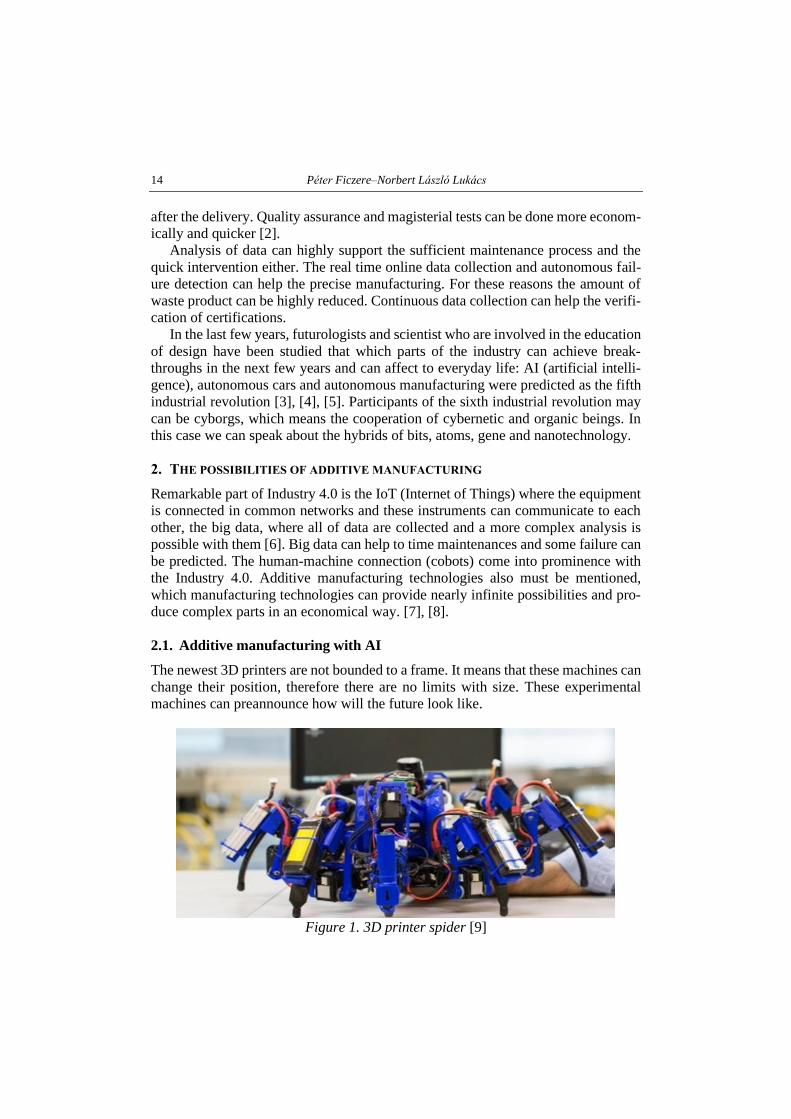
Modern software can optimise the 3D printers and at the same time these systems
can pay attention to mechanical properties, accuracy and aesthetics [10]. Figure 2
shows the influence of adaptive layer height. This function can reduce layer height
where it is needed, for example where rounded or complex shaped areas are and
allow higher layers for the quicker manufacturing where the resolution is not im-
portant.
Figure 2. Adaptive layer height [11]
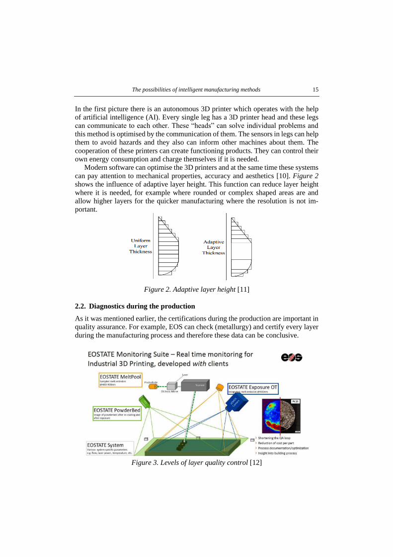
2.2. Diagnostics during the production
As it was mentioned earlier, the certifications during the production are important in
quality assurance. For example, EOS can check (metallurgy) and certify every layer
during the manufacturing process and therefore these data can be conclusive.
Figure 3. Levels of layer quality control [12]
16 Péter Ficzere–Norbert László Lukács
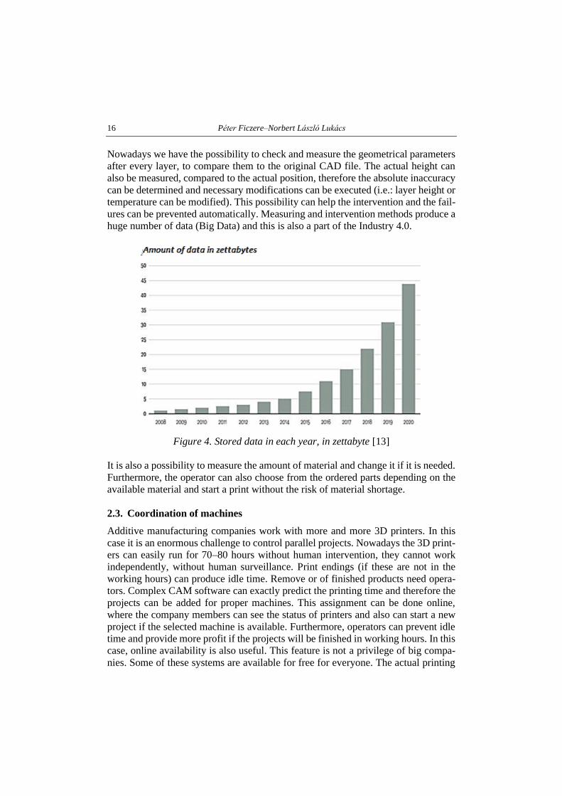
Nowadays we have the possibility to check and measure the geometrical parameters
after every layer, to compare them to the original CAD file. The actual height can
also be measured, compared to the actual position, therefore the absolute inaccuracy
can be determined and necessary modifications can be executed (i.e.: layer height or
temperature can be modified). This possibility can help the intervention and the fail-
ures can be prevented automatically. Measuring and intervention methods produce a
huge number of data (Big Data) and this is also a part of the Industry 4.0.
Figure 4. Stored data in each year, in zettabyte [13]
It is also a possibility to measure the amount of material and change it if it is needed.
Furthermore, the operator can also choose from the ordered parts depending on the
available material and start a print without the risk of material shortage.
2.3. Coordination of machines
Additive manufacturing companies work with more and more 3D printers. In this
case it is an enormous challenge to control parallel projects. Nowadays the 3D print-
ers can easily run for 70–80 hours without human intervention, they cannot work
independently, without human surveillance. Print endings (if these are not in the
working hours) can produce idle time. Remove or of finished products need opera-
tors. Complex CAM software can exactly predict the printing time and therefore the
projects can be added for proper machines. This assignment can be done online,
where the company members can see the status of printers and also can start a new
project if the selected machine is available. Furthermore, operators can prevent idle
time and provide more profit if the projects will be finished in working hours. In this
case, online availability is also useful. This feature is not a privilege of big compa-
nies. Some of these systems are available for free for everyone. The actual printing
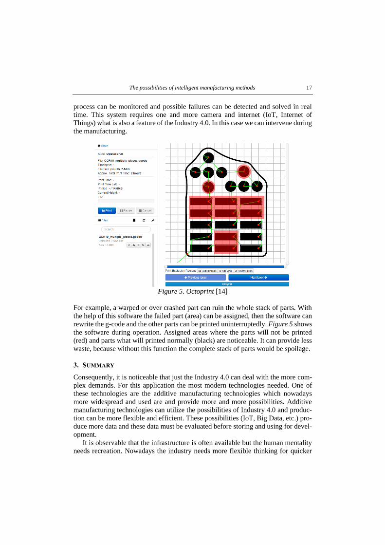
The possibilities of intelligent manufacturing methods 17
process can be monitored and possible failures can be detected and solved in real
time. This system requires one and more camera and internet (IoT, Internet of
Things) what is also a feature of the Industry 4.0. In this case we can intervene during
the manufacturing.
Figure 5. Octoprint [14]
For example, a warped or over crashed part can ruin the whole stack of parts. With
the help of this software the failed part (area) can be assigned, then the software can
rewrite the g-code and the other parts can be printed uninterruptedly. Figure 5 shows
the software during operation. Assigned areas where the parts will not be printed
(red) and parts what will printed normally (black) are noticeable. It can provide less
waste, because without this function the complete stack of parts would be spoilage.
3. SUMMARY
Consequently, it is noticeable that just the Industry 4.0 can deal with the more com-
plex demands. For this application the most modern technologies needed. One of
these technologies are the additive manufacturing technologies which nowadays
more widespread and used are and provide more and more possibilities. Additive
manufacturing technologies can utilize the possibilities of Industry 4.0 and produc-
tion can be more flexible and efficient. These possibilities (IoT, Big Data, etc.) pro-
duce more data and these data must be evaluated before storing and using for devel-
opment.
It is observable that the infrastructure is often available but the human mentality
needs recreation. Nowadays the industry needs more flexible thinking for quicker
18 Péter Ficzere–Norbert László Lukács
and economical reactions for challenges of Industry and Economy. It means the use
of acquired knowledge is not enough but continuous renewal and development is
needed not just for the machine side but for the human side either.
REFERENCES
[1] Ficzere P., Borbás L. (2019). Az ipar 4.0 hatása az egyénre szabható implan-
táció tervezési folyamatára. IV. Gépészeti Szakmakultúra Konferencia, Buda-
pest, Gépipari Tudományos Egyesület, p4, ISBN 978-963-9058-41-5.
[2] http://www.industry4.hu (letöltve 2019. 11. 13.)
[3] Szabó I., Török Á. (2018). Autonóm közforgalmú közösségi közúti gép-
járművek társadalmi elfogadtatásának vizsgálata. In: Péter, Tamás (szerk.)
IFFK 2018: XII. Innováció és fenntartható felszíni közlekedés. Budapest,
Magyar Mérnökakadémia (MMA), pp. 333–336, ISBN 978-963-88875-3-5.
[4] Pauer, G., Török, Á. (2019). Static system optimum of linear traffic distribu-
tion problem assuming an intelligent and autonomous transportation system.
Periodica Polytechnica Transportation Engineering, 47 (1), pp. 64–67.
[5] Török, Á., Szalay, Z., Uti, G., Verebélyi, B. (2020). Modelling the effects of
certain cyber-attack methods on urban autonomous transport systems, case
study of Budapest. Journal of Ambient Intelligence and Humanized Compu-
ting, 11, pp. 1629–1643, https://doi.org/10.1007/s12652-019-01264-8.
[6] Lekić, M., Rogić, K., Boldizsár, A., Zöldy, M., Török, Á. (2019). Big Data in
logistics. Periodica Polytechnica Transportation Engineeringm, https://doi.
org/10.3311/PPtr.14589.
[7] Ficzere, P., Borbás, L., Török, Á. (2013). Economical investigation of rapid
prototyping. International Journal for Traffic and Transport Engineering, 3
(3), pp. 344–350, doi: https://doi.org/10.7708/ijtte.2013.3(3).09.
[8] Ficzere P. (2019). Alkatrészek munkatérben történő elhelyezésének a gyártási
költségekre gyakorlolt hatása additív gyártástechnológiák esetén. GÉP, LXX.
évf., 2019/3., pp 26–29.
[9] Livio Dalloro, (head of research group, siemens corporation, corporate tech-
nology), Milánó, Italy (2014), https://www.21stcentech.com/spider-robots-
bring-portability-autonomy-3d-printing/.
[10] Győri, M., Ficzere, P. (2017). Use of Sections in the Engineering Practice.
Periodica Polytechnica Transportation Engineering, 45 (1), pp. 21–24, doi:
https://doi.org/10.3311/PPtr.9144.
[11] Broek, Johan J., Horváth, Imre, de Smit, Bram, Lennings, Alex F., Vergeest,
Joris S.M. (1998). A Survey of the State of Art in Thick Layered Manufacturing

The possibilities of intelligent manufacturing methods 19
of Large Objects and the Presentation of a Newly Developed System. Univer-
sity of Texas at Austin.
[12] Falk Gy. (2019). Az asztali és az ipari fémnyomtatás közötti különbségek.
Előadás. Ipar Napjai – Mach-Tech, Budapest, 2019. május 16.
[13] What is Hadoop? https://www.sas.com/en_us/insights/big-data/hadoop.html
(letöltve: 2019. 12. 17.).
[14] https://plugins.octoprint.org/plugins/excluderegion (letöltve: 2020. 02. 15.).
Design of Machines and Structures, Vol. 10, No. 1 (2020), pp. 20–27.
Doi: 10.32972/dms.2020.003
CONTROL OF A CABLE ROBOT ON PSOC CYPRESS PLATFORM
PÁLMA KAPITÁNY1–JÓZSEF LÉNÁRT2
1 Robert Bosch Department of Mechatronics,
Faculty of Mechanical Engineering and Informatics
University of Miskolc, Egyetemváros, H-3515 Miskolc, Hungary,
e-mail: [email protected] 2 Robert Bosch Department of Mechatronics,
Faculty of Mechanical Engineering and Informatics
University of Miskolc, Egyetemváros , H-3515 Miskolc, Hungary,
e-mail: [email protected]
Abstract: This paper deals with the control of a cable model robot. The continuous motion
of the end effector is provided by velocity control of four DC motors. In each uniform time
step the rotational speed of the motors are predicted based on the assumption of constant path
velocity of the end effector in order to move it to prescribed position. In the next time step
the rotational speed of the motors are calculated from the difference between the actual po-
sition and the target one. This way the discrepancy between the actual position and the pre-
scribed one is corrected step-by-step. The control algorithm is implemented on Cypress Sem-
iconductor CY8CKIT PSoC 5LP microcontroller.
Keywords: Cable robot, Velocity control of DC motors, Microcontroller, Inverse kinematics
1. INTRODUCTION
Cable robots are frequently used e.g. to move cameras in sport halls and stadiums
and for logistics in high stores [1]. Big working space and fast positioning are the
advantages of cable robots. There are two main groups of cable robots planar ([5],
[6]), and spatial ones ([7], [8]).
The most important purpose of the plane movers is the precise positioning, it is
utilized in cable drawing machines, in industrial applications they carry out logistical
tasks, or external cleaning of office buildings. 3D cable robots are capable of not
only positioning, but can also control the orientation of the end-effector being
moved. Robots are popular in the airplane industry, because they can follow compli-
cated spatial shape when welding wing elements, similarly to painting.
Nowadays it is also used for nonindustrial purposes, e.g., flight simulation, theatri-
cal performances, solar panel assembly, and health rehabilitation exercises, etc. [1].
Corresponding Author

Control of a cable robot on PSoC Cypress platform 21
In a previous article [2], the authors of this paper published a test bench that ap-
proximated a curve path by a polygon. Four DC motors were controlled with one
master and four slave microcontrollers. The motion of the end-effector was non-
continuous, because the master waited for the slaves to finish their tasks in each
increment, i.e., to perform the motion along one polygon side.
This robot has been upgraded, with the complete replacement of the control unit
by a single Cypress Semiconductor CY8CKIT PSoC 5LP microcontroller. As a re-
sult of the current research it has a continuous speed control. It is checking the pre-
dicted progress at each time step. When the length of the cables are lagging behind
the calculated values the speed of the motors are increased, and vice versa.
The organization of this paper is as follows. In Section 2, the inverse kinematics
of the robot is discussed. In Section 3, the control of the four motors are described.
Finally, summary is given in Section 4.
2. INVERSE KINEMATICS
Figure 1 shows the picture of a planar cable robot. The end effector is suspended by
four cables, which are winded on winches. The winches are driven by four DC mo-
tors identified by letters a, b, c, d. The displacement increment of the end effector is
sketched in Figure 2. The end-effector of cable robot denoted by blue disc is moved
in plane xy.
Figure 1. Planar cable robot
22 Pálma Kapitány–József Lénárt
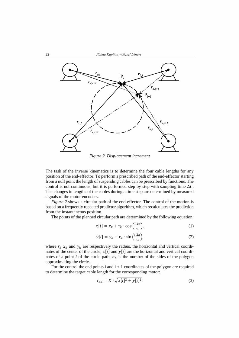
Figure 2. Displacement increment
The task of the inverse kinematics is to determine the four cable lengths for any
position of the end-effector. To perform a prescribed path of the end-effector starting
from a null point the length of suspending cables can be prescribed by functions. The
control is not continuous, but it is performed step by step with sampling time ∆𝑡 . The changes in lengths of the cables during a time step are determined by measured
signals of the motor encoders.
Figure 2 shows a circular path of the end-effector. The control of the motion is
based on a frequently repeated predictor algorithm, which recalculates the prediction
from the instantaneous position.
The points of the planned circular path are determined by the following equation:
𝑥[𝑖] = 𝑥𝑘 + 𝑟𝑘 ∙ cos (𝑖∙2𝜋
𝑛𝑜), (1)
𝑦[𝑖] = 𝑦𝑘 + 𝑟𝑘 ∙ sin (𝑖∙2𝜋
𝑛𝑜), (2)
where 𝑟𝑘 𝑥𝑘 and 𝑦𝑘 are respectively the radius, the horizontal and vertical coordi-
nates of the center of the circle, 𝑥[𝑖] and 𝑦[𝑖] are the horizontal and vertical coordi-
nates of a point 𝑖 of the circle path, 𝑛𝑜 is the number of the sides of the polygon
approximating the circle.
For the control the end points i and i + 1 coordinates of the polygon are required
to determine the target cable length for the corresponding motor:
𝑟𝑎,𝑖 = 𝐾 ∙ √𝑥[𝑖]2 + 𝑦[𝑖]2, (3)
Control of a cable robot on PSoC Cypress platform 23
𝑟𝑏,𝑖 = 𝐾 ∙ √(𝑥[𝑖] − ℎ)2 + 𝑦[𝑖]2, (4)
𝑟𝑐,𝑖 = 𝐾 ∙ √𝑥[𝑖]2 + (𝑦[𝑖] + 𝑣)2, (5)
𝑟𝑑,𝑖 = 𝐾 ∙ √(𝑥[𝑖] − ℎ)2 + (𝑦[𝑖] + 𝑣)2, (6)
𝑟𝑎,𝑖+1 = 𝐾 ∙ √𝑥[𝑖 + 1]2 + 𝑦[𝑖 + 1]2, (7)
𝑟𝑏,𝑖+1 = 𝐾 ∙ √(𝑥[𝑖 + 1] − ℎ)2 + 𝑦[𝑖 + 1]2, (8)
𝑟𝑐,𝑖+1 = 𝐾 ∙ √𝑥[𝑖 + 1]2 + (𝑦[𝑖 + 1] + 𝑣)2, (9)
𝑟𝑑,𝑖+1 = 𝐾 ∙ √(𝑥[𝑖 + 1] − ℎ)2 + (𝑦[𝑖 + 1] + 𝑣)2 (10)
where for the point i: 𝑟𝑎,𝑖 – 𝑟𝑑,𝑖 are the cable lengths measured from motors a – d, h
is the width and v is the height of the working space, K is a constant depending on
the gear ratio, encoder signals per revolution and reel radius. For point i + 1 the
corresponding variables are denoted in similar way.
The predicted signal frequencies of the encoders for motor a-d are calculated as:
𝑓𝑎 =𝑟𝑎,𝑖−𝑟𝑎,𝑖+1
∆𝑡 (11)
𝑓𝑏 =𝑟𝑏,𝑖−𝑟𝑏,𝑖+1
∆𝑡 (12)
𝑓𝑐 =𝑟𝑐,𝑖−𝑟𝑐,𝑖+1
∆𝑡 (13)
𝑓𝑑 =𝑟𝑑,𝑖−𝑟𝑑,𝑖+1
∆𝑡 (14)
where ∆𝑡 is the sampling time, which is set by the user.
PWM values of the motors a–d are determined by 𝑓𝑎 – 𝑓𝑑 using linear interpola-
tion based on measurements. It is noted that a DC motor requires a minimal voltage
to start and the relation between the rotational speed and voltage is not perfectly
linear.
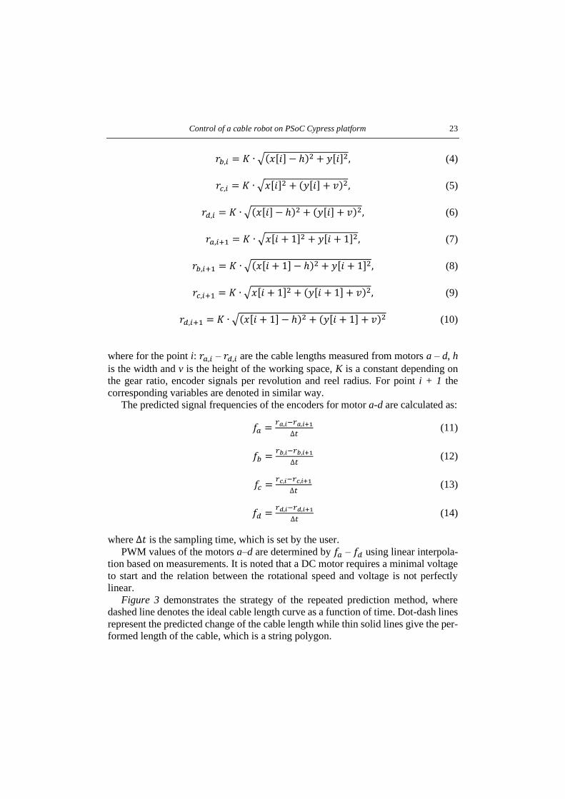
Figure 3 demonstrates the strategy of the repeated prediction method, where
dashed line denotes the ideal cable length curve as a function of time. Dot-dash lines
represent the predicted change of the cable length while thin solid lines give the per-
formed length of the cable, which is a string polygon.
24 Pálma Kapitány–József Lénárt
Figure 3. Strategy of the repeated prediction method
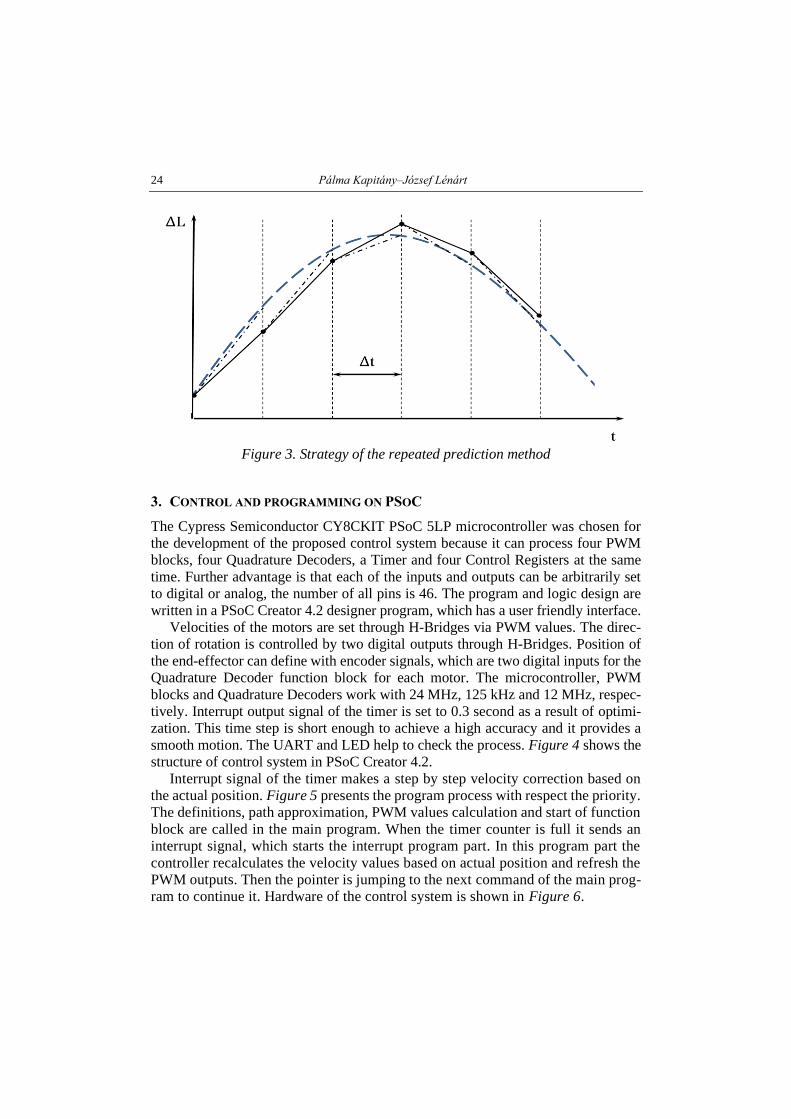
3. CONTROL AND PROGRAMMING ON PSOC
The Cypress Semiconductor CY8CKIT PSoC 5LP microcontroller was chosen for
the development of the proposed control system because it can process four PWM
blocks, four Quadrature Decoders, a Timer and four Control Registers at the same
time. Further advantage is that each of the inputs and outputs can be arbitrarily set
to digital or analog, the number of all pins is 46. The program and logic design are
written in a PSoC Creator 4.2 designer program, which has a user friendly interface.
Velocities of the motors are set through H-Bridges via PWM values. The direc-
tion of rotation is controlled by two digital outputs through H-Bridges. Position of
the end-effector can define with encoder signals, which are two digital inputs for the
Quadrature Decoder function block for each motor. The microcontroller, PWM
blocks and Quadrature Decoders work with 24 MHz, 125 kHz and 12 MHz, respec-
tively. Interrupt output signal of the timer is set to 0.3 second as a result of optimi-
zation. This time step is short enough to achieve a high accuracy and it provides a
smooth motion. The UART and LED help to check the process. Figure 4 shows the
structure of control system in PSoC Creator 4.2.
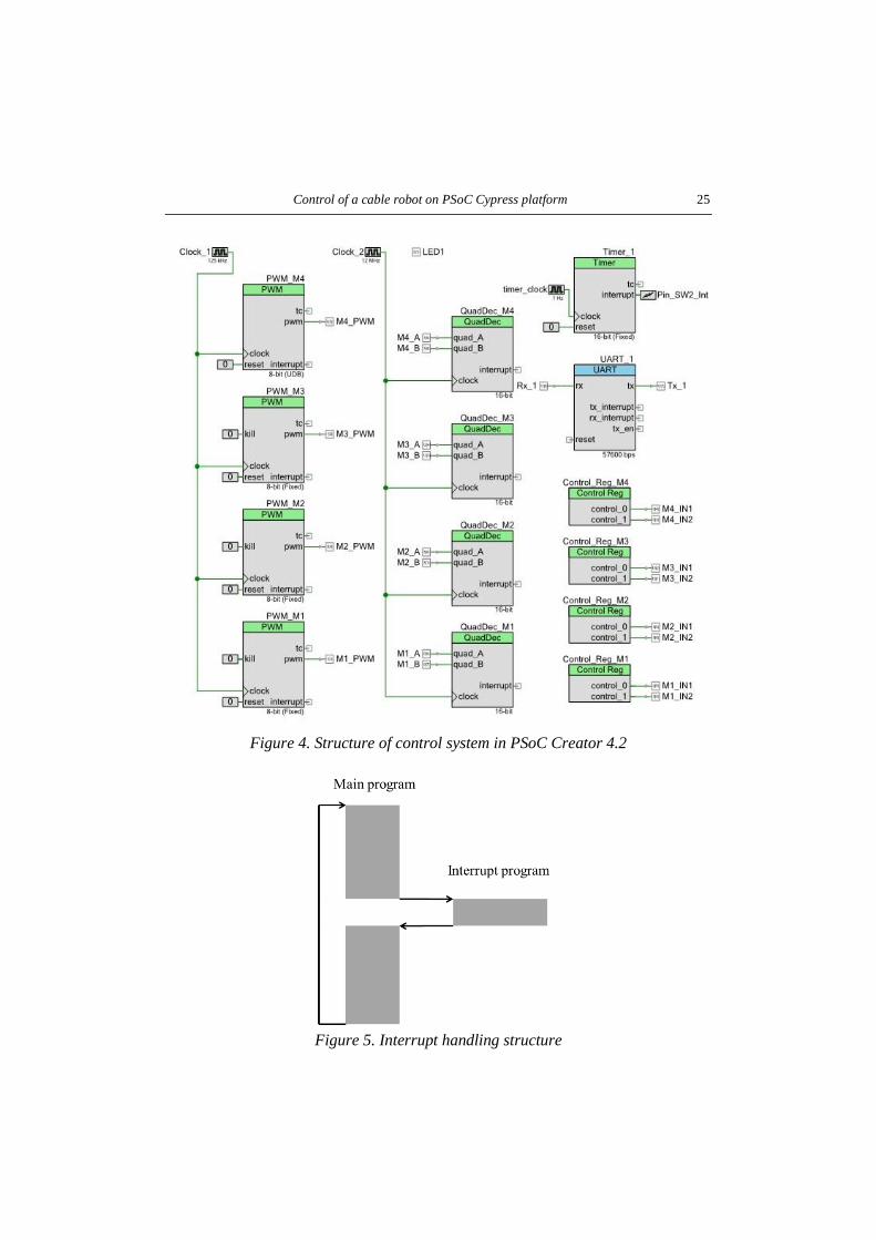
Interrupt signal of the timer makes a step by step velocity correction based on
the actual position. Figure 5 presents the program process with respect the priority.
The definitions, path approximation, PWM values calculation and start of function
block are called in the main program. When the timer counter is full it sends an
interrupt signal, which starts the interrupt program part. In this program part the
controller recalculates the velocity values based on actual position and refresh the
PWM outputs. Then the pointer is jumping to the next command of the main prog-
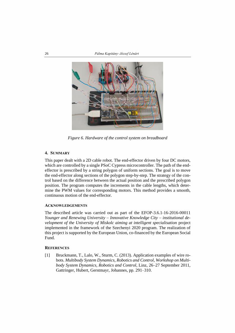
ram to continue it. Hardware of the control system is shown in Figure 6.
Control of a cable robot on PSoC Cypress platform 25
Figure 4. Structure of control system in PSoC Creator 4.2
Figure 5. Interrupt handling structure
26 Pálma Kapitány–József Lénárt
Figure 6. Hardware of the control system on breadboard
4. SUMMARY
This paper dealt with a 2D cable robot. The end-effector driven by four DC motors,
which are controlled by a single PSoC Cypress microcontroller. The path of the end-
effector is prescribed by a string polygon of uniform sections. The goal is to move
the end-effector along sections of the polygon step-by-step. The strategy of the con-
trol based on the difference between the actual position and the prescribed polygon
position. The program computes the increments in the cable lengths, which deter-
mine the PWM values for corresponding motors. This method provides a smooth,
continuous motion of the end-effector.
ACKNOWLEDGEMENTS
The described article was carried out as part of the EFOP-3.6.1-16-2016-00011
Younger and Renewing University – Innovative Knowledge City – institutional de-
velopment of the University of Miskolc aiming at intelligent specialisation project
implemented in the framework of the Szechenyi 2020 program. The realization of
this project is supported by the European Union, co-financed by the European Social
Fund.
REFERENCES
[1] Bruckmann, T., Lalo, W., Sturm, C. (2013). Application examples of wire ro-
bots. Multibody System Dynamics, Robotics and Control, Workshop on Multi-
body System Dynamics, Robotics and Control, Linz, 26–27 September 2011,
Gattringer, Hubert, Gerstmayr, Johannes, pp. 291–310.
Control of a cable robot on PSoC Cypress platform 27
[2] Kapitány, P., Lénárt, J. (2019). Kinematics and control of a planar cable robot.
International Journal of Engineering and Management Sciences (IJEMS),
Vol. 4, No. 1, pp. 88–95.
[3] Bruckmann, T., Pott, A., Franitza, D., Hiller, M. (2006). A Modular Controller
for Redundantly Actuated Tendon-Based Stewart Platforms. The first Euro-
pean Conference on Mechanism Science, Obergurgl, Austria, 21–26 February
2006.
[4] Jadhao, K. S., Lambert, P., Bruckmann, T., Herder, J. L. (2018). Design and
Analysis of a Novel Cable-Driven Haptic Master Device for Planar Grasping.
In: Gosselin, C., Cardou, P., Bruckmann, T., Pott, A. Cable-Driven Parallel
Robots. Mechanisms and Machine Science. Vol. 5, Cham, Switzerland.
[5] Xue Jun Jin, Dae Ik Jun, Pott, A., Sukho Park, Jong-Oh Park, Seong Young
Ko (2013). Four-cable-driven parallel robot. 13th International Conference on
Control, Automation and Systems, Kimdaejung Convention Center, Gwangju,
Korea.
[6] Gosselin, C., Ren, P.,Foucault, Simon (2012). Dynamic Trajectory Planning
of a Two-DOF Cable-Suspended Parallel Robot. Proceedings – IEEE Inter-
national Conference on Robotics and Automation, pp. 1476–1481, 10.1109/
ICRA.2012.6224683.
[7] Gosselin, C., Foucault, S. (2015). Experimental Determination of the Accu-
racy of a Three-Dof Cable-Suspended Parallel Robot Performing Dynamic
Trajectories. Mechanisms and Machine Science, 32, pp. 101–112, 10.1007/
978-3-319-09489-2_8.
[8] Lau, D., Hawke, T., Kempton, L., Oetomo, D., Halgamuge, S. (2010). Design
and Analysis of 4-DOF Cable-Driven Parallel Mechanism. Proceedings of the
2010 Australasian Conference on Robotics and Automation.
Design of Machines and Structures, Vol. 10, No. 1 (2020), pp. 28–38.
Doi: 10.32972/dms.2020.004
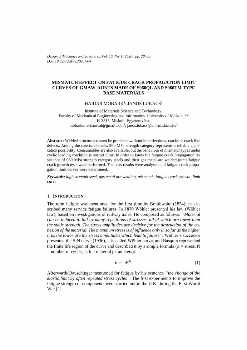
MISMATCH EFFECT ON FATIGUE CRACK PROPAGATION LIMIT
CURVES OF GMAW JOINTS MADE OF S960QL AND S960TM TYPE
BASE MATERIALS
HAIDAR MOBARK1–JÁNOS LUKÁCS2
Institute of Materials Science and Technology,
Faculty of Mechanical Engineering and Informatics, University of Miskolc 1, 2
H-3515, Miskolc-Egyetemváros
[email protected], [email protected]
Abstract: Welded structures cannot be produced without imperfections, cracks or crack like
defects. Among the structural steels, 960 MPa strength category represents a reliable appli-
cation possibility. Consumables are also available, but the behaviour of mismatch types under
cyclic loading condition is not yet clear. In order to know the fatigue crack propagation re-
sistance of 960 MPa strength category steels and their gas metal arc welded joints fatigue
crack growth tests were performed. The tests results were analysed and fatigue crack propa-
gation limit curves were determined.
Keywords: high strength steel, gas metal arc welding, mismatch, fatigue crack growth, limit
curve
1. INTRODUCTION
The term fatigue was mentioned for the first time by Braithwaite (1854); he de-
scribed many service fatigue failures. In 1870 Wӧhler presented his law (Wӧhler
law), based on investigations of railway axles. He composed as follows: “Material
can be induced to fail by many repetitions of stresses, all of which are lower than
the static strength. The stress amplitudes are decisive for the destruction of the co-
hesion of the material. The maximum stress is of influence only in so far as the higher
it is, the lower are the stress amplitudes which lead to failure”. Wӧhler’s successor
presented the S-N curve (1936), it is called Wӧhler curve, and Basquin represented
the finite life region of the curve and described it by a simple formula ( = stress, N
= number of cycles, a, b = material parameters):
σ = aNb. (1)
Afterwards Bauschinger mentioned for fatigue by his sentence “the change of the
elastic limit by often repeated stress cycles”. The first experiments to improve the
fatigue strength of components were carried out in the U.K. during the First World
War [1].
Mismatch effect on fatigue crack propagation limit curves of GMAW joints made of S960QL and…29
From 1960 onwards the number of fatigue experts increased still further. This
must also be attributed to the rapid development of fracture mechanics, i.e. of fa-
tigue-crack propagation. Paris established that fatigue crack propagation could be
described by the following equation (da/dN = fatigue crack growth, K = stress in-
tensity factor range, C, n = material constants) [2, 3]:
da
dN= C∆Kn, (2)
which equation soon set out on a veritable triumphant advance around the world [1].
The complex process of crack propagation is undoubtedly described much too
simply by this equation; this fact however did not prevent its – either undiscriminat-
ing or adding further characteristics – use all over the world to this very day.
The most commonly used structural material for the construction of engineering
structures is steel, and the most widely used joining technology is welding. Nowa-
days, steel providers create a modern version of a high-strength base materials and
filler metals with yield strength start from 690 MPa and up. However, high strength
lightweight structures with low cost of steel weldments lead to apply in many man-
ufacturing aspects (e.g. mobile cranes, hydropower plants, offshores, trucks, earth-
moving machines, and drums), because of an extensive reduction in weight [4].
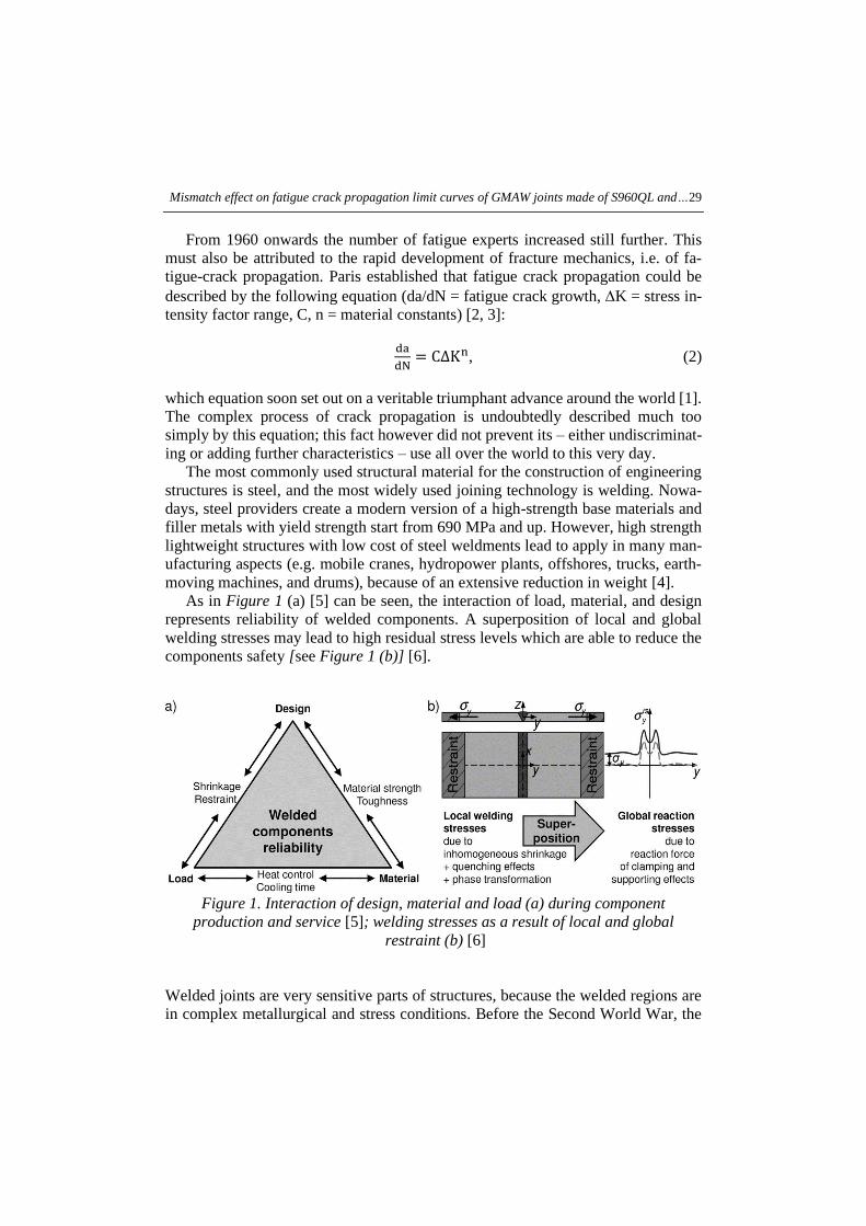
As in Figure 1 (a) [5] can be seen, the interaction of load, material, and design
represents reliability of welded components. A superposition of local and global
welding stresses may lead to high residual stress levels which are able to reduce the
components safety [see Figure 1 (b)] [6].
Figure 1. Interaction of design, material and load (a) during component
production and service [5]; welding stresses as a result of local and global
restraint (b) [6]
Welded joints are very sensitive parts of structures, because the welded regions are
in complex metallurgical and stress conditions. Before the Second World War, the
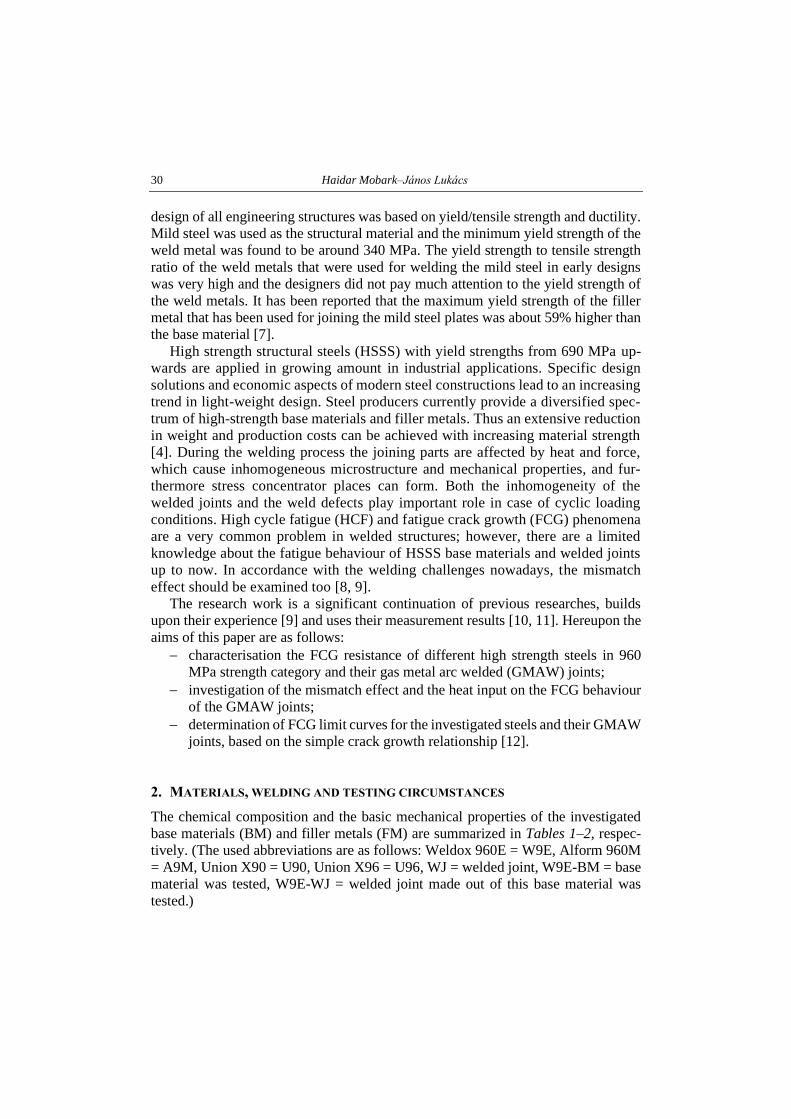
30 Haidar Mobark–János Lukács
design of all engineering structures was based on yield/tensile strength and ductility.
Mild steel was used as the structural material and the minimum yield strength of the
weld metal was found to be around 340 MPa. The yield strength to tensile strength
ratio of the weld metals that were used for welding the mild steel in early designs
was very high and the designers did not pay much attention to the yield strength of
the weld metals. It has been reported that the maximum yield strength of the filler
metal that has been used for joining the mild steel plates was about 59% higher than
the base material [7].
High strength structural steels (HSSS) with yield strengths from 690 MPa up-
wards are applied in growing amount in industrial applications. Specific design
solutions and economic aspects of modern steel constructions lead to an increasing
trend in light-weight design. Steel producers currently provide a diversified spec-
trum of high-strength base materials and filler metals. Thus an extensive reduction
in weight and production costs can be achieved with increasing material strength
[4]. During the welding process the joining parts are affected by heat and force,
which cause inhomogeneous microstructure and mechanical properties, and fur-
thermore stress concentrator places can form. Both the inhomogeneity of the
welded joints and the weld defects play important role in case of cyclic loading
conditions. High cycle fatigue (HCF) and fatigue crack growth (FCG) phenomena
are a very common problem in welded structures; however, there are a limited
knowledge about the fatigue behaviour of HSSS base materials and welded joints
up to now. In accordance with the welding challenges nowadays, the mismatch
effect should be examined too [8, 9].
The research work is a significant continuation of previous researches, builds
upon their experience [9] and uses their measurement results [10, 11]. Hereupon the
aims of this paper are as follows:
− characterisation the FCG resistance of different high strength steels in 960
MPa strength category and their gas metal arc welded (GMAW) joints;
− investigation of the mismatch effect and the heat input on the FCG behaviour
of the GMAW joints;
− determination of FCG limit curves for the investigated steels and their GMAW
joints, based on the simple crack growth relationship [12].
2. MATERIALS, WELDING AND TESTING CIRCUMSTANCES
The chemical composition and the basic mechanical properties of the investigated
base materials (BM) and filler metals (FM) are summarized in Tables 1–2, respec-
tively. (The used abbreviations are as follows: Weldox 960E = W9E, Alform 960M
= A9M, Union X90 = U90, Union X96 = U96, WJ = welded joint, W9E-BM = base
material was tested, W9E-WJ = welded joint made out of this base material was
tested.)
Mismatch effect on fatigue crack propagation limit curves of GMAW joints made of S960QL and…31
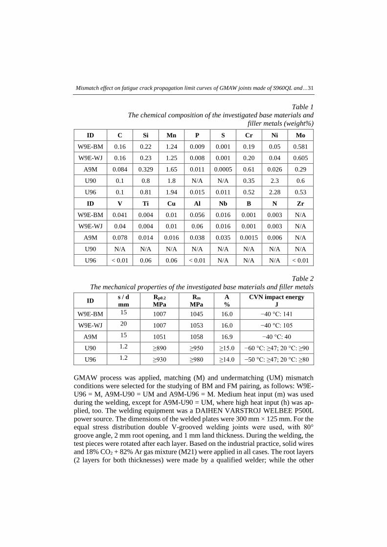
Table 1
The chemical composition of the investigated base materials and
filler metals (weight%)
ID C Si Mn P S Cr Ni Mo
W9E-BM 0.16 0.22 1.24 0.009 0.001 0.19 0.05 0.581
W9E-WJ 0.16 0.23 1.25 0.008 0.001 0.20 0.04 0.605
A9M 0.084 0.329 1.65 0.011 0.0005 0.61 0.026 0.29
U90 0.1 0.8 1.8 N/A N/A 0.35 2.3 0.6
U96 0.1 0.81 1.94 0.015 0.011 0.52 2.28 0.53
ID V Ti Cu Al Nb B N Zr
W9E-BM 0.041 0.004 0.01 0.056 0.016 0.001 0.003 N/A
W9E-WJ 0.04 0.004 0.01 0.06 0.016 0.001 0.003 N/A
A9M 0.078 0.014 0.016 0.038 0.035 0.0015 0.006 N/A
U90 N/A N/A N/A N/A N/A N/A N/A N/A
U96 < 0.01 0.06 0.06 < 0.01 N/A N/A N/A < 0.01
Table 2
The mechanical properties of the investigated base materials and filler metals
ID s / d
mm
Rp0.2
MPa
Rm
MPa
A
%
CVN impact energy
J
W9E-BM 15 1007 1045 16.0 −40 °C: 141
W9E-WJ 20 1007 1053 16.0 −40 °C: 105
A9M 15 1051 1058 16.9 −40 °C: 40
U90 1.2 ≥890 ≥950 ≥15.0 −60 °C: ≥47; 20 °C: ≥90
U96 1.2 ≥930 ≥980 ≥14.0 −50 °C: ≥47; 20 °C: ≥80
GMAW process was applied, matching (M) and undermatching (UM) mismatch
conditions were selected for the studying of BM and FM pairing, as follows: W9E-
U96 = M, A9M-U90 = UM and A9M-U96 = M. Medium heat input (m) was used
during the welding, except for A9M-U90 = UM, where high heat input (h) was ap-
plied, too. The welding equipment was a DAIHEN VARSTROJ WELBEE P500L
power source. The dimensions of the welded plates were 300 mm × 125 mm. For the
equal stress distribution double V-grooved welding joints were used, with 80°
groove angle, 2 mm root opening, and 1 mm land thickness. During the welding, the
test pieces were rotated after each layer. Based on the industrial practice, solid wires
and 18% CO2 + 82% Ar gas mixture (M21) were applied in all cases. The root layers
(2 layers for both thicknesses) were made by a qualified welder; while the other
32 Haidar Mobark–János Lukács
layers (6 layers for 15 mm and 10 layers for 20 mm thicknesses) were made by au-
tomated welding car. The welding parameters (preheating and interpass temperatures
(Tpre and Tip), current (I), voltage (U), welding speed (vw), linear energy Ev), cooling
time (t8.5/5)) were selected based on both theoretical considerations and real industrial
applications, and were summarized in Table 3. (The used abbreviations are as fol-
lows: root = r, filler = f).
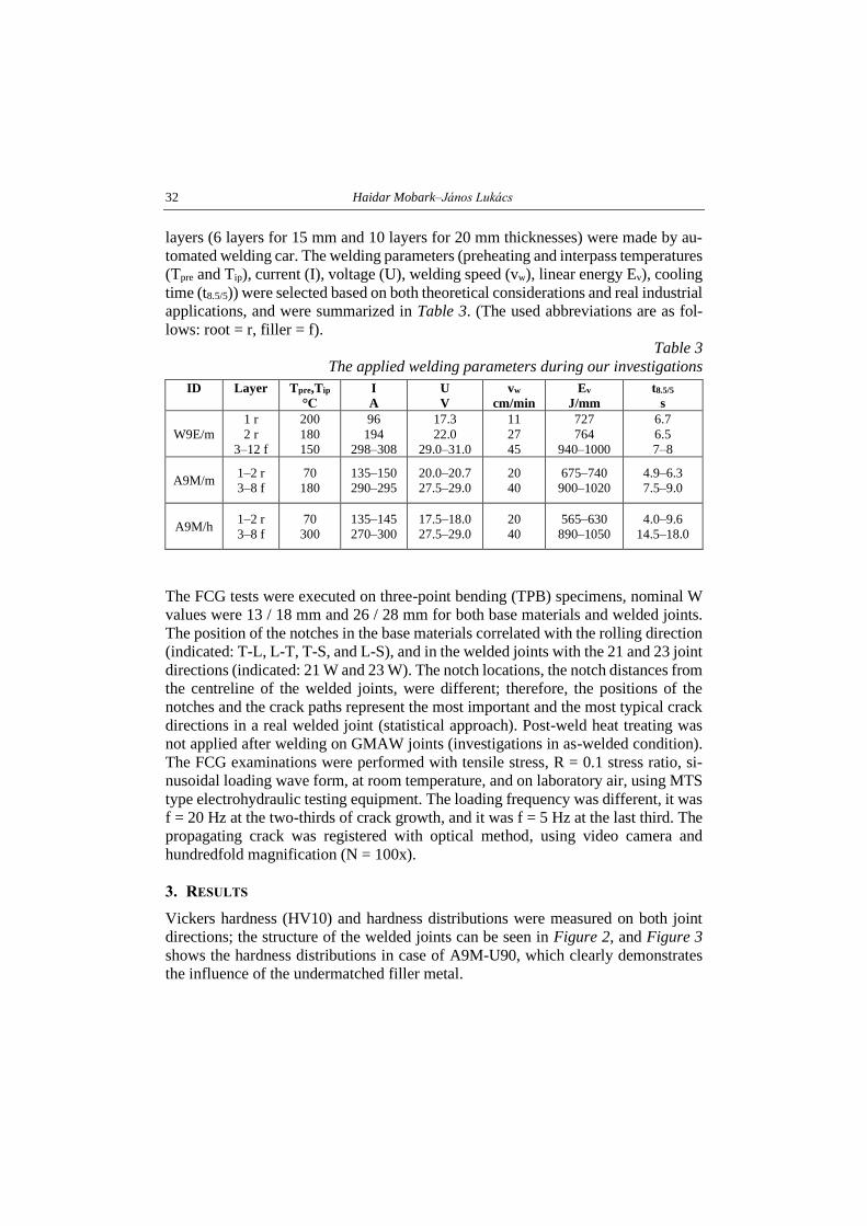
Table 3
The applied welding parameters during our investigations
ID Layer Tpre,Tip
°C
I
A
U
V
vw
cm/min
Ev
J/mm
t8.5/5
s
W9E/m
1 r
2 r
3–12 f
200
180
150
96
194
298–308
17.3
22.0
29.0–31.0
11
27
45
727
764
940–1000
6.7
6.5
7–8
A9M/m 1–2 r
3–8 f
70
180
135–150
290–295
20.0–20.7
27.5–29.0
20
40
675–740
900–1020
4.9–6.3
7.5–9.0
A9M/h 1–2 r
3–8 f
70
300
135–145
270–300
17.5–18.0
27.5–29.0
20
40
565–630
890–1050
4.0–9.6
14.5–18.0
The FCG tests were executed on three-point bending (TPB) specimens, nominal W
values were 13 / 18 mm and 26 / 28 mm for both base materials and welded joints.
The position of the notches in the base materials correlated with the rolling direction
(indicated: T-L, L-T, T-S, and L-S), and in the welded joints with the 21 and 23 joint
directions (indicated: 21 W and 23 W). The notch locations, the notch distances from
the centreline of the welded joints, were different; therefore, the positions of the
notches and the crack paths represent the most important and the most typical crack
directions in a real welded joint (statistical approach). Post-weld heat treating was
not applied after welding on GMAW joints (investigations in as-welded condition).
The FCG examinations were performed with tensile stress, R = 0.1 stress ratio, si-
nusoidal loading wave form, at room temperature, and on laboratory air, using MTS
type electrohydraulic testing equipment. The loading frequency was different, it was
f = 20 Hz at the two-thirds of crack growth, and it was f = 5 Hz at the last third. The
propagating crack was registered with optical method, using video camera and
hundredfold magnification (N = 100x).
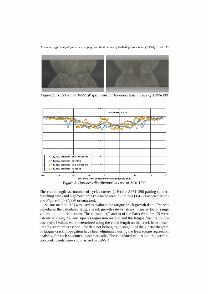
3. RESULTS
Vickers hardness (HV10) and hardness distributions were measured on both joint
directions; the structure of the welded joints can be seen in Figure 2, and Figure 3
shows the hardness distributions in case of A9M-U90, which clearly demonstrates
the influence of the undermatched filler metal.
Mismatch effect on fatigue crack propagation limit curves of GMAW joints made of S960QL and…33
Figure 2. T-L/21W and T-S/23W specimens for hardness tests in case of A9M-U90
Figure 3. Hardness distributions in case of A9M-U90
The crack length vs. number of cycles curves (a-N) for A9M-U90 pairing (under-
matching case) and high heat input (h) can be seen in Figure 4 (T-L/21W orientation)
and Figure 5 (T-S/23W orientation).
Secant method [13] was used to evaluate the fatigue crack growth data. Figure 6
introduces the calculated fatigue crack growth rate vs. stress intensity factor range
values, in both orientations. The constants (C and n) of the Paris equation (2) were
calculated using the least squares regression method and the fatigue fracture tough-
ness (ΔKfc) values were determined using the crack length on the crack front meas-
ured by stereo microscope. The data not belonging to stage II of the kinetic diagram
of fatigue crack propagation have been eliminated during the least square regression
analysis, for each specimen, systematically. The calculated values and the correla-
tion coefficients were summarized in Table 4.
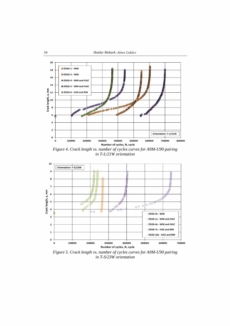
34 Haidar Mobark–János Lukács
Figure 4. Crack length vs. number of cycles curves for A9M-U90 pairing
in T-L/21W orientation
Figure 5. Crack length vs. number of cycles curves for A9M-U90 pairing
in T-S/23W orientation
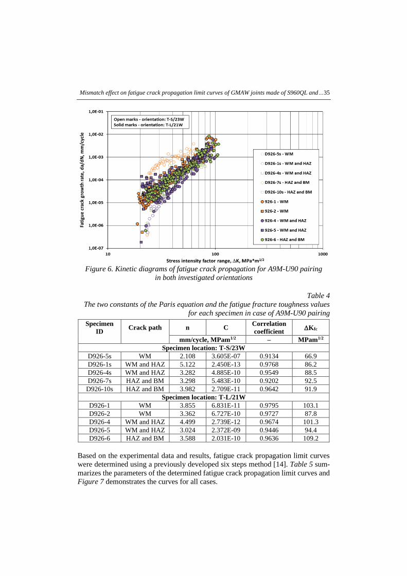
Mismatch effect on fatigue crack propagation limit curves of GMAW joints made of S960QL and…35
Figure 6. Kinetic diagrams of fatigue crack propagation for A9M-U90 pairing
in both investigated orientations
Table 4
The two constants of the Paris equation and the fatigue fracture toughness values
for each specimen in case of A9M-U90 pairing
Specimen
ID Crack path n C
Correlation
coefficient Kfc
mm/cycle, MPam1/2 – MPam1/2
Specimen location: T-S/23W
D926-5s WM 2.108 3.605E-07 0.9134 66.9
D926-1s WM and HAZ 5.122 2.450E-13 0.9768 86.2
D926-4s WM and HAZ 3.282 4.885E-10 0.9549 88.5
D926-7s HAZ and BM 3.298 5.483E-10 0.9202 92.5
D926-10s HAZ and BM 3.982 2.709E-11 0.9642 91.9
Specimen location: T-L/21W
D926-1 WM 3.855 6.831E-11 0.9795 103.1
D926-2 WM 3.362 6.727E-10 0.9727 87.8
D926-4 WM and HAZ 4.499 2.739E-12 0.9674 101.3
D926-5 WM and HAZ 3.024 2.372E-09 0.9446 94.4
D926-6 HAZ and BM 3.588 2.031E-10 0.9636 109.2
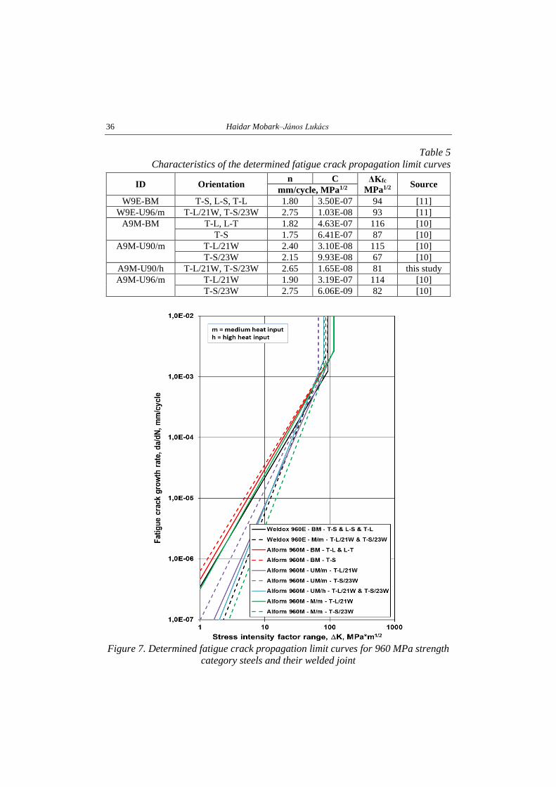
Based on the experimental data and results, fatigue crack propagation limit curves
were determined using a previously developed six steps method [14]. Table 5 sum-
marizes the parameters of the determined fatigue crack propagation limit curves and
Figure 7 demonstrates the curves for all cases.
36 Haidar Mobark–János Lukács
Table 5
Characteristics of the determined fatigue crack propagation limit curves
ID Orientation n C ΔKfc
MPa1/2 Source
mm/cycle, MPa1/2
W9E-BM T-S, L-S, T-L 1.80 3.50E-07 94 [11]
W9E-U96/m T-L/21W, T-S/23W 2.75 1.03E-08 93 [11]
A9M-BM T-L, L-T 1.82 4.63E-07 116 [10]
T-S 1.75 6.41E-07 87 [10]
A9M-U90/m T-L/21W 2.40 3.10E-08 115 [10]
T-S/23W 2.15 9.93E-08 67 [10]
A9M-U90/h T-L/21W, T-S/23W 2.65 1.65E-08 81 this study
A9M-U96/m T-L/21W 1.90 3.19E-07 114 [10]
T-S/23W 2.75 6.06E-09 82 [10]
Figure 7. Determined fatigue crack propagation limit curves for 960 MPa strength
category steels and their welded joint
Mismatch effect on fatigue crack propagation limit curves of GMAW joints made of S960QL and…37
4. Summary and conclusions
Based on our investigations, the calculated and analysed testing results, and the ac-
complished comparisons, the following conclusions can be drawn.
The results of the achieved fatigue crack growth investigations justified the ne-
cessity of statistical approaches, especially referring to the directions of the base
materials and the welded joints, and the determination of the number of the tested
specimens.
The applied gas metal arc welding process and the used technological parameters
are suitable for production welded joints with appropriate quality, where the appro-
priate quality contains the eligible resistance to fatigue crack propagation too.
The fatigue crack growth resistance of the investigated base materials is different
in different crack path directions, which depends on the material grade too.
The welding causes unfavourable effects both on the mechanical properties and
the fatigue crack growth resistance of the high strength steels.
Based on these results and the used methods, fatigue crack propagation limit
curves can be determined for the investigated high strength steel base materials and
their gas metal arc welded joints.
The selected values of the Paris exponents (n) for the fatigue crack propagation
limit curves of the investigated welded joints were higher than the exponents of the
concerning base materials, in both mismatch conditions.
Both the mismatch condition and the heat input have significant effects on the fa-
tigue crack growth characteristics on the investigated high strength steel welded joints.
The limit curves on the one hand correctly reflect the fatigue crack growth char-
acteristics of both the base materials and the welded joints, on the other hand are
usable for structural integrity and/or reliability assessment calculations.
The research work should be continued. Further examinations and analyses re-
quired in order to draw statistically better established conclusions, to measure thresh-
old stress intensity factor range (ΔKth) values for base materials and welded joints,
to reveal the influence of the welding technological parameters and finally, to study
the effects of the welding residual stress fields.
REFERENCES
[1] Schütz, W. (1996). A history of fatigue. Engineering Fracture Mechanics,
Vol. 54, No. 2, pp. 263–300, ISSN 0013-7944.
[2] Paris, P. C., Gomez, M. P., Anderson, W. E. (1961). A rational analytic theory
of fatigue. The Trend in Engineering, Vol. 13, pp. 9–14.
[3] Paris, P., Erdogan, F. (1963). A critical analysis of crack propagation laws.
Journal of Basic Engineering, Vol. 85, pp. 528–533.
[4] Schroepfer, D., Kannengiesser, T. (2016). Stress build-up in HSLA steel
welds due to material behavior. Journal of Materials Processing Technology,
Vol. 227, pp. 49–58, ISSN 0924-0136.
38 Haidar Mobark–János Lukács
[5] Lausch, T., Kannengiesser, T., Schmitz-Niederau, M. (2013). Multi-axial load
analysis of thick-walled component welds made of 13CrMoV9-10. Journal of
Materials Processing Technology, Vol. 213, pp. 1234–1240, ISSN 0924-
0136.
[6] Schroepfer, D., Kromm, A., Kannengiesser, T. (2015). Improving welding
stresses by filler metal and heat control selection in component-related butt
joints of high-strength steel. Welding in the World, Vol. 59, No. 3, pp. 455–
464, ISSN 0043-2288.
[7] Ravi, S., Balasubramanian, V., Nemat Nasser, S. (2004). Effect of mis-match
ratio (MMR) on fatigue crack growth behaviour of HSLA steel welds. Engi-
neering Failure Analysis, Vol. 11, No. 3, pp. 413–428, June 2004, ISSN 1350-
6307.
[8] Mobark, H. F. M., Lukács, J. (2018). Mismatch effect influence on the high
cycle fatigue resistance of S690QL type high strength steels. 2nd International
Conference on Structural Integrity and Durability, Dubrovnik, Croatia, Octo-
ber 2–5.
[9] Balogh, A., Lukács, J., Török, I. (eds.) (2015). Weldability and the Properties
of the Welded Joints. University of Miskolc, Miskolc, p. 324 (In Hungarian),
ISBN 9789633580813.
[10] Dobosy, Á. (2017). Design limit curves for cyclic loaded structural elements
made of high strength steels. PhD Thesis, István Sályi Doctoral School of
Mechanical Engineering Sciences, University of Miskolc, Miskolc (In Hun-
garian).
[11] Gáspár, M. (2016). Welding technology development of Q+T high strength
steels based on physical simulation. PhD Thesis, István Sályi Doctoral School
of Mechanical Engineering Sciences, University of Miskolc, Miskolc, (In
Hungarian).
[12] BS 7910:2013+A1:2015: Guide to methods for assessing the acceptability of
flaws in metallic structures. BSI Standards Limited, 2015.
[13] ASTM E647-15e1: Standard Test Method for Measurement of Fatigue Crack
Growth Rate. ASTM International, 2015.
[14] Lukács, J. (2003). Fatigue crack propagation limit curves for different metallic
and non-metallic materials. Materials Science Forum, Vol. 414–415, pp. 31–
36, ISSN 1662-9752.
Design of Machines and Structures, Vol. 10, No. 1 (2020), pp. 39–48.
Doi: 10.32972/dms.2020.005
DEVELOPMENT OF AN ELECTRIC MEASUREMENT SYSTEM
FOR RAPID DETERMINATION OF THE FRICTION COEFFICIENT
LÁSZLÓ RÓNAI
University of Miskolc, Robert Bosch Department of Mechatronics
3515, Miskolc-Egyetemváros
Abstract: Development of an electric measurement system for rapid determination of the
friction coefficient is discussed in this paper. The electric system is capable to use with a ball
cage guide bush unit. Two beam load cells are included into the system and the measured
values of the forces are processed by microcontrollers. In the course of measurements, nor-
mal- and tangential forces of inner or outer surfaces of different enamelled specimens could
be determined. A data acquisition program is developed to record the force values to a per-
sonal computer. Linear interpolation method is required to synchronize the values of the load
cells, which is necessary to calculate the coefficient of friction.
Keywords: friction coefficient, microcontroller, Arduino
1. INTRODUCTION
The friction as phenomenon can be experienced in everyday life. The behaviour of
mechanical systems, which contain moving parts, strongly influenced by the friction
[1]. There are several friction models, e.g. Dahl, viscous, Stribeck model, etc., which
can be used for different aspects [1], [2]. The most common model is the Coulomb
model of friction, which deals with the dry friction. In many problems, this model is
adequate to use.
The so-called friction coefficient can be measured experimentally with different
methods. The static and kinetic friction coefficients can be calculated with use of an
inclined plane [3], [4]. These experimental setups consist a slope and its angle can
be varied. Due to the change of the angle, the specimen may begin to tilt on the plane.
When the specimen starts to move, the current angle of the inclined plane provides
the static friction coefficient. In [5] an experimental setup contains a S-shaped load
cell, which used to measure the tensile force of the friction.
The main purpose of the paper is to develop an electrical device for the measure-
ment system, which is capable to use for rapid and approximate determination of the
friction coefficient. Mechanical design of the construction is detailed and summa-
rized in [6]. Internal and external surfaces of the measured specimens, e.g., enam-
elled aerosol cans, have different friction coefficients. The measurement system con-
tains two load cells, three Arduino Nano prototype board with AVR type AT-
mega328 microcontrollers [7], two A/D converters, and two transmission sensors.
40 László Rónai
This paper is organized as follows: Section 2 contains the designing aspects of
the electrical system and describes the whole device. Section 3 deals with the pro-
grams developed for the microcontrollers and for a laptop. Section 4 details the de-
termination of the friction coefficient. A special purpose program is developed to
use the linear interpolation method to synchronize the values of the load cells for the
same timestamp. A test measurement is also demonstrated. The Section 5 has con-
cluding remarks.
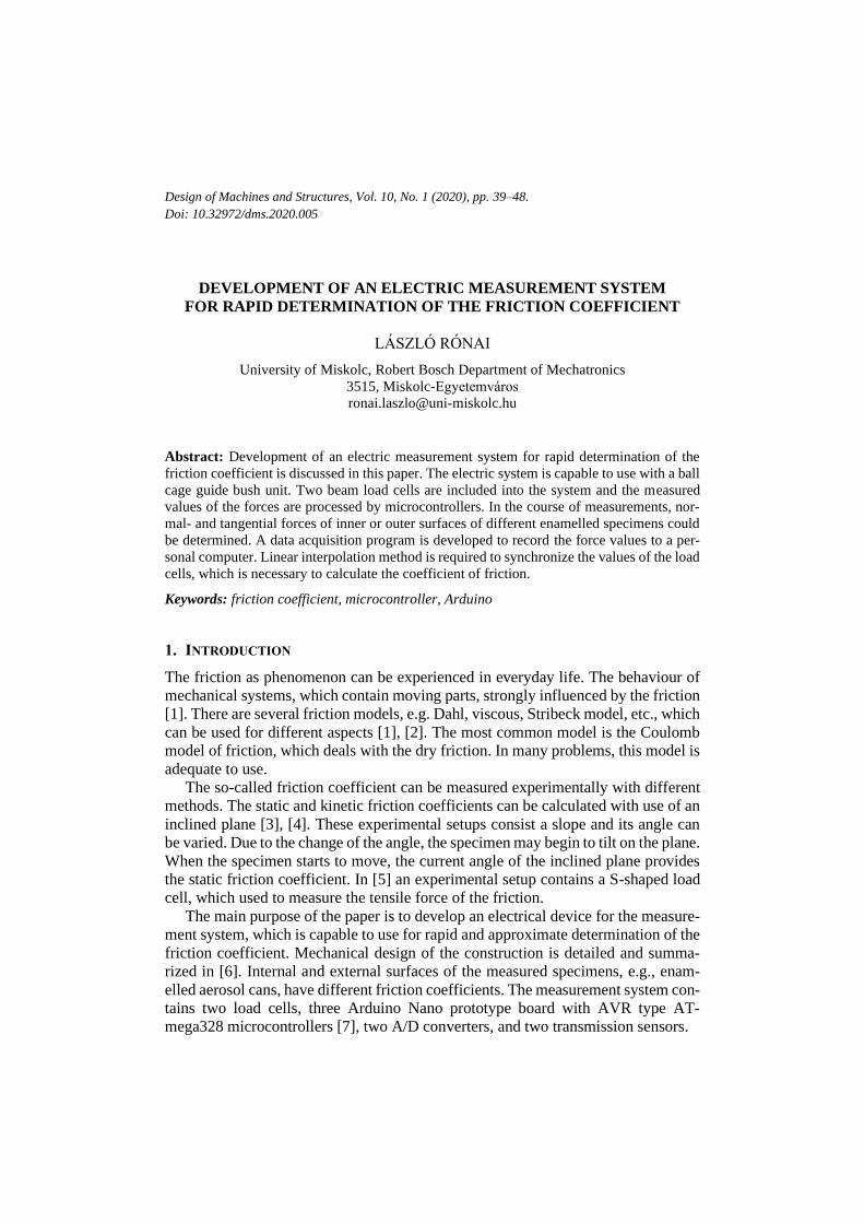
2. DESIGNING OF THE MEASUREMENT SYSTEM
The main function of the machine is to determine rapidly the friction coefficient. The
model of the unit is shown in Figure 1. A specimen of an aerosol can, which may
have different diameters can be fixed to a ball cage guide bush with a hold-down
element. The radial surface of a holder is manufactured to a revolver one. Therefore,
specimens can be inserted onto the holder with different diameters. Due to revolver
shaped holder the friction coefficients of the inner and outer surfaces of the cans can
be also measured. A steel tool, which is placed onto the specimen, is kept in a per-
manent position by a sheet metal in the course of the measurement.
The guide bush is moved with a handle manually. Since the measurement of both
normal- and tangential forces are required at the same time to determine the friction
coefficient, the system contains two beam shaped load cells. The tangential force is
measured by a load cell LC_t and the normal force is determined by another load
cell LC_n (see Figure 1). A predefined load in normal direction can be adjusted with
a winding knob. A ball bearing is in the bottom of LC_n to roll when the guide bush
is moved. The capacities of the above-mentioned load cells are different. The maxi-
mum allowable forces of LC_t and LC_n are 50 N and 200 N, respectively. The posi-
tive velocity of the guide bush is denoted by v+. A spring is added to the threaded shaft
to provide a relatively constant normal force during the measurement.
v+
LC_t
LC_n
tool
handle ball cage guide
bush unit
winding knob
hold-down element of the specimen
ball bearing
revolver type holder
sheet
metal
specimen
threaded shaft
Figure 1. Model of the measurement system
Development of an electric measurement system for rapid determination of the friction coefficient 41
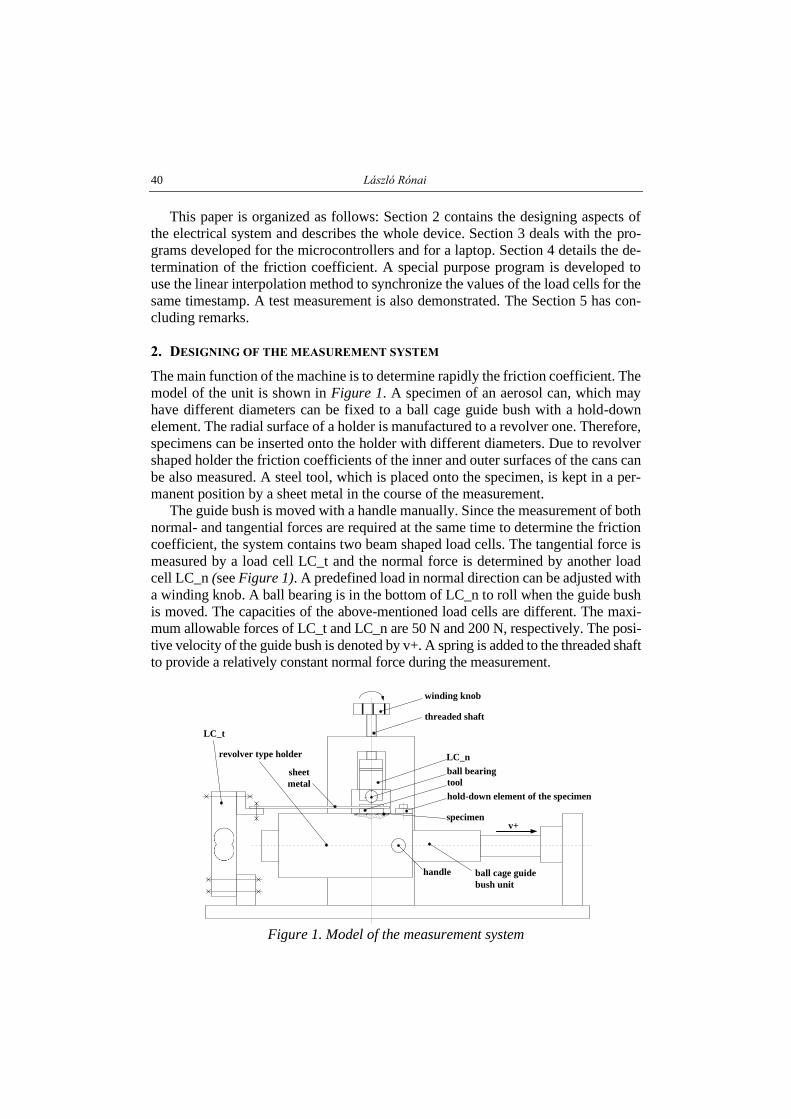
The block scheme of the electrical system is shown in Figure 2. A beam load cell
contains four strain gauges, which are wired to each other in a Wheatstone bridge
configuration. Due to bridge configuration the change of resistance is transformed
to change in the bridge voltage. The voltage can be measured by a HX711 type 24-
bit sigma-delta A/D converter [8] with 80 Hz sampling rate. The data are sent via
serial communication protocol to the microcontrollers MC 1 and MC 2. The forces
are determined by a self-devised program. Scaling of incoming data is performed by
the program. These values are transmitted to a laptop with UART communication
protocol.
Two transmissive sensors are used to calculate the average velocity of the guide
bush. These optical sensors have a phototransistor and an infrared emitter in a face-
to-face configuration. The elapsed time between the base and end position is meas-
ured by a microcontroller MC 3, which provide an average velocity in aware of the
distance:
�̅� =∆𝑥
∆𝑡=
79 𝑚𝑚
∆𝑡. (1)
Figure 2. Block scheme of the electric system
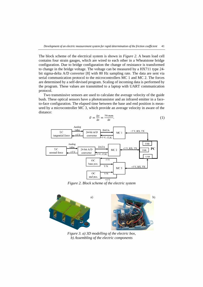
Figure 3. a) 3D modelling of the electric box,
b) Assembling of the electric components
42 László Rónai
The electric system and its box are designed in Autodesk Inventor software. The box
and its cap are manufactured by 3D printing technique using polylactic acid (PLA)
filament. Layers are 0.1 mm with rectilinear filling method prescribing 10% infill
parameter. The 3D model of the electric box is shown in Figure 3a and the manu-
factured one is given in Figure 3b. Three state LEDs with limiting resistors are also
built in the box.
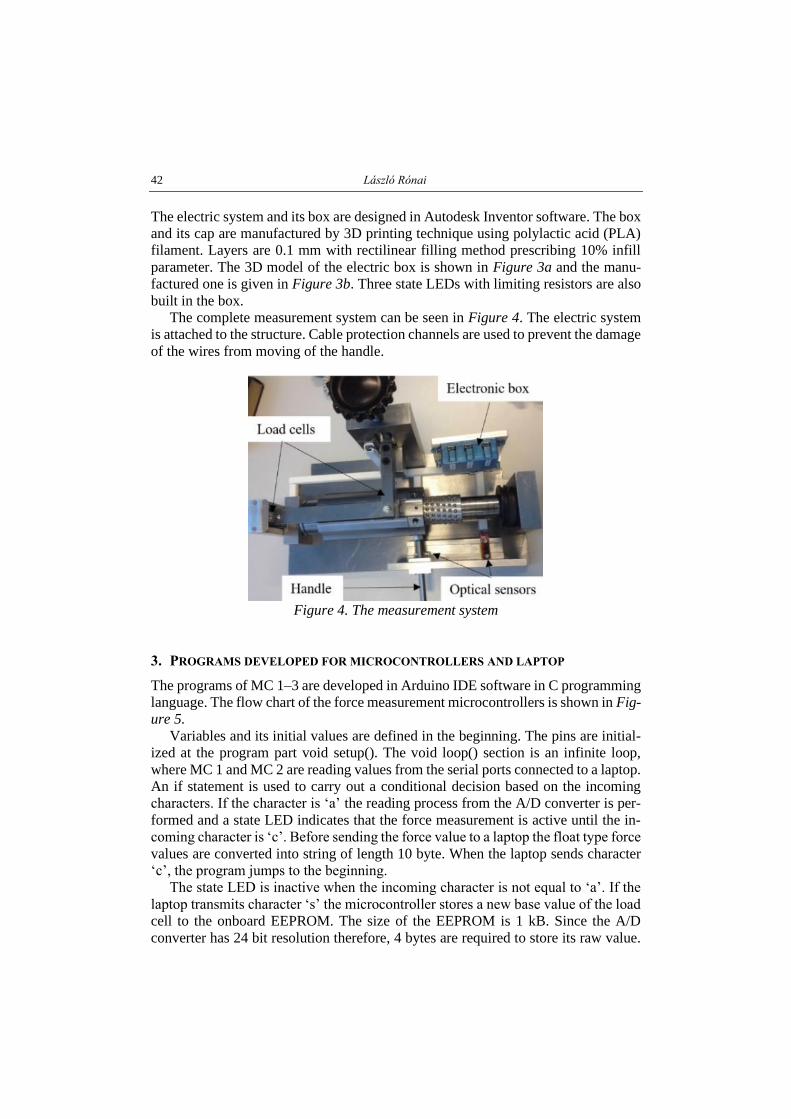
The complete measurement system can be seen in Figure 4. The electric system
is attached to the structure. Cable protection channels are used to prevent the damage
of the wires from moving of the handle.
Figure 4. The measurement system
3. PROGRAMS DEVELOPED FOR MICROCONTROLLERS AND LAPTOP
The programs of MC 1–3 are developed in Arduino IDE software in C programming
language. The flow chart of the force measurement microcontrollers is shown in Fig-
ure 5.
Variables and its initial values are defined in the beginning. The pins are initial-
ized at the program part void setup(). The void loop() section is an infinite loop,
where MC 1 and MC 2 are reading values from the serial ports connected to a laptop.
An if statement is used to carry out a conditional decision based on the incoming
characters. If the character is ‘a’ the reading process from the A/D converter is per-
formed and a state LED indicates that the force measurement is active until the in-
coming character is ‘c’. Before sending the force value to a laptop the float type force
values are converted into string of length 10 byte. When the laptop sends character
‘c’, the program jumps to the beginning.
The state LED is inactive when the incoming character is not equal to ‘a’. If the
laptop transmits character ‘s’ the microcontroller stores a new base value of the load
cell to the onboard EEPROM. The size of the EEPROM is 1 kB. Since the A/D
converter has 24 bit resolution therefore, 4 bytes are required to store its raw value.
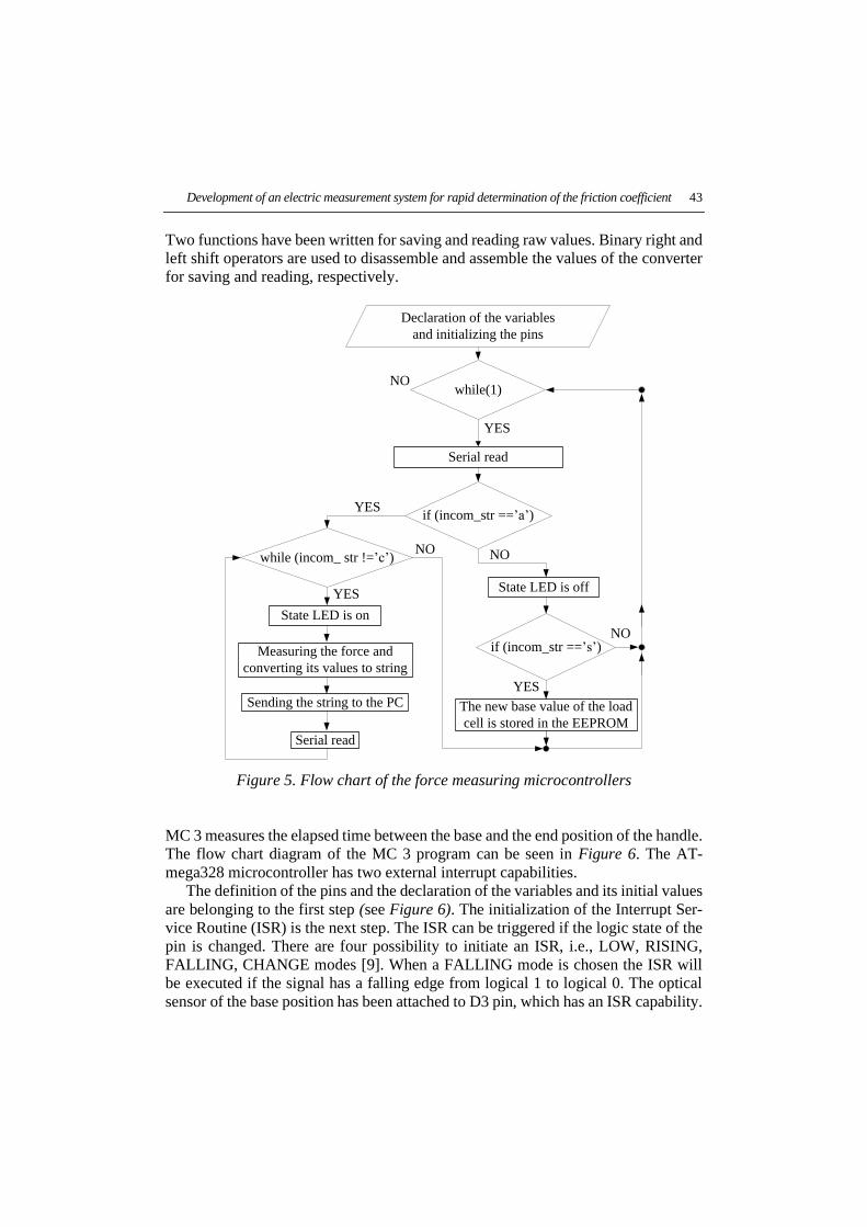
Development of an electric measurement system for rapid determination of the friction coefficient 43
Two functions have been written for saving and reading raw values. Binary right and
left shift operators are used to disassemble and assemble the values of the converter
for saving and reading, respectively.
State LED is on
Sending the string to the PC
Serial read
The new base value of the load
cell is stored in the EEPROM
Declaration of the variables
and initializing the pins
if (incom_str ==’a’)YES
NO
Measuring the force and
converting its values to string
while(1)
Serial read
YES
NO
while (incom_ str !=’c’)
YES
NO
State LED is off
if (incom_str ==’s’)
YES
NO
Figure 5. Flow chart of the force measuring microcontrollers
MC 3 measures the elapsed time between the base and the end position of the handle.
The flow chart diagram of the MC 3 program can be seen in Figure 6. The AT-
mega328 microcontroller has two external interrupt capabilities.
The definition of the pins and the declaration of the variables and its initial values
are belonging to the first step (see Figure 6). The initialization of the Interrupt Ser-
vice Routine (ISR) is the next step. The ISR can be triggered if the logic state of the
pin is changed. There are four possibility to initiate an ISR, i.e., LOW, RISING,
FALLING, CHANGE modes [9]. When a FALLING mode is chosen the ISR will
be executed if the signal has a falling edge from logical 1 to logical 0. The optical
sensor of the base position has been attached to D3 pin, which has an ISR capability.
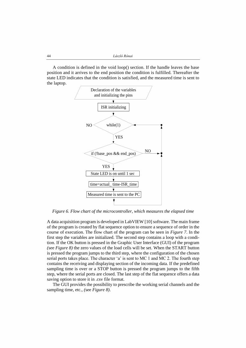
44 László Rónai
A condition is defined in the void loop() section. If the handle leaves the base
position and it arrives to the end position the condition is fulfilled. Thereafter the
state LED indicates that the condition is satisfied, and the measured time is sent to
the laptop.
State LED is on until 1 sec
Declaration of the variables
and initializing the pins
if (!base_pos && end_pos)
YES
while(1)
YES
NO
NO
ISR initializing
Measured time is sent to the PC
time=actual_ time-ISR_time
Figure 6. Flow chart of the microcontroller, which measures the elapsed time
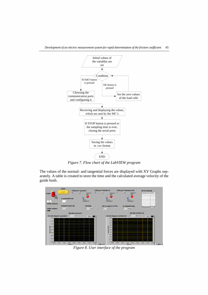
A data acquisition program is developed in LabVIEW [10] software. The main frame
of the program is created by flat sequence option to ensure a sequence of order in the
course of execution. The flow chart of the program can be seen in Figure 7. In the
first step the variables are initialized. The second step contains a loop with a condi-
tion. If the OK button is pressed in the Graphic User Interface (GUI) of the program
(see Figure 8) the zero values of the load cells will be set. When the START button
is pressed the program jumps to the third step, where the configuration of the chosen
serial ports takes place. The character ‘a’ is sent to MC 1 and MC 2. The fourth step
contains the receiving and displaying section of the incoming data. If the predefined
sampling time is over or a STOP button is pressed the program jumps to the fifth
step, where the serial ports are closed. The last step of the flat sequence offers a data
saving option to store it in .csv file format.
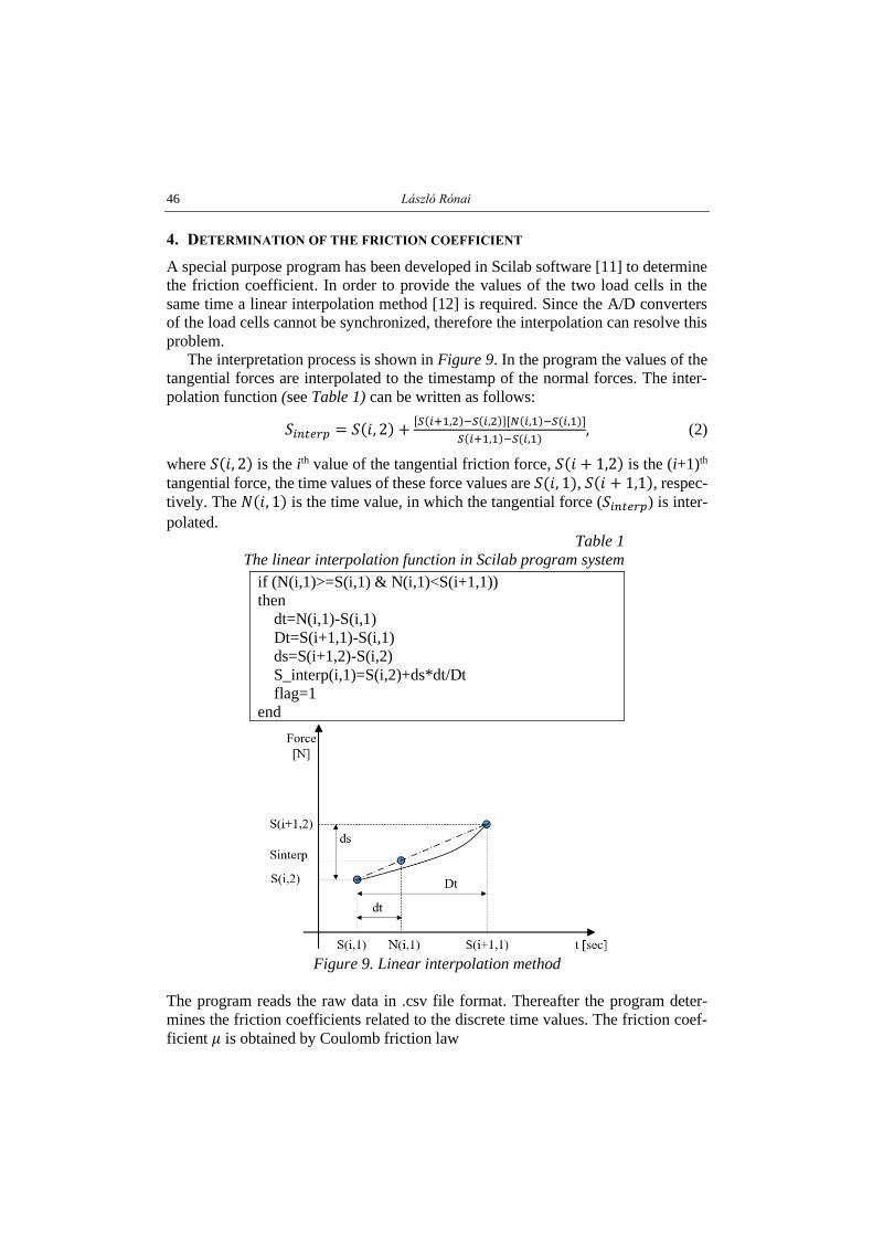
The GUI provides the possibility to prescribe the working serial channels and the
sampling time, etc., (see Figure 8).
Development of an electric measurement system for rapid determination of the friction coefficient 45
Initial values of
the variables are
set
Condition
OK button is
pressed
START button
is pressed
Set the zero values
of the load cells
Choosing the
communication ports
and configuring it
Receiving and displaying the values,
which are sent by the MC’s
If STOP button is pressed or
the sampling time is over,
closing the serial ports
Saving the values
in .csv format
END
Figure 7. Flow chart of the LabVIEW program
The values of the normal- and tangential forces are displayed with XY Graphs sep-
arately. A table is created to store the time and the calculated average velocity of the
guide bush.
Figure 8. User interface of the program
46 László Rónai
4. DETERMINATION OF THE FRICTION COEFFICIENT
A special purpose program has been developed in Scilab software [11] to determine
the friction coefficient. In order to provide the values of the two load cells in the
same time a linear interpolation method [12] is required. Since the A/D converters
of the load cells cannot be synchronized, therefore the interpolation can resolve this
problem.
The interpretation process is shown in Figure 9. In the program the values of the
tangential forces are interpolated to the timestamp of the normal forces. The inter-
polation function (see Table 1) can be written as follows:
𝑆𝑖𝑛𝑡𝑒𝑟𝑝 = 𝑆(𝑖, 2) +[𝑆(𝑖+1,2)−𝑆(𝑖,2)][𝑁(𝑖,1)−𝑆(𝑖,1)]
𝑆(𝑖+1,1)−𝑆(𝑖,1), (2)
where 𝑆(𝑖, 2) is the ith value of the tangential friction force, 𝑆(𝑖 + 1,2) is the (i+1)th
tangential force, the time values of these force values are 𝑆(𝑖, 1), 𝑆(𝑖 + 1,1), respec-
tively. The 𝑁(𝑖, 1) is the time value, in which the tangential force (𝑆𝑖𝑛𝑡𝑒𝑟𝑝) is inter-
polated.
Table 1
The linear interpolation function in Scilab program system
if (N(i,1)>=S(i,1) & N(i,1)<S(i+1,1))
then
dt=N(i,1)-S(i,1)
Dt=S(i+1,1)-S(i,1)
ds=S(i+1,2)-S(i,2)
S_interp(i,1)=S(i,2)+ds*dt/Dt
flag=1
end
Figure 9. Linear interpolation method
The program reads the raw data in .csv file format. Thereafter the program deter-
mines the friction coefficients related to the discrete time values. The friction coef-
ficient 𝜇 is obtained by Coulomb friction law
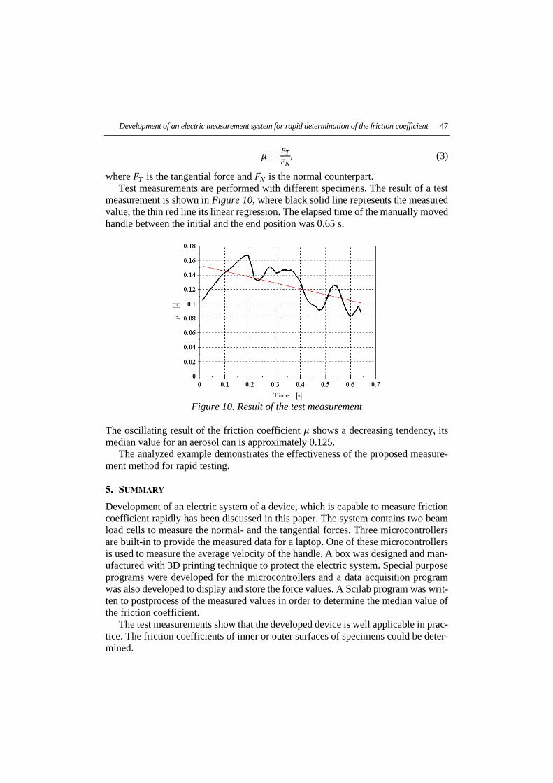
Development of an electric measurement system for rapid determination of the friction coefficient 47
𝜇 =𝐹𝑇
𝐹𝑁, (3)
where 𝐹𝑇 is the tangential force and 𝐹𝑁 is the normal counterpart.
Test measurements are performed with different specimens. The result of a test
measurement is shown in Figure 10, where black solid line represents the measured
value, the thin red line its linear regression. The elapsed time of the manually moved
handle between the initial and the end position was 0.65 s.
Figure 10. Result of the test measurement
The oscillating result of the friction coefficient 𝜇 shows a decreasing tendency, its
median value for an aerosol can is approximately 0.125.
The analyzed example demonstrates the effectiveness of the proposed measure-
ment method for rapid testing.
5. SUMMARY
Development of an electric system of a device, which is capable to measure friction
coefficient rapidly has been discussed in this paper. The system contains two beam
load cells to measure the normal- and the tangential forces. Three microcontrollers
are built-in to provide the measured data for a laptop. One of these microcontrollers
is used to measure the average velocity of the handle. A box was designed and man-
ufactured with 3D printing technique to protect the electric system. Special purpose
programs were developed for the microcontrollers and a data acquisition program
was also developed to display and store the force values. A Scilab program was writ-
ten to postprocess of the measured values in order to determine the median value of
the friction coefficient.
The test measurements show that the developed device is well applicable in prac-
tice. The friction coefficients of inner or outer surfaces of specimens could be deter-
mined.
48 László Rónai
ACKNOWLEDGEMENT
The described article was carried out as part of the EFOP-3.6.1-16-2016-00011
Younger and Renewing University – Innovative Knowledge City – institutional de-
velopment of the University of Miskolc aiming at intelligent specialisation project
implemented in the framework of the Szechenyi 2020 program. The realization of
this project is supported by the European Union, co-financed by the European Social
Fund.
REFERENCES
[1] Andersson S., Söderberg A., Björklund S. (2007). Friction models for sliding
dry, boundary and mixed lubricated contacts. Elsevier Ltd., Tribology Inter-
national, Vol. 40, Issue 4, pp. 580–587.
[2] Liu, Y. F., Zhang, Z. M., Hu, X. H., Zhang, W. J. (2015). Experimental com-
parison of five friction models on the same test-bed of the micro stick-slip
motion system. Mech. Sci., 6, pp. 15–28.
[3] Lorestani, A. N., Rabani, H., Khazaei, Y. (2012). Design and construction of
an automatic coefficient of friction measuring device. Agric. Eng. Int.: CIGR
Journal, Vol. 14, No. 1, pp. 120–124.
[4] Aznar Fernández, Juan Diego (2015). Experimental determination of the fric-
tion coefficient using a tilted plane. pp. 1–5. Doi: 10.13140/RG.2.1.3851.2161.
[5] Hasankhani-Ghavam, F., Abbaspour-Gilandeh, Y., Shahgoli, G., Rahmanza-
deh-Bahram, H. (2015). Design, manufacture and evaluation of the new in-
strument to measure the friction coefficient of soil. Agric. Eng. Int.: CIGR
Journal, Vol. 17, No. 1, pp. 101–109.
[6] Gál, G. (2019). Experimental Determination of the Friction Coefficient.
Study, University of Miskolc (in Hungarian).
[7] Atmel (2009). 8-bit AVR Microcontroller with 4/8/16/32K Bytes In-System
Programmable Flash. Datasheet, Rev. 8025I–AVR–02/09.
[8] AVIA Semiconductor: 24-Bit Analog-to-Digital Converter (ADC) for Weigh
Scales. Datasheet, 2016.
[9] Arduino prototyping platform: https://www.arduino.cc/.
[10] Larsen, R. W. (2011). LabVIEW for Engineers. Prentice Hall, Upper Saddle
River, New Jersey.
[11] The Scilab Consortium: http://www.scilab.org.
[12] Lepot, M., Aubin, J. B., Clemens, F. H. L. R. (2017). Interpolation in Time Se-
ries: An Introductive Overview of Existing Methods. Their Performance Crite-
ria and Uncertainty Assessment. Journal Water, Vol. 9, Issue 10, pp.1–20.
Design of Machines and Structures, Vol. 10, No. 1 (2020), pp. 49–62.
Doi: 10.32972/dms.2020.006
EVOLUTIONARY BASED SYSTEM FOR QUALIFICATION AND
EVALUATION – A CASE STUDY
FERENC JÁNOS SZABÓ
University of Miskolc, Department of Machine and Product Design
3515, Miskolc-Egyetemváros
Abstract: In a previous paper the new EBSYQ (Evolutionary Based SYstem for Qualifica-
tion and Evaluation of Group Achievements) system has been proposed for teachers and ju-
ries, helping them in making accurate and objective ranking. The analysis of the behaviour
of the special characteristic sigmoid functions of the groups gives the possibility to discover
some interesting points of view for qualifying the achievement and the standard of the groups
(subgroups of talented and under- motivated students, spectrum of the group, eigenvalues,
Lorentz function). This paper shows a case study of an international project of student groups
competition in the field of product design, with Finnish and Hungarian students. Comparison
of the decision process of the jury without using the EBSYQ system and with the application
of the system shows the efficiency of the qualification system in realizing a well-founded and
careful ranking of the groups, even in case of very close competition. Each point of view of
the decision-making system is evaluated by numbers, which can increase the objectivity and
accuracy of the decision.
Keywords: Sigmoid functions; evolutionary based system; evaluation, qualification and com-
parison of group achievements; EBSYQ methodology of qualification and evaluation.
1. INTRODUCTION
In this paper a system is shown and applied for evaluation, ranking and comparison
of results and achievements of groups or teams. The proposed system for comparison
and evaluation (EBSYQ) [1] can provide advantages to each participant in engineer-
ing education, testing or competitions: Teachers could more easily find the target
groups for special attention (close- up consultations, coaching, special instructions,
talent treatment etc.), the jury or decision makers could make decisions or selections
more quickly and objectively, eminent students could receive prizes or appropriate
ranking based on objective and accurate decisions, failing student could receive more
appropriate and targeted special consultations.
The efficiency of the proposed system is demonstrated through a case study of an
international project competition (RePCI, Reshaped Partnerships for Competitive-
ness and Innovation Potentials in Mechanical Engineering) of students. The deci-
sion-making process of the jury deciding the winning team of the competition is

50 Ferenc János Szabó
compared when they make the decision without using the EBSYQ system and we
can see the advantages when the system is used.
The case study shows that without the proposed system the results of the groups
are extremely close, if in one criterion one group was better, the other group was
better from an other point of view, so the final decision would normally contain a
high percentage of subjectivity. Since the new system is able to detect and compare
numerically every small differences, this subjectivity can be eliminated and the de-
cisions will be more objective, more precise and based on accurate numerical justi-
fication.
2. CASE STUDY: INTERNATIONAL STUDENT PROJECT ON PRODUCT DEVELOPMENT
Between September 2014 and January 2015, within the framework of the EU-fi-
nanced RePCI [2] (Reshaped Partnerships for Competitiveness and Innovation Po-
tentials in Mechanical Engineering) international project [3], JAMK (Jyväskylä Uni-
versity of Applied Sciences, Finland) and UM (Institute of Machine and Product
Design, University of Miskolc, Hungary) [4] carried out an international student pro-
ject in product development, titled “Design of a multifunctional garden tool” with
the helps and suggestions of the experts of Robert Bosch Power Tool Company,
Miskolc, Hungary.
Each partner university participated with an 8-member team, two teams were
formed, each with 3 Finnish and 5 Hungarian students. The two groups received the
same instructions and the same objective, but after this the groups worked separately,
within competition-like circumstances, without communication between the two
groups, even keeping their results secret from each other.
The objectives of the project were to:
‒ Increase intercultural competence
‒ Solve real-life problems
‒ Make contacts with international companies
‒ Gain interdisciplinary project skills
‒ Obtain deeper knowledge in project management
‒ Communication between group members during project realisation
‒ Increase social competence and communication skills
‒ Improve the ability to work in teams.
The total time of the project was one complete semester and the students worked
in the project as if completing a course, receiving 5 credits at the end. Two inten-
sive weeks were organised: the first intensive week was at the very beginning of
the project, in September 2014, in Miskolc, Hungary, with an introduction section,
and a chance for the Finnish and Hungarian students to get acquainted. During a
visit to the Bosch factory, the students received the description of the task, require-
ments of the product to be designed and all the necessary instructions to start the
project. They selected their own team leader from the members of the team, and
Evolutionary based system for qualification and evaluation – A case study 51
they made every decision concerning the necessary steps of the solution, time
scheduling, task distribution amongst the team members, etc. Two supervisors
(teachers of mechanical engineering, with project realisation experience) visited
both teams regularly to answer questions and give useful instructions during the
solution of the problems.
After the first intensive week the group members continued their work using com-
munication possibilities offered by the Internet (Google, Skype, e-mail, chat, Face-
book etc.). They solved the questions and sub-problems decided and distributed dur-
ing the first intensive week and they exchanged their results. This system was a great
challenge for the team leaders as well, working with groups with members in differ-
ent countries.
The second intensive week was in Jyväskylä, Finland, at the end of October 2014.
After one month of working, during this intensive week they put together their task
results, started to form the main concept of the designed product, and determined the
further steps necessary to solve the task completely. After the intensive week every-
one continued the work, similarly to after the first intensive week.
The project ended with a video-conference day in January 2015, where both
groups presented their results, each student having the chance to present his/her
own results, ideas and solutions in 5–10 minutes. After the presentations they re-
sponded to the questions and comments of supervisors, project manager, or others
in the audience. The work of the students was evaluated by the expert of the Bosch
factory and by the supervisors. Representatives of the local press (TV, radio, news-
papers) reported this event in the news, showing the pictures of the resulting prod-
ucts of the teams, giving a wider platform and reputation to the work and results
of the students.
2.1. Comparison of the groups without the EBSYQ system
At the end of the semester, the project reaching the stage of evaluating, comparing
and ranking the teams and the students participating in the project. Supervisors and
managers of the project and institutions together had to give detailed opinions and
evaluations on the work and results of the groups. Since both of the teams worked
excellently and each had a new and fully elaborated concept of a garden tool as
their result, the jury was really in a difficult position in making the decision of
which group could be the winner. As shown in Table 1, the two groups were very
good and their results were equivalent – if one group was better in one point of
view, other group was better in a different aspect. At that time the system proposed
in this paper was not yet available, therefore the decision at the end was very sub-
jective: Group A was chosen as the winning team, but the close result and out-
standing work of both groups were emphasised. Table 1 shows the points of view
used for the comparison of the groups and the points given (average points given
by the members of the jury).

52 Ferenc János Szabó
Table 1
Comparison of groups without EBSYQ system
(out of five points per item)
Points of view Group
A
Group
B
Communication, interaction, attention to each
other 4 5
Distribution of tasks, organisation of the work 3 4
Time scheduling, creating and meeting
deadlines 5 3
Partitioning the tasks and assigning them
to members 4 4
Forming the main conception of the product 5 4
Price-analysis, material and technology costs 5 4
Taking into account the opinion
of the customers 4 5
Marketing, advertising and communicating
results 5 4
Presentation :
Timing, rhythm, fluency 5 4
Content, quality 4 4
Figures, pictures, colors 4 5
Each member presents his/her results 4 5
Communication with supervisors, questions 4 5
Sum of the points 56 56
2.2. Comparison using the EBSYQ system
For comparison, the usage of the evaluation and comparison system EBSYQ is
demonstrated, following the method of the system, analysing the curves and charac-
teristics of the groups. Since this system needs the point results of the group mem-
bers, it is necessary to create points for the individual comparison of the students and
it is necessary to give the points. This step is the only subjective one in this system.
A short description of the group members, without giving the names or without iden-
tifying the individuals:
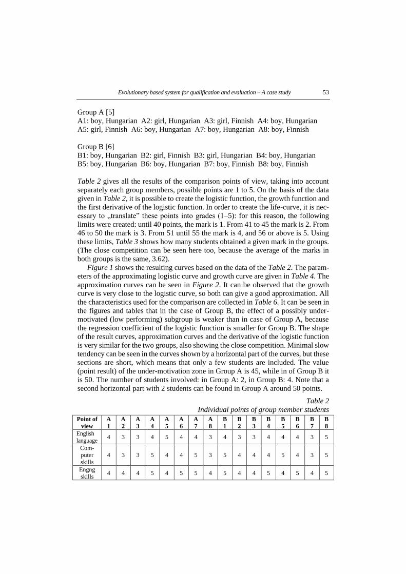
Evolutionary based system for qualification and evaluation – A case study 53
Group A [5]
A1: boy, Hungarian A2: girl, Hungarian A3: girl, Finnish A4: boy, Hungarian
A5: girl, Finnish A6: boy, Hungarian A7: boy, Hungarian A8: boy, Finnish
Group B [6]
B1: boy, Hungarian B2: girl, Finnish B3: girl, Hungarian B4: boy, Hungarian
B5: boy, Hungarian B6: boy, Hungarian B7: boy, Finnish B8: boy, Finnish
Table 2 gives all the results of the comparison points of view, taking into account
separately each group members, possible points are 1 to 5. On the basis of the data
given in Table 2, it is possible to create the logistic function, the growth function and
the first derivative of the logistic function. In order to create the life-curve, it is nec-
essary to „translate” these points into grades (1–5): for this reason, the following
limits were created: until 40 points, the mark is 1. From 41 to 45 the mark is 2. From
46 to 50 the mark is 3. From 51 until 55 the mark is 4, and 56 or above is 5. Using
these limits, Table 3 shows how many students obtained a given mark in the groups.
(The close competition can be seen here too, because the average of the marks in
both groups is the same, 3.62).
Figure 1 shows the resulting curves based on the data of the Table 2. The param-
eters of the approximating logistic curve and growth curve are given in Table 4. The
approximation curves can be seen in Figure 2. It can be observed that the growth
curve is very close to the logistic curve, so both can give a good approximation. All
the characteristics used for the comparison are collected in Table 6. It can be seen in
the figures and tables that in the case of Group B, the effect of a possibly under-
motivated (low performing) subgroup is weaker than in case of Group A, because
the regression coefficient of the logistic function is smaller for Group B. The shape
of the result curves, approximation curves and the derivative of the logistic function
is very similar for the two groups, also showing the close competition. Minimal slow
tendency can be seen in the curves shown by a horizontal part of the curves, but these
sections are short, which means that only a few students are included. The value
(point result) of the under-motivation zone in Group A is 45, while in of Group B it
is 50. The number of students involved: in Group A: 2, in Group B: 4. Note that a
second horizontal part with 2 students can be found in Group A around 50 points.
Table 2
Individual points of group member students
Point of
view
A
1
A
2
A
3
A
4
A
5
A
6
A
7
A
8
B
1
B
2
B
3
B
4
B
5
B
6
B
7
B
8
English
language 4 3 3 4 5 4 4 3 4 3 3 4 4 4 3 5
Com-
puter
skills
4 3 3 5 4 4 5 3 5 4 4 4 5 4 3 5
Engng
skills 4 4 4 5 4 5 5 4 5 4 4 5 4 5 4 5

54 Ferenc János Szabó
Point of
view
A
1
A
2
A
3
A
4
A
5
A
6
A
7
A
8
B
1
B
2
B
3
B
4
B
5
B
6
B
7
B
8
Eco-
nomy
skills
3 4 4 3 5 4 4 3 4 4 3 4 4 3 3 4
Mana-
ger
skills
3 4 3 4 5 3 4 3 4 3 4 4 5 4 4 5
Com-
muni-
cation
4 4 3 4 5 4 5 3 4 4 4 4 5 4 4 5
Inter-
cul-
tural
skills
3 3 3 5 5 4 4 3 4 3 4 5 5 4 4 5
Tole-
rance 4 4 4 5 5 4 4 3 4 3 4 4 5 4 4 4
Integ-
ration 5 4 3 5 5 4 5 3 5 3 4 4 5 4 4 5
Com-
mun.
with
superv
4 4 3 5 5 4 4 3 5 3 4 4 4 5 4 5
Presen-
tation 5 5 4 5 5 4 5 4 5 3 4 4 5 5 4 5
Quality
of
results
4 4 4 5 5 4 5 3 5 3 4 4 5 4 4 5
Team-
member
skills
4 4 3 4 5 4 4 3 4 3 4 4 5 5 4 4
Sum
of
points
51 45 44 59 63 52 58 41 58 43 50 54 49 55 49 62
Table 3
Data for the life curves of the groups
Group points 41–45 46–50 51–55 56–65
A Grade 2 3 4 5
No. of students 3 0 2 3
B Grade 2 3 4 5
No. of students 1 3 2 2
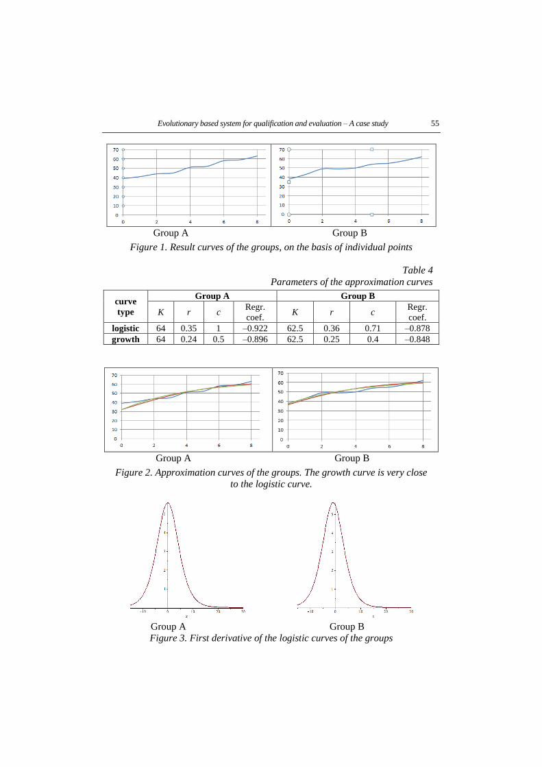
Evolutionary based system for qualification and evaluation – A case study 55
Group A Group B
Figure 1. Result curves of the groups, on the basis of individual points
Table 4
Parameters of the approximation curves
curve
type
Group A Group B
K r c Regr.
coef. K r c
Regr.
coef.
logistic 64 0.35 1 –0.922 62.5 0.36 0.71 –0.878
growth 64 0.24 0.5 –0.896 62.5 0.25 0.4 –0.848
Group A Group B
Figure 2. Approximation curves of the groups. The growth curve is very close
to the logistic curve.
Group A Group B
Figure 3. First derivative of the logistic curves of the groups
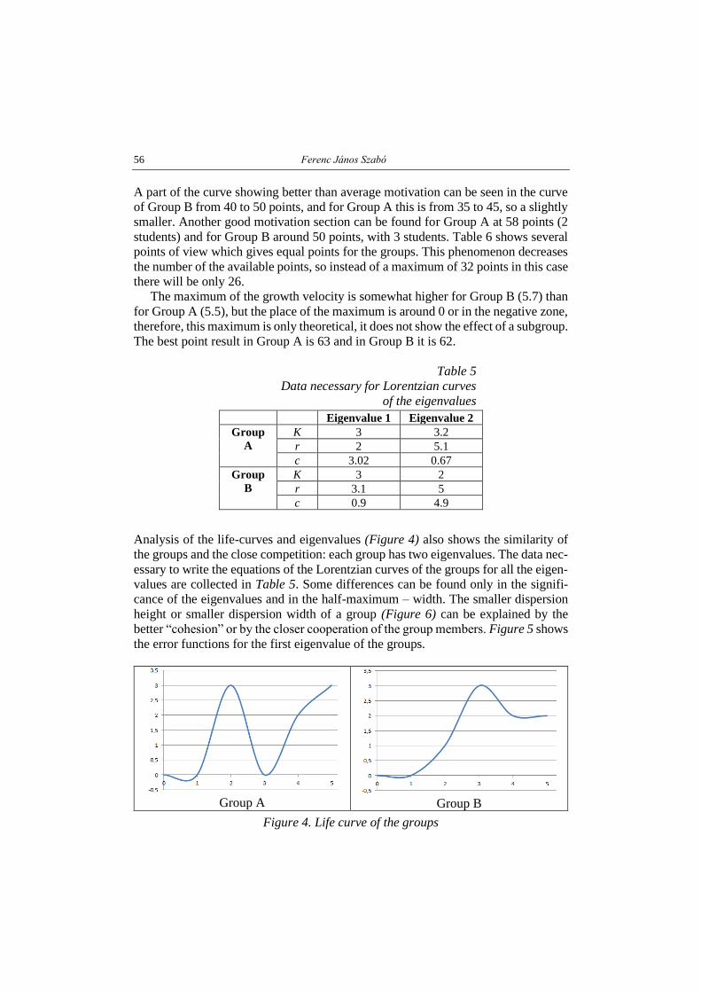
56 Ferenc János Szabó
A part of the curve showing better than average motivation can be seen in the curve
of Group B from 40 to 50 points, and for Group A this is from 35 to 45, so a slightly
smaller. Another good motivation section can be found for Group A at 58 points (2
students) and for Group B around 50 points, with 3 students. Table 6 shows several
points of view which gives equal points for the groups. This phenomenon decreases
the number of the available points, so instead of a maximum of 32 points in this case
there will be only 26.
The maximum of the growth velocity is somewhat higher for Group B (5.7) than
for Group A (5.5), but the place of the maximum is around 0 or in the negative zone,
therefore, this maximum is only theoretical, it does not show the effect of a subgroup.
The best point result in Group A is 63 and in Group B it is 62.
Table 5
Data necessary for Lorentzian curves
of the eigenvalues
Eigenvalue 1 Eigenvalue 2
Group
A
K 3 3.2
r 2 5.1
c 3.02 0.67
Group
B
K 3 2
r 3.1 5
c 0.9 4.9
Analysis of the life-curves and eigenvalues (Figure 4) also shows the similarity of
the groups and the close competition: each group has two eigenvalues. The data nec-
essary to write the equations of the Lorentzian curves of the groups for all the eigen-
values are collected in Table 5. Some differences can be found only in the signifi-
cance of the eigenvalues and in the half-maximum – width. The smaller dispersion
height or smaller dispersion width of a group (Figure 6) can be explained by the
better “cohesion” or by the closer cooperation of the group members. Figure 5 shows
the error functions for the first eigenvalue of the groups.
Group A
Group B
Figure 4. Life curve of the groups

Evolutionary based system for qualification and evaluation – A case study 57
Finally, from the possible 26 points of Table 6, Group A wins 14 and Group B wins
12, so the decision is that Group A will be the winner, with 53.85% of the points
while Group B has 46.15% of the points. (soccer-like result: 7 to 6 for Group A, it
was really a very close fight!).
Table 6
Summarizing table of the characteristics
Type of
curve Parameter name
No-
ta-
tion
Group
A
Group
B Comment Wins
Real
curve of
results
Slow growth
(horizontal) L/H 0.04 0.076 Length/value A
No. of students
involved n 3 4
More motivation
needed A
Average
of point results Pav 3.62 3.62
Easily
comparable –
Growth
function
Regression
coefficient Rkg –0.896 –0.848
Strength
of correlation A
K K 64 62.5 Capacity
of the group A
r r 0.24 0.25 Evolution
(growth) velocity B
c c 0.5 0.4 Parameter
with mixed effect –
Logistic
function
Regression
coefficient Rkl –0.922 –0.877
Strength
of conclusions B
No. of failed
students Am 2 0 Undermotivation B
K K 64 62.5 Capacity
of the group A
r r 0.35 0.36 Growth speed B
c c 1 0.71 Parameter
with mixed effect –
Place of under-
motivation Mh 45 50 Point result B
No. low motiv.
students Msz 2 4 Sub-group A
Excellent value U 63 62 Record, best
result A
No. of excellent
students Usz 1 1
Better
in the group –
Place of higher
motivation Em 58 50 For which result A
No. high motiv.
students Esz 2 3
How many
students B
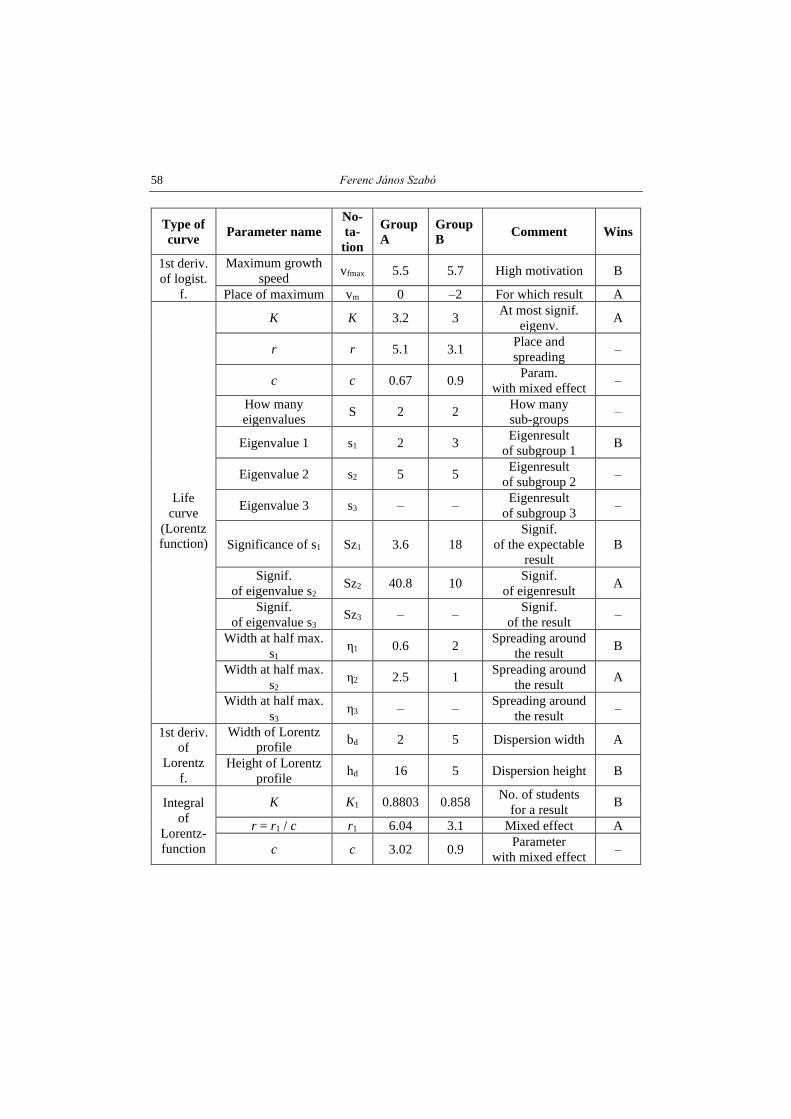
58 Ferenc János Szabó
Type of
curve Parameter name
No-
ta-
tion
Group
A
Group
B Comment Wins
1st deriv.
of logist.
f.
Maximum growth
speed vfmax 5.5 5.7 High motivation B
Place of maximum vm 0 –2 For which result A
Life
curve
(Lorentz
function)
K K 3.2 3 At most signif.
eigenv. A
r r 5.1 3.1 Place and
spreading –
c c 0.67 0.9 Param.
with mixed effect –
How many
eigenvalues S 2 2
How many
sub-groups –
Eigenvalue 1 s1 2 3 Eigenresult
of subgroup 1 B
Eigenvalue 2 s2 5 5 Eigenresult
of subgroup 2 –
Eigenvalue 3 s3 – – Eigenresult
of subgroup 3 –
Significance of s1 Sz1 3.6 18
Signif.
of the expectable
result
B
Signif.
of eigenvalue s2 Sz2 40.8 10
Signif.
of eigenresult A
Signif.
of eigenvalue s3 Sz3 – –
Signif.
of the result –
Width at half max.
s1 η1 0.6 2
Spreading around
the result B
Width at half max.
s2 η2 2.5 1
Spreading around
the result A
Width at half max.
s3 η3 – –
Spreading around
the result –
1st deriv.
of
Lorentz
f.
Width of Lorentz
profile bd 2 5 Dispersion width A
Height of Lorentz
profile hd 16 5 Dispersion height B
Integral
of
Lorentz-
function
K K1 0.8803 0.858 No. of students
for a result B
r = r1 / c r1 6.04 3.1 Mixed effect A
c c 3.02 0.9 Parameter
with mixed effect –
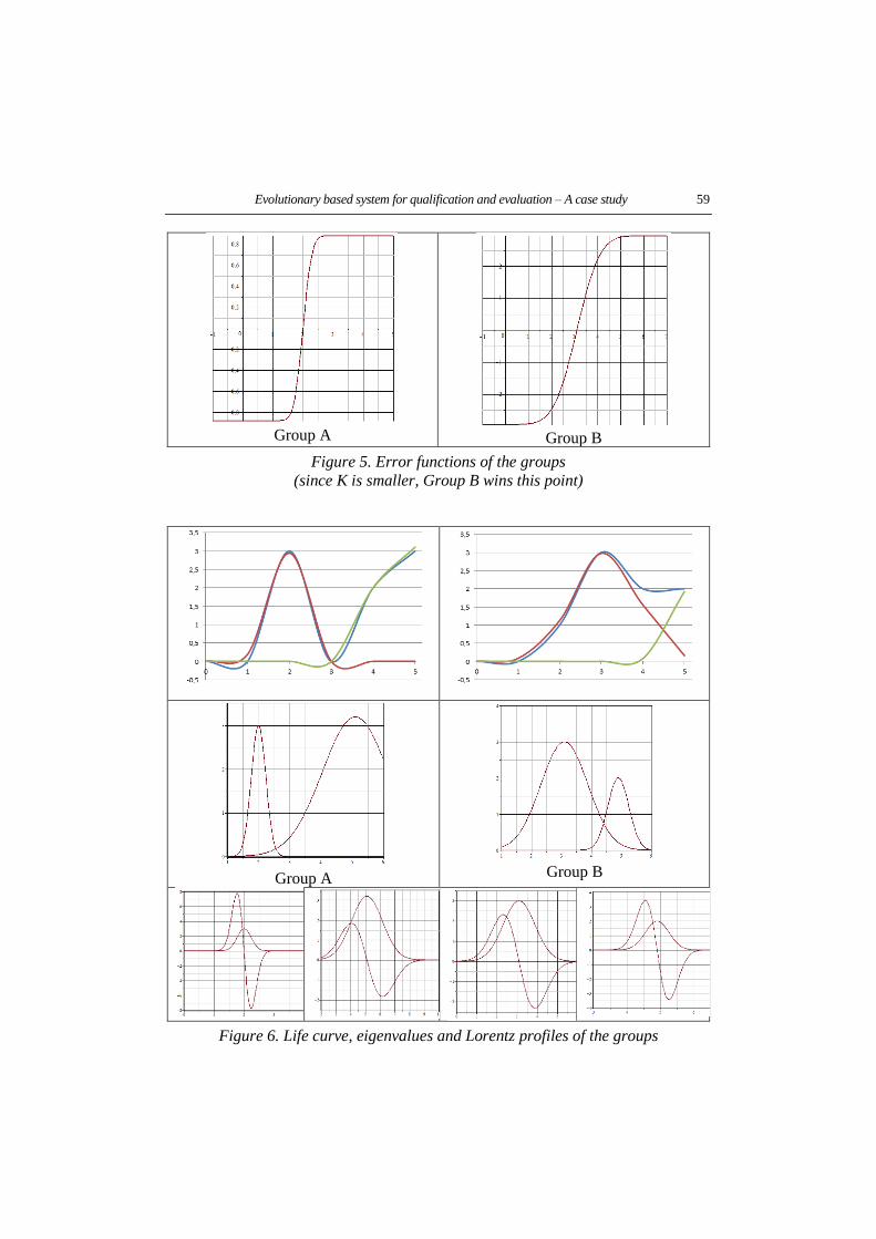
Evolutionary based system for qualification and evaluation – A case study 59
Group A
Group B
Figure 5. Error functions of the groups
(since K is smaller, Group B wins this point)
Group A
Group B
Figure 6. Life curve, eigenvalues and Lorentz profiles of the groups
60 Ferenc János Szabó
Equations of the characteristic curves:
Logistic function: Growth function: Lorentz function:
𝑦(𝑥) =𝐾
1+𝑐𝑒−𝑟𝑥 𝑦(𝑥) = 𝐾(1 − 𝑐𝑒−𝑟𝑥) 𝑦(𝑥) =
𝐾
𝑒𝑐2(𝑥−𝑟)2
The Lorentz profile is the first derivative of the Lorentz function.
3. SUMMARY
In this paper an evolutionary based evaluation and qualification system (EBSYQ) is
proposed and applied for the comparison of group or team results or achievements.
The evolutionary basis of the system comes from the application of sigmoid curves
(growth curve, logistic curve), since these curves can be used also for the description
of the iteration history of evolutionary type optimisation algorithms. Thirty-eight
different points of view are collected for the comparison of the group results, (twelve
of these points of view were equal or impossible to decide the winner of it). On the
basis of these comparison criteria it will be very easy for a teacher to find the appro-
priate target–sub-group for a given type of special work or consultation activity (for
talented students, competitions for outstanding students, increasing the interest and
attendance of average students, or special consultations or remedial work for under-
motivated or failed students). The application of this system during a competition
among groups (or selection of possible applicants for a job, etc.) makes possible to
the decision makers to see the existing differences more clearly, even if they are
small, and hard to detect or notice in other ways. This could help a jury or decision
makers to make decisions in more objective and accurate manner, numerically eval-
uating and comparing each point of view during the comparison process. The work-
ing and efficiency of the proposed system is shown by the comparison of the decision
making process during an international product design cooperation project with the
participation of Finnish and Hungarian student groups as a case study, with and with-
out the proposed system. The case study shows that without the proposed system the
results of the groups are extremely close, if in one criterion one group was better, the
other group was better from an other point of view, so the final decision would nor-
mally contain a high percentage of subjectivity. Analysis of the case study by the
EBSYQ system proves that the proposed method can detect and separate even very
small differences clearly and characterise them numerically, which can be useful
help even in case of very close competitions.
Application of the EBSYQ evaluation system of group achievements can be an
efficient tool in several decision-making situations in scientific and education fields,
resulting more accurate and more objective decisions, which can give advantages to
teachers in finding more precisely the target groups for special treatments and con-
sultations, or to decision makers in making better decisions more easily and quickly,
to the students or to the members of evaluated groups to win and obtain with higher
probability and on more objective basis the prize they are compete for and to arrive
more surely in a position where they can enjoy the results of their long, hard and
Evolutionary based system for qualification and evaluation – A case study 61
diligent work. These results can be also useful during increasing the development
and methodology skills [7] of students and designers, as well as during the design of
talent- treatment, talent- nurturing programmes [8].
Further research in this theme could be to extend this system to other fields of
life: analysis and comparison of sports results (groups, individuals) or analysis of
evolutionary type optimisation algorithms.
ACKNOWLEDGEMENTS
In connection with the case study shown in this paper, the authors would like to say
special thanks to the project RePCI (Reshaped Partnerships for Competitiveness and
Innovation Potentials in Mechanical Engineering), co-financed by EU Lifelong
Learning Program. The research work presented in this paper is partly based on the
results achieved within the following project:
HEIBus 575660-EPP-1-2016-1-FI-EPPKA2-KA (Smart HEI- Business Collabora-
tion for Skills and Competitiveness) ERASMUS+ International Project
(HEI = Higher Education Institutes).
The realization of this project is co-supported by the European Union, co-financed
by the European Social Fund.
REFERENCES
[1] Szabó, F. J. (2017). Evolutionary Based System for Qualification and Evalu-
ation of Group Achievements (EBSYQ). International Journal of Current Re-
search, Vol. 9, Issue 08, pp. 55507–55516, ISSN: 0975-833X, www.jour-
nalcra.com/sites/default/files/21246.pdf
[2] Kakko, A. (2016). Reshaped Partnerships for Competitiveness and Innovation
Potentials in Mechanical Engineering (RePCI). 44th SEFI (European Society
of Engineering Education) Conference, Tampere, Finland.
[3] Firescu, V., Lapusan,C., Mandru, D., Aksovaara, S. (2015). New Approaches
to Increase Organisational Competitiveness Using Competence Coaching
Concept. Review of Management and Economic Engineering, Vol. 14, No. 2,
pp. 273-278, http://www.mee.org/56engleza.htm
[4] Bognár, G. (2015). Reshaped Partnership and Good Practice in Engineering
Education. 18th International Conference on Interactive Collaborative Learn-
ing (ICL), IEEE Conference Publications, Florence, Italy. pp. 957–963, doi:
10.1109/ICL.2015.7318157.
[5] Birta, T., Herbst, D., Kiss, G., Kivihalme, K., Kublik, B., Mezei, M., Oinonen,
K., Parkkonen, P. (2015). Morphy – the Multifinctional Cordless Garden tool.
(Product Design Project). Design of Machines and Structures, Vol. 5, No.1.
pp. 5–14.

62 Ferenc János Szabó
[6] Nagy, G., Spisák, B., Szója, A., Szántai, I., Jalkanen, J., Mattila, J., Rentola,
M., Puskás, T. (2015). Branch Shaker Designing Project. Design of Machines
and Structures, Vol. 5, No. 2, pp. 17–29.
[7] Kamondi, L., Sarka, F., Takács, Á. (2011). Fejlesztés-módszertani ismeretek
[Development-Methodology Skills] (in Hungarian). Electronic textbook for
students, TÁMOP-4.1.2-08/1/a-2009-0001, Miskolc.
[8] Bérczes, R. (2015). The Improvement of Higher Education Quality and Tal-
ent-nurturing with Scientific Students’ Association (SSA) Commitment. Acta
Polytechnica Hungarica, Vol. 12, No. 5, pp. 101–120.

REVIEWING COMMITTEE
Á. DOBOSY Institute of Materials Science and Technology
University of Miskolc
H-3515 Miskolc-Egyetemváros, Hungary
M. GÁSPÁR Institute of Materials Science and Technology
University of Miskolc
H-3515 Miskolc-Egyetemváros, Hungary
GY. HEGEDŰS Institute of Machine Tools and Mechatronics
University of Miskolc
H-3515 Miskolc-Egyetemváros, Hungary
ZS. KONCSIK Institute of Materials Science and Technology
University of Miskolc
H-3515 Miskolc-Egyetemváros, Hungary
L. RÓNAI Institute of Machine Tools and Mechatronics
University of Miskolc
H-3515 Miskolc-Egyetemváros, Hungary
F. SARKA Institute of Machine and Product Design
University of Miskolc
H-3515 Miskolc-Egyetemváros, Hungary
T. SZABÓ Institute of Machine Tools and Mechatronics
University of Miskolc
H-3515 Miskolc-Egyetemváros, Hungary
Á. TAKÁCS Institute of Machine and Product Design
University of Miskolc
H-3515 Miskolc-Egyetemváros, Hungary
Á. TÖRÖK KTI – Institute for Transport Sciences
H-1119 Budapest,
Than Karoly street 3–5, Hungary

Secreteriat of the Vice-Rector for Research and International Relations,
University of Miskolc,
Responsible for the Publication: Prof. dr. Tamás Kékesi
Published by the Miskolc University Press under leadership of Attila Szendi
Responsible for duplication: Erzsébet Pásztor
Editor: Dr. Ágnes Takács
Technical editor, proofreader: Csilla Gramantik
Number of copies printed: 50
Put the Press in 2020
Number of permission: TNRT–2020– 100 –ME
HU ISSN 1785-6892 in print
HU ISSN 2064-7522 online


![Arya, Suresh - Design of Structures and Foundations for Vibrating Machines [1984].pdf](https://img.pdfslide.net/doc/110x75/55cf9d1d550346d033ac4dce/arya-suresh-design-of-structures-and-foundations-for-vibrating-machines.jpg)