Embed Size (px)
Citation preview
Forward and Inverse Kinematics of Serial Manipulators
RoboticsForward and Inverse Kinematics of Serial Manipulators
Vladimír Smutný
Center for Machine Perception
Czech Institute for Informatics, Robotics, and Cybernetics (CIIRC)
Czech Technical University in Prague
1 23 45 67 89 1011 1213 1415 1617 1819 2021 2223 2425 2627 2829
ROBOTICS: Vladimır Smutny Slide 1, Page 1
Direct and inverse kinematics
Robot usually directly measures its inner kinematic parameters - joint coordinates.Those coordinates measure the position of joints. We denote them usually as ~q, jointcoordinate of the revolute joint is denoted as θ, joint coordinate of the prismatic jointis denoted as d.
User is interested in the position of the end effector or the position of themanipulated rigid body. It has 6 DOF and it could be described in number of ways,e.g. by the transformation matrix describing position of the end effector coordinatesystem in the world coordinate system.
We are interested in the mapping between those two descriptions of the robotposition.
1 23 45 67 89 1011 1213 1415 1617 1819 2021 2223 2425 2627 2829
Students often confuse position of the end effector (6DOF) with the position of the center of the gripper (point- has 3 DOF). This is a crucial error as orientation of the
gripper is important for both manipulation or operation (e.g.welding).
ROBOTICS: Vladimır Smutny Slide 2, Page 2
Direct kinematics
Direct (forward) kinematics is a mapping from joint coordinate space to space ofend-effector positions. That is we know the position of all (or some) individual jointsand we are looking for the position of the end effector. Mathematically:
~q → T(~q)
Direct kinematics could be immediately used in coordinate measurement systems.Sensors in the joints will inform us about the relative position of the links, jointcoordinates. The goal is to calculate the position of the reference point of themeasuring system.
1 23 45 67 89 1011 1213 1415 1617 1819 2021 2223 2425 2627 2829
Let us emphasize, that direct kinematics is mapping, nota mathematical function. It could have none, one, several, or
infinitely many solutions for particular ~q.
ROBOTICS: Vladimır Smutny Slide 3, Page 3
Inverse kinematics
Inverse kinematics is a mapping from space of end-effector positions to jointcoordinate space . That is we know the position of the end effector and we arelooking for the coordinates of all individual joints. Mathematically:
T→ ~q(T)
Inverse kinematics is needed in robot control, one knows the required position of thegripper, but for control the joint coordinates are needed.
1 23 45 67 89 1011 1213 1415 1617 1819 2021 2223 2425 2627 2829
Let us emphasize, that inverse kinematics is mapping, nota mathematical function. It could have none, one, several, or
infinitely many solutions for particular ~q.
ROBOTICS: Vladimır Smutny Slide 4, Page 4
Open kinematic chain
1 23 45 67 89 1011 1213 1415 1617 1819 2021 2223 2425 2627 2829
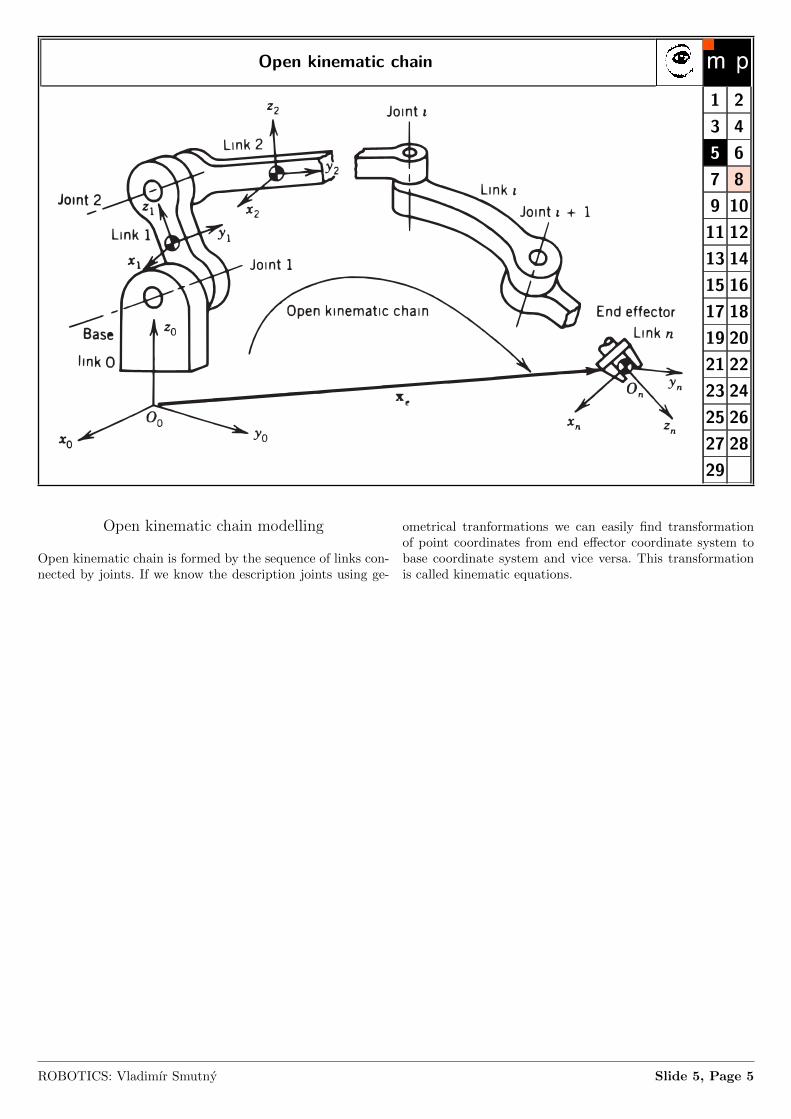
Open kinematic chain modelling
Open kinematic chain is formed by the sequence of links con-nected by joints. If we know the description joints using ge-
ometrical tranformations we can easily find transformationof point coordinates from end effector coordinate system tobase coordinate system and vice versa. This transformationis called kinematic equations.
ROBOTICS: Vladimır Smutny Slide 5, Page 5
Open kinematic chain modeling in plane
y1
x1
y3x3y2
x2
y5
x5
y4
x4
y0
x0
y6
x6
l1
d2
l3
θ1
α2
θ3
φ
1 23 45 67 89 1011 1213 1415 1617 1819 2021 2223 2425 2627 2829
Homogeneous coordinate system transformation could bedescribed by transformation matrix A
x = Axb,
A =
[R xo
0 0 1
]=
cos(φ) − sin(φ) xosin(φ) cos(φ) yo
0 0 1
,where φ is relative rotation of second coordinate system tofirst coordinate system. Inverse matrix is immediately:
A−1 =
[RT −RTxo
0 0 1
]= (1)
=
cos(φ) sin(φ) − cos(φ)xo − sin(φ)yo− sin(φ) cos(φ) sin(φ)xo − cos(φ)yo
0 0 1
, (2)
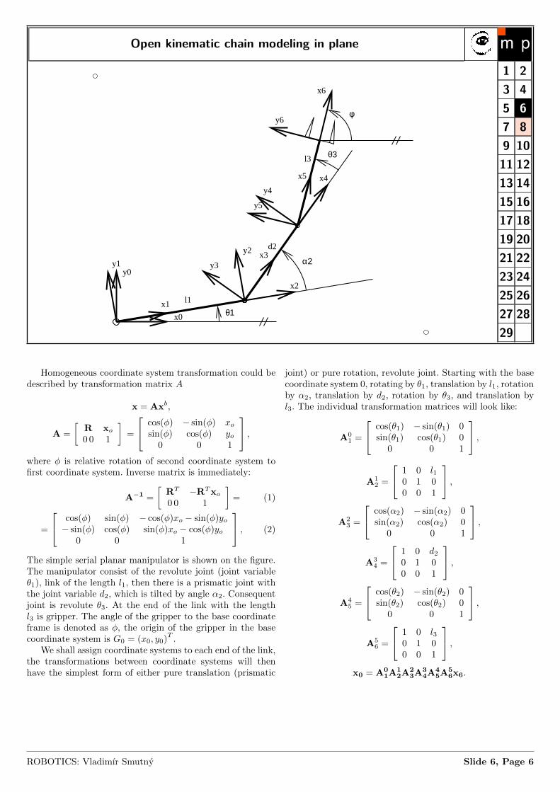
The simple serial planar manipulator is shown on the figure.The manipulator consist of the revolute joint (joint variableθ1), link of the length l1, then there is a prismatic joint withthe joint variable d2, which is tilted by angle α2. Consequentjoint is revolute θ3. At the end of the link with the lengthl3 is gripper. The angle of the gripper to the base coordinateframe is denoted as φ, the origin of the gripper in the basecoordinate system is G0 = (x0, y0)
T.
We shall assign coordinate systems to each end of the link,the transformations between coordinate systems will thenhave the simplest form of either pure translation (prismatic
joint) or pure rotation, revolute joint. Starting with the basecoordinate system 0, rotating by θ1, translation by l1, rotationby α2, translation by d2, rotation by θ3, and translation byl3. The individual transformation matrices will look like:
A01 =
cos(θ1) − sin(θ1) 0sin(θ1) cos(θ1) 0
0 0 1
,
A12 =
1 0 l10 1 00 0 1
,A2
3 =
cos(α2) − sin(α2) 0sin(α2) cos(α2) 0
0 0 1
,A3
4 =
1 0 d20 1 00 0 1
,A4
5 =
cos(θ2) − sin(θ2) 0sin(θ2) cos(θ2) 0
0 0 1
,A5
6 =
1 0 l30 1 00 0 1
,x0 = A0
1A12A
23A
34A
45A
56x6.
ROBOTICS: Vladimır Smutny Slide 6, Page 6
Geometry Intermezzo: Relative Position of Two Straight Lines andTransversal
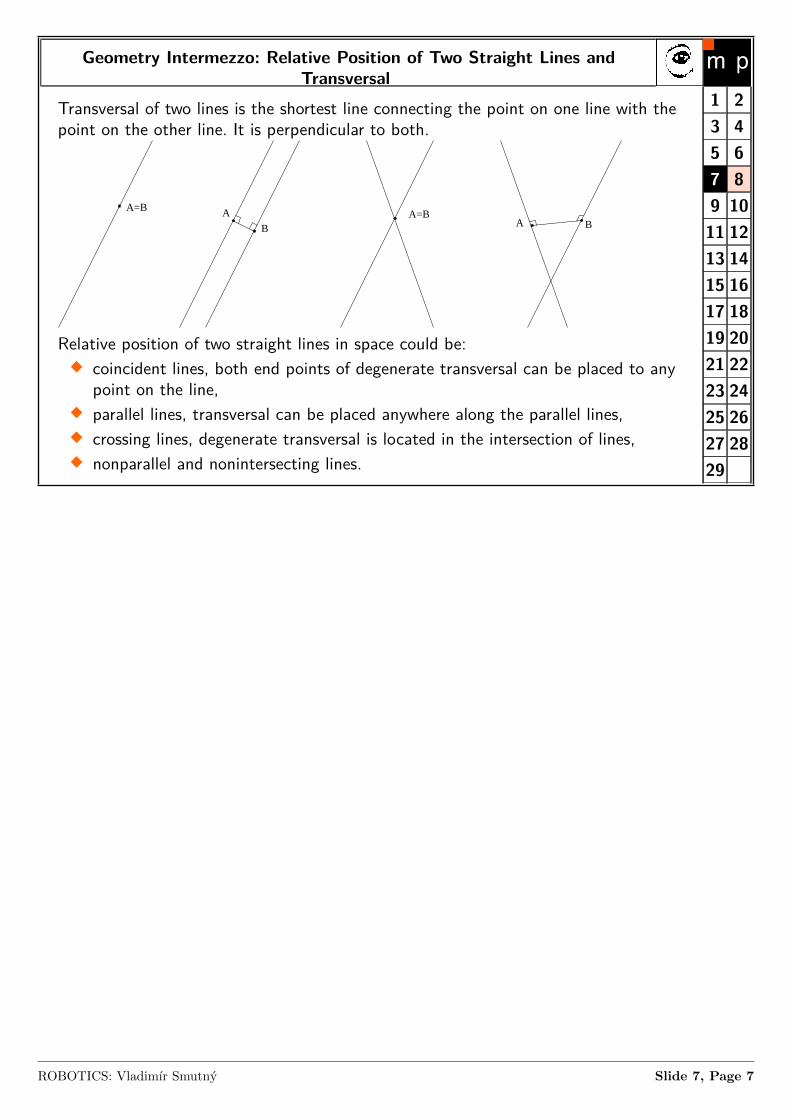
Transversal of two lines is the shortest line connecting the point on one line with thepoint on the other line. It is perpendicular to both.
A=B A
BA=B
A B
Relative position of two straight lines in space could be:� coincident lines, both end points of degenerate transversal can be placed to anypoint on the line,
� parallel lines, transversal can be placed anywhere along the parallel lines,� crossing lines, degenerate transversal is located in the intersection of lines,� nonparallel and nonintersecting lines.
1 23 45 67 89 1011 1213 1415 1617 1819 2021 2223 2425 2627 2829
ROBOTICS: Vladimır Smutny Slide 7, Page 7
Open kinematic chain modeling in space – the Denavit-Hartenbergnotation
1 23 45 67 89 1011 1213 1415 1617 1819 2021 2223 2425 2627 2829
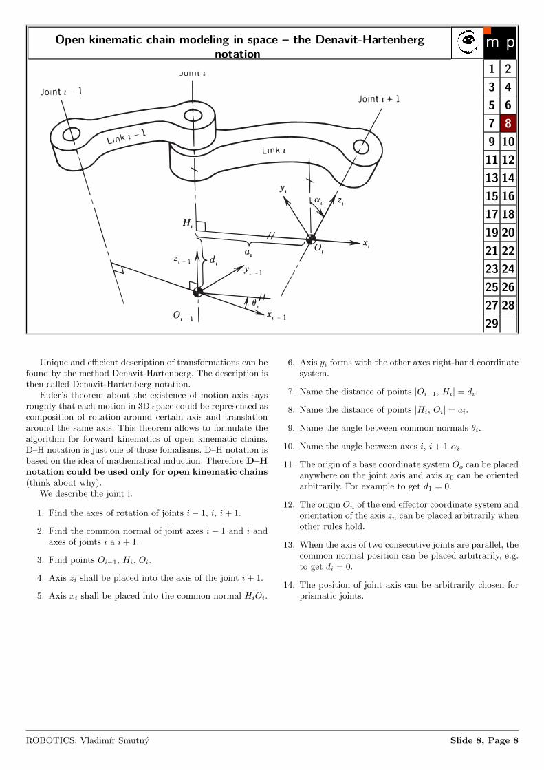
Unique and efficient description of transformations can befound by the method Denavit-Hartenberg. The description isthen called Denavit-Hartenberg notation.
Euler’s theorem about the existence of motion axis saysroughly that each motion in 3D space could be represented ascomposition of rotation around certain axis and translationaround the same axis. This theorem allows to formulate thealgorithm for forward kinematics of open kinematic chains.D–H notation is just one of those fomalisms. D–H notation isbased on the idea of mathematical induction. Therefore D–Hnotation could be used only for open kinematic chains(think about why).
We describe the joint i.
1. Find the axes of rotation of joints i− 1, i, i+ 1.
2. Find the common normal of joint axes i − 1 and i andaxes of joints i a i+ 1.
3. Find points Oi−1, Hi, Oi.
4. Axis zi shall be placed into the axis of the joint i+ 1.
5. Axis xi shall be placed into the common normal HiOi.
6. Axis yi forms with the other axes right-hand coordinatesystem.
7. Name the distance of points |Oi−1, Hi| = di.
8. Name the distance of points |Hi, Oi| = ai.
9. Name the angle between common normals θi.
10. Name the angle between axes i, i+ 1 αi.
11. The origin of a base coordinate system Oo can be placedanywhere on the joint axis and axis x0 can be orientedarbitrarily. For example to get d1 = 0.
12. The origin On of the end effector coordinate system andorientation of the axis zn can be placed arbitrarily whenother rules hold.
13. When the axis of two consecutive joints are parallel, thecommon normal position can be placed arbitrarily, e.g.to get di = 0.
14. The position of joint axis can be arbitrarily chosen forprismatic joints.
ROBOTICS: Vladimır Smutny Slide 8, Page 8
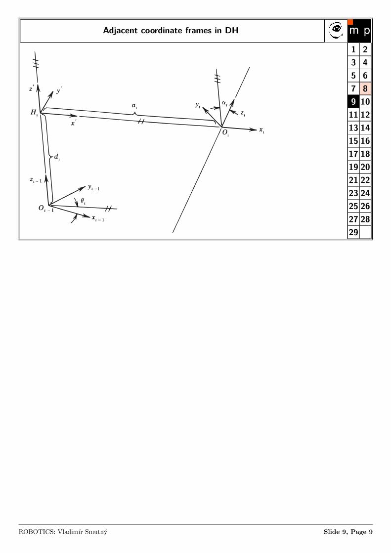
Adjacent coordinate frames in DH
1 23 45 67 89 1011 1213 1415 1617 1819 2021 2223 2425 2627 2829
ROBOTICS: Vladimır Smutny Slide 9, Page 9
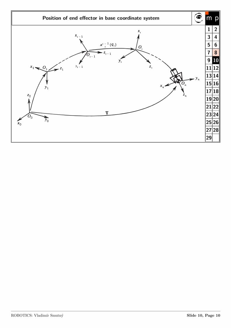
Position of end effector in base coordinate system
1 23 45 67 89 1011 1213 1415 1617 1819 2021 2223 2425 2627 2829
ROBOTICS: Vladimır Smutny Slide 10, Page 10
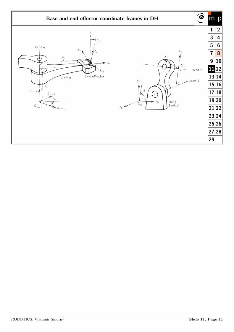
Base and end effector coordinate frames in DH
− −
−−
1 23 45 67 89 1011 1213 1415 1617 1819 2021 2223 2425 2627 2829
ROBOTICS: Vladimır Smutny Slide 11, Page 11
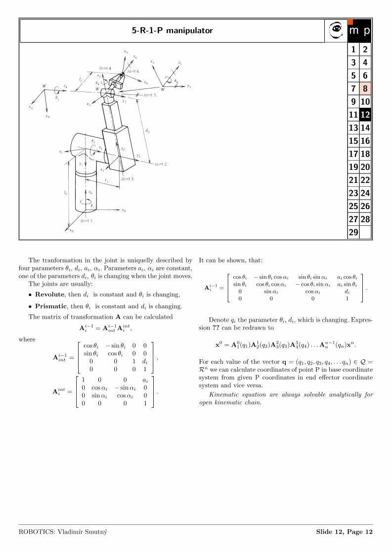
5-R-1-P manipulator
1 23 45 67 89 1011 1213 1415 1617 1819 2021 2223 2425 2627 2829
The tranformation in the joint is uniquelly described byfour parameters θi, di, ai, αi. Parameters ai, αi are constant,one of the parameters di, θi is changing when the joint moves.
The joints are usually:
• Revolute, then di is constant and θi is changing,
• Prismatic, then θi is constant and di is changing.
The matrix of transformation A can be calculated
Ai−1i = Ai−1
int Ainti ,
where
Ai−1int =
cos θi − sin θi 0 0sin θi cos θi 0 0
0 0 1 di0 0 0 1
,
Ainti =
1 0 0 ai0 cosαi − sinαi 00 sinαi cosαi 00 0 0 1
.
It can be shown, that:
Ai−1i =
cos θi − sin θi cosαi sin θi sinαi ai cos θisin θi cos θi cosαi − cos θi sinαi ai sin θi0 sinαi cosαi di0 0 0 1
.
Denote qi the parameter θi, di, which is changing. Expres-sion ?? can be redrawn to
x0 = A01(q1)A1
2(q2)A23(q3)A3
4(q4) . . .An−1n (qn)xn.
For each value of the vector q = (q1, q2, q3, q4, . . . qn) ∈ Q =Rn we can calculate coordinates of point P in base coordinatesystem from given P coordinates in end effector coordinatesystem and vice versa.
Kinematic equation are always solvable analytically foropen kinematic chain.
ROBOTICS: Vladimır Smutny Slide 12, Page 12
Denavit–Hartenberg
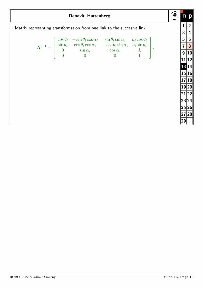
Matrix representing transformation from one link to the succesive link
Ai−1i =
cos θi − sin θi cosαi sin θi sinαi ai cos θi
sin θi cos θi cosαi − cos θi sinαi ai sin θi
0 sinαi cosαi di
0 0 0 1
.
1 23 45 67 89 1011 1213 1415 1617 1819 2021 2223 2425 2627 2829
ROBOTICS: Vladimır Smutny Slide 13, Page 13
Inverse kinematics of 5-R-1-P manipulator
...
−
...
1 23 45 67 89 1011 1213 1415 1617 1819 2021 2223 2425 2627 2829
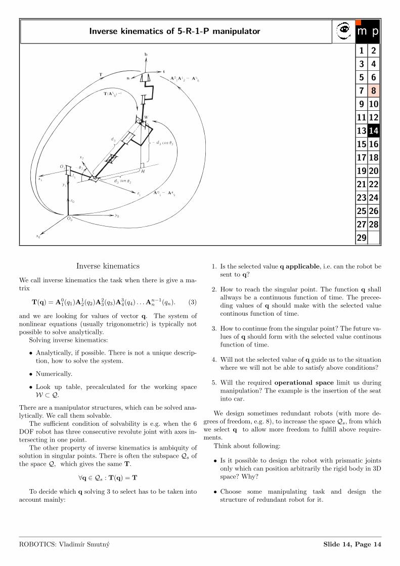
Inverse kinematics
We call inverse kinematics the task when there is give a ma-trix
T(q) = A01(q1)A1
2(q2)A23(q3)A3
4(q4) . . .An−1n (qn). (3)
and we are looking for values of vector q. The system ofnonlinear equations (usually trigonometric) is typically notpossible to solve analytically.
Solving inverse kinematics:
• Analytically, if possible. There is not a unique descrip-tion, how to solve the system.
• Numerically.
• Look up table, precalculated for the working spaceW ⊂ Q.
There are a manipulator structures, which can be solved ana-lytically. We call them solvable.
The sufficient condition of solvability is e.g. when the 6DOF robot has three consecutive revolute joint with axes in-tersecting in one point.
The other property of inverse kinematics is ambiquity ofsolution in singular points. There is often the subspace Qs ofthe space Q, which gives the same T.
∀q ∈ Qs : T(q) = T
To decide which q solving 3 to select has to be taken intoaccount mainly:
1. Is the selected value q applicable, i.e. can the robot besent to q?
2. How to reach the singular point. The function q shallallways be a continuous function of time. The precee-ding values of q should make with the selected valuecontinous function of time.
3. How to continue from the singular point? The future va-lues of q should form with the selected value continousfunction of time.
4. Will not the selected value of q guide us to the situationwhere we will not be able to satisfy above conditions?
5. Will the required operational space limit us duringmanipulation? The example is the insertion of the seatinto car.
We design sometimes redundant robots (with more de-grees of freedom, e.g. 8), to increase the space Qs, from whichwe select q to allow more freedom to fulfill above require-ments.
Think about following:
• Is it possible to design the robot with prismatic jointsonly which can position arbitrarily the rigid body in 3Dspace? Why?
• Choose some manipulating task and design thestructure of redundant robot for it.
ROBOTICS: Vladimır Smutny Slide 14, Page 14
Inverse Kinematics - example
1 23 45 67 89 1011 1213 1415 1617 1819 2021 2223 2425 2627 2829
ROBOTICS: Vladimır Smutny Slide 15, Page 15
Inverse Kinematics - example
2 Robot arm
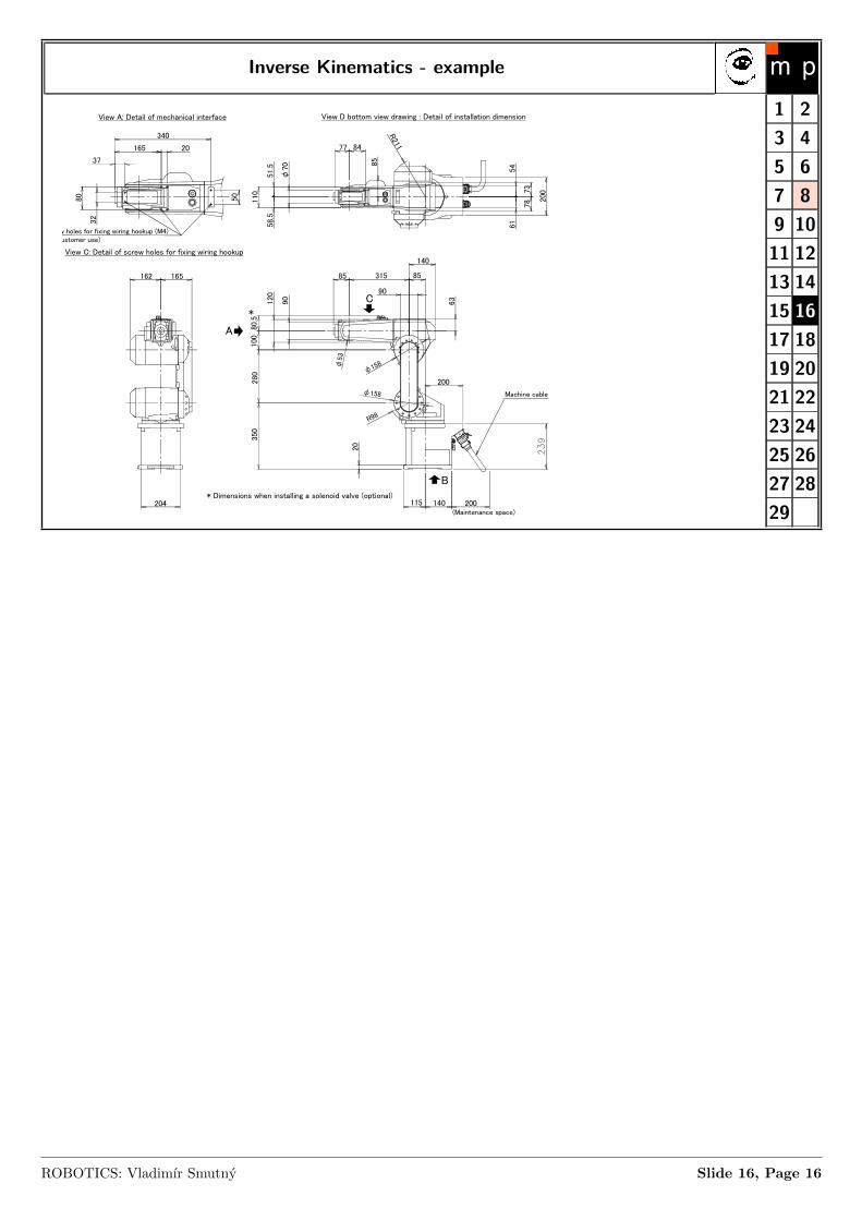
Outside dimensions ・ Operating range diagram 2-13
2.4 Outside dimensions ・ Operating range diagram
(1) RV-6S/6SC
Fig.2-4 : Outside dimensions : RV-6S/6SC
115
96
122
204
160
102.5
205
115 140
4-φ9 installation hole 2-φ6 holes (prepared holes for φ8 positioning pins)
View D bottom view drawing : Detail of installation dimension
6.3a (Installation)
6.3a
(In
stal
lation)
φ31.5
45°
φ20H7+0.0210 depth 7.5
φ40h8 -0.0390 depth 7.5
φ5H7 +0.0120 depth 5
View A: Detail of mechanical interface
4-M5 screw, depth 9
110
R211
51.
558.
5
φ70
77 84
85
5461
7873
200
80
37
32
340
20165
50(for customer use)
View C: Detail of screw holes for fixing wiring hookup
Screw holes for fixing wiring hookup (M4)
162 165
204
A
B
200115 140
φ158
φ158
R98
80.5
100
280
350
120
90
φ53
20
85 85315
140
90
63
200
* Dimensions when installing a solenoid valve (optional)
*
C
(Maintenance space)
Machine cable
1 23 45 67 89 1011 1213 1415 1617 1819 2021 2223 2425 2627 2829
ROBOTICS: Vladimır Smutny Slide 16, Page 16
Inverse Kinematics - example
2-14 Outside dimensions ・ Operating range diagram
2 Robot arm
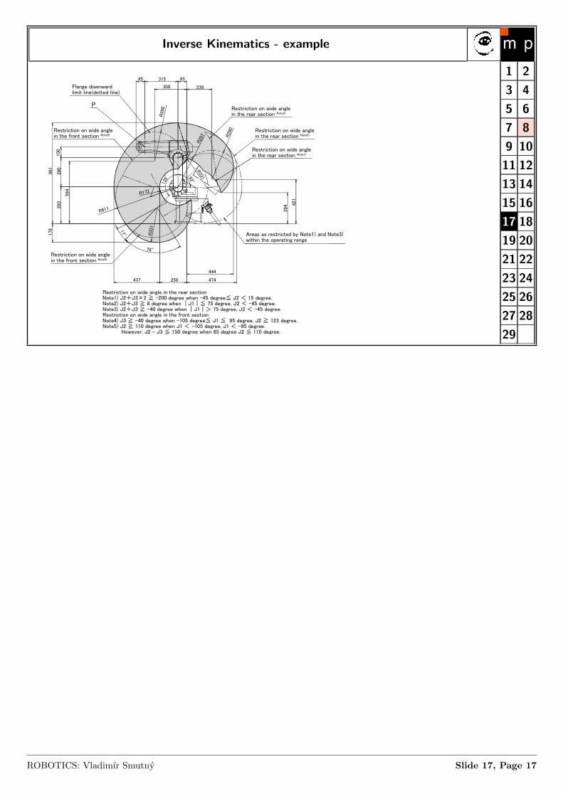
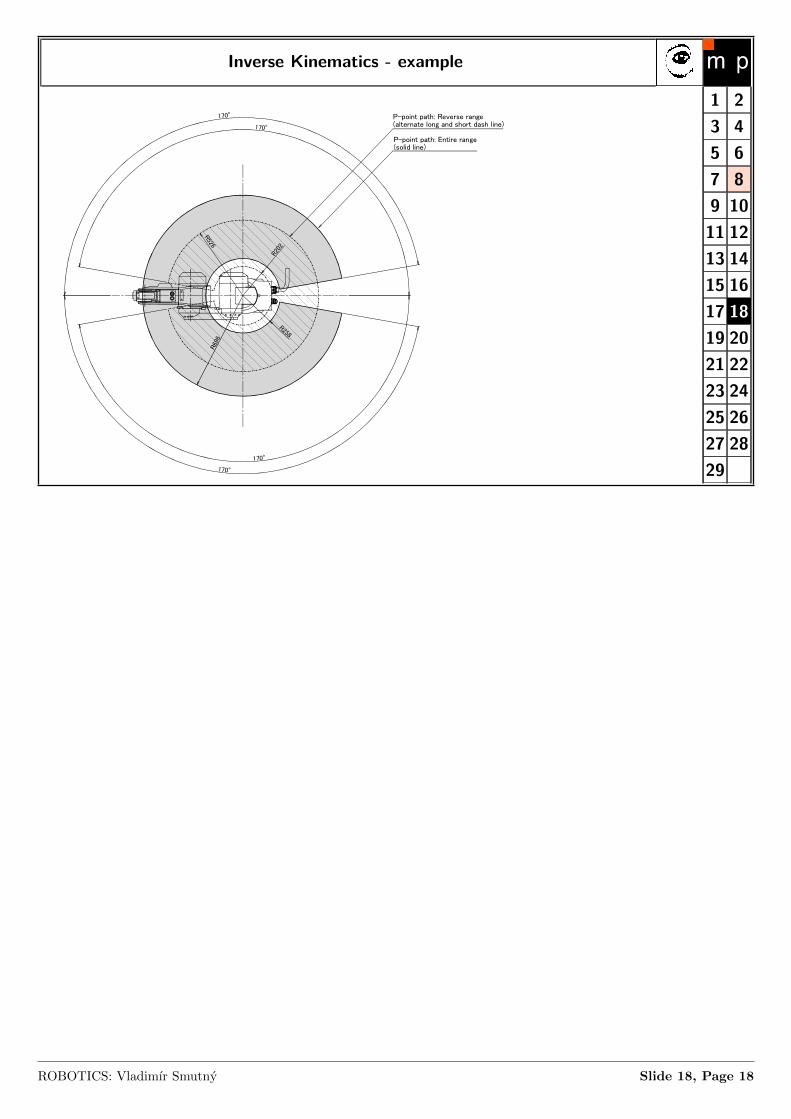
Fig.2-5 : Operating range diagram : RV-6S/6SC
Restriction on wide angle in the rear sectionNote1) J2+J3×2 ≧ -200 degree when -45 degree≦ J2 < 15 degree. Note2) J2+J3 ≧ 8 degree when |J1|≦ 75 degree, J2 < -45 degree. Note3) J2+J3 ≧ -40 degree when |J1|> 75 degree, J2 < -45 degree. Restriction on wide angle in the front sectionNote4) J3 ≧ -40 degree when -105 degree≦ J1 ≦ 95 degree, J2 ≧ 123 degree. Note5) J2 ≧ 110 degree when J1 < -105 degree, J1 < -95 degree. However, J2 - J3 ≦ 150 degree when 85 degree J2 ≦ 110 degree.
170°
170°
170°
R258
R526
R202
R69
6
170°
P-point path: Reverse range (alternate long and short dash line)
P-point path: Entire range (solid line)
P
R611
100
961
280
350
179
85 315
308 238
85
R28
0
R28
0
R173
135°
R33192°
R33
1
76°
17°
R28
7
258437
444
421
294
474
Flange downward limit line(dotted line)
Restriction on wide angle in the rear section Note1)
Areas as restricted by Note1) and Note3) within the operating range
Restriction on wide angle in the rear section Note3)
Restriction on wide angle in the rear section Note2)
Restriction on wide angle in the front section Note5)
Restriction on wide angle in the front section Note4)
594
1 23 45 67 89 1011 1213 1415 1617 1819 2021 2223 2425 2627 2829
ROBOTICS: Vladimır Smutny Slide 17, Page 17
Inverse Kinematics - example
2-14 Outside dimensions ・ Operating range diagram
2 Robot arm
Fig.2-5 : Operating range diagram : RV-6S/6SC
Restriction on wide angle in the rear sectionNote1) J2+J3×2 ≧ -200 degree when -45 degree≦ J2 < 15 degree. Note2) J2+J3 ≧ 8 degree when |J1|≦ 75 degree, J2 < -45 degree. Note3) J2+J3 ≧ -40 degree when |J1|> 75 degree, J2 < -45 degree. Restriction on wide angle in the front sectionNote4) J3 ≧ -40 degree when -105 degree≦ J1 ≦ 95 degree, J2 ≧ 123 degree. Note5) J2 ≧ 110 degree when J1 < -105 degree, J1 < -95 degree. However, J2 - J3 ≦ 150 degree when 85 degree J2 ≦ 110 degree.
170°
170°
170°
R258
R526
R202
R69
6
170°
P-point path: Reverse range (alternate long and short dash line)
P-point path: Entire range (solid line)
P
R611
100
961
280
350
179
85 315
308 238
85
R28
0
R28
0
R173
135°
R33192°
R33
1
76°
17°
R28
7
258437
444
421
294
474
Flange downward limit line(dotted line)
Restriction on wide angle in the rear section Note1)
Areas as restricted by Note1) and Note3) within the operating range
Restriction on wide angle in the rear section Note3)
Restriction on wide angle in the rear section Note2)
Restriction on wide angle in the front section Note5)
Restriction on wide angle in the front section Note4)
594
1 23 45 67 89 1011 1213 1415 1617 1819 2021 2223 2425 2627 2829
ROBOTICS: Vladimır Smutny Slide 18, Page 18
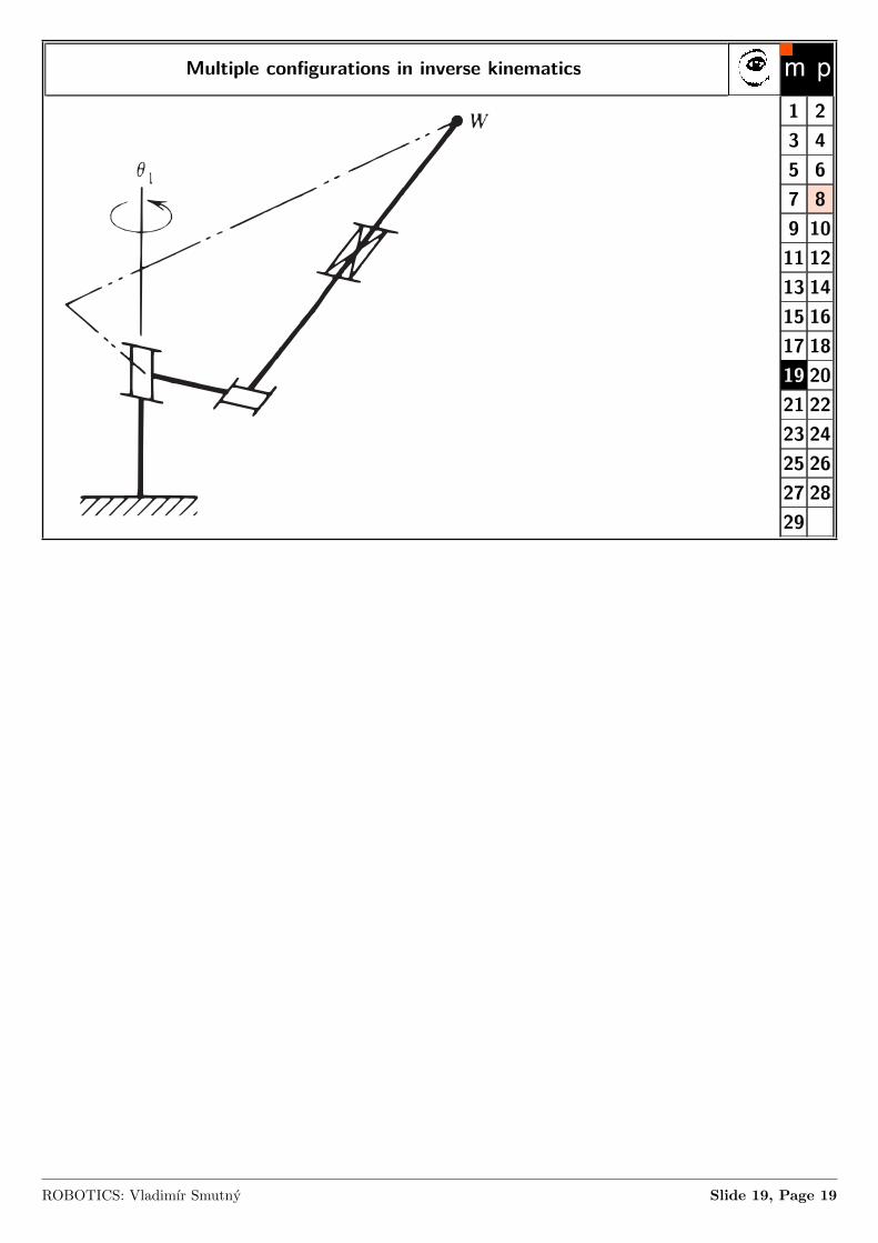
Multiple configurations in inverse kinematics
1 23 45 67 89 1011 1213 1415 1617 1819 2021 2223 2425 2627 2829
ROBOTICS: Vladimır Smutny Slide 19, Page 19
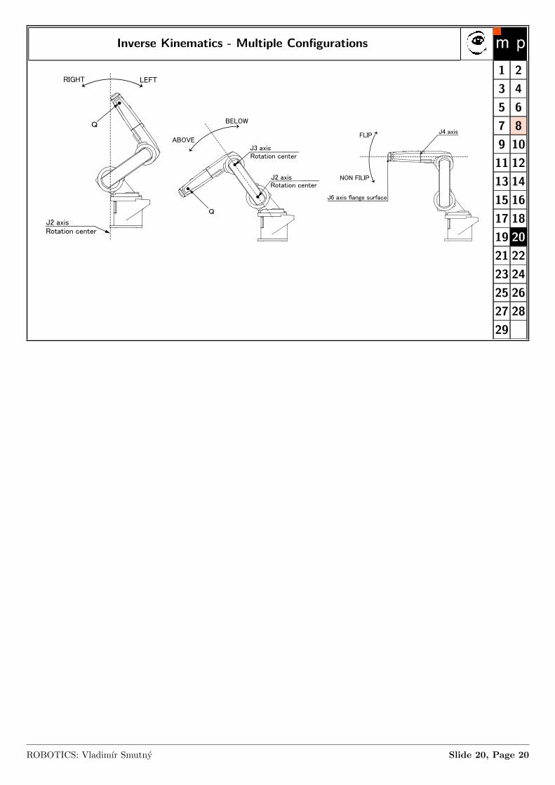
Inverse Kinematics - Multiple Configurations
6Appendix
Configuration flag Appendix-63
6 Appendix
Appendix 1 : Configuration flag
The configuration flag indicates the robot posture.
For the 6-axis type robot, the robot hand end is saved with the position data configured of X, Y, Z, A, B and C. However, even with the same position data, there are several postures that the robot can change to. The posture is expressed by this configuration flag, and the posture is saved with FL1 in the position constant (X, Y, Z, A, B, C) (FL1, FL2).
The types of configuration flags are shown below.
(1) RIGHT/LEFTQ is center of J5 axis rotation in comparison with the plane through the J2 axis vertical to the ground. .
Fig.6-1 : Configuration flag (RIGHT/LEFT)
(2) ABOVE/BELOWQ is center of J5 axis rotation in comparison with the plane through both the J3 and the J2 axis. .
Fig.6-2 : Configuration flag (ABOVE/BELOW)
RIGHT LEFT
Q
J2 axisRotation center
F L 1 (Flag 1 )
& B 0 0 0 0 0 0 0 0
↑
1 / 0 = R I G H T / L E F T
Note) "&B" is shows the binary
J2 axisRotation center
J3 axisRotation center
Q
ABOVE
BELOW F L 1 (Flag 1 )
& B 0 0 0 0 0 0 0 0
↑
1 / 0 = A B O V E / B E L OW
Note) "&B" is shows the binary
Appendix-64 Configuration flag
6Appendix
(3) NONFLIP/FLIP (6-axis robot only.)This means in which side the J6 axis is in comparison with the plane through both the J4 and the J5 axis..
Fig.6-3 : Configuration flag (NONFLIP/FLIP)
J4 axis
J6 axis flange surface
FLIP
NON FILIP
F L 1 (Flag 1 )
& B 0 0 0 0 0 0 0 0
↑
1 / 0 = N O N F L I P / F L I P
Note) "&B" is shows the binary
1 23 45 67 89 1011 1213 1415 1617 1819 2021 2223 2425 2627 2829
ROBOTICS: Vladimır Smutny Slide 20, Page 20
Example: Multiple configurations for simple planar manipulator
l2
x
φ
y
l1
2 solutions
��
��������
��
��������
����
solutions = singular point8
= singular surface1 (double) solution
����
2 solutions
����
Working envelope
0 solutions
solutions = singular point8
= singular surface1 (double) solution
−1 −0.8 −0.6 −0.4 −0.2 0 0.2 0.4 0.6 0.8 1−1−0.5
00.5
1−200
0
200
400
600
800
1000
y
Working space of the 2DOF planar RR manipulator l1=0.5,l2=0.5
x
φ [d
egre
es]
1 23 45 67 89 1011 1213 1415 1617 1819 2021 2223 2425 2627 2829
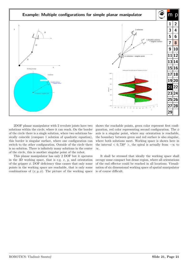
2DOF planar manipulator with 2 revolute joints have twosolutions within the circle, where it can reach. On the borderof the circle there is a single solution, where two solutions ba-sically coincide (compare 1 solution of quadratic equation),this border is singular surface, where one configuration canswitch to the other configuration. Outside of the circle thereis no solution. There is infinitely many solutions in the centerof the circle, this is another singular point of the robot.
This planar manipulator has only 2 DOF but it operatesin the 3D working space, that is e.g. x, y, and orientationof the gripper φ. DOF deficiency thus causes that only somepoints in the working space are reachable, that is only somecombinations of (x, y, φ). The picture of the working space
shows the reachable points, green color represent first confi-guration, red color representing second configuration. The φaxis is a singular point, where any orientation is reachable,the boundary between green and red surface is also singular,where both solutions meet. Working space is shown here inthe interval < 0, 720o >, the spiral is actually from −∞ to∞.
It shall be stressed that ideally the working space shalloccupy some compact but dense region, where all orientationsof the end effector could be reached in all locations. Visuali-sation of six dimensional working space of spatial manipulatoris of course difficult.
ROBOTICS: Vladimır Smutny Slide 21, Page 21
Example: Multiple configurations for simple planar manipulator
−1 −0.8 −0.6 −0.4 −0.2 0 0.2 0.4 0.6 0.8 1−1−0.5
00.5
1−200
0
200
400
600
800
1000
y
Working space of the 2DOF planar RR manipulator l1=0.3,l2=0.7
x
φ [d
egre
es]
−1 −0.8 −0.6 −0.4 −0.2 0 0.2 0.4 0.6 0.8 1−1−0.5
00.5
1−200
0
200
400
600
800
1000
y
Working space of the 2DOF planar RR manipulator l1=0.7,l2=0.3
x
φ [d
egre
es]
l1
l2
φ
x
y
l1
φ
l2
x
y
1 23 45 67 89 1011 1213 1415 1617 1819 2021 2223 2425 2627 2829
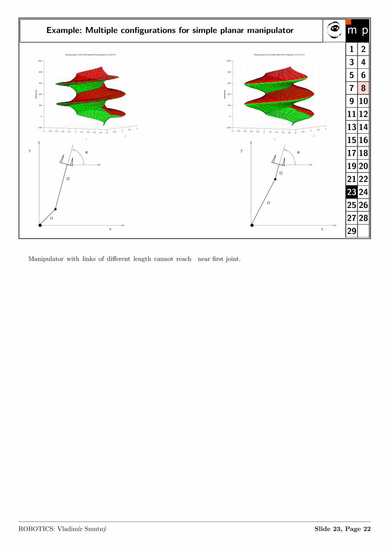
Manipulator with links of different length cannot reach near first joint.
ROBOTICS: Vladimır Smutny Slide 23, Page 22
PUMA
1 23 45 67 89 1011 1213 1415 1617 1819 2021 2223 2425 2627 2829
ROBOTICS: Vladimır Smutny Slide 26, Page 23
Mapping between Joint and Working space
Joints space ⇔ Working (Cartezian) space
0 1 2 3 4 5 6 70
1
2
3
4
5
6
7joint space
θ1
θ 2
⇒ −6 −4 −2 0 2 4 6−6
−4
−2
0
2
4
6working space
x
y
−3 −2 −1 0 1 2 3
−1
−0.5
0
0.5
1
1.5
2
2.5
3
3.5
4
joint space
θ1
θ 2
⇐ −6 −4 −2 0 2 4 6−6
−4
−2
0
2
4
6working space
x
y
1 23 45 67 89 1011 1213 1415 1617 1819 2021 2223 2425 2627 2829
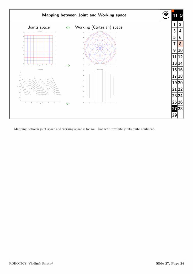
Mapping between joint space and working space is for ro- bot with revolute joints quite nonlinear.
ROBOTICS: Vladimır Smutny Slide 27, Page 24
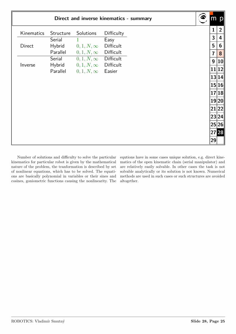
Direct and inverse kinematics - summary
Kinematics Structure Solutions DifficultySerial 1 Easy
Direct Hybrid 0, 1, N,∞ DifficultParallel 0, 1, N,∞ DifficultSerial 0, 1, N,∞ Difficult
Inverse Hybrid 0, 1, N,∞ DifficultParallel 0, 1, N,∞ Easier
1 23 45 67 89 1011 1213 1415 1617 1819 2021 2223 2425 2627 2829
Number of solutions and difficulty to solve the particularkinematics for particular robot is given by the mathematicalnature of the problem, the tranformation is described by setof nonlinear equations, which has to be solved. The equati-ons are basically polynomial in variables or their sines andcosines, goniometric functions causing the nonlinearity. The
equtions have in some cases unique solution, e.g. direct kine-matics of the open kinematic chain (serial manipulator) andare relatively easily solvable. In other cases the task is notsolvable analytically or its solution is not known. Numericalmethods are used in such cases or such structures are avoidedaltogether.
ROBOTICS: Vladimır Smutny Slide 28, Page 25
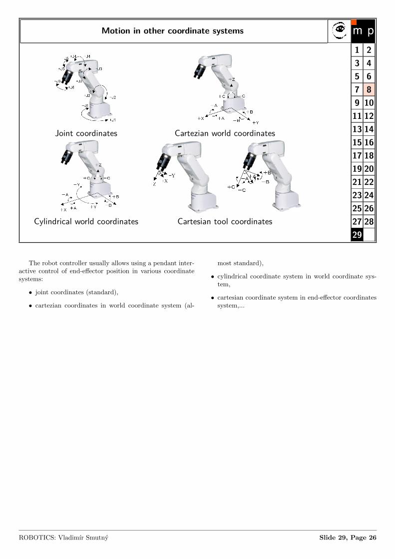
Motion in other coordinate systems
Joint coordinates Cartezian world coordinates
Cylindrical world coordinates Cartesian tool coordinates
1 23 45 67 89 1011 1213 1415 1617 1819 2021 2223 2425 2627 2829
The robot controller usually allows using a pendant inter-active control of end-effector position in various coordinatesystems:
• joint coordinates (standard),
• cartezian coordinates in world coordinate system (al-
most standard),
• cylindrical coordinate system in world coordinate sys-tem,
• cartesian coordinate system in end-effector coordinatessystem,...
ROBOTICS: Vladimır Smutny Slide 29, Page 26


![Inverse Kinematics and Gaze Stabilization for the Rochester ......3 Inverse Kinematics 3.1 Inverse Kinematics: O,A,T from TOOL The mathematics in [Brown and Rimey, 1988] Section 9](https://img.pdfslide.net/doc/110x75/60be15e583990e1ab8600327/inverse-kinematics-and-gaze-stabilization-for-the-rochester-3-inverse-kinematics.jpg)