Kinematics analysis of the parallel module of the

VERNE machine

Daniel Kanaan, Philippe Wenger, Damien Chablat

To cite this version:

Daniel Kanaan, Philippe Wenger, Damien Chablat. Kinematics analysis of the parallel mod-ule of the VERNE machine. Jun 2007, Besancon, France. IFTOMM, pp.1-6, 2007. <hal-00145391>

HAL Id: hal-00145391

https://hal.archives-ouvertes.fr/hal-00145391

Submitted on 10 May 2007

HAL is a multi-disciplinary open accessarchive for the deposit and dissemination of sci-entific research documents, whether they are pub-lished or not. The documents may come fromteaching and research institutions in France orabroad, or from public or private research centers.

L’archive ouverte pluridisciplinaire HAL, estdestinee au depot et a la diffusion de documentsscientifiques de niveau recherche, publies ou non,emanant des etablissements d’enseignement et derecherche francais ou etrangers, des laboratoirespublics ou prives.

12th IFToMM World Congress, Besançon (France), June18-21, 2007 CK-xxx

1

Kinematics analysis of the parallel module of the VERNE machine

D. Kanaan* Ph. Wenger

† D. Chablat

‡

Institut de Recherche en Communications et Cybernétique de Nantes,

UMR CNRS 6597, 1 rue de la Noë, 44321 Nantes, France

Abstract—The paper derives the inverse and forward

kinematic equations of a spatial three-degree-of-freedom

parallel mechanism, which is the parallel module of a hybrid

serial-parallel 5-axis machine tool. This parallel mechanism

consists of a moving platform that is connected to a fixed base by

three non-identical legs. Each leg is made up of one prismatic

and two pair spherical joint, which are connected in a way that

the combined effects of the three legs lead to an over-

constrained mechanism with complex motion. This motion is

defined as a simultaneous combination of rotation and

translation.

Keywords: Parallel manipulators, Parallel kinematic

machines, inverse kinematics, forward kinematics, complex

motion.

I. Introduction

Parallel kinematic machines (PKM) are known for their

high structural rigidity, better payload-to-weight ratio,

high dynamic performances and high accuracy [1], [2],

[3]. Thus, they are prudently considered as attractive

alternatives designs for demanding tasks such as high-

speed machining [4].

Most of the existing PKM can be classified into two

main families. The PKM of the first family have fixed

foot and variable–length struts, while the PKM of the

second family have fixed length struts with moveable foot

points gliding on fixed linear joints [5].

In the first family, we distinguish between PKM with six

degrees of freedom generally called Hexapods and PKM

with three degrees of freedom called Tripods [6], [7].

Hexapods have a Stewart–Gough parallel kinematic

architecture. Many prototypes and commercial hexapod

PKM already exist, including the VARIAX (Gidding and

Lewis), the TORNADO 2000 (Hexel).

We can also find hybrid architectures like the TRICEPT

machine from Neos-robotics [8] which is composed of a

two-axis wrist mounted in series to a 3-DOF “tripod”

positioning structure.

In the second family, we find the HEXAGLIDE (ETH

Zürich) which features six parallel and coplanar linear

joints. The HexaM (Toyoda) is another example with

three pairs of adjacent linear joints lying on a vertical cone

[9]. A hybrid parallel/kinematic PKM with three inclined

linear joints and a two-axis wrist is the GEORGE V (IFW

* E-mail: daniel.kanaan@irccyn.ec-nantes.fr

† E-mail: philippe.wenger@irccyn.ec-nantes.fr ‡ E-mail: damien.chablat@irccyn.ec-nantes.fr

Uni Hanover).

Many three-axis translational PKMs belong to this second

family and use architecture close to the linear Delta robot

originally designed by Clavel for pick-and-place

operations [10]. The Urane SX (Renault Automation) and

the QUICKSTEP (Krause and Mauser) have three non-

coplanar horizontal linear joints [11].

Many researches have made contributions to the study

of the kinematics of these PKMs. Most of these articles

focused on the discussion of both the analytical and

numerical methods [12], [13].

The purpose of this paper is to formulate analytic

expressions in order to find all possible solutions for the

inverse and forward kinematics problem of the VERNE

machine. Then we identify these solutions in order to find

the solution that satisfies the end-user.

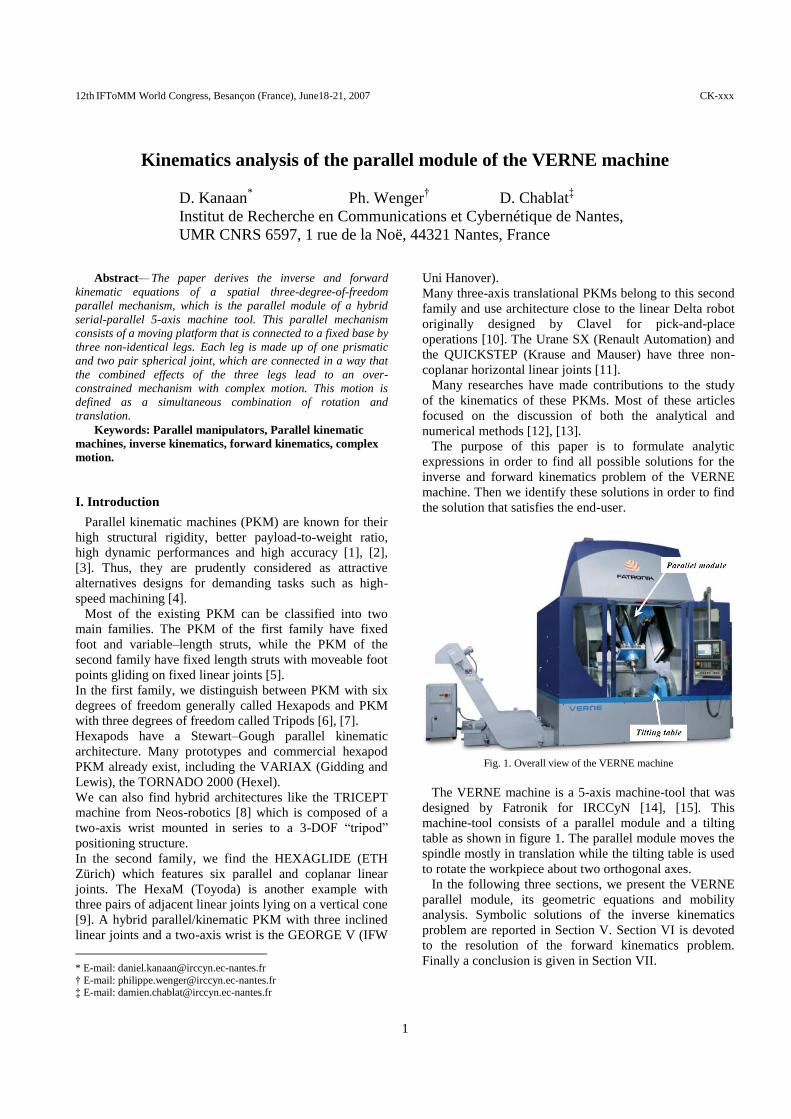
Fig. 1. Overall view of the VERNE machine

The VERNE machine is a 5-axis machine-tool that was

designed by Fatronik for IRCCyN [14], [15]. This

machine-tool consists of a parallel module and a tilting

table as shown in figure 1. The parallel module moves the

spindle mostly in translation while the tilting table is used

to rotate the workpiece about two orthogonal axes.

In the following three sections, we present the VERNE

parallel module, its geometric equations and mobility

analysis. Symbolic solutions of the inverse kinematics

problem are reported in Section V. Section VI is devoted

to the resolution of the forward kinematics problem.

Finally a conclusion is given in Section VII.

12th IFToMM World Congress, Besançon (France), June18-21, 2007 CK-xxx

2

II. Description and mobility of the parallel module

Fig. 2. Schematic representation of the parallel module

Figure 2 shows a scheme of the parallel module of the

VERNE machine. The kinematic architecture can be

described by a simple scheme shown in figure 3, where

joints are represented by rectangles and links between

those joints are represented by lines (P and S indicate

prismatic and spherical joint, respectively). The moving

platform is rectangular. The vertices of this platform are

connected to a fixed-base plate through three legs Ι, ΙΙ and

ΙΙΙ. Each leg uses pairs of rods linking a prismatic joint to

the moving platform through two pair spherical joints.

Legs ΙΙ and ΙΙΙ are two identical parallelograms. Leg Ι

differs from the other two legs in that 11 12 11 12A A B B , that

is, it is not an articulated parallelograms. The movement

of the moving platform is generated by the slide of three

actuators along three vertical guideways.

ss

ss

ss

ss

ss

ss

P

P

P

Bas

e

Pla

tfo

rm

Fig. 3. Joints and loops graph of VERNE

Using the Grubler formula recalled in Equation (1), it

can be proved that the mobility m of the platform is equal

to three:

int

1

6 1tN

p t i

i

m N N f m

(1)

where m denotes the mobility of the manipulator, pN is

the total number of rigid bodies of the manipulator,

11pN for 3 piston-rods, one base, one moving platform

and 6 rods. tN is the number of the joints, 15tN for 12

spherical joints S, 3 prismatic joints P. if denotes the

number of degrees of freedom (DOF) of the thi joint, and

mint is the number of internal DOF, which do not influence

the motion of manipulator.

Based on equation (1), the mobility of the platform is

given by 6 11 15 1 39 6 3m .

Due to the arrangement of the links and joints, as shown

in figure 2, legs ΙΙ and ΙΙΙ prevent the platform from

rotating about y and z axes. Leg Ι prevents the platforms

from rotating about z-axis but, because 11 12 11 12A A B B , a

slight coupled rotation about x-axis exists.

III. Kinematic equations

In order to analyse the kinematics of our parallel

module, two relative coordinates are assigned as shown in

figures 2. A static Cartesian frame xyz is fixed at the base

of the machine tool, with the z-axis pointing downward

along the vertical direction. The mobile Cartesian frame,

P P Px y z , is attached to the moving platform at point P and

remains parallel to xyz.

In any constrained mechanical system, joints connecting

bodies restrict their relative motion and impose constraints

on the generalized coordinates, geometric constraints are

then formulated as algebraic expressions involving

generalized coordinates.

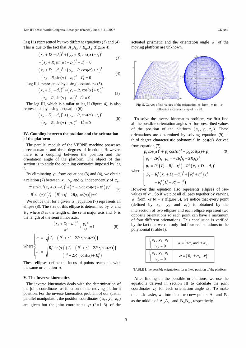
Fig. 4. Dimensions of the parallel kinematic structure in the frame

supplied by Fatronik

Using the parameters defined in figure 4, the constraint

equations of the parallel manipulator are expressed as:

2 2 2

2 0Bij Aij Bij Aij Bij Aij ix x y y z z L (2)

where ijA (respectively ijB ) is the center of spherical joint

number j on the prismatic joint number i (respectively on

the moving platform side), i = 1..3, j = 1..2.

12th IFToMM World Congress, Besançon (France), June18-21, 2007 CK-xxx

3

Leg Ι is represented by two different equations (3) and (4).

This is due to the fact that 11 12 11 12A A B B (figure 4).

2 2

1 1 1 1

2 2

1 1 1

cos( )

sin( ) 0

P P

P

x D d y R r

z R L

(3)

2 2

1 1 1 1

2 2

1 1 1

cos( )

sin( ) 0

P P

P

x D d y R r

z R L

(4)

Leg ΙΙ is represented by a single equations (5).

2 2

2 2 2 4

2 2

2 2 2

cos( )

sin( ) - 0

P P

P

x D d y R r

z R L

(5)

The leg ІІІ, which is similar to leg ІІ (figure 4), is also

represented by a single equation (6).

2 2

2 2 2 4

2 2

2 3 3

cos( )

sin( ) 0

P P

P

x D d y R r

z R L

(6)

IV. Coupling between the position and the orientation

of the platform

The parallel module of the VERNE machine possesses

three actuators and three degrees of freedom. However,

there is a coupling between the position and the

orientation angle of the platform. The object of this

section is to study the coupling constraint imposed by leg

I.

By eliminating 1 from equations (3) and (4), we obtain

a relation (7) between , and P Px y independently of Pz .

22 2 2 2 2

1 1 1 1 1 1 1

2 2 2 2 2

1 1 1 1 1 1

sin( ) 2 cos( )

sin( ) 2 cos( ) 0

P PR x D d r R r R y

R L R r R r

(7)

We notice that for a given , equation (7) represents an

ellipse (8). The size of this ellipse is determined by a and

b , where a is the length of the semi major axis and b is

the length of the semi minor axis.

2 21 1

2 21

P Px D d y

a b

(8)

where

2 2 2

1 1 1 1 1

2 2 2 2 2

1 1 1 1 1 1

2 2

1 1 1 1

2 cos( )

sin( ) 2 cos( )

2 cos( )

a L R r R r

R L R r R rb

r R r R

These ellipses define the locus of points reachable with

the same orientation .

V. The Inverse kinematics

The inverse kinematics deals with the determination of

the joint coordinates as function of the moving platform

position. For the inverse kinematics problem of our spatial

parallel manipulator, the position coordinates ( , , P P Px y z )

are given but the joint coordinates ( 1..3)i i of the

actuated prismatic and the orientation angle of the

moving platform are unknown.

Fig. 5. Curves of iso-values of the orientation from - to

following a constant step of / 90.

To solve the inverse kinematics problem, we first find

all the possible orientation angles for prescribed values

of the position of the platform ( , , P P Px y z ). These

orientations are determined by solving equation (9), a

third degree characteristic polynomial in cos( ) derived

from equation (7).

3 2

1 2 3 4cos( ) cos( ) cos( )p p p p (9)

where

3 3 2

1 1 1 3 1 1 1 1

22 2 2 2 2

2 1 1 1 1 1 1 1

22 2 2 2

4 1 1 1 1 1

2 2 2 2

1 1 1 1

2 , 2 2

P

P

P P

p R r p R r R r y

p R L R r R x D d

p R x D d R r y

R L R r

However this equation also represents ellipses of iso-

values of . So if we plot all ellipses together by varying

from - to (figure 5), we notice that every point

(defined by ,Px Py and

Pz ) is obtained by the

intersection of two ellipses and each ellipse represent two

opposite orientations so each point can have a maximum

of four different orientations. This conclusion is verified

by the fact that we can only find four real solutions to the

polynomial (Table I).

, ,

0

P P P

P

x y z

y

1 2

and

, ,

0

P P P

P

x y z

y

10, ,

TABLE I. the possible orientations for a fixed position of the platform

After finding all the possible orientations, we use the

equations derived in section III to calculate the joint

coordinates i for each orientation angle . To make

this task easier, we introduce two new points 1A and

1B

as the middle of 11 12A A and

11 12B B , respectively.

12th IFToMM World Congress, Besançon (France), June18-21, 2007 CK-xxx

4

2 22

1 1 1

2 2 2

1 1 1 1 12 cos( ) 0

P P Px D d y z

L R r R r

(10)

Then, for prescribed values of the position and orientation

of the platform, the required actuator inputs can be

directly computed from equations (10), (5) and (6):

2 2 2

1 1 1 1 1

1 12 2

1 1

2 cos( )

-P

P P

L R r R rz s

x D d y

(11)

22

2 2 2

2 2 2 2

2 4

sin( )cos( )

P

P

P

L x D dz R s

y R r

(12)

22

3 2 2

3 2 3 2

2 4

sin( )cos( )

P

P

P

L x D dz R s

y R r

(13)

where 1 2 3, , 1s s s are the configuration indices

defined as the signs of 1 Pz ,

2 2 sin( )Pz R ,

3 2 sin( )Pz R , respectively.

Subtracting equation (3) from equation (4), yields:

P 1 1 1 1 P

y R cos( ) r =R sin( ) z (14)

1 1 P1(14) sgn sgn sin( ) sgn R cos( ) r sgn(y )pz

This means that for prescribed values of the position and

orientation of the platform, the joint coordinate 1

possesses one solution, except when {0, }. In this

case 1s can take on both values +1 and –1. As a result

1

can take on two values when {0, }.

0, 1 1s

1 1

p

cos( )

y 0 with 0

R r

1 pz

others 1 1 or -1s

TABLE II. the solution of the joint coordinate 1 according to the

values of

Observing equations (11), (12), (13), Table I and Table

II, we conclude that the three legs, with four postures for

leg Ι and two postures for leg ΙΙ and ΙΙΙ results in sixteen

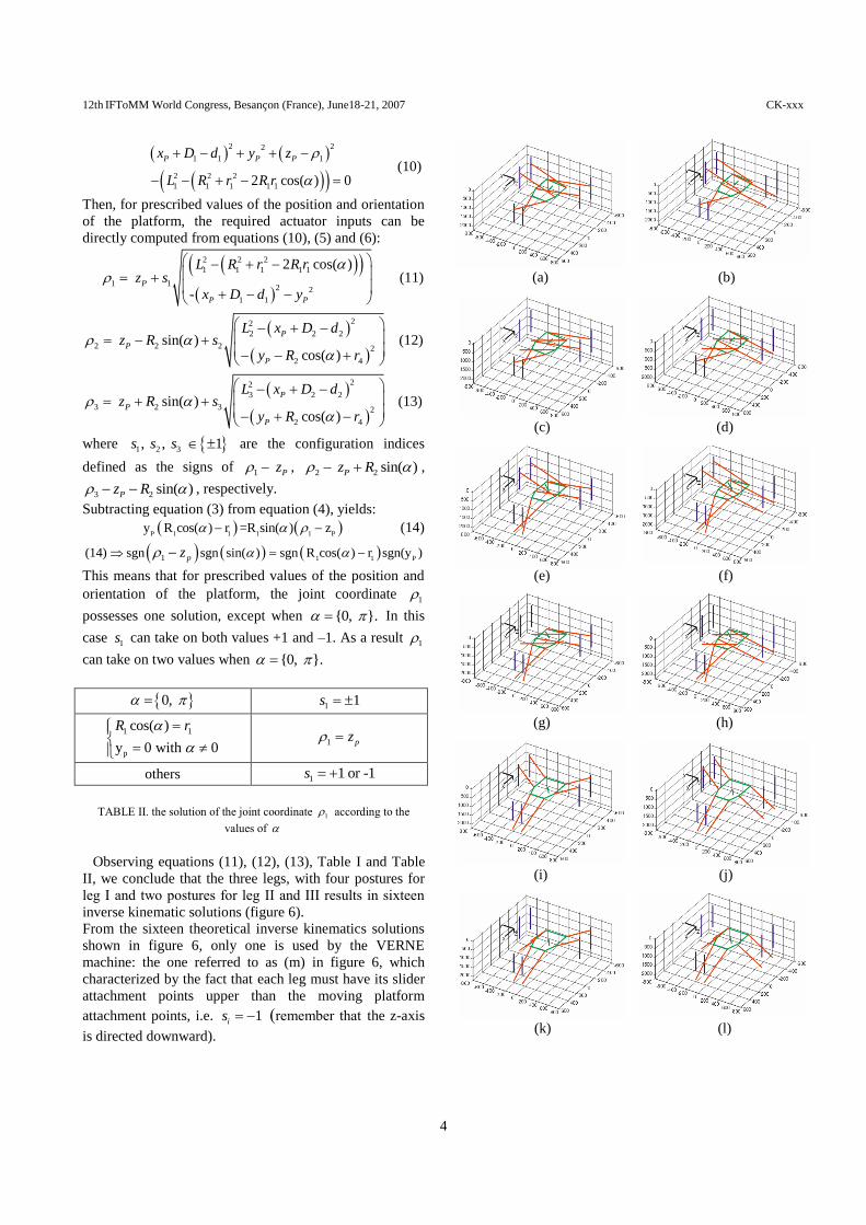
inverse kinematic solutions (figure 6).

From the sixteen theoretical inverse kinematics solutions

shown in figure 6, only one is used by the VERNE

machine: the one referred to as (m) in figure 6, which

characterized by the fact that each leg must have its slider

attachment points upper than the moving platform

attachment points, i.e. 1is (remember that the z-axis

is directed downward).

(a) (b)

(c) (d)

(e) (f)

(g) (h)

(i) (j)

(k) (l)

12th IFToMM World Congress, Besançon (France), June18-21, 2007 CK-xxx

5

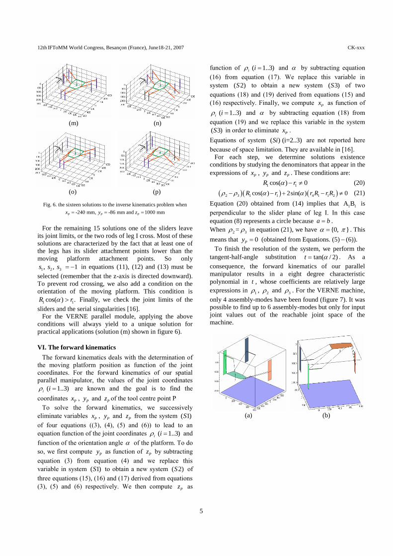
(m) (n)

(o) (p)

Fig. 6. the sixteen solutions to the inverse kinematics problem when

-240 mm, -86 mm and 1000 mmP P Px y z

For the remaining 15 solutions one of the sliders leave

its joint limits, or the two rods of leg I cross. Most of these

solutions are characterized by the fact that at least one of

the legs has its slider attachment points lower than the

moving platform attachment points. So only

1 2 3, , 1s s s in equations (11), (12) and (13) must be

selected (remember that the z-axis is directed downward).

To prevent rod crossing, we also add a condition on the

orientation of the moving platform. This condition is

1 1cos( ) .R r Finally, we check the joint limits of the

sliders and the serial singularities [16].

For the VERNE parallel module, applying the above

conditions will always yield to a unique solution for

practical applications (solution (m) shown in figure 6).

VI. The forward kinematics

The forward kinematics deals with the determination of

the moving platform position as function of the joint

coordinates. For the forward kinematics of our spatial

parallel manipulator, the values of the joint coordinates

( 1..3)i i are known and the goal is to find the

coordinates Px ,

Py and Pz of the tool centre point P

To solve the forward kinematics, we successively

eliminate variables Px ,

Py and Pz from the system ( 1)S

of four equations ((3), (4), (5) and (6)) to lead to an

equation function of the joint coordinates ( 1..3)i i and

function of the orientation angle of the platform. To do

so, we first compute Py as function of

Pz by subtracting

equation (3) from equation (4) and we replace this

variable in system ( 1)S to obtain a new system ( 2)S of

three equations (15), (16) and (17) derived from equations

(3), (5) and (6) respectively. We then compute Pz as

function of ( 1..3)i i and by subtracting equation

(16) from equation (17). We replace this variable in

system ( 2)S to obtain a new system ( 3)S of two

equations (18) and (19) derived from equations (15) and

(16) respectively. Finally, we compute Px as function of

( 1..3)i i and by subtracting equation (18) from

equation (19) and we replace this variable in the system

( 3)S in order to eliminate Px .

Equations of system ( ) (i=2..3)Si are not reported here

because of space limitation. They are available in [16].

For each step, we determine solutions existence

conditions by studying the denominators that appear in the

expressions of Px ,

Py and Pz . These conditions are:

1 1cos( ) 0R r (20)

2 3 1 1 4 1 1 2cos( ) 2sin( ) 0R r r R r R (21)

Equation (20) obtained from (14) implies that 1 1A B is

perpendicular to the slider plane of leg І. In this case

equation (8) represents a circle because a b .

When 2 3= in equation (21), we have {0, } . This

means that 0Py (obtained from Equations. (5) (6)).

To finish the resolution of the system, we perform the

tangent-half-angle substitution tan( / 2)t . As a

consequence, the forward kinematics of our parallel

manipulator results in a eight degree characteristic

polynomial in t , whose coefficients are relatively large

expressions in 1 ,

2 and 3 . For the VERNE machine,

only 4 assembly-modes have been found (figure 7). It was

possible to find up to 6 assembly-modes but only for input

joint values out of the reachable joint space of the

machine.

(a) (b)

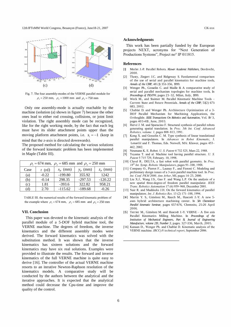
12th IFToMM World Congress, Besançon (France), June18-21, 2007 CK-xxx

6

(c) (d)

Fig. 7. The four assembly-modes of the VERNE parallel module for

1 250 mm, 2 1000 mm and 3 750 mm

Only one assembly-mode is actually reachable by the

machine (solution (a) shown in figure 7) because the other

ones lead to either rod crossing, collisions, or joint limit

violation. The right assembly mode can be recognized,

like for the right working mode, by the fact that each leg

must have its slider attachment points upper than the

moving platform attachment points, i.e. 1is (keep in

mind that the z-axis is directed downwards).

The proposed method for calculating the various solutions

of the forward kinematic problem has been implemented

in Maple (Table III).

1 674 mm, 2 685 mm and

3 250 mm

Case t (rd) Px (mm) Py (mm)

Pz (mm)

(a) -0.22 -199.80 355.92 1242

(b) -0.14 298.35 -297.53 -120.22

(c) 1.81 -393.6 322.82 958.21

(d) 2.70 -115.62 -189.68 -0.26

TABLE III. the numerical results of the forward kinematic problem of

the example where 1 674 mm, 2 685 mm and 3 250 mm

VII. Conclusion

This paper was devoted to the kinematic analysis of the

parallel module of a 5-DOF hybrid machine tool, the

VERNE machine. The degrees of freedom, the inverse

kinematics and the different assembly modes were

derived. The forward kinematics was solved with the

substitution method. It was shown that the inverse

kinematics has sixteen solutions and the forward

kinematics may have six real solutions. Examples were

provided to illustrate the results. The forward and inverse

kinematics of the full VERNE machine is quite easy to

derive [16]. The controller of the actual VERNE machine

resorts to an iterative Newton-Raphson resolution of the

kinematics models. A comparative study will be

conducted by the authors between the analytical and the

iterative approaches. It is expected that the analytical

method could decrease the Cpu-time and improve the

quality of the control.

Acknowledgments

This work has been partially funded by the European

projects NEXT, acronyms for “Next Generation of

Productions Systems”, Project no° IP 011815.

References

[1] Merlet J.-P. Parallel Robots. Kluwer Academic Publishers, Dordrecht,

2000.

[2] Tlusty, Ziegert J.C. and Ridgeway S. Fundamental comparison

of the use of serial and parallel kinematics for machine tools,

Annals of the CIRP, 48 (1) 351–356, 1999.

[3] Wenger Ph., Gosselin C. and Maille B. A comparative study of

serial and parallel mechanism topologies for machine tools, In

Proceedings of PKM’99, pages 23–32, Milan, Italy, 1999.

[4] Weck M., and Staimer M. Parallel Kinematic Machine Tools –

Current State and Future Potentials. Annals of the CIRP, 51(2) 671-

683, 2002.

[5] Chablat D. and Wenger Ph. Architecture O ptimization of a 3-

DO F Parallel Mechanism for Machining Applications, the

O rthoglide. IEEE Transactions On Robotics and Automation, Vol. 19/ 3,

pages 403-410, June, 2003.

[6] Hervé J. M. and Sparacino F. Structural synthesis of parallel robots

generating spatial translation. In Proc. 5th Int. Conf. Advanced Robotics, volume. 1, pages 808–813, 1991.

[7] Kong X. and Gosselin C. M. Type synthesis of linear translational

parallel manipulators. In Advances in Robot Kinematic, J.

Lenarcic

and F. Thomas, Eds. Norwell, MA: Kluwer, pages 453–

462, 2002.

[8] Neumann K. E. Robot. U. S. Patent 4 732 525, Mars 22, 1988. [9] Toyama T. and al. Machine tool having parallel structure. U. S.

Patent 5 715 729, February. 10, 1998.

[10] Clavel R.. DELTA, a fast robot with parallel geometry. In Proc. 18th Int. Symp. Robotic Manipulators, pages 91–100, 1988.

[11] Company O., Pierrot F.., Launay F., and Fioroni C. Modeling and

preliminary design issues of a 3-axis parallel machine tool. In Proc. Int. Conf. PKM 2000, Ann Arbor, MI, pages 14–23, 2000.

[12] Liu X.J., Wang J.S., Gao F. and Wang L.P. On the analysis of a

new spatial three-degree-of freedom parallel manipulator. IEEE Trans. Robotics Automation 17 (6) 959–968, December 2001.

[13] Nair R. and Maddocks J.H. On the forward kinematics of parallel

manipulators. Int. J. Robotics Res. 13 (2) 171–188, 1994.

[14] Martin Y. S., Giménez M., Rauch M., Hascoët J.-Y. A new 5-

axes hybrid architecture machining center. In 5th Chemnitzer

Parallel kinematic Seminar, pages 657-676, Chemnitz, 25-26 April

2006.

[15] Terrier M., Giménez M. and Hascoёt J.-Y. VERNE – A five axis

Parallel Kinematics Milling Machine. In Proceedings of the

Institution of Mechanical Engineers, Part B, Journal of Engineering

Manufacture, volume 219, Number 3, pages. 327-336, March, 2005.

[16] Kanaan D., Wenger Ph. and Chablat D. Kinematic analysis of the

VERNE machine. IRCCyN technical report, September 2006.