P

JJa

b

c

d

e

f

g

a

ARR1AA

KSRGTEM

1

icsomrlsmb

up

0d

Ecological Modelling 221 (2010) 467–478

Contents lists available at ScienceDirect

Ecological Modelling

journa l homepage: www.e lsev ier .com/ locate /eco lmodel

redicting the distributions of marine organisms at the global scale

onathan Readya,∗, Kristin Kaschnerb, Andy B. Southc, Paul D. Eastwoodc, Tony Reesd,osephine Riuse, Eli Agbayanie, Sven Kullander f, Rainer Froeseg

Instituto de Estudos Costeiros, Universidade Federal do Pará – Campus de Braganca, Aldeia, Braganca 68600-000, Pará, BrazilEvolutionary Biology & Ecology Lab, Institute of Biology I (Zoology), Albert-Ludwigs-University Freiburg, GermanyCentre for Environment, Fisheries, and Aquaculture Science (Cefas), Lowestoft Laboratory, Lowestoft, Suffolk, NR33 0HT, UKCSIRO Marine and Atmospheric Research, GPO Box 1538 Hobart TAS 7001, AustraliaWorldFish Center – Philippines Office, MCPO Box 2631, 0718 Makati City, PhilippinesDepartment of Vertebrate Zoology, Swedish Museum of Natural History, Box 50007, 104 05 Stockholm, SwedenLeibniz-Institute of Marine Sciences, Düsternbrooker Weg 20, D-24105 Kiel, Germany

r t i c l e i n f o

rticle history:eceived 20 March 2008eceived in revised form5 September 2009ccepted 16 October 2009vailable online 24 November 2009

eywords:

a b s t r a c t

We present and evaluate AquaMaps, a presence-only species distribution modelling system that allowsthe incorporation of expert knowledge about habitat usage and was designed for maximum output ofstandardized species range maps at the global scale. In the marine environment there is a significant chal-lenge to the production of range maps due to large biases in the amount and location of occurrence datafor most species. AquaMaps is compared with traditional presence-only species distribution modellingmethods to determine the quality of outputs under equivalently automated conditions. The effect of theinclusion of expert knowledge to AquaMaps is also investigated. Model outputs were tested internally,

pecies distribution modellingange mapslobal marine biodiversityrawl surveysxpert reviewodel comparison

through data partitioning, and externally against independent survey data to determine the ability ofmodels to predict presence versus absence. Models were also tested externally by assessing correlationwith independent survey estimates of relative species abundance. AquaMaps outputs compare well tothe existing methods tested, and inclusion of expert knowledge results in a general improvement inmodel outputs. The transparency, speed and adaptability of the AquaMaps system, as well as the exist-ing online framework which allows expert review to compensate for sampling biases and thus improvemodel predictions are proposed as additional benefits for public and research use alike.

. Introduction

Concerns over changing patterns of marine biodiversity result-ng from climate change and human impacts have generatedonsiderable interest in the use of models designed to generatepatial predictions (i.e. maps) of species’ distributions from pointccurrence data (Guisan and Thuiller, 2005). Ideally, predictionodels would be generated from comprehensive species occur-

ence and absence data from targeted surveys. Unfortunately thisevel of data is only available for a relatively limited number ofpecies and geographic locations, creating problems for assess-ents of changes in patterns of marine species distributions and

iodiversity at regional and global scales.As an alternative, modellers are making use of increasing vol-

mes of presence-only data (Pearce and Boyce, 2006). These areublished online through global databases such as FishBase (Froese

∗ Corresponding author. Tel.: +55 0 91 3425 1745; fax: +55 0 91 3425 1209.E-mail address: jonathan.ready@gmail.com (J. Ready).

304-3800/$ – see front matter © 2009 Elsevier B.V. All rights reserved.oi:10.1016/j.ecolmodel.2009.10.025

© 2009 Elsevier B.V. All rights reserved.

and Pauly, 2007) and the Ocean Biogeographic Information Sys-tem (OBIS, 2007), both of which feed data directly into the GlobalBiodiversity Information Facility (GBIF, 2007). These data frame-works compile species occurrence data from museum recordsand other sources. They therefore represent a highly patchy andbiased view of patterns of species’ distributions as a result ofregional and local variations in sampling effort. The bias inherentto the data creates problems when data-driven modelling tech-niques are used to generate predictions of species’ distributions.This is because an absence of occurrence records may not nec-essarily indicate a true absence in the distribution of the species,but rather a lack of adequate sampling. This is especially true formarine organisms, as inshore areas are more often sampled ata higher rate compared to offshore areas, causing a bias in thespecies–habitat relationship described by the data (Kaschner et al.,

2006; MacLeod et al., 2008). In this scenario, an offshore speciesmight well be predicted to have an inshore distribution if sam-pling had only occurred over a limited proportion of its overalldepth range. Similarly, misidentification of species is a commonweakness of all existing large online occurrence record deposi-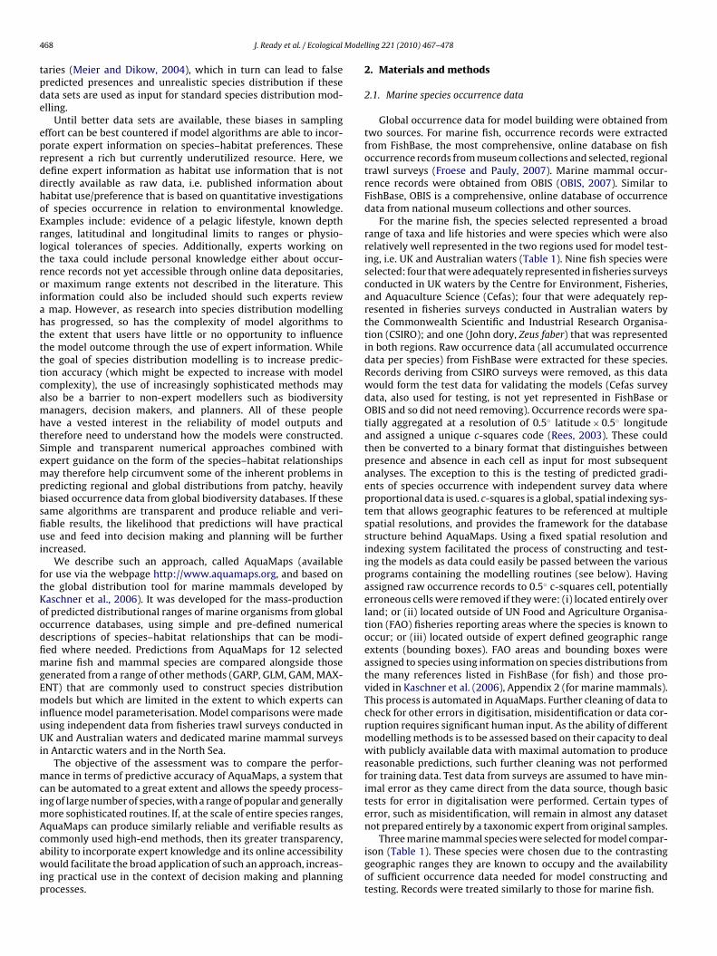

4 Model

tpde

eprddhoErltroiahttttcamhtSempbsfiui

ftKoodfimgEmiuUi

mcimAcawip

68 J. Ready et al. / Ecological

aries (Meier and Dikow, 2004), which in turn can lead to falseredicted presences and unrealistic species distribution if theseata sets are used as input for standard species distribution mod-lling.

Until better data sets are available, these biases in samplingffort can be best countered if model algorithms are able to incor-orate expert information on species–habitat preferences. Theseepresent a rich but currently underutilized resource. Here, weefine expert information as habitat use information that is notirectly available as raw data, i.e. published information aboutabitat use/preference that is based on quantitative investigationsf species occurrence in relation to environmental knowledge.xamples include: evidence of a pelagic lifestyle, known depthanges, latitudinal and longitudinal limits to ranges or physio-ogical tolerances of species. Additionally, experts working onhe taxa could include personal knowledge either about occur-ence records not yet accessible through online data depositaries,r maximum range extents not described in the literature. Thisnformation could also be included should such experts review

map. However, as research into species distribution modellingas progressed, so has the complexity of model algorithms tohe extent that users have little or no opportunity to influencehe model outcome through the use of expert information. Whilehe goal of species distribution modelling is to increase predic-ion accuracy (which might be expected to increase with modelomplexity), the use of increasingly sophisticated methods maylso be a barrier to non-expert modellers such as biodiversityanagers, decision makers, and planners. All of these people

ave a vested interest in the reliability of model outputs andherefore need to understand how the models were constructed.imple and transparent numerical approaches combined withxpert guidance on the form of the species–habitat relationshipsay therefore help circumvent some of the inherent problems in

redicting regional and global distributions from patchy, heavilyiased occurrence data from global biodiversity databases. If theseame algorithms are transparent and produce reliable and veri-able results, the likelihood that predictions will have practicalse and feed into decision making and planning will be further

ncreased.We describe such an approach, called AquaMaps (available

or use via the webpage http://www.aquamaps.org, and based onhe global distribution tool for marine mammals developed byaschner et al., 2006). It was developed for the mass-productionf predicted distributional ranges of marine organisms from globalccurrence databases, using simple and pre-defined numericalescriptions of species–habitat relationships that can be modi-ed where needed. Predictions from AquaMaps for 12 selectedarine fish and mammal species are compared alongside those

enerated from a range of other methods (GARP, GLM, GAM, MAX-NT) that are commonly used to construct species distributionodels but which are limited in the extent to which experts can

nfluence model parameterisation. Model comparisons were madesing independent data from fisheries trawl surveys conducted inK and Australian waters and dedicated marine mammal surveys

n Antarctic waters and in the North Sea.The objective of the assessment was to compare the perfor-

ance in terms of predictive accuracy of AquaMaps, a system thatan be automated to a great extent and allows the speedy process-ng of large number of species, with a range of popular and generally

ore sophisticated routines. If, at the scale of entire species ranges,quaMaps can produce similarly reliable and verifiable results as

ommonly used high-end methods, then its greater transparency,bility to incorporate expert knowledge and its online accessibilityould facilitate the broad application of such an approach, increas-

ng practical use in the context of decision making and planningrocesses.

ling 221 (2010) 467–478

2. Materials and methods

2.1. Marine species occurrence data

Global occurrence data for model building were obtained fromtwo sources. For marine fish, occurrence records were extractedfrom FishBase, the most comprehensive, online database on fishoccurrence records from museum collections and selected, regionaltrawl surveys (Froese and Pauly, 2007). Marine mammal occur-rence records were obtained from OBIS (OBIS, 2007). Similar toFishBase, OBIS is a comprehensive, online database of occurrencedata from national museum collections and other sources.

For the marine fish, the species selected represented a broadrange of taxa and life histories and were species which were alsorelatively well represented in the two regions used for model test-ing, i.e. UK and Australian waters (Table 1). Nine fish species wereselected: four that were adequately represented in fisheries surveysconducted in UK waters by the Centre for Environment, Fisheries,and Aquaculture Science (Cefas); four that were adequately rep-resented in fisheries surveys conducted in Australian waters bythe Commonwealth Scientific and Industrial Research Organisa-tion (CSIRO); and one (John dory, Zeus faber) that was representedin both regions. Raw occurrence data (all accumulated occurrencedata per species) from FishBase were extracted for these species.Records deriving from CSIRO surveys were removed, as this datawould form the test data for validating the models (Cefas surveydata, also used for testing, is not yet represented in FishBase orOBIS and so did not need removing). Occurrence records were spa-tially aggregated at a resolution of 0.5◦ latitude × 0.5◦ longitudeand assigned a unique c-squares code (Rees, 2003). These couldthen be converted to a binary format that distinguishes betweenpresence and absence in each cell as input for most subsequentanalyses. The exception to this is the testing of predicted gradi-ents of species occurrence with independent survey data whereproportional data is used. c-squares is a global, spatial indexing sys-tem that allows geographic features to be referenced at multiplespatial resolutions, and provides the framework for the databasestructure behind AquaMaps. Using a fixed spatial resolution andindexing system facilitated the process of constructing and test-ing the models as data could easily be passed between the variousprograms containing the modelling routines (see below). Havingassigned raw occurrence records to 0.5◦ c-squares cell, potentiallyerroneous cells were removed if they were: (i) located entirely overland; or (ii) located outside of UN Food and Agriculture Organisa-tion (FAO) fisheries reporting areas where the species is known tooccur; or (iii) located outside of expert defined geographic rangeextents (bounding boxes). FAO areas and bounding boxes wereassigned to species using information on species distributions fromthe many references listed in FishBase (for fish) and those pro-vided in Kaschner et al. (2006), Appendix 2 (for marine mammals).This process is automated in AquaMaps. Further cleaning of data tocheck for other errors in digitisation, misidentification or data cor-ruption requires significant human input. As the ability of differentmodelling methods is to be assessed based on their capacity to dealwith publicly available data with maximal automation to producereasonable predictions, such further cleaning was not performedfor training data. Test data from surveys are assumed to have min-imal error as they came direct from the data source, though basictests for error in digitalisation were performed. Certain types oferror, such as misidentification, will remain in almost any datasetnot prepared entirely by a taxonomic expert from original samples.

Three marine mammal species were selected for model compar-ison (Table 1). These species were chosen due to the contrastinggeographic ranges they are known to occupy and the availabilityof sufficient occurrence data needed for model constructing andtesting. Records were treated similarly to those for marine fish.

J. Ready et al. / Ecological Modelling 221 (2010) 467–478 469

Table 1Marine fish and mammal species occurrence data used for model training and survey data used for model testing. Common name taken from FishBase (for fishes) and OBIS(for mammals).

Species code Species name Common name Category Characteristicdescription

Model training data(# presence cells)

Test data region Model testing data

Presences(# cells)

Absences(# cells)

Prevalence

HYPLA Hyperoodon planifrons Southernbottlenose whale

Mammal Beaked whale 37 Southern Oceans 468 12,425 0.04

CAEQU Carangoides equula Whitefin trevally Fish Benthopelagic 40 Australia 49 246 0.17PSERU Psettodes erumei Indian spiny

turbotFish Flatfish 100 Australia 87 248 0.26

CLHAR Clupea harengus Herring Fish Small pelagic 119 UK 213 353 0.38SASAG Sardinops sagax South American

pilchardFish Small pelagic 128 Australia 32 80 0.29

SOSOL Solea solea Common sole Fish Flatfish 140 UK 104 115 0.47TRTRA Trachurus trachurus Horse mackerel Fish Benthopelagic 157 UK 294 353 0.45SQMEG Squalus megalops Shortnose spurdog Fish Elasmobranch 216 Australia 70 260 0.21

lagic

anchale

2

paapaRtba

•

•

•

•

•

hcunmta

ZEFAB Zeus faber John dory Fish BenthopePHPHO Phocoena phocoena Harbour porpoise Mammal PorpoiseSQACA Squalus acanthias Piked dogfish Fish ElasmobrBAPHY Balaenoptera physalus Fin whale Mammal Baleen wh

.2. Environmental data

The following global coverage environmental datasets wererepared at 0.5◦ resolution (259,200 cells). The intention was togglomerate global maps of a number of key environmental vari-bles based on long-term average conditions using comprehensive,ublicly accessible raster data. All geospatial data manipulation andnalysis was performed using ArcMap v.9 (Environmental Systemsesearch Institute). Data is generally available at greater resolu-ions than the 0.5◦ resolution used here, and was converted to suchy calculating mean, minimum and maximum values, and used asppropriate for mean, minimum and maximum layers.

Maximum, minimum, and mean depths. Data were extractedfrom the global coverage ETOPO2 2 min resolution bathymetrydataset (NOAA, 2006).Mean annual sea surface temperature (SST) in degrees Celsiuscovering the period 1982–1999. Data were extracted from a cli-matology produced following the methods described by Reynoldsand Smith (1995) and published by NOAA (2007).Mean annual salinity covering the period 1982–1999. Data wereextracted from the 2001 World Ocean Atlas (Conkright et al.,2002) published by NOAA.Mean annual proportional ice cover (by area) on a scaleof 0.00–1.00 and covering the period 1990–1999. Data wereobtained from the U.S. National Snow and Ice Data Centre(Cavalieri et al., 2006). Inverse distance weighted interpolationwas performed to fill missing data values in a small number ofcoastal cells (approximately 1000 cells).Mean annual primary production in mg C m−2 day−1 for theperiod 1997–2004. Data were obtained from the European JointResearch Council (http://marine.jrc.ec.europa.eu/made availableby Frédéric Mélin) having been generated from remotely sensedchlorophyll a concentrations using an approach described in Carret al. (2006).

The environmental datasets and metadata are freely available atttp://www.aquamaps.org. Data sets were chosen for their appli-ability at the global scale and likely variability at the resolution

sed. Slope and terrain variability measures were considered, butot used. This is because their value for modelling pelagic speciesay not be good, their variability within cells at the 0.5◦ resolu-

ion may be very great, and there was a desire to maintain claritynd transparency by using only a moderate number of layers. Max-

502 Australia and UK 153 565 0.21509 North East Atlantic 177 457 0.281468 UK 219 353 0.381949 Southern Oceans 102 12,425 0.01

imum and minimum values for SST, salinity, proportional ice coverand primary production are also available but represent temporalvariation within the cell rather than physical variation (as in thecase of depth). For simplicity and transparency they have not beenincluded.

2.3. Test data

To test the models we used independent data on presences,absences, and relative abundance collected from targeted sur-veys. For the marine fish species, data were provided from tworegional surveys covering UK and Australian waters. In the UK,data from 5 annual trawl surveys were extracted from the Cefastrawl database (CEFAS, 2007). Catch data from Australian waterswere provided from the CSIRO trawl database (MarLIN, 2007). Asall of the surveys used different trawl gear, we only used catchdata from surveys where the species were susceptible to the gear.Catch data were converted to presences and absences within 0.5◦ c-squares and also represented as average annual catch rates (kg hr−1

trawl time) at the same resolution. Marine mammal survey datawere obtained from two sources: the SCANS survey for the har-bour porpoise Phocoena phocoena (Hammond et al., 2002), andthe International Whaling Commission IDCR-DESS SOWER survey(IWC, 2001) for the Southern Bottlenose Whale Hyperoodon plan-ifrons and the Fin Whale Balaenoptera physalus. Survey data wereprocessed as described in Kaschner et al. (2006) to compute ‘Sight-ings per unit effort’ (SPUE).

2.4. Model construction

We compared AquaMaps with some of the most commonmethods for generating species predictions models: the GeneticAlgorithm Rule-set Procedure (GARP), maximum entropy (Max-ent), generalised linear modelling, and generalised additivemodelling. A list of methods used and source software is given inTable 2.

2.4.1. AquaMapsAquaMaps is an automated and adapted version of the Relative

Environmental Suitability (RES) modelling approach of Kaschneret al. (2006) which was specifically developed to deal with thedata paucity that currently precludes the generation of largescale species distribution for almost all marine mammal species.Predictions of the natural occurrence of a species are gener-

470 J. Ready et al. / Ecological Modelling 221 (2010) 467–478

Table 2Modelling methods used in this study.

Code Method Software Source

AMG ‘non-expert AquaMaps’ AquaMaps desktop version Copy available from lead authorAMEG ‘expert AquaMaps’ AquaMaps desktop version Copy available from lead author

R statR statMaxeopen

adoTsestmtetncte(omo(top

h

Fc(

GAM Generalised Additive Modelling (with random absences)GLM Generalised Linear Modelling (with random absences)MAX MaxentOMG GARP best subsets (new implementation)

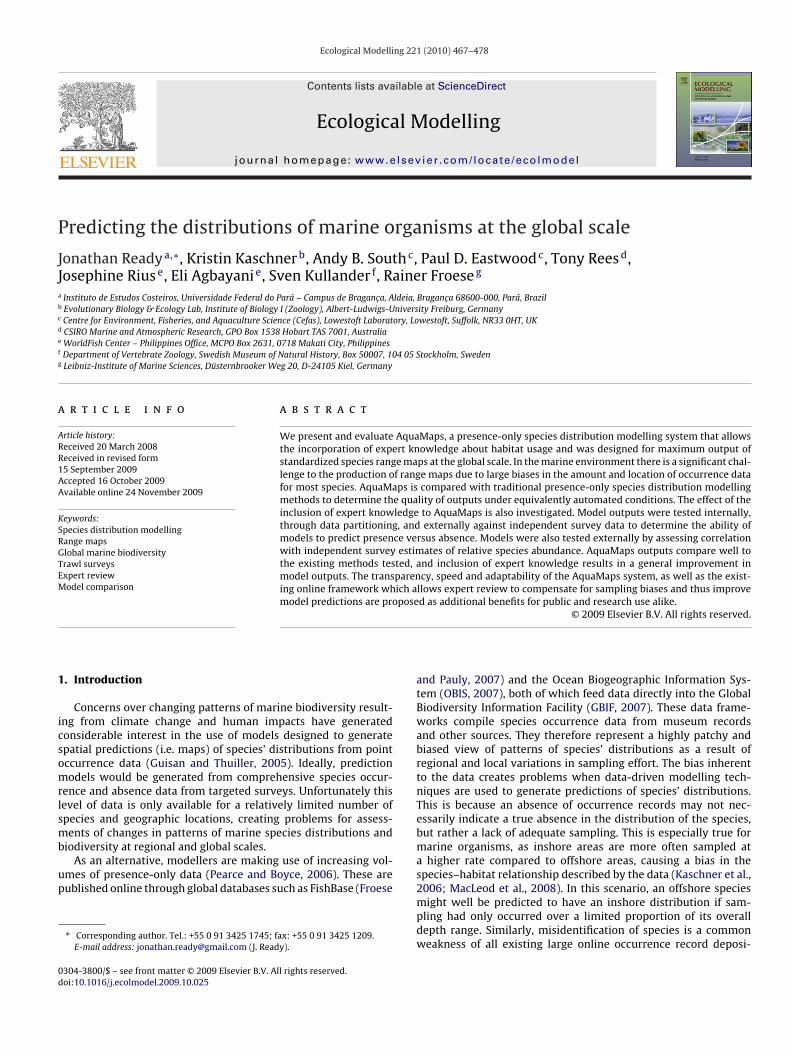
ted from pre-defined ‘environmental envelopes’ that numericallyescribe a species response to an environmental gradient basedn published information about species-specific habitat usage.he combination of these responses in every cell determines theuitability of that cell for the species. Similarly to the RES mod-lling approach AquaMaps relies on a pre-defined, trapezoidalhape (Fig. 1 here and Figs. 2 and 5 of Kaschner et al., 2006)o describe the basic relationship between species occurrence by

eans of a preferred range and an absolute range representinghe limits of tolerance with respect to a set of equally pre-definednvironmental predictors. In addition, AquaMaps does not gohrough an iterative model selection process which allows foron-linear complex interactions between different predictors, butomputes overall probabilities using a simple generic multiplica-ive model (see below). Hardwiring of the shape of environmentalnvelopes, predictor selection and model definition was used toa) maximize transparency and facilitate intuitive understandingf species response curves and predictor interactions for non-odellers (a pre-requisite for expert review and identification

f sampling biases), (b) speed up computational processing, andc) maintain clarity in the reproducibility of the results (using

he same envelopes, algorithm and environmental data, any GISr database system should be able to produce the same out-ut).

Anchor points for the species-specific absolute and preferredabitat ranges (i.e. environmental envelopes) are calculated based

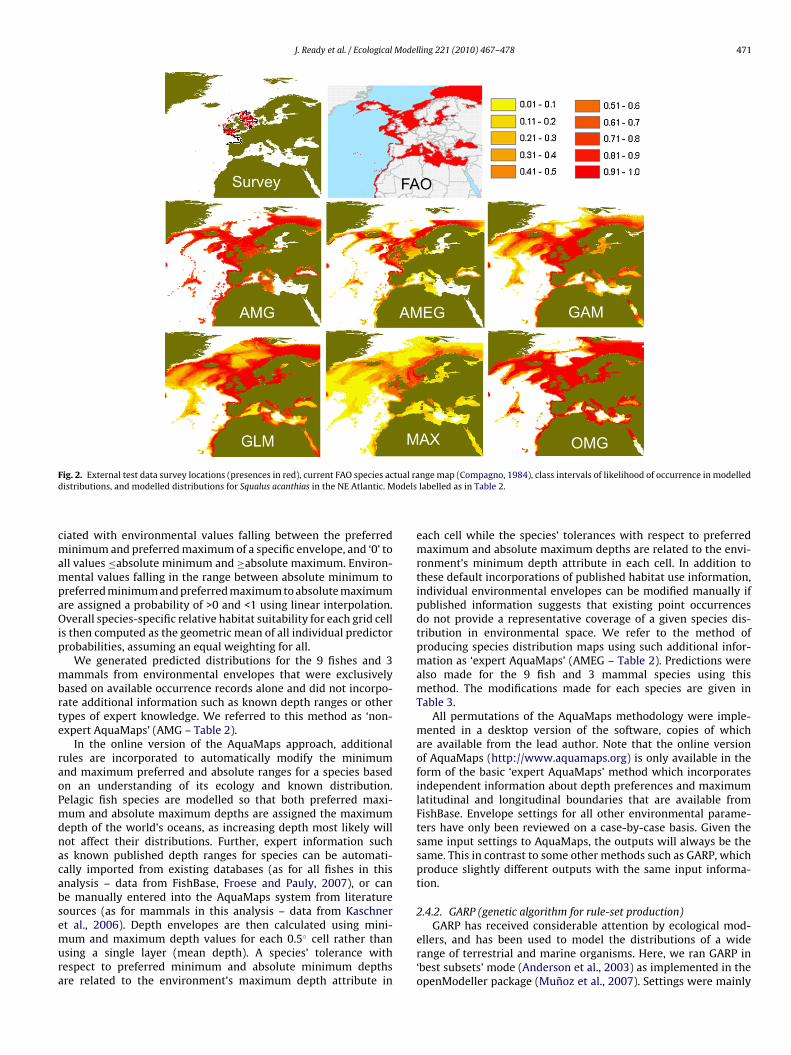
ig. 1. Comparison of the envelopes of AquaMaps (AMG and AMEG) with the response culasses of the environmental variable. Envelopes or response curves for depth and sea surSQACA and ZEFAB).

istical software http://cran.r-project.org/istical software http://cran.r-project.org/nt http://www.cs.princeton.edu/∼schapire/maxent/Modeller http://openmodeller.sourceforge.net/

on a subset of available presence cells that have been subjectedto a series of location-based quality checks (see above). The envi-ronmental envelopes are computed from the environmental valuesof the locations at which the species is found to occur using thefollowing rules:

• Absolute minimum (MinA) = the 25th percentile of the environ-mental values − (1.5 × the interquartile range), OR the absoluteminimum environmental value at which the species is observed,whichever is lower

• Preferred minimum (MinP) = the 10th percentile of the environ-mental values

• Preferred maximum (MaxP) = the 90th percentile of the environ-mental values

• Absolute maximum (MaxA) = the 75th percentile of the environ-mental values + (1.5 × the interquartile range), OR the absolutemaximum environmental value at which the species is observed,whichever is greater

Computed environmental envelopes for each species canbe viewed alongside their maps online through http://www.

aquamaps.org with some examples shown in Fig. 1, while valuesfor maxima and minima for all species in this analysis are describedin Table 3. After the definition of environmental envelopes, predic-tions of species-specific relative habitat suitability are generated foreach 0.5◦ grid cell by assigning a probability of ‘1’ to all cells asso-

rves generated by Maxent. Histograms represent frequencies of presence points forface temperature are shown for one mammal species (HYPLA) and two fish species

J. Ready et al. / Ecological Modelling 221 (2010) 467–478 471

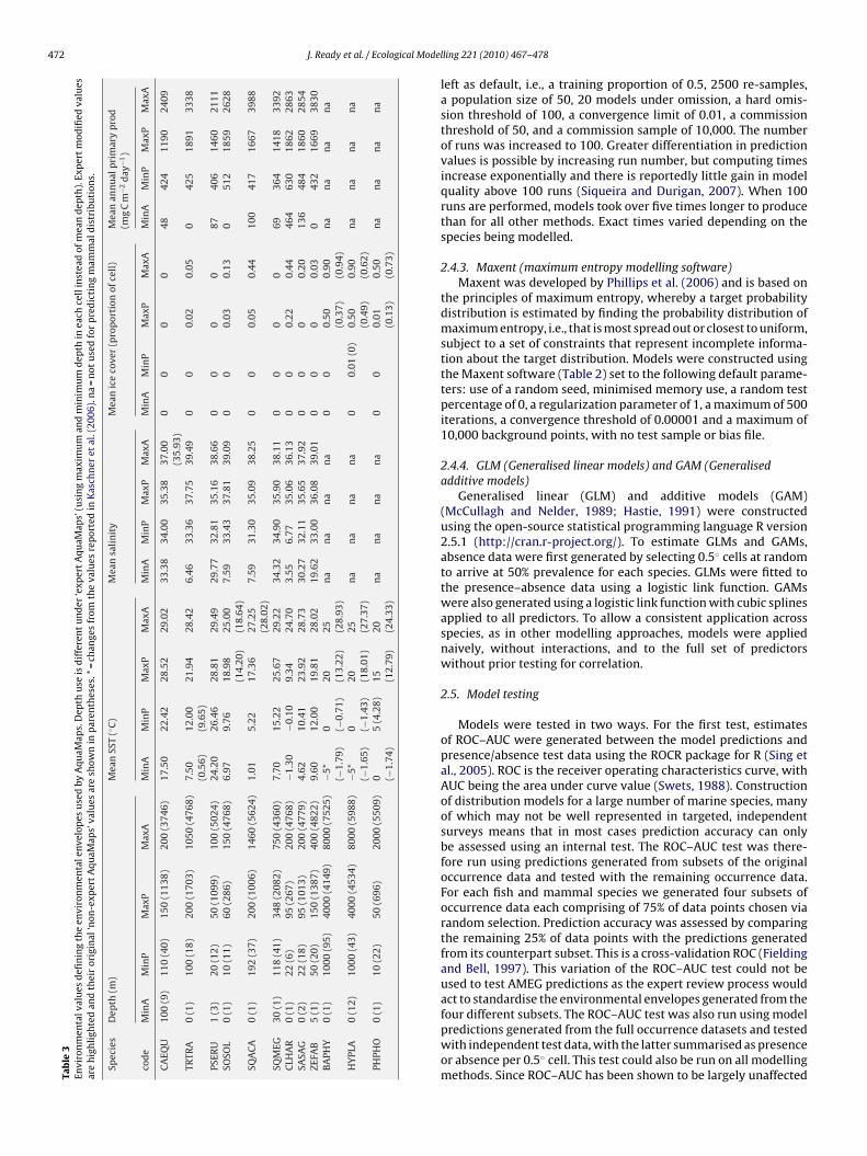
F tual rad odels

cmampaOip

mbrte

raoPmdnacabsemura

ig. 2. External test data survey locations (presences in red), current FAO species acistributions, and modelled distributions for Squalus acanthias in the NE Atlantic. M

iated with environmental values falling between the preferredinimum and preferred maximum of a specific envelope, and ‘0’ to

ll values ≤absolute minimum and ≥absolute maximum. Environ-ental values falling in the range between absolute minimum to

referred minimum and preferred maximum to absolute maximumre assigned a probability of >0 and <1 using linear interpolation.verall species-specific relative habitat suitability for each grid cell

s then computed as the geometric mean of all individual predictorrobabilities, assuming an equal weighting for all.

We generated predicted distributions for the 9 fishes and 3ammals from environmental envelopes that were exclusively

ased on available occurrence records alone and did not incorpo-ate additional information such as known depth ranges or otherypes of expert knowledge. We referred to this method as ‘non-xpert AquaMaps’ (AMG – Table 2).

In the online version of the AquaMaps approach, additionalules are incorporated to automatically modify the minimumnd maximum preferred and absolute ranges for a species basedn an understanding of its ecology and known distribution.elagic fish species are modelled so that both preferred maxi-um and absolute maximum depths are assigned the maximum

epth of the world’s oceans, as increasing depth most likely willot affect their distributions. Further, expert information suchs known published depth ranges for species can be automati-ally imported from existing databases (as for all fishes in thisnalysis – data from FishBase, Froese and Pauly, 2007), or cane manually entered into the AquaMaps system from literatureources (as for mammals in this analysis – data from Kaschner

t al., 2006). Depth envelopes are then calculated using mini-um and maximum depth values for each 0.5◦ cell rather than

sing a single layer (mean depth). A species’ tolerance withespect to preferred minimum and absolute minimum depthsre related to the environment’s maximum depth attribute in

nge map (Compagno, 1984), class intervals of likelihood of occurrence in modelledlabelled as in Table 2.

each cell while the species’ tolerances with respect to preferredmaximum and absolute maximum depths are related to the envi-ronment’s minimum depth attribute in each cell. In addition tothese default incorporations of published habitat use information,individual environmental envelopes can be modified manually ifpublished information suggests that existing point occurrencesdo not provide a representative coverage of a given species dis-tribution in environmental space. We refer to the method ofproducing species distribution maps using such additional infor-mation as ‘expert AquaMaps’ (AMEG – Table 2). Predictions werealso made for the 9 fish and 3 mammal species using thismethod. The modifications made for each species are given inTable 3.

All permutations of the AquaMaps methodology were imple-mented in a desktop version of the software, copies of whichare available from the lead author. Note that the online versionof AquaMaps (http://www.aquamaps.org) is only available in theform of the basic ‘expert AquaMaps’ method which incorporatesindependent information about depth preferences and maximumlatitudinal and longitudinal boundaries that are available fromFishBase. Envelope settings for all other environmental parame-ters have only been reviewed on a case-by-case basis. Given thesame input settings to AquaMaps, the outputs will always be thesame. This in contrast to some other methods such as GARP, whichproduce slightly different outputs with the same input informa-tion.

2.4.2. GARP (genetic algorithm for rule-set production)

GARP has received considerable attention by ecological mod-

ellers, and has been used to model the distributions of a widerange of terrestrial and marine organisms. Here, we ran GARP in‘best subsets’ mode (Anderson et al., 2003) as implemented in theopenModeller package (Munoz et al., 2007). Settings were mainly

472 J. Ready et al. / Ecological ModelTa

ble

3En

viro

nm

enta

lval

ues

defi

nin

gth

een

viro

nm

enta

len

velo

pes

use

dby

Aqu

aMap

s.D

epth

use

isd

iffe

ren

tu

nd

er‘e

xper

tA

quaM

aps’

(usi

ng

max

imu

man

dm

inim

um

dep

thin

each

cell

inst

ead

ofm

ean

dep

th).

Exp

ert

mod

ified

valu

esar

eh

igh

ligh

ted

and

thei

ror

igin

al‘n

on-e

xper

tA

quaM

aps’

valu

esar

esh

own

inp

aren

thes

es.*

=ch

ange

sfr

omth

eva

lues

rep

orte

din

Kas

chn

eret

al.(

2006

).n

a=

not

use

dfo

rp

red

icti

ng

mam

mal

dis

trib

uti

ons.

Spec

ies

Dep

th(m

)M

ean

SST

(◦ C)

Mea

nsa

lin

ity

Mea

nic

eco

ver

(pro

por

tion

ofce

ll)

Mea

nan

nu

alp

rim

ary

pro

d(m

gC

m−2

day

−1)

cod

eM

inA

Min

PM

axP

Max

AM

inA

Min

PM

axP

Max

AM

inA

Min

PM

axP

Max

AM

inA

Min

PM

axP

Max

AM

inA

Min

PM

axP

Max

A

CA

EQU

100

(9)

110

(40)

150

(113

8)20

0(3

746)

17.5

022

.42

28.5

229

.02

33.3

834

.00

35.3

837

.00

(35.

93)

00

00

4842

411

9024

09

TRTR

A0

(1)

100

(18)

200

(170

3)10

50(4

768)

7.50

(0.5

6)12

.00

(9.6

5)21

.94

28.4

26.

4633

.36

37.7

539

.49

00

0.02

0.05

042

518

9133

38

PSER

U1

(3)

20(1

2)50

(109

9)10

0(5

024)

24.2

026

.46

28.8

129

.49

29.7

732

.81

35.1

638

.66

00

00

8740

614

6021

11SO

SOL

0(1

)10

(11)

60(2

86)

150

(476

8)6.

979.

7618

.98

(14.

20)

25.0

0(1

8.64

)7.

5933

.43

37.8

139

.09

00

0.03

0.13

051

218

5926

28

SQA

CA

0(1

)19

2(3

7)20

0(1

006)

1460

(562

4)1.

015.

2217

.36

27.2

5(2

8.02

)7.

5931

.30

35.0

938

.25

00

0.05

0.44

100

417

1667

3988

SQM

EG30

(1)

118

(41)

348

(208

2)75

0(4

360)

7.70

15.2

225

.67

29.2

234

.32

34.9

035

.90

38.1

10

00

069

364

1418

3392

CLH

AR

0(1

)22

(6)

95(2

67)

200

(476

8)−1

.30

−0.1

09.

3424

.70

3.55

6.77

35.0

636

.13

00

0.22

0.44

464

630

1862

2863

SASA

G0

(2)

22(1

8)95

(101

3)20

0(4

779)

4.62

10.4

123

.92

28.7

330

.27

32.1

135

.65

37.9

20

00

0.20

136

484

1860

2854

ZEFA

B5

(1)

50(2

0)15

0(1

387)

400

(482

2)9.

6012

.00

19.8

128

.02

19.6

233

.00

36.0

839

.01

00

00.

030

432

1669

3830

BA

PHY

0(1

)10

00(9

5)40

00(4

149)

8000

(752

5)−5

*(−

1.79

)0 (−

0.71

)20 (1

3.22

)25 (2

8.93

)n

an

an

an

a0

00.

50(0

.37)

0.90

(0.9

4)n

an

an

an

a

HY

PLA

0(1

2)10

00(4

3)40

00(4

534)

8000

(598

8)−5

*(−

1.65

)0 (−

1.43

)20 (1

8.01

)25 (2

7.37

)n

an

an

an

a0

0.01

(0)

0.50

(0.4

9)0.

90(0

.62)

na

na

na

na

PHPH

O0

(1)

10(2

2)50

(696

)20

00(5

509)

0 (−1.

74)

5(4

.28)

15 (12.

79)

20 (24.

33)

na

na

na

na

00

0.01

(0.1

3)0.

50(0

.73)

na

na

na

na

ling 221 (2010) 467–478

left as default, i.e., a training proportion of 0.5, 2500 re-samples,a population size of 50, 20 models under omission, a hard omis-sion threshold of 100, a convergence limit of 0.01, a commissionthreshold of 50, and a commission sample of 10,000. The numberof runs was increased to 100. Greater differentiation in predictionvalues is possible by increasing run number, but computing timesincrease exponentially and there is reportedly little gain in modelquality above 100 runs (Siqueira and Durigan, 2007). When 100runs are performed, models took over five times longer to producethan for all other methods. Exact times varied depending on thespecies being modelled.

2.4.3. Maxent (maximum entropy modelling software)Maxent was developed by Phillips et al. (2006) and is based on

the principles of maximum entropy, whereby a target probabilitydistribution is estimated by finding the probability distribution ofmaximum entropy, i.e., that is most spread out or closest to uniform,subject to a set of constraints that represent incomplete informa-tion about the target distribution. Models were constructed usingthe Maxent software (Table 2) set to the following default parame-ters: use of a random seed, minimised memory use, a random testpercentage of 0, a regularization parameter of 1, a maximum of 500iterations, a convergence threshold of 0.00001 and a maximum of10,000 background points, with no test sample or bias file.

2.4.4. GLM (Generalised linear models) and GAM (Generalisedadditive models)

Generalised linear (GLM) and additive models (GAM)(McCullagh and Nelder, 1989; Hastie, 1991) were constructedusing the open-source statistical programming language R version2.5.1 (http://cran.r-project.org/). To estimate GLMs and GAMs,absence data were first generated by selecting 0.5◦ cells at randomto arrive at 50% prevalence for each species. GLMs were fitted tothe presence–absence data using a logistic link function. GAMswere also generated using a logistic link function with cubic splinesapplied to all predictors. To allow a consistent application acrossspecies, as in other modelling approaches, models were appliednaively, without interactions, and to the full set of predictorswithout prior testing for correlation.

2.5. Model testing

Models were tested in two ways. For the first test, estimatesof ROC–AUC were generated between the model predictions andpresence/absence test data using the ROCR package for R (Sing etal., 2005). ROC is the receiver operating characteristics curve, withAUC being the area under curve value (Swets, 1988). Constructionof distribution models for a large number of marine species, manyof which may not be well represented in targeted, independentsurveys means that in most cases prediction accuracy can onlybe assessed using an internal test. The ROC–AUC test was there-fore run using predictions generated from subsets of the originaloccurrence data and tested with the remaining occurrence data.For each fish and mammal species we generated four subsets ofoccurrence data each comprising of 75% of data points chosen viarandom selection. Prediction accuracy was assessed by comparingthe remaining 25% of data points with the predictions generatedfrom its counterpart subset. This is a cross-validation ROC (Fieldingand Bell, 1997). This variation of the ROC–AUC test could not beused to test AMEG predictions as the expert review process wouldact to standardise the environmental envelopes generated from the

four different subsets. The ROC–AUC test was also run using modelpredictions generated from the full occurrence datasets and testedwith independent test data, with the latter summarised as presenceor absence per 0.5◦ cell. This test could also be run on all modellingmethods. Since ROC–AUC has been shown to be largely unaffected

J. Ready et al. / Ecological Modelling 221 (2010) 467–478 473

F acrossd erformi

bd

omirftracpridfd

3

f

ig. 3. ROC–AUC internal test results show variation between modelling methodsifferent 75% subsets of the original occurrence data for each species. No test was p

n Table 1 and ordered left to right based on increasing training data sample size.

y species prevalence, it allows a direct comparisons of models forifferent species (McPherson et al., 2004).

The second test was used to assess to what extent predictionsf relative habitat suitability produced by the different modelsatched observed indices of effort-corrected species occurrence.

.e. to compare gradients of predicted and observed species occur-ence. The test we used was developed by Kaschner et al. (2006)ollowing an approach recommended by Pearce and Boyce (2006)o test predictions of presence-only models. Spearman’s rank cor-elations are computed between model predictions and relativebundance/density estimates based on the average effort-correctedatch or sighting rates over all cells within classes of predictedrobability. To assess the performance of our models compared toandom distributions, we obtained a simulated p-value by record-ng the number of times the relationship between 1000 randomata sets and test data sets was as strong as or stronger than thatound between the observed encounter rates and the model pre-ictions.

. Results

The various model algorithms generated different predictionsor each species, and the envelopes and response curves for some

the range of input data quantity and species. Model predictions are based on foured for AMEG as expert adaption results in a single output. Species are labelled as

of these are presented for comparison in Fig. 1. Fig. 2 shows themodel outputs for Squalus acanthias along with the survey datacollection locations used for external testing of the models and thecurrent FAO distribution map for the same species in the same area(Compagno, 1984). In all cases the models predicted S. acanthias tooccur far beyond the geographic range described by the input data.The AMG model describes a similar pattern to the known distribu-tion, though with some restriction of range in areas of extremelyhigh and low salinity (Mediterranean, Red and Baltic seas). TheAMEG model is similar in overall extent (area) but shows a signif-icant restriction in probabilities with depth. The difference in thisrespect is clearly seen in the expert modifications for depth acrossall species (Table 3 and Fig. 1). The GAM model is quite similar tothe AMG model, though indicates a greater proportion of less suit-able environments. The GLM and MAX models cover a greater rangethan the other models, with the difference between them being thatthe GLM model predicts a relatively large proportion of the rangeas having a high probability of occurrence while the MAX model

predicts only a small proportion of the overall range will have ahigh probability of occurrence. The OMG model predicts much thesame range as the GAM model, though it predicts nearly all of therange to have a high likelihood of occurrence, with variation in like-lihood of occurrence being restricted to the peripheral areas of the

474 J. Ready et al. / Ecological Model

Far

raotome

sdbeddvaclaZgrfi(nop4

c(tmb(mwsmp

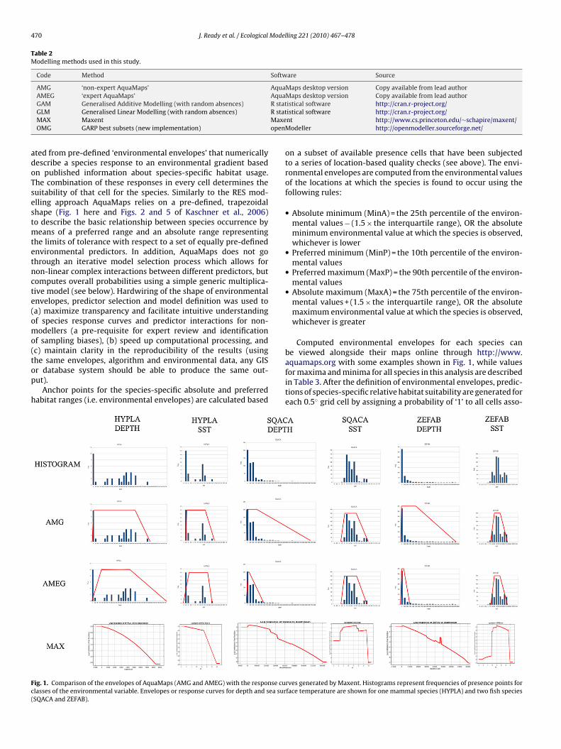
which correlate with survey abundances. GLM predictions showeda similar trend but performed less successfully overall. Maxentmodels performed successfully for a similar number of species asAMG though for a slightly different set of species, and OMG predic-tions performed poorly.

ig. 4. ROC–AUC statistical results for model predictions based on all points testedgainst external survey data Species are labelled as in Table 1 and ordered left toight based on increasing training data sample size.

ange. The variation between model predictions in terms of rangend the proportion of the range predicted to have a high likelihoodf occurrence is generally similar for the other species. The excep-ions are AMEG models where, apart from similar changes basedn use of maximum and minimum depths (Table 3), variation isore dependent on the degree of changes due to expert modified

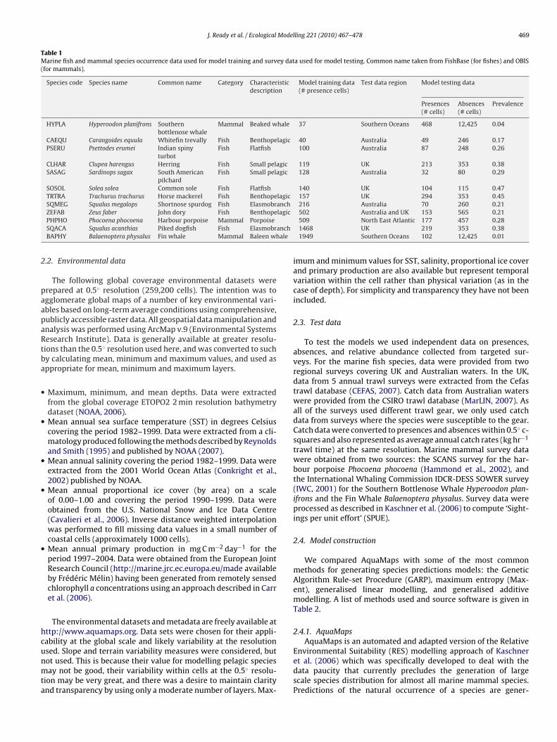
nvelopes.Internal testing of predictions using ROC–AUC scores for four

ubsets testing against remaining non-independent occurrenceata (Fig. 3) showed that modelling methods generally providedetter outputs for species with more data (as seen for some mod-ls where results are poor using the lowest numbers of trainingata). Deviations from this trend with large amounts of trainingata indicate points of note. ROC–AUC scores are lower and moreariable with subsets of 37/40 occurrence points and generally highnd not as variable with subsets of 100+ occurrence points. Thelear exception is for B. physalus which generally performed slightlyess well than might be expected for all models given the largemount of training data. Trachurus trachurus, Sardinops sagax and. faber also showed scores that were marginally lower than theeneral trend. When comparing different models, the GAMs obtainemarkably high scores with little variation. Exceptions to this areor the taxa Squalus megalops and Z. faber, where the distinct dropn ROC–AUC scores is consistent with a limited number of classes2) generated by the GAM model predicted distribution. The lowumber of classes of outputs also explains the non-valid resultsf Spearman’s rank test for these taxa when this model is com-ared with the species survey abundance estimates (see Section).

External testing through calculation of ROC–AUC scores fromomparison of predictions with external independent test dataFig. 4) are very variable and generally not very high, even whenraining data quantity is maximised. Some species appear to be

odelled well at least by some modelling methods (comparativelyetter ROC–AUC values). Comparatively better ROC-AUC scores>0.7) were obtained for Carangoides equula, Clupea harengus, S.

egalops and Z. faber models produced by both AMG and AMEGhile MAX models of C. harengus, S. megalops and Z. faber also

cored comparatively well. GLMs produced comparatively goododels for C. harengus and S. sagax, while GAM and OMG methods

roduced no models gaining such ROC–AUC scores.

ling 221 (2010) 467–478

External testing comparing relative predicted probabilities withrelative abundances of species from survey data varied in asimilar way to ROC–AUC scores in most respects with good cor-relations possible when models are made from as little as 37occurrence points (Table 4 and Fig. 5). Overall, models tended toperform better in terms of predicting gradients of relative speciesoccurrence as indicated by the higher number of statisticallysignificant correlations with external survey data. Interestingly,GAMs, which performed extremely poorly in terms of predict-ing binary presence/absence of species, was one of the methodsable to predict relative species occurrence most reliably. OMGmodels again performed poorly. Again, the low number of out-put classes produced from these models made some comparisons(four species) statistically impossible. It should be noted that therewas no significant result for OMG models of C. harengus and B.physalus, which were modelled well by almost all other meth-ods.

Expert review effects on predictions based on results in Table 4and Figs. 4 and 5 show that for most species for which AMG mod-els were good predictors, the main effect in ‘expert AquaMaps’ wasan improvement in ROC–AUC score or correlation with survey data,and that this is largely related to the incorporation of expert defineddepth preferences and the different use of depth data in AMEGwhere a species’ response to depth can be applied to both maxi-mum and minimum depths of a cell instead of just mean depth ofthe cell (Table 3).

A summary of the results of both ROC–AUC and Spearman’srank statistics gives model/species combinations which have botha good range as determined by the ROC–AUC score and a goodcorrelation with existing abundances (Table 5). Comparing modelmethod results, AMG predictions vary to some extent with species,but produce reasonable results under both testing methods andAMEG predictions performed generally slightly better than AMG.GAM predictions performed very poorly at prediction of presencevs. absence (ROC–AUC), but very well at producing predictions

Fig. 5. Results of Spearman’s rank correlation of predicted models with survey abun-dances (significant correlations highlighted in Table 4 have filled symbols). Speciesare labelled as in Table 1 and ordered left to right based on increasing training datasample size.

J. Ready et al. / Ecological Modelling 221 (2010) 467–478 475

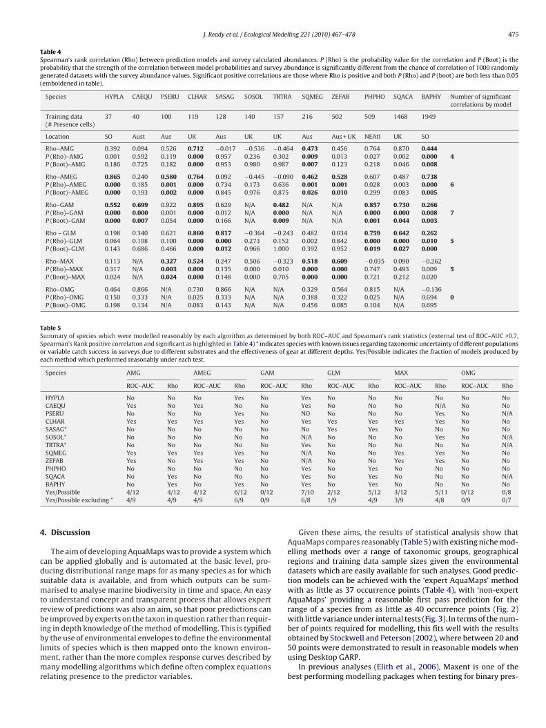
Table 4Spearman’s rank correlation (Rho) between prediction models and survey calculated abundances. P (Rho) is the probability value for the correlation and P (Boot) is theprobability that the strength of the correlation between model probabilities and survey abundance is significantly different from the chance of correlation of 1000 randomlygenerated datasets with the survey abundance values. Significant positive correlations are those where Rho is positive and both P (Rho) and P (boot) are both less than 0.05(emboldened in table).

Species HYPLA CAEQU PSERU CLHAR SASAG SOSOL TRTRA SQMEG ZEFAB PHPHO SQACA BAPHY Number of significantcorrelations by model

Training data(# Presence cells)

37 40 100 119 128 140 157 216 502 509 1468 1949

Location SO Aust Aus UK Aus UK UK Aus Aus + UK NEAtl UK SO

Rho–AMG 0.392 0.094 0.526 0.712 −0.017 −0.536 −0.464 0.473 0.456 0.764 0.870 0.444P (Rho)–AMG 0.001 0.592 0.119 0.000 0.957 0.236 0.302 0.009 0.013 0.027 0.002 0.000 4P (Boot)–AMG 0.186 0.725 0.182 0.000 0.953 0.980 0.987 0.007 0.123 0.218 0.046 0.008

Rho–AMEG 0.865 0.240 0.580 0.764 0.092 −0.445 −0.090 0.462 0.528 0.607 0.487 0.738P (Rho)–AMEG 0.000 0.185 0.001 0.000 0.734 0.173 0.636 0.001 0.001 0.028 0.003 0.000 6P (Boot)–AMEG 0.000 0.193 0.002 0.000 0.845 0.976 0.875 0.026 0.010 0.299 0.083 0.005

Rho–GAM 0.552 0.699 0.922 0.895 0.629 N/A 0.482 N/A N/A 0.857 0.730 0.266P (Rho)–GAM 0.000 0.000 0.001 0.000 0.012 N/A 0.000 N/A N/A 0.000 0.000 0.008 7P (Boot)–GAM 0.000 0.007 0.054 0.000 0.166 N/A 0.009 N/A N/A 0.001 0.044 0.003

Rho – GLM 0.198 0.340 0.621 0.860 0.817 −0.364 −0.243 0.482 0.034 0.759 0.642 0.262P (Rho)–GLM 0.064 0.198 0.100 0.000 0.000 0.273 0.152 0.002 0.842 0.000 0.000 0.010 5P (Boot)–GLM 0.143 0.686 0.466 0.000 0.012 0.966 1.000 0.392 0.952 0.019 0.027 0.000

Rho–MAX 0.113 N/A 0.327 0.524 0.247 0.506 −0.323 0.518 0.609 −0.035 0.090 −0.262P (Rho)–MAX 0.317 N/A 0.003 0.000 0.135 0.000 0.010 0.000 0.000 0.747 0.493 0.009 5P (Boot)–MAX 0.024 N/A 0.024 0.000 0.148 0.000 0.705 0.000 0.000 0.721 0.212 0.020

Rho–OMG 0.464 0.866 N/A 0.730 0.866 N/A N/A 0.329 0.564 0.815 N/A −0.136P (Rho)–OMG 0.150 0.333 N/A 0.025 0.333 N/A N/A 0.388 0.322 0.025 N/A 0.694 0P (Boot)–OMG 0.198 0.134 N/A 0.083 0.143 N/A N/A 0.456 0.085 0.104 N/A 0.695

Table 5Summary of species which were modelled reasonably by each algorithm as determined by both ROC–AUC and Spearman’s rank statistics (external test of ROC–AUC >0.7,Spearman’s Rank positive correlation and significant as highlighted in Table 4) * indicates species with known issues regarding taxonomic uncertainty of different populationsor variable catch success in surveys due to different substrates and the effectiveness of gear at different depths. Yes/Possible indicates the fraction of models produced byeach method which performed reasonably under each test.

Species AMG AMEG GAM GLM MAX OMG

ROC–AUC Rho ROC–AUC Rho ROC–AUC Rho ROC–AUC Rho ROC–AUC Rho ROC–AUC Rho

HYPLA No No No Yes No Yes No No No No No NoCAEQU Yes No Yes No No Yes No No No N/A No NoPSERU No No No Yes No NO No No No Yes No N/ACLHAR Yes Yes Yes Yes No Yes Yes Yes Yes Yes No NoSASAG* No No No No No No Yes Yes No No No NoSOSOL* No No No No No N/A No No No Yes No N/ATRTRA* No No No No No Yes No No No No No N/ASQMEG Yes Yes Yes Yes No N/A No No Yes Yes No NoZEFAB Yes No Yes Yes No N/A No No Yes Yes No NoPHPHO No No No No No Yes No Yes No No No NoSQACA No Yes No No No Yes No Yes No No No N/A

4

cdsmtrbiblmmr

BAPHY No Yes No Yes NoYes/Possible 4/12 4/12 4/12 6/12 0/12Yes/Possible excluding * 4/9 4/9 4/9 6/9 0/9

. Discussion

The aim of developing AquaMaps was to provide a system whichan be applied globally and is automated at the basic level, pro-ucing distributional range maps for as many species as for whichuitable data is available, and from which outputs can be sum-arised to analyse marine biodiversity in time and space. An easy

o understand concept and transparent process that allows experteview of predictions was also an aim, so that poor predictions cane improved by experts on the taxon in question rather than requir-

ng in depth knowledge of the method of modelling. This is typified

y the use of environmental envelopes to define the environmental

imits of species which is then mapped onto the known environ-ent, rather than the more complex response curves described byany modelling algorithms which define often complex equations

elating presence to the predictor variables.

Yes No Yes No No No No7/10 2/12 5/12 3/12 5/11 0/12 0/86/8 1/9 4/9 3/9 4/8 0/9 0/7

Given these aims, the results of statistical analysis show thatAquaMaps compares reasonably (Table 5) with existing niche mod-elling methods over a range of taxonomic groups, geographicalregions and training data sample sizes given the environmentaldatasets which are easily available for such analyses. Good predic-tion models can be achieved with the ‘expert AquaMaps’ methodwith as little as 37 occurrence points (Table 4), with ‘non-expertAquaMaps’ providing a reasonable first pass prediction for therange of a species from as little as 40 occurrence points (Fig. 2)with little variance under internal tests (Fig. 3). In terms of the num-ber of points required for modelling, this fits well with the results

obtained by Stockwell and Peterson (2002), where between 20 and50 points were demonstrated to result in reasonable models whenusing Desktop GARP.

In previous analyses (Elith et al., 2006), Maxent is one of thebest performing modelling packages when testing for binary pres-

4 Model

etpHthswa(assMri(ti2mst

(tsosf(cGtom

(tapsnwhorean

ttpWsistfwftAtd

76 J. Ready et al. / Ecological

nce/absence (ROC–AUC). Similar analyses performed here supporthis result to some extent, though Maxent models were found toerform poorly for some taxa (particularly the mammals – Fig. 3).owever, even when performing well under ROC–AUC analysis,

he degree of correlation with survey data was not necessarily theighest of the modelling methods used. C. harengus was the onlypecies for which almost all modelling methods produced modelsith statistically significant correlations with survey abundances,

nd yet the correlation value obtained by Maxent was the lowestTable 4). The only case in which Maxent was uniquely better thanll other models was for Solea solea (Tables 4 and 5). This is the onlypecies for which training data came almost exclusively from theame region as the independent survey dataset. This indicates thataxent may over-fit predictions to the areas where sample occur-

ence data have been collected. This may be especially true if theres some kind of sampling selection bias to these collection locationse.g. a preference to catch fish in shallower water of a certain bottomype). Maxent does have an ability to counteract over-fitting usingts regularization procedure (Hernandez et al., 2006; Phillips et al.,006), but it is unclear as to how this might be included in auto-ated mapping of many species. It would only be useful for some

pecies, and it may not be a valuable exercise given assumptionshat the sampling is not biased (Phillips, 2008).

GLMs and GAMs are commonly used to model distributionsGuisan and Thuiller, 2005), but rely on input in the analysiso obtain best results. Under the requirements of an automatedystem, where selection of variables is standardised, these meth-ds appear to perform poorly (Table 5). Neither performs well intandard binary presence/absence tests (ROC–AUC). The GAMs per-ormed relatively well in the tests of correlation with survey dataTables 4 and 5), although notably for species which other methodsould not model well. Of particular note was the correlation of theAM model for T. trachurus. This species may in fact represent more

han one species (see discussion below) and as such the productionf a model that performs well in such tests may not indicate goododel performance.OMG (GARP) models performed badly in almost all comparisons

Tables 4 and 5). The outputs were generally much more variablehan all other methods and only seemed to reduce in variabilitynd obtain a stable ROC–AUC score when over 1000 occurrenceoints were used to model the distribution, at which point thecores are quite low (Fig. 3). This is likely a result of the lowerumber of output classes under OMG models. This is seen in Fig. 2here the predicted area includes a uniform block of red with aigh predicted value (0.9–1). It is possible that a higher numberf output classes might be producible by increasing the number ofuns performed when modelling distributions using OMG. How-ver, this would require modelling time in excess of that availablend may not improve the output quality enough to generate theeeded classes.

As all models were developed with the same set of environmen-al layers, variation in statistical support for the models is expectedo vary with life history, taxonomic group/status and bias in sam-ling distribution. This is clearly seen in the statistical analysis.hen looking at internal tests with subsets of data (Fig. 2), the

lightly lower ROC–AUC score of Z. faber is likely due to the fact thatt lives over a greater range than all other fish species, and as suchample selection bias may be greater due to more data from bet-er sampled regions. Models for B. physalus show a significant droprom the trend based on numbers of occurrence points included,hich may in part be due to sample selection bias over a large range

or both sampling and surveying options, where both are limitedemporally (to different extents) to the Antarctic summer season.dditionally, samples from whaling efforts which are included in

he OBIS dataset may be biased to areas known for higher abun-ances of both this and other species. Modelling performance may

ling 221 (2010) 467–478

also be poor for specific species if taxonomic uncertainty leadsto the inclusion of environments to which different populations(potential taxa) are adapted. This may explain the poor modellingperformance for S. sagax and T. trachurus by almost all modellingsystems. S. sagax represents a species which has genetically identi-fied sub-populations in different parts of its distribution (Grant etal., 1998), while T. trachurus represents a species where misidenti-fications may occur in part of its range due to presence of a closelyrelated species (southern populations of T. trachurus may representTrachurus capensis) (Froese and Pauly, 2007).

S. solea is one of the species that is generally modelled badlywhen compared to survey data (Table 5), and likely reflects therelative catch of the species being more sensitive to local factorswithin the survey area itself or the methods used to sample thespecies. S. solea has specific bottom type requirements, especiallywith regards to depth and sediment type (Rogers, 1992). It is notalways caught evenly in surveys as the catch efficiency of the gear,which is dependent on the bottom contact of the trawl and fishingprotocols, also varies with depth, bottom substrate and topogra-phy. The latter refers to the process by which faster or deepertrawls tend to cause the net to jump up more frequently resultingin poorer catches of bottom dwelling fish. The slightly less ‘bot-tom associated’ (Froese and Pauly, 2007) flatfish Psettodes erumeiwas apparently modelled slightly better with the inclusion of depthranges in ‘expert AquaMaps’ resulting in a significant correlation ofthe model with survey abundances, and the general additive modelnearing significant correlation.

The comparison of the expert input in AquaMaps is generallyfavourable to the inclusion of expert knowledge, but some loss inperformance underlines that existing expert knowledge may notalways result in improved outputs and supports the sensitivity ofhabitat rating to expert opinion found in previous analysis (Johnsonand Gillingham, 2004). All existing data, including expert knowl-edge, is prone to bias. Even if it is assumed that all T. trachurusoccurrence data are valid identifications, bias in occurrence dataand/or expert knowledge can explain the poor model performance.Such bias may be sufficiently strong (large survey datasets includedfrom certain regions) to result in poor predictions of suitable habi-tat in other regions or may also be combined with species-specificphenomena such as tropical submergence (Ekman, 1967) whichmay also lead to bias in expert knowledge as expert knowledge isgenerally biased towards surface waters.

The better performance of the ‘non-expert AquaMaps’ com-pared to ‘expert AquaMaps’ for S. acanthias and P. phocoena issuggested to be a result of a bias in the treatment of depth. ForS. acanthias, the given expert value for preferred depth range islikely wrong. Textual descriptions of localities where the species iscaught indicate a lower value should be applied to preferred mini-mum depth. Preliminary analysis with such lower values producedpredictions more similar to the ‘non-expert AquaMaps’ model. Theresult for S. acanthias highlights how such analyses can draw atten-tion to possible errors in data presented in the literature and takenas the current state of knowledge. S. acanthias was selected forFig. 2 to highlight the importance of verification of expert knowl-edge. Alternatively, the need for expert knowledge applied to theSouthern Bottlenose Whale, Hyperoodon planifrons (HYPLA), is evi-dent in the differences in the depth envelopes of AMG and AMEG(Fig. 1 and Table 3). The species is one of the deep-diving beakedwhale species, known to predominantly occur almost entirely indeeper waters (Gowans, 2002; Kasamatsu et al., 2000; MacLeodand D’Amico, 2006). The large number of shallow water sighting of

the species reflects known sampling biases of heterogeneous sur-vey efforts in shallow waters and potential misidentifications, as allbeaked whales are highly inconspicuous and difficult to identify atsea. In addition, the stranding records, which generally representthe most common form of available occurrence records for most

Model

bto

faodmnapgeouttm

ptt

mtfitmaitvewoflptpeeaocomCspbpded

dcomgbrlt

J. Ready et al. / Ecological

eaked whale species, would have been allocated to coastal (ratherhan land) cells and thus would not have been successfully filteredut during the initial screening for erroneous species reports.

The ‘expert AquaMaps’ envelope for P. phocoena had been takenrom the previous work of Kaschner et al. (2006) which used aver-ge depths and had not been adjusted to the current algorithm’s usef minimum and maximum depths. As such the differential use ofepth in ‘expert AquaMaps’ has worsened the correlation betweenodel and survey data (at least within the survey area) while the

on-expert mode used occurrence points from roughly the samerea as the independent survey dataset to create the model, thusroducing a reasonably good approximation. Further expert reviewiven knowledge of the new use of depth values may allow recov-ry of a stronger, more significant correlation for P. phocoena. Bothther mammals actually show improvements in statistical supportnder the new ‘expert AquaMaps’ prediction when compared tohe original RES model of Kaschner et al. (2006), indicating thathe method has generally remained effective for the prediction of

arine mammal distributions.If taxa with known issues regarding taxonomic uncertainty or

oor catch in survey are excluded from the summary in Table 5,hen the ‘expert AquaMaps’ also compares well with general addi-ive models under tests of correlation with survey abundance.

Lobo et al. (2008) argue that ROC–AUC scores are not a goodeasure of model performance for five reasons, one of which is that

hey ignore the predicted probability values and the goodness-of-t of the model. We use the Spearman’s rank statistic to directlyest for a good fit between the probability values generated by

odels and true abundances. The limitation of tests such as thisre that they require external survey data for the species stud-ed, including sampling from areas where abundances are lower,o confirm this goodness of fit. Such data are not available for theast majority of species. Lobo et al. (2008) also state that the totalxtent to which models are carried out highly influences the rate ofell-predicted absences and the AUC scores, with the generation

f pseudo-absences for points which are geographically and there-ore probably more environmentally distant from the presenceocalities leading to a low commission error. The statistical com-arisons carried out here were based on surveyed regions wherehe species modelled are known to occur, therefore avoiding thisroblem. Nevertheless ROC–AUC scores have been widely used incological modelling and retain some advantageous features. Lobot al. (2008) suggest that ‘the real value of AUC is that it providesmeasure of the degree to which a species is restricted to a part

f the variation range of the modelled predictors, so that presencesan be told apart from absences’ i.e. it tells us whether the rangef the predicted distribution is more or less accurate in environ-ental space, but not whether the internal probabilities are good.

omparison of ROC–AUC results of different models for the samepecies is possible because the data used to generate and test theredictions remain constant. ROC–AUC also remains useful as aasic statistic to determine the amount of variation in results fromartitioned datasets, as performed here, highlighting the potentialegree of sampling bias in the original datasets with respect to thenvironmental parameters used for modelling and the number andistribution of known occurrences used to generate the model.

Expert review remains the quickest way to improve predictedistributions in AquaMaps, but relies on expert knowledge being asomplete as possible. Taxonomic uncertainty and poor knowledgef biodiversity in certain geographical areas remain an impedi-ent to this. One of the main problems in modelling species at the

lobal scale is the failure to predict presence of species in enclosedays/seas where environmental conditions are distinct from sur-ounding areas (e.g. Red Sea, Baltic Sea and Arafura Sea). If speciesack records from such areas then their distributions often reflecthis with a predicted absence from the area. Expert review can read-

ling 221 (2010) 467–478 477

ily identify these cases and includes various methods for alteringspecies distributions to include these areas.

It will remain the case that an expert in modelling methodsshould be able to produce a better species distribution model by:using more data (presence and absence or even abundance); usingmore exhaustive methods (such as Boosted Regression Trees);applying better specific model settings (e.g. regularization in Max-ent); testing for and applying corrections to environmental biasin sampling, and; using more or different environmental layers(potentially at different resolutions) depending on the scale of theanalysis. However, such analyses must be made on a case-by-casebasis and require good knowledge of both the modelling methodsand the species biology, whereas if the aim is to summarise biodi-versity generally and quickly (Balmford et al., 2005), species rangemaps must be produced in the greatest possible number and usinga generalised method to maintain consistency. With the datasetsavailable at this time, AquaMaps provides such maps online fora large number of species and to a quality comparable to, if notbetter than, other methods tested here. In addition it provides theflexibility to review, adapt and store ranges online in a matter ofminutes which, as all predictions are in a single system, can thenbe summarised based on any number of criteria.

Acknowledgements

This work was supported in part by the European Commis-sion under the INCOFISH project (http://www.incofish.org), ECINCO contract no. 003739 and in part by Pew Grant UM2004-001034/PFP(NEA)03-01. P. Eastwood and A. South receivedadditional support from the UK Department for Environment, Food,and Rural Affairs through contract AE0916. We thank C. Close atthe University of British Columbia for assistance with the prepa-ration of environmental datasets, C. Allison and the Secretariat ofthe International Whaling Commission for providing us with theIWC catch and sighting datasets, and P. Hammond, Sea MammalResearch Unit, for the SCANS dataset.

References

Anderson, R.P., Lew, D., Peterson, A.T., 2003. Evaluating predictive models of species’distributions: criteria for selecting optimal models. Ecol. Model. 162, 211–232,doi:10.1016/S0304-3800(02)00349-6.

Balmford, A., Bennun, L., ten Brink, B., Cooper, D., Côté, I.M., Crane, P., Dobson, A.,Dudley, N., Dutton, I., Green, R.E., Gregory, R.D., Harrison, J., Kennedy, E.T., Kre-men, C., Leader-Williams, N., Lovejoy, T.E., Mace, G., May, R., Mayaux, P., Morling,P., Phillips, J., Redford, K., Ricketts, T.H., Rodríguez, J.P., Sanjayan, M., Schei, P.J.,van Jaarsveld, A.S., Walther, B.A., 2005. The convention on biological diversity’s2010 target. Science 307, 212–213, doi:10.1126/science.1106281.

Carr, M.-E., Friedrichs, A.M., Schmeltz, M., Aita, M.N., Antoine, D., Arrigo, K.R.,Asanuma, I., Aumont, O., Barber, R., Behrenfeld, M., Bidigare, R., Buitenhuis, E.T.,Campbell, J., Ciotti, A., Dierssen, H., Dowell, M., Dunne, J., Esaias, W., Gentili, B.,Gregg, W., Groom, S., Hoepffner, N., Ishizaka, J., Kameda, T., Le Quéré, C., Lohrenz,S., Marra, J., Mélin, F., Moore, K., Morel, A., Reddy, T.E., Ryan, J., Scardi, M., Smyth,T., Turpie, K., Tilstone, G., Waters, K., Yamanaka, Y., 2006. A comparison of globalestimates of marine primary production from ocean color. Deep-Sea Res., II 53,741–770.

Cavalieri, D., Parkinson, C., Gloersen, P., Zwally. H.J., 1996 (updated 2006). Sea iceconcentrations from Nimbus-7 SMMR and DMSP SSM/I passive microwave data,[1979–2002]. Boulder, Colorado USA: National Snow and Ice Data Center. Digitalmedia.

CEFAS, 2007. Centre for Environment, Fisheries & Aquaculture Sci-ence (Cefas) Web service. Data, Fisheries Information, Surveyshttp://www.cefas.co.uk/data/fisheries-information/surveys.aspx. AccessedDecember 2007.

Compagno, L.J.V., 1984. FAO species catalogue Vol.4. Sharks of the world. An Anno-tated and Illustrated Catalogue of Shark Species Known to Date Part 1 –Hexanchiformes to Lamniformes. FAO Fish. Synop., 125, Part 1.

Conkright, M.E., Locarnini, R.A., Garcia, H.E., O’Brien, T.D., Boyer, T.P., Stephens, C.,Antonov, J.I., 2002. World Ocean Atlas 2001: objective analyses, data statistics,and figures CD-ROM documentation. U.S. National Oceanographic and Atmo-spheric Administration, National Oceanographic Data Center, Silver Spring, MD,p. 17.

Ekman, S., 1967. Zoogeography of the Sea. Sidgwick & Jackson, London.

4 Model

E

F

F

G

G

G

G

H

H

H

I

J

K

K

L

M

M

lenhosas de cerrado no Estado de São Paulo. Revista Brasileira de Botânica 30,

78 J. Ready et al. / Ecological

lith, J., Graham, C.H., Anderson, R.P., Dudik, M., Ferrier, S., Guisan, A., Hijmans, R.J.,Huettmann, F., Leathwick, J.R., Lehmann, A., Li, J., Lohmann, L.G., Loiselle, B.A.,Manion, G., Moritz, C., Nakamura, M., Nakazawa, Y., Overton, J.Mc.C., Peterson,A.T., Phillips, S.J., Richardson, K., Scachetti-Pereira, R., Schapire, R.E., Soberón, J.,Williams, S., Wisz, M.S., Zimmermann, N.E., 2006. Novel methods improve pre-diction of species’ distributions from occurrence data. Ecography 29, 129–151.

ielding, A.H., Bell, J.F., 1997. A review of methods for the assessment of predictionerrors in conservation presence/absence models. Env. Cons. 24 (1), 38–49.

roese, R., Pauly, D., 2007. FishBase. World Wide Web electronic publication.http://www.fishbase.org. Version 01/2007.

BIF, 2007. Global Biodiversity Information Facility. World Wide Web electronicpublication http://www.gbif.org/. Accessed December 2007.

owans, S., 2002. Bottlenose Whales - Hyperoodon ampullus and H. planifrons. In: Per-rin, W.F., Würsig, B., Thewissen, J.G.M. (Eds.), Encyclopedia of Marine Mammals.Academic Press, San Diego, CA, pp. 128–129.

rant, W.S., Clark, A.M., Bowen, B.W., 1998. Why restriction fragment length poly-morphism analysis of mitochondrial DNA failed to resolve sardine (Sardinops)biogeography: insights from mitochondrial DNA cytochrome b sequences. Can.J. Fish Aquat. Sci. 55 (12), 2539–2547.

uisan, A., Thuiller, W., 2005. Predicting species distribution: offering more thansimple habitat models. Ecol. Lett. 8, 993–1009.

ammond, P.S., Berggren, P., Benke, H., Borchers, D.L., Collet, A., Heide-Jorgensen,M.P., Heimlich, S., Hiby, A.R., Leopold, M.F., Øien, N., 2002. Abundance of harbourporpoise and other cetaceans in the North Sea and adjacent waters. J. Appl. Ecol.39, 361–376.

astie, T.J., 1991. Generalized additive models. In: Chambers, J.M., Hastie, T.J. (Eds.),Statistical Models. S, Wadsworth & Brooks/Cole, Chapter 7.

ernandez, P.A., Graham, C.H., Máster, L.L., Albert, D.L., 2006. The effect of samplesize and species characteristics on performance of different species distributionmodelling methods. Ecography 29, 773–785.

WC (International Whaling Commission), 2001. IDCR-DESS SOWER survey data set(1978-2001). IWC, Cambridge.

ohnson, C.J., Gillingham, M.P., 2004. Mapping uncertainty: sensitivity of wildlifehabitat ratings to expert opinion. J. Appl. Ecol. 41, 1032–1041.

asamatsu, F., Matsuoka, K., Hakamada, T., 2000. Interspecific relationships in den-sity among the whale community in the Antarctic. Polar Biol. 23, 466–473.

aschner, K., Watson, R., Trites, A.W., Pauly, D., 2006. Mapping world wide distri-butions of marine mammal species using a relative environmental suitability(RES) model. MEPS 316, 285–310.

obo, J.M., Jiménez-Valverde, A., Real, R., 2008. AUC: a misleading measure of the per-formance of predictive distribution models. Global Ecol. Biogeogr. 17, 145–151.

acLeod, C.D., D’Amico, A., 2006. A review of beaked whale behaviour and ecology inrelation to assessing and mitigating impacts of anthropogenic noise. J. CetaceanRes. Manage. 7, 211–221.

acLeod, C.D., Mandleberg, L., Schweder, C., Bannon, S.M., Pierce, G.J., 2008. Acomparison of approaches for modelling the occurrence of marine animals.Hydrobiologia 612, 21–32, doi:10.1007/s10750-008-9491-0.

ling 221 (2010) 467–478

MarLIN, 2007. CSIRO Marine and Atmospheric Research (CMAR) LaboratoriesInformation Network http://www.marine.csiro.au/marlin/Accessed December2007.

McCullagh, P., Nelder, J.A., 1989. Generalized Linear Models. Chapman and Hall.McPherson, J.M., Jetz, W., Rogers, D.J., 2004. The effects of species’ range sizes on the

accuracy of distribution models: ecological phenomenon or statistical artefact?J Appl. Ecol. 41, 811–823.

Meier, R., Dikow, T., 2004. Significance of specimen databases from taxonomic revi-sions for estimating and mapping the global species diversity of invertebratesand repatriating reliable specimen data. Cons. Biol. 18 (2), 478–488.

Munoz, M.E.S., Scachetti-Pereira, R., De Giovanni, R., Sutton, T., Ruland, K., Brewer,P., Oberender, J., Elwertowski, T., Jardim, A.C., Bellini, D.J.S., Cheng-Tao, L., 2007.openModeller. http://openmodeller.sf.net. Version 1.0.4 Accessed 26/01/07.

NOAA, 2006. ETOPO2 v2 global gridded 2-minute database. U.S. NationalOceanic and Atmospheric Administration, National Environmental Satel-lite, Data, and Information Service, National Geophysical Data Center.http://www.ngdc.noaa.gov/mgg/image/2minrelief.html. Accessed December2007.

NOAA, 2007. NOAA optimum interpolation sea surface temperature analysis. U.S.National Oceanic and Atmospheric Administration, National Centre for Environ-mental Prediction. http://www.emc.ncep.noaa.gov/research/cmb/sst analysis.Accessed December 2007.

OBIS, 2007. Ocean Biogeographic Information System. http://www.iobis.org.Accessed December 2007.

Pearce, J.L., Boyce, M.S., 2006. Modelling distribution and abundance with presence-only data. J. Appl. Ecol. 43, 405–412.

Phillips, S.J., Anderson, R.P., Schapire, R.E., 2006. Maximum entropy modelling ofspecies geographic distributions. Ecol. Model. 190, 231–259.

Phillips, S.J., 2008. Transferability, sample selection bias and background data inpresence-only modelling: a response to Peterson et al. (2007). Ecography Onli-neEarly doi:10.1111/j.2007.0906-7590.05378.x.

Rees, T., 2003. C-squares, a new spatial indexing system and its applicability to thedescription of oceanographic datasets. Oceanography 16, 11–19.

Reynolds, R.W., Smith, T.M., 1995. A high-resolution global sea surface temperatureclimatology. J. Climate 8, 1571–1583.

Rogers, S.I., 1992. Environmental factors affecting the distribution of sole (Solea solea(L.)) within a nursery area. Neth. J. Sea Res. 29, 153–161.

Sing, T., Sander, O., Beerenwinkel, N., Lengauer, T., 2005. ROCR: visualizing classifierperformance in R. Bioinformatics 21, 3940–3941.

Siqueira, M.F., Durigan, G., 2007. Modelagem da distribuicão geográfica de espécies

239–249.Stockwell, D.R.B., Peterson, A.T., 2002. Effects of sample size on accuracy of species

distribution models. Ecol. Model. 148, 1–13.Swets, J.A., 1988. Measuring the accuracy of diagnostic systems. Science 240,

1285–1293.