Embed Size (px)
Citation preview
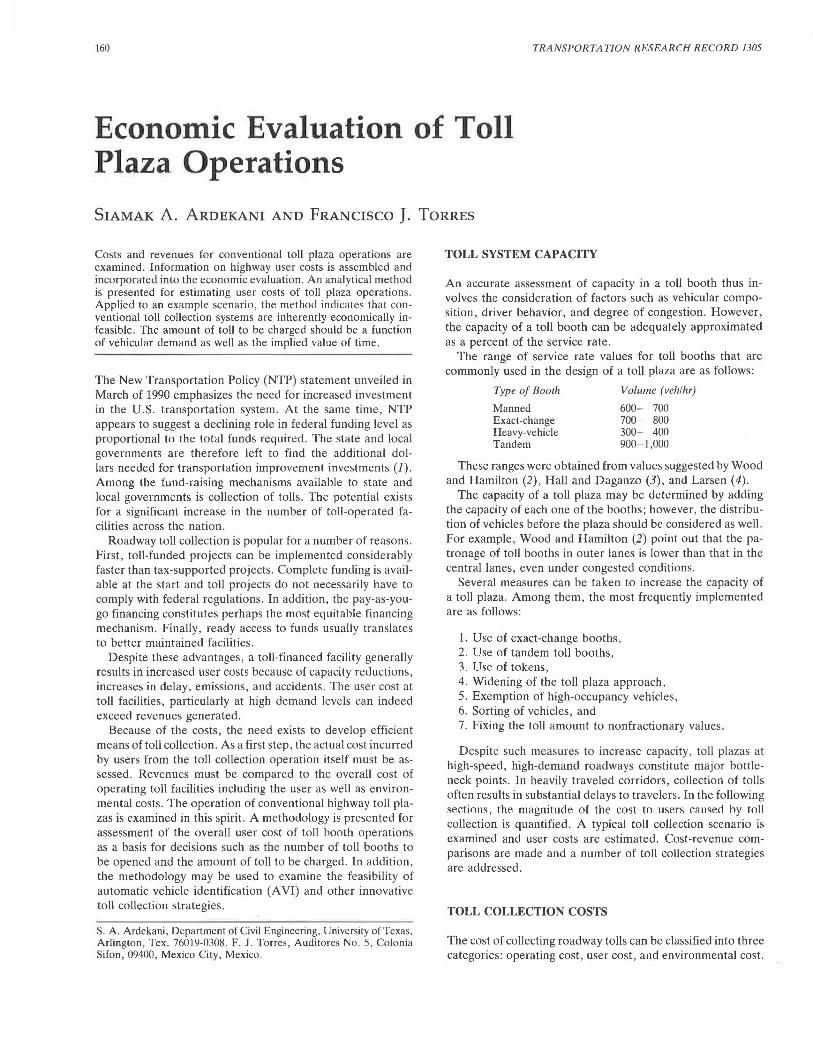
160 TRANSPORTATION RESEARCH RECORD 1305
Economic Evaluation of Toll Plaza Operations
SIAMAK A. ARDEKANI AND FRANCISCO J. TORRES
Costs and revenues for conventional toll plaza operations are examined. Information on highway user costs is assembled and incorporated into the economic evaluation. An analytical method is presented for estimating user costs of toll plaza operations. Applied to an example scenario, the method indicates that conventional toll collection systems are inherently economically infeasible. The amount of toll to be charged should be a function of vehicular demand as well as the implied value of time.
The New Transportation Policy (NTP) statement unveiled in March of 1990 emphasizes the need for increased investment in the U.S. transportation system. At the same time, NTP appears to suggest a declining role in federal funding level as proportional to the total funds required. The state and local governments are therefore left to find the additional dollars needed for transportation improvement investments (J). Among the fund-raising mechanisms available to state and local governments is collection of tolls. The potential exists for a significant increase in the number of toll-operated facilities across the nation.
Roadway toll collection is popular for a number of reasons . First, toll-funded projects can be implemented considerably faster than tax-supported projects. Complete funding is available at the start and toll projects do not necessarily have to comply with federal regulations. In addition, the pay-as-yougo financing constitutes perhaps the most equitable financing mechanism. Finally, ready access to funds usually translates to better maintained facilities.
Despite these advantages, a toll-financed facility generally results ln increased user costs because of capacity reuuclions, increases in delay, emissions, and accidents. The user cost at toll facilities, particularly at high demand levels can indeed exceed revenues generated.
Because of the costs, the need exists to develop efficient means of toll collection. As a first step. the actual cost incurred by users from the toll collection operation itself must be assessed. Revenues must be compared to the overall cost of operating toll facilities including the user as well as environmental costs. The operation of conventional highway toll plazas is examined in this spirit. A methodology is presented for assessment of the overall user cost of toll booth operations as a basis for decisions such as the number of toll booths to be opened and the amount of toll to be charged. In addition, the methodology may be used to examine the feasibility of automatic vehicle identification (A VI) and other innovative toll collection strategies.
S. A. Ardekani, Department of Civil Engineering, University of Texas. Arlington, Tex. 76019-0308. F. J . Torres, Auditores No. 5, Colonia Sifon, 09400, Mexico City, Mexico.
TOLL SYSTEM CAPACITY
An accurate assessment of capacity in a toll booth thus involves the consideration of factors such as vehicular composition, driver behavior, and degree of congestion. However, the capacity of a toll booth can be adequately approximated as a percent of the service rate.
The range of service rate values for toll booths that are commonly used in the design of a toll plaza are as follows:
Type of Booth
Manned Exact-change Heavy-vehicle Tandem
Volume (veh /hr)
600- 700 700- 800 300- 400 900-1,000
These ranges were obtained from values suggested by Wood and Hamilton (2), Hall and Daganzo (3), and Larsen (4).
The capacity of a toll plaza may be determined by adding the capacity of each one of the booths; however, the distribution of vehicles before the plaza should be considered as well. For example, Wood and Hamilton (2) point out that the patronage of toll booths in outer lanes is lower than that in the central lanes , even under congested conditions.
Several measures can be taken to increase the capacity of a toll plaza. Among them, the most frequently implemented are as follows:
1. Use of exact-change booths, 2. Use of tandem toll booths, 3. Use of tokens, 4. Widening of the toll plaza approach, 5. Exemption of high-occupancy vehicles, 6. Sorting of vehicles, and 7. Fixing the toll amount to nonfractionary values .
Despite such measures to increase capacity , toll plazas at high-speed, high-demand roadways constitute major bottleneck points. In heavily traveled corridors, collection of tolls often results in substantial delays to travelers. In the following sections, the magnitude of the cost to users c~11secl hy toll collection is quantified. A typical toll collection scenario is examined and user costs are estimated. Cost-revenue comparisons are made and a number of toll collection strategies are addressed.
TOLL COLLECTION COSTS
The cost of collecting roadway tolls can be classified into three categories: operating cost, user cost, and environmental cost.
Ardekani and Torres
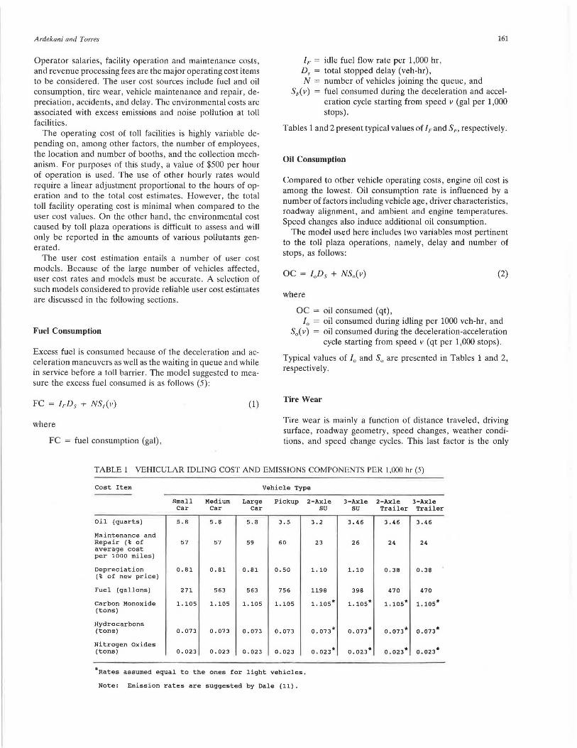
Operator salaries, facility operation and maintenance costs, and revenue processing fees are the major operating cost items to be considered. The user cost sources include fuel and oil consumption, tire wear, vehicle maintenance and repair, depreciation, accidents, and delay. The environmental costs are associated with excess emissions and noise pollution at toll facilities.
The operating cost of toll facilities is highly variable depending on, among other factors, the number of employees , the location and number of booths, and the collection mechanism. For purposes of this study, a value of $500 per hour of operation is used. The use of other hourly rates would require a linear adjustment proportional to the hours of operation and to the total cost estimates. However, the total toll facility operating cost is minimal when compared to the user cost values. On the other hand, the environmental cost caused by toll plaza operations is difficult to assess and will only be reporte.d in the amounts of various pollutants generated.
The user cost estimation entails a number of user cost models. Because of the large number of vehicles affected, user cost rates and models must be accurate . A selection of such models considered to provide reliable user cost estimates are discussed in the following sections.
Fuel Consumption
Excess fuel is consumed because of the deceleration and acceleration maneuvers as well as the waiting in queue and while in service before a toll barrier . The model suggested to measure the excess fuel consumed is as follows (5):
(1)
where
FC fuel consumption (gal),
IF = idle fuel flow rate per 1,000 hr, D, = total stopped delay (veh-hr), N = number of vehicles joining the queue , and
161
SAv) = fuel consumed during the deceleration and acceleration cycle starting from speed v (gal per 1,000 stops).
Tables 1and2 present typical values of IF and SF, respectively.
Oil Consumption
Compared to other vehicle operating costs, engine oil cost is among the lowest. Oil consumption rate is influenced by a number of factors including vehicle age, driver characteristics, roadway alignment, and ambient and engine temperatures. Speed changes also induce additional oil consumption.
The model used here includes two variables most pertinent to the toll plaza operations, namely, delay and number of stops , as follows:
where
oc
(2)
oil consumed (qt), oil consumed during idling per 1000 veh-hr, and oil consumed during the deceleration-acceleration cycle starting from speed v (qt per 1,000 stops).
Typical values of / 0 and S0 are presented in Tables 1 and 2, respectively.
Tire Wear
Tire wear is mainly a function of distance traveled, driving surface, roadway geometry , speed changes, weather conditions, and speed change cycles. This last factor is the only
TABLE 1 VEHICULAR IDLING COST AND EMISSIONS COMPONENTS PER 1,000 hr (5)
Cost Item Vehicle Type
Small Medium Large Pickup 2-Axle 3-Axle 2-Axle 3-Axle car car car SU SU Trailer Trailer
Oil (quarts) 5.8 5.8 5.8 3.5 3.2 3.46 3.46 3.46
Maintenance and Repair (% of 57 57 59 60 23 26 24 24 average cost per 1000 miles)
Depreciation 0.81 0.81 0.81 0.50 1.10 1.10 0.38 0.38 (% of new price)
Fuel (gallons) 271 563 563 756 1198 398 470 470
carbon Monoxide 1.105 1.105 1.105 1.105 i.105* i.105* i.105* 1.105* (tons)
Hydrocarbons 0.013* 0.013* o. 073* o. 073* (tons) 0.073 0.073 0.073 0.073
Nitrogen Oxides 0.023* 0.023* 0.023* 0.023* (tons) 0.023 0.023 0.023 0.023
*Rates assumed equal to the ones for light vehicles.
Note: Emission rates are suggested by Dale (11).
162 TRANSPORTATION RESEARCH RECORD 1305
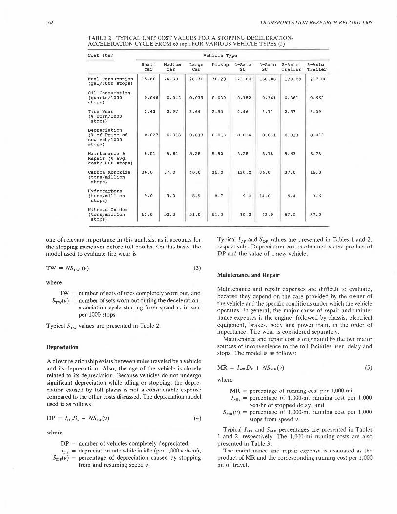
TABLE 2 TYPICAL UNIT COST VALUES FOR A STOPPING DECELERATIONACCELERATION CYCLE FROM 65 mph FOR VARIOUS VEHICLE TYPES (5)
Cost Item Vehicle Type
Small Medium Large Pickup 2-Axle 3-Axle 2-Axle 3-Axle Car Car Car SU SU Trailer Trailer
Fuel Consumption 15.60 24.30 28.30 (gal/1000 stops)
Oil consumption (quarts/1000 0.046 0.042 0.039 stops)
Tire Wear 2.43 2.97 3.64 (% worn/1000 stops)
Depreciation (% of Price of 0.027 0.018 0.013 new veh/1000 stops)
Maintenance & 5.51 5.61 5.28 Repair (% avg. cost/1000 stops)
carbon Monoxide 36.0 37.0 40.0 (tons/million stops)
Hydrocarbons (tons/million 9.0 9.0 8.9 stops)
Nitrous Oxides (tons/million 52.0 52.0 51. 0 stops)
one of relevant importance in this analysis, as it accounts for the stopping maneuver before toll booths. On this basis, the model used to evaluate tire wear is
TW = NSTw (v) (3)
where
number of sets of tires completely worn out, and number of sets worn out during the decelerationassociation cycle starting from speed v, in sets per 1000 stops
Typical S 1 w values are presented in Table 2.
Depreciation
A direct relationship exists between miles traveled by a vehicle and its depreciation. Also , the age of the vehicle is closely related to its depreciation. Because vehicles do not undergo significant depreciation while idling or stopping, the depreciation caused by toll plazas is not a considerable expense compared Lo Lhe other costs discussed. The depreciation model used is as follows:
where
(4)
number of vehicles completely depreciated, depreciation rate while in idle (per 1,000 veh-hr), percentage of depreciation caused by stopping from and resuming speed v.
30.20 123.00 168.00 179.00 217.00
0.039 0.182 0.361 0.361 0.662
2.93 4.46 3.11 2.57 3.29
o. 013 0.024 0. 031 0. 013 o. 013
5.52 5.28 5.18 5.63 6.78
35.0 130.0 36.0 37.0 15.0
8.7 9.0 14.0 5.4 3.6
51. 0 10.0 42.0 67.0 87.0
Typical / 0 p and S0 p values are presented in Tables 1 and 2, respectively. Depreciation cost is obtained as the product of DP and the value of a new vehicle.
Maintenance and Repair
Maintenance and repair expenses are difficult to evaluate, because they depend on the care provided by the owner of the vehicle and the specific conditions under which the vehicle operates. In general, the major cause of repair and maintenance expenses is the engine, followed by chassis, electrical equipment, brakes. body and power train. in the order of importance. Tire wear is considered separately.
Maintenance and repair cost is originated by the two major sources of inconvenience to the toll facilities user, delay and stops. The model is as follows:
where
(5)
percentage of running cost per 1,000 mi, percentage of 1,000-mi running cost per 1,000 veh-hr of stopped delay, and percentage of 1,000-mi running cost per 1,000 stops from speed v.
Typical /MR and SMR percentages are presented in Tables and 2, respectively . The 1,000-mi running costs are also
presented in Table 3. The maintenance and repair expense is evaluated as the
product of MR and the corresponding running cost per 1,000 mi of travel.

Ardekani and Torres 163
TABLE 3 VEHICULAR UNIT PRICES (1980 U.S. DOLLARS)
Type of Oil Maintenance vehicle (quart) and Repair
(Average cost per 1000 mi)
Small car 2.5 34.30
Medium car 2.5 41. 60
Large car 2.5 48.04
Pickup 2.5 52.81
2 Axles SU 1. 0 99.00
3 Axles SU 1. 0 140.00
2 Axles 1. 0 145.00 Trailer
3 Axles 1. 0 145.00 Trailer
•Gas Price ; 1. 221 - 0.123(tax),
**Truck tire cost includes recaps
Value of Time
Perhaps the most difficult item to evaluate among the ones considered in this analysis is the cost of the time lost by the patrons when waiting before a toll booth. There exists a basic distinction in the way the cost of time is assessed for passenger cars and for trucks. Automobile travel time savings represent nonmarket costs and they are often transformed into opportunities for additional activities, such as additional time for personal business or social activities . On the other hand, for trucks , travel time savings represent market costs.
On this basis, travel time value for a passenger car is a function of trip purpose, traveler's income level , and vehicle occupancy. The Manual on User Benefit Analysis of Highway and Bus-Transit Improvements (6) suggests a 1-hr value of (1975) U.S. $3 .90 for an average trip by a passenger car. This value was obtained from the average hourly family income prevailing in 1975 as well as the adult occupancy factor observed at that time.
For trucks, the value of time is assumed to be equivalent to the wage rate of the driver of the vehicle . According to AASHTO (6), the hourly values for single-unit and combination trucks, in 1975 dollars, are $7.00 and $8 .00, respectively.
The model which evaluates the time value is as follows:
TV = RVT(Ds + ND Ac)
where
TV= UVT (Ds +ND Ac) TV = time value,
UVT = unit value of time (dollars per hour), and D A C = delay of the acceleration-deceleration cycle .
Accident Cost
(6)
For purposes of this study, only one type of accident is considered, namely , the rear-end collision . This conflict is originated by the stopping maneuver before the toll booths.
Depreciation Fuel Tires** (New Vehicle) (gallon) (set)
6360 1. 098 43
7501 1. 098 68
9990 1. 098 75
6625 1. 098 75
8673 1. 098* 194
45350 0.886* 465
48687 0.886* 465
51630 0.886* 465
Diesel Price ; 1.01 - 0.124(tax)
A technique developed by Brown (7) to predict accidents at an intersection is used here, because the stopping maneuvers are similar at an intersection and before a toll booth.
Brown suggests the following model for an intersection:
(7)
where
AC R k =
number of accidents per million vehicles, constant that depends on the type of accident, and regression constant that accounts for variations of the vehicular flow in 1 year.
X,,Xi = two conflicting movements (veh/hr).
Brown (7) obtained a mean k value of 0.0227 with a standard deviation of0.0017 and a mean standard error of0.000555. For rear-end collisions, R = 0.7. The quantity (X;Xi)Y2 is equal to the number (N) of vehicles arriving at the toll plaza. So the number of rear-end collisions before a toll barrier can be estimated as
Ace = 0.01589 x 10- 6 N (8)
Accidents are divided into three major types according to their severity:
1. Fatal, 2. Injury (nonfatal) , and 3. Property damage.
Accident costs cited by NHTSA (8) are as follows :
Accident Type
Fatal Injury Property damage
Cost (1975 U.S. Dollars)
307,210 14,600
650
More up-to-date accident cost values have been provided by Rollins and McFarland (9).
Meyers (JO) presents accident data obtained from a survey conducted between 1976 and 1978. In this survey, data from
164
21 toll expressways were collected. Table 4 presents the percentages of occurrences computed from the values given by Rollins and McFarland (9).
The cost per accident is the summation of the products of costs and percentages of occurrences corresponding to three types of accident, as follows:
where
Cacc = cost per accident ($), Cr •• = cost of a fatal accident ($), Pr.1 = occurrence percentage of a fatal accident, cinj = cost of an injury accident, P ini = occurrence percentage of an injury accident, Cpd = cost of a property damage accident, and Ppd = occurrence percentage of a property damage
accident.
(9)
The unit cost obtained in Equation 9 is multiplied by the number of accidents computed using Equation 8 to estimate the total accident cost.
TOXIC EMISSIONS MODELS
Vehicular emissions constitute a major source of environmental pollution. In this work, models to evaluate carbon monoxide, hydrocarbons, and oxides of nitrogen are presented. However, no attempt is made to estimate the cost of the environmental deterioration caused by these vehicular emissions. Carbon monoxide and hydrocarbon emissions result from incomplete combustion of fuel during the operation of internal combustion engines. Oxides of nitrogen are produced when the oxygen and nitrogen in the air used by internal combustion engines combine umler Lht: ht:al and pressure of the combustion process.
The emission model for carbon monoxide is
ECO = lcoDs + NSco(v) (10)
where
ECO = total carbon monoxide emitted (lb), fco = carbon monoxide emission per 1,000 veh-hr (lb),
and Sc0 (v) = carbon monoxide emitted per 1,000 stops from
speed v (lb) .
Hydrocarbons emitted are evaluated according to the following model:
(11)
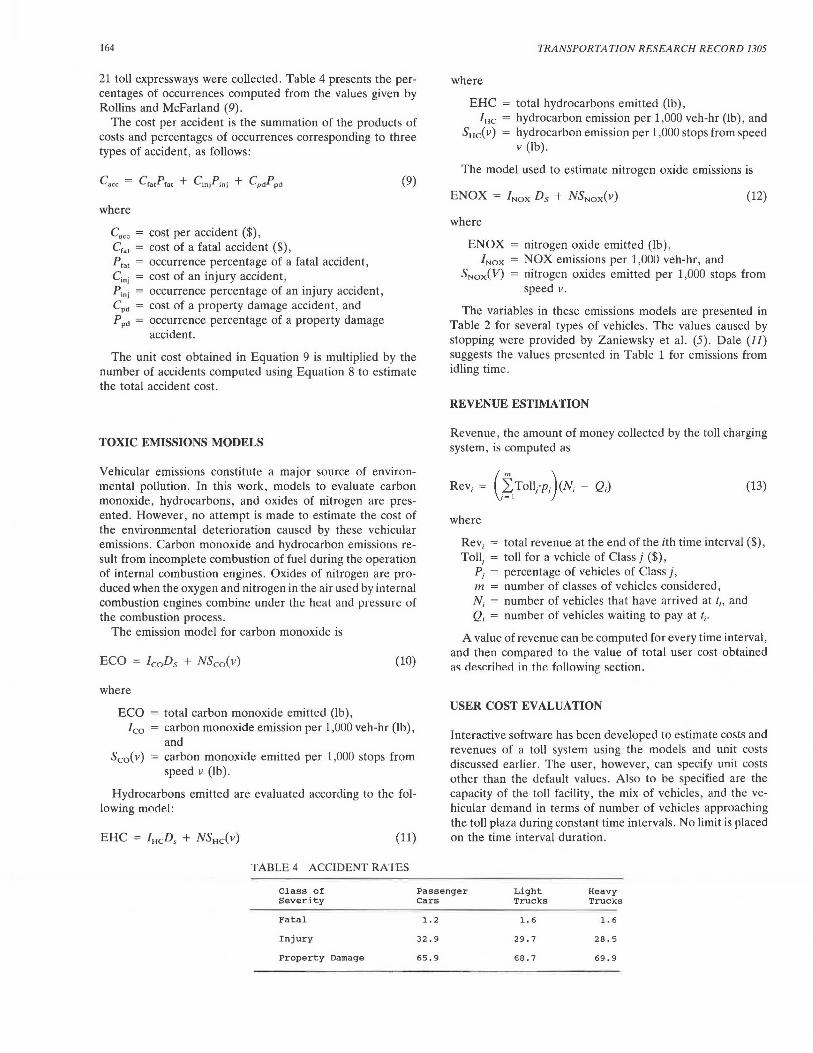
TABLE 4 ACCIDENT RATES
TRANSPORTATION RESEARCH RECORD 1305
where
EHC = total hydrocarbons emitted (lb), /He = hydrocarbon emission per 1,000 veh-hr (lb), and
SHc(v) = hydrocarbon emission per 1,000 stops from speed v (lb).
The model used to estimate nitrogen oxide emissions is
ENOX = /Nox D5 + NSNox(v) (12)
where
ENOX = nitrogen oxide emitted (lb), /Nox = NOX emissions per 1,000 veh-hr, and
SNox(V) = nitrogen oxides emitted per 1,000 stops from speed v.
The variables in these emissions models are presented in Table 2 for several types of vehicles. The values caused by stopping were provided by Zaniewsky et al. (5). Dale (1/) suggests the values presented in Table 1 for emissions from idling time.
REVENUE ESTIMATION
Revenue, the amount of money collected by the toll charging system, is computed as
(13)
where
Rev; = total revenue at the end of the ith time interval($) , Tolli = toll for a vehicle of Class j ($),
Pi = percentage of vehicles of Class j, m number of classes of vehicles considered, N,. = number of vehicles that have arrived at t1, and Q; = number of vehicles waiting to pay at t; .
A value of revenue can be computed for every time interval, and then compared to the value of total user cost obtained <lS rlesr.riherl in the following section.
USER COST EVALUATION
Interactive software has been developed to estimate costs and revenues of a toll system using the models and unit costs discussed earlier. The user, however, can specify unit costs other than the default values. Also to be specified are the capacity of the toll facility, the mix of vehicles, and the vehicular demand in terms of number of vehicles approaching the toll plaza during constant time intervals. No limit is placed on the time interval duration.
Class of Passenger Light Heavy severity Cars Trucks Trucks
Fatal 1. 2 1. 6 1. 6
Injury 32.9 29.7 28.5
Property Damage 65.9 68.7 69.9
Ardekani and Torres
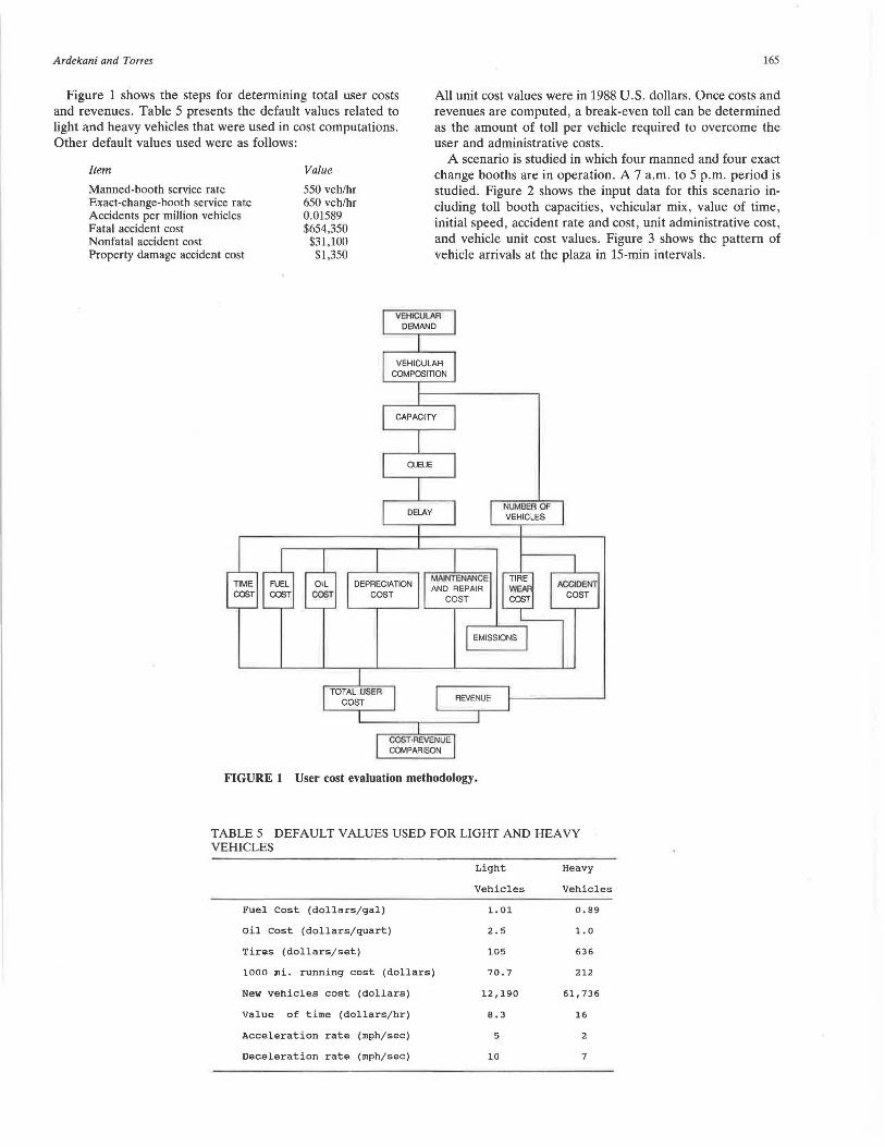
Figure 1 shows the steps for determining total user costs and revenues. Table 5 presents the default values related to light and heavy vehicles that were used in cost computations. Other default values used were as follows:
Item
Manned-booth service rate Exact-change-booth service rate Accidents per million vehicles Fatal accident cost Nonfatal accident cost Property damage accident cost
Value
550 veh/hr 650 veh/hr 0.01589 $654,350 $31,100 $1,350
165
All unit cost values were in 1988 U.S. dollars. Once costs and revenues are computed, a break-even toll can be determined as the amount of toll per vehicle required to overcome the user and administrative costs.
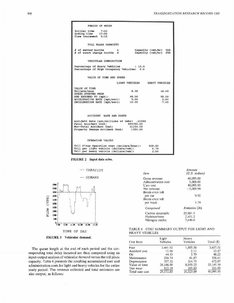
A scenario is studied in which four manned and four exact change booths are in operation. A 7 a.m. to 5 p.m. period is studied. Figure 2 shows the input data for this scenario including toll booth capacities, vehicular mix, value of time, initial speed, accident rate and cost, unit administrative cost, and vehicle unit cost values. Figure 3 shows the pattern of vehicle arrivals at the plaza in 15-min intervals.
VEHICULAR DEMAND
TOTAL USER COST
MAlNTENANCE AND REPAIR
COST
COST-REVENUE COMPARISON
REVENUE
FIGURE 1 User cost evaluation methodology.
NUl~Bffi OF VEHICLES
ACCIDENT COST
TABLE 5 DEFAULT VALUES USED FOR LIGHT AND HEAVY VEHICLES
Fuel Cost (dollars/gal)
Oil Cost (dollars/quart)
Tires (dollars/set)
1000 mi. running cost (dollars)
New vehicles cost (dollars)
Value of time (dollars/hr)
Acceleration rate (mph/sec)
Deceleration rate (mph/sec)
Light
Vehicles
1. 01
2.5
105
70.7
12,190
8.3
5
10
Heavy
Vehicles
0.89
1. 0
636
212
61,736
16
2
7
166 TRANSPORTATION RESEARCH RECORD 1305
&8811 "
me 4RAll
me :i:: me p.. :> me
3: me
0 18BB ...:i
1291 r.. &119
I 1.88
PERIOD OF STUDY
Initial time Ending time Time increment
7:00 17:00
0:15
TOLL PLAZA CAPACITY
# of manned booths 4 # of exact change booths 4
VEHICULAR COMPOSITION
Capacity (veh/hr) 550 Capacity (veh/hr) 650
Percentage of Heavy Vehicles : 15.0 Percentage of High Occupancy Vehicles: o.o
VALUE OF TIME AND SPEED
LIGHT VEHICLES
VALUE OF TIME Dollars/hour SPEED STOPPED FROM AND RESUMED TO (mph): ACCELERATION RATE (mph/sec): DECELERATION RATE (mph/sec):
ACCIDENT RATE AND COSTS
8.30
65.00 5.00
10.00
HEAVY VEHICLES
16.00
55.00 2.00 7.00
Accident Rate (ace/millions of Fatal Accident Cost: Non-Fatal Accident Cost: Property Damage Accident Cost:
vehs) • 01589 654350.00
31100. 00 1350.00
OPERATION VALUES
Toll Plaza Operation cost (dollars/hour): Toll per light vehicle (dollars/veh): Toll per heavy vehicle (dollars/veh):
FIGURE 2 Input data echo.
CAPACITY
DEMAND
!.89 11 .llll ' ll .BB IS.BB !?.
500.00 0.75 2.00
Item
Gross revenue Administration cost User cost Net revenue Break-even toll per car
Break-even toll per truck
Compound
Carbon monoxide Hydrocarbons Nitrogen oxides
Amount (U.S. dollars)
40,095.00 5,000.00
40,095.95 -5,000.94
0.92
1.74
Emission (lb)
25,981.5 2,451.2 7,640.0
TIME OF DAY TABLE 6 COST SUMMARY OUTPUT FOR LIGHT AND
FIGURE 3 Vehicular demand.
The queue length at the end of each period and the corresponding total delay incurred are then computed using an input-output analysis of vehicular demand versus the toll plaza capacity. Table 6 presents the resulting accumulated user and administration costs for light and heavy vehicles for the entire study period. The revenue collected and total emissions are also output, as follows:
HEAVY VEHICLES
Cost Item
Fuel Accident cost Oil Maintenance Depreciation Value of time Tire wear Total user cost
Light Vehicles
2,601.92 11.06 44.53
256.74 357.32
26,186.09 115.19
29,572.85
Heavy Vehicles Total($)
1,055.58 3,657.51 2.11 13.17 3.70 48.22
81.87 338.61 314.75 672.07
8,959.25 35,145.34 105.83 221.02
10,523.09 40,095.95
Ardekani and Torres
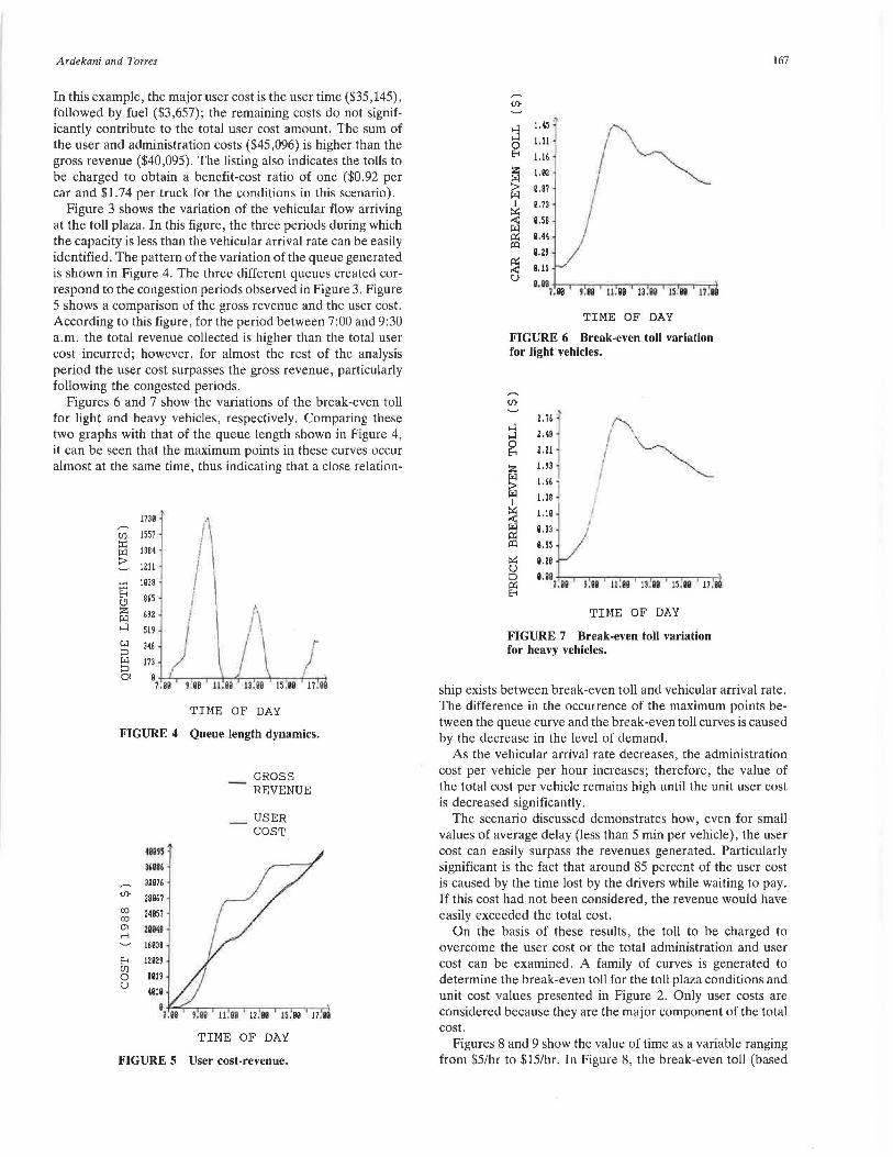
In this example, the major user cost is the user time ($35,145), followed by fuel ($3,657); the remaining costs do not significantly contribute to the total user cost amount. The sum of the user and administration costs ($45,096) is higher than the gross revenue ($40,095). The listing also indicates the tolls to be charged to obtain a benefit-cost ratio of one ($0.92 per car and $1. 74 per truck for the conditions in this scenario).
Figure 3 shows the variation of the vehicular flow arriving at the toll plaza. In this figure, the three periods during which the capacity is less than the vehicular arrival rate can be easily identified. The pattern of the variation of the queue generated is shown in Figure 4. The three different queues created correspond to the congestion periods observed in Figure 3. Figure 5 shows a comparison of the gross revenue and the user cost. According to this figure, for the period between 7:00 and 9:30 a.m. the total revenue collected is higher than the total user cost incurred; however, for almost the rest of the analysis period the user cost surpasses the gross revenue, particularly following the congested periods.
Figures 6 and 7 show the variations of the break-even toll for light and heavy vehicles, respectively. Comparing these two graphs with that of the queue length shown in Figure 4, it can be seen that the maximum points in these curves occur almost at the same time, thus indicating that a close relation-
17311
en 1557
~ 1384
> 1211
::r:: 1038 8 L'J z fl:< ,_:i
865
692
519
~ 346
~ 173
/\ I
I
0 \et u0 11.ee 1u0 15.'00 17.Q
TIME OF DAY
FIGURE 4 Queue length dynamics.
<Jr
co co m r-1
8 en 0 u
499!~
3'986
32076
281167
24057
211948
16038
12029
8019
4010
GROSS REVENUE
USER COST
8-t-<r-...-...-...-...-~-.---.--.--,-J 1.80 ua II .Be JUG 15. 011 17 .
TIME OF DAY
FIGURE 5 User cost-revenue.
<Jr
,_:i J.45 .
I~ ,_:i J.31 0 8 J.16 :z; J.92 fl:< > 11.87 fl:< I 0. 73
::..:: < 11.58 fl:< 0:: 11.44 co
B.29
~ B.15 u
Ull 1.1111 !.1111 11 .011 13 .88 Jl .118 H ,
TIME OF DAY
FIGURE 6 Break-even toll variation for light vehicles.
<Jr
,_:i ,_:i 0 8
:z; fl:< > fl:< I
::..:: < fl:< 0:: co ~ u ;:J 0:: 8
2.76 '
2.48
2.21
J. 93
J. 66
1.38 -
J.10
B.83
e.55
B.28
ua 1.ea
' I i
i.ea 11 .96 13 .ee is .Bi 11 .
TIME OF DAY
FIGURE 7 Break-even toll variation for heavy vehicles.
167
ship exists between break-even toll and vehicular arrival rate. The difference in the occurrence of the maximum points between the queue curve and the break-even toll curves is caused by the decrease in the level of demand.
As the vehicular arrival rate decreases, the administration cost per vehicle per hour increases; therefore, the value of the total cost per vehicle remains high until the unit user cost is decreased significantly.
The scenario discussed demonstrates how, even for small values of average delay (less than 5 min per vehicle), the user cost can easily surpass the revenues generated. Particularly significant is the fact that around 85 percent of the user cost is caused by the time lost by the drivers while waiting to pay. If this cost had not been considered, the revenue would have easily exceeded the total cost.
On the basis of these results, the toll to be charged to overcome the user cost or the total administration and user cost can be examined. A family of curves is generated to determine the break-even toll for the toll plaza conditions and unit cost values presented in Figure 2. Only user costs are considered because they are the major component of the total cost.
Figures 8 and 9 show the value of time as a variable ranging from $5/hr to $15/hr. In Figure 8, the break-even toll (based

168
Toi I needed to overco Me user cos t <cars)
1.jQ 1 7.11
6.32 1 5.53 -
TUU! \'AUl t. 1 9"
4. 74
3.95
3.16
2.37
1.58
Q, 79
a.ea UQ a.ze
FIGURE 8 Toll to be charged as a function of waiting time in queue.
s.99
ts9
4.99
3,59
3.00
2.59
2.09
1.s9
1.99
8.58
Joli needed to ovtl'COMt user cost (urs>
Onehourperiocl.
deMand/capaeity
FIGURE 9 Toll to be charged as a function of the demand-capacity ratio for some values of times.
on user cost) plotted as a function of the average delay per vehicle indicates a linear relation between the two variables . On the other hand, Figure 9 shows the break-even toll versus the demand-capacity ratio. Both figures suggest that to compensate for user costs, higher tolls should be charged at higher demand levels. However, as shown in Figure 9, the toll values are asymptotic at high demand-capacity values. For example , at a $5/hr value of time, the asymptotic toll amount is about $1.50 per car, versus about $3.50 per car for a $10/hr value of time. These values assume that the demand-capacity values specified persist for a 1-hr period.
SUMMARY AND DISCUSSION
An attempt has been made to assess the cost incurred by drivers when using a toll facility . A major concern has been to provide estimation models for all the possible cost generators, even if, as observed for some items, the contribution to the total user cost is relatively small.
For the economic analysis described, variables such as degree of congestion and vehicular composition should be taken into account in the evaluation of the toll plaza capacity. Including these variables would constitute research in itse lf, because the literature on toll facility operations is not extensive . If a criterion to assess a unit cost for toxic emissions is eventually set, the effectiveness of the procedure described could also be significantly enhanced.
A major contribution of this work has been the collection and synthesis of a large amount of scattered information on highway user costs and their incorporation into the economic analysis of toll plaza operations. The procedure described can be easily applied to determine the cost-effectiveness of the charging process in a toll plaza. Furthermore, its use could
TRANSPORTATION RESEARCH RECORD 1305
be expanded to a whole set of toll collection points, allowing the evaluation of a complete collection system.
The break-even toll has been defined as the toll to be charged to compensate for the toll collection cost. The user cost has been used in this study as the basis for calculating the breakeven toll because it constitutes a major portion (up to 90 percent) of the total toll collection cost. The break-even toll may be considered in setting the toll value for a facility. For example, the toll authority may define a total toll cost as the sum of the toll to be charged and the break-even toll. The policy may then be to set the toll value such that the so-defined total toll cost will not exceed the excess travel cost on alternative routes. From this viewpoint, tolls could only be increased if the facility operator took actions to reduce user and other costs or if the travel cost on alternative routes increased.
This methudulugy is also useful in assessing lhe economic feasibility of an A VI method and in setting demand-related variable toll charges for A VI systems. A study carried out by the Hong Kong governmenJ (12) indicated that there are no major technological barriers for the implementation of an A VI system; however, its introduction depends on political considerations (13) as well as the economical advantages it could offer compared with traditional charging systems. One such economic advantage is the reduction or elimination of the user costs evaluated in this research.
RF.FF.RF.NCF.S
1. R. F. Beaubien. Can Technology Save Us? Institute of Transportation Engineers Journal, June 1990.
2. H. C. Wood and C. S. Hamilton. Design of Toll Plazas from the Operator's Viewpoint. HRB Proc., Vol. 34, 1955.
3. R. Hall and C. Daganzo . Tandem Toll Booths for the Golden Gate Bridge. In Transportation Research Record 910, TRB, National Research Council, Washington , D.C., 1983.
4. 0. Larsen. Toll Ring in Bergen , Norway. In Transportation Research Record 1107, TRB , National Research Council , Washington, D.C., 1987.
5. J. B. Zanicwsky, B. C . Butler, G. Cunningham, G. E. Elkins, M. S. Paggi, and R. Machemehl. Vehicle Operating Costs, Fuel Consumption, and Pavement Type and Conditions Factors. FHWA, U.S. Department of Transportation, March 1982.
6. A Manual on User Benefit Analysis of Highway and Bus Transit Improvements. AASHTO, Washington, D.C., 1977.
7. R. Brown. A Method for Determining the Accident Potential of an Intersection . Traffic Engineering and Control, Dec. 1981, pp. 684-651.
8. Societal Costs of Motor Vehicle Accidents. Preliminary Report, NHTSA, U.S . Department of Transportation, April 1975.
9. J. B. Rollins and W. F . McFarland . Cost of Motor Vehicle Accidents and Injuries. In Transportation Research Record 1068, TRB, National Research Council, Washington , D.C. , 1986.
10. W. S. Meyers. Comparison of Truck and Passenger-Car AcCident Rates on Limited-Access Facilities. In Transportation Research Record 808, TRB, National Research Council, Washington, D.C., 1981.
11. C. S. Dale. Procedure for Estimating Highway User Costs, Fuel Consumption and Air Pollution. Office of Traffic Operations, FHWA, U.S. Department of Transportation, May 1980.
12. I. Catling and G. Roth . Electronic Road Pricing in Hong Kong : An Opportunity for Road Privatization? In Transportation Research Record 1107, TRB, National Research Council, Washington, D .C., 1987.
13. S. F. Borns . The Political Economy of Road Pricing: The Case of Hong Kong. Proc., World Conference on Transportation Research, May 1986.
Publication of this paper sponsored by Committee on Transportation Economics.