Embed Size (px)
Citation preview

David Tenenbaum – GEOG 110 – UNC-CH Fall 2005
Ecosystem Modeling with STELLA• Throughout this course, we have focused upon models
that deal with the change of some phenomenon in an ecosystem in time
• STELLA and its associated systems view is very well suited to this purpose: – By representing the particular quantity of interest using a
stock, and then applying flows (and the converters and connectors that control them) to that stock by a solving a difference equation, STELLA can calculate the state of that stock at any number of time steps into the future
• This is a very useful and complete framework if we want to consider the state of a particular object or part of an ecosystem in isolation (i.e. the DO in a river reach just below a treatment plant)

David Tenenbaum – GEOG 110 – UNC-CH Fall 2005
Components of a Model
Mathematical models have three basic components: The input data, the algorithmic portion that does the modeling, and outputs that describe the results
Nix, S.J. 1994. Urban Stormwater Modeling and Simulation. Lewis Publishers, U.S.A., p. 23.

David Tenenbaum – GEOG 110 – UNC-CH Fall 2005
Spatial Ecosystem Modeling with GIS• However, the discipline of Geography is equally
interested (or perhaps more interested) in the change of phenomena (in ecosystems or other contexts) in space
• Thus, the STELLA-style approach we have used so far in this course ignores some key aspects of describing ecosystems which are popular with geographers:– Phenomena work differently in different locations– We can better understand those phenomena and the
underlying processes that make them function by describing them in terms of their distribution in space (mapping)
– We can subdivide ecosystems into smaller units and study each in isolation to figure out how things are working
– We can model the interactions between the smaller units

David Tenenbaum – GEOG 110 – UNC-CH Fall 2005
Lumped vs. Distributed Models• We can distinguish between two types of models:• Lumped Models – These are the sorts of STELLA
models we have used so far in this course– They represent inputs and responses in terms of the
dimensions of time and whatever is being modeled(issues of location and associated dimensions of length, area and volume are often absent)
– No account is taken of variation within the entity being modeled: It is assumed to be homogenous and well-mixed, i.e. Suppose we were running the model from Lab 5 for a particular forest stand. Even though there are likely various types of trees, canopy heights and densities, variations in soil etc. we model that forest stand using a single LAI and K, and with uniform soil characteristics etc.

David Tenenbaum – GEOG 110 – UNC-CH Fall 2005
Lumped vs. Distributed Models• Distributed Models – These sorts of models take the
variation of phenomena in space into account in their model structure– Both inputs and responses have a spatial aspect to them,
i.e. mapped information is required as part of the input, and the output includes spatial pattern information
– Distributed models are thus very useful when it comes to representing and studying variation. While the modeled sub-units still usually use the assumptions of homogeneity and being well-mixed, the units’ size and shape are adjusted to make these assumptions as reasonable as possible, i.e. Perhaps the forest stand we are modeling consists of 2 or 3 distinctly different sub-units, each with distinct species, and canopy and soil characteristics. We could then model each of these sub-units with its own parameters.
David Tenenbaum – GEOG 110 – UNC-CH Fall 2005
Ecosystem Representation in Distributed Models
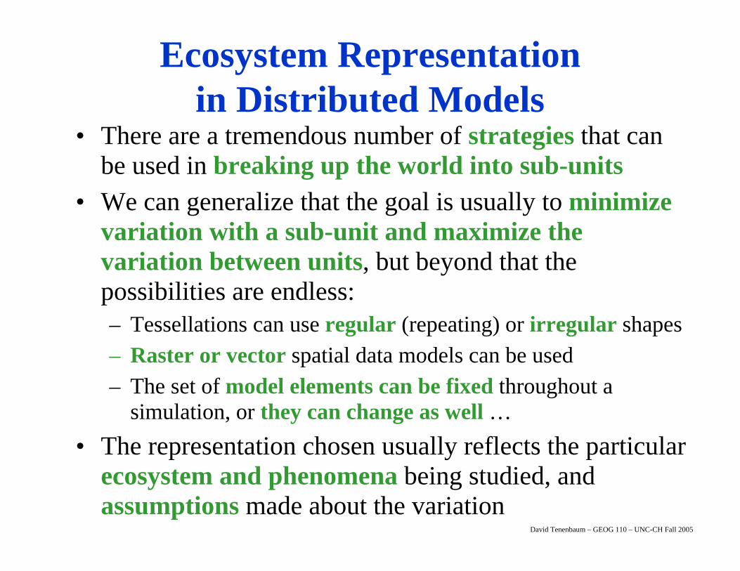
• There are a tremendous number of strategies that can be used in breaking up the world into sub-units
• We can generalize that the goal is usually to minimize variation with a sub-unit and maximize the variation between units, but beyond that the possibilities are endless:– Tessellations can use regular (repeating) or irregular shapes– Raster or vector spatial data models can be used– The set of model elements can be fixed throughout a
simulation, or they can change as well …• The representation chosen usually reflects the particular
ecosystem and phenomena being studied, and assumptions made about the variation

David Tenenbaum – GEOG 110 – UNC-CH Fall 2005
Representing the Real World w/ Models
• The figure to the left depicts a hierarchy for (spatial) models of knowledge about the real world
• This set of spatial modelsincludes a few sorts of spatial representations that can be used in conjunction with RHESSys
• In the case of our STELLA models, issues of location and spatial arrangement have been unimportant, so it was possible to skip directly from the Real World to a semantic model
Maidment, D.R. 1993. GIS and Hydrologic Modeling. In Goodchild, M.F., B.O. Parks, and L.T. Steyeart (Eds.). Environmental Modeling and GIS, Oxford University Press, New York, p. 157.

David Tenenbaum – GEOG 110 – UNC-CH Fall 2005
Regional HydroEcological Simulation System (RHESSys)
• The Regional HydroEcological Simulation System (RHESSys) is a GIS-based hydroecological modeling framework designed to simulate water, carbon, and nutrient fluxes
• By combining a set of physically-based process models and a methodology for partitioning and parameterizing the landscape, RHESSys is capable of modeling the spatial distribution and spatio-temporal interactions between different processes at the watershed scale

David Tenenbaum – GEOG 110 – UNC-CH Fall 2005
How Does RHESSys Represent the Landscape?
• It models processes at spatial and temporal scaleswhich efficiently and effectively represent landscapeheterogeneity:– Temporal - Through time step iterations of processes in
the model execution (some processes are computed daily, while others are computed hourly since the hourly variation makes a difference, and reaggregated to a daily time step)
– Spatial - Through a landscape representation that enforces hierarchically contained object partitions, meaning that the entire watershed’s extent is broken up into a set of basins, each basin is broken up into a set of zones, etc.
• Different processes are simulated using objects at different levels in the hierarchy

David Tenenbaum – GEOG 110 – UNC-CH Fall 2005
Regional HydroEcological Simulation System (RHESSys)

David Tenenbaum – GEOG 110 – UNC-CH Fall 2005
RHESSys Process Based Sub-Models•Conceptually, the way RHESSys does its calculations is like any STELLA model, simply applied in a more complex fashion:•State variables keep track of the quantity of matter/energy of a particular sort in a particular object (just like Stocks do)
•Matter and energy can move between particular stores within an object OR can move between objects (this is a key difference) according to the process models (much like Flows) as applied at the appropriate level of the object hierarchy:
•Meteorological processes use the MT-CLIM model operating in Zones•Hydrologic processes use either TOPMODEL or DHSVM in Hillslopesand Patches•Canopy processes use BIOME-BGC running at the Stratum level

David Tenenbaum – GEOG 110 – UNC-CH Fall 2005
RHESSys Object Hierarchy

David Tenenbaum – GEOG 110 – UNC-CH Fall 2005
RHESSys Inputs• RHESSys makes use of a few kinds
of input data (other than the spatial description) to set up a model run:
• Values are drawn from a library of vegetation, soil, and land-use parameters to describe those characteristics of the landscape that will not change through the model run. These are called default parameters, and their role is similar to that of Converters in STELLA
• Also required is time series information, such as daily temperature and precipitation information (in STELLA we might use a Graphical Converter for this)
• One time events (disturbances) can also be included

David Tenenbaum – GEOG 110 – UNC-CH Fall 2005
Landscape Representation through Object Partitioning
• RHESSys divides the landscape into a series of successively contained partitions:
1) The method for creating a partition is determined by the processes it will represent
2)
Once landscape objects in a partition are defined, parameters at that level are determined
3)

David Tenenbaum – GEOG 110 – UNC-CH Fall 2005
RHESSys GIS Preprocessing
DEM VEG
STR SOIL
David Tenenbaum – GEOG 110 – UNC-CH Fall 2005
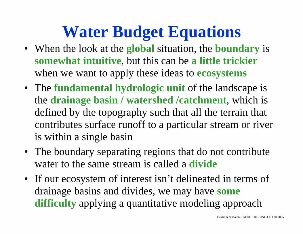
Water Budget Equations• When the look at the global situation, the boundary is
somewhat intuitive, but this can be a little trickierwhen we want to apply these ideas to ecosystems
• The fundamental hydrologic unit of the landscape is the drainage basin / watershed /catchment, which is defined by the topography such that all the terrain that contributes surface runoff to a particular stream or river is within a single basin
• The boundary separating regions that do not contribute water to the same stream is called a divide
• If our ecosystem of interest isn’t delineated in terms of drainage basins and divides, we may have some difficulty applying a quantitative modeling approach

David Tenenbaum – GEOG 110 – UNC-CH Fall 2005
Water Budget Equations• This leaves us with the following equation:
dVdt = 0 = p - so - et p = so + etor
Hornberger et al. 1998. Elements of Physical Hydrology. The Johns Hopkins University Press, Baltimore and London.
David Tenenbaum – GEOG 110 – UNC-CH Fall 2005
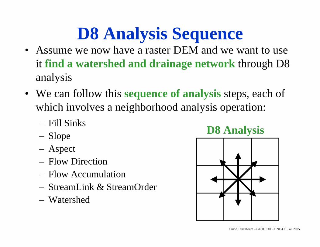
• Assume we now have a raster DEM and we want to use it find a watershed and drainage network through D8 analysis
• We can follow this sequence of analysis steps, each of which involves a neighborhood analysis operation:– Fill Sinks– Slope– Aspect– Flow Direction– Flow Accumulation– StreamLink & StreamOrder– Watershed
D8 Analysis Sequence
D8 Analysis

David Tenenbaum – GEOG 110 – UNC-CH Fall 2005
Fill Sinks•We need a DEM that does not have any depressions or pits in it for D8 drainage network analysis
•The first step is to remove all pits from our DEM using a pit-filling algorithm
•This illustrationshows a DEM of Morgan Creek, west of Chapel Hill

David Tenenbaum – GEOG 110 – UNC-CH Fall 2005
Flow Direction and Accumulation•Slope and aspect are needed to produce flow direction, which assigns each cell a direction of steepestdescent•Flow accumulationuses flow direction to find the number of cells that drain toeach cell•Taking the log of accumulation makes the pattern much easier to see

David Tenenbaum – GEOG 110 – UNC-CH Fall 2005
Stream Links, Order, and Basins•By selecting a threshold value for flow accumulation, we can produce a stream network
•This network can divided into stream links, which can in turn be assigned stream order values using network analysis methods
•Threshold=1 gives the watershed

David Tenenbaum – GEOG 110 – UNC-CH Fall 2005
RHESSys GIS Preprocessing
DEM STR
DigitalTerrain
Analysis
WORLD HILLSLOPES
David Tenenbaum – GEOG 110 – UNC-CH Fall 2005
Topographic Moisture Index
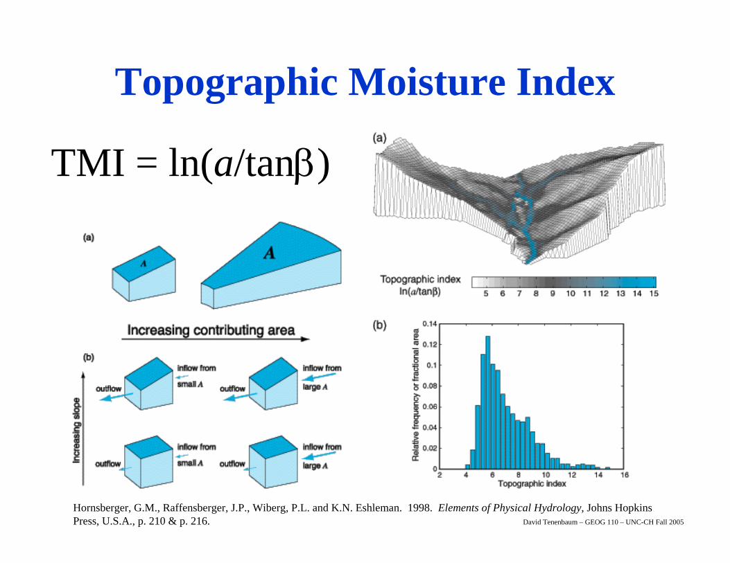
TMI = ln(a/tanβ)
Hornsberger, G.M., Raffensberger, J.P., Wiberg, P.L. and K.N. Eshleman. 1998. Elements of Physical Hydrology, Johns Hopkins Press, U.S.A., p. 210 & p. 216.

David Tenenbaum – GEOG 110 – UNC-CH Fall 2005
RHESSys GIS Preprocessing
VEG
SOIL
WETNESS INDEX
PATCHES
OverlayAnalysis

David Tenenbaum – GEOG 110 – UNC-CH Fall 2005
RHESSys GIS Preprocessing

David Tenenbaum – GEOG 110 – UNC-CH Fall 2005
RHESSys Output• Like STELLA, RHESSys can be used to
track the changes in a state variable over time, in that the model produces a series of values for each timestep of the model run
• Key differences here are that RHESSys produces hundreds of different output values (various quantities related to water, carbon and nutrients) that can be consumed in this way for EACH object!
• Alternatively, the same value for each object from the same timestep can be mapped, to produce spatial outputs that show the pattern of values