Erik Parner, Department of Biostatistics, Aarhus University©

Erik Parner Basic Biostatistics - Day 8 1

PhD course in Basic Biostatistics – Day 8Erik Parner, Department of Biostatistics, Aarhus University©

Time-to-event dataSurvival with malignant melanoma

The survival function and the cumulative mortality proportion The Kaplan-Meier estimateRight censored dataWarnings concerning the Kaplan-Meier estimate: Interval censored data and Competing risk

Comparing survival in two groupsThe log-rank test

The hazard function

The simple Cox-proportional hazard modelThe model, estimation, validation

The general Cox- model


Overview

Data to analyse Type of analysis Unpaired/Paired Type Day

Continuous One sample mean Irrelevant Parametric Day 1

Nonparametric Day 3

Two sample mean Non-paired Parametric Day 2

Nonparametric Day 2

Paired Parametric Day 3

Nonparametric Day 3

Regression Non-paired Parametric Day 5

Several means Non-paired Parametric Day 6

Nonparametric Day 6

Binary One sample mean Irrelevant Parametric Day 4

Two sample mean Non-paired Parametric Day 4

Paired Parametric Day 4

Regression Non-paired Parametric Day 7

Time to event One sample: Cumulative risk Irrelevant Nonparametric Day 8

Regression: Rate/hazard ratio Non-paired Semi-parametric Day 8


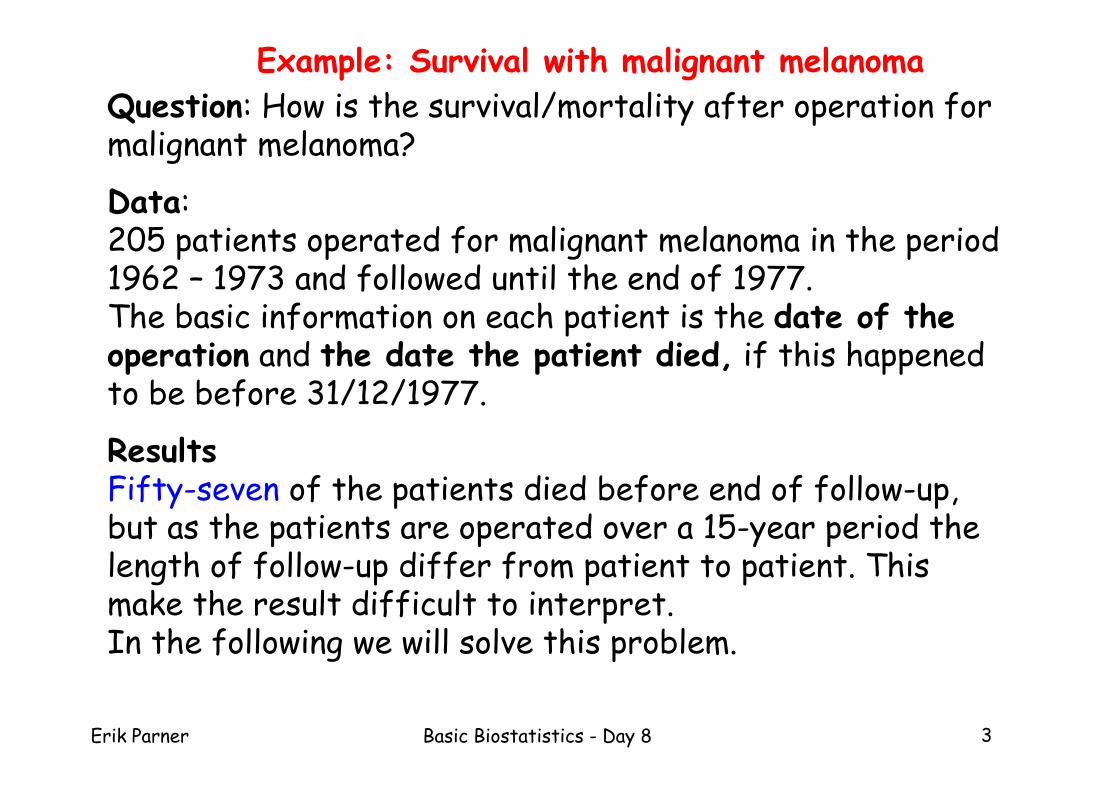
Example: Survival with malignant melanoma

Question: How is the survival/mortality after operation for malignant melanoma?

Data: 205 patients operated for malignant melanoma in the period 1962 – 1973 and followed until the end of 1977. The basic information on each patient is the date of the operation and the date the patient died, if this happened to be before 31/12/1977.

ResultsFifty-seven of the patients died before end of follow-up, but as the patients are operated over a 15-year period the length of follow-up differ from patient to patient. This make the result difficult to interpret.In the following we will solve this problem.


Survival analysis with equal follow-up time

Consider data on survival among patients with tuberculosis treated with either Streptomycin or placebo (day 4).

Everybody was followed for 6 months, and so it was possible to estimate risk of dying as

number of deaths before 6 months

number alive at time zero

Everybody dying later than six months were in effect right-censored after six months.

But before six months of follow-up there was no censoring, only death terminated follow-up.


0

50

100

150

200id

01/01/62 01/01/70 01/01/74 01/01/78calendar time

deaddate of operation/end of follow up

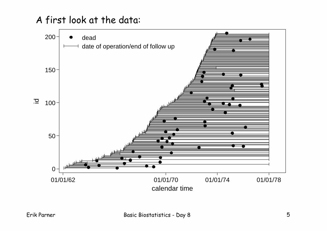
A first look at the data:


The plot on the previous slide uses calendar time as the time scale.

This could be a relevant time scale for many studies.

Other choices of time scales can be:

•Age

•Time since diagnosis

•Time since first symptoms

Here the relevant time scale is time since operation.

The choice of time scale is the first and most essential choice in all studies involving time-to-event data.

Time scales


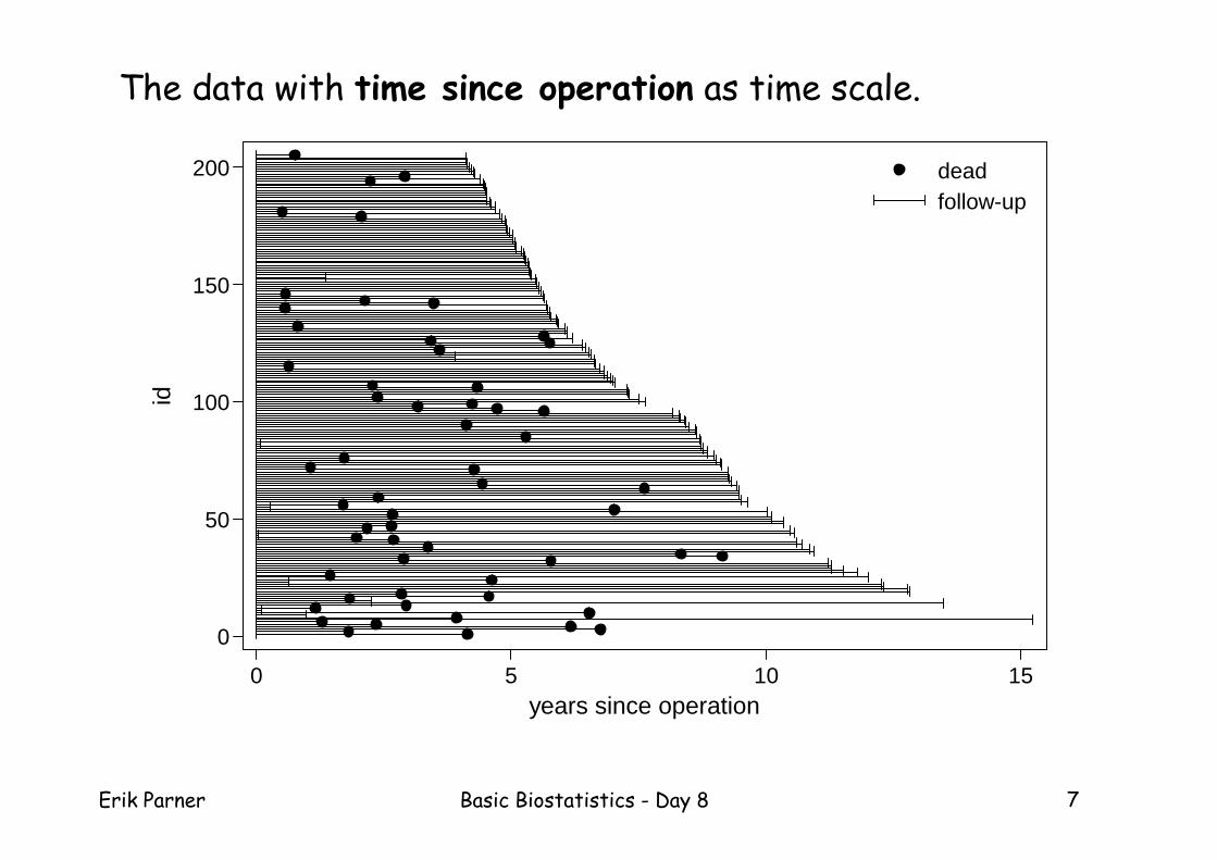
The data with time since operation as time scale.

0

50

100

150

200id

0 5 10 15years since operation

deadfollow-up


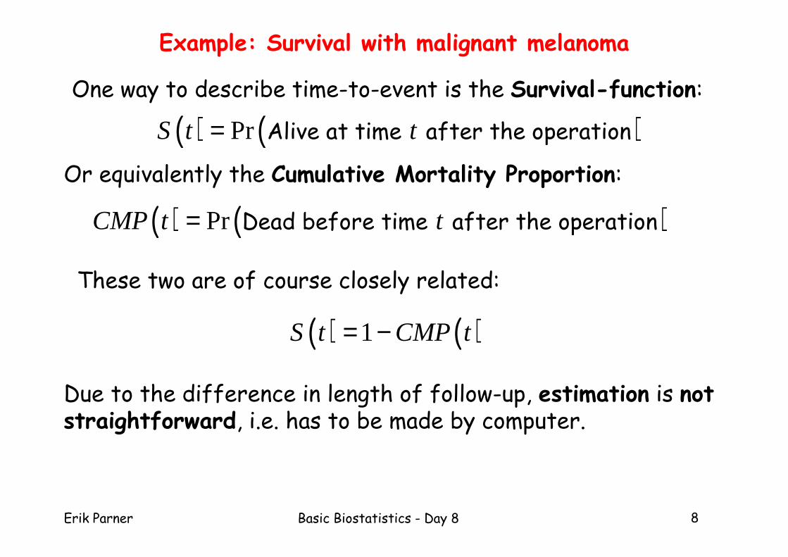
One way to describe time-to-event is the Survival-function:

( ) ( )Pr Alive at time after the operation S t t=

Or equivalently the Cumulative Mortality Proportion:

( ) ( )Pr Dead before time after the operation CMP t t=

These two are of course closely related:

( ) ( )1S t CMP t= −

Example: Survival with malignant melanoma

Due to the difference in length of follow-up, estimation is not straightforward, i.e. has to be made by computer.


Estimation of the survival function by the Kaplan-Meier method

Suppose that we have a population followed from ‘start’ and the event is death.

The population might be right censored, i.e. follow-up ends before death for some subjects,due to end-of-study or emigration.

Put differently, the survival times are subject to right censoring: a person alive at the end of follow-up can die afterwards, but then we do not know when.

The data set then consists of a follow-up time and a status indicator (dead/alive) for each person.

In this case the survival function and the cumulative mortality proportion can be estimated by the Kaplan-Meier method.


0

.25

.5

.75

1


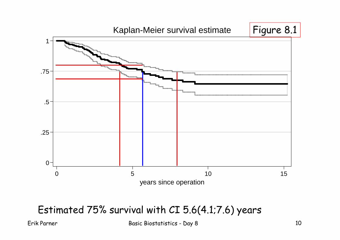
Kaplan-Meier survival estimate

Estimated 75% survival with CI 5.6(4.1;7.6) years

Figure 8.1


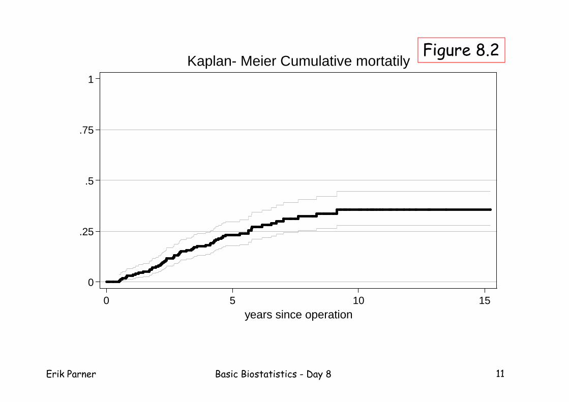
0

.25

.5

.75

1


Kaplan- Meier Cumulative mortatilyFigure 8.2


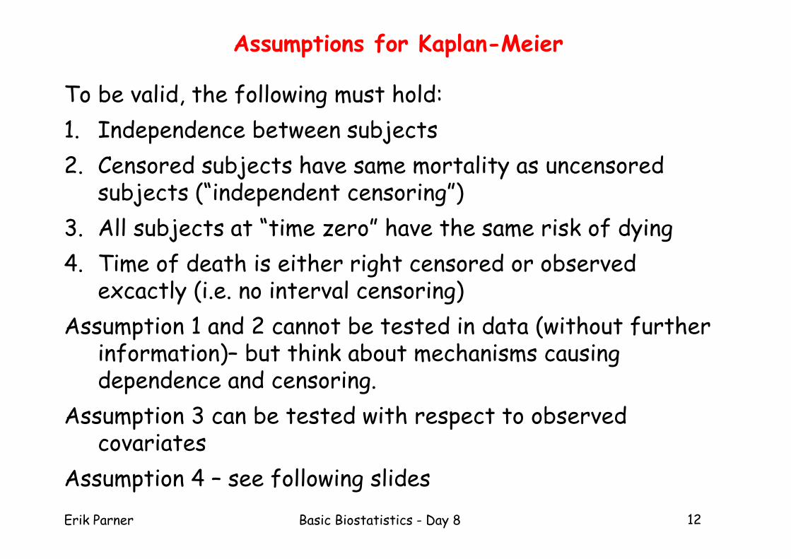
Assumptions for Kaplan-Meier

To be valid, the following must hold:

1. Independence between subjects

2. Censored subjects have same mortality as uncensored subjects (“independent censoring”)

3. All subjects at “time zero” have the same risk of dying

4. Time of death is either right censored or observed excactly (i.e. no interval censoring)

Assumption 1 and 2 cannot be tested in data (without further information)– but think about mechanisms causing dependence and censoring.

Assumption 3 can be tested with respect to observed covariates

Assumption 4 – see following slides


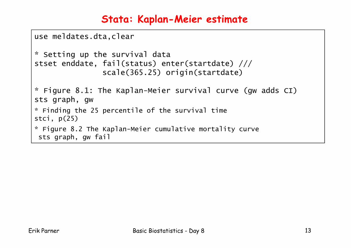
Stata: Kaplan-Meier estimate

use meldates.dta,clear

* Setting up the survival datastset enddate, fail(status) enter(startdate) ///

scale(365.25) origin(startdate)

* Figure 8.1: The Kaplan-Meier survival curve (gw adds CI)sts graph, gw

* Finding the 25 percentile of the survival timestci, p(25)

* Figure 8.2 The Kaplan-Meier cumulative mortality curvests graph, gw fail


Warning when using the Kaplan-Meier methodInterval censored data

The Kaplan-Meier method only works with right censoring.

The method will not work if some of the data is interval censored.

That is, the exact time of event (e.g. death event) is not known – it is only known that the event occurred in a given time interval, e.g. during a two-year period.

Interval censored data is not uncommon in health:

• The patient had a silent AMI between two control-visits.

• A tooth erupted between two visits at the dentist.

• Ect…

The estimation of the survival function under interval censoring is complicated and not included in standard software.


An example of interval censored data A study of reoccurrence of symptoms

The settingIn order to estimate the reoccurrence of symptoms after the operation for incontinence by Burch method, 912 women operated in the period 1974-1993 were mailed a questionnaire in 1993.

The central question was: Have the problems reoccurred since the operation?

Here it is important to note that the (former) patient is not asked when the problem reoccurred – she would probably not be able to offer a precise answer to such a question.

This data will be interval censored as we do not know when the event has happened, only that it happened somewhere in the interval from operation and until the woman answered the question.


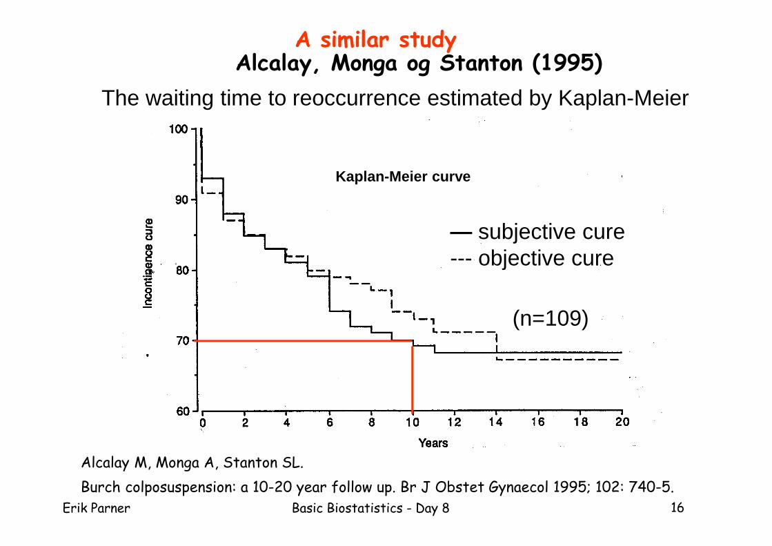
The waiting time to reoccurrence estimated by Kaplan-Meier

Alcalay, Monga og Stanton (1995)

— subjective cure --- objective cure

Kaplan-Meier curve

(n=109)

A similar study

Alcalay M, Monga A, Stanton SL.

Burch colposuspension: a 10-20 year follow up. Br J Obstet Gynaecol 1995; 102: 740-5.


Pro

potio

n w

ithou

t sid

e ef

fect

s

0 5 10 15 20 25

0.0

0.2

0.4

0.6

0.8

1.0

Kaplan-Meier

Turnbull

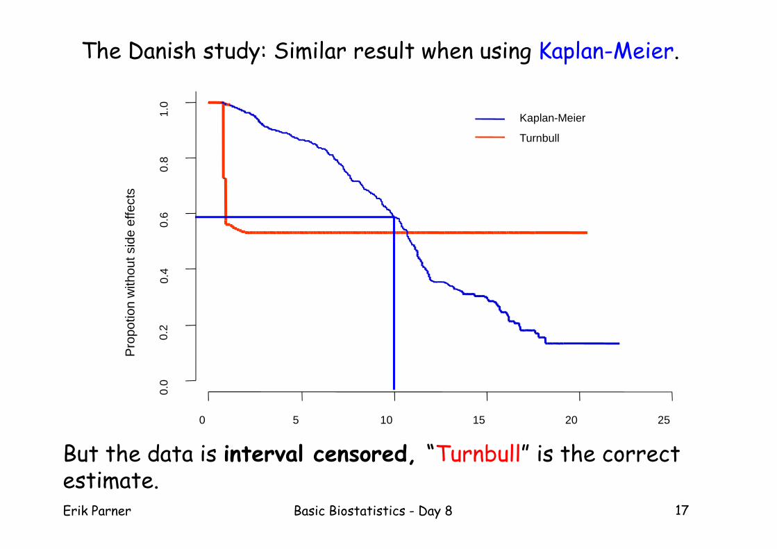
The Danish study: Similar result when using Kaplan-Meier.

But the data is interval censored, “Turnbull” is the correct estimate.


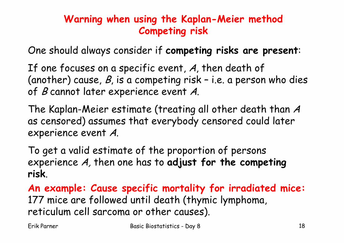
Warning when using the Kaplan-Meier methodCompeting risk

One should always consider if competing risks are present:

If one focuses on a specific event, A, then death of (another) cause, B, is a competing risk – i.e. a person who dies of B cannot later experience event A.

The Kaplan-Meier estimate (treating all other death than Aas censored) assumes that everybody censored could later experience event A.

To get a valid estimate of the proportion of persons experience A, then one has to adjust for the competing risk.

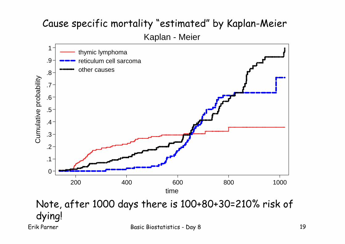
An example: Cause specific mortality for irradiated mice:177 mice are followed until death (thymic lymphoma, reticulum cell sarcoma or other causes).


0

.1

.2

.3

.4

.5

.6

.7

.8

.9

1

Cum

ulat

ive

prob

abili

ty

200 400 600 800 1000time

thymic lymphomareticulum cell sarcomaother causes

Kaplan - Meier

Cause specific mortality “estimated” by Kaplan-Meier

Note, after 1000 days there is 100+80+30=210% risk of dying!


0

.1

.2

.3

.4

.5

.6

.7

.8

.9

1

Cum

ulat

ive

prob

abili

ty

200 400 600 800 1000time

thymic lymphomareticulum cell sarcomaother causes

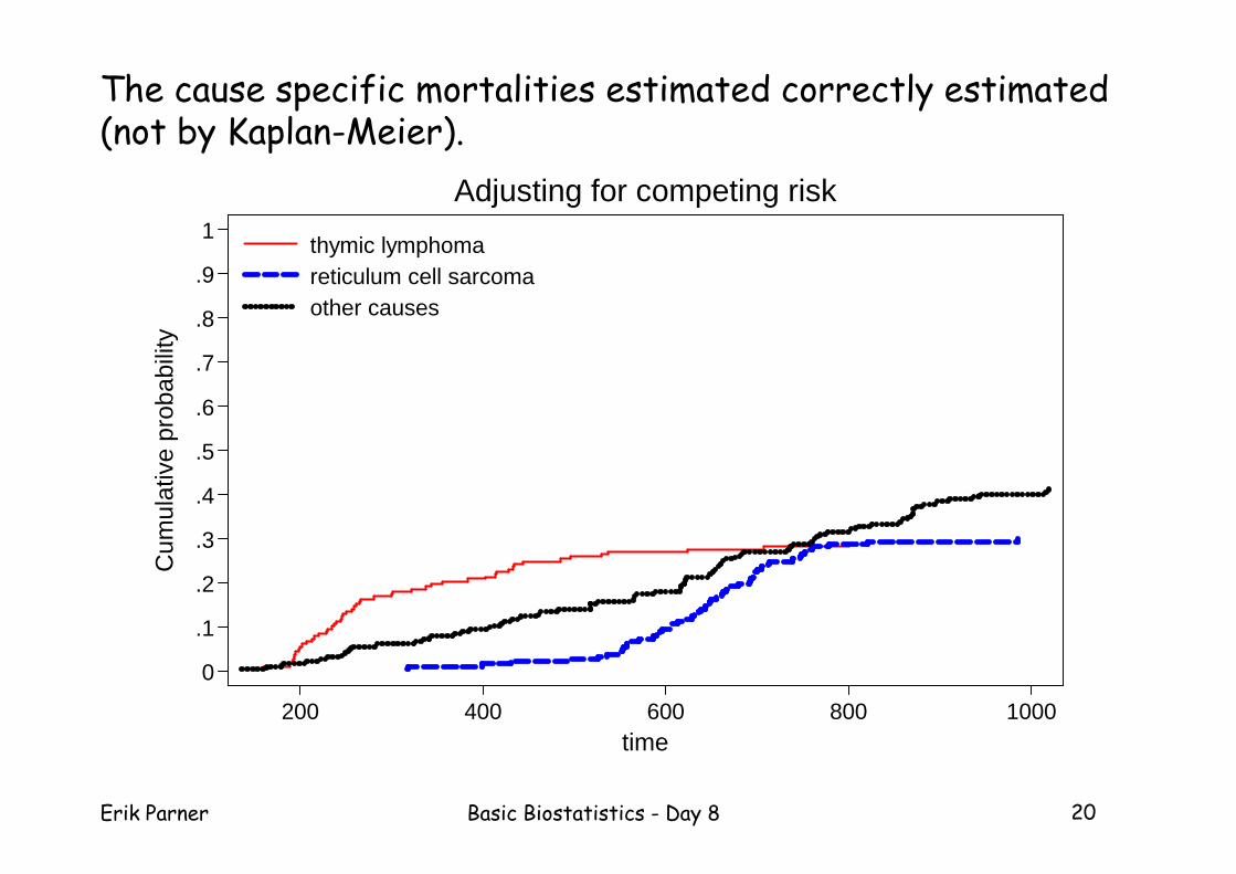
Adjusting for competing risk

The cause specific mortalities estimated correctly estimated (not by Kaplan-Meier).


0.00

0.25

0.50

0.75

1.00


sex = femalesex = male

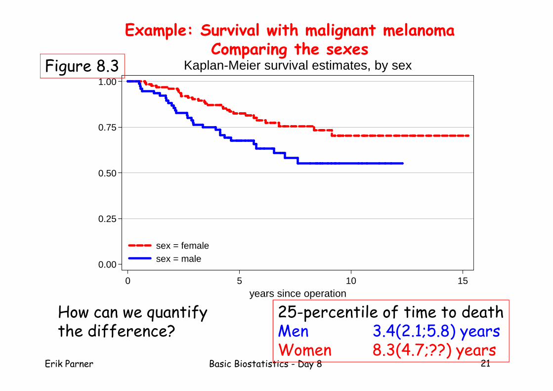
Kaplan-Meier survival estimates, by sex

Example: Survival with malignant melanomaComparing the sexes

How can we quantify the difference?

25-percentile of time to deathMen 3.4(2.1;5.8) yearsWomen 8.3(4.7;??) years

Figure 8.3


Comparing survival in groups:the log-rank test

0.00

0.25

0.50

0.75

1.00



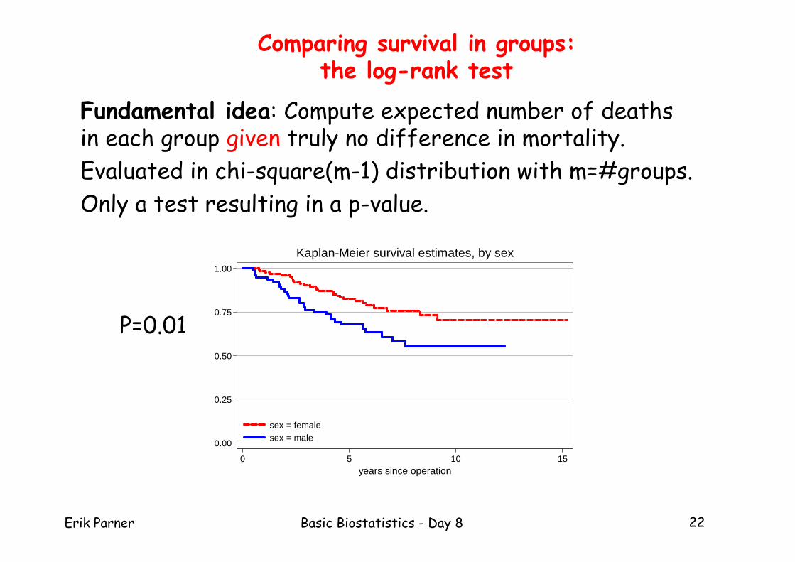
Kaplan-Meier survival estimates, by sex

Fundamental idea: Compute expected number of deaths in each group given truly no difference in mortality.

Evaluated in chi-square(m-1) distribution with m=#groups.

Only a test resulting in a p-value.

P=0.01


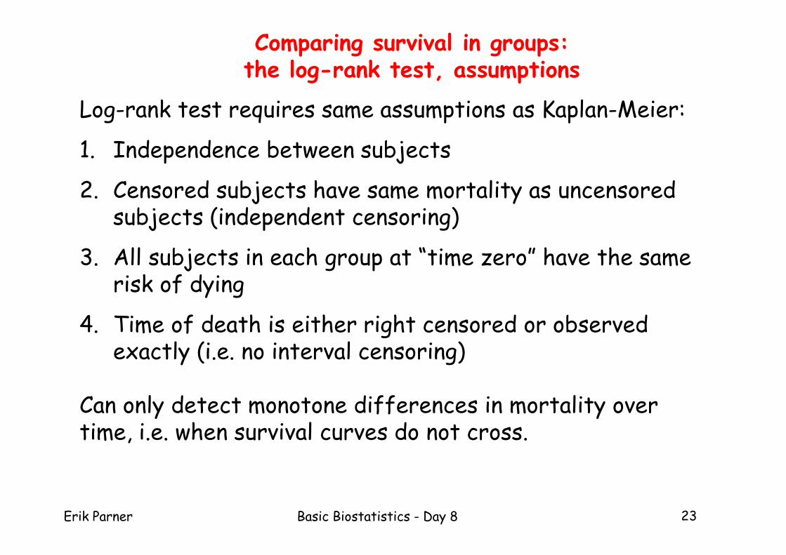
Comparing survival in groups:the log-rank test, assumptions

Log-rank test requires same assumptions as Kaplan-Meier:

1. Independence between subjects

2. Censored subjects have same mortality as uncensored subjects (independent censoring)

3. All subjects in each group at “time zero” have the same risk of dying

4. Time of death is either right censored or observed exactly (i.e. no interval censoring)

Can only detect monotone differences in mortality over time, i.e. when survival curves do not cross.


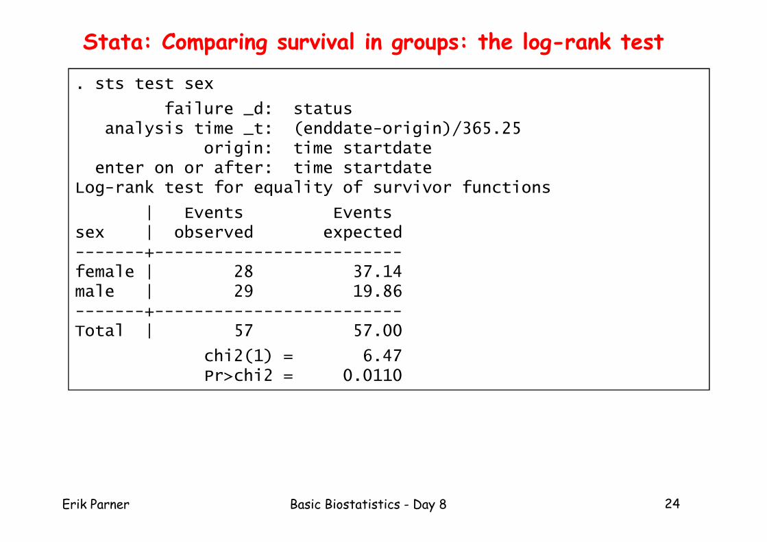
Stata: Comparing survival in groups: the log-rank test

. sts test sex

failure _d: statusanalysis time _t: (enddate-origin)/365.25

origin: time startdateenter on or after: time startdate

Log-rank test for equality of survivor functions

| Events Eventssex | observed expected-------+-------------------------female | 28 37.14male | 29 19.86-------+-------------------------Total | 57 57.00

chi2(1) = 6.47Pr>chi2 = 0.0110


,1,2,5125

102050

100200500

Mor

talit

y ra

te p

er 1

000

year

0 20 40 60 80 100Age

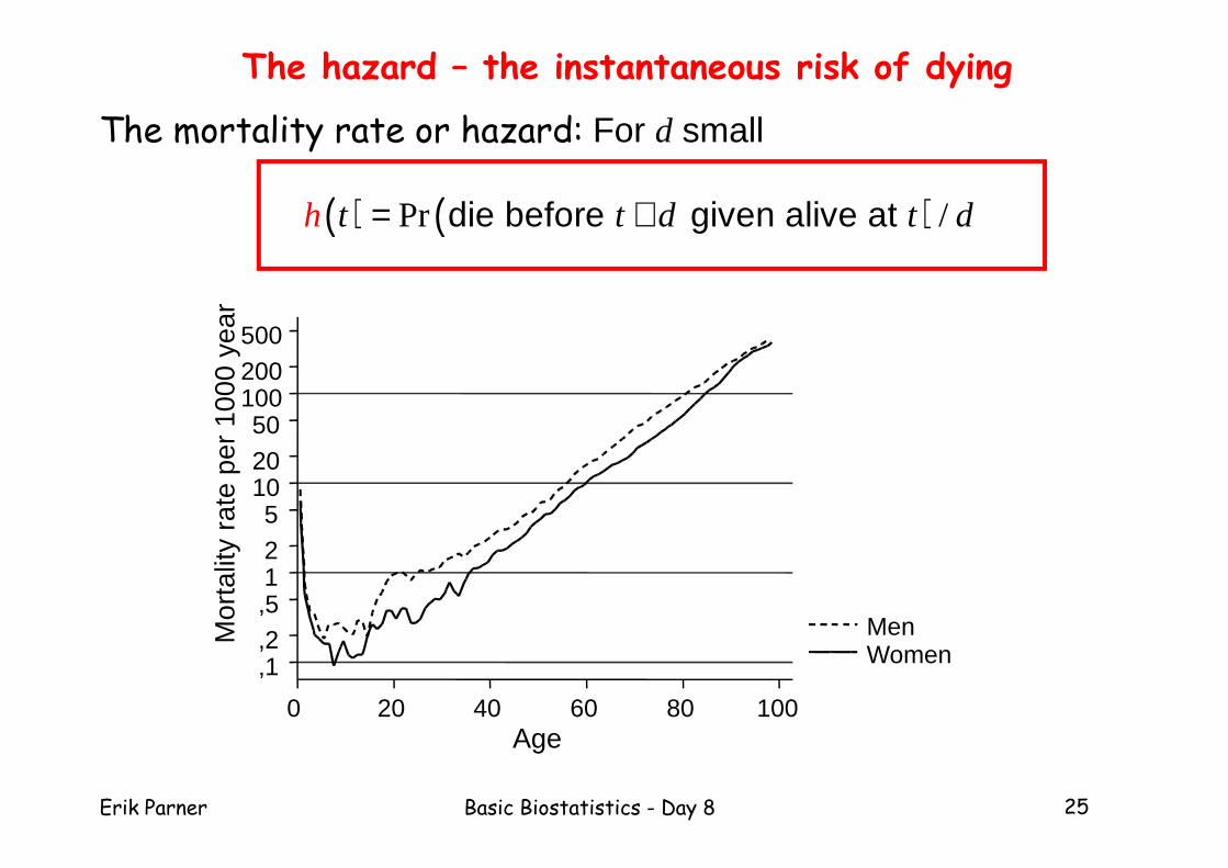
MenWomen

( ) ( )Pr /die before given alive at = +t dh t t d

The mortality rate or hazard: For d small

The hazard – the instantaneous risk of dying


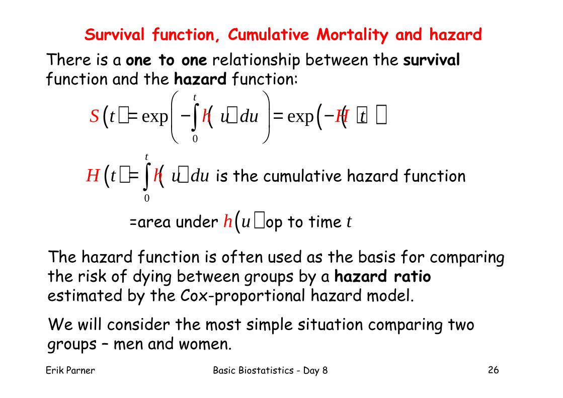
Survival function, Cumulative Mortality and hazard

There is a one to one relationship between the survivalfunction and the hazard function:

( ) ( ) ( )( )0

exp expt

S u duht tH

= − = − ∫

( ) ( )

( )0

= ∫ is the cumulative hazard function

=area under op to time

t

t u du

u

H h

h t

The hazard function is often used as the basis for comparing the risk of dying between groups by a hazard ratioestimated by the Cox-proportional hazard model.

We will consider the most simple situation comparing two groups – men and women.


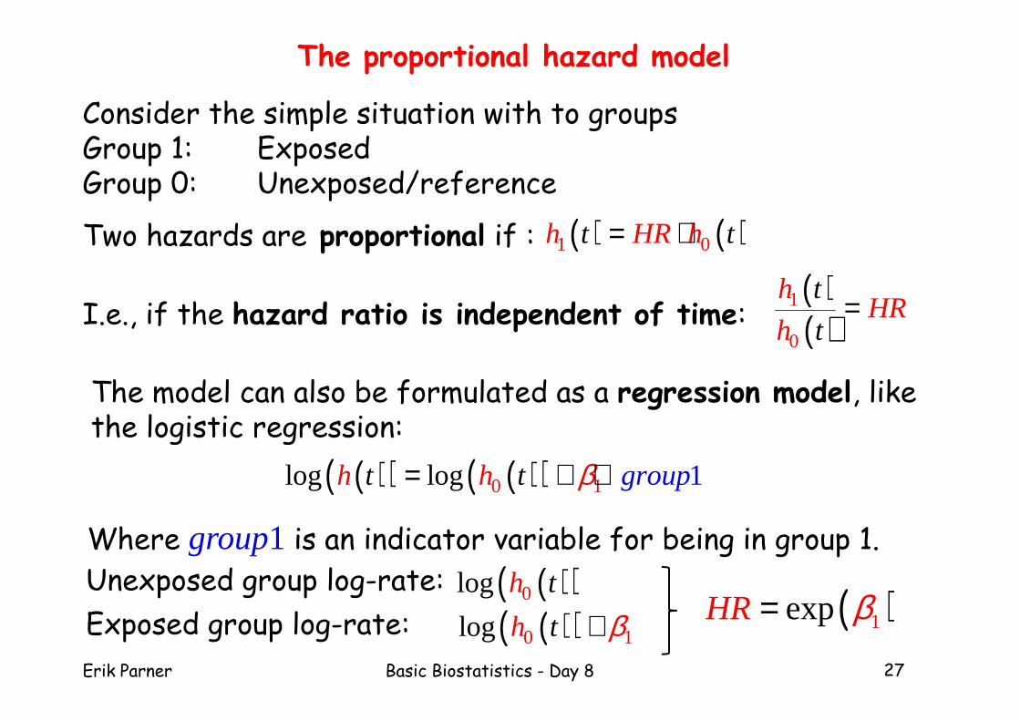
The proportional hazard model

Consider the simple situation with to groupsGroup 1: ExposedGroup 0: Unexposed/reference

Two hazards are proportional if : ( ) ( )1 0h HRt th= ⋅

I.e., if the hazard ratio is independent of time:( )( )

1

0

th

h tHR=

The model can also be formulated as a regression model, like the logistic regression:

( )( ) ( )( )0 1g 1lo logt t gr uph h oβ= + ⋅

Where group1 is an indicator variable for being in group 1.

Unexposed group log-rate: ( )( )0log h t

Exposed group log-rate: ( )( )0 1log β+h t ( )1expHR β=


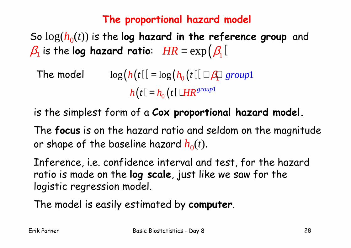
The proportional hazard model

( ) ( )01= ⋅ grouph h HRt t

( )( ) ( )( )0 1g 1lo logt t gr uph h oβ= + ⋅The model

is the simplest form of a Cox proportional hazard model.

The focus is on the hazard ratio and seldom on the magnitude

or shape of the baseline hazard h0(t).

Inference, i.e. confidence interval and test, for the hazard ratio is made on the log scale, just like we saw for the logistic regression model.

The model is easily estimated by computer.

So log(h0(t)) is the log hazard in the reference group and

β1 is the log hazard ratio: ( )1expHR β=


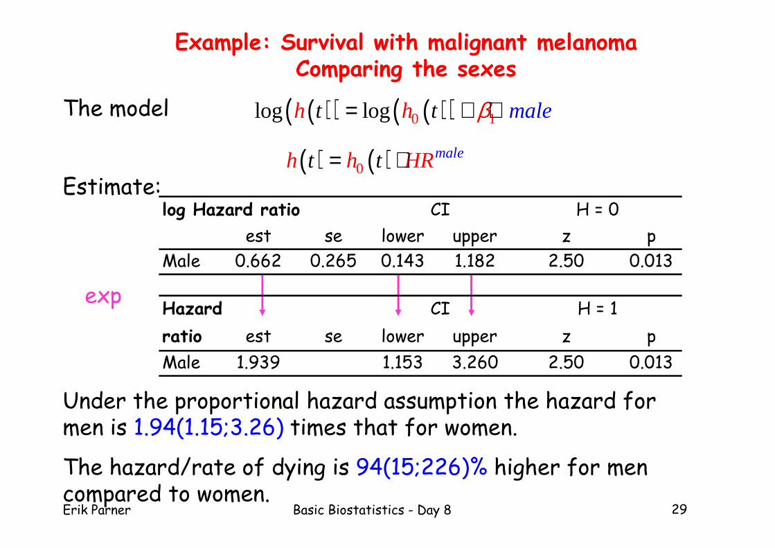
( ) ( )0maleh th HRt = ⋅

( )( ) ( )( )0 1log logt t ah m leh β= + ⋅The model

Under the proportional hazard assumption the hazard for men is 1.94(1.15;3.26) times that for women.

The hazard/rate of dying is 94(15;226)% higher for men compared to women.

Example: Survival with malignant melanomaComparing the sexes

Estimate:

exp

log Hazard ratio

est se lower upper z p

Male 0.662 0.265 0.143 1.182 2.50 0.013

Hazard

ratio est se lower upper z p

Male 1.939 1.153 3.260 2.50 0.013

CI H = 0

CI H = 1


The proportional hazard modelChecking the model

The central assumption is of course that the hazards areproportional, i.e. the hazard ratio does not depend on the time since start.

This assumption can be checked in two ways

1. Plotting the observed survival curves in the two groups together with the estimated survival curves under the model.

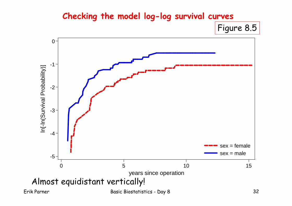
2. A plot of the log-log of the two survival curves.They should be parallel:

( ) ( ) ( ) ( )( )( ) ( ) ( )( )

( )( )( ) ( ) ( )( )( )

1 0 1 0

1 0

1 0

log log log

log log log log log

h HR h H HR H

H HR H

t t t t

t t

t tS HR S

= ⋅ ⇔ = ⋅ ⇔

= + ⇔

− = + −


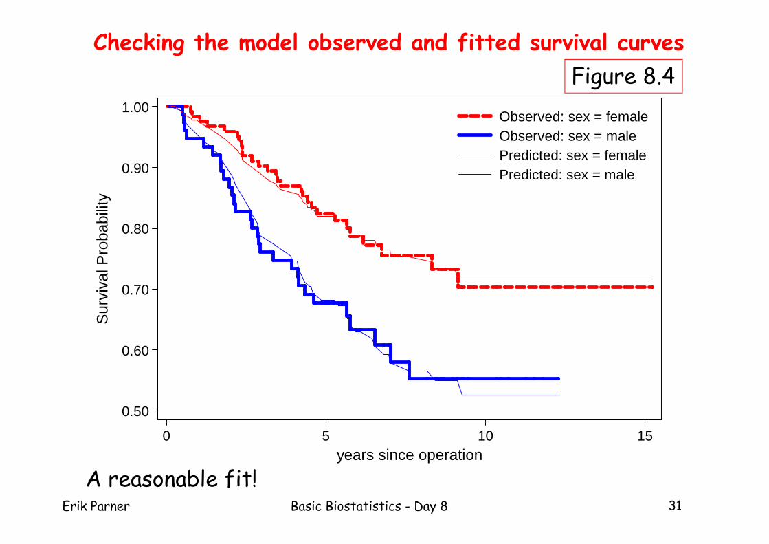
0.50

0.60

0.70

0.80

0.90

1.00S

urvi

val P

roba

bilit

y


Observed: sex = femaleObserved: sex = malePredicted: sex = femalePredicted: sex = male

Checking the model observed and fitted survival curves

A reasonable fit!

Figure 8.4


-5

-4

-3

-2

-1

0ln

[-ln

(Sur

viva

l Pro

babi

lity)

]



Checking the model log-log survival curves

Almost equidistant vertically!

Figure 8.5


0.00

0.20

0.40

0.60

0.80

1.00S

urvi

val P

roba

bilit

y

0 5 10 15 20 25years since cancer

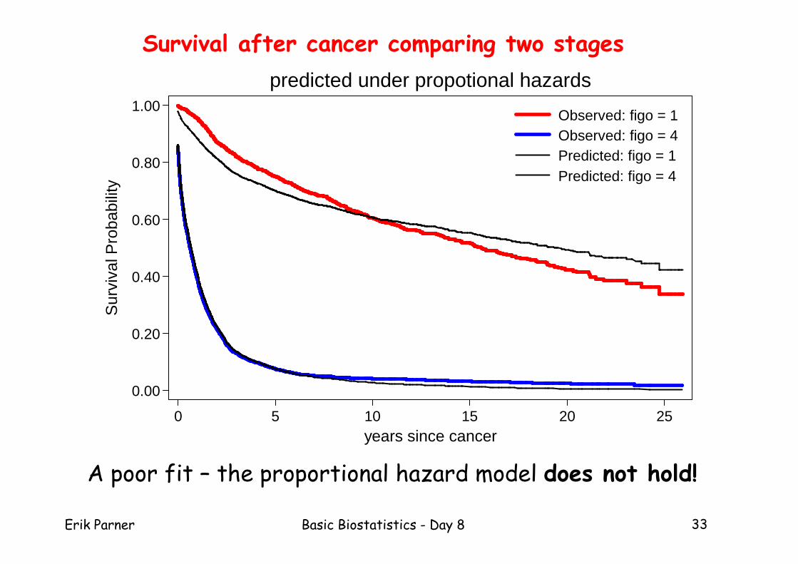
Observed: figo = 1Observed: figo = 4Predicted: figo = 1Predicted: figo = 4

predicted under propotional hazards

Survival after cancer comparing two stages

A poor fit – the proportional hazard model does not hold!


-6

-4

-2

0

2

ln[-

ln(S

urvi

val P

roba

bilit

y)]

0 5 10 15 20 25years since cancer

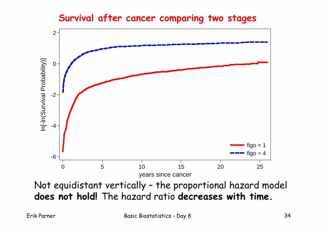
figo = 1figo = 4

Not equidistant vertically – the proportional hazard model does not hold! The hazard ratio decreases with time.

Survival after cancer comparing two stages


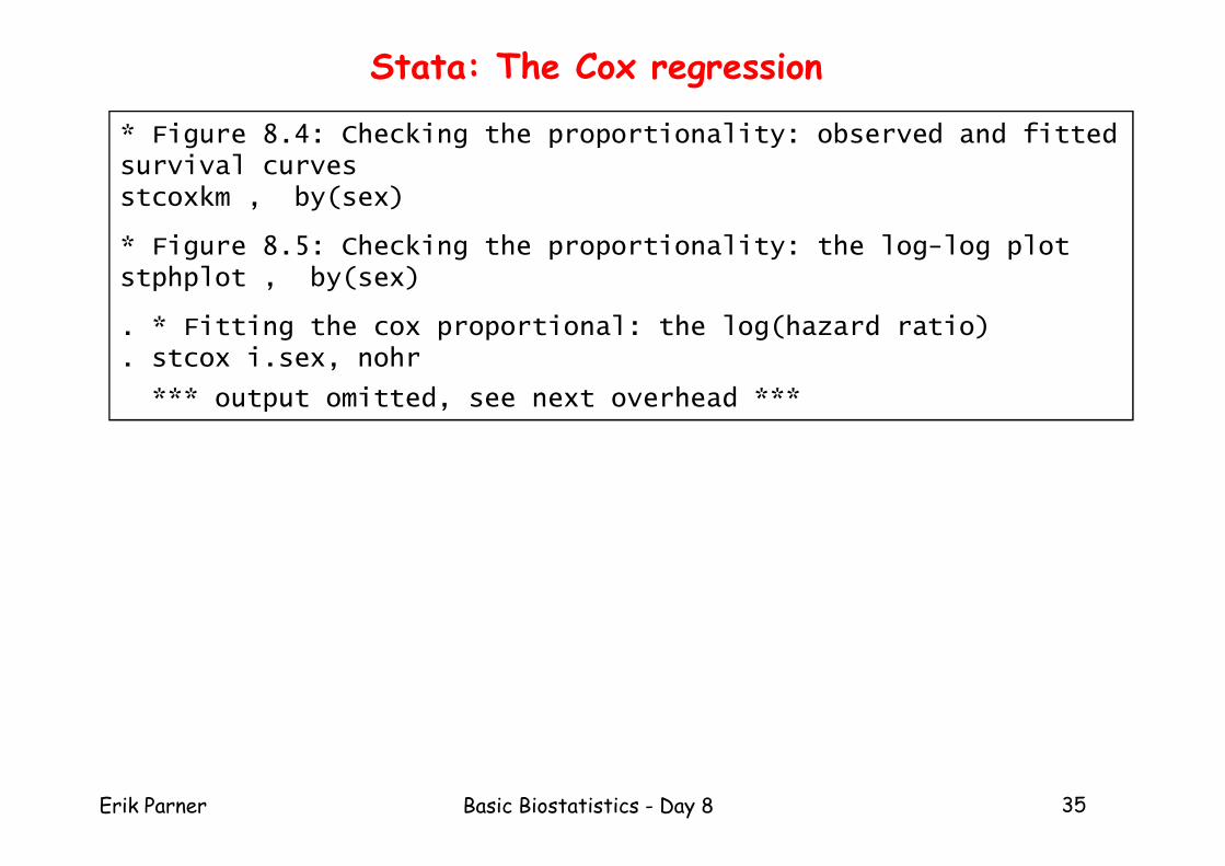
Stata: The Cox regression

* Figure 8.4: Checking the proportionality: observed and fitted survival curvesstcoxkm , by(sex)

* Figure 8.5: Checking the proportionality: the log-log plotstphplot , by(sex)

. * Fitting the cox proportional: the log(hazard ratio)

. stcox i.sex, nohr

*** output omitted, see next overhead ***


Stata: The Cox regression

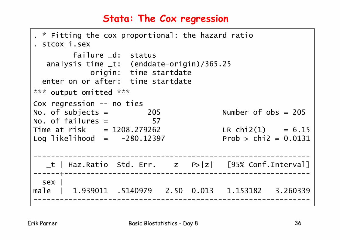
. * Fitting the cox proportional: the hazard ratio

. stcox i.sex

failure _d: statusanalysis time _t: (enddate-origin)/365.25

origin: time startdateenter on or after: time startdate

*** output omitted ***

Cox regression -- no tiesNo. of subjects = 205 Number of obs = 205No. of failures = 57 Time at risk = 1208.279262 LR chi2(1) = 6.15Log likelihood = -280.12397 Prob > chi2 = 0.0131

---------------------------------------------------------------_t | Haz.Ratio Std. Err. z P>|z| [95% Conf.Interval]

------+--------------------------------------------------------sex |

male | 1.939011 .5140979 2.50 0.013 1.153182 3.260339---------------------------------------------------------------


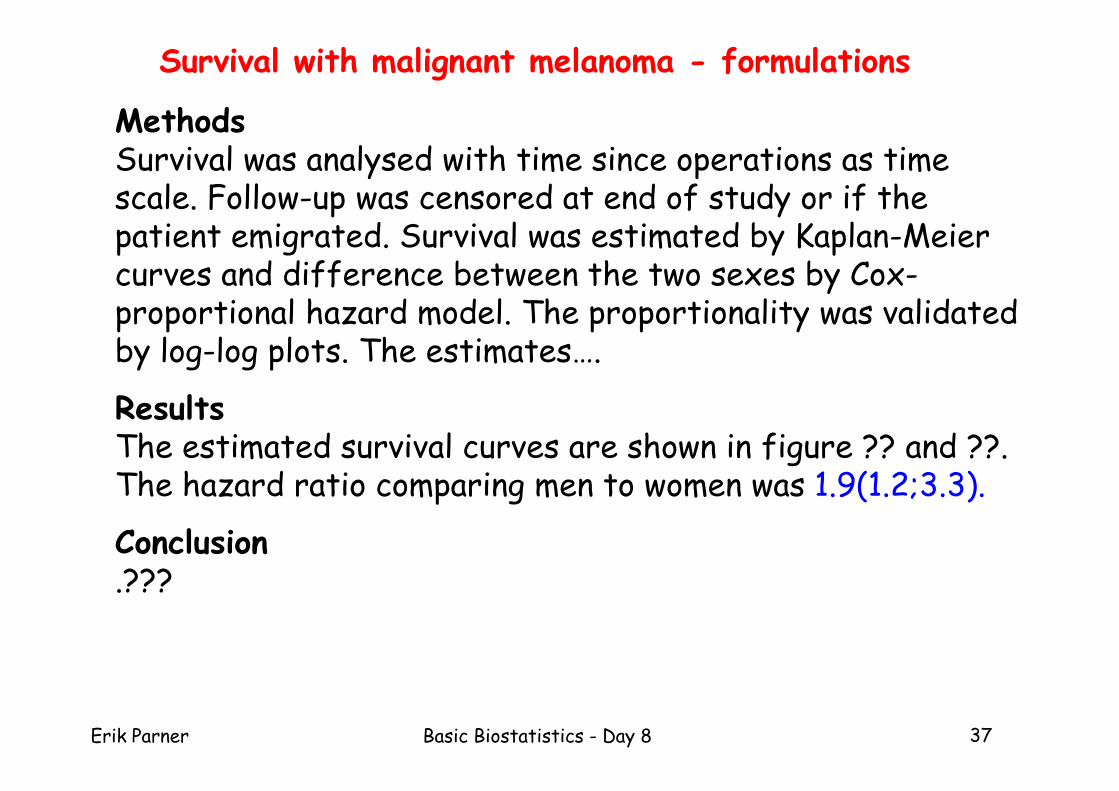
Survival with malignant melanoma - formulations

MethodsSurvival was analysed with time since operations as time scale. Follow-up was censored at end of study or if the patient emigrated. Survival was estimated by Kaplan-Meier curves and difference between the two sexes by Cox-proportional hazard model. The proportionality was validated by log-log plots. The estimates….

ResultsThe estimated survival curves are shown in figure ?? and ??. The hazard ratio comparing men to women was 1.9(1.2;3.3).

Conclusion.???


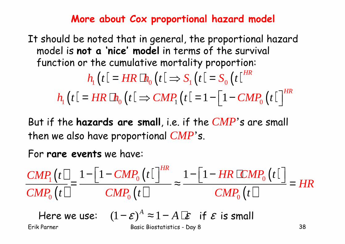
More about Cox proportional hazard model

It should be noted that in general, the proportional hazard model is not a ‘nice’ model in terms of the survival function or the cumulative mortality proportion:

( ) ( ) ( ) ( )1 0 1 0

HRt t th HR h tS S= ⋅ ⇒ =

( ) ( ) ( ) ( )1 0 01 1 1HR

h HR h CMP Ct t t tMP = ⋅ ⇒ = − −

But if the hazards are small, i.e. if the CMP’s are small

then we also have proportional CMP’s.

For rare events we have:

( )( )

( )( )

( )( )

0 01

0 0 0

1 1 1 1HR

CMP HR CMPCMPHR

CMP CMP

t tt

t t tCMP

− − − − ⋅ = ≈ =

(1 ) 1 if is small A Aε ε ε− ≈ − ⋅Here we use:


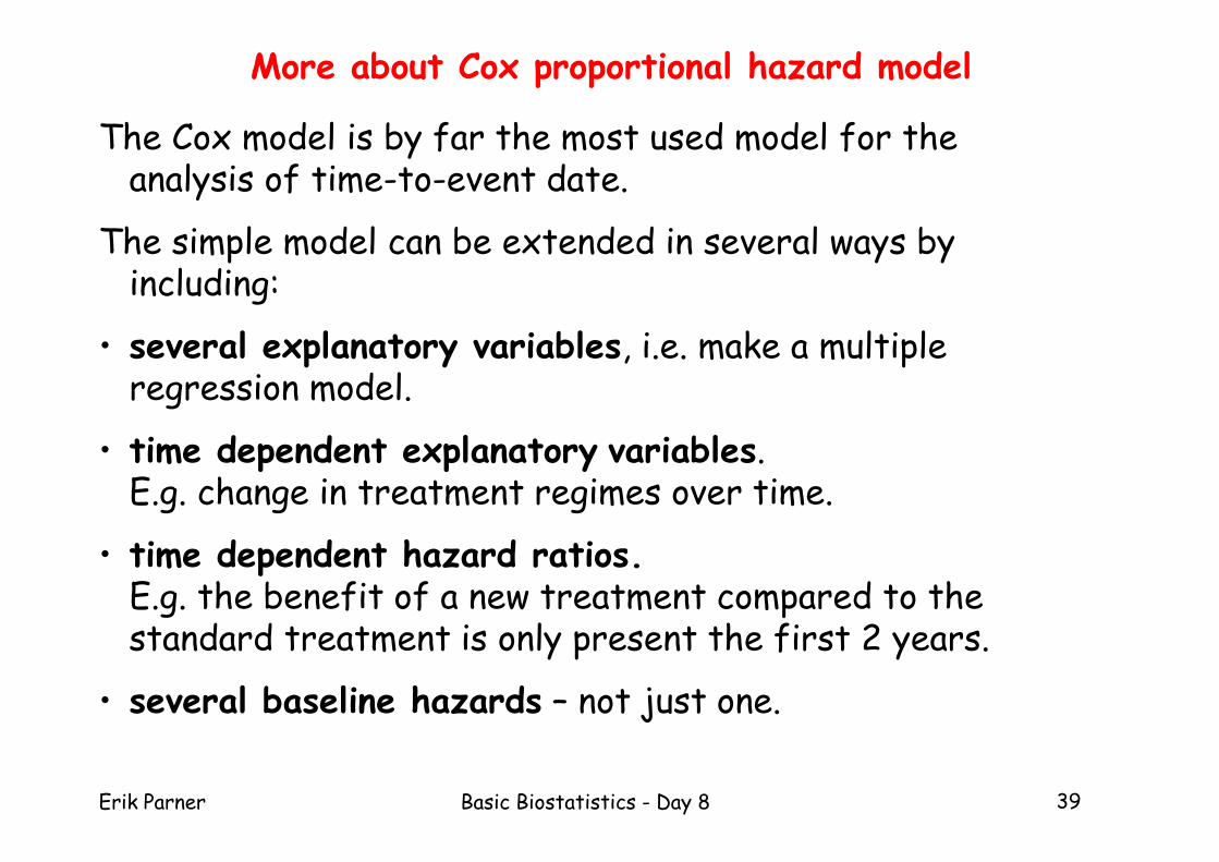
More about Cox proportional hazard model

The Cox model is by far the most used model for the analysis of time-to-event date.

The simple model can be extended in several ways by including:

• several explanatory variables, i.e. make a multiple regression model.

• time dependent explanatory variables. E.g. change in treatment regimes over time.

• time dependent hazard ratios. E.g. the benefit of a new treatment compared to the standard treatment is only present the first 2 years.

• several baseline hazards – not just one.

Documents

Erik Parner, Department of Biostatistics, Aarhus University©