Embed Size (px)
Citation preview
es Pump Efficiency Solutions
Pump Sequencing Optimization
by
John F. Allan
Kyle J. Nekimken
Spencer B. Weills
Mechanical Engineering Department
California Polytechnic State University
San Luis Obispo
2009

es Pump Efficiency Solutions
ii
Statement of Disclaimer
Since this project is a result of a class assignment, it has been graded and accepted as fulfillment of the course requirements. Acceptance does not imply technical accuracy or reliability. Any use of information in this report is done at the risk of the user. These risks may include catastrophic failure of the device or infringement of patent or copyright laws. California Polytechnic State University at San Luis Obispo and its staff cannot be held liable for any use or misuse of the project.
es Pump Efficiency Solutions
i
Table of Contents Statement of Disclaimer ............................................................................................................................... ii List of Figures ................................................................................................................................................ 1 List of Tables ................................................................................................................................................. 1 Abstract ......................................................................................................................................................... 2 Introduction .................................................................................................................................................. 3
Formal Problem Definition ........................................................................................................................ 3 Objectives ................................................................................................................................................. 3 Project Management Plan ........................................................................................................................ 4
Background ................................................................................................................................................... 5 Current State of the Art ............................................................................................................................ 5 Types of Systems ....................................................................................................................................... 5
Modeling ....................................................................................................................................................... 8 Requirements ............................................................................................................................................ 8 Conceptualization ................................................................................................................................... 10 Verification of Model .............................................................................................................................. 12
Design Development ................................................................................................................................... 15 Program Overview ...................................................................................................................................... 15
Sample Analysis ....................................................................................................................................... 17 Final Design ................................................................................................................................................. 19 Governing Pumping Equations.................................................................................................................... 19
MATLAB™ Program ................................................................................................................................. 19 MATLAB™ To Trane Graphical Programming (TGP) ................................................................................ 20 Technician Implementation .................................................................................................................... 21 Program Design and Debugging .............................................................................................................. 22
Conclusions ................................................................................................................................................. 23 References .................................................................................................................................................. 24 Appendices .................................................................................................................................................. 25
Appendix A: QFD ..................................................................................................................................... 25 Appendix B: List of Vendors .................................................................................................................... 26 Appendix C: Vendor Supplied Component Specifications and Data Sheets ........................................... 27 Appendix D: Programming Code ............................................................................................................. 28
MATLAB™ ............................................................................................................................................ 28 TGP ...................................................................................................................................................... 30
Appendix E: Gantt Charts ........................................................................................................................ 31
es Pump Efficiency Solutions
1
List of Figures
Figure 1. Primary-Secondary System ............................................................................................................ 6
Figure 2. Variable Flow System Model ........................................................................................................ 10
Figure 3. Peerless 8AE20 17" Pump Curve .................................................................................................. 11
Figure 4. Darcy-Weisbach Equation ............................................................................................................ 11
Figure 5. CVHF Evaporator Head Loss Curve .............................................................................................. 11
Figure 6. Performance Curve for Two Parallel Pump System ..................................................................... 12
Figure 7. PSIM Model .................................................................................................................................. 13
Figure 8. PSIM System and Pump Curves ................................................................................................... 14
Figure 9. Program Flowchart ....................................................................................................................... 15
Figure 10. Swamee-Jain equation for friction factor with turbulent flow .................................................. 16
Figure 11. Pump efficiency equation .......................................................................................................... 17
Figure 12. Sample Pump and System Curves .............................................................................................. 17
Figure 13: Operating Flow Rate Calculation in MATLAB™ code ................................................................. 20
Figure 14: Operating Flow Rate in TGP (Partial Diagram) ........................................................................... 21
Figure 15: Trane UM 4160 Chiller/Evaporator Curve ................................................................................ 27
Figure 16. Peerless 8AE20 17" Pump Curve ................................................................................................ 28
Figure 17. Winter 09 Gantt Chart ............................................................................................................... 31
Figure 18. Spring 09 Gantt Chart ................................................................................................................ 32
Figure 19. Fall 09 Gantt Chart ..................................................................................................................... 33
List of Tables
Table 1. Optimization results for a VFD pump compared to a constant speed pump. .............................. 18
Table 2-QFD (House of Quality) .................................................................................................................. 26
es Pump Efficiency Solutions
2
Abstract
The purpose of this document is to demonstrate the design, production, and testing of optimum pump
sequencing logic for variable frequency drive (VFD) pumps in commercial heating ventilating and air
conditioning (HVAC) systems. The product will be developed by Pump Efficiency Solutions (PES), which is
a group of Cal Poly students working on their senior project. The product is being developed for Trane,
an industry leader in large scale HVAC systems. MATLAB™, Microsoft Excel, Pump System Improvement
Modeling Tool™ (PSIM), and fluid mechanics hand calculations were used during software development.
Next, we converted the program into Trane’s graphical programming language (TGP) and applied these
algorithms to a MP580 Controller.
There were three separate phases to the project. The phases, each lasting one quarter, can be
designated as conceptualizing, modeling, and programming. During the design conceptualizing PES
gathered information on commercial HVAC systems and VFD pumps which can be implemented into
these systems. We then modeled a simple system using PSIM and developed a series of optimization
algorithms within excel to optimize the quantity of the pumps for a given system load (flow-rate) and
pressure requirements. The completion of the model represented the end of the conceptualizing phase
and beginning of the modeling phase.
For the second phase of the project, we took the analysis from Excel and used it to develop a general
algorithm which can be applied to a variety of different systems. Essentially, it incorporates pump curves
for the specific pumps selected for a system and calculates the theoretical best number of pumps to run
for maximum system energy efficiency at a given load. This algorithm can be adaptable to any system
and will be incorporated into Trane’s pre-existing system control software. The program will have
permanent inputs based on the components and geometry of the system in addition to dynamic inputs
that define the current operating conditions due to a transient load. The outputs of the program will be
number of pumps that should run in order to match the load and minimize power consumption.
In the programming phase, we translated our MATLAB™ program into a series TGP files to make the
algorithms compatible with the controller. To simulate changes in system head and flow rate, we
connected two potentiometers to the controller. Both MATLAB™ code and MP580 controller simulation
successfully calculated the optimum number of pumps to operate given any system inputs within a
standard operating range.
es Pump Efficiency Solutions
3
Introduction
First off, let us introduce ourselves as Pump Efficiency Solutions. We are a group of three Cal Poly M.E.
students who are working together on our senior project. During this yearlong project, we studied pump
sequencing and optimization as specified by Trane and our university, California Polytechnic State
University San Luis Obispo (Cal Poly). Our names are John Allan, Kyle Nekimken, and Spencer Weills.
Formal Problem Definition
The project entails developing a set of algorithms which will maximize efficiency in building cooling
systems. This will be done by optimizing the pumping system for a given load (flow-rate and pressure)
on the water side of an industrial HVAC system. Our end goal is to deliver a set of algorithms which will
be easily applied to multiple buildings by field technicians.
The major stakeholders are Trane, ourselves, and Cal Poly. Trane, because they will invest time and
resources into the project and in turn will receive a practical and functional deliverable. We consider
ourselves stakeholders because aside from being graded on our performance, our reputations are
dependent on the success of this project. Of course Cal Poly has a vested interest because they will not
only contribute resources to the project, but they want to see their students succeed and help the
university’s reputation as one of the leading undergraduate engineering universities in the country.
Objectives
The main objective of this project is to deliver a user friendly, self explanatory, and practical program to
Trane that meets all of the specifications defined in our QFD (Appendix A). These objectives come from
the engineering specifications which are the parameters that need to be met in accordance with our
customer’s requirements.
The program’s main objective is to take, as an input, characteristics of an existing or proposed HVAC
system, including pumps, piping system specifications, and minimum flow and pressure requirements.
The program’s algorithms use the required load with given system parameters to control the number of
operating pumps to meet the required flow rate and operating pressures through the system. Variable
frequency drive (VFD) motors can run at an effectively infinite number of frequency denominations, and
it is assumed that all pumps in the system are driven by VFD’s. Each of these frequencies produces a
different pump curve, which corresponds to a different operating point. The program dynamically scales
the pump curves to maintain the optimum running frequency for the system’s pumps. Additionally, the
program accounts for frictional losses based on the piping and geometric parameters as defined by the
Darcy-Weisbach equation (Figure 5).
The output delivered by the program specifies the number of pumps needed to achieve the lowest
power input while still meeting the flow rate and operating pressure requirements. In a system with
multiple pumps, this is accomplished by optimizing the sequencing of the pumps in such a way as to
es Pump Efficiency Solutions
4
keep each pump closest to its best efficiency point thus lowering the input power to each pump. The
outputs of the program are simply the number of pumps that should be operating the pumps’
frequency. The program must be flexible enough to allow for process variation due to different pump
types which may have significantly different shaped operating curves as well as a wide variety of
detailed variable inputs due to particular pump or chiller characteristics and orientations. If the best way
to optimize a given system is to add an additional pump, then the program should be able to determine
the effect of the new pump. The program must also clearly specify the required input variables
The program (or associated documentation) must clearly and completely demonstrate the physical
principles upon which the program relies. The program should be able to produce dynamic performance
curves and clear, useful, results as the number of pumps, the system load, and operating pressure
requirements change. Any assumptions inherent to the calculations must be stated. Any background
information that the user may need should be listed as well.
The program must easily interface with Building Automation Systems (BAS), which is Trane’s user
interface program. A technician should be able to look at a graphical building design, easily input the
variables into the program, and get results back without any difficulty. For this to be possible, the
program must be easily navigable and the input process must follow a logical path. Further, the results
produced must be provided in a clear and concise manner to avoid confusion.
Though industrial HVAC systems involve a significant amount of thermal analysis, our project is more
focused on the water side of the system (more specifically the pumps). Thus we are not focusing on the
heat transfer occurring in the system. Instead we are concentrating more on the fluid-dynamics side of
system modeling and defining our water side load as the flow rate required by the overall system to
deliver proper flow rate.
Project Management Plan
The project can be divided into four main sections: researching, modeling, programming, and
implementation. Although the project is a collaborative effort, each group member had specific tasks he
coordinated. Background research was shared equally between all three members since it was
important for everyone to have an understanding of chilled water systems. Additionally, writing and
editing reports was a collaborative effort. For the remaining tasks, Kyle Nekimken was in charge of the
modeling segment, Spencer Weills oversaw programming, and John Allan coordinated the
implementation. For each subsystem, the leader acted like the project manager while the other two
members were supporting engineers helping to implement each task. Our preliminary schedules,
including deadlines for our deliverables, are in Appendix E in the form of Gantt Charts.
es Pump Efficiency Solutions
5
Background
In this day and age of limited energy resources, the need and demand for improved efficiency in
industrial HVAC systems is growing exponentially since these systems account for a large fraction of
total energy usage. In the United States, our total annual energy consumption was approximately 100
quads (1015 BTU) in 2006 according to the U.S. Department of Energy. Of this energy, 40% was
consumed by buildings with about 1/3 of this powering the HVAC system. This brings the energy to
around 13 quads. Within HVAC systems, about 40% of this energy is spent on pumping. This means that
about 5x10¹⁵ BTU of energy is spent solely to run HVAC pumps. Therefore any improvements in pump
system efficiency will have a significant on overall energy consumption. One of the most simple, but still
intricate, ways to improve efficiency is through pump sequencing optimization.
Pump sequencing basically defines how many pumps should operate to achieve maximum energy
efficiency, while still maintaining the desired system performance. As far as VFD pumping goes, this
means pump sequencing and speed regulation. Since there are an infinite number of operating speeds,
it is essential that the pump is managed such that the system is always at the most efficient level.
Current State of the Art
Designing a pump sequencing optimization method is something that has been addressed before. There
are already a small number of black box systems and field programmed systems available for purchase
from HVAC companies. However, none of these systems have verifiable evidence to support their claims
of energy efficiency. The companies that do offer products only claim increased efficiency, but they do
not offer any sort of documented evidence which illustrates how they make the system more efficient
nor to what extent they are more efficient. Surprisingly enough, the HVAC industry as a whole has left
the topic of our project very lightly explored. As energy efficiency has become even more important in
light of the current energy crisis, more companies are looking for ways to improve their HVAC systems.
In an industrial cooling system, pumps use a large fraction of the total energy expended, which further
highlights the need for improved pumping controls.
We plan defined a set of adaptable algorithms to work for a variety of industrial cold water systems. To
accomplish this, we first researched pump systems and then came up with a set of algorithms based on
pump efficiency curves and governing equations. The scope of our project does not include the chiller
operation, heat transfer optimization, or any airside components of HVAC systems.
Types of Systems
The industry has significant experience with Primary-Secondary chilled water systems. These chilled
water systems are arranged using two loops as illustrated in Figure 1 below. The primary loop contains
chillers which are sequenced on and off as the load rises and falls. When a chiller is operating, it is
provided with a constant chilled water flow (gpm) regardless of the required cooling load (tons).
The secondary loop has separate pumps which only provide enough pressure to induce the required
flow though the distribution system, cooling coil, control valves and other system accessories. In a
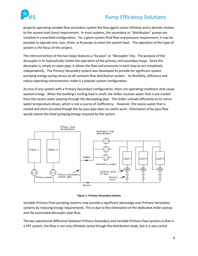
es Pump Efficiency Solutions
6
properly operating variable flow secondary system the flow (gpm) varies infinitely and is directly related
to the system load (tons) requirement. In most systems, the secondary or “distribution” pumps are
installed in a manifold configuration. For a given system fluid flow and pressure requirement, it may be
possible to operate one, two, three, or N pumps to meet the system load. The operation of this type of
system is the focus of this project.
The interconnection of the two loops features a “by-pass” or “decoupler’ line. The purpose of the
decoupler is to hydraulically isolate the operation of the primary and secondary loops. Since the
decoupler is simply an open pipe, it allows the flow and pressures in each loop to act completely
independently. The Primary-Secondary system was developed to provide for significant system
pumping energy saving versus an all constant flow distribution system. Its flexibility, efficiency and
robust operating characteristics make it a popular system configuration.
As true of any system with a Primary-Secondary configuration, there are operating conditions that cause
wasted energy. When the building’s cooling load is small, the chiller receives water that is pre-cooled
from the excess water passing through the decoupling pipe. The chiller unloads efficiently as its return
water temperature drops, which is not a source of inefficiency. However, the excess water that is
cooled and short circuited though the by-pass pipe does no useful work. Elimination of by-pass flow
would reduce the total pumping energy required by the system.
Figure 1. Primary-Secondary System
Variable-Primary Flow pumping systems may provide a significant advantage over Primary-Secondary
systems by reducing energy requirements. This is due to the elimination of the dedicated chiller pumps
and the associated decoupler pipe flow.
The key operational difference between Primary-Secondary and Variable Primary Flow systems is that in
a VPF system, the flow is not only infinitely varied though the distribution loads, but it is also varied

es Pump Efficiency Solutions
7
within limits though the chillers. This provides pumping energy savings since the excess by-pass flow is
eliminated at many loads. By-Pass flow is still required at some part load conditions to ensure that the
flow does not drop below the chiller’s minimum allowed flow, which results in laminar flow and
therefore reduced heat transfer. The pumps in a Variable-Primary Flow system are often configured and
operated exactly like the distribution pumps in a Primary-Secondary system. The final outcome of this
project will be directly applicable to this system’s pumping configuration.
es Pump Efficiency Solutions
8
Modeling
Reading through several of Trane’s chiller design documents, we have gained a reasonable
understanding of chilled water cooling systems. In particular we have concentrated our research on the
implementation of VFD pumps within systems. We have studied three different ways to control VFD
pumps: at a constant pressure differential, a constant flow rate, and a variable flow rate. In HVAC
applications, it is most common to use variable flow arrangements because it allows for frequent
fluctuations in the system load. By sequencing the pumps and regulating pump speed, a HVAC system
can achieve lower energy consumption.
The model serves two purposes: to further our comprehension of chilled water systems and to aid us in
determining the necessary parameters to measure when sequencing the pumps. In choosing these
parameters, we will emphasize the simplicity of instrumentation and taking measurements. Providing a
simple method for collecting data meets our objective to create a user friendly program.
Additionally, the model will help us identify ways to optimize energy efficiency. We will calculate system
energy consumption and cooling capacity that corresponds to the optimal pump sequence. This model
will provide a starting point for programming the sequencing code, but we will continue to modify the
model as our project moves forward.
Requirements
In a closed loop pumping system, the pump manifold must produce a sufficient amount of pressure to
maintain circulation. This pressure needs to overcome frictional losses in the system due to piping,
fittings, and a variety of valves. Thus, the pumps must generate a specific pressure drop across the
pump headers based on operating conditions. Control valves at each air handler determine the chilled
water flow rate according to the cooling requirement. For example, when cooling demand is low, the
control valves close thus reducing the flow rate. Likewise, the required pumping pressure decreases
with cooling demand. This variability in operating conditions results in an infinite number of possible
operating points for the pump manifold.
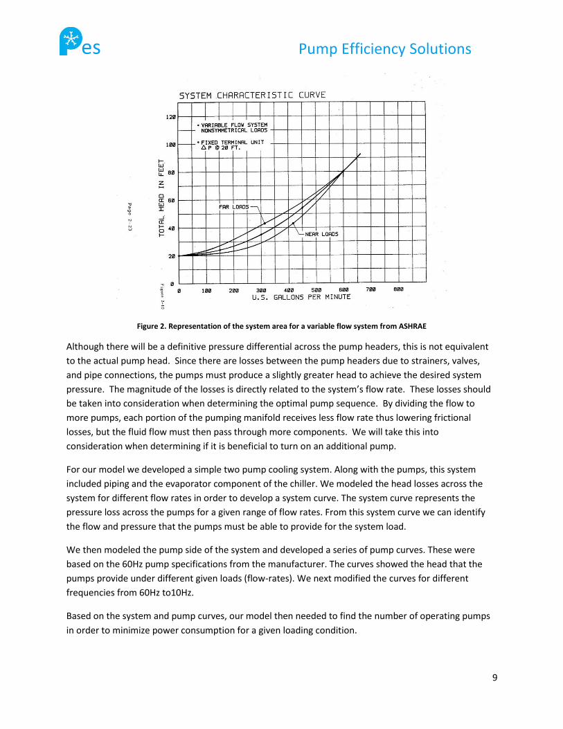
Unlike a simple linear system, a system with multiple control valves will not have a single system curve
to designate the possible operating points. Instead, there is an area containing the set of operating
points that can occur. To determine the boundaries of this area, we eliminated operating points that
cannot occur. First, we calculated the system’s maximum level (when all the control valves are
completely open). Conversely, when there are no control valves the minimum flow rate and head occur.
In between these points the boundary of the system is based on which part of the building requires
chilled water. Cooling loads at the far end of the system define the upper boundary while loads near the
pumps create the lower boundary as shown in Figure 2. The figure does not intersect the origin due to
the frictional losses in the piping that will be present even when the flow rate is zero or minimal through
the airside components.
es Pump Efficiency Solutions
9
Figure 2. Representation of the system area for a variable flow system from ASHRAE
Although there will be a definitive pressure differential across the pump headers, this is not equivalent
to the actual pump head. Since there are losses between the pump headers due to strainers, valves,
and pipe connections, the pumps must produce a slightly greater head to achieve the desired system
pressure. The magnitude of the losses is directly related to the system’s flow rate. These losses should
be taken into consideration when determining the optimal pump sequence. By dividing the flow to
more pumps, each portion of the pumping manifold receives less flow rate thus lowering frictional
losses, but the fluid flow must then pass through more components. We will take this into
consideration when determining if it is beneficial to turn on an additional pump.
For our model we developed a simple two pump cooling system. Along with the pumps, this system
included piping and the evaporator component of the chiller. We modeled the head losses across the
system for different flow rates in order to develop a system curve. The system curve represents the
pressure loss across the pumps for a given range of flow rates. From this system curve we can identify
the flow and pressure that the pumps must be able to provide for the system load.
We then modeled the pump side of the system and developed a series of pump curves. These were
based on the 60Hz pump specifications from the manufacturer. The curves showed the head that the
pumps provide under different given loads (flow-rates). We next modified the curves for different
frequencies from 60Hz to10Hz.
Based on the system and pump curves, our model then needed to find the number of operating pumps
in order to minimize power consumption for a given loading condition.
es Pump Efficiency Solutions
10
Conceptualization
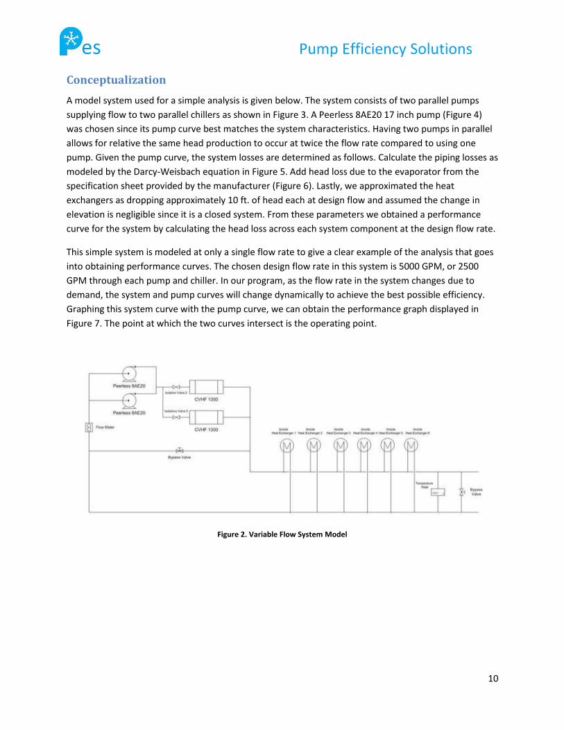
A model system used for a simple analysis is given below. The system consists of two parallel pumps
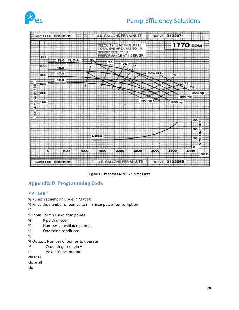
supplying flow to two parallel chillers as shown in Figure 3. A Peerless 8AE20 17 inch pump (Figure 4)
was chosen since its pump curve best matches the system characteristics. Having two pumps in parallel
allows for relative the same head production to occur at twice the flow rate compared to using one
pump. Given the pump curve, the system losses are determined as follows. Calculate the piping losses as
modeled by the Darcy-Weisbach equation in Figure 5. Add head loss due to the evaporator from the
specification sheet provided by the manufacturer (Figure 6). Lastly, we approximated the heat
exchangers as dropping approximately 10 ft. of head each at design flow and assumed the change in
elevation is negligible since it is a closed system. From these parameters we obtained a performance
curve for the system by calculating the head loss across each system component at the design flow rate.
This simple system is modeled at only a single flow rate to give a clear example of the analysis that goes
into obtaining performance curves. The chosen design flow rate in this system is 5000 GPM, or 2500
GPM through each pump and chiller. In our program, as the flow rate in the system changes due to
demand, the system and pump curves will change dynamically to achieve the best possible efficiency.
Graphing this system curve with the pump curve, we can obtain the performance graph displayed in
Figure 7. The point at which the two curves intersect is the operating point.
Figure 2. Variable Flow System Model
es Pump Efficiency Solutions
11
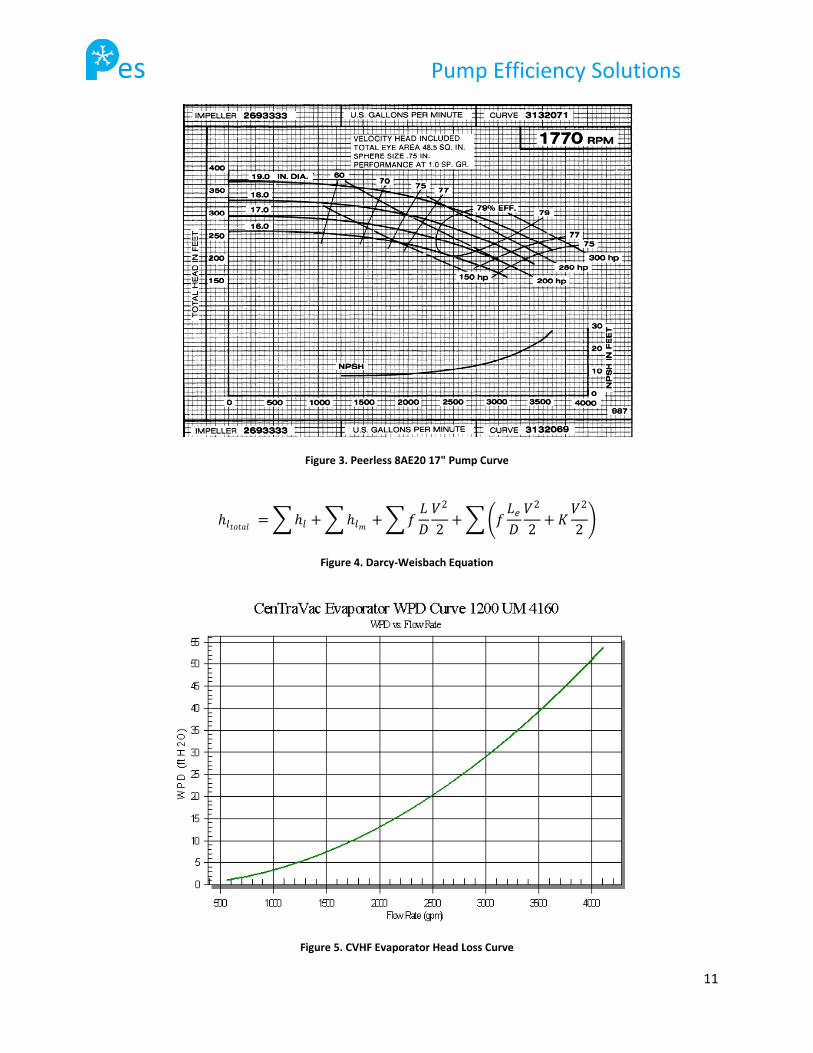
Figure 3. Peerless 8AE20 17" Pump Curve
ℎ𝑙𝑡𝑜𝑡𝑎𝑙 = ℎ𝑙 + ℎ𝑙𝑚 + 𝑓𝐿
𝐷
𝑉2
2+ 𝑓
𝐿𝑒𝐷
𝑉2
2+ 𝐾
𝑉2
2
Figure 4. Darcy-Weisbach Equation
Figure 5. CVHF Evaporator Head Loss Curve
es Pump Efficiency Solutions
12
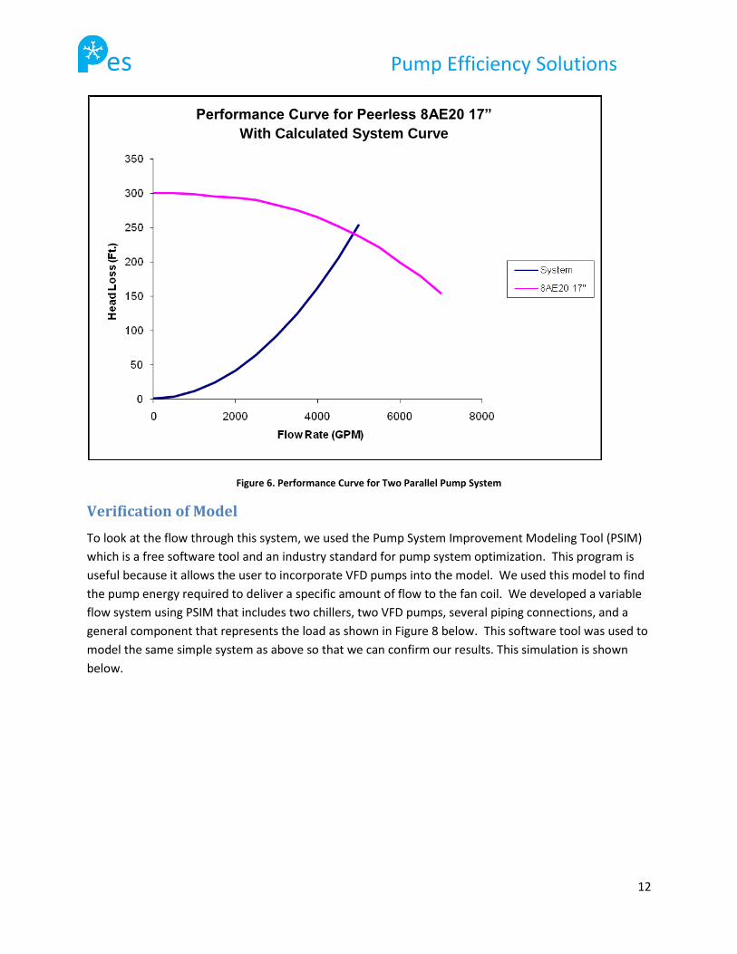
Figure 6. Performance Curve for Two Parallel Pump System
Verification of Model
To look at the flow through this system, we used the Pump System Improvement Modeling Tool (PSIM)
which is a free software tool and an industry standard for pump system optimization. This program is
useful because it allows the user to incorporate VFD pumps into the model. We used this model to find
the pump energy required to deliver a specific amount of flow to the fan coil. We developed a variable
flow system using PSIM that includes two chillers, two VFD pumps, several piping connections, and a
general component that represents the load as shown in Figure 8 below. This software tool was used to
model the same simple system as above so that we can confirm our results. This simulation is shown
below.
Performance Curve for Peerless 8AE20 17”
With Calculated System Curve
es Pump Efficiency Solutions
13
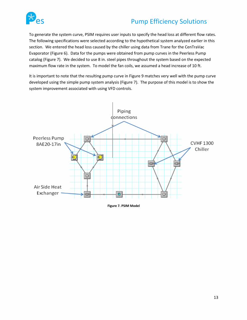
To generate the system curve, PSIM requires user inputs to specify the head loss at different flow rates.
The following specifications were selected according to the hypothetical system analyzed earlier in this
section. We entered the head loss caused by the chiller using data from Trane for the CenTraVac
Evaporator (Figure 6). Data for the pumps were obtained from pump curves in the Peerless Pump
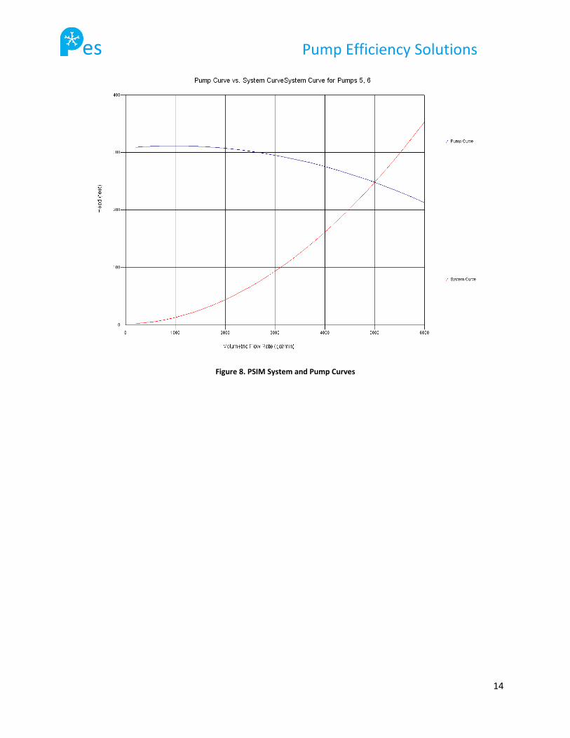
catalog (Figure 7). We decided to use 8 in. steel pipes throughout the system based on the expected
maximum flow rate in the system. To model the fan coils, we assumed a head increase of 10 ft.
It is important to note that the resulting pump curve in Figure 9 matches very well with the pump curve
developed using the simple pump system analysis (Figure 7). The purpose of this model is to show the
system improvement associated with using VFD controls.
Figure 7. PSIM Model
es Pump Efficiency Solutions
14
Figure 8. PSIM System and Pump Curves
es Pump Efficiency Solutions
15
Design Development
In creating our final product, we combined knowledge gained during modeling with fundamental
principles from Fluid Mechanics. In this segment, we created a simple analysis in Microsoft Excel.
Program Overview
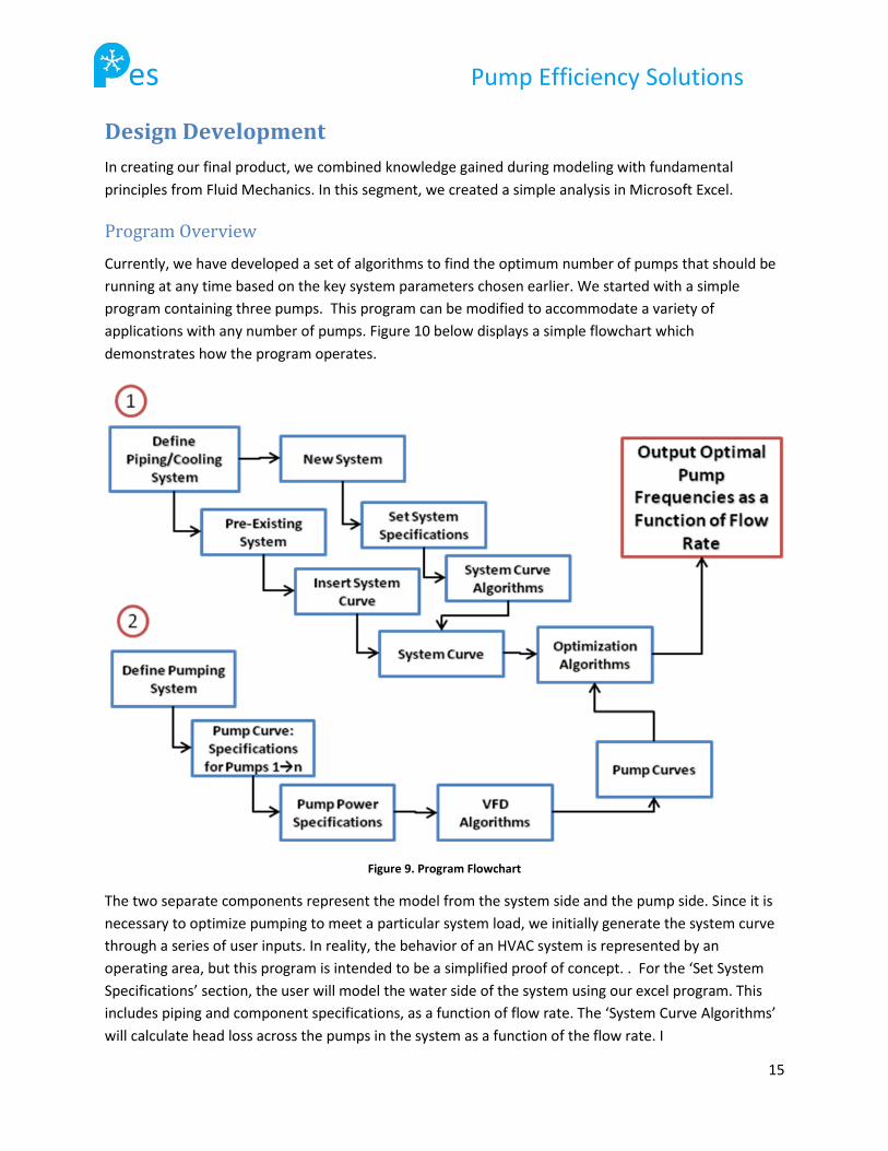
Currently, we have developed a set of algorithms to find the optimum number of pumps that should be
running at any time based on the key system parameters chosen earlier. We started with a simple
program containing three pumps. This program can be modified to accommodate a variety of
applications with any number of pumps. Figure 10 below displays a simple flowchart which
demonstrates how the program operates.
Figure 9. Program Flowchart
The two separate components represent the model from the system side and the pump side. Since it is
necessary to optimize pumping to meet a particular system load, we initially generate the system curve
through a series of user inputs. In reality, the behavior of an HVAC system is represented by an
operating area, but this program is intended to be a simplified proof of concept. . For the ‘Set System
Specifications’ section, the user will model the water side of the system using our excel program. This
includes piping and component specifications, as a function of flow rate. The ‘System Curve Algorithms’
will calculate head loss across the pumps in the system as a function of the flow rate. I
es Pump Efficiency Solutions
16
Generating the second curve involves modeling the pumping portion of the system. When the user
‘Defines the Pumping System’ they will input the number of pumps and the manner in which they are
connected (Series or Parallel). They will then be prompted to insert the ‘Pump Curve Specifications’ for
each individual pump. The pump curve provided by the manufacturer shows the head generated as a
function of flow-rate at the nominal frequency of 60Hz. The user must also input the ‘Pump Power
Specifications’ from the manufacturer. The ‘VFD Algorithms’ will then develop a series of pump curves
for frequencies from 30Hz-60Hz for each pump which plot head vs. flow rate in addition to the power
consumed and efficiency for each point.
The ‘Optimization Algorithms’ then combine the pump curves and system curves. The algorithms solve
for the most efficient operating frequency for each pump in order to match a load required by the
system on the system curve. The final result is the number of pumps, and running frequency that
provides the least power consumption as a function of system load (flow-rate).
In contrast to other pumping systems, closed circulation systems must only overcome losses due to
friction. Since the pump constantly drives water through the system, elevation changes are not an issue.
The system’s losses relate directly to the flow rate in the system. For flow through pipe sections, losses
due to friction depend on the pipe geometry, fluid properties, and flow regime. Our pipe losses were
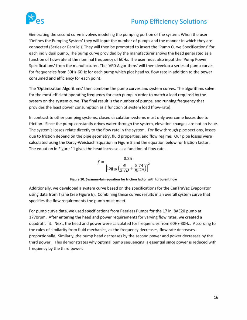
calculated using the Darcy-Weisbach Equation in Figure 5 and the equation below for friction factor.
The equation in Figure 11 gives the head increase as a function of flow rate.
𝑓 =0.25
log10 ∈
3.7𝐷+
5.74𝑅𝑒0.9
2
Figure 10. Swamee-Jain equation for friction factor with turbulent flow
Additionally, we developed a system curve based on the specifications for the CenTraVac Evaporator
using data from Trane (See Figure 6). Combining these curves results in an overall system curve that
specifies the flow requirements the pump must meet.
For pump curve data, we used specifications from Peerless Pumps for the 17 in. 8AE20 pump at
1770rpm. After entering the head and power requirements for varying flow rates, we created a
quadratic fit. Next, the head and power were calculated for frequencies from 60Hz-30Hz. According to
the rules of similarity from fluid mechanics, as the frequency decreases, flow rate decreases
proportionally. Similarly, the pump head decreases by the second power and power decreases by the
third power. This demonstrates why optimal pump sequencing is essential since power is reduced with
frequency by the third power.
es Pump Efficiency Solutions
17
The efficiency for each operating point was calculated using the following equation where Q is flow rate
in GPM, head is in feet, and Pin is in HP.
𝜂 =
𝑄𝐻3960𝑃𝑖𝑛
Figure 11. Pump efficiency equation
Sample Analysis
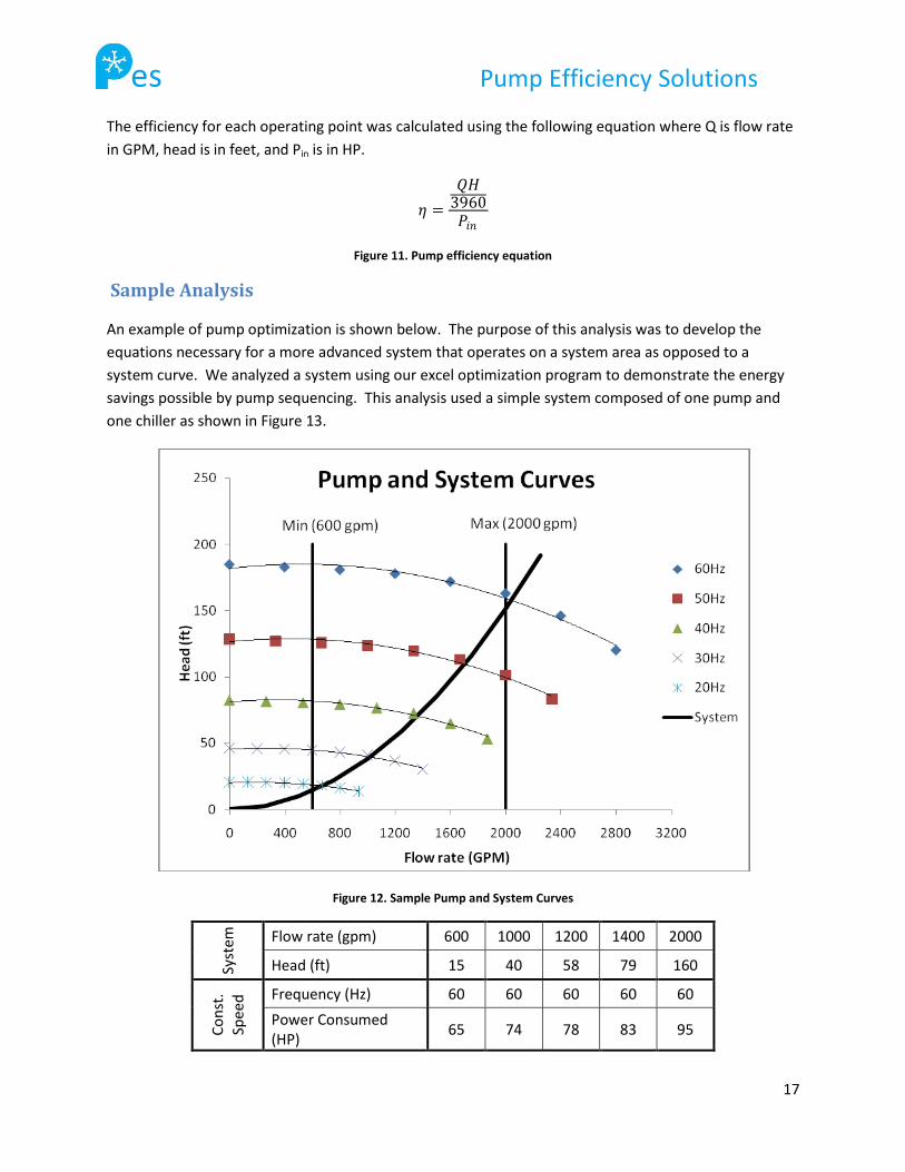
An example of pump optimization is shown below. The purpose of this analysis was to develop the
equations necessary for a more advanced system that operates on a system area as opposed to a
system curve. We analyzed a system using our excel optimization program to demonstrate the energy
savings possible by pump sequencing. This analysis used a simple system composed of one pump and
one chiller as shown in Figure 13.
Figure 12. Sample Pump and System Curves
Syst
em
Flow rate (gpm) 600 1000 1200 1400 2000
Head (ft) 15 40 58 79 160
Co
nst
. Sp
eed
Frequency (Hz) 60 60 60 60 60
Power Consumed (HP)
65 74 78 83 95
es Pump Efficiency Solutions
18
VFD
Frequency (Hz) 20 30 40 50 60
Power Consumed (HP)
4 12 27 53 95
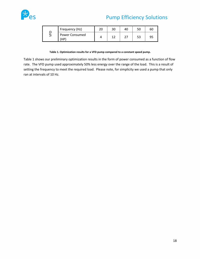
Table 1. Optimization results for a VFD pump compared to a constant speed pump.
Table 1 shows our preliminary optimization results in the form of power consumed as a function of flow
rate. The VFD pump used approximately 50% less energy over the range of the load. This is a result of
setting the frequency to meet the required load. Please note, for simplicity we used a pump that only
ran at intervals of 10 Hz.
es Pump Efficiency Solutions
19
Final Design
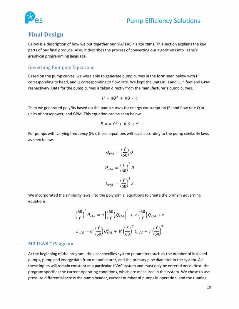
Below is a description of how we put together our MATLAB™ algorithms. This section explains the key
parts of our final produce. Also, it describes the process of converting our algorithms into Trane’s
graphical programming language.
Governing Pumping Equations
Based on the pump curves, we were able to generate pump curves in the form seen below with H
corresponding to head, and Q corresponding to flow rate. We kept the units in H and Q in feet and GPM
respectively. Data for the pump curves is taken directly from the manufacturer’s pump curves.
𝐻 = 𝑎𝑄2 + 𝑏𝑄 + 𝑐
Then we generated polyfits based on the pump curves for energy consumption (E) and flow rate Q in
units of horsepower, and GPM. This equation can be seen below.
𝐸 = 𝑎′𝑄2 + 𝑏′𝑄 + 𝑐′
For pumps with varying frequency (Hz), these equations will scale according to the pump similarity laws
as seen below.
𝑄𝑣𝑓𝑑 = 𝑓
60 𝑄
𝐻𝑣𝑓𝑑 = 𝑓
60
2
𝐻
𝐸𝑣𝑓𝑑 = 𝑓
60
3
𝐸
We incorporated the similarity laws into the polynomial equations to create the primary governing
equations.
60
𝑓
2
𝐻𝑣𝑓𝑑 = 𝑎 60
𝑓 𝑄𝑣𝑓𝑑
2
+ 𝑏 60
𝑓 𝑄𝑣𝑓𝑑 + 𝑐
𝐸𝑣𝑓𝑑 = 𝑎′ 𝑓
60 𝑄𝑣𝑓𝑑
2 + 𝑏′ 𝑓
60
2
𝑄𝑣𝑓𝑑 + 𝑐′ 𝑓
60
3
MATLAB™ Program
At the beginning of the program, the user specifies system parameters such as the number of installed
pumps, pump and energy data from manufacturer, and the primary pipe diameter in the system. All
these inputs will remain constant at a particular HVAC system and must only be entered once. Next, the
program specifies the current operating conditions, which are measured in the system. We chose to use
pressure differential across the pump header, current number of pumps in operation, and the running
es Pump Efficiency Solutions
20
frequency of these pumps as transient inputs. Each of these inputs can be measured inexpensively and
reliably, which were the main deciding factors for selecting them. We determined measuring the
system’s flow rate was too unreliable to base our algorithms on this parameter. Instead, we back
calculated the flow rate using the governing equations given above. In our code, the flow rate is
calculated twice. The first time uses the pressure difference across the header while the second
equation uses the change in pressure directly across each pump. The only difference between these
calculations is the inclusion of minor losses between the header and each pump.
In the next part, we investigated every possible pumping sequence. The program assumes that all
pumps are the same model and all operate at the same frequency, which ensures that the all pumps are
as low as possible on the energy curve. We established limits on frequency and flow rate to avoid
unattainable values. In our case, the options were running one pump, running two pumps, or running
three pumps, but this will vary for different systems since the number of options equals the number of
pumps available. For each possible case, we calculated the frequency and pumping power required to
meet the current load. Comparing these results, we identified the option with lowest energy
consumption.
MATLAB™ To Trane Graphical Programming (TGP)
The final goal of our project was to implement our algorithms within one of Trane’s controllers. In order
to implement our MATLAB™ code on Trane’s MP580 controller, we had to translate the code we had
written to Trane’s proprietary software. Trane’s software is a simple, logical, language that does not
have the capability to perform many of the operations common to more in depth programming
languages like MATLAB™. Because of this, we made some adaptations to allow our algorithms to be
implemented on the controller. An illustration of the challenges faced in the transition is shown by the
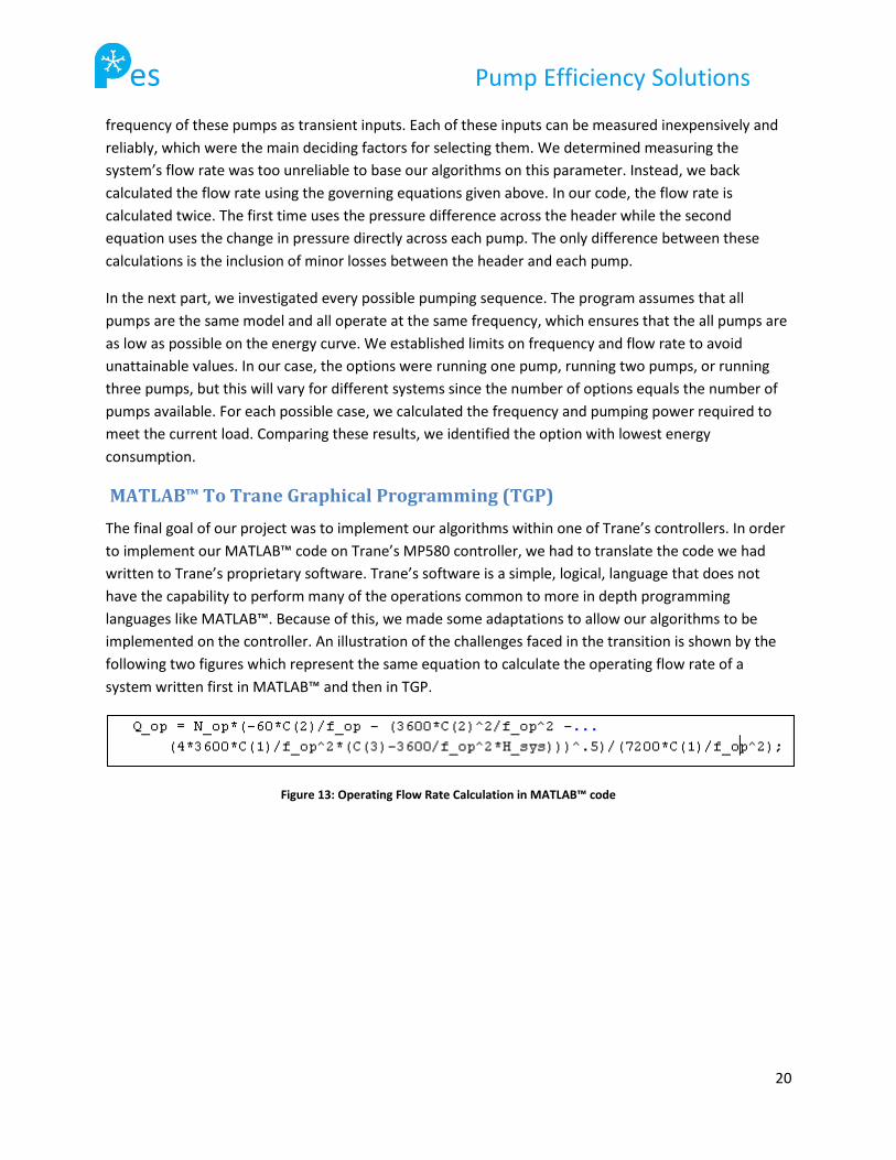
following two figures which represent the same equation to calculate the operating flow rate of a
system written first in MATLAB™ and then in TGP.
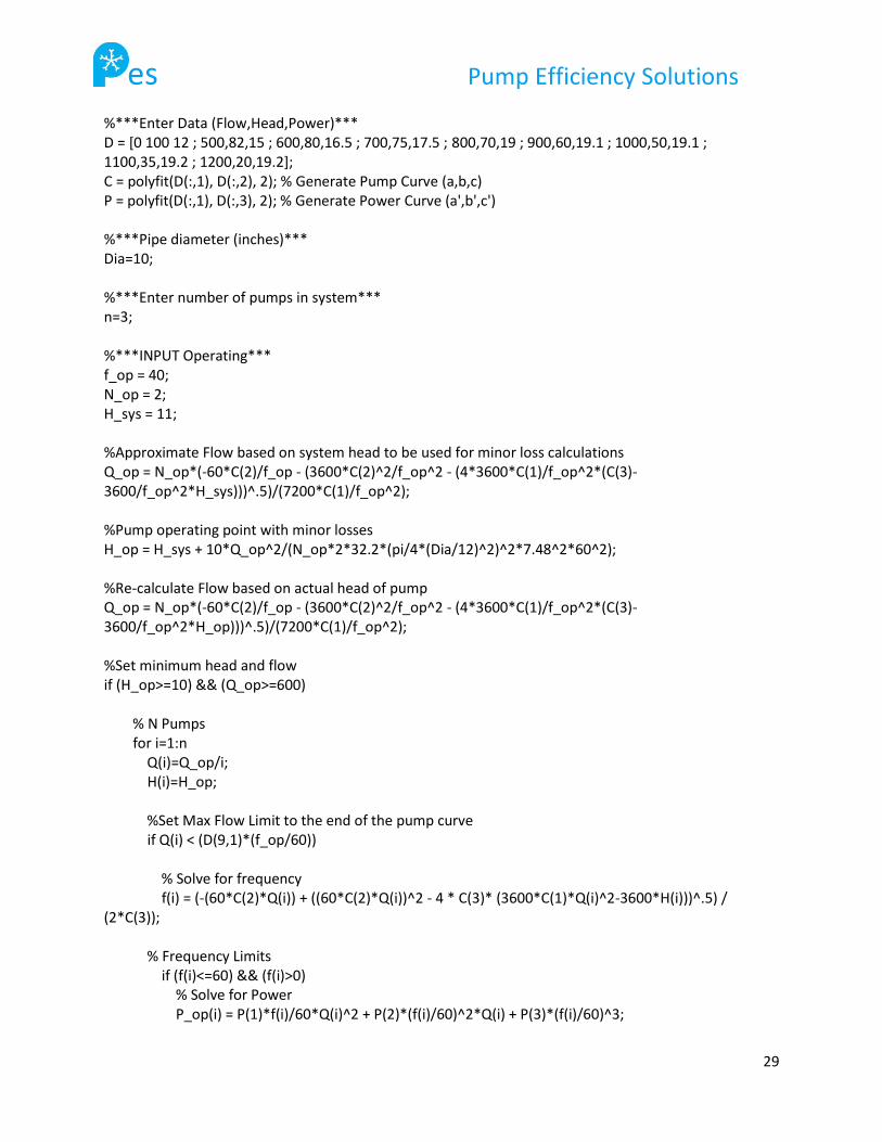
Figure 13: Operating Flow Rate Calculation in MATLAB™ code
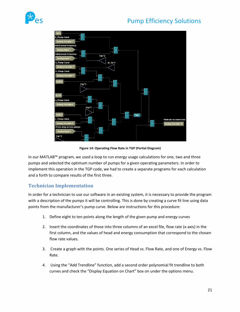
es Pump Efficiency Solutions
21
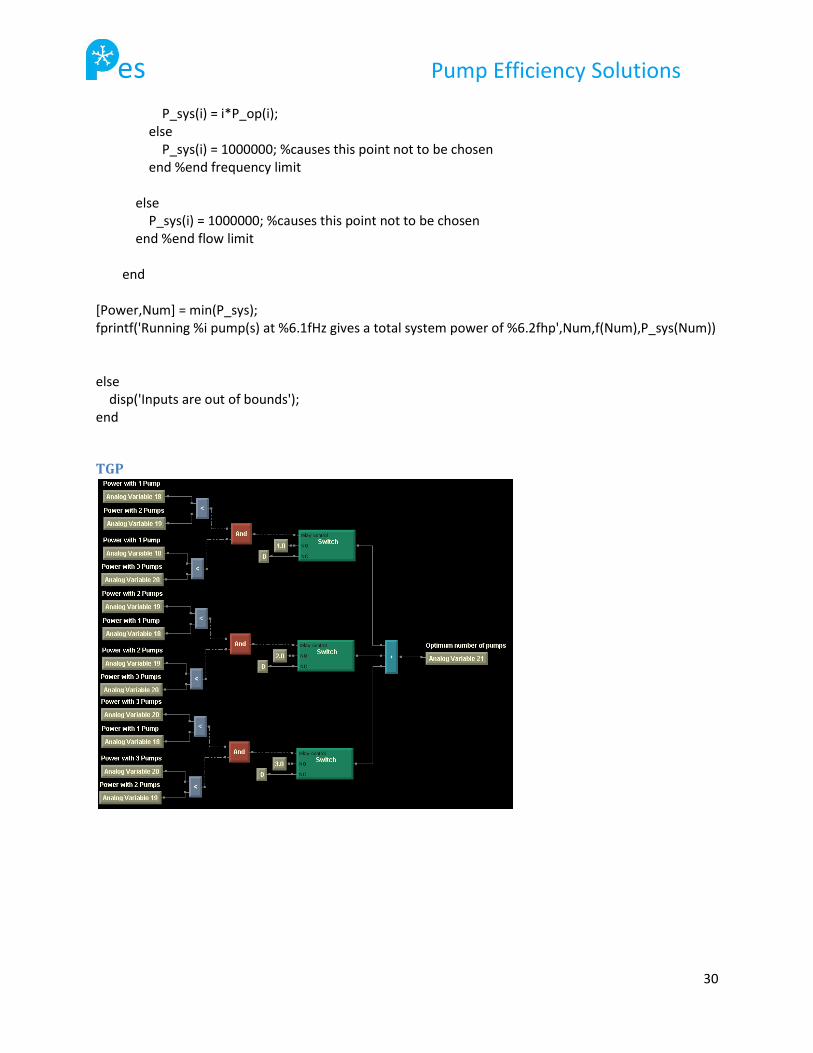
Figure 14: Operating Flow Rate in TGP (Partial Diagram)
In our MATLAB™ program, we used a loop to run energy usage calculations for one, two and three
pumps and selected the optimum number of pumps for a given operating parameters. In order to
implement this operation in the TGP code, we had to create a separate programs for each calculation
and a forth to compare results of the first three.
Technician Implementation
In order for a technician to use our software in an existing system, it is necessary to provide the program
with a description of the pumps it will be controlling. This is done by creating a curve fit line using data
points from the manufacturer’s pump curve. Below are instructions for this procedure:
1. Define eight to ten points along the length of the given pump and energy curves
2. Insert the coordinates of those into three columns of an excel file, flow rate (x-axis) in the
first column, and the values of head and energy consumption that correspond to the chosen
flow rate values.
3. Create a graph with the points. One series of Head vs. Flow Rate, and one of Energy vs. Flow
Rate.
4. Using the “Add Trendline” function, add a second order polynomial fit trendline to both
curves and check the “Display Equation on Chart” box on under the options menu.
es Pump Efficiency Solutions
22
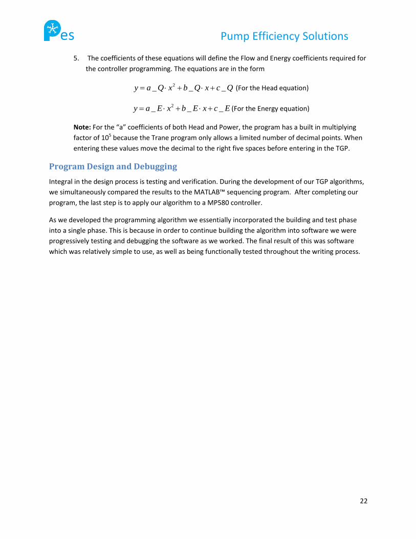
5. The coefficients of these equations will define the Flow and Energy coefficients required for
the controller programming. The equations are in the form
QcxQbxQay ___ 2 (For the Head equation)
EcxEbxEay ___ 2 (For the Energy equation)
Note: For the “a” coefficients of both Head and Power, the program has a built in multiplying
factor of 105 because the Trane program only allows a limited number of decimal points. When
entering these values move the decimal to the right five spaces before entering in the TGP.
Program Design and Debugging
Integral in the design process is testing and verification. During the development of our TGP algorithms,
we simultaneously compared the results to the MATLAB™ sequencing program. After completing our
program, the last step is to apply our algorithm to a MP580 controller.
As we developed the programming algorithm we essentially incorporated the building and test phase
into a single phase. This is because in order to continue building the algorithm into software we were
progressively testing and debugging the software as we worked. The final result of this was software
which was relatively simple to use, as well as being functionally tested throughout the writing process.
es Pump Efficiency Solutions
23
Conclusions
Using a variable frequency drive in an industrial HVAC system with proper pump sequencing provides
significant energy savings. This procedure involves varying the number of pumps running in a system, as
well as the frequency to dynamically optimize the energy usage as the cooling load increases or
decreases. We first developed models using PSIM and Excel to demonstrate the potential savings
associated with pump sequencing and to help develop the necessary algorithms. Our end goal was to
develop a non-specific program that can calculate the optimum number of pumps that should be
running for any given system characteristics. We completed this task in both MATLAB™ and Trane’s
graphical programming language. This program uses pump and energy curves, as shown in our
implementation section, and is infinitely adjustable by changing the input frequencies to the motors. As
the system pressure and flow rate requirements change, the program calculates the optimum frequency
and number of pumps to be running in the system. The challenge of the program’s algorithms was to
control this pump sequencing in such a way as to maintain the lowest energy consumption as possible.
To optimize the energy efficiency of the entire system, chiller and air-side considerations need to be
included. Our project defines the optimal pump sequencing based on flow rate requirements. Since
pumps expend approximately 40% of the system’s energy, addressing pump sequencing will have the
greatest effect on overall efficiency. A follow up project would be to create an algorithm for sequencing
chillers and incorporate heat transfer of the system though it would have a lesser effect on system
efficiency.
Another important follow up is field testing of the algorithms. The algorithms work on a theoretical
level, but we were unable to implement them into an actual control sequence for a large scale pumping
system. To be completely certain of their effectiveness, it is critical to actually test the algorithms in the
field and determine how effective they are.
The algorithms developed are capable of controlling up to three pumps in a HVAC system. With these
algorithms, we hope that Trane will be able to achieve large gains in efficiency of their systems. This
gives them an advantage in the HVAC industry as no standard currently exists for the sequencing of
variable frequency pumps.
As Trane further develops their graphical programming language, these algorithms should become more
useful. With the current version of TGP, the simple algorithms become overly complicated due to
program limitations, but as Trane further develops the software the algorithms can be integrated more
completely. Overall, the project was a great success, and we accomplished our goals of defining a
general set of pump sequencing algorithms. These algorithms can be used for many systems with VFD
pumps in parallel configurations and can optimize the sequencing of these pumps for maximum energy
efficiency.
es Pump Efficiency Solutions
24
References
"Chapter 1: Buildings Sector." Buildings Energy Data Book. U.S. Department of Energy. 16 Apr. 2009
<http://btscoredatabook.eren.doe.gov/ChapterView.aspx?chap=1>.
"Chilled water Tips. Cooling systems based on chilled water. chillers." Nanomagnetics.org -- Estudies
about the Magnetic Materials. 4 Mar. 2009 <http://www.nanomagnetics.org/chilledwatertips/>
Evans, PhD, Joe. "Understanding Pumps, Motors, and Their Controls." Pump Ed 101. 14 Jan. 2009
<http://pumped101.com/>
Fox, Robert W., Alan T. McDonald, and Philip J. Pritchard. Introduction to Fluid Mechanics. 6th ed.
Hoboken, NJ: John Wiley & Sons Inc., 2003.
Hodgson, Judy, and Trey Walters. Optimizing Pumping Systems. Tech. Woodland Park, CO: Applied Flow
Technology Corp., 1997.
PSIM. Computer software. Vers. 1. Pump Systems Matter. 28 Jan. 2007. 1 Mar. 2009
<http://pumpsystemsmatter.org/>.
Rishel, James B., Thomas H. Durkin, and Ben L. Kincaid. HVAC Pump Handbook, Second Edition
(McGraw-Hill Handbooks). 2nd ed. New York: McGraw-Hill Professional, 2006.
Schwedler, Mick. "Variable-Primary-Flow Systems Revisited." Trane Engineers Newsletter 31 (2002)
" Trane Commercial." Trane Commercial & Residential Air Solutions. 3 Feb. 2009
<http://www.trane.com/Commercial/>.
es Pump Efficiency Solutions
25
Appendices
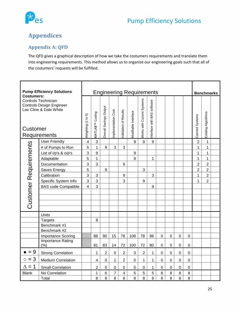
Appendix A: QFD
The QFD gives a graphical description of how we take the costumers requirements and translate them
into engineering requirements. This method allows us to organize our engineering goals such that all of
the costumers’ requests will be fulfilled.
Pump Efficiency Solutions Costumers: Controls Technician Controls Design Engineer Lee Cline & Dale White
Customer Requirements
Engineering Requirements Benchmarks
Weig
htin
g (
1 to 5
)
MA
TLA
B™
Codin
g
Overa
ll S
avin
gs O
utp
ut
Imp
lem
enta
tio
n C
ost
Valid
atio
n o
f R
esults
Mo
difia
ble
Inte
rface
Work
s w
ith C
urr
ent
Syste
ms
Inte
rface w
ith B
AS
softw
are
Canned S
yste
ms
Exis
tin
g A
lgorith
ms
Custo
mer
Re
quir
em
ents
User Friendly 4 3 9 9 9 2 1
# of Pumps to Run 5 1 9 3 3 1 1
List of i/p's & o/p's 3 9 9 1 1
Adaptable 5 1 9 1 1 1
Documentation 3 3 9 2 2
Saves Energy 5 9 3 2 2
Calibration 3 3 9 3 1 2
Specific System Info 3 3 3 9 1 2
BAS code Compatible 4 3 9
Units
Targets 8
Benchmark #1
Benchmark #2
Importance Scoring 88 90 15 78 108 78 86 0 0 0 0
Importance Rating (%) 81 83 14 72 100 72 80 0 0 0 0
● = 9 Strong Correlation 1 2 0 2 3 2 1 0 0 0 0
○ = 3 Medium Correlation 4 0 1 2 0 1 1 0 0 0 0
∆ = 1 Small Correlation 2 0 0 0 0 0 1 0 0 0 0
Blank No Correlation 1 6 7 4 5 5 5 8 8 8 8
Total 8 8 8 8 8 8 8 8 8 8 8

es Pump Efficiency Solutions
26
Table 2-QFD (House of Quality)
Appendix B: List of Vendors
Trane Commercial – Provided chiller specifications which we modeled (UVHF1300 Chiller)
Peerless Pumps – Provided pump specifications which we modeled (8AE20 17”Pump)
Pump Systems Matter – Provided PSIM software which we used for modeling.
es Pump Efficiency Solutions
27
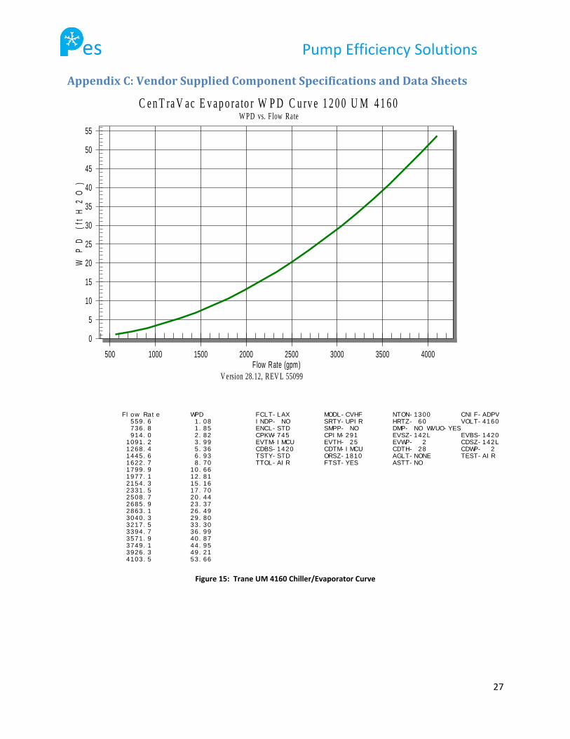
Appendix C: Vendor Supplied Component Specifications and Data Sheets
Figure 15: Trane UM 4160 Chiller/Evaporator Curve
0
5
10
15
20
25
30
35
40
45
50
55
500 1000 1500 2000 2500 3000 3500 4000
C e n T ra V a c E v a p o ra to r W P D C u rv e 1 2 0 0 U M 4 1 6 0W PD vs. Flow Rate
V ersion 28.12, REV L 55099
WP
D (
ft H
2O
)
F low Rate (gpm)
Fl ow Rat e WPD 559. 6 1 . 08 736. 8 1 . 85 914. 0 2 . 82 1091. 2 3 . 99 1268. 4 5 . 36 1445. 6 6 . 93 1622. 7 8 . 70 1799. 9 10. 66 1977. 1 12. 81 2154. 3 15. 16 2331. 5 17. 70 2508. 7 20. 44 2685. 9 23. 37 2863. 1 26. 49 3040. 3 29. 80 3217. 5 33. 30 3394. 7 36. 99 3571. 9 40. 87 3749. 1 44. 95 3926. 3 49. 21 4103. 5 53. 66
FCLT- LAX MODL- CVHF NTON- 1300 CNI F- ADPVI NDP- NO SRTY- UPI R HRTZ- 60 VOLT- 4160ENCL- STD SMPP- NO DMP- NO WVUO- YESCPKW- 745 CPI M- 291 EVSZ- 142L EVBS- 1420EVTM- I MCU EVTH- 25 EVWP- 2 CDSZ- 142LCDBS- 1420 CDTM- I MCU CDTH- 28 CDWP- 2TSTY- STD ORSZ- 1810 AGLT- NONE TEST- AI RTTOL- AI R FTST- YES ASTT- NO
es Pump Efficiency Solutions
28
Figure 16. Peerless 8AE20 17" Pump Curve
Appendix D: Programming Code
MATLAB™
% Pump Sequencing Code in Matlab % Finds the number of pumps to minimize power consumption % % Input: Pump curve data points % Pipe Diameter % Number of available pumps % Operating conditions % % Output: Number of pumps to operate % Operating frequency % Power Consumption clear all close all clc
es Pump Efficiency Solutions
29
%***Enter Data (Flow,Head,Power)*** D = [0 100 12 ; 500,82,15 ; 600,80,16.5 ; 700,75,17.5 ; 800,70,19 ; 900,60,19.1 ; 1000,50,19.1 ; 1100,35,19.2 ; 1200,20,19.2]; C = polyfit(D(:,1), D(:,2), 2); % Generate Pump Curve (a,b,c) P = polyfit(D(:,1), D(:,3), 2); % Generate Power Curve (a',b',c') %***Pipe diameter (inches)*** Dia=10; %***Enter number of pumps in system*** n=3; %***INPUT Operating*** f_op = 40; N_op = 2; H_sys = 11; %Approximate Flow based on system head to be used for minor loss calculations Q_op = N_op*(-60*C(2)/f_op - (3600*C(2)^2/f_op^2 - (4*3600*C(1)/f_op^2*(C(3)-3600/f_op^2*H_sys)))^.5)/(7200*C(1)/f_op^2); %Pump operating point with minor losses H_op = H_sys + 10*Q_op^2/(N_op*2*32.2*(pi/4*(Dia/12)^2)^2*7.48^2*60^2); %Re-calculate Flow based on actual head of pump Q_op = N_op*(-60*C(2)/f_op - (3600*C(2)^2/f_op^2 - (4*3600*C(1)/f_op^2*(C(3)-3600/f_op^2*H_op)))^.5)/(7200*C(1)/f_op^2); %Set minimum head and flow if (H_op>=10) && (Q_op>=600) % N Pumps for i=1:n Q(i)=Q_op/i; H(i)=H_op; %Set Max Flow Limit to the end of the pump curve if Q(i) < (D(9,1)*(f_op/60)) % Solve for frequency f(i) = (-(60*C(2)*Q(i)) + ((60*C(2)*Q(i))^2 - 4 * C(3)* (3600*C(1)*Q(i)^2-3600*H(i)))^.5) / (2*C(3)); % Frequency Limits if (f(i)<=60) && (f(i)>0) % Solve for Power P_op(i) = P(1)*f(i)/60*Q(i)^2 + P(2)*(f(i)/60)^2*Q(i) + P(3)*(f(i)/60)^3;
es Pump Efficiency Solutions
30
P_sys(i) = i*P_op(i); else P_sys(i) = 1000000; %causes this point not to be chosen end %end frequency limit else P_sys(i) = 1000000; %causes this point not to be chosen end %end flow limit end [Power,Num] = min(P_sys); fprintf('Running %i pump(s) at %6.1fHz gives a total system power of %6.2fhp',Num,f(Num),P_sys(Num)) else disp('Inputs are out of bounds'); end
TGP
es Pump Efficiency Solutions
31
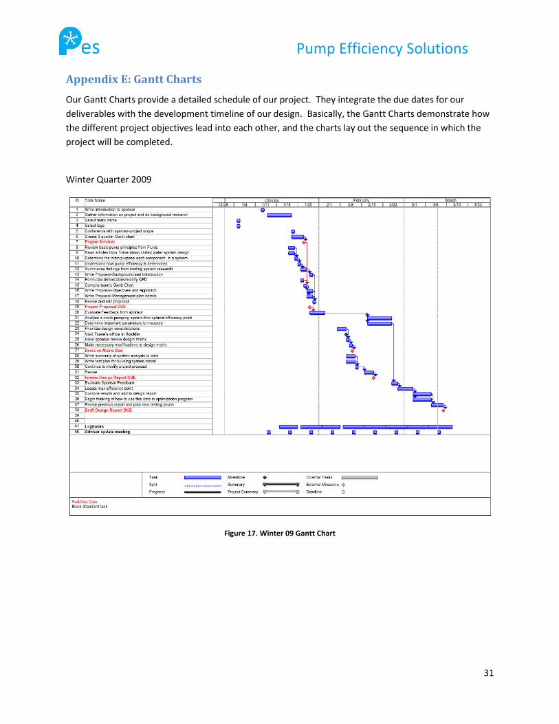
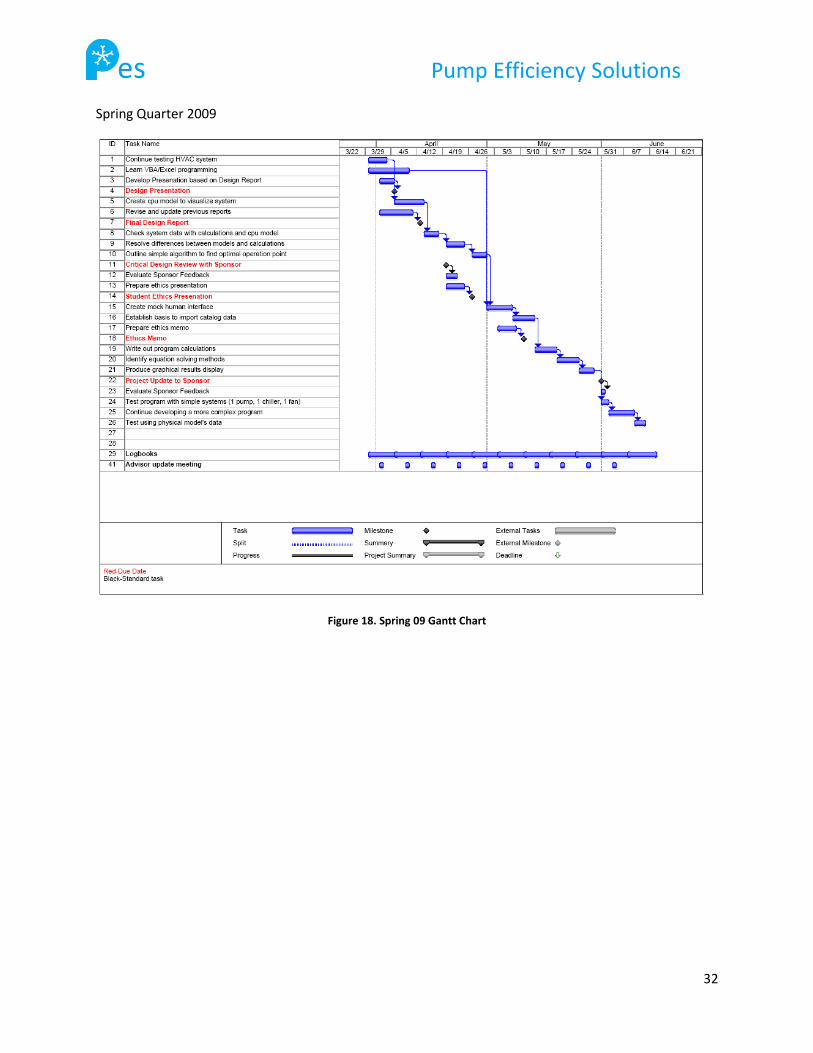
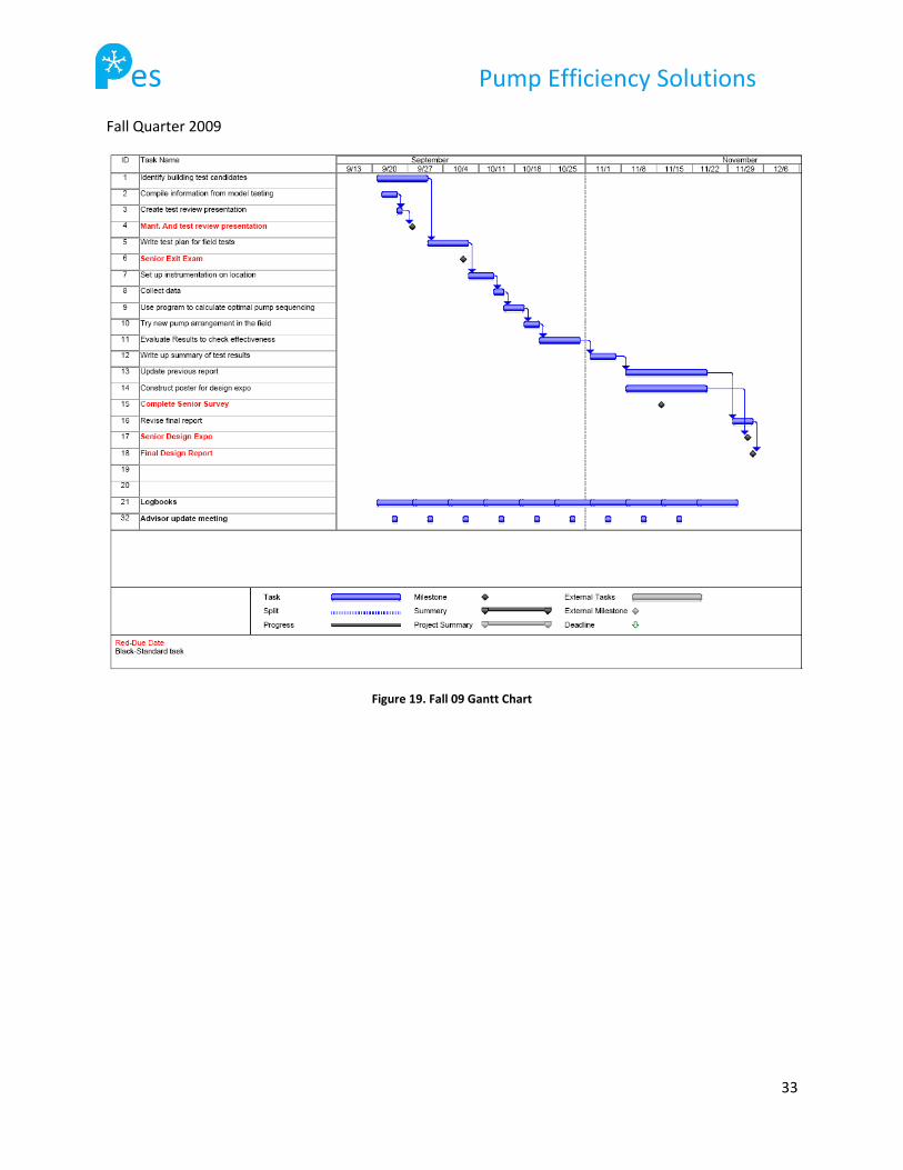
Appendix E: Gantt Charts
Our Gantt Charts provide a detailed schedule of our project. They integrate the due dates for our
deliverables with the development timeline of our design. Basically, the Gantt Charts demonstrate how
the different project objectives lead into each other, and the charts lay out the sequence in which the
project will be completed.
Winter Quarter 2009
Figure 17. Winter 09 Gantt Chart
es Pump Efficiency Solutions
32
Spring Quarter 2009
Figure 18. Spring 09 Gantt Chart
es Pump Efficiency Solutions
33
Fall Quarter 2009
Figure 19. Fall 09 Gantt Chart