Full Terms & Conditions of access and use can be found athttps://www.tandfonline.com/action/journalInformation?journalCode=tgrs20

GIScience & Remote Sensing

ISSN: 1548-1603 (Print) 1943-7226 (Online) Journal homepage: https://www.tandfonline.com/loi/tgrs20

Examining deforestation and agropasturedynamics along the Brazilian TransAmazonHighway using multitemporal Landsat imagery

Guiying Li, Dengsheng Lu, Emilio Moran, Miquéias Freitas Calvi, LucianoVieira Dutra & Mateus Batistella

To cite this article: Guiying Li, Dengsheng Lu, Emilio Moran, Miquéias Freitas Calvi, LucianoVieira Dutra & Mateus Batistella (2019) Examining deforestation and agropasture dynamics alongthe Brazilian TransAmazon Highway using multitemporal Landsat imagery, GIScience & RemoteSensing, 56:2, 161-183, DOI: 10.1080/15481603.2018.1497438

To link to this article: https://doi.org/10.1080/15481603.2018.1497438

Published online: 13 Jul 2018.

Submit your article to this journal

Article views: 169

View related articles

View Crossmark data

Citing articles: 1 View citing articles

Examining deforestation and agropasture dynamics along theBrazilian TransAmazon Highway using multitemporal Landsatimagery

Guiying Li a,b, Dengsheng Lu *a,b,c, Emilio Moranc, Miquéias Freitas Calvi d,Luciano Vieira Dutra e and Mateus Batistellaf

aFujian Provincial Key Laboratory for Subtropical Resources and Environment, Fujian NormalUniversity, 350007, Fuzhou, China; bSchool of Geographical Sciences, Fujian Normal University,350007, Fuzhou, China; cCenter for Global Change and Earth Observations, Michigan StateUniversity, 48823, East Lansing, MI, USA; dFaculty of Forestry, Federal University of Pará,68.372-040, Altamira, PA, Brazil; eImage Processing Division, National Institute for SpaceResearch, São Jose dos Campos, SP, 12245-010, Brazil; fEmbrapa Agricultural Informatics,Brazilian Agricultural Research Corporation (Embrapa), Brasília, Brazil

(Received 23 February 2018; accepted 2 July 2018)

This research aims to understand the difference of major land-cover change resultscaused in various time periods and to examine the impacts of human-induced factorson land-cover changes along the TransAmazon Highway region. The LandsatThematic Mapper and Operational Land Imager data from 2011, 2014, and 2017 andour previous land-cover classification results in 1991, 2000, and 2008 were used toexamine land-cover dynamics. A classification system consisting of five land-coverclasses – primary forest (PF), secondary forest (SF), agropasture (AP), urban area, andwater – were chosen. The hierarchical-based classification method was used to gen-erate land-cover classification results, and the post-classification comparison approachwas used to produce detailed “from-to” conversions for each detection period. Theemphasis was on deforestation of PF, dynamic change of SF and AP, and urbanizationover time. The impacts of human-induced factors such as population and economicconditions on urban expansion, AP expansion, and deforestation were examined. Thisresearch indicated that selection of a suitable time period was critical for effectivelydetecting land-cover changes; that is, too long time period (i.e., 9 years) cannotaccurately capture some land-cover changes such as the AP and SF in this research.Although deforestation – the conversion from PF to SF and AP – accounted for a largeproportion of land-cover changes, the changes between SF and AP became moreimportant than PF conversion, and required a short time period (i.e., 3 years here)for effectively reflecting their dynamics. Human-induced factors play important rolesin deforestation, dynamic changes between AP and SF, and urbanization.

Keywords: deforestation; secondary forest; agropasture expansion; TransAmazon;multitemporal Landsat imagery; human-induced factors

1. Introduction

Deforestation in the TransAmazon region in the eastern Amazon began in the 1970s dueto the construction of highways and rural settlements that attracted the migration ofpopulations from southern parts of Brazil (Moran 1975, 1981; Moran and Brondizio

*Corresponding author. Email: ludengsh@msu.edu

GIScience & Remote Sensing, 2019Vol. 56, No. 2, 161–183, https://doi.org/10.1080/15481603.2018.1497438

© 2018 Informa UK Limited, trading as Taylor & Francis Group

1998). Thousands of small farmers were attracted to the region with support from theBrazilian government and received parcels of 100 hectares of land, financing, technicalassistance, and other incentives to occupy the region and start agropastoral activities(Moran 1981), resulting in rapid agricultural expansion and extensive livestock farming(Walker, Moran, and Anselin 2000; Lu et al. 2013; Brazilian Government 2017). Therecent expansion of urban areas and the population growth caused by the construction oflarge infrastructure projects (e.g., Belo Monte Dam, about 50 km from Altamira) canenhance the impact of human actions on agroecosystems (Tundisi, Matsumura-Tundisi,and Tundisi 2015; Fearnside 2016; Moran 2016; Atkins 2017; Ritter et al. 2017). In thisregion, the agropastoral activities were mainly due to traditional systems of slash-and-burn agriculture and increased by expansion into new areas of forest (Walker, Moran, andAnselin 2000). Large areas of primary forests were replaced by pastures, agriculturallands, and cocoa plantations or secondary forests (Lu et al. 2013).

Deforestation has been regarded as an important factor resulting in environmentalproblems such as land degradation (Walker and Homma 1996). Many studies have beenconducted in the Brazilian Amazon to examine the deforestation, forest degradation andrestoration, as well as the agricultural and pastoral expansions (Lu et al. 2013; Spera et al.2014; Chen et al. 2015; Imbach et al. 2015; Müller, Griffiths, and Hostert 2016; Grecchiet al. 2017). Remote sensing technology has long been used for detecting deforestationbecause it can acquire data repeatedly with large coverage, especially when long-termLandsat images are available at no cost (Brondízio 2005; Schneibel et al. 2017; Shimizuet al. 2017). Therefore, much research explored the approaches to accurately detect thechanges in different land covers (Lu et al. 2004c; Grecchi et al. 2014; Lu, Li, and Moran2014; Beuchle et al. 2015; Silveira et al. 2018). Grecchi et al. (2014) conducted researchon land-use and land-cover changes and their impact on the environment in southeastMato Grosso State based on Landsat, MODIS, and elevation data using post-classificationcomparison methods, and found that during 1985–1995, crops (rice and soy bean)expanded at high rates, and a large part of Cerrado, Brazil’s tropical savanna ecoregion,was converted to agriculture. After 1995, crops continued to expand and encroached intofragile environments such as wetlands and more erodible soils. Between 1985 and 2005,approximately 42% of predominantly vegetated area was lost to agriculture, and soilerosion increased significantly. Silveira et al. (2018) developed a new method for detect-ing seasonal changes in Brazilian savannahs. This method used an object-based approachto extract geostatistical features from bitemporal Landsat Thematic Mapper (TM) images(wet and dry seasons). The results indicated that change detection accuracies have beengreatly improved by using the most geostatistical features compared with the spectralfeatures and image differencing technique.

In general, most change detection studies cover two broad categories: selection ofsuitable remote sensing parameters and use of proper algorithms. The parameters can bepixel-based, object-based (e.g., image segmentation based on high spatial resolutionimages), and subpixel-based (fractional images) (Lu, Li, and Moran 2014). The changedetection algorithm can also be separated into two broad categories: detecting the binarychange and non-change and detecting the detailed change trajectories. Most of the changedetection techniques such as principal component analysis and image differencing canonly detect change and non-change information using the thresholding-based approach(Lu et al. 2004c). However, the change and non-change information cannot providesufficient information required for particular purposes (e.g., driving forces of deforesta-tion, land-cover and land-use change modelling); detailed change trajectories are oftenneeded, for which the post-classification comparison approach is commonly used (Lu

162 G. Li et al.

et al. 2013). The post-classification comparison method involves classification of indivi-dual images into land-cover maps at multitemporal scale and comparison of classifiedland-cover maps pixel by pixel. This method provides detailed “from-to” change trajec-tories and identifies where the change occurred and how much change occurred. Theaccuracy of change detection is dependent on the accuracy of each individual classifica-tion. However, every error in the individual classification map will be carried over into thefinal change detection. Thus, caution must be taken to ensure that all individual classifica-tions are as accurate as possible.

In addition to the selection of suitable remote sensing data and algorithms, determinationof suitable time periods is an important concern for effectively obtaining the needed changeinformation. A long time period may hide the real changes, while a short time period may notcapture the changes. One objective of this research was to understand the effects of differenttime periods in reflecting change detection results; thus, we compared the spatial patterns ofdeforestation and agropasture dynamic changes at nine(or eight)-year intervals (1991–2000–2008–2017) and at three-year intervals (2008–2011–2014–2017). Another objective was toexamine the human-induced activities on these changes along the TransAmazon Highwayregion and the potential impacts of Belo Monte dam construction on deforestation andagropasture expansion in an area not directly affected by the construction but indirectlyaffected by the growth of population, loss of farm workers to dam construction, and theabsence of policies directed at the agrarian sector during this period.

2. Study area

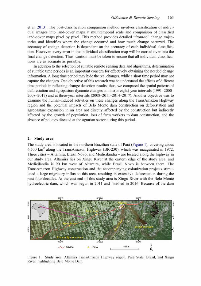
The study area is located in the northern Brazilian state of Pará (Figure 1), covering about6,500 km2 along the TransAmazon Highway (BR-230), which was inaugurated in 1972.Three cities – Altamira, Brasil Novo, and Medicilândia – are located along the highway inour study area. Altamira lies on Xingu River at the eastern edge of the study area, andMedicilândia is 90 km west of Altamira, while Brasil Novo is between them. TheTransAmazon Highway construction and the accompanying colonization projects stimu-lated a large migratory influx to this area, resulting in extensive deforestation during thepast four decades. At the east end of this study area is Xingu River with the Belo Montehydroelectric dam, which was begun in 2011 and finished in 2016. Because of the dam

Figure 1. Study area: Altamira TransAmazon Highway region, Pará State, Brazil, and XinguRiver, highlighting Belo Monte Dam.

GIScience & Remote Sensing 163

construction, large numbers of people moved to Altamira and nearby construction sites,resulting in expanded urbanization (Feng et al. 2017).

A large area of primary forests has been converted to successional vegetation, pasture,and agricultural lands since the early 1970s (Moran et al. 1994; Moran and Brondizio1998; Lu et al. 2013). Cocoa plantations and livestock are the most important economicactivities in this region. The cocoa plantations are commonly located in areas of Nitisolsand Ferralsols and cultivated under agroforestry systems, resulting in complex foreststructures in density and canopy strata (Calvi 2009). The yellow-colored Ferralsolsareas (the most abundant soils in the region) are mainly used for the cultivation ofpastures for raising cattle. Annual crops are grown at a reduced scale, usually at anearly stage or concomitant with the planting of cocoa or pasture.

The study area is characterized by moderately rolling uplands with the highestelevation of approximately 350 m. The area has tropical climate with average annualtemperature of 26ºC degrees and average annual precipitation of 2000 mm (Tucker,Brondizio, and Morán 1998). The temperature varies little throughout the year, butprecipitation has significant seasonal variation, and most precipitation occurs from lateOctober to early June.

3. Materials and methods

3.1. Data collection and preprocessing

The data used in this study are summarized in (Table 1). Multitemporal Landsat TM andOperational Land Imager images (path/row 226/62) covering 2011, 2014, and 2017were usedto develop land-cover distribution and dynamics. All Landsat images were atmosphericallycalibrated using the improved image-based dark object subtraction method (Chávez 1996;Chander, Markham, and Helder 2009) and co-registered to the Universal Transverse Mercatorcoordinate system. The root mean squared errors for the georegistration were less than 0.5pixels, ensuring their geometric accuracy for change detection. Our previous research con-ducted land-cover classification using the Landsat TM images, and the results in 1991, 2000,

Table 1. Datasets used in research.

Dataset Sources and dates

Landsat images (1) Landsat 5 TM on 27 July 2011(2) Landsat 8 OLI image on 20 August 2014(3) Landsat 8 OLI images on June 16 and 11 July 2017Spectral bands of blue, green, red, near infrared, and two short wavelength infraredfrom Landsat TM and OLI were used to develop land-cover maps

Land-coverimages

Land-cover classification results were developed from Landsat TM images in1991, 2000 and 2008 and were directly used in this research. The detaileddescriptions of these classification results are provided in Lu et al. (2013).

SPOT 6 Satellite Pour l’Observation de la Terre (SPOT 6) imagery on 19 August 2015, wasused for collection of land-cover samples.

Fieldwork Different land-cover data were collected in January–May 2015Roads The roads were digitized from Google Earth imagesPopulationGDPHerds of cattle

Data downloaded from Instituto Brasileiro de Geografia e Estatística for differentyears

Note: GDP, gross domestic product; TM, Thematic Mapper; OLI, Operational Land Imager

164 G. Li et al.

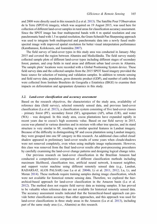
and 2008 were directly used in this research (Lu et al. 2013). The Satellite Pour l’Observationde la Terre (SPOT-6) imagery, which was acquired on 19 August 2015, was used here forcollection of different land-cover samples in rural areas for classification accuracy assessment.Since the SPOT image has four multispectral bands with 6 m spatial resolution and onepanchromatic bandwith 1.5m spatial resolution, the Gram-Schmidt Pan Sharpening approachwas used to integrate both multispectral and panchromatic data into a newly fused multi-spectral image with improved spatial resolution for better visual interpretation performance(Karathanassi, Kolokousis, and Ioannidou 2007).

The field survey of land-cover types in this study area was conducted in January–May2015 and covered the region between Altamira and Medicilândia. The field survey mainlycollected sample plots of different land-cover types including different stages of secondaryforest, pasture, and crop fields in rural areas and different urban land covers in Altamira.The sample plots’ locations were recorded with a Global Positioning System device. Thesefield survey data and the collected samples from the 2015 SPOT fused imagery provided thebasic source for selection of training and validation samples. In addition to remote sensingand field survey data, population, gross domestic product (GDP), and number of cattle herdswere collected from Instituto Brasileiro de Geografia e Estatística (IBGE) to examine theirimpacts on deforestation and agropasture dynamics in this study.

3.2. Land-cover classification and accuracy assessment

Based on the research objectives, the characteristics of the study area, availability ofreference data (field survey), selected remotely sensed data, and previous land-coverclassification (Lu et al. 2013), a classification system consisting of five land-cover classes– primary forest (PF), secondary forest (SF), agropasture (AP), urban (UR), and water(WA) – was designed. In this study area, cocoa plantations have expanded rapidly inrecent years due to cocoa’s high economic value. Based on our field survey in 2015,cocoa was planted in various densities and in mixture with other tree species, and its standstructure is very similar to SF, resulting in similar spectral features in Landsat imagery.Because of the difficulty in distinguishing SF and cocoa plantation using Landsat imagery,they were grouped into one SF category in this research. An additional class called cloud/shadow appeared in preliminary land-cover results of some years when clouds/shadowswere not removed completely, even when using multiple image replacements. However,this class was removed from the final land-cover results after post-processing proceduresby carefully examining the land-cover change patterns and designing logical change rules.

Our previous research on land-cover classification in the Brazilian Amazon hadconducted a comprehensive comparison of different classification methods includingmaximum likelihood, classification tree, artificial neural network, k-nearest neighbor,and support vector machine using different remotely sensed data (e.g., Landsat,RADARSAT, ALOS PALSAR) (see Lu et al. 2004b; Li et al. 2011, 2012; Lu, Li, andMoran 2014). These methods require training samples during image classification, whichwere not available for historical remote sensing data. Therefore, we explored the hier-archical-based approach for land-cover classification in the Amazon basin (Lu et al.2012). The method does not require field survey data as training samples. It has provedto be valuable when reference data are not available for historical remotely sensed data.The accuracy assessment results indicated that the hierarchical-based approach can pro-vide better classification accuracy than other approaches, and this approach was used forland-cover classifications in three study areas in the Amazon (Lu et al. 2013), includingpart of the same study area (i.e., Altamira) as this research.

GIScience & Remote Sensing 165

(Figure 2) illustrates the modified hierarchical classification. This method involvedstratification and cluster analysis. UR was first extracted from Landsat multispectralimages using a combination of thresholding, cluster analysis, and manual editing. Thethreshold of 0.4 based on high-albedo and low-albedo objects was used to produce theinitial UR class (Lu et al. 2010). The spectral signatures of this initial UR class wereextracted, and cluster analysis was used to classify these pixels into 30 clusters. Theanalyst merged the cluster into UR and other to improve the UR extraction accuracy.As shown in (Figure 2), UR was masked from the Landsat imagery, PF was thenextracted from Landsat multispectral images using the combination of thresholding ona normalized difference vegetation index image and cluster analysis. The same pro-cedure was used to extract WA, SF, and AP. After masking the extracted land-coverclasses from Landsat imagery, some pixels still could not be directly extracted usingthe above procedure. The remaining pixels were classified into 50 clusters usingcluster analysis. Each cluster was carefully examined with the assistance of the 2015field survey data and labeled as one of the predefined land-cover types. This hier-archical-based classification method was used for generating preliminary land-coverclassification results for 2011, 2014, and 2017.

Due to spectral similarity between land-cover classes such as UR and AP, and PFand SF, misclassification is inevitable during the classification process. Expert rulesbased on comparison of multitemporal land-cover images and logical reasoning wereused on the initial land-cover results to refine the land covers. The major rules andrefinements are listed below:

Figure 2. The modified strategy for mapping land-cover distribution from Landsat imagery usingthe hierarchical-based approach (Note: TM, Thematic Mapper; NDVI, normalized difference vege-tation index; MNDWI, modification of normalized difference water index; SF, secondary forest; AP,agropasture).

166 G. Li et al.

(1) Majority filter: Majority filter function with a window size of 3 × 3 pixels wasapplied to initial land-cover classification images of each time period to eliminateisolated pixels and reduce the salt-and-pepper problem in the classified image.

(2) Manual editing: Clouds/shadows were superimposed onto the original Landsatimage of 2014 with images from 2011 and 2017 side by side. By visual examina-tion and manual interpretation, the clouds/shadows pixels were re-assigned toappropriate land-cover classes.

(3) Automatic replacement: In reality, once PF land is cleared out, it has little or nochance to return to PF but can convert to other types of land cover; in contrast,once UR is established, it has little possibility to convert to other land-cover types.Based on these assumptions, the following automatic replacement rules werecreated: If pixels in the prior-date classification image were classified as SF, butthey were classified as PF in the posterior-date image, these pixels in the poster-ior-date image were re-assigned to SF; if pixels in the prior-date classificationimage were classified as UR but were classified as AP in the posterior-dateclassification image, these pixels were re-assigned to UR in the posterior-dateclassification image, except the buildings and roads in flooding regions.

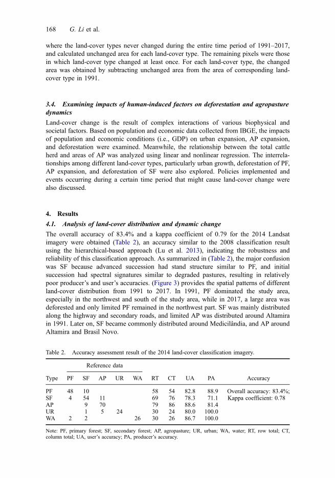
After the post-refining process on all land-cover maps of different years, the multi-temporal land-cover images were generated. Ideally, the land-cover image of every timeperiod needs to undergo accuracy assessment. However, the only available field data werecollected in 2015. Thus only the 2014 classification result was evaluated, and classifica-tions in 2011 and 2017 were not assessed due to lack of concurrent ground truth. Besidesthe sample plots collected from the field in 2015, we also collected samples from the pan-sharpened SPOT image. A total of 266 samples were used to assess the accuracy of the2014 classification. An error matrix was produced, and overall accuracy, kappa coeffi-cient, producer’s accuracy, and user’s accuracy were calculated (Foody 2002; Congaltonand Green 2009).

3.3. Analysis of land-cover dynamic changes

The area of each land-cover class at each time point was calculated based on a classifiedimage, and percentages of corresponding land covers accounting for the whole study areawere also computed. The annual land-cover change is the changed area of each land-covertype between two dates divided by the number of years within the detection period. Theseresults can provide general gains or losses of land-cover types, but they are not able toprovide detailed land-cover conversion information. Therefore, the post-classificationcomparison approach was conducted, producing a two-way conversion matrix and areasof detailed “from-to” conversions for each detection period. In particular, the emphasiswas on PF deforestation (conversion of PF to other land-cover types), dynamic change ofSF and AP (loss/gain of SF and AP), and urbanization over time.

Pairwise comparison of land covers at two dates is efficient for identifying the changesin short time periods. For longer time periods, it underestimates the extent of land-coverchange because it does not count the reversion changes occurring along the time course.For example, SF in the earliest investigation date may convert to AP at one time point,and later on, AP may change back to SF. Those changes cannot be detected andmistakenly identified as unchanged. Our field work in 2015 confirmed that some pasturelands were converted to cocoa plantations in recent years. To better reveal the extent ofland-cover change, we combined the land-cover maps of all dates and extracted the pixels

GIScience & Remote Sensing 167

where the land-cover types never changed during the entire time period of 1991–2017,and calculated unchanged area for each land-cover type. The remaining pixels were thosein which land-cover type changed at least once. For each land-cover type, the changedarea was obtained by subtracting unchanged area from the area of corresponding land-cover type in 1991.

3.4. Examining impacts of human-induced factors on deforestation and agropasturedynamics

Land-cover change is the result of complex interactions of various biophysical andsocietal factors. Based on population and economic data collected from IBGE, the impactsof population and economic conditions (i.e., GDP) on urban expansion, AP expansion,and deforestation were examined. Meanwhile, the relationship between the total cattleherd and areas of AP was analyzed using linear and nonlinear regression. The interrela-tionships among different land-cover types, particularly urban growth, deforestation of PF,AP expansion, and deforestation of SF were also explored. Policies implemented andevents occurring during a certain time period that might cause land-cover change werealso discussed.

4. Results

4.1. Analysis of land-cover distribution and dynamic change

The overall accuracy of 83.4% and a kappa coefficient of 0.79 for the 2014 Landsatimagery were obtained (Table 2), an accuracy similar to the 2008 classification resultusing the hierarchical-based approach (Lu et al. 2013), indicating the robustness andreliability of this classification approach. As summarized in (Table 2), the major confusionwas SF because advanced succession had stand structure similar to PF, and initialsuccession had spectral signatures similar to degraded pastures, resulting in relativelypoor producer’s and user’s accuracies. (Figure 3) provides the spatial patterns of differentland-cover distribution from 1991 to 2017. In 1991, PF dominated the study area,especially in the northwest and south of the study area, while in 2017, a large area wasdeforested and only limited PF remained in the northwest part. SF was mainly distributedalong the highway and secondary roads, and limited AP was distributed around Altamirain 1991. Later on, SF became commonly distributed around Medicilândia, and AP aroundAltamira and Brasil Novo.

Table 2. Accuracy assessment result of the 2014 land-cover classification imagery.

Type

Reference data

RT CT UA PA AccuracyPF SF AP UR WA

PF 48 10 58 54 82.8 88.9 Overall accuracy: 83.4%;Kappa coefficient: 0.78SF 4 54 11 69 76 78.3 71.1

AP 9 70 79 86 88.6 81.4UR 1 5 24 30 24 80.0 100.0WA 2 2 26 30 26 86.7 100.0

Note: PF, primary forest; SF, secondary forest; AP, agropasture; UR, urban; WA, water; RT, row total; CT,column total; UA, user’s accuracy; PA, producer’s accuracy.

168 G. Li et al.

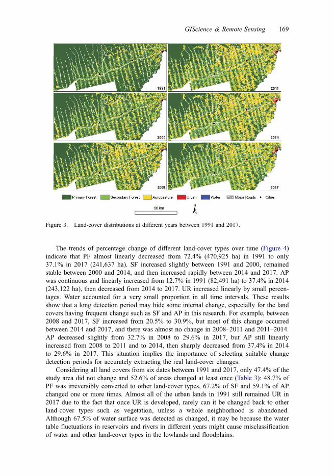
The trends of percentage change of different land-cover types over time (Figure 4)indicate that PF almost linearly decreased from 72.4% (470,925 ha) in 1991 to only37.1% in 2017 (241,637 ha). SF increased slightly between 1991 and 2000, remainedstable between 2000 and 2014, and then increased rapidly between 2014 and 2017. APwas continuous and linearly increased from 12.7% in 1991 (82,491 ha) to 37.4% in 2014(243,122 ha), then decreased from 2014 to 2017. UR increased linearly by small percen-tages. Water accounted for a very small proportion in all time intervals. These resultsshow that a long detection period may hide some internal change, especially for the landcovers having frequent change such as SF and AP in this research. For example, between2008 and 2017, SF increased from 20.5% to 30.9%, but most of this change occurredbetween 2014 and 2017, and there was almost no change in 2008–2011 and 2011–2014.AP decreased slightly from 32.7% in 2008 to 29.6% in 2017, but AP still linearlyincreased from 2008 to 2011 and to 2014, then sharply decreased from 37.4% in 2014to 29.6% in 2017. This situation implies the importance of selecting suitable changedetection periods for accurately extracting the real land-cover changes.

Considering all land covers from six dates between 1991 and 2017, only 47.4% of thestudy area did not change and 52.6% of areas changed at least once (Table 3): 48.7% ofPF was irreversibly converted to other land-cover types, 67.2% of SF and 59.1% of APchanged one or more times. Almost all of the urban lands in 1991 still remained UR in2017 due to the fact that once UR is developed, rarely can it be changed back to otherland-cover types such as vegetation, unless a whole neighborhood is abandoned.Although 67.5% of water surface was detected as changed, it may be because the watertable fluctuations in reservoirs and rivers in different years might cause misclassificationof water and other land-cover types in the lowlands and floodplains.

Figure 3. Land-cover distributions at different years between 1991 and 2017.

GIScience & Remote Sensing 169

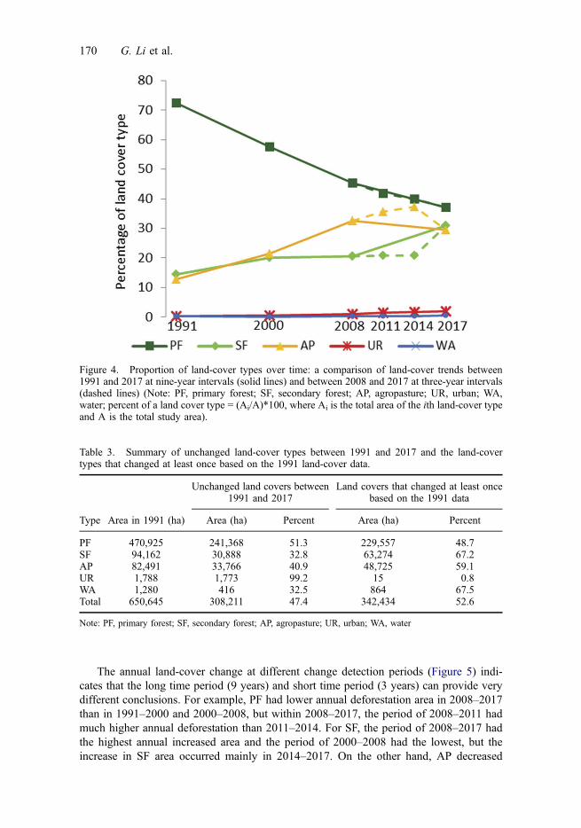
The annual land-cover change at different change detection periods (Figure 5) indi-cates that the long time period (9 years) and short time period (3 years) can provide verydifferent conclusions. For example, PF had lower annual deforestation area in 2008–2017than in 1991–2000 and 2000–2008, but within 2008–2017, the period of 2008–2011 hadmuch higher annual deforestation than 2011–2014. For SF, the period of 2008–2017 hadthe highest annual increased area and the period of 2000–2008 had the lowest, but theincrease in SF area occurred mainly in 2014–2017. On the other hand, AP decreased

Figure 4. Proportion of land-cover types over time: a comparison of land-cover trends between1991 and 2017 at nine-year intervals (solid lines) and between 2008 and 2017 at three-year intervals(dashed lines) (Note: PF, primary forest; SF, secondary forest; AP, agropasture; UR, urban; WA,water; percent of a land cover type = (Ai/A)*100, where Ai is the total area of the ith land-cover typeand A is the total study area).

Table 3. Summary of unchanged land-cover types between 1991 and 2017 and the land-covertypes that changed at least once based on the 1991 land-cover data.

Type Area in 1991 (ha)

Unchanged land covers between1991 and 2017

Land covers that changed at least oncebased on the 1991 data

Area (ha) Percent Area (ha) Percent

PF 470,925 241,368 51.3 229,557 48.7SF 94,162 30,888 32.8 63,274 67.2AP 82,491 33,766 40.9 48,725 59.1UR 1,788 1,773 99.2 15 0.8WA 1,280 416 32.5 864 67.5Total 650,645 308,211 47.4 342,434 52.6

Note: PF, primary forest; SF, secondary forest; AP, agropasture; UR, urban; WA, water

170 G. Li et al.

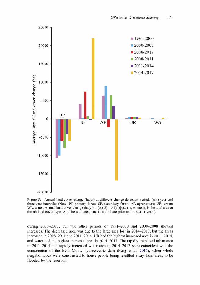
during 2008–2017, but two other periods of 1991–2000 and 2000–2008 showedincreases. The decreased area was due to the large area lost in 2014–2017, but the areasincreased in 2008–2011 and 2011–2014. UR had the highest increased area in 2011–2014,and water had the highest increased area in 2014–2017. The rapidly increased urban areain 2011–2014 and rapidly increased water area in 2014–2017 were coincident with theconstruction of the Belo Monte hydroelectric dam (Feng et al. 2017), when wholeneighborhoods were constructed to house people being resettled away from areas to beflooded by the reservoir.

Figure 5. Annual land-cover change (ha/yr) at different change detection periods (nine-year andthree-year intervals) (Note: PF, primary forest; SF, secondary forest; AP, agropasture; UR, urban;WA, water; Annual land-cover change (ha/yr) = [Ai(t2) – Ai(t1)]/(t2-t1), where Ai is the total area ofthe ith land cover type, A is the total area, and t1 and t2 are prior and posterior years).

GIScience & Remote Sensing 171

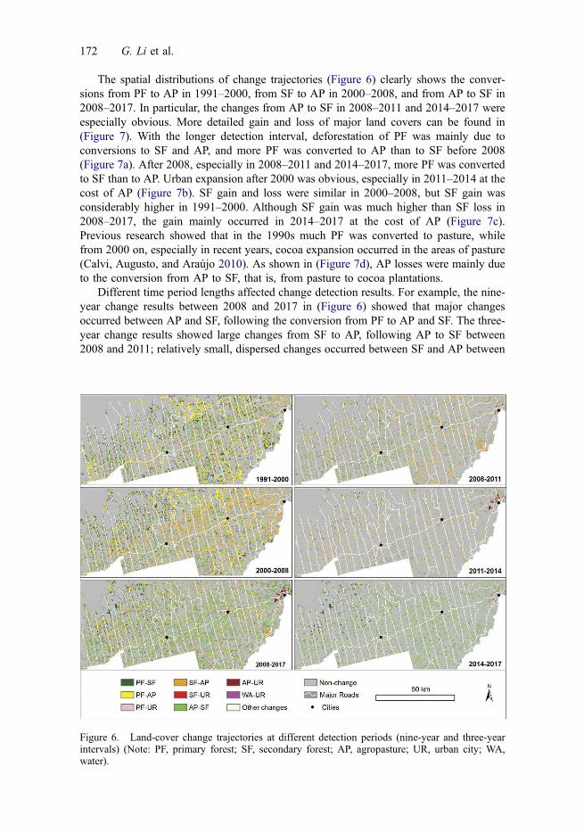
The spatial distributions of change trajectories (Figure 6) clearly shows the conver-sions from PF to AP in 1991–2000, from SF to AP in 2000–2008, and from AP to SF in2008–2017. In particular, the changes from AP to SF in 2008–2011 and 2014–2017 wereespecially obvious. More detailed gain and loss of major land covers can be found in(Figure 7). With the longer detection interval, deforestation of PF was mainly due toconversions to SF and AP, and more PF was converted to AP than to SF before 2008(Figure 7a). After 2008, especially in 2008–2011 and 2014–2017, more PF was convertedto SF than to AP. Urban expansion after 2000 was obvious, especially in 2011–2014 at thecost of AP (Figure 7b). SF gain and loss were similar in 2000–2008, but SF gain wasconsiderably higher in 1991–2000. Although SF gain was much higher than SF loss in2008–2017, the gain mainly occurred in 2014–2017 at the cost of AP (Figure 7c).Previous research showed that in the 1990s much PF was converted to pasture, whilefrom 2000 on, especially in recent years, cocoa expansion occurred in the areas of pasture(Calvi, Augusto, and Araújo 2010). As shown in (Figure 7d), AP losses were mainly dueto the conversion from AP to SF, that is, from pasture to cocoa plantations.

Different time period lengths affected change detection results. For example, the nine-year change results between 2008 and 2017 in (Figure 6) showed that major changesoccurred between AP and SF, following the conversion from PF to AP and SF. The three-year change results showed large changes from SF to AP, following AP to SF between2008 and 2011; relatively small, dispersed changes occurred between SF and AP between

Figure 6. Land-cover change trajectories at different detection periods (nine-year and three-yearintervals) (Note: PF, primary forest; SF, secondary forest; AP, agropasture; UR, urban city; WA,water).

172 G. Li et al.

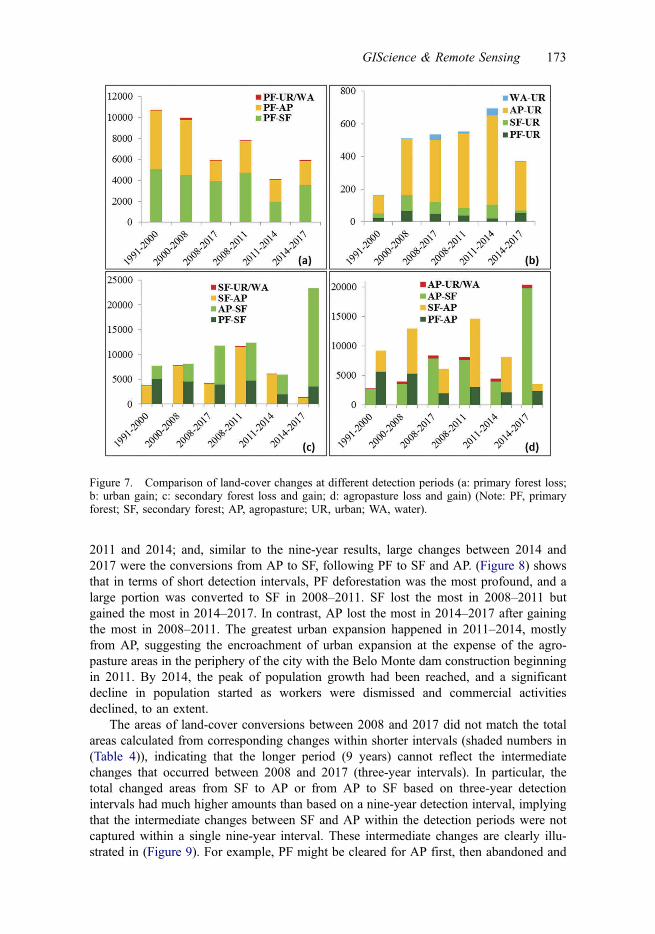
2011 and 2014; and, similar to the nine-year results, large changes between 2014 and2017 were the conversions from AP to SF, following PF to SF and AP. (Figure 8) showsthat in terms of short detection intervals, PF deforestation was the most profound, and alarge portion was converted to SF in 2008–2011. SF lost the most in 2008–2011 butgained the most in 2014–2017. In contrast, AP lost the most in 2014–2017 after gainingthe most in 2008–2011. The greatest urban expansion happened in 2011–2014, mostlyfrom AP, suggesting the encroachment of urban expansion at the expense of the agro-pasture areas in the periphery of the city with the Belo Monte dam construction beginningin 2011. By 2014, the peak of population growth had been reached, and a significantdecline in population started as workers were dismissed and commercial activitiesdeclined, to an extent.

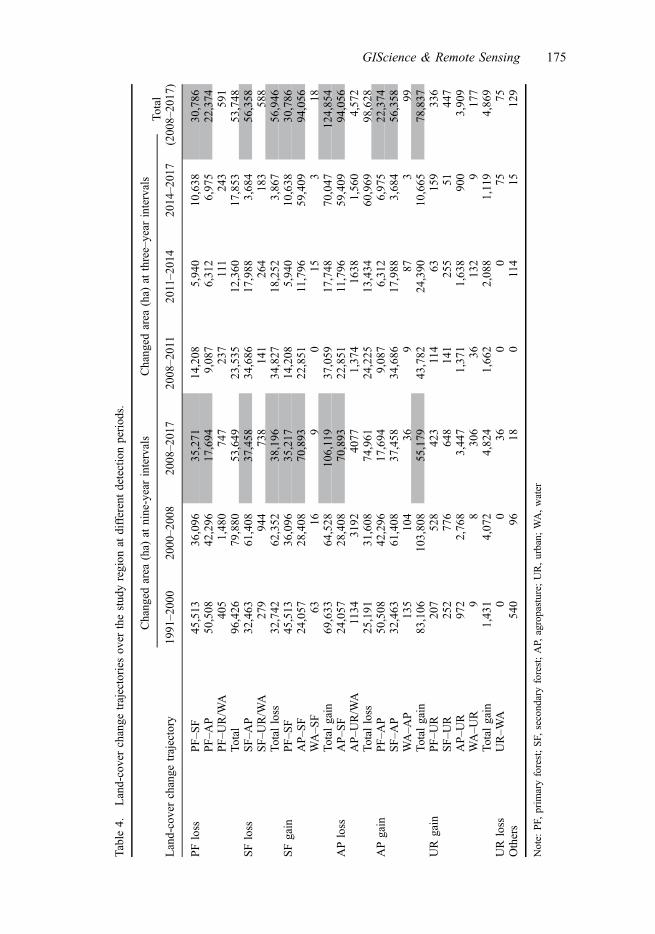
The areas of land-cover conversions between 2008 and 2017 did not match the totalareas calculated from corresponding changes within shorter intervals (shaded numbers in(Table 4)), indicating that the longer period (9 years) cannot reflect the intermediatechanges that occurred between 2008 and 2017 (three-year intervals). In particular, thetotal changed areas from SF to AP or from AP to SF based on three-year detectionintervals had much higher amounts than based on a nine-year detection interval, implyingthat the intermediate changes between SF and AP within the detection periods were notcaptured within a single nine-year interval. These intermediate changes are clearly illu-strated in (Figure 9). For example, PF might be cleared for AP first, then abandoned and

Figure 7. Comparison of land-cover changes at different detection periods (a: primary forest loss;b: urban gain; c: secondary forest loss and gain; d: agropasture loss and gain) (Note: PF, primaryforest; SF, secondary forest; AP, agropasture; UR, urban; WA, water).

GIScience & Remote Sensing 173

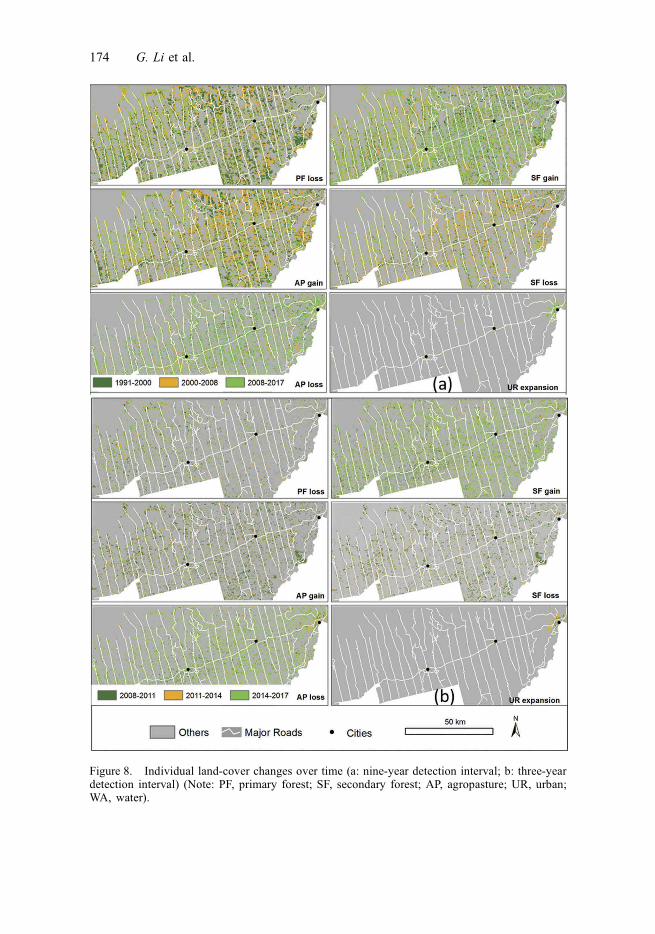
Figure 8. Individual land-cover changes over time (a: nine-year detection interval; b: three-yeardetection interval) (Note: PF, primary forest; SF, secondary forest; AP, agropasture; UR, urban;WA, water).

174 G. Li et al.

Table

4.Land-coverchange

trajectories

over

thestud

yregion

atdifferentdetectionperiod

s.

Land-coverchange

trajectory

Chang

edarea

(ha)

atnine-yearintervals

Chang

edarea

(ha)

atthree–year

intervals

Total

(200

8–20

17)

1991

–200

020

00–2

008

2008

–201

720

08–2

011

2011–201

420

14–2

017

PFloss

PF–S

F45

,513

36,096

35,271

14,208

5,94

010

,638

30,786

PF–A

P50

,508

42,296

17,694

9,08

76,31

26,97

522

,374

PF–U

R/W

A40

51,48

074

723

7111

243

591

Total

96,426

79,880

53,649

23,535

12,360

17,853

53,748

SFloss

SF–A

P32

,463

61,408

37,458

34,686

17,988

3,68

456

,358

SF–U

R/W

A27

994

473

814

126

418

358

8Total

loss

32,742

62,352

38,196

34,827

18,252

3,86

756

,946

SFgain

PF–S

F45

,513

36,096

35,217

14,208

5,94

010

,638

30,786

AP–S

F24

,057

28,408

70,893

22,851

11,796

59,409

94,056

WA–S

F63

169

015

318

Total

gain

69,633

64,528

106,119

37,059

17,748

70,047

124,85

4APloss

AP–S

F24

,057

28,408

70,893

22,851

11,796

59,409

94,056

AP–U

R/W

A1134

3192

4077

1,37

416

381,56

04,57

2Total

loss

25,191

31,608

74,961

24,225

13,434

60,969

98,628

APgain

PF–A

P50

,508

42,296

17,694

9,08

76,31

26,97

522

,374

SF–A

P32

,463

61,408

37,458

34,686

17,988

3,68

456

,358

WA–A

P13

510

436

987

399

Total

gain

83,106

103,80

855

,179

43,782

24,390

10,665

78,837

UR

gain

PF–U

R20

752

842

3114

6315

933

6SF–U

R25

277

664

814

125

551

447

AP–U

R97

22,76

83,44

71,37

11,63

890

03,90

9WA–U

R9

830

636

132

917

7Total

gain

1,43

14,07

24,82

41,66

22,08

81,119

4,86

9UR

loss

UR–W

A0

036

00

7575

Others

540

9618

0114

1512

9

Note:

PF,

prim

aryforest;SF,

secondaryforest;AP,

agropasture;

UR,urban;

WA,water

GIScience & Remote Sensing 175

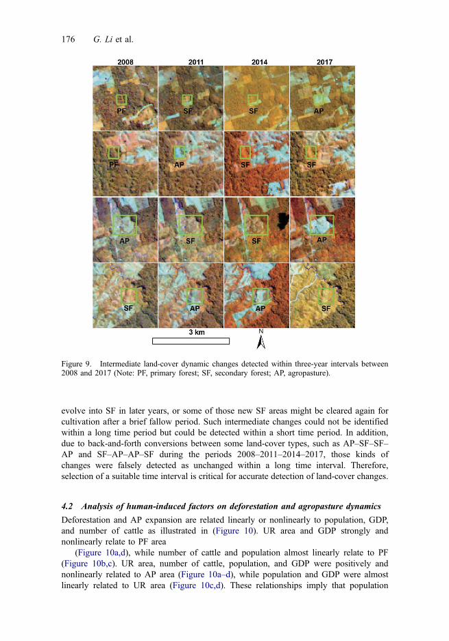
evolve into SF in later years, or some of those new SF areas might be cleared again forcultivation after a brief fallow period. Such intermediate changes could not be identifiedwithin a long time period but could be detected within a short time period. In addition,due to back-and-forth conversions between some land-cover types, such as AP–SF–SF–AP and SF–AP–AP–SF during the periods 2008–2011–2014–2017, those kinds ofchanges were falsely detected as unchanged within a long time interval. Therefore,selection of a suitable time interval is critical for accurate detection of land-cover changes.

4.2 Analysis of human-induced factors on deforestation and agropasture dynamics

Deforestation and AP expansion are related linearly or nonlinearly to population, GDP,and number of cattle as illustrated in (Figure 10). UR area and GDP strongly andnonlinearly relate to PF area

(Figure 10a,d), while number of cattle and population almost linearly relate to PF(Figure 10b,c). UR area, number of cattle, population, and GDP were positively andnonlinearly related to AP area (Figure 10a–d), while population and GDP were almostlinearly related to UR area (Figure 10c,d). These relationships imply that population

Figure 9. Intermediate land-cover dynamic changes detected within three-year intervals between2008 and 2017 (Note: PF, primary forest; SF, secondary forest; AP, agropasture).

176 G. Li et al.

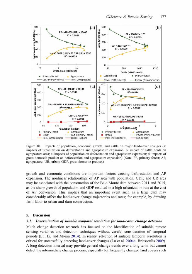
growth and economic conditions are important factors causing deforestation and APexpansion. The nonlinear relationships of AP area with population, GDP, and UR areamay be associated with the construction of the Belo Monte dam between 2011 and 2015,as the sharp growth of population and GDP resulted in a high urbanization rate at the costof AP conversion. This implies that an important event such as a large dam mayconsiderably affect the land-cover change trajectories and rates; for example, by drawingfarm labor to urban and dam construction.

5. Discussion

5.1. Determination of suitable temporal resolution for land-cover change detection

Much change detection research has focused on the identification of suitable remotesensing variables and detection techniques without careful consideration of temporalperiods (Lu, Li, and Moran 2014). In reality, selection of suitable temporal resolution iscritical for successfully detecting land-cover changes (Lu et al. 2004c; Briassoulis 2009).A long detection interval may provide general change trends over a long term, but cannotdetect the intermediate change process, especially for frequently changed land covers such

Figure 10. Impacts of population, economic growth, and cattle on major land-cover changes (a:impacts of urbanization on deforestation and agropasture expansion; b: impact of cattle herds onagropasture area; c: impacts of population on deforestation and agropasture expansion; d: impacts ofgross domestic product on deforestation and agropasture expansion) (Note: PF, primary forest; AP,agropasture; UR, urban; GDP, gross domestic product).

GIScience & Remote Sensing 177

as AP and SF in this study. In Brazil, the common practice of deforestation is peopleclearing trees for cattle ranching and crop farming by logging and burning. However, thesoil is rapidly degraded due to high temperatures and precipitation, and they may not beproductive for farming and ranching within a few years due to improper management (Luet al. 2004a, 2007). Thus, many lands are abandoned and convert to SF. After a coupleyears of soil recovery, these lands may be put back into production or AP. This requires usto carefully select temporal resolution to accurately capture the short-term land-coverchange. Because cocoa has higher economic value than pasture or cropland, there was alarge conversion from AP to cocoa in recent years, and we had to capture this change inthe short time intervals.

Many factors such as the availability of remotely sensed data, detection contents,characteristics of the study area, and time and labor involved in the detection work mayaffect this determination (Lu, Li, and Moran 2014). Some important events such as naturaldisasters and human-induced activities like selective logging require short-term changedetection intervals too. In this research, the El Niño problem in 2015/2016 may haveaffected land-cover change across a large area. The Belo Monte dam greatly affected theurban expansion of Altamira (Feng et al. 2017) and other land-cover changes near the damconstruction area. The political and economic conditions can also indirectly affect land-cover changes, requiring change detection to be conducted in a timely way.

Although this study indicates that a three-year interval provided more land-coverchange information than a nine-year interval, we cannot say this is the optimal timeperiod because of the difficulty in collecting a sufficient number of images. In recentyears, dense time-series Landsat images have been extensively applied to land-coverchange detection, especially to determine forest disturbances (Huang et al. 2010;Kennedy, Yang, and Cohen 2010; Zhu and Woodcock 2014; Hermosilla et al. 2016).However, land-cover change detection in the Brazilian Amazon basin has been difficultdue to cloud cover (Asner 2001), especially before 2000, when few sensor data besidesLandsat 5 and SPOT images were available. Although space-based radar data such asRadarsat C-band and ALOS PALSAR L-band are available, the poor separability in land-cover classes (Li et al. 2012), especially different forest types, makes them less successfulfor land-cover change detection. In recent years, more sensor data such as Sentinel-2 andLandsat 8 Operational Land Imager are available at no cost, and the application of GoogleEarth Engine technology provides a new platform for detecting detailed land-coverchange for short periods.

5.2. Forces driving land-cover change in the study region

The forces driving land-cover change have long been explored (Lambin 1997), but theyvary depending on the study areas, research scales (local or regional), and data avail-ability. It is necessary to understand the forces driving deforestation, urbanization, and APexpansion in the TransAmazon region. Previous research shows that population andeconomic conditions play important roles in urban expansion, and their influences aredependent upon the region and time (Kuang et al. 2014). For example, annual GDPgrowth per capita drove approximately half of observed urban land expansion in China,whereas urban population growth played a bigger role in India and Africa (Seto 2011).Population growth increases the demand for housing, supporting services, and facilities,resulting in urban expansion by converting vegetation and agricultural land to residentialuse, social and health care facilities, and infrastructure. This research also found popula-tion and economic growth were strongly related to deforestation and AP expansion. The

178 G. Li et al.

growth of population increases the demand for food supply, thus requiring more AP landsfor food and meat products, leading to AP expansion at the cost of PF deforestation. Inaddition to population growth, economic development creates demands for more housingspace, more goods and services, better education and medical facilities, and improvedinfrastructure, thus accelerating urban development. Economic development also drivesdeforestation of PF and AP expansion. Conversion of forest to AP for cattle ranching andagriculture is the most common route to achieving economic development in the Braziliancontext (Rodrigues et al. 2009). The strong relationship between number of cattle and AParea over time was indirectly conformed in Jusys (2016) that cattle ranching had thestrongest impact on deforestation across the Brazilian Amazon. Jusys (2016) also estab-lished that strong relationships between GDP and urban growth and deforestation meantthat high income was an accelerant of deforestation. Roads and highways have beenregarded as an important factor resulting in deforestation (Soares-Filho et al. 2004), andthis research showed that deforestation occurred along the roads in the early years.

The most rapid urban growth in our study area occurred during 2011–2014, coincidingwith the construction of Belo Monte Dam. During this period, an estimated 20,000 peoplewere relocated to Altamira after being removed from areas that would be flooded by thedam. At the same time, construction of the dam attracted a large number of migrantworkers and service providers to Altamira. Tremendous population growth in Altamirastimulated great urban expansion (Feng et al. 2017), and thus large areas of AP lands wereconverted to residential use. The nonlinear relationships of AP with UR, population, andGDP (Figure 10) can be attributed to the dam construction.

Our analyses found that SF area increased dramatically after 2014 and can be partiallyattributed to cocoa expansion. Brazil is one of the largest cocoa-producing countries, but itsproduction cannot meet even its own consumption and it has to import cocoa from others(Zugaib and Barreto 2015). Of the states in Brazil, Pará is the second-largest cocoa producer(Calvi, Augusto, and Araújo 2010). Recent government incentives promoting cocoa productionhave been extended to northern regions, like Pará, to stimulate its expansion. Cocoa plantationswere grouped into SF because of their spectral similarity, and the cocoa samples collected in thefield were actually located in areas classified as SF from remote sensing images.

6. Conclusions

This research examined land-cover dynamic change, especially deforestation and APdynamics, in the TransAmazon region in the northern Brazilian state of Pará usingmultitemporal Landsat imagery. We examined the impacts of human-induced factorssuch as population growth, economic condition, and cattle raising on deforestation andAP expansion. Our research confirmed that the hierarchical-based approach can success-fully classify the Landsat multispectral imagery into five land covers: PF, SF, AP, UR, andWA with an overall classification accuracy of 83.4%. PF linearly decreased from 1991 to2017, and AP linearly increased from 1991 to 2014, but sharply decreased from 2014 to2017. SF increased slightly from 1991 to 2000, remained stable between 2000 and 2014,then sharply increased from 2014 to 2017. UR increased linearly although it accounted fora very small proportion of change in this study area. Deforestation of PF accounted for alarge proportion of the land-cover change, especially before 2000, but the dynamicchanges between SF and AP became more important in the last decade. This researchindicates that a time interval of 9 years cannot effectively detect the dynamic changesbetween SF and AP and needs to be shorter, implying the necessity to identify suitabletemporal resolution in land-cover change detection. In addition to the common factors –

GIScience & Remote Sensing 179

population and economic conditions – affecting land-cover change, this research indicatesthat number of cattle and policies to expand cocoa plantations also affect deforestation andthe dynamic changes between SF and AP. Population growth associated with the con-struction of the dam led to urban expansion at the expense of AP. The Belo Monte damconstruction was an important factor resulting in AP and SF dynamic changes.

AcknowledgementsThis work was supported by the Fundação de Amparo a Pesquisa do Estado de São Paulo(processo 2012/51465-0), under the São Paulo Excellence Chairs Program, awarded to Emilio F.Moran as PI; US National Science Foundation under grant 1639115 to Moran as PI; MichiganState University through research funds provided to Dengsheng Lu and Emilio F. Moran.Luciano Vieira Dutra and Miquéias Freitas Calvi thank the Conselho Nacional deDesenvolvimento Científico e Tecnológico for supporting fieldwork through grants #401528/2012-0, #309135/2015-0, and #409936 2013-8.

Disclosure statementNo potential conflict of interest was reported by the authors.

FundingThis work was supported by the Fundação de Amparo à Pesquisa do Estado de São Paulo [2012/51465-0];National Science Foundation [1639115];Zhejiang Agriculture and Forestry University’sResearch and Development Fund [2013FR052];

ORCID

Guiying Li http://orcid.org/0000-0001-7198-4607

Dengsheng Lu http://orcid.org/0000-0003-4767-5710

Miquéias Freitas Calvi http://orcid.org/0000-0002-9409-9915

Luciano Vieira Dutra http://orcid.org/0000-0002-7757-039X

ReferencesAsner, G. P. 2001. “Cloud Cover in Landsat Observations of the Brazilian Amazon.” International

Journal of Remote Sensing 22 (18): 3855–3862. doi:10.1080/01431160010006926.Atkins, E. 2017. “Dammed and Diversionary: The Multi-Dimensional Framing of Brazil’s Belo

Monte Dam.” Singapore Journal of Tropical Geography 38 (3): 276–292. doi:10.1111/sjtg.12206.

Beuchle, R., R. C. Grecchi, Y. E. Shimabukuro, R. Seliger, H. D. Eva, E. Sano, and F. Achard. 2015.“Land Cover Changes in the Brazilian Cerrado and Caatinga Biomes from 1990 to 2010 Basedon a Systematic Remote Sensing Sampling Approach.” Applied Geography 58: 116–127.doi:10.1016/j.apgeog.2015.01.017.

Briassoulis, H. 2009. “Factors Influencing Land-Use and Land-Cover Change.” In: Encyclopedia ofLand Use, Land Cover and Soil Sciences: Land Cover, Land Use and Global Change, edited byW. H. Verhey. Encyclopedia of Life Support Systems (EOLSS) I:125–145. Oxford: EolssPublishers. URL https://www.eolss.net/TOC/C19-BrowseContents.aspx (membership required).

Brondízio, E. S. 2005. “Intraregional Analysis of Land-Use Change in the Amazon.” In Seeing theForest and the Trees: Human-Environment Interactions in Forest Ecosystems, edited by E. F.Moran and E. Ostrom, 223–252. Cambridge: MIT.

180 G. Li et al.

Calvi, M. F. 2009. “Fatores de adoção de sistemas agroflorestais por agricultores familiares domunicípio de Medicilândia, Pará.” Belém, Brasil: Universidade Federal do Pará. URL:https://ainfo.cnptia.embrapa.br/digital/bitstream/item/45741/1/AA-MIQUEIAS-FREITAS-CALVI.pdf.

Calvi, M. F., S. G. Augusto, and A. Araújo. 2010. Diagnóstico Do Arranjo Produtivo Local DaCultura Do Cacau No Território Da Transamazônica – Pará. Altamira: SEBRAE/UFPA.

Chander, G., B. L. Markham, and D. L. Helder. 2009. “Summary of Current RadiometricCalibration Coefficients for Landsat MSS, TM, ETM+, and EO-1 ALI Sensors.” RemoteSensing of Environment 113 (5): 893–903. doi:10.1016/j.rse.2009.01.007.

Chávez, P. S. Jr. 1996. “Image-Based Atmospheric Corrections – Revisited and Improved.”Photogrammetric Engineering and Remote Sensing 62 (9): 1025–1036. 0099-1112/96/6209-1025.

Chen, G., R. P. Powers, L. M. T. De Carvalho, and B. Mora. 2015. “Spatiotemporal Patterns ofTropical Deforestation and Forest Degradation in Response to the Operation of the TucuruíHydroelectric Dam in the Amazon Basin.” Applied Geography 63: 1–8. doi:10.1016/j.apgeog.2015.06.001.

Congalton, R. G., and K. Green. 2009. Assessing the Accuracy of Remotely Sensed Data: Principlesand Practices. Boca Raton: CRC Press/Taylor & Francis.

Fearnside, P. M. 2016. “Environmental and Social Impacts of Hydroelectric Dams in BrazilianAmazonia: Implications for the Aluminum Industry.” World Development 77: 48–65.doi:10.1016/J.WORLDDEV.2015.08.015.

Feng, Y., D. Lu, E. F. Moran, L. V. Dutra, M. F. Calvi, and M. A. F. Oliveira. 2017. “ExaminingSpatial Distribution and Dynamic Change of Urban Land Covers in the Brazilian AmazonUsing Multitemporal Multisensor High Spatial Resolution Satellite Imagery.” Remote Sensing 9(4): 381. doi:10.3390/rs9040381.

Foody, G. M. 2002. “Status of Land Cover Classification Accuracy Assessment.” Remote Sensing ofEnvironment 80 (1): 185–201. doi:10.1016/S0034-4257(01)00295-4.

Government, B. 2017. Investment Guide to Brasil 2017. URL: https://investexportbrasil.dpr.gov.br/Arquivos/Publicacoes/Estudos/InvestmentGuide2017.pdf.

Grecchi, R. C., R. Beuchle, Y. E. Shimabukuro, L. E. O. C. Aragão, E. Arai, D. Simonetti, and F.Achard. 2017. “An Integrated Remote Sensing and GIS Approach for Monitoring AreasAffected by Selective Logging: A Case Study in Northern Mato Grosso, Brazilian Amazon.”International Journal of Applied Earth Observation and Geoinformation 61: 70–80.doi:10.1016/j.jag.2017.05.001.

Grecchi, R. C., Q. H. J. Gwyn, G. B. Bénié, A. R. Formaggio, and F. C. Fahl. 2014. “Land Use and LandCover Changes in the Brazilian Cerrado: A Multidisciplinary Approach to Assess the Impacts ofAgricultural Expansion.” Applied Geography 55: 300–312. doi:10.1016/j.apgeog.2014.09.014.

Hermosilla, T., M. A. Wulder, J. C. White, N. C. Coops, G. W. Hobart, and L. B. Campbell. 2016.“Mass Data Processing of Time Series Landsat Imagery: Pixels to Data Products for ForestMonitoring.” International Journal of Digital Earth 9 (11): 1035–1054. doi:10.1080/17538947.2016.1187673.

Huang, C., S. N. Goward, J. G. Masek, N. Thomas, Z. Zhu, and J. E. Vogelmann. 2010. ““AnAutomated Approach for Reconstructing Recent Forest Disturbance History Using DenseLandsat Time Series Stacks.” Remote Sensing of Environment 114 (1): 183–198. doi:10.1016/j.rse.2009.08.017.

Imbach, P., M. Manrow, E. Barona, A. Barretto, G. Hyman, and P. Ciais. 2015. “Spatial andTemporal Contrasts in the Distribution of Crops and Pastures across Amazonia: A NewAgricultural Land Use Data Set from Census Data since 1950.” Global BiogeochemicalCycles 29 (6): 898–916. doi:10.1002/2014GB004999.

Jusys, T. 2016. “Fundamental Causes and Spatial Heterogeneity of Deforestation in Legal Amazon.”Applied Geography 75: 188–199. doi:10.1016/j.apgeog.2016.08.015.

Karathanassi, V., P. Kolokousis, and S. Ioannidou. 2007. “A Comparison Study on Fusion MethodsUsing Evaluation Indicators.” International Journal of Remote Sensing 28 (10): 2309–2341.doi:10.1080/01431160600606890.

Kennedy,R. E., Z.Q.Yang, andW.B.Cohen. 2010. “DetectingTrends in ForestDisturbance andRecoveryUsing Yearly Landsat Time Series: 1. LandTrendr - Temporal Segmentation Algorithms.” RemoteSensing of Environment 114 (12): 2897–2910. doi:10.1016/j.rse.2010.07.008.

GIScience & Remote Sensing 181

Kuang, W., W. Chi, D. Lu, and Y. Dou. 2014. “A Comparative Analysis of Megacity Expansions inChina and the U.S.: Patterns, Rates and Driving Forces.” Landscape and Urban Planning 132:121–135. doi:10.1016/j.landurbplan.2014.08.015.

Lambin, E. F. 1997. “Modelling and Monitoring Land-Cover Change Processes in Tropical Regions.”Progress in Physical Geography 21 (3): 375–393. doi:10.1177/030913339702100303.

Li, G., D. Lu, E. Moran, and S. Hetrick. 2011. “Land-Cover Classification in a Moist TropicalRegion of Brazil with Landsat Thematic Mapper Imagery.” International Journal of RemoteSensing 32 (23): 8207–8230. doi:10.1080/01431161.2010.532831.

Li, G., D. Lu, E. Moran, and S. J. S. Sant’Anna. 2012. “Comparative Analysis of ClassificationAlgorithms and Multiple Sensor Data for Land Use/Land Cover Classification in the BrazilianAmazon.” Journal of Applied Remote Sensing 6 (1): 061706. doi:10.1117/1.JRS.6.061706. Dec14, 2012.

Lu, D., M. Batistella, P. Mausel, and E. Moran. 2007. “Mapping and Monitoring Land DegradationRisks in the Western Brazilian Amazon Using Multitemporal Landsat TM/ETM+ Images.”Land Degradation and Development 18 (1): 41–54. doi:10.1002/ldr.762.

Lu, D., S. Hetrick, E. Moran, and G. Li. 2010. “Detection of Urban Expansion in an Urban-RuralLandscape with Multitemporal QuickBird Images.” Journal of Applied Remote Sensing 4:041880. doi:10.1117/1.3501124.

Lu, D., S. Hetrick, E. Moran, and G. Li. 2012. “Application of Time Series Landsat Images toExamining Land-use/Land-Cover Dynamic Change.” Photogrammetric Engineering & RemoteSensing 78 (7): 747–755. doi:10.14358/PERS.78.7.747.

Lu, D., G. Li, and E. Moran. 2014. “Current Situation and Needs of Change Detection Techniques.”International Journal of Image and Data Fusion 5: 13–38. doi:10.1080/19479832.2013.868372.

Lu, D., G. Li, E. Moran, and S. Hetrick. 2013. “Spatiotemporal Analysis of Land-Use and Land-Cover Change in the Brazilian Amazon.” International Journal of Remote Sensing 34 (16):5953–5978. doi:10.1080/01431161.2013.802825.

Lu, D., G. Li, G. S. Valladares, and M. Batistella. 2004a. “Mapping Soil Erosion Risk in Rondônia,Brazilian Amazonia: Using Rusle, Remote Sensing and GIS.” Land Degradation &Development 15: 499–512. doi:10.1002/ldr.634.

Lu, D., P. Mausel, M. Batistella, and E. Moran. 2004b. “Comparison of Land-Cover ClassificationMethods in the Brazilian Amazon Basin.” Photogrammetric Engineering & Remote Sensing 70(6): 723–731. doi:10.14358/PERS.70.6.723.

Lu, D., P. Mausel, E. Brondízio, and E. Moran. 2004c. “Change Detection Techniques.” InternationalJournal of Remote Sensing 25 (12): 2365–2407. doi:10.1080/0143116031000139863.

Moran, E. F. 1975. “The Brazilian Colonization Experience in the Transamazon Highway.” Papersin Anthropology 16 (1): 29–57.

Moran, E. F. 1981. Developing the Amazon. Bloomington: Indiana University Press.Moran, E. F. 2016. “Roads and Dams: Infrastructure-Driven Transforamtions in the Brazilian Amazon.”

Ambiente & Sociedade 19 (2): 207–220. doi:10.1590/1809-4422ASOC256V1922016.Moran, E. F., and E. Brondizio. 1998. “Land-Use Change after Deforestation in Amazonia.” In

People and Pixels: Linking Remote Sensing and Social Science, edited by D. Liverman, E. F.Moran, R. R. Rindfuss, and P. Stern, 94–120. Washington, DC: National Academies Press.

Moran, E. F., E. Brondizio, P. Mausel, and Y. Wu. 1994. “Integrating Amazonian Vegetation, Land-Use, and Satellite Data.” BioScience 44 (5): 329–338. doi:10.2307/1312383.

Müller, H., P. Griffiths, and P. Hostert. 2016. “Long-Term Deforestation Dynamics in the BrazilianAmazon—Uncovering Historic Frontier Development along the Cuiabá–Santarém Highway.”International Journal of Applied Earth Observation and Geoinformation 44: 61–69.doi:10.1016/j.jag.2015.07.005.

Ritter, C. D., G. McCrate, R. H. Nilsson, P. M. Fearnside, U. Palme, and A. Antonelli. 2017.“Environmental Impact Assessment in Brazilian Amazonia: Challenges and Prospects to AssessBiodiversity.” Biological Conservation 206: 161–168. doi:10.1016/j.biocon.2016.12.031.

Rodrigues, A. S. L., R. M. Ewers, L. Parry, C. Souza, A. Veríssimo, and A. Balmford. 2009.“Boom-and-Bust Development Patterns across the Amazon Deforestation Frontier.” Science 324(5933): 1435–1437. doi:10.1126/science.1174002.

Schneibel, A., D. Frantz, A. Röder, M. Stellmes, K. Fischer, and J. Hill. 2017. “Using AnnualLandsat Time Series for the Detection of Dry Forest Degradation Processes in South-CentralAngola.” Remote Sensing 9 (9): 905. doi:10.3390/rs9090905.

182 G. Li et al.

Seto, K. C. 2011. “Exploring the Dynamics of Migration to Mega-Delta Cities in Asia and Africa:Contemporary Drivers and Future Scenarios.” Global Environmental Change 21 (SUPPL. 1):94–107. doi:10.1016/j.gloenvcha.2011.08.005.

Shimizu, K., R. Ponce-Hernandez, O. S. Ahmed, T. Ota, Z. C. Win, N. Mizoue, and S. Yoshida.2017. “Using Landsat Time Series Imagery to Detect Forest Disturbance in Selectively LoggedTropical Forests in Myanmar.” Canadian Journal of Forest Research 47: 289–296. doi:10.1139/cjfr-2016-0244.

Silveira, E. M. O., J. M. Mello, F. W. Acerbi Jr, and L. M. T. Carvalho. 2018. “Object-Based Land-Cover Change Detection Applied to Brazilian Seasonal Savannahs Using GeostatisticalFeatures.” International Journal of Remote Sensing 39 (8): 2597–2619. doi:10.1080/01431161.2018.1430397.

Soares-Filho, B., A. Alencar, D. Nepstad, G. Cerqueira, M. D. C. Vera Diaz, S. Rivero, L.Solórzano, and E. Voll. 2004. “Simulating the Response of Land-Cover Changes to RoadPaving and Governance along a Major Amazon Highway: The Santarém-Cuiabá Corridor.”Global Change Biology 10 (5): 745–764. doi:10.1111/j.1529-8817.2003.00769.x.

Spera, S. A., A. S. Cohn, L. K. Vanwey, J. F. Mustard, B. F. Rudorff, J. Risso, and M. Adami. 2014.“Recent Cropping Frequency, Expansion, and Abandonment in Mato Grosso, Brazil HadSelective Land Characteristics.” Environmental Research Letters 9: 064010. doi:10.1088/1748-9326/9/6/064010.

Tucker, J. M., E. S. Brondizio, and E. F. Morán. 1998. “Rates of Forest Regrowth in EasternAmazónia: A Comparison of Altamira and Bragantina Regions, Pará State, Brazil.” Interciencia23: 64–73.

Tundisi, J. G., T. Matsumura-Tundisi, and J. E. Tundisi. 2015. “Environmental Impact Assessmentof Reservoir Construction: New Perspectives for Restoration Economy, and Development: TheBelo Monte Power Plant Case Study.” Brazilian Journal of Biology 75 (3 suppl 1): 10–15.doi:10.1590/1519-6984.03514BM.

Walker, R., and A. K. O. Homma. 1996. “Land Use and Land Cover Dynamics in the BrazilianAmazon: An Overview.” Ecological Economics 18 (1): 67–80. doi:10.1016/0921-8009(96)00033-X.

Walker, R., E. Moran, and L. Anselin. 2000. “Deforestation and Cattle Ranching in the BrazilianAmazon: External Capital and Household Processes.” World Development 28 (4): 683–699.doi:10.1016/S0305-750X(99)00149-7.

Zhu, Z., and C. E. Woodcock. 2014. “Continuous Change Detection and Classification of LandCover Using All Available Landsat Data.” Remote Sensing of Environment 144: 152–171.doi:10.1016/j.rse.2014.01.011.

Zugaib, A. C. C., and R. C. S. Barreto. 2015. “O mercado Brasileiro de cacau: Perspectivas de demanda,oferta e preços.” Agrotrópica 27 (3): 303–316. doi:10.21757/0103-3816.2015v27n3p303-316.

GIScience & Remote Sensing 183