Exercise 7. Royle-Nichols Abundance Induced … in Occupancy Estimation and Modeling; Donovan and Hines 2007 Chapter 7 Page 1 5/8/2007 EXERCISE 7: ROYLE-NICHOLS ABUNDANCE INDUCED

Exercises in Occupancy Estimation and Modeling; Donovan and Hines 2007

Chapter 7 Page 1 5/8/2007

EXERCISE 7: ROYLE-NICHOLS ABUNDANCE INDUCED HETEROGENEITY

Estimating mean abundance from repeated presence-absence surveys

In collaboration with Kurt Rinehart, University of Vermont, Rubenstein

School of Environment and Natural Resources

Please cite this work as: Donovan, T. M. and J. Hines. 2007. Exercises in

occupancy modeling and estimation.

<http://www.uvm.edu/envnr/vtcfwru/spreadsheets/occupancy.htm



TABLE OF CONTENTS

OBJECTIVES ..............................................................................................................3 INTRODUCTION .......................................................................................................3 THE PRIOR DISTIBUTION ..................................................................................6 THE POISSON DISTRIBUTION .........................................................................7 PROBABILITY OF DETECTING AN ANIMAL AT A SITE ........................11 KEY ASSUMPTIONS OF THE ROYLE-NICHOLS MODEL ........................ 14 THE ROYLE-NICHOLS MODEL OVERVIEW.................................................. 14 MIXTURE MODEL BASICS.................................................................................. 16 THE ROYLE-NICHOLS LIKELIHOOD OVERVIEW ...................................... 19 THE LIKELIHOOD FOR A SINGLE SITE ..................................................... 20 THE ROYLE-NICHOLS LIKELIHOOD FOR ALL SITES ........................... 24 THE ROYLE-NICHOLS SPREADSHEET MODEL INPUTS ........................ 25 THE LIKELIHOOD FOR SITES, ONE AT A TIME ................................... 28 RUNNING THE MODEL ....................................................................................... 34 MAXIMIZING THE LIKELIHOOD ................................................................... 36 INTERPRETING THE MODEL OUTPUT ......................................................... 37 SIMULATING DATA............................................................................................. 38 SOME ADDITIONAL THINGS TO PONDER ................................................ 42 GETTING STARTED.............................................................................................. 45 RUNNING THE ROYLE-NICHOLS MODEL ................................................... 47 THE ROYLE-NICHOLS OUTPUT ...................................................................... 48



OBJECTIVES

• To understand the basics of the Poisson and Binomial distributions.

• To learn and understand the basic mixture model for estimating

abundance, and how it fits into a multinomial maximum likelihood

analysis.

• To use Solver to find the maximum likelihood estimates for the

probability of detection and lambda, the average site abundance.

• To assess deviance of the saturated model.

• To introduce concepts of model fit.

• To learn how to simulate basic mixture data.

INTRODUCTION Suppose that you want to estimate the size of an animal population. For one

reason or another, you are not able to employ standard population estimation

techniques like capture-recapture or distance sampling, so instead you

gather presence-absence data (or more properly, detection-non detection

data). Your data could be detections of some insect species found on crop

plants, detections of a singing bird species, or secondary sign counts of

mammals. Let’s suppose you are interested in the abundance of a particular

mammalian carnivore. On each visit, you search for fresh sign (tracks,

feces, etc.). You see some scat and some fresh tracks at two different spots

within a site. Are they from the same or different individuals? You can’t tell

because the animals are not marked. Another situation might involve remote

camera surveys for a species, in which all the individuals look the same: 3

pictures could be from 3, 2, or just 1 individual. In both examples, you can’t

correlate the number of signs to the number of animals because one animal



may have produced many signs; you can only record the detection or non-

detection of the species.

Because you can’t sample individuals, you will sample the area itself. You

check to see if the site is occupied by the species of interest and record any

signs at that site as a single detection. This is an occupancy survey. You

won’t do it just once - you’ll go back for repeated visits and record detection

or non-detection at each subsequent visit. The detection history at a site

will be recorded as a sequence of 1’s and 0’s (1 = detection, 0 = no detection)

across the sample periods. Let’s let T equal the total number of visits. An

example encounter history for a site sampled 5 times (T = 5) might be 00110.

There were no detections in either of the first two visits, detections for

visits three and four, and no detection again on the fifth visit.

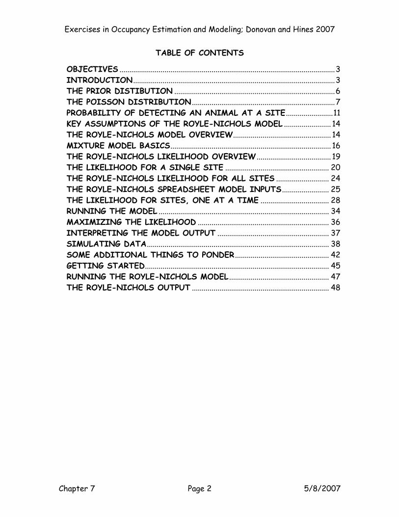
Now let’s suppose you sample a number of different sites in your study area.

Let R equal the total number of sites that are surveyed. At each of the R

sites, you will determine whether or not you detect your target species at

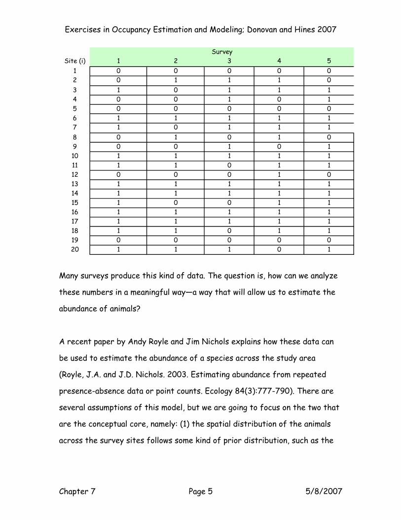
each time interval. Here is a sample data sheet for a survey of 20 sites (R =

20), each sampled on 5 different occasions (T = 5):



Site (i) 1 2 3 4 51 0 0 0 0 02 0 1 1 1 03 1 0 1 1 14 0 0 1 0 15 0 0 0 0 06 1 1 1 1 17 1 0 1 1 18 0 1 0 1 09 0 0 1 0 110 1 1 1 1 111 1 1 0 1 112 0 0 0 1 013 1 1 1 1 114 1 1 1 1 115 1 0 0 1 116 1 1 1 1 117 1 1 1 1 118 1 1 0 1 119 0 0 0 0 020 1 1 1 0 1

Survey

Many surveys produce this kind of data. The question is, how can we analyze

these numbers in a meaningful way—a way that will allow us to estimate the

abundance of animals?

A recent paper by Andy Royle and Jim Nichols explains how these data can

be used to estimate the abundance of a species across the study area

(Royle, J.A. and J.D. Nichols. 2003. Estimating abundance from repeated

presence-absence data or point counts. Ecology 84(3):777-790). There are

several assumptions of this model, but we are going to focus on the two that

are the conceptual core, namely: (1) the spatial distribution of the animals

across the survey sites follows some kind of prior distribution, such as the



Poisson distribution, and (2) the probability of detecting an animal at a site

is a function of how many animals are actually at that site.

Note that the Royle-Nichols model can accommodate different kinds of

distributions representing the spatial distribution of the target species, but

that we will focus exclusively on the Poisson distribution in this exercise. We

use the Poisson in our spreadsheet and, for simplicity, we may omit

reference to the fact that the Poisson is simply one option for modeling

spatial distribution. This should become clearer after we discuss these

assumptions in depth. After that, we’ll go through how the Royle-Nichols

model is put together.

THE PRIOR DISTIBUTION

In the Royle-Nichols model, we must “specify” a “prior” spatial distribution

of the abundance of our target species. The spatial distribution of animals is

simply how many animals occur at each site within the study area. However

they are distributed, each of the survey sites will contain some number of

animals (some sites may contain 0 animals). That number, the site abundance,

is a function of the mechanisms governing the distribution.

A prior distribution is specified, or chosen, based on how you think the

animal species is really distributed. If you were in the planning stages of

your survey and had not yet collected any data, you would ask yourself, “How

are these animals distributed in space?” Prior to collecting any data, we

specify the Poisson—we consider the Poisson to accurately represent the

true spatial distribution of our target species. Alternatively, prior studies



might suggest that the Poisson is an appropriate distribution to use. We

choose the Poisson probability function to represent the mechanisms of the

spatial distribution. The Poisson won’t tell us exactly how many animals

inhabit a site, but it will define the probability for any number you might

choose to consider. Let’s start by reviewing the Poisson Distribution, and

then we can see how it is used in the Royle-Nichols model.

THE POISSON DISTRIBUTION

The Poisson distribution is used to model the number of certain randomly

occurring events, like the number of car accidents in your home town, or the

number of individuals of a species within each of your survey sites. In the

car accident example, each accident is independent of every other accident

and the number of accidents in any time period is random and independent of

any other time period. The spatial distribution of animals can also meet

these Poisson assumptions when the number of animals inhabiting one site is

random and independent of the number of animals at other sites.

The Royle-Nichols model assumes that each of the R sites in your occupancy

survey is home to some number of animals that can be modeled by a

specified prior distribution like the Poisson. In essence, each site is home to

a certain number of animals of your target species and that number is a

function of the specified process. We also must assume this number does

not change over the course of your study. The population must be

demographically closed, meaning that the number of individuals at the site

does not change across sampling periods. That is, no births, no deaths, no



immigrants, no emigrants. This additional assumption means repeated

sampling visits must be completed within a relatively short period of time.

The Poisson distribution has a single parameter, λ (“lambda”), the mean. In

this case, lambda is the mean abundance across the R sites. The Poisson

distribution returns the probability of any level of abundance x from 0 to ∞

given some lambda. Suppose you win a huge grant ($$) and can accurately

count the number of animals within your study area (instead of collecting

presence-absence data). You can take this total abundance and divide it by

the number of survey sites in the study area, R, and find that the mean

abundance is 3 animals per site (lambda = 3). Suppose further, that you

know (or assume) the number of animals in any site follows a Poisson

distribution. Given this information, you can find the probability that a

specific number of animals will occur at a given site. For example, when

lambda = 3, the probability of a single site having an abundance of 5 is 0.10.

Where does 0.10 come from? It is calculated with the probability density

formula for the Poisson:

where lambda is the mean of the Poisson distribution, and x is the “event” of

interest, which in this case is the number of animals at a given site: x = 5.

(Note: “fx” is a generic term for any probability distribution. The term to

!xef

x

xλλ−

=



the right of the equals sign is unique to the Poisson.) If you calculate this

function for lambda = 3 and x = 5 animals, the result is a probability of 0.10.

10.01*2*3*4*5

3)3exp( 5

5 =−

=f

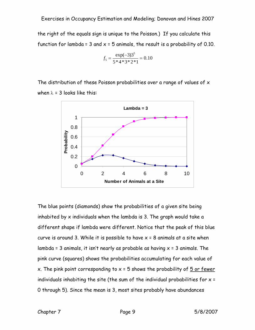
The distribution of these Poisson probabilities over a range of values of x

when λ = 3 looks like this:

Lambda = 3

0

0.2

0.4

0.6

0.8

1

0 2 4 6 8 10Number of Animals at a Site

Prob

abili

ty

The blue points (diamonds) show the probabilities of a given site being

inhabited by x individuals when the lambda is 3. The graph would take a

different shape if lambda were different. Notice that the peak of this blue

curve is around 3. While it is possible to have x = 8 animals at a site when

lambda = 3 animals, it isn’t nearly as probable as having x = 3 animals. The

pink curve (squares) shows the probabilities accumulating for each value of

x. The pink point corresponding to x = 5 shows the probability of 5 or fewer

individuals inhabiting the site (the sum of the individual probabilities for x =

0 through 5). Since the mean is 3, most sites probably have abundances



around 3 so the cumulative probability for x = 5 is quite high (0.92, in fact).

It’s easy to generate such probabilities in Excel with the POISSON

function. In this function, you enter x and lambda, and then tell Excel

whether you want the cumulative probability (“true”) or individual probability

(“false”). For example, we used “=Poisson(5,3,true)” to obtain the cumulative

probability of 0.92 mentioned above.

Here are some more examples of interpretation of the Poisson distribution

and its single parameter, lambda. Look again at the graph above. Lambda = 3

indicates that the average abundance for all sites is 3. Many sites will have

3 animals. When lambda = 3, x = 3 has the highest probability of occurrence.

There will be quite a few sites with 0, 1, 2, 4, and 5 animals, and fewer sites

with more than 5 animals.

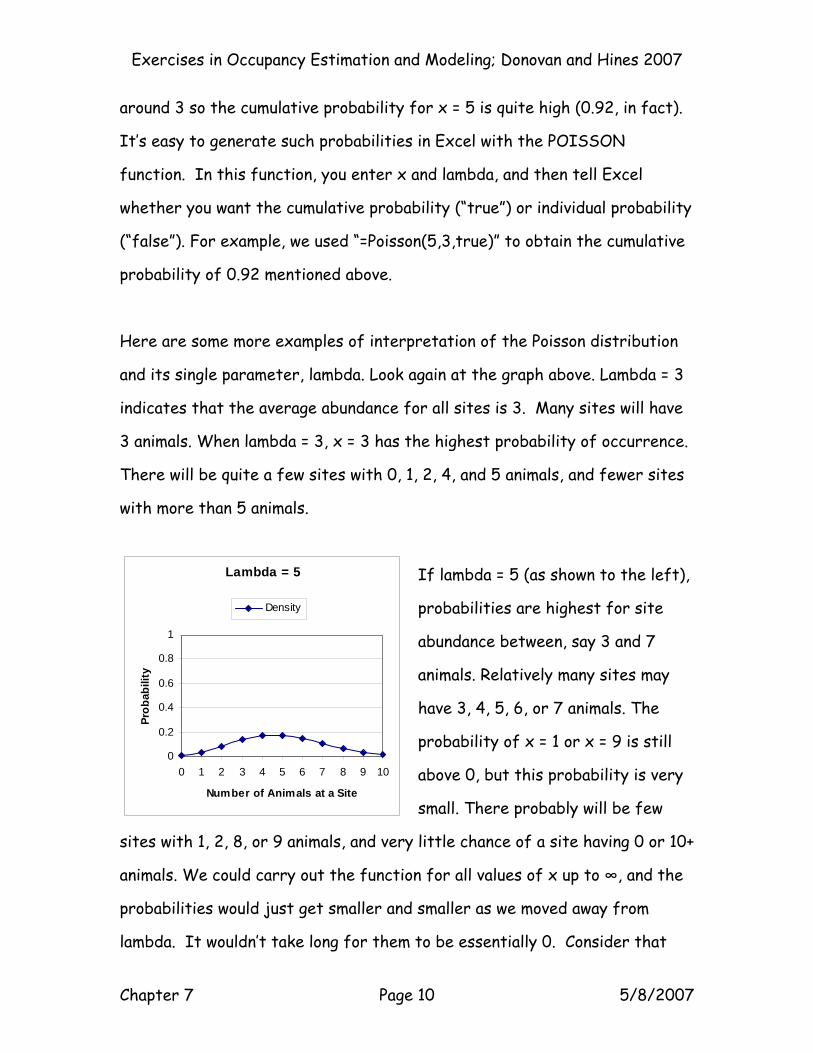
If lambda = 5 (as shown to the left),

probabilities are highest for site

abundance between, say 3 and 7

animals. Relatively many sites may

have 3, 4, 5, 6, or 7 animals. The

probability of x = 1 or x = 9 is still

above 0, but this probability is very

small. There probably will be few

sites with 1, 2, 8, or 9 animals, and very little chance of a site having 0 or 10+

animals. We could carry out the function for all values of x up to ∞, and the

probabilities would just get smaller and smaller as we moved away from

lambda. It wouldn’t take long for them to be essentially 0. Consider that

Lambda = 5

0

0.2

0.4

0.6

0.8

1

0 1 2 3 4 5 6 7 8 9 10

Number of Animals at a Site

Prob

abili

ty

Density



for lambda = 5 as in the graph above, the Poisson probability of x = 10 is

0.018. For x = 20 it is 0.00000027. It’s very unlikely that a site would have

20 animals when lambda = 5.

The intent behind all of this is to “define” the function we will use to

calculate the probability of a given level of abundance at any site. Why do

we care? Because the Royle-Nichols model assumes that whether an animal is

detected at a site is a function of site abundance (more on this in a bit). We

need to know how likely one abundance is relative to another. Without

specifying a prior distribution, we would be saying, in effect, “We think any

number of animals at this site is as likely as any other number. A site

abundance of 2 is as likely as 20.” This is not only uninformative, it’s totally

unrealistic. Spatial distributions of organisms do follow mechanisms that can

be represented by probability distributions. By specifying a prior

distribution, we can quantify the probabilities of site abundance being 2 or

20. For the Poisson, we can do this provided we know the average abundance

across all sites. In practice, we won’t know true abundances, so lambda is

one of the key parameters that is estimated by Royle-Nichols model.

PROBABILITY OF DETECTING AN ANIMAL AT A SITE

The second major assumption of the Royle-Nichols model is related to the

first: the probability of detection of our target species at any site is a

function of the abundance of animals there. But before we go there, let’s

step back for a moment and think about detection probability. All animals

have some inherent detection probability that is independent of abundance.

Some species are easy to find and locate, while others (cougars, for



example) are just plain difficult to observe. Royle and Nichols call this

inherent detection probability, r. This varies by species, but is constant for

all individuals of a species. Cougars may have an r of 0.1, while black-

throated blue warblers during the breeding season may have a detection

probability of 0.8. A typical occupancy model such as the single-season

model (MacKenzie et al. 2002) aims to estimate this detection probability in

order to estimate the number of sites that were truly occupied even if

there were no detections there.

Royle and Nichols take this concept one step further. Recall that we are

sampling sites, not individuals. Our detections will not purely reflect the r

of the target species; they will follow a site detection probability that is a

function of r and the site abundance.

For a given species detectability, r, it’s easier to achieve detection when

there are many animals at the site than when there are few. Even though

cougars are inherently difficult to detect, you are more likely to observe

cougar sign when a site is occupied by 10 cougars compared to 1. To record a

detection for the site, you need only detect a single individual of those that

are present. To fail to detect, you need to miss every individual. The more

individuals are present, the more chances you have to detect them. Since you

ensure that your surveys all fall within a period of time over which you can

assume that the site abundance does not change (demographic closure), the

probability of detection at the site follow this formula:

iNrp )1(1 −−=



This “site detection probability”, p, is a function of the species inherent

detection probability, r, and the site abundance, Ni. (NOTE: Ni is the

abundance at site i.) We’ll let Ntotal represent the total abundance across all

sites. Ntotal = Σ(Ni). The term (1-r) is the probability of missing a single

individual occupying the site. The probability of missing all Ni individuals is

(1-r)Ni. Thus, the probability of detecting any animal at the site is one minus

this term, or 1 –(1-r)Ni.

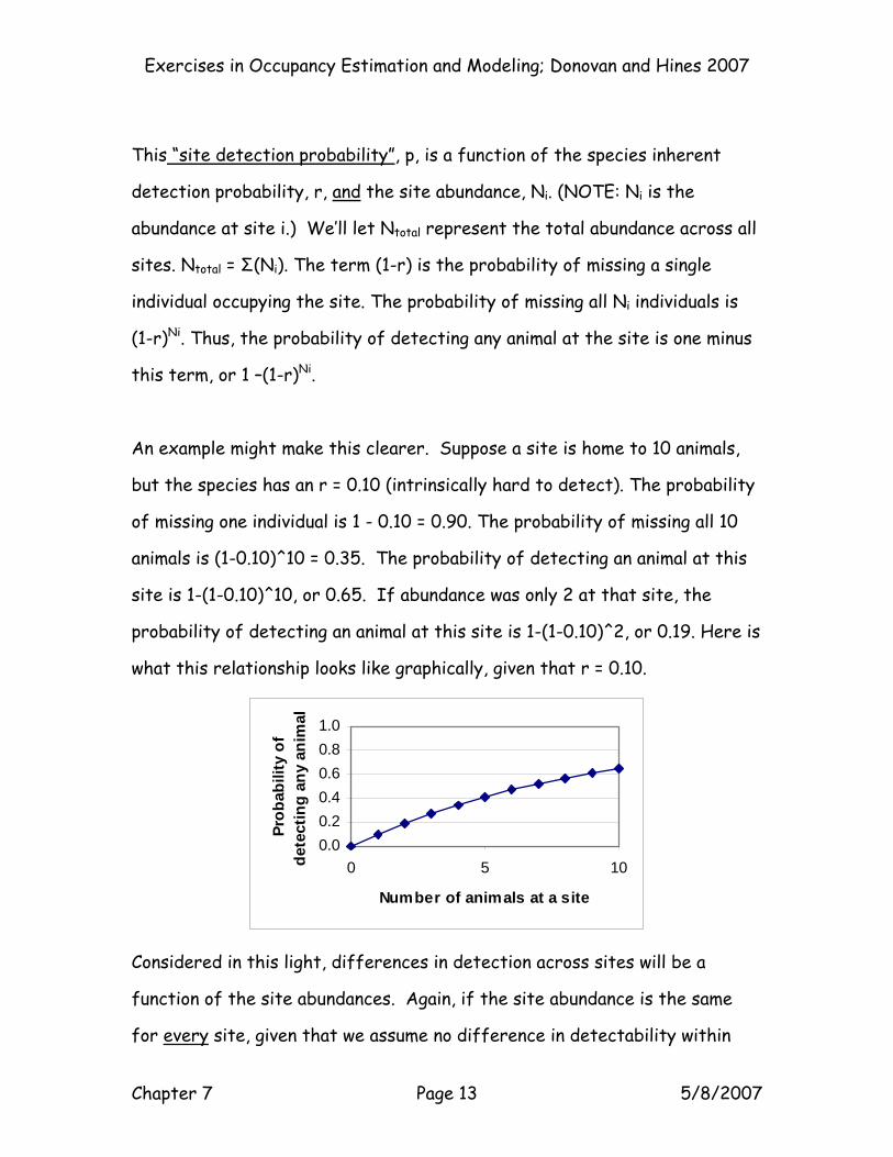
An example might make this clearer. Suppose a site is home to 10 animals,

but the species has an r = 0.10 (intrinsically hard to detect). The probability

of missing one individual is 1 - 0.10 = 0.90. The probability of missing all 10

animals is (1-0.10)^10 = 0.35. The probability of detecting an animal at this

site is 1-(1-0.10)^10, or 0.65. If abundance was only 2 at that site, the

probability of detecting an animal at this site is 1-(1-0.10)^2, or 0.19. Here is

what this relationship looks like graphically, given that r = 0.10.

0.00.20.40.60.81.0

0 5 10

Number of animals at a site

Prob

abili

ty o

f de

tect

ing

any

anim

al

Considered in this light, differences in detection across sites will be a

function of the site abundances. Again, if the site abundance is the same

for every site, given that we assume no difference in detectability within



the species, then you would expect the detections to be equal among the

sites. Conversely, heterogeneous detectability (differences in the total

detections per site) implies different site abundances.

KEY ASSUMPTIONS OF THE ROYLE-NICHOLS MODEL

OK, to recap: The key assumptions of the Royle-Nichols model are that (1)

the number of animals at a particular site follows a Poisson probability

distribution for which lambda indicates the mean abundance across all sites,

and (2) the probability of detecting animals at each site is related to the

species’ r and the site abundance, Ni.

THE ROYLE-NICHOLS MODEL OVERVIEW

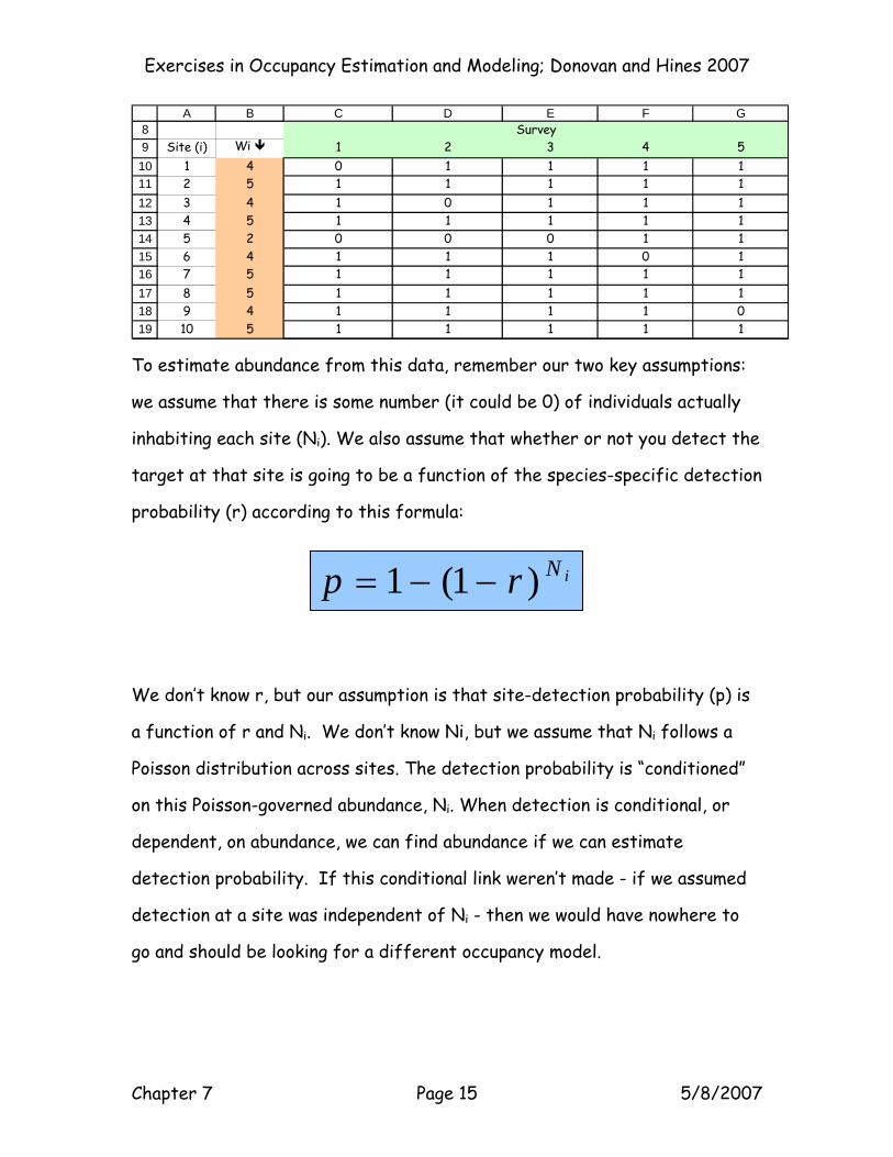
As with other occupancy models, repeated surveys are the cornerstone of

data collection. For each site in your survey, you will get a series of 1’s and

0’s denoting detection or failure to detect at each visit. A site with

detections in all of 5 visits will have a history of 11111. Another site may

return a history of 10010. These can be summed, 5 and 2 respectively, to

represent the total number of detections at the site over the whole survey.

This is how data are summarized for this model. The total detections for

site i being denoted as wi. For example, here are some data for 10 sites, with

wi being the total number of times a species was detected at a site across

surveys:



89

10111213141516171819

A B C D E F G

Site (i) Wi 1 2 3 4 51 4 0 1 1 1 12 5 1 1 1 1 13 4 1 0 1 1 14 5 1 1 1 1 15 2 0 0 0 1 16 4 1 1 1 0 17 5 1 1 1 1 18 5 1 1 1 1 19 4 1 1 1 1 010 5 1 1 1 1 1

Survey

To estimate abundance from this data, remember our two key assumptions:

we assume that there is some number (it could be 0) of individuals actually

inhabiting each site (Ni). We also assume that whether or not you detect the

target at that site is going to be a function of the species-specific detection

probability (r) according to this formula:

We don’t know r, but our assumption is that site-detection probability (p) is

a function of r and Ni. We don’t know Ni, but we assume that Ni follows a

Poisson distribution across sites. The detection probability is “conditioned”

on this Poisson-governed abundance, Ni. When detection is conditional, or

dependent, on abundance, we can find abundance if we can estimate

detection probability. If this conditional link weren’t made - if we assumed

detection at a site was independent of Ni - then we would have nowhere to

go and should be looking for a different occupancy model.

iNrp )1(1 −−=



OK, we need to estimate r and Ni. These two parameters are combined in the

site detection probability, p. But p depends on Ni and Ni is unknown! How can

we even get started?

MIXTURE MODEL BASICS

We’ll have to “plug in” some numbers to take the place of Ni in the site

detection probability formula. We will say, essentially, “Suppose that Ni is 0.

Given r, what will p be? Okay, now what if Ni is 1? 2? 3?” etc. (Don’t worry

about the “given r” part just now. The spreadsheet will take care of this for

us later. For now, just consider that any value of r will do.) We’re going to

do these “what-ifs” using a “stand-in”, or index, of Ni. We’ll call this “stand-

in” k, the number of animals potentially at a site. Ni is the number of animals

really at the site and we’re just plugging in k’s, so they are only potentially,

or probably, the real abundance. We do this for a range of k’s from 0 up to

some maximum, K (capital K). K = 50 in this exercise, so we’ll examine 51

different k scenarios.

How do you choose a value for K? Theoretically K = ∞, but we have to pick

something smaller to work with. K must be large enough to include the range

of realistically possible abundances, but sufficiently large that it covers

nearly all possible abundances. To illustrate this, let’s look again at the

Poisson distribution.

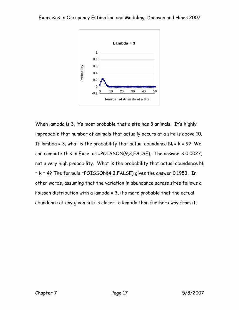
Here is another illustration of Poisson probabilities, this time for lambda = 3

and ranging over a set of possible site abundances (k) from 0 to 50.



Lambda = 3

-0.2

0

0.2

0.4

0.6

0.8

1

0 10 20 30 40 50

Number of Animals at a Site

Prob

abili

ty

When lambda is 3, it’s most probable that a site has 3 animals. It’s highly

improbable that number of animals that actually occurs at a site is above 10.

If lambda = 3, what is the probability that actual abundance Ni = k = 9? We

can compute this in Excel as =POISSON(9,3,FALSE). The answer is 0.0027,

not a very high probability. What is the probability that actual abundance Ni

= k = 4? The formula =POISSON(4,3,FALSE) gives the answer 0.1953. In

other words, assuming that the variation in abundance across sites follows a

Poisson distribution with a lambda = 3, it’s more probable that the actual

abundance at any given site is closer to lambda than further away from it.



Lambda = 3

0

0.2

0.4

0.6

0.8

1

0 10 20 30 40 50

number of animals at a site

prob

abili

ty

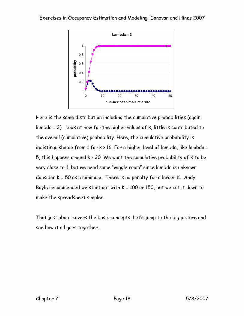
Here is the same distribution including the cumulative probabilities (again,

lambda = 3). Look at how for the higher values of k, little is contributed to

the overall (cumulative) probability. Here, the cumulative probability is

indistinguishable from 1 for k > 16. For a higher level of lambda, like lambda =

5, this happens around k > 20. We want the cumulative probability of K to be

very close to 1, but we need some “wiggle room” since lambda is unknown.

Consider K = 50 as a minimum. There is no penalty for a larger K. Andy

Royle recommended we start out with K = 100 or 150, but we cut it down to

make the spreadsheet simpler.

That just about covers the basic concepts. Let’s jump to the big picture and

see how it all goes together.



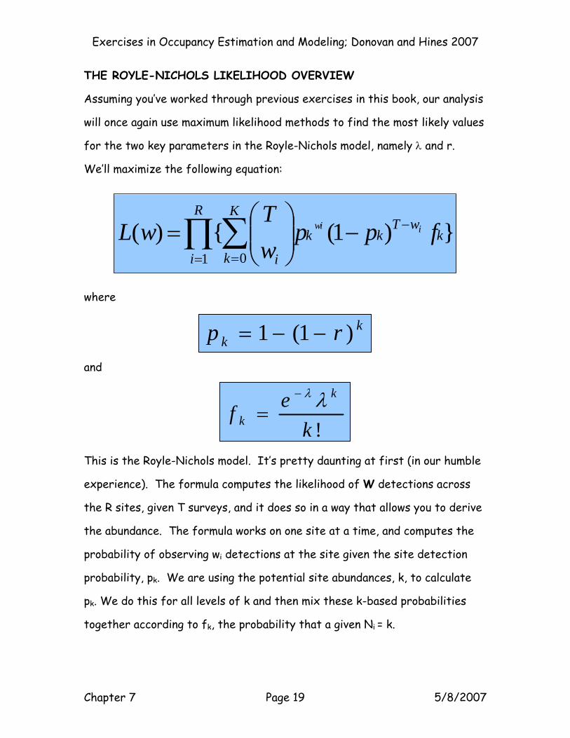
THE ROYLE-NICHOLS LIKELIHOOD OVERVIEW

Assuming you’ve worked through previous exercises in this book, our analysis

will once again use maximum likelihood methods to find the most likely values

for the two key parameters in the Royle-Nichols model, namely λ and r.

We’ll maximize the following equation:

where

and

This is the Royle-Nichols model. It’s pretty daunting at first (in our humble

experience). The formula computes the likelihood of W detections across

the R sites, given T surveys, and it does so in a way that allows you to derive

the abundance. The formula works on one site at a time, and computes the

probability of observing wi detections at the site given the site detection

probability, pk. We are using the potential site abundances, k, to calculate

pk. We do this for all levels of k and then mix these k-based probabilities

together according to fk, the probability that a given Ni = k.

})1({)(1 0∏ ∑=

−

=

−⎟⎟⎠

⎞⎜⎜⎝

⎛=

R

i

kwT

kk

K

k i

fppwT

wL iwi

kk rp )1(1 −−=

!kef

k

kλλ−

=



HERE WE GO!

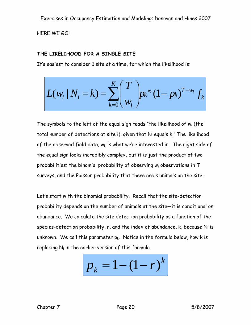
THE LIKELIHOOD FOR A SINGLE SITE

It’s easiest to consider 1 site at a time, for which the likelihood is:

The symbols to the left of the equal sign reads “the likelihood of wi (the

total number of detections at site i), given that Ni equals k.” The likelihood

of the observed field data, wi, is what we’re interested in. The right side of

the equal sign looks incredibly complex, but it is just the product of two

probabilities: the binomial probability of observing wi observations in T

surveys, and the Poisson probability that there are k animals on the site.

Let’s start with the binomial probability. Recall that the site-detection

probability depends on the number of animals at the site—it is conditional on

abundance. We calculate the site detection probability as a function of the

species-detection probability, r, and the index of abundance, k, because Ni is

unknown. We call this parameter pk. Notice in the formula below, how k is

replacing Ni in the earlier version of this formula.

kk rp )1(1 −−=

kwT

kk

K

k iii fpp

wT

kNwL iiw −

=

−⎟⎟⎠

⎞⎜⎜⎝

⎛== ∑ )1()|(

0



This function tells us the probability of seeing an animal at this site for a

given level of k. Our data are the sums of the number of detections over T

survey visits, wi. The results of a survey occasion are binomial, a 1 or a 0, so

detection at a site is a binomial probability. We want to find the probability

of observing wi detections over T surveys (in this case, 5), given the

probability of a success is pk. This is a binomial probability. A binomial

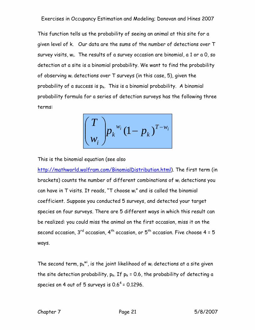
probability formula for a series of detection surveys has the following three

terms:

This is the binomial equation (see also

http://mathworld.wolfram.com/BinomialDistribution.html). The first term (in

brackets) counts the number of different combinations of wi detections you

can have in T visits. It reads, “T choose wi” and is called the binomial

coefficient. Suppose you conducted 5 surveys, and detected your target

species on four surveys. There are 5 different ways in which this result can

be realized: you could miss the animal on the first occasion, miss it on the

second occasion, 3rd occasion, 4th occasion, or 5th occasion. Five choose 4 = 5

ways.

The second term, pkwi, is the joint likelihood of wi detections at a site given

the site detection probability, pk. If pk = 0.6, the probability of detecting a

species on 4 out of 5 surveys is 0.64 = 0.1296.

ii wTk

wk

i

ppwT −−⎟⎟⎠

⎞⎜⎜⎝

⎛)1(



The final term, (1-pk)T-wi is the likelihood associated with the occasions when

nothing was detected. Failing to detect the target species at a site on a

given visit is 1 minus pk. Raising this to the power of T-wi gives the joint

probability of missing T-wi detections on each of the visits where you saw

nothing. If pk = 0.6, the probability of missing a species in 1 out of 5 surveys

is 0.41 = 0.4.

ii wTk

wk

i

ppwT −−⎟⎟⎠

⎞⎜⎜⎝

⎛)1(

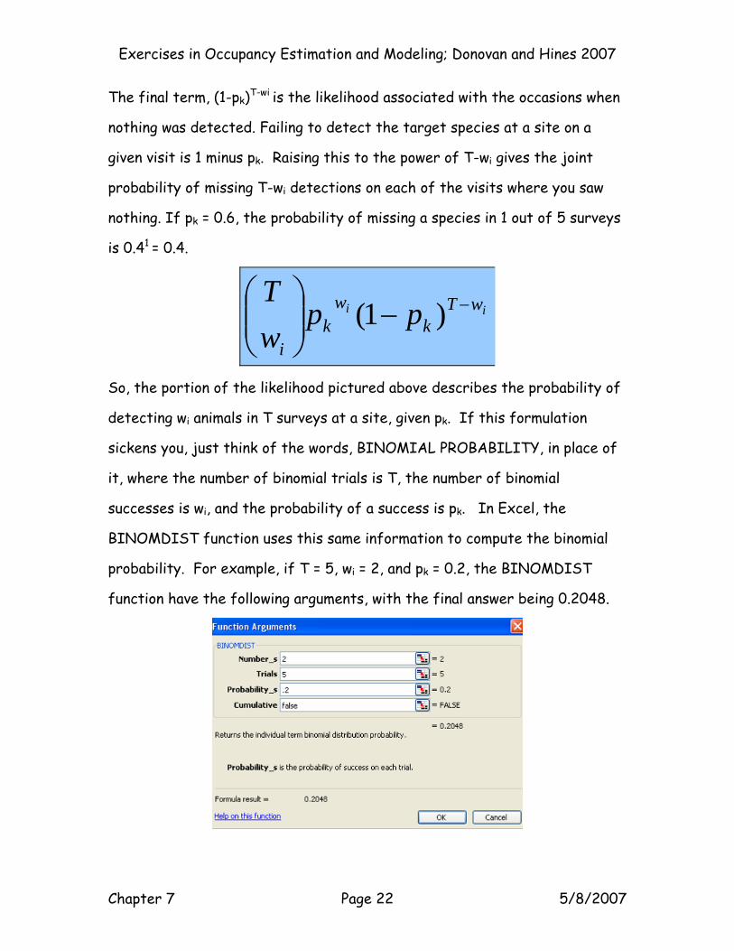
So, the portion of the likelihood pictured above describes the probability of

detecting wi animals in T surveys at a site, given pk. If this formulation

sickens you, just think of the words, BINOMIAL PROBABILITY, in place of

it, where the number of binomial trials is T, the number of binomial

successes is wi, and the probability of a success is pk. In Excel, the

BINOMDIST function uses this same information to compute the binomial

probability. For example, if T = 5, wi = 2, and pk = 0.2, the BINOMDIST

function have the following arguments, with the final answer being 0.2048.



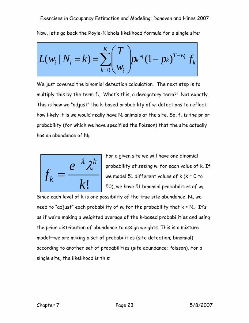
Now, let’s go back the Royle-Nichols likelihood formula for a single site:

We just covered the binomial detection calculation. The next step is to

multiply this by the term fk. What’s this, a derogatory term?! Not exactly.

This is how we “adjust” the k-based probability of wi detections to reflect

how likely it is we would really have Ni animals at the site. So, fk is the prior

probability (for which we have specified the Poisson) that the site actually

has an abundance of Ni.

For a given site we will have one binomial

probability of seeing wi for each value of k. If

we model 51 different values of k (k = 0 to

50), we have 51 binomial probabilities of wi.

Since each level of k is one possibility of the true site abundance, Ni, we

need to “adjust” each probability of wi for the probability that k = Ni. It’s

as if we’re making a weighted average of the k-based probabilities and using

the prior distribution of abundance to assign weights. This is a mixture

model—we are mixing a set of probabilities (site detection; binomial)

according to another set of probabilities (site abundance; Poisson). For a

single site, the likelihood is this:

!kef

k

kλλ−

=

kwT

kk

K

k iii fpp

wT

kNwL iiw −

=

−⎟⎟⎠

⎞⎜⎜⎝

⎛== ∑ )1()|(

0



You should recognize the binomial probability of wi based on pk. The fk term

is the mixing probability—here, the Poisson prior distribution that k = Ni.

The summation symbol tells us to mix all these together for the whole range

of k for the wi of this site. Is this making sense?

THE ROYLE-NICHOLS LIKELIHOOD FOR ALL SITES

The next step is to combine the site-likelihoods to get the likelihood over

the whole survey (R sites):

The big Π is telling you to take the product of the terms to the right for

each site i from i = 1 to R. This is the product of all of the likelihoods for

each site. This product is the likelihood of seeing this collection of wi values

for the whole survey area.

Since we are using the Poisson distribution of k to stand in for Ni, we now

need to estimate lambda for this distribution. Ni has been removed from the

})1({)(1 0∏ ∑=

−

=

−⎟⎟⎠

⎞⎜⎜⎝

⎛=

R

i

kwT

kk

K

k i

fppwT

wL iwi

kwT

kk

K

k iii fpp

wT

kNwL iiw −

=

−⎟⎟⎠

⎞⎜⎜⎝

⎛== ∑ )1()|(

0



formula. If we can estimate r and lambda from the data, we can then derive

N. We will use Excel to find those combinations of r and lambda that

maximize the overall likelihood. That’s why you didn’t need to worry about

the “given r” and “given lambda” stuff before. Excel will just plug in values

for these parameters and then tell us the values for each that maximize the

overall likelihood.

That’s it! Once you estimate r and lambda, you can calculate an estimate of N

(study area abundance) and psi (the probability of occupancy). Let’s go to

the spreadsheets and see it work.

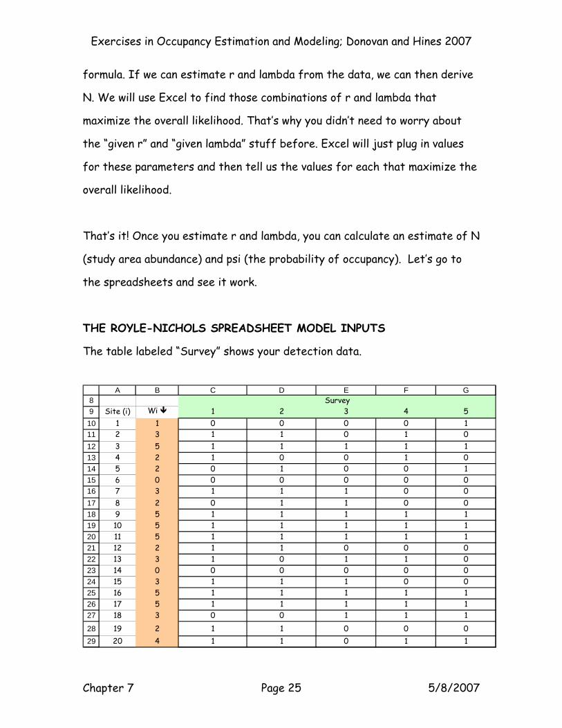
THE ROYLE-NICHOLS SPREADSHEET MODEL INPUTS

The table labeled “Survey” shows your detection data.

89

101112131415161718192021222324252627

2829

A B C D E F G

Site (i) Wi 1 2 3 4 51 1 0 0 0 0 12 3 1 1 0 1 03 5 1 1 1 1 14 2 1 0 0 1 05 2 0 1 0 0 16 0 0 0 0 0 07 3 1 1 1 0 08 2 0 1 1 0 09 5 1 1 1 1 110 5 1 1 1 1 111 5 1 1 1 1 112 2 1 1 0 0 013 3 1 0 1 1 014 0 0 0 0 0 015 3 1 1 1 0 016 5 1 1 1 1 117 5 1 1 1 1 118 3 0 0 1 1 119 2 1 1 0 0 020 4 1 1 0 1 1

Survey



Above is a picture of results from all 20 sites. The 20 sites are listed in the

column on the left and the 5 periods run left to right. The first site had one

detection, which occurred in the last survey (00001). The second site had

detections in periods 1, 2, and 4 only. In the column “Wi” (B10:B29) are the

total detections, wi, for each site. Believe it or not, that’s basically it in

terms of data entry.

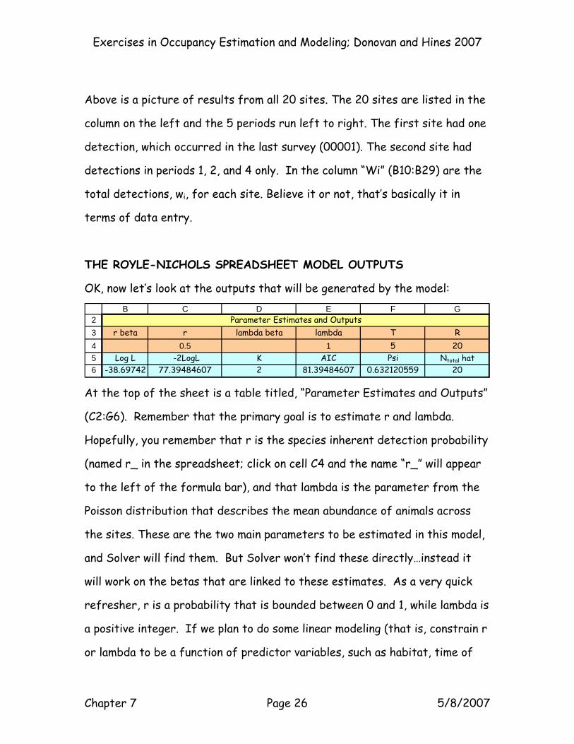
THE ROYLE-NICHOLS SPREADSHEET MODEL OUTPUTS

OK, now let’s look at the outputs that will be generated by the model:

23456

B C D E F G

r beta r lambda beta lambda T R0.5 1 5 20

Log L -2LogL K AIC Psi Ntotal hat-38.69742 77.39484607 2 81.39484607 0.632120559 20

Parameter Estimates and Outputs

At the top of the sheet is a table titled, “Parameter Estimates and Outputs”

(C2:G6). Remember that the primary goal is to estimate r and lambda.

Hopefully, you remember that r is the species inherent detection probability

(named r_ in the spreadsheet; click on cell C4 and the name “r_” will appear

to the left of the formula bar), and that lambda is the parameter from the

Poisson distribution that describes the mean abundance of animals across

the sites. These are the two main parameters to be estimated in this model,

and Solver will find them. But Solver won’t find these directly…instead it

will work on the betas that are linked to these estimates. As a very quick

refresher, r is a probability that is bounded between 0 and 1, while lambda is

a positive integer. If we plan to do some linear modeling (that is, constrain r

or lambda to be a function of predictor variables, such as habitat, time of



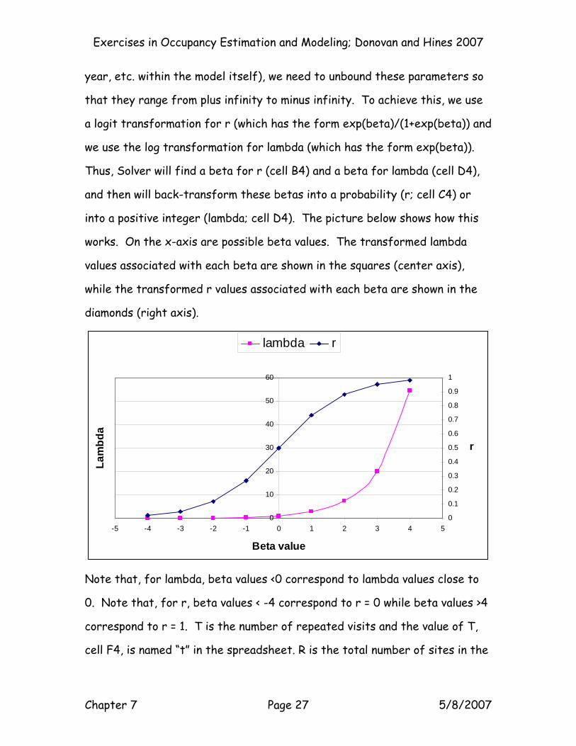
year, etc. within the model itself), we need to unbound these parameters so

that they range from plus infinity to minus infinity. To achieve this, we use

a logit transformation for r (which has the form exp(beta)/(1+exp(beta)) and

we use the log transformation for lambda (which has the form exp(beta)).

Thus, Solver will find a beta for r (cell B4) and a beta for lambda (cell D4),

and then will back-transform these betas into a probability (r; cell C4) or

into a positive integer (lambda; cell D4). The picture below shows how this

works. On the x-axis are possible beta values. The transformed lambda

values associated with each beta are shown in the squares (center axis),

while the transformed r values associated with each beta are shown in the

diamonds (right axis).

0

10

20

30

40

50

60

-5 -4 -3 -2 -1 0 1 2 3 4 5

Beta value

Lam

bda

0

0.1

0.2

0.3

0.4

0.5

0.6

0.7

0.8

0.9

1

r

lambda r

Note that, for lambda, beta values <0 correspond to lambda values close to

0. Note that, for r, beta values < -4 correspond to r = 0 while beta values >4

correspond to r = 1. T is the number of repeated visits and the value of T,

cell F4, is named “t” in the spreadsheet. R is the total number of sites in the



survey and is named _R in the spreadsheet (cell G4). The primary outputs of

the model are given in the blue-shaded cells. In cell B6 is the Log Likelihood.

This is the log of the total likelihood for all sites combined. We will estimate

r and lambda by maximizing this cell. In cell C6 is the -2*Log Likelihood. K

(cell D6) is the number of parameters being estimated (namely, r and λ) and

is also used in calculating AIC. AIC is calculated in cell E6 as -2LogeL + 2K.

Psi (cell F6) is the probability of occupancy for a given site. It is derived

from the Poisson function for the given lambda—the probability that a site

is occupied is 1 minus the Poisson probability that the abundance is 0. N-hat

is the estimated total abundance (cell G6). N-hat is derived, and is

estimated as lambda*R, the mean site abundance times the number of sites.

We’ll revisit these outputs soon.

THE LIKELIHOOD FOR SITES, ONE AT A TIME

OK, now let’s get to the analytical meat of the spreadsheet.

31323334353637

A B C D E F G Hk => 0 1 2 3 4 5pk => 0.000000 0.399812 0.639774 0.783796 0.870237 0.922118

1 1 0.00000 0.05911 0.01424 0.00175 0.00015 0.000012 3 0.00000 0.05246 0.08986 0.04605 0.01317 0.002623 5 0.00000 0.00233 0.02834 0.06052 0.05924 0.036734 2 0.00000 0.07876 0.05060 0.01270 0.00196 0.000225 2 0.00000 0.07876 0.05060 0.01270 0.00196 0.00022

The table, “Likelihood wi” (A30:BC53), is where we calculate the likelihood of

our data, given r and lambda. In this spreadsheet, k ranges from 0 to 50

(row 31, green cells), so we are considering a mixture of 51 possible

abundance values, k. For any given k, the site detection probability pk is

computed in row 32 with the formula =1-(1-r_)^k. Click on cell C32 and you

should see the formula =1-(1-r_)^C31. Excel returns a 0 here because 1-(any



number raised to the 0) is 0. This is good because if k = 0, the actual

abundance is 0 and so the probability of detecting any animals should be 0.

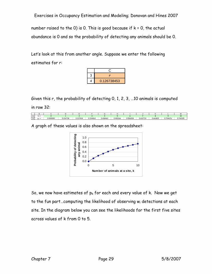
Let’s look at this from another angle. Suppose we enter the following

estimates for r:

34

Cr

0.126738453

Given this r, the probability of detecting 0, 1, 2, 3, …10 animals is computed

in row 32:

3132

B C D E F G H I J K L Mk => 0 1 2 3 4 5 6 7 8 9 10pk => 0.000000 0.126738 0.237414 0.334063 0.418463 0.492166 0.556528 0.612733 0.661815 0.704676 0.742105

A graph of these values is also shown on the spreadsheet:

0.00.20.4

0.60.81.0

0 5 10

Number of animals at a site, k

Prob

abili

ty o

f det

ectin

g an

y an

imal

So, we now have estimates of pk for each and every value of k. Now we get

to the fun part…computing the likelihood of observing wi detections at each

site. In the diagram below you can see the likelihoods for the first five sites

across values of k from 0 to 5.



31323334353637

B C D E F G Hk => 0 1 2 3 4 5pk => 0.000000 0.126738 0.237414 0.334063 0.418463 0.492166

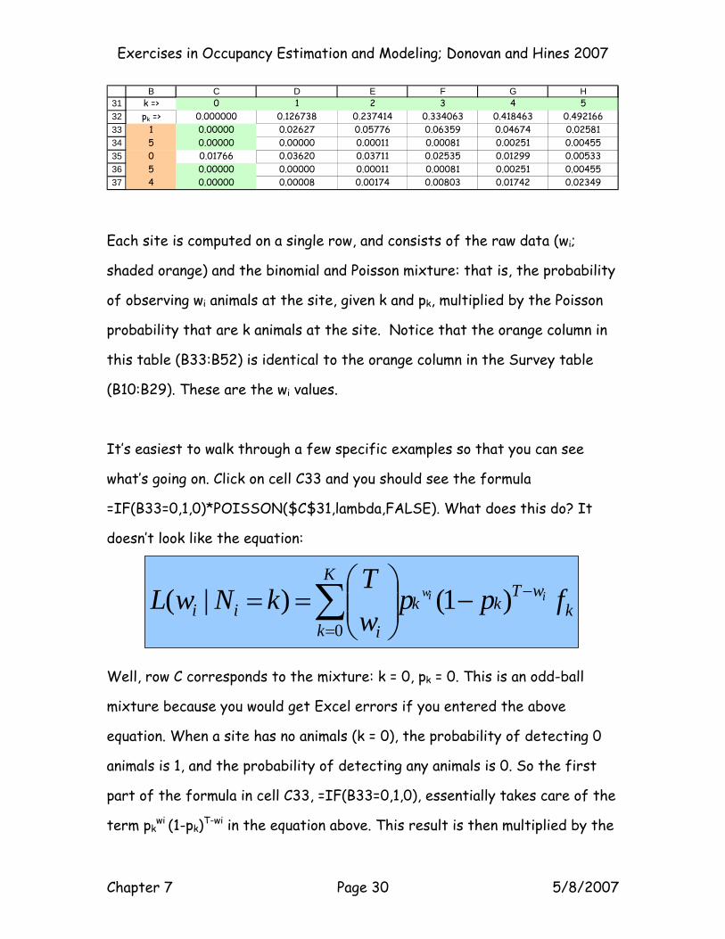
1 0.00000 0.02627 0.05776 0.06359 0.04674 0.025815 0.00000 0.00000 0.00011 0.00081 0.00251 0.004550 0.01766 0.03620 0.03711 0.02535 0.01299 0.005335 0.00000 0.00000 0.00011 0.00081 0.00251 0.004554 0.00000 0.00008 0.00174 0.00803 0.01742 0.02349

Each site is computed on a single row, and consists of the raw data (wi;

shaded orange) and the binomial and Poisson mixture: that is, the probability

of observing wi animals at the site, given k and pk, multiplied by the Poisson

probability that are k animals at the site. Notice that the orange column in

this table (B33:B52) is identical to the orange column in the Survey table

(B10:B29). These are the wi values.

It’s easiest to walk through a few specific examples so that you can see

what’s going on. Click on cell C33 and you should see the formula

=IF(B33=0,1,0)*POISSON($C$31,lambda,FALSE). What does this do? It

doesn’t look like the equation:

Well, row C corresponds to the mixture: k = 0, pk = 0. This is an odd-ball

mixture because you would get Excel errors if you entered the above

equation. When a site has no animals (k = 0), the probability of detecting 0

animals is 1, and the probability of detecting any animals is 0. So the first

part of the formula in cell C33, =IF(B33=0,1,0), essentially takes care of the

term pkwi (1-pk)T-wi in the equation above. This result is then multiplied by the

kwT

kk

K

k iii fpp

wT

kNwL iiw −

=

−⎟⎟⎠

⎞⎜⎜⎝

⎛== ∑ )1()|(

0



term POISSON($C$31,lambda,FALSE), which is the probability that 0

animals occur at a site, given lambda. That does it for the first mixture,

where k = 0. This part wasn’t obvious at first but with Andy Royle’s generous

help and some attitude adjustment from the Program PRESENCE help files,

we were able to get this part of the model to work.

Now let’s look at the next mixture for site 1: k = 1. Click on cell D33 and you

should see the formula:

=BINOMDIST($B33,t,D$32,FALSE)*POISSON(D$31,lambda,FALSE),

which describes the right hand side of the likelihood function:

This is the probability mixture for k = 1…..it is a binomial probability (in red

type) multiplied by a Poisson probability (in blue type). When k = 1, we first

compute pk as 1-(1-r)^1 (cell D32). Knowing k and pk for this mixture, we now

compute binomial probability of detecting wi animals at site 1 with the

binomial equation BINOMDIST($B33,t,D$32,FALSE), and then multiply this

by the probability that the actual abundance at site 1 was really 1, given



lambda POISSON(D$31,lambda,FALSE). Make sense? This formula is copied

across for the other 49 mixtures for that site. The site likelihood for site 1

is computed in cell BB33 by adding the 51 k-based results together. If

you’ve done the CJS models, the result is analogous to an encounter history

probability for the site. Cell BC33 is the natural log of the site likelihood.

Taking the natural log of a likelihood is a common practice to simplify

calculations.

We then repeat this process for the other sites. So the likelihood equation

for each site consists of 51 entries that are added together, and this

happens for all 20 (R = 20) sites.

The end result is the likelihood and log likelihood for each of the 20 sites:

kwT

kk

K

k iii fpp

wT

kNwL iiw −

=

−⎟⎟⎠

⎞⎜⎜⎝

⎛== ∑ )1()|(

0



3233343536373839404142

4344454647484950515253

A B BB BCpk => site likelihood ln(site likelihood)

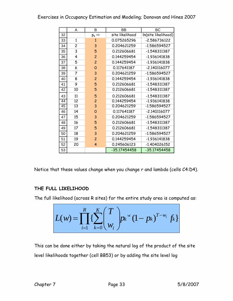
1 1 0.075265296 -2.5867361222 3 0.204621259 -1.5865945273 5 0.212606681 -1.5483113874 2 0.144259454 -1.9361418385 2 0.144259454 -1.9361418386 0 0.117641187 -2.1401160777 3 0.204621259 -1.5865945278 2 0.144259454 -1.9361418389 5 0.212606681 -1.54831138710 5 0.212606681 -1.54831138711 5 0.212606681 -1.54831138712 2 0.144259454 -1.93614183813 3 0.204621259 -1.58659452714 0 0.117641187 -2.14011607715 3 0.204621259 -1.58659452716 5 0.212606681 -1.54831138717 5 0.212606681 -1.54831138718 3 0.204621259 -1.58659452719 2 0.144259454 -1.93614183820 4 0.245606123 -1.404026152

-35.17454458 -35.17454458

Notice that these values change when you change r and lambda (cells C4:D4).

THE FULL LIKELIHOOD

The full likelihood (across R sites) for the entire study area is computed as:

This can be done either by taking the natural log of the product of the site

level likelihoods together (cell BB53) or by adding the site level log

})1({)(1 0∏ ∑=

−

=

−⎟⎟⎠

⎞⎜⎜⎝

⎛=

R

i

kwT

kk

K

k i

fppwT

wL iwi



likelihoods together (cell BC53). We will maximize the log likelihood to

estimate the parameters, r and λ, for our data across all sites.

Look carefully at the likelihoods (BB33:BB52) and notice that some are equal

to others. Seeing that the site likelihoods are the same for these two sites

tells us what? It tells us that they have the same wi. All of the other

parameters and variables are the same for calculating the likelihoods of the

sites. Differences in the site likelihoods are caused by differences in wi

RUNNING THE MODEL

The spreadsheet is set up to estimate r and lambda from the raw data in the

Survey table (cells C10:G29). To do this, you run the Excel function, Solver,

which we’ll do in a moment. Solver will find the maximum log Likelihood by

changing the values of r and lambda.

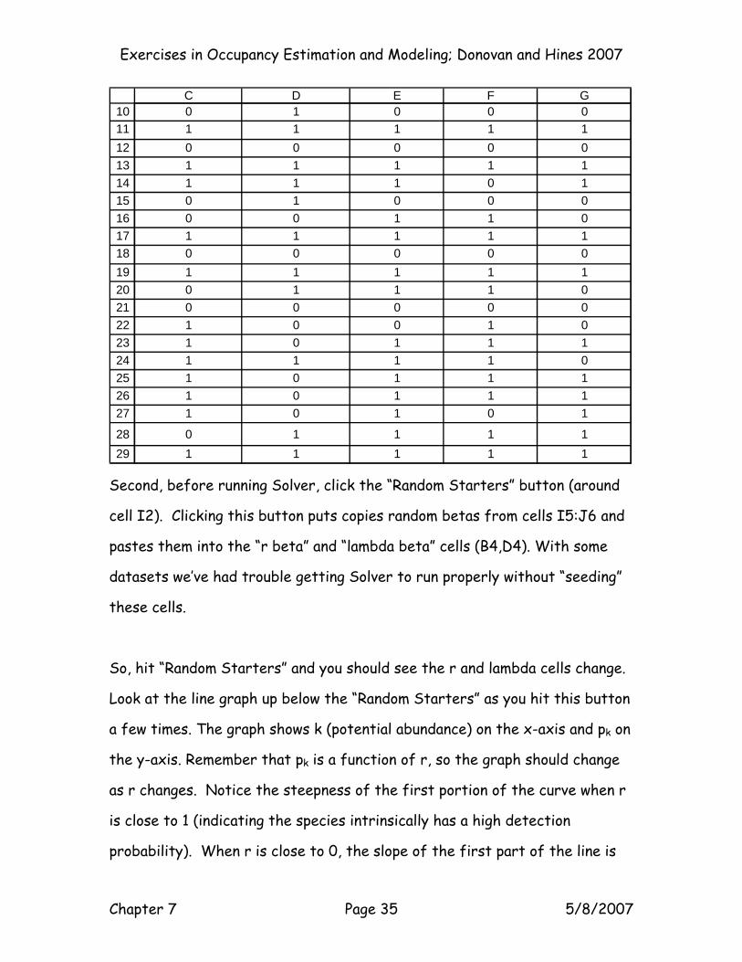
Before we begin, do two things. First, make sure the inputs on your

spreadsheet match those shown below:



101112131415161718192021222324252627

2829

C D E F G0 1 0 0 01 1 1 1 10 0 0 0 01 1 1 1 11 1 1 0 10 1 0 0 00 0 1 1 01 1 1 1 10 0 0 0 01 1 1 1 10 1 1 1 00 0 0 0 01 0 0 1 01 0 1 1 11 1 1 1 01 0 1 1 11 0 1 1 11 0 1 0 1

0 1 1 1 11 1 1 1 1

Second, before running Solver, click the “Random Starters” button (around

cell I2). Clicking this button puts copies random betas from cells I5:J6 and

pastes them into the “r beta” and “lambda beta” cells (B4,D4). With some

datasets we’ve had trouble getting Solver to run properly without “seeding”

these cells.

So, hit “Random Starters” and you should see the r and lambda cells change.

Look at the line graph up below the “Random Starters” as you hit this button

a few times. The graph shows k (potential abundance) on the x-axis and pk on

the y-axis. Remember that pk is a function of r, so the graph should change

as r changes. Notice the steepness of the first portion of the curve when r

is close to 1 (indicating the species intrinsically has a high detection

probability). When r is close to 0, the slope of the first part of the line is



very flat. In this case, the species is intrinsically difficult to detect, and

there must be a lot of animals present at the site for site detection

probability to be somewhat reasonable. For now, we are just looking at

random betas and their associated r and lambda estimates…these are not

the maximized estimates. Once we have our maximized estimates, though,

we will refer back to this graph.

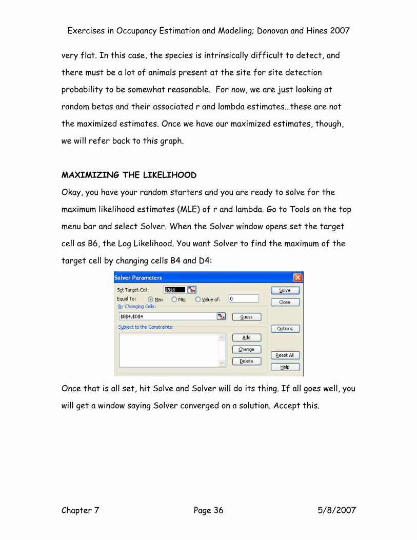
MAXIMIZING THE LIKELIHOOD

Okay, you have your random starters and you are ready to solve for the

maximum likelihood estimates (MLE) of r and lambda. Go to Tools on the top

menu bar and select Solver. When the Solver window opens set the target

cell as B6, the Log Likelihood. You want Solver to find the maximum of the

target cell by changing cells B4 and D4:

Once that is all set, hit Solve and Solver will do its thing. If all goes well, you

will get a window saying Solver converged on a solution. Accept this.



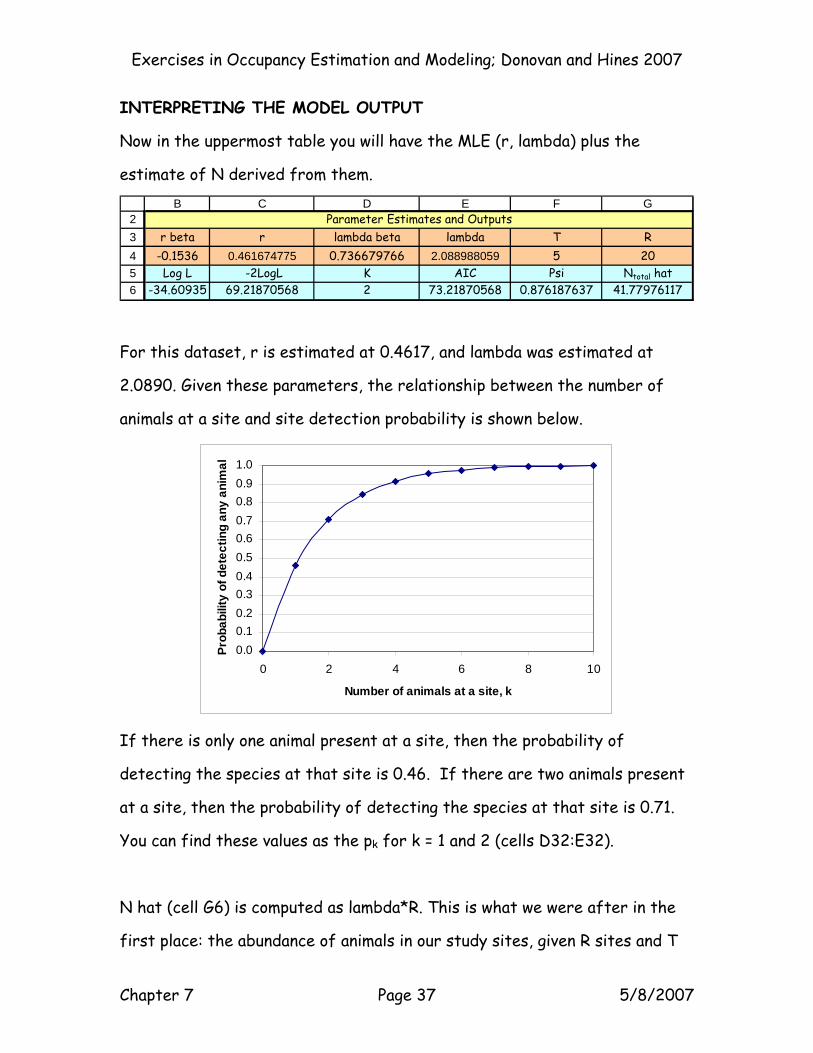
INTERPRETING THE MODEL OUTPUT

Now in the uppermost table you will have the MLE (r, lambda) plus the

estimate of N derived from them.

23456

B C D E F G

r beta r lambda beta lambda T R-0.1536 0.461674775 0.736679766 2.088988059 5 20Log L -2LogL K AIC Psi Ntotal hat

-34.60935 69.21870568 2 73.21870568 0.876187637 41.77976117


For this dataset, r is estimated at 0.4617, and lambda was estimated at

2.0890. Given these parameters, the relationship between the number of

animals at a site and site detection probability is shown below.

0.00.10.20.30.40.50.60.70.80.91.0

0 2 4 6 8 10

Number of animals at a site, k

Prob

abili

ty o

f det

ectin

g an

y an

imal

If there is only one animal present at a site, then the probability of

detecting the species at that site is 0.46. If there are two animals present

at a site, then the probability of detecting the species at that site is 0.71.

You can find these values as the pk for k = 1 and 2 (cells D32:E32).

N hat (cell G6) is computed as lambda*R. This is what we were after in the

first place: the abundance of animals in our study sites, given R sites and T



surveys. AIC is computed as -2LogeL *2*the number of parameters

estimated in the model. In this model, there are two estimated parameters,

r and lambda. Psi is the probability that a site is occupied. Now that we know

lambda = 2.0890, we can compute the probability of getting 0 animals as

POISSON(0,2.0890,FALSE), and 1 minus this is the probability of not

getting a 0 (Psi). Those are the basic outputs in PRESENCE. We’ll run this in

PRESENCE soon.

SIMULATING DATA

Before going on to PRESENCE, let’s look at how the raw data are simulated.

It quite simply takes the model and turns it inside out to generate the

survey results. First a Poisson distribution is used to generate Ni for each

site. Then you “flip a coin” a number of times for each visit to each site to

see if any animals were detected.

Open the Simulate Data sheet. You can see the Poisson distribution function

set up along the left side of the sheet in columns A:C.



234567891011121314151617

A B CLambda 2r = 0.95

Prob Mass Prob DensityNi 00 0.135335283 0.1353352831 0.270670566 0.406005852 0.270670566 0.6766764163 0.180447044 0.857123464 0.090223522 0.9473469835 0.036089409 0.9834363926 0.012029803 0.9954661947 0.003437087 0.9989032818 0.000859272 0.9997625539 0.000190949 0.99995350210 3.81899E-05 0.999991692

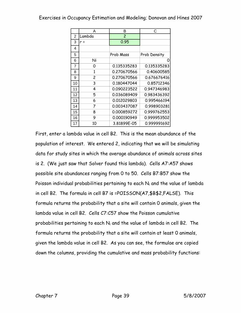
First, enter a lambda value in cell B2. This is the mean abundance of the

population of interest. We entered 2, indicating that we will be simulating

data for study sites in which the average abundance of animals across sites

is 2. (We just saw that Solver found this lambda). Cells A7:A57 shows

possible site abundances ranging from 0 to 50. Cells B7:B57 show the

Poisson individual probabilities pertaining to each Ni and the value of lambda

in cell B2. The formula in cell B7 is =POISSON(A7,$B$2,FALSE). This

formula returns the probability that a site will contain 0 animals, given the

lambda value in cell B2. Cells C7:C57 show the Poisson cumulative

probabilities pertaining to each Ni and the value of lambda in cell B2. The

formula returns the probability that a site will contain at least 0 animals,

given the lambda value in cell B2. As you can see, the formulae are copied

down the columns, providing the cumulative and mass probability functions:



Lambda

0

0.2

0.4

0.6

0.8

1

0 2 4 6 8 10Number of Animals at a Site

Prob

abili

ty

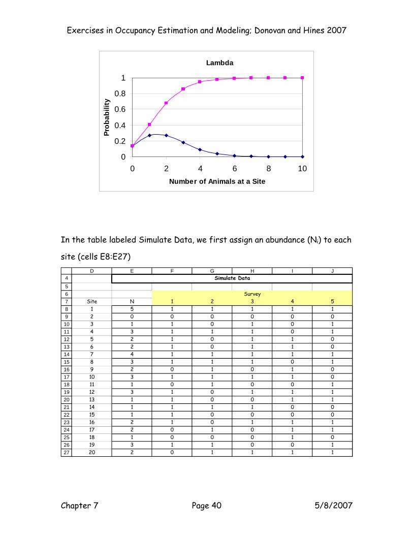
In the table labeled Simulate Data, we first assign an abundance (Ni) to each

site (cells E8:E27)

456789

101112131415161718192021222324252627

D E F G H I J

Site N 1 2 3 4 51 5 1 1 1 1 12 0 0 0 0 0 03 1 1 0 1 0 14 3 1 1 1 0 15 2 1 0 1 1 06 2 1 0 1 1 07 4 1 1 1 1 18 3 1 1 1 0 19 2 0 1 0 1 010 3 1 1 1 1 011 1 0 1 0 0 112 3 1 0 1 1 113 1 1 0 0 1 114 1 1 1 1 0 015 1 1 0 0 0 016 2 1 0 1 1 117 2 0 1 0 1 118 1 0 0 0 1 019 3 1 1 0 0 120 2 0 1 1 1 1

Simulate Data

Survey



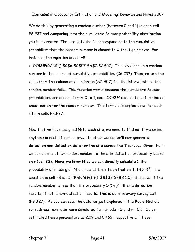
We do this by generating a random number (between 0 and 1) in each cell

E8:E27 and comparing it to the cumulative Poisson probability distribution

you just created. The site gets the Ni corresponding to the cumulative

probability that the random number is closest to without going over. For

instance, the equation in cell E8 is

=LOOKUP(RAND(),$C$6:$C$57,$A$7:$A$57). This says look up a random

number in the column of cumulative probabilities (C6:C57). Then, return the

value from the column of abundances (A7:A57) for the interval where the

random number falls. This function works because the cumulative Poisson

probabilities are ordered from 0 to 1, and LOOKUP does not need to find an

exact match for the random number. This formula is copied down for each

site in cells E8:E27.

Now that we have assigned Ni to each site, we need to find out if we detect

anything in each of our surveys. In other words, we’ll now generate

detection non-detection data for the site across the T surveys. Given the Ni,

we compare another random number to the site detection probability based

on r (cell B3). Here, we know Ni so we can directly calculate 1-the

probability of missing all Ni animals at the site on that visit, 1-(1-r)Ni. The

equation in cell F8 is =IF(RAND()<(1-((1-$B$3)^$E8)),1,0). This says: if the

random number is less than the probability 1-(1-r)Ni, then a detection

results, if not, a non-detection results. This is done in every survey cell

(F8:J27). As you can see, the data we just explored in the Royle-Nichols

spreadsheet exercise were simulated for lambda = 2 and r = 0.5. Solver

estimated these parameters as 2.09 and 0.462, respectively. These



estimates may or may not be biased because the data were, after all,

simulated with stochasticity.

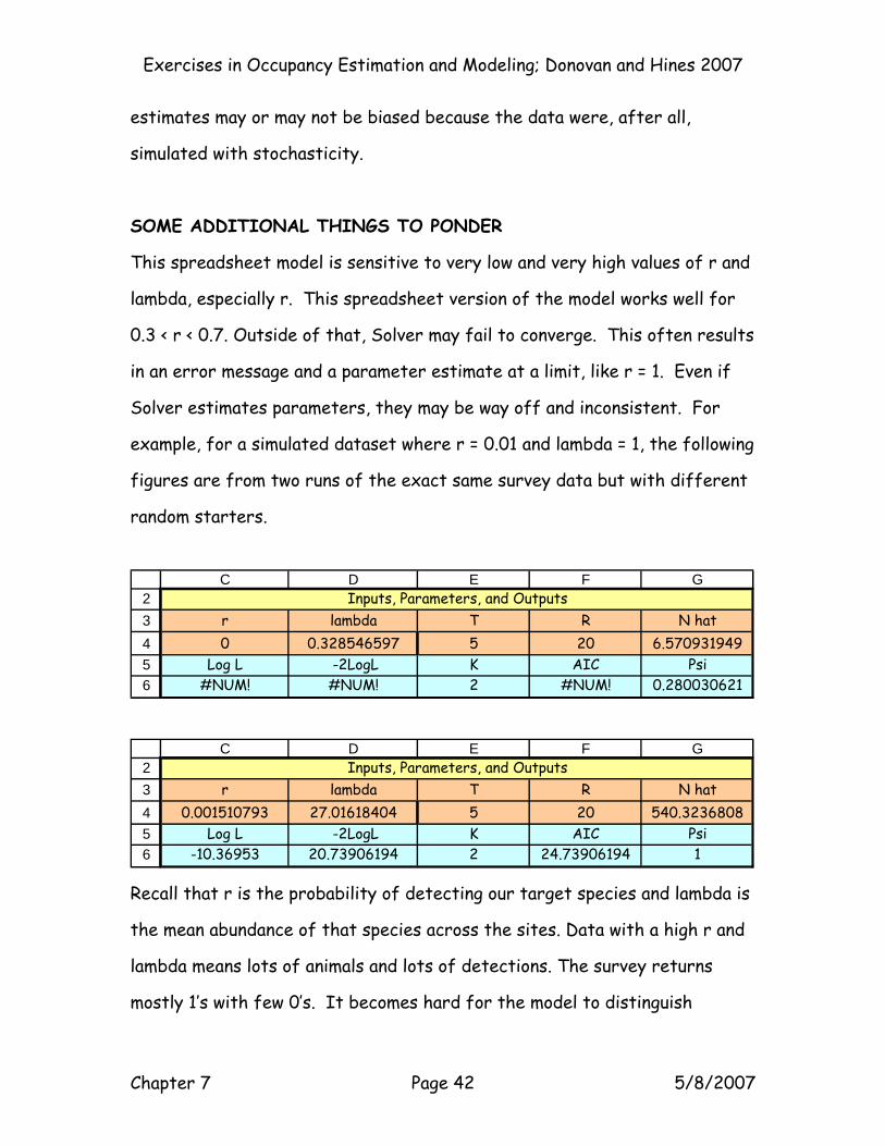
SOME ADDITIONAL THINGS TO PONDER

This spreadsheet model is sensitive to very low and very high values of r and

lambda, especially r. This spreadsheet version of the model works well for

0.3 < r < 0.7. Outside of that, Solver may fail to converge. This often results

in an error message and a parameter estimate at a limit, like r = 1. Even if

Solver estimates parameters, they may be way off and inconsistent. For

example, for a simulated dataset where r = 0.01 and lambda = 1, the following

figures are from two runs of the exact same survey data but with different

random starters.

23456

C D E F G

r lambda T R N hat0 0.328546597 5 20 6.570931949

Log L -2LogL K AIC Psi#NUM! #NUM! 2 #NUM! 0.280030621

Inputs, Parameters, and Outputs

23456

C D E F G

r lambda T R N hat0.001510793 27.01618404 5 20 540.3236808

Log L -2LogL K AIC Psi-10.36953 20.73906194 2 24.73906194 1

Inputs, Parameters, and Outputs

Recall that r is the probability of detecting our target species and lambda is

the mean abundance of that species across the sites. Data with a high r and

lambda means lots of animals and lots of detections. The survey returns

mostly 1’s with few 0’s. It becomes hard for the model to distinguish



whether r or lambda is driving the pattern. Conversely, data with low r and

low lambda result in surveys with mostly 0’s. There is nothing for the model

to work with here, so it fails to estimate parameters.

For more moderate, but slightly high and low, values of r, such as 0.8 and

0.3, you sometimes get estimates with Solver and other times you can’t. The

difference is how close the random seed is to the true value when you fire

up Solver. Recall from Exercise 1 that a likelihood surface can be a complex

surface and we are looking for the very top of this surface. The parameter

values associated with the peak of the surface are the maximum likelihood

estimates, telling us the best estimated values of the parameters. Solver

alters the parameter estimates and monitors the resulting likelihood (or log-

likelihood if you prefer). It “watches” the likelihood increase for changing

values of the parameters and when the likelihood starts to decrease, Solver

knows it has found the maximum likelihood. In many cases, there is a single

maximum peak on the likelihood surface, and Solver can find it. But in other

situations the likelihood surface has lots of little bumps and wiggles which

are local maxima and minima, fine-scale highs and lows. The highest point

over the whole profile is called the global maximum. In our case, unless the

random seed is near the global maximum, Solver will stop when it finds any

maximum—it doesn’t know to look for the global one. So it stops when it

finds whichever maximum is closest to where it began searching, the random

starter. This will return poor estimates since they don’t necessarily

maximize the likelihood overall.



The instability in our estimates is not completely inherent in the

spreadsheet model. One of the limitations here is the size of the survey.

We could improve this spreadsheet version by adding more sites, but the

improvement is not perfect. Royle and Nichols (2003) describe r > 0.15 as

the lower limit for good estimation with this model, even when simulating a

large number of sites (R = 100).



ROYLE-NICHOLS ABUNDANCE INDUCED HETEROGENEITY ANALYSIS IN PROGRAM PRESENCE

Hopefully you’ve worked through the spreadsheet Royle-Nichols Model by

now. If you haven’t done so, complete the spreadsheet exercise now.

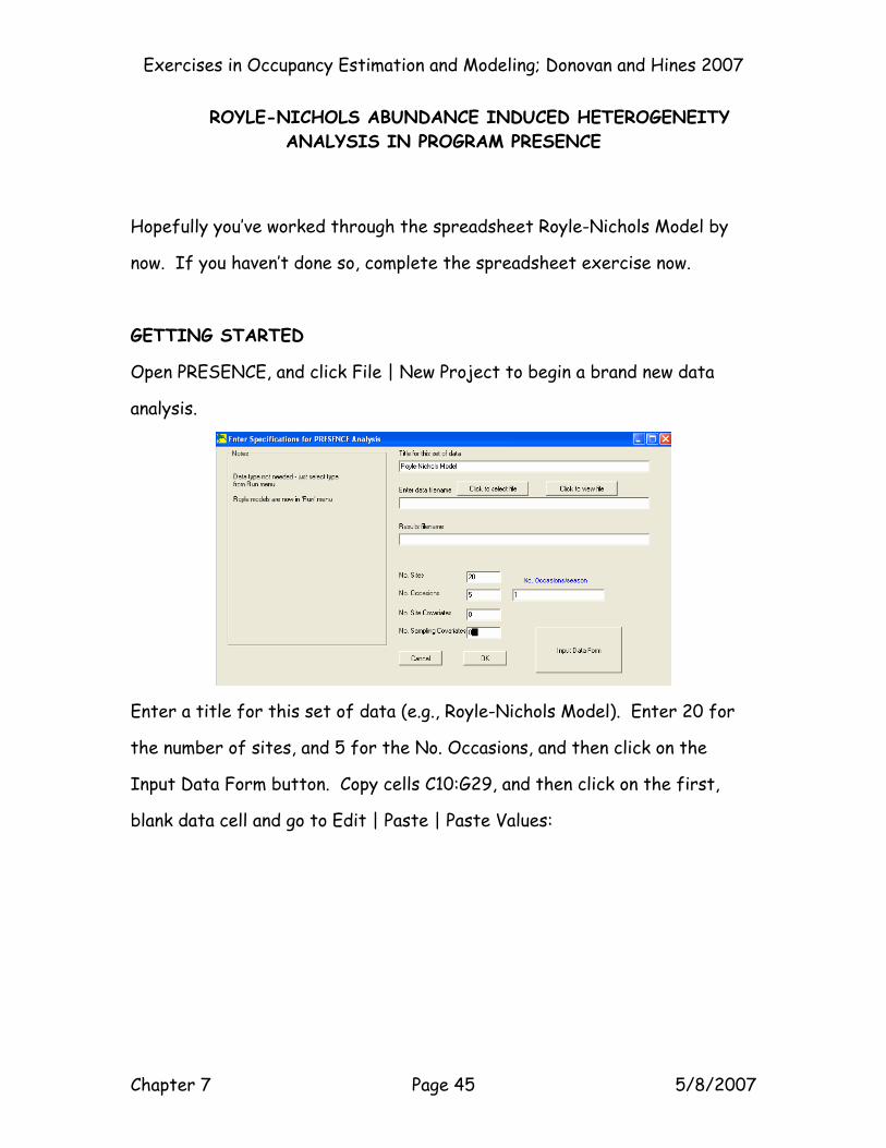
GETTING STARTED

Open PRESENCE, and click File | New Project to begin a brand new data

analysis.

Enter a title for this set of data (e.g., Royle-Nichols Model). Enter 20 for

the number of sites, and 5 for the No. Occasions, and then click on the

Input Data Form button. Copy cells C10:G29, and then click on the first,

blank data cell and go to Edit | Paste | Paste Values:



Then go to File | Save As and enter a file name for your new PRESENCE

input file, and store it somewhere where you can retrieve it easily:

Now, return to the Enter Specifications form, click the button labeled “Click

to Select File” and browse to your freshly created input file:



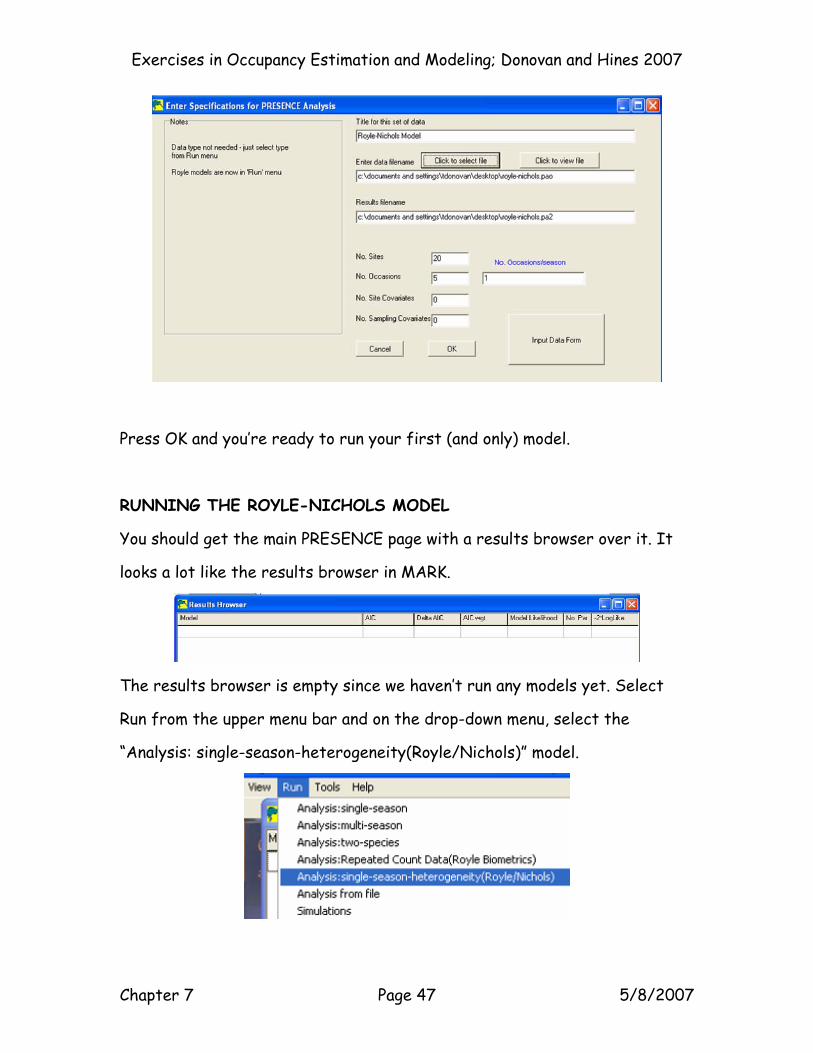
Press OK and you’re ready to run your first (and only) model.

RUNNING THE ROYLE-NICHOLS MODEL

You should get the main PRESENCE page with a results browser over it. It

looks a lot like the results browser in MARK.

The results browser is empty since we haven’t run any models yet. Select

Run from the upper menu bar and on the drop-down menu, select the

“Analysis: single-season-heterogeneity(Royle/Nichols)” model.



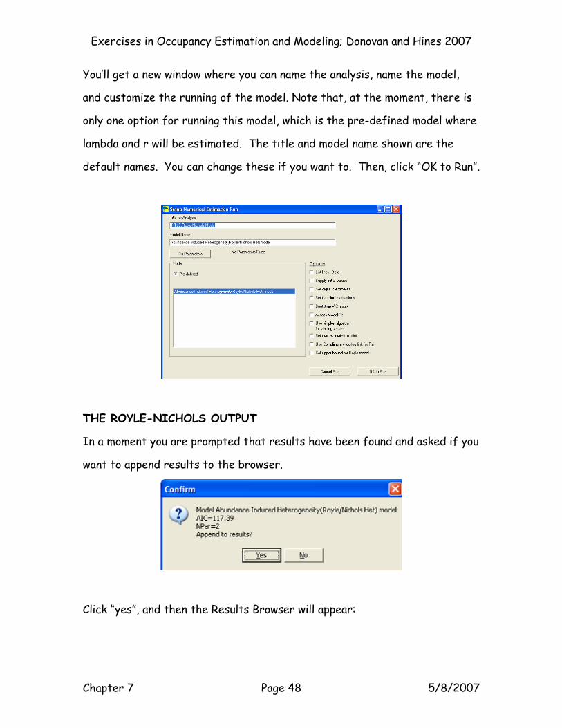
You’ll get a new window where you can name the analysis, name the model,

and customize the running of the model. Note that, at the moment, there is

only one option for running this model, which is the pre-defined model where

lambda and r will be estimated. The title and model name shown are the

default names. You can change these if you want to. Then, click “OK to Run”.

THE ROYLE-NICHOLS OUTPUT

In a moment you are prompted that results have been found and asked if you

want to append results to the browser.

Click “yes”, and then the Results Browser will appear:



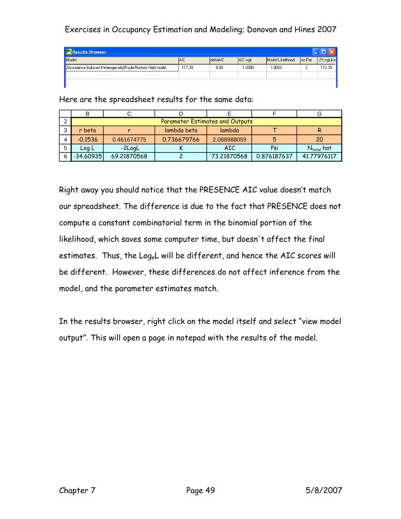
Here are the spreadsheet results for the same data:

23456

B C D E F G

r beta r lambda beta lambda T R-0.1536 0.461674775 0.736679766 2.088988059 5 20Log L -2LogL K AIC Psi Ntotal hat

-34.60935 69.21870568 2 73.21870568 0.876187637 41.77976117


Right away you should notice that the PRESENCE AIC value doesn’t match

our spreadsheet. The difference is due to the fact that PRESENCE does not

compute a constant combinatorial term in the binomial portion of the

likelihood, which saves some computer time, but doesn't affect the final

estimates. Thus, the LogeL will be different, and hence the AIC scores will

be different. However, these differences do not affect inference from the

model, and the parameter estimates match.

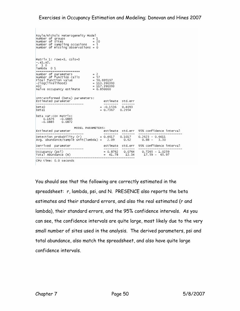
In the results browser, right click on the model itself and select “view model

output”. This will open a page in notepad with the results of the model.



You should see that the following are correctly estimated in the

spreadsheet: r, lambda, psi, and N. PRESENCE also reports the beta

estimates and their standard errors, and also the real estimated (r and

lambda), their standard errors, and the 95% confidence intervals. As you

can see, the confidence intervals are quite large, most likely due to the very

small number of sites used in the analysis. The derived parameters, psi and

total abundance, also match the spreadsheet, and also have quite large

confidence intervals.

Documents

Exercise 7. Royle-Nichols Abundance Induced … in Occupancy Estimation and Modeling; Donovan and Hines 2007 Chapter 7 Page 1 5/8/2007 EXERCISE 7: ROYLE-NICHOLS ABUNDANCE INDUCED