Embed Size (px)
Citation preview

1
ggpogn
as5tmelFtpFwiig
bAs
gflpqrfst
sto
i2E
J
Downloaded Fr
Hugh GoyderCranfield University,
Shrivenham, Swindon SN6 8LA, UKe-mail: [email protected]
On the Modelling of NoiseGeneration in Corrugated PipesThe offshore oil and gas industry uses corrugated pipes because of their flexibility. Gasflowing within these pipes interacts with the corrugations and generates noise. This noiseis of concern because it is of sufficient amplitude to cause pipework vibration with thethreat of fatigue and pipe breakages. This paper examines the conditions that give rise tothe large noise levels. These conditions, for the occurrence of noise, are investigatedusing an eigenvalue approach, which involves the effect of damping due to losses fromthe pipe boundaries and pipe friction. The investigation is conducted in terms of reflec-tion conditions and shows why only few of the very many possible natural frequencies areselected. The conditions for maximum noise response are also investigated by means of anonlinear model of vortex shedding. Here, an approach is developed in which the netpower generated by each wavelength is calculated. DOI: 10.1115/1.4001977
IntroductionGas flowing within a pipe, which has internal corrugations, may
enerate large noise levels. The noise is of concern to the oil andas industry because it may be of sufficient amplitude to causeipework vibration that may lead to fatigue after only a few hoursf operation. Pipework failure with the consequent loss of gas isenerally unacceptable and, thus, a good understanding of theoise generation mechanism is essential.
Corrugated pipelines are used because they are flexible. Theyre called risers when they connect between a platform on theea-surface and equipment on the seabed. Such pipes may be00 m or 1000 m in length and around 0.2 m in diameter. Whenhese pipes are used on the seabed they are known as jumpers and
ay be shorter or longer than risers. Short corrugated pipes, forxample 20 m in length, are known to produce noise as well asonger lengths. An illustration of a corrugated pipe is shown inig. 1, which is based on ISO 13628-11 1. The gas flow within
he pipe passes over the carcass, which is designed to keep theipe open should the pressure within fall to zero. The carcass,ig. 2, which forms the corrugations, includes pockets or cavities,hich contain stagnant gas. A shear layer forms between the mov-
ng fluid within the pipe and the stagnant gas in the cavity and its the oscillation of these shear layers that is responsible for theeneration of the noise.
The production of noise from a corrugated pipe seems to haveeen first identified by Petrie and Huntley 2 and then by Ziada3. More recent publications are by Belfroid et al. 4, by Debutntunes and Moreira 5, by and Tonon et al. 6. The effect on
tructural vibration has been described by Goyder et al. 7.Practical experience of noise production shows that there is
enerally no problem at low flowrates but that with increasingow a threshold is exceeded and for higher flowrates noise will beroduced. The noise is periodic with a dominant fundamental fre-uency. As the flow rate is steadily increased the noise frequencyemains locked-on to a single frequency but will jump to a newrequency, typically a higher frequency, when the flow rate isufficiently increased. Similar behavior of lock-on occurs whilehe flow is being decreased.
Oil and gas companies must make a decision on how to operatehould the noise be produced. Some decide to operate only belowhe threshold velocity for the onset of noise. Others decide toperate with the noise present and then ensure that their equip-
Contributed by the Pressure Vessel and Piping Division of ASME for publicationn the JOURNAL OF PRESSURE VESSEL TECHNOLOGY. Manuscript received October 30,009; final manuscript received June 2, 2010; published online July 21, 2010. Assoc.
ditor: Njuki W. Mureithi.ournal of Pressure Vessel Technology Copyright © 20
om: http://pressurevesseltech.asmedigitalcollection.asme.org/ on 03/10/20
ment will withstand the noise and vibration. It is worth noting thatsubsea jumpers may make a noise but that this may not be appar-ent to the operators, thus, possibly allowing a potential damagesource to go unnoticed.
This paper addresses the problem of how a corrugated pipe canbe assessed for conditions that lead to unacceptable noise. Thereare two main difficulties. i A corrugated pipe is usually termi-nated by a very complicated system of pipework at each end. Thisconfiguration makes computer modeling very difficult because ofthe differing length scales involved; a very long length of corru-gated pipe with many short lengths of pipe in the terminations.This problem is tackled first. ii Only limited data is availableconcerning the source strength and behavior. A typical problem isthe need to interpolated and extrapolate from a few measurementsof corrugation noise. A basis for such extrapolation is given. Boththese problems are tackled in a novel manner in this paper.
2 The Noise SourceIt is well known that flow over a cavity containing stagnant
fluid causes oscillations in the shear layer, which forms betweenthe moving and stagnant fluid 8. In this application, the movingflow is within the pipe and the stagnant flow is within the cavitiesof the carcass. The oscillations of the shear layer, sometimescalled vortex shedding set up an axial acoustic wave within thepipe. The acoustic wave causes all the shear layers on all thecavities to become synchronized to the acoustic wave. The shearlayers and acoustic wave form feedback loops in which the shearlayer is a source for the acoustic wave and the acoustic waveassists the formation of the shear layer. Only axial waves areconsidered here. The possibility of high frequency waves withwavelengths of the order of a pipe diameter could be an additionalproblem but the associated frequencies are beyond those whichhave been observed within the work considered here.
The basic equation that relates the frequency of shear layeroscillation to the flow velocity is due to Rossiter and is describedin detail by Howe 8. The equation is
St =fW
U01
where St is the Strouhal number, f is the frequency of oscillation,W is the width of the cavity, and U0 the flow velocity in the pipe.This equation has been checked experimentally by Belfroid 4.He treated the width as a free parameter and determined whichdimension best fits the data. Additionally, he determined best val-ues for the Strouhal number although he noted that the cavitywidth is not a simple quantity and that some account may have to
be taken of the rounding of the cavity edges.AUGUST 2010, Vol. 132 / 041304-110 by ASME
14 Terms of Use: http://asme.org/terms

uasTo
3
p
Ft sur
Fl
Fp arr
Fa
0
Downloaded Fr
The oscillations of the shear layer are considered to be a vol-me velocity source of the monopole or dipole type. The sourcesre illustrated diagrammatically in Fig. 3. Both these types ofource will generate acoustic wave in the pipe. The recent work ofonon et al. 6 suggested that the dipole source is more likely toccur.
The Acoustic Boundary ConditionsAcoustic plane waves propagate in both directions within the
ipe. A resonant condition is set up when the waves are reflected
3
34
5
6
7
8
ig. 1 Construction of corrugated pipe: „1… antifriction layer, „2ensile armor, „5… back-up pressure armor, „6… interlocked pres
Flow
Shear Layer
Cavity
ig. 2 Corrugated pipe carcass showing cavity and shearayer
Flow
ig. 3 Diagrammatic representation of pipe, flow, cavities, andoles „shown as straight arrows… or dipoles „shown as curved
L1 Side branch
Corru
S
S1
ig. 4 A corrugated pipe of length L and cross-sectional area S
rea S1 and a T-junction where the pipe cross-sectional area chan41304-2 / Vol. 132, AUGUST 2010
om: http://pressurevesseltech.asmedigitalcollection.asme.org/ on 03/10/20
from boundaries at each end. The consideration of boundary con-ditions forms in important part of this investigation because it isfound that the boundary conditions are responsible for determin-ing which acoustic natural frequencies will be selected by thevortex shedding mechanism.
Typically, a pipe carrying flow cannot have closed or open endsand consequently it is not immediately obvious how standingwaves are formed. As an illustrative, and not untypical, examplethe configuration shown in Fig. 4 will be investigated. Here a sidebranch at the left-hand end forms one boundary while the changein cross-section at the right-hand end provides a second boundary.These are simple boundary conditions. In a real configuration,they can be much more complicated with tens or hundreds of sidebranches and changes in cross-section. A method for handlingsuch boundary conditions is required.
The boundary conditions for this configuration or any morecomplicated configuration are best described by means of reflec-tion coefficients. A reflection coefficient is the ratio of the pressurein the reflected wave to the pressure in the incoming wave. At theright-hand end, in this example, the change in cross-section has areflection coefficient 2 given by
1
2
3
4
3
5
6
7
8
uter layer of tensile armor, „3… antiwear layer, „4… inner layer ofe armor, „7… internal pressure sheath, and „8… carcass
ear layers. The sources from the cavities can be either mono-ows….
Change in cross section
d pipeS2
erates between a side branch of length L1 and cross-sectional
1
2
… o
sh
L
gate
op
ges to S2.Transactions of the ASME
14 Terms of Use: http://asme.org/terms

wrt
wfqstflqpcs
fcae
patebtnl
4
prbo
Fttfi
J
Downloaded Fr
2 =1 − r
1 + r2
here r is the ratio of new area to the existing area, in this case=2S2 /S. The two arises from the waves being able to exit theee in two directions.
For the left-hand condition the reflection coefficient is given by
1 = −r
r − 2i cot kL13
here in this case r=S1 /S and the wave number k= /c. Therequency is in radians per second =2f where f is the fre-uency in hertz and c is the speed of sound. The length of theide branch is L1. Both reflection coefficients have a magnitudehat lies between 0 and 1. They may also have a phase. The re-ection coefficient for the right-hand end is constant with fre-uency while for the left it is dependant on frequency. This de-endence is illustrated in Fig. 5. It can be seen that the reflectionoefficient is small except at frequencies that correspond to atanding wave in the side branch. These occur when
kL1 =L1
c= 2n − 1
2, n = 1,2,3, . . . 4
Thus, the left-hand boundary is a good reflector only at somerequencies and will allow waves to escape at most other frequen-ies. In allowing waves to escape from the pipe, the boundariesct in a way that is similar to a damping device—they allownergy to leave the corrugated pipe.
Reflection coefficients can be calculated using proprietary com-uter codes, which can take into account complicated pipeworkrrangements. Note that the whole pipework system does not haveo be modeled. It is sufficient to form two models each of whichmbrace only that pipework, which is in the vicinity of eachoundary of the corrugated pipe. This avoids the need to introducehe corrugated pipe in the acoustic simulation, thus, avoiding theeed to have a long length scale, the corrugated pipe, and a shortength scale for the side branches in the terminations.
Eigenvalue AnalysisWhat are the natural frequencies of the acoustic wave in the
ipe configuration of Fig. 4? Or more generally what are the natu-al frequencies of a pipe bounded by two discontinuities modeledy reflection coefficients? A typical formula for a pipe with closed
0 2 4 6 8 100.001
0.005
0.010
0.050
0.100
0.500
1.000
Ω L1c
Ref
lect
ion
Coe
ffic
ient
ig. 5 Modulus of reflection coefficient for a side branch plot-ed on logarithmic scale. Here, the area ratio S1 /S=0.1 and L1 ishe length of the side branch. The peaks in the reflection coef-cient coincide with resonances in the side branch.
r open ends gives the natural frequencies as
ournal of Pressure Vessel Technology
om: http://pressurevesseltech.asmedigitalcollection.asme.org/ on 03/10/20
fn =nc
2L, n = 1,2,3. . . 5
where fn is the nth natural frequency in hertz. For a long pipe,such as those being considered here, the natural frequencies cal-culated using Eq. 5 are closely spaced. Thus, with a speed ofsound of 400 m/s typical for methane and L=500 m, the spac-ing of natural frequencies is 0.4 Hz. Thus, there are apparentlyvery many natural frequencies for the vortex shedding mechanismto select. However, only very few are observed in practice.
A more detailed analysis that includes the effects of energy lossfrom boundaries may be performed by means of an eigenvaluecalculation. The starting point is to note that the waves in the pipemay be modeled by
p = Ae−ikx + Beikx 6
where p is the pressure at location x along the pipe and A and Bare the amplitudes of the waves propagating in the positive andnegative directions, respectively. This analysis assumes that thewave motion is harmonic with frequency dependence exp+it.As before k is the wave number and is equal to /c. The samewave number is applicable for both the positive and negativewaves for the case where the flow velocity is small compared withthe speed of sound small Mach number. This is usually the casefor the configuration of a riser or jumper but the equation wouldhave to be modified if large Mach numbers are encountered.
Two equations may now be developed using the reflection co-efficients. At the left-hand end x=0 the wave of amplitude B isincoming and the wave of amplitude A is reflected. Hence, thereflection coefficient is related to the wave amplitudes by
1 =A
B7
In contrast at the right-hand end x=L the wave with amplitudeA is incoming with the reflected wave having amplitude B. Also,at this end, the waves are influenced by their exponential term,thus,
2 =BeikL
Ae−ikL 8
These equations may be organized into a matrix form as fol-lows:
1 − 1
− 2 e2ikL A
B = 0
0 9
In a more general analysis the terms on the right-hand sidewould contain acoustic source terms. As in a standard eigenvalueproblem the determinate of the matrix must be zero for values ofA and B to exist with no source terms. Thus,
e2ikL − 12 = 0 10By moving the second term to the right-hand side, taking the
log of both sides and remembering that the log function is multi-valued the last equation may be written as
kL =L
c= −
i
2ln 12 + n, n = 1,2,3. . . 11
For the special case of 1 and 2 real and equal to 1 fullreflections Eq. 5 is recovered. However, for the case wherethere is only partial reflection then complex values must be usedfor . In particular, this gives rise to complex frequencies, whichare the poles of the eigenvalue problem. Hence,
nr =
c1arg12 + n 12
L 2
AUGUST 2010, Vol. 132 / 041304-3
14 Terms of Use: http://asme.org/terms

wsatwcmdc
ttcitaqclc
obSttnTict
v
poldvtntti
Fwti
0
Downloaded Fr
ni =
− c
2Lln12 13
here the complex frequency is written as n=nr + in
i super-cript r for real and i for imaginary. Note that 1 and 2, as wells having magnitude of, at most 1, have negative real values and,hus, have restricted phase angles. In Eq. 12, the value of n ill, therefore, outweigh the argument of the reflection coeffi-
ients for all but the first few n and, thus, Eq. 5 is still approxi-ately true. The damping is described by Eq. 13 and is depen-
ant on the log of the magnitude of the product of the reflectionoefficients.
It is interesting to consider what happens as one of the reflec-ion coefficients drops to zero. If both coefficients start as 1.0 thenhe poles lie on the real axis. As the product of reflection coeffi-ients get smaller the poles move into the complex plane accord-ng to Eq. 13. As the product drops to zero, Eq. 13 shows thathe poles have moved to infinity. This limiting case corresponds ton anechoic condition for which there are no acoustic natural fre-uencies. Thus, Eqs. 12 and 13 remain valid for all boundaryonditions. In particular, note that due to damping the poles willie off the real axis with those poles with least damping beinglosest to the axis.
For the particular case of the configuration of Fig. 4 the locationf the poles eigenvalues is given in Fig. 6. Here, for the sideranch model, L /L1 is 100 and S /S1=10 while for the tee/S2=1. An exact calculation has been made using Eq. 10. Note
hat the curve is made up of points where each point correspondso an eigenvalue. This calculation confirms that there are a largeumber of closely spaced natural frequencies as suggested by Eq.5. The relationship between Fig. 6 and Fig. 5 should be noted.he poles lie along a curve that is the same as that in Fig. 5 but is
nverted. Examination of Eq. 13 confirms that this observation isompletely correct and provides a simple method for determininghe poles of the configuration.
The acoustic damping ratio can be calculated from the polealues by dividing the imaginary part of the pole by the real part.
As illustrated in this example and as found in practice, very fewoles have small imaginary part and, thus, small damping. It isnly at those natural frequencies where the reflection coefficient isarge and little energy is lost through the boundaries that theamping is small. It is these poles that are most susceptible to theortex shedding mechanism. The shear layers provide energy tohe system in the sense of negative damping. Thus, the addition ofegative damping will cause the poles to cross the axis and go tohe unstable half of the complex plane. In this Fourier formula-ion the unstable half of the complex plane is the lower half. This
0 200 400 600 800 10000
1
2
3
4
Real part of natural frequency ΩrLc
Imag
inar
ypa
rtof
natu
ralf
requ
encyΩ
i Lc
ig. 6 Complex natural frequencies „poles… of system in Fig. 4ith L /L1=100, S1 /S=0.1, and S2 /S=2. The horizontal axis is
he real part of the natural frequency and the vertical axis is themaginary part.
s in contrast to the Laplace formulation where the unstable half is
41304-4 / Vol. 132, AUGUST 2010
om: http://pressurevesseltech.asmedigitalcollection.asme.org/ on 03/10/20
the right half plane. In summary, the fact that only a few poleshave small damping explains why only a few resonant frequenciesand not all those suggested by Eq. 5 are observed in practice.
5 Attenuation With DistanceAs well as energy lost at the boundaries a further source of
energy dissipation is attenuation along the pipeline. Belfroid et al.4 consider various types of attenuation and use a standard modelin which Eq. 6 is modified with the introduction of an attenua-tion parameter. The modified equation for the pressure now reads
p = Ae−xe−ikx + Bexeikx 14
where is a small parameter of order 0.01 m−1. The simplestmethod for dealing with this additional source of damping is tomake k and, hence, complex. This enables the previous eigen-value calculation to proceed as before but now there is an addi-tional complex term. With this term Eq. 13 is modified to
ni = c −
c
2Lln12 15
This merely moves the imaginary part of each eigenvalue fur-ther upward from the horizontal axis. Thus, the shear layermechanism must provide negative damping that overcomes at-tenuation with distance as well as losses from the boundaries tomove the poles to the unstable half of the complex plane.
For the acoustic system to produce noise it is necessary for it tobecome unstable and for the poles to move to the unstable half ofthe complex plane. The vortex shedding mechanism providesnegative damping and those poles closest to the real axis can bemoved across the axis allowing instability. Poles deep within thestable part of the complex plane with corresponding large damp-ing will not become unstable because the negative dampingmechanism provided by vortex shedding cannot overcome thelarge damping values. The eigenvalue analysis enables these vul-nerable poles to be identified. The next step is to determine thestrength of the source and how it provides negative damping.
6 Source AnalysisThe mechanism of vortex shedding across a cavity has been
investigated in many circumstances. The phenomenon is nonlinearand involves the rolling up of the shear layer to produce vortices.For small amplitudes the shear layer oscillations add energy to thesystem and, thus, act as a source of negative unstable damping.However, for large amplitudes the shear layer absorbs energy and,thus, acts as positive damping. The noise in the pipe evolves inresponse to these nonlinear energy sources and sinks.
There are at least two ways in which the shear layer can interactwith the acoustic wave. These alternative interactions are illus-trated in Fig. 7. If the lump of fluid adjacent to the shear layer andin the mouth of the cavity oscillates in a pistonlike manner, theneach cavity provides a monopole source. Such sources have beenfrequently observed in deep cavities where resonance within thecavity causes large amplitudes of motion in the mouth. Alterna-
p2
p1qU0
a
q
U0
q
b
Fig. 7 A cavity with a shear layer. „a… The shear layer producesa monopole source with fluid pumped pistonlike into and out ofthe cavity. „b… A dipole source with the shear layer flapping in ahingelike manner.
tively, the shear layer and the adjacent fluid can rotate, possibly
Transactions of the ASME
14 Terms of Use: http://asme.org/terms

flcafwma
pwtesi
siccidibcwdl
gsbrMatsdpo
psod
Favp
J
Downloaded Fr
apping in a hingelike manner from the separation edge of theavity. In this case, each cavity acts like a dipole source. Possiblymixture of these two motions can occur. It should be noted that
or the long wavelengths being considered there is no resonanceithin the cavity and the oscillations of the fluid in the mouthust simply compress the gas in the cavity, which will behave inspringlike manner with no inertia.Recent experiments by Tonon et al. 6 suggested that the di-
ole mechanism is more likely in which a grazing flow interactingith the shear layer and coordinated by an acoustic plain wave in
he pipe produces a dipole source. Tonon et al. are able to make anstimate of the noise produced in their system based on computerimulations of a shear layer. This work is very useful in identify-ng the fundamental cause of the noise in corrugated pipes.
The approach adopted here starts from the engineering circum-tances where some noise data is available and it is necessary tonterpolate and extrapolate to other similar circumstances. For thisase a simple noise model is required that will facilitate this pro-ess. The noise model uses an energy approach and is based ondeas that have been developed for the monopole case. Although aipole source is being considered, it is assumed that the behaviors analogous to the monopole case and this seems reasonable sinceoth are consequences of the oscillation of a shear layer over aavity. In particular, the key issue to model is the source strength,hich must increase when the acoustic velocity is small and thenecreases and become a sink as the acoustic velocity becomesarge.
A very complete set of data for the monopole source has beenenerated in experiments by Graf and Ziada 9. This data ishown in Fig. 8. The data model the source strength in terms ofoth the Strouhal number and the acoustic velocity. This data haveeceived some recent confirmation with numerical simulations by
artinez-Lera and Schram 10. The data in Fig. 8 are expresseds a complex impedance with the real part which is in-phase withhe velocity describing the energy supplied or removed by theource and the imaginary part out-of-phase with the velocityescribing the extra stiffness loading of the source. It is antici-ated that the data for the dipole source will be similar. However,nly limited proprietary data from actual occurrences is available.
The modeling starts by assuming that resonant conditions areresent in the pipe with an acoustic wave that is sinusoidal in bothpace and time. An appropriate frequency to consider would bene that the eigenvalue analysis has identified as having small
1.0 0.5 0.0 0.5 1.0
1.0
0.5
0.0
0.5
1.0
0.010.018
0.032
0.056
0.1
0.3
0.4
0.5
0.6
0.7
0.8
0.91.0
RealImag
inar
y
a
ig. 8 The nondimensional acoustic impedance of a shear layxis while the imaginary part is shown vertically. The “spiral” linelocity. The “radial” lines correspond to constant Strouhal nuart „b… includes larger acoustic amplitudes.
amping. In this circumstance, the net energy supplied by all the
ournal of Pressure Vessel Technology
om: http://pressurevesseltech.asmedigitalcollection.asme.org/ on 03/10/20
sources in each corrugation must balance the energy dissipated bythe damping. Furthermore, when the acoustic amplitude is smallthe shear layers must act as a source providing negative dampingand when the amplitude is large the shear layers must act as a sinkabsorbing energy.
The data of Graf and Ziada provide exact modeling of thispositive or negative feedback for the monopole source. Figure 9shows an example of this behavior for the case of a Strouhalnumber of 0.4. This is an appropriate Strouhal number for corru-gated pipes. The data are extracted from Fig. 8 and a quadraticcurve fitted. The source, thus, has the form
s = AuU0
uU0
− B 16
where s is the source strength, u is the acoustic velocity, and U0the velocity of the mean flow. The parameters A and B are con-stants, which may easily be determined for the monopole casefrom the Graf and Ziada data. For the case being considered herethe two parameters A and B must be determined from measureddata. The key assumption is that the quadratic form is similar forboth the monopole and dipole cases. The source model here is
1.0 0.5 0.0 0.5
1.0
0.5
0.0
0.5
1.0
0.010.018
0.032
0.056
0.1
0.180.32 0.5
0.3
0.4
0.5
RealImag
inar
y
b
from Graf and Ziada. The real part is shown on the horizontalcorrespond to constant acoustic amplitude normalized by flowers. Part „a… includes smaller acoustic amplitudes only while
0.0 0.1 0.2 0.3 0.4 0.5 0.6
0.05
0.00
0.05
Normalised acoustic velocity uU0
Aco
ustic
impe
danc
eu
U0f
St,uU
0
Fig. 9 Real part of acoustic impedance of a shear layer for aStrouhal number of 0.4 as a function of acoustic velocity udivided by mean flow velocity U0. The function f„St,u /U0… isobtained, together with the points from Fig. 8. The smooth
eresmb
curve is a fit of Eq. „16… to this data.
AUGUST 2010, Vol. 132 / 041304-5
14 Terms of Use: http://asme.org/terms
oiTda
atswcpfa
is
w
g
wdgpv
wetom
e0ddvrwt
nocdad
7
mpaerrsvapa
0
Downloaded Fr
nly for the real part of the source impedance the imaginary parts available for the monopole source but not for the dipole case.he imaginary part expresses the change in the speed of soundue to the presence of the corrugations. Fortunately, for an energynalysis only the real part is needed.
The effect of all the cavities must be combined to give themplitude of the acoustic wave. The approach is to assume thathe response to the shear layer in each cavity is local with eachhear layer responding to the local acoustic velocity. Along oneavelength of the standing wave there are a range of conditions
hanging from pressure antinodes with zero acoustic velocity toressure nodes with maximum acoustic velocity. The model isormed by working out the net effect of all the carcass cavitieslong a single representative wavelength.
The acoustic velocity depends on the location along the stand-ng wave. If there are N cavities along one wavelength of thetanding wave then the velocity at location n is given by
u = U sin2n
N 17
here U is the maximum acoustic velocity along the wavelength.The acoustic power generated by the dipole in each cavity is
iven by
wn =1
2s u
U02
=1
2s U
U02
sin22n
N 18
here the source s is modeled above in Eq. 16. Note that s alsoepends on u and, thus, on Eq. 17. It can be seen that the powerenerated by each dipole is a very complicated expression de-ending on the location within each wavelength and the localalue of acoustic velocity.
The energy analysis proposed here considers one completeavelength of a standing wave. For each flow velocity it is nec-
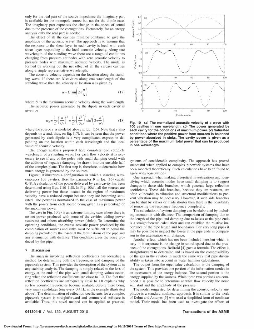
ssary to see if any of the poles with small damping could withhe addition of negative damping, be drawn into the unstable halff the complex plane. The first step is, therefore, to determine howuch energy is generated by the sources.Figure 10 illustrates a configuration in which a standing wave
mbraces 100 cavities. Here the parameter B in Eq. 16 equals.48. A calculation of the power delivered by each cavity has beenetermined using Eqs. 16–18. In Fig. 10b, all the sources areelivering power but those located in the region of maximumelocity have a reduced output because they are becoming satu-ated. The power is normalized to the case of maximum powerith the power from each source being given as a percentage of
he maximum power.The case in Fig. 10c is an extreme limiting case where there is
o net power produced with some of the cavities adding powersources and others absorbing power sinks. To determine theperating conditions, the excess acoustic power produced by theombination of sources and sinks must be sufficient to equal theamping provided by the losses at the terminations of the pipe andny attenuation with distance. This condition gives the noise pro-uced by the pipe.
DiscussionThe analysis involving reflection coefficients has identified aethod for determining both the frequencies and damping of the
ipework system. This provides the description of the system as inny stability analysis. The damping is simply related to the loss ofnergy at the ends of the pipe with small damping values occur-ing when the reflection coefficients are close to 1.0. The fact thateflection coefficients are infrequently close to 1.0 explains whyo few acoustic frequencies become unstable despite there beingery many candidates one every 0.4 Hz in the example illustratedbove. The determination of reflection coefficients for a complexipework system is straightforward and commercial software is
vailable. Thus, this novel method can be applied to practical41304-6 / Vol. 132, AUGUST 2010
om: http://pressurevesseltech.asmedigitalcollection.asme.org/ on 03/10/20
systems of considerable complexity. The approach has provedsuccessful when applied to complex pipework systems that havebeen modeled theoretically. Such calculations have been found toagree with observations.
One approach when making theoretical investigations and iden-tifying which acoustic modes have small damping is to suggestchanges in those side branches, which generate large reflectioncoefficients. These side branches, because they are resonant, areoften vulnerable to vibration and structural modifications to pre-vent vibration may be necessary. However, if such side branchescan be shut by valves or made shorter then there is the possibilityof removing the resonance frequency completely.
The calculation of system damping can be elaborated by includ-ing attenuation with distance. The comparison of damping due tothe length of the pipe and damping due to losses at the pipe endsis a straightforward calculation and can establish the relative im-portance of the pipe length and boundaries. For very long pipes itmay be possible to neglect the losses at the pipe ends in compari-son to the attenuation with distance.
Another effect, which has not been included here but which iseasy to incorporate is the change in sound speed due to the pres-ence of the corrugations. Belfroid 4 gave a formula. The effect isstraightforward to determine and is based on the compressibilityof the gas in the cavities in much the same way that pipe disten-sibility is taken into account in water hammer calculations.
The output from the eigenvalue calculation is the damping ofthe system. This provides one portion of the information needed inan assessment of the energy balance. The second portion is theenergy supplied by the sources. When these two portions are com-bined it is possible to determine at what flow velocity the noisewill start and the amplitude of the pressure.
The model suggested for determining the acoustic velocity am-plitude is a standard nonlinear approach. It is similar to the workof Debut and Antunes 5 who used a simplified form of nonlinear
0 20 40 60 80 100
1.0
0.5
0.0
0.5
1.0
Aco
ustic
Vel
ocity
a
0 20 40 60 80 100
0.0
0.5
1.0
1.5
Cav
ityPo
wer
b
0 20 40 60 80 1004
3
2
1
0
1
2
Cavity number
Cav
ityPo
wer
c
Fig. 10 „a… The normalized acoustic velocity of a wave with100 cavities in one wavelength. „b… The power generated byeach cavity for the conditions of maximum power. „c… Saturatedconditions where the positive power from sources is balancedby power absorbed in sinks. The cavity power is given as apercentage of the maximum total power that can be producedin one wavelength.
model. Their model has been used to investigate the effects of
Transactions of the ASME
14 Terms of Use: http://asme.org/terms

npm
ZtctewUdldo
8
A
t
N
J
Downloaded Fr
onperiodic separation of corrugations. The novel approach in thisaper is to develop a method for conditions where there are veryany sources.It should be stressed that the shear layer data from Graf and
iada was collected on a different system a monopole source tohat considered here and that consequently it is not directly appli-able to the dipole source created by the corrugations. However,he general form of the data are likely to be similar. Examples ofquivalent earlier data are that of Coltman 11 and Elder 12,here both show a spiral form for the shear layer impedance.ntil equivalent data can be collected for a corrugated pipe thisata provides a good basis for understanding and modeling shearayers. However, what is needed is a good set of data for theipole case that mirrors the very full set of data, which has beenbtained by Graf and Ziada for the monopole case.
ConclusionsThe following conclusions may be drawn.
1. The acoustic losses at the boundaries of a corrugated pipeprovide an effect equivalent to damping. The boundary con-ditions, including this damping effect may be usefully mod-eled using reflection coefficients. An eigenvalue analysisthen shows how poles with small damping are related toreflection coefficients that are close to 1.0.
2. Although a long pipe has very many natural acoustic fre-quencies, only a very few are excited in practice. The se-lected frequencies are those for which the reflection coeffi-cients are large and the damping is small.
3. A full mathematical development for the acoustic poles of ariser has been formulated enabling these to be calculatedfrom a simple equation once the reflection coefficients areknown. See Eqs. 12, 13, and 15.
4. When use is made of a detailed shear layer model it is seenthat within one wavelength there will be locations that addenergy to the system and other locations that remove energy.A general model for one wavelength is constructed thatgives the net energy production or absorption.
5. An energy approach is suggested as a method for determin-ing noise from corrugated pipes. The terms in the energyequation include losses at the boundaries, absorption due tofriction and production and dissipation at cavities. This ap-proach is applicable when some data is available and there isa need to interpolate or extrapolate. It is clear that muchmore data is needed to enhance and validate the proposedenergy method.
cknowledgmentThe author acknowledges the support of Cranfield University at
he Defence Academy of the United Kingdom.
omenclatureA, B amplitudes of pressure waves in pipe PaA, B constants in source equation.
L length of corrugated pipe mL1 length of side branch mN number of corrugations in one wavelength
ournal of Pressure Vessel Technology
om: http://pressurevesseltech.asmedigitalcollection.asme.org/ on 03/10/20
S cross-sectional area of pipe m2S1 cross-sectional area of side branch m2S2 cross-sectional area of each pipe in tee junc-
tion m2St Strouhal number
U0 gas flow velocity m s−1U maximum acoustic velocity in pipe m s−1c speed of sound m s−1f frequency Hz
fn natural frequency the nth Hzi imaginary unit −1k wave number= /cn integer, 1, 2, 3…p acoustic pressure Par area ratio for reflection coefficients acoustic source for one cavityu acoustic velocity in pipe
wn acoustic power from one cavity Nm/sx distance along pipe mz acoustic impedance kg m−4 s−1 attenuation coefficient m−1 reflection coefficient gas density kg m−3 frequency radians per second=2f
n natural frequency in radians per second
References1 ISO 13628-11, “Petroleum And Natural Gas Industries—Design and Operation
of Subsea Production Systems—Part 11: Flexible Pipe Systems for Subsea andMarine Applications,” 2007-09 15.
2 Petrie, A. M., and Huntley, I. D., 1980, “The Acoustic Output Produced by aSteady Airflow Through a Corrugated Duct,” J. Sound Vib., 701, pp. 1–9.
3 Ziada, S., and Buhlmann, E. T., 1991, “Flow Induced Vibration in Long Cor-rugated Pipes,” International Conference on Flow-Induced Vibrations, IM-echE, Brighton, UK.
4 Belfroid, S. P. C., Swindell, R., and Tummers, R., 2008. “Flow Induced Pul-sations Generated in Corrugated Tubes,” Ninth International Conference onFlow-Induced Vibration, Prague, Czech Republic, Jun. 3–Jul. 3.
5 Debut, V., Antunes J., and Moreira M., 2008, “Flow-Acoustic Interaction inCorrugated Pipes: Time Domain Simulation of Experimental Phenomena,”Ninth International Conference on Flow-Induced Vibration, Prague, Czech Re-public, Jun. 3–Jul. 3.
6 Tonon, D., Landry, B. J. T., Belfroid, S. P. C., Willems, J. F. H., Hofmans, G.C. J., and Hirschberg, A., 2010, “Whistling of a Pipe System With MultipleSide Branches: Comparison With Corrugated Pipes,” J. Sound Vib., 329, pp.1007–1024.
7 Goyder, H. G. D., Armstrong, K., Billingham, L., Every, M. J., Jee, T. P., andSwindel, R. J., 2006, “A Full Scale Test for Acoustic Fatigue in Pipework,”ASME PVP, ICPVT, pp. 11–9377.
8 Howe, M. S., 2004, Acoustics of Fluid-Structure Interactions, Cambridge Uni-versity Press, Cambridge.
9 Graf, H. R., and Ziada, S., 1992, Flow Induced Acoustic Resonance in ClosedSide Branches: An Experimental Determination of the Excitation Source,”ASME Symposium on Flow-Induced Vibration and Noise, ASME PVP, NewYork, Vol. 247.
10 Martínez-Lera, P., Schram, C., Föller, S., Kaess, R., and Polifke, W., 2009,“Identification of the Aeroacoustic Response of a Low Mach Number FlowThrough a T-Joint,” J. Acoust. Soc. Am., 1262 582–586.
11 Coltman J. W., 1968, “Sound Mechanism of the Flute and Organ Pipe,” J.Acoust. Soc. Am., 444 983–992.
12 Elder S. A., 1978, “Self-Excited Depth-Mode Resonance for a Wall-MountedCavity in Turbulent Flow,” J. Acoust. Soc. Am., 643 877–890.
AUGUST 2010, Vol. 132 / 041304-7
14 Terms of Use: http://asme.org/terms