Embed Size (px)
Citation preview
FREE VIBRATION OF RODS, BEAMS AND FRAMES
USING SPECTRAL ELEMENT METHOD
A THESIS
Submitted by
Anusmita Malik
For the award of the degree
of
MASTER OF TECHNOLOGY
STRUCTURAL ENGINEERING DIVISION DEPARTMENT OF CIVIL ENGINEERING
NATIONAL INSTITUTE OF TECHNOLOGY, ROURKELA 769008 May 2013
CERTIFICATE
This is to certify that the thesis entitled “FREE VIBRATION OF RODS, BEAMS AND
FRAMES USING SPECTRAL ELEMENT METHOD” submitted by Anusmita Malik in
partial fulfilment of the requirement for the award of Master of Technology degree in Civil
Engineering with specialization in Structural Engineering to the National Institute of
Technology, Rourkela is an authentic record of research work carried out by her under my
supervision. The contents of this thesis, in full or in part, have not been submitted to any
other Institute or University for the award of any degree or diploma.
Project Guide
Rourkela-769008 Dr. Manoranjan Barik
Date: Associate Professor
Department of Civil Engineering
i
ACKNOWLEDGEMENT
First and foremost, praise and thanks goes to my God for the blessing that has been bestowed
upon me in all my endeavours.
I am deeply indebted to Dr. Manoranjan Barik, Associate Professor, my advisor and guide,
for the motivation, guidance, tutelage and patience throughout the research work. I appreciate
his broad range of expertise and attention to detail, as well as the constant encouragement he
has given me over the years. There is no need to mention that a big part of this thesis is the
result of joint work with him, without which the completion of the work would have been
impossible.
I extend my sincere thanks to the Head of the Civil Engineering Department Prof. N. Roy,
for his advice and unyielding support over the year.
I would like to take this opportunity to thank my Parents and my sister for their unconditional
love, moral support, and encouragement for the timely completion of this project.
I am grateful for friendly atmosphere of the Structural Engineering Division and all kind and
helpful professors that I have met during my course.
I express my most sincere admiration to my friends, (in no particular order)
MonalishaPriyadarsini, Krishna Kumar, VenkyKotipalli and to all my classmates for
their cheering up ability which made this project work smooth.
ii
So many people have contributed to my thesis, my education, and it is with great pleasure to
take the opportunity to thank them. I apologize, if I have forgotten anyone.
Anusmita Malik
Roll No:211CE2027
M.Tech. (Structural Engineering)
National Institute of Technology
Rourkela-769008,Odisha, India
iii
PREFACE
In the field of engineering the dynamic characteristics of a structure are of utmost importance
for which these need considerable attention for greater accuracy. In today’s world of digital
computation the researchers’ thrust is always towards this accuracy which may be achieved
with a computational cost. The finite element method (FEM) has taken its place as a
competent numerical tool to analyse the dynamics of a structure. Though it can handle the
problems efficiently, it is limited to low frequency wave modes. When the structure vibrates
with high frequency, the finite element method needs to be modelled with very large number
of elements to capture all necessary frequencies of higher modes. The availability of
computational softwares to have analytical solutions with Symbolic Algebra has enabled the
researchers to handle the tedious algebraic expressions with less effort. These softwares are
MATHEMATICA, MAPLE, Math CAD etc to name a few and MAT LAB to some extent.
The exact solution of the governing differential equations
for the vibration problems with higher modes of vibration can be formed by using the shape
functions which are frequency dependent. Thus using these frequency dependent shape
functions the stiffness matrix which is dependent on the frequency can be formulated which
is known as the Dynamic Stiffness Matrix (DSM). Once this Dynamic Stiffness Matrix for an
element is formulated the global Dynamic Stiffness Matrix is obtained by following the
procedure similar to that of the Finite Element Method (FEM). The great advantage of such a
matrix is that even higher frequencies of a structure can be obtained by considering only few
elements thus minimizing the computational cost.
In this thesis the higher modes of free vibration
frequencies have been obtained for rods, beams and frames. In case of rods and beams up to
the twentieth mode have been computed by considering only 2 spectral elements. In case of
iv
frame each member is considered as a single element and the frequencies even for higher
modes have been achieved accurately. In some examples the number of finite elements
required to converge to the exact analytical solution has been shown and it was noted that
even for number of finite elements up to 200, the results couldn’t converge even for the lower
modes.
v
CONTENTS
Title page No
Acknowledgement............................................................................................................i
Preface..............................................................................................................................iii
Contents............................................................................................................................v
List of figures...................................................................................................................vii
List of tables....................................................................................................................viii
List of symbols.................................................................................................................ix
1 Introduction.........................................................................................................1
1.1 Theoretical Background..................................................................................1
1.1.1 Dynamic Stiffness Method............................................................................2
1.1.2 Spectral Analysis Method..............................................................................3
1.1.3 Spectral Element Method................................................................................3
1.1.4 Present Scope of Investigation........................................................................4
2 Literature Review................................................................................................6
3 Theoretical Formulation......................................................................................14
3.1 Spectral Element Formulation of rod.............................................................15
3.2 Spectral Element Formulation of Euler-Bernoulli beam................................19
3.3 Spectral Element Formulation of Timoshenko beam.....................................25
3.4 Spectral Element Formulation of Frame........................................................32
4 Results and Discussions.....................................................................................39
5 Conclusion..........................................................................................................56

vi
Scope of future work.........................................................................................58
References.........................................................................................................59
vii
LIST OF FIGURES
S. no Titles Page No
1 Sign convention for the rod element...............................................................17
2 Sign convention for the Euler-Bernoulli beam element..................................21
3 Sign convention for the Timoshenko-beam element......................................29
4 forces and displacements at the nodes of a member.......................................34
5 Natural frequencies of first mode...................................................................52
6 Natural frequencies of twenty modes.............................................................52
7 frame 1............................................................................................................53
8 frame 2............................................................................................................53
8 frame 3............................................................................................................53
viii
LIST OF TABLES
Table no. Title Page No
1 Comparison of natural frequencies of fixed-free rod..................................40
2 Comparison of natural frequencies of fixed-fixed rod................................41
3 Comparison of natural frequencies of Euler-Bernoulli fixed-free beam.....42
4 Natural frequencies of Euler-Bernoulli simple-simple beam.......................43
5 Natural frequencies of Euler-Bernoulli Fixed-simple beam.........................44
6 Natural frequencies of Euler-Bernoulli Fixed-fixed beam...........................45
7 Comparison of natural frequencies of Timoshenko fixed-fixed beam.........46
8 Comparison of natural frequencies of Timoshenko pinned-pinned beam....48
9 Natural frequencies of Timoshenko fixed-free beam...................................50
10 Natural frequencies of Timoshenko fixed-pinned beam..............................51
11 Natural frequencies of frame1 & 2...............................................................54
12 Natural frequencies of frame3......................................................................55
ix
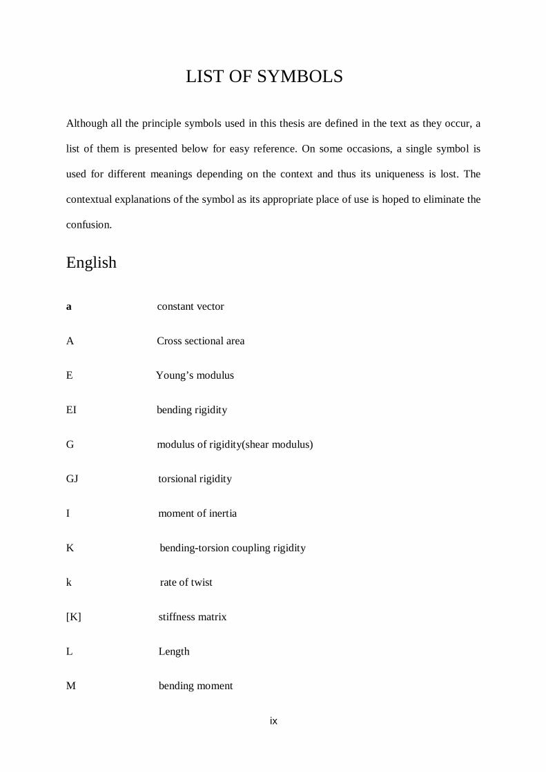
LIST OF SYMBOLS
Although all the principle symbols used in this thesis are defined in the text as they occur, a
list of them is presented below for easy reference. On some occasions, a single symbol is
used for different meanings depending on the context and thus its uniqueness is lost. The
contextual explanations of the symbol as its appropriate place of use is hoped to eliminate the
confusion.
English
a constant vector
A Cross sectional area
E Young’s modulus
EI bending rigidity
G modulus of rigidity(shear modulus)
GJ torsional rigidity
I moment of inertia
K bending-torsion coupling rigidity
k rate of twist
[K] stiffness matrix
L Length
M bending moment
x
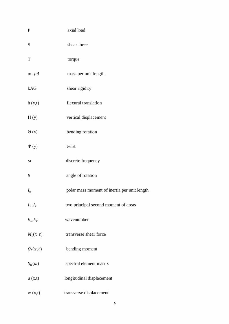
P axial load
S shear force
T torque
m=휌퐴 mass per unit length
kAG shear rigidity
h (y,t) flexural translation
H (y) vertical displacement
Θ (y) bending rotation
Ψ (y) twist
휔 discrete frequency
휃 angle of rotation
퐼 polar mass moment of inertia per unit length
퐼 , 퐼 two principal second moment of areas
푘 ,푘 wavenumber
푀 (푥, 푡) transverse shear force
푄 (푥, 푡) bending moment
푆 (휔) spectral element matrix
u (x,t) longitudinal displacement
w (x,t) transverse displacement
xi
휌 mass density
휑 (y,t) torsional rotation
{u} displacement
{푢̇} velocity
{푢̈} acceleration
1
CHAPTER 1
Introduction
2
1.1 Theoretical Background
1.1.1 Dynamic Stiffness Method (DSM)
The 1941 work by Kolousek is probably the first to derive the dynamic stiffness matrix for
the Bernoulli-Euler beam. Przemieniecki introduced the formulation of the frequency-
dependent mass and stiffness matrices for both bar and beam elements. In contrast to the
conventional finite element mass and stiffness matrices, which results in the linear eigen
problems, the exact dynamic stiffness matrices results in transcendental eigen problems, the
coefficients of which are the transcendental functions of frequency. Thus, a drawback of the
dynamic stiffness method is that it is not an easy task to compute all natural frequencies
accurately by solving the transcendental eigenvalue problems.
In 1971 this difficulty was resolved by Wittrick and Williams by developing by the well-
known Wittrick-Williams algorithm for automatic calculation of undamped natural
frequencies. The exact dynamic stiffness matrix is used in the DSM. The exact dynamic
stiffness matrix is formulated in the frequency domain by using exact dynamic shape
functions that are derived from the exact wave solutions to the governing differential
equations. To obtain the exact wave solutions in the frequency domain, the time-domain
governing differential equations are transformed into the frequency domain by assuming
harmonic solutions of a single frequency. Accordingly the exact dynamic stiffness matrix is
also frequency dependent and it can be considered as a mixture of the inertia, stiffness and
damping properties of a structure element. The dynamic stiffness matrix relates harmonically
varying forces to harmonically varying displacements at the nodes of a structural element.
3
1.1.2 Spectral Analysis Method (SAM)
The solution methods for the governing differential equations formulated in the time-domain
can be categorized into two major groups. The first group consists of the time-domain
methods, such as the numerical integration methods and the modal analysis method, which is
commonly used for the vibration analysis. The second group consists of the frequency-
domain methods. The spectral analysis method (SAM) is one of the frequency–domain
methods.
In SAM, the solutions to the governing differential equations are represented by the
superposition of an infinite number of wave modes of different frequencies. This corresponds
to the continuous Fourier transform of the solutions. This approach involves determining an
infinite set of spectral components in the frequency domain and performing the inverse
Fourier transform to reconstruct the time histories of the solutions. The continuous Fourier
transform is feasible only when the function to be transformed is mathematically simple and
inverse transform is biggest impediment to most practical cases. Instead of using the
continuous Fourier transform, the discrete Fourier transform (DFT) is widely used.
The DFT is an approximation of the continuous Fourier transform. In contrast to the
continuous Fourier transform, the solution is represented by a finite number of wave modes
of discrete frequencies. We can use the fast Fourier transform (FFT) algorithm to compute
the DFT. The use of FFT algorithm make it possible to efficiently take into account as many
spectral components as are needed up to the highest frequency of interest.
1.1.3 Spectral Element Method (SEM)
1. The spectral element method (SEM) can be considered as the combination of the key
features of the conventional FEM, DSM and SAM.
4
2. Key Features of FEM. Meshing and the assembly of finite elements.
3. Key Features of DSM. Exactness of the dynamic stiffness matrix formulated in terms
of a minimum number of DOFs.
4. Key Features of SAM. Superposition of wave modes via DFT theory and FFT
algorithm.
In SEM, exact dynamic stiffness matrices are used as the element stiffness matrices for
the finite element in a structure. To formulate an exact dynamic stiffness matrix for the
classical DSM, the dynamic responses of a structure are usually assumed to be the
harmonic solutions of a single frequency. For the spectral element method (SEM) the
dynamic responses are assumed to be the superposition of a finite number of wave modes
of a different discrete frequencies based on the DFT theory.
The SEM is stiffness formulated. The spectral elements can be assembled to form a
global system matrix equation for the whole problem domain by using exactly the same
assembly techniques as used in the conventional FEM. The global system matrix equation
is then solved for the global spectral nodal DOFs. We use the inverse-FFT (IFFT)
algorithm to compute the time histories of dynamic responses.
1.1.4 Present Scope of Investigation
In the literature many researchers’ have formulated the dynamic stiffness matrix (DSM)
for the vibration problems of rods, beams and frames by using all of the above methods.
They have derived very tedious algebraic expressions by using symbolic computation but
the natural frequencies of the above mentioned structural problems are limited to only the
first few lower mode frequencies. The higher modes natural frequencies of these skeletal
structures are very scanty in literature. Hence in the present thesis the higher modes
natural frequencies up to the twentieth mode are presented for the above structures and
5
the results are compared wherever it was possible. The elements have been spectrally
formulated to obtain the global dynamic stiffness matrix and hence this method is called
spectral element method (SEM).
6
CHAPTER 2
Literature Review
7
Kolousek [35] is the first to derive the dynamic stiffness matrix for the Bernoulli-Euler beam.
Przemieniecki [40] introduced the formulation of the frequency-dependent mass and stiffness
matrices for both bar and beam elements.
The Wittrick-Williams algorithm [47] has enhanced the applicability of the dynamic stiffness
matrix for automatic calculation of undamped natural frequencies.
Beskos [20] introduced the fundamental concept of the spectral element method for the first
time. He derived an exact dynamic stiffness matrix for the beam element and employed FFT
for the dynamic analysis of plane frame-works.
Banerjee, Guo and Howson [10] have presented an exact dynamic stiffness matrix of a
bending-torsion coupled beam including warping. The work presented in this paper extends
the approach by recasting the equations in the form of a dynamic member stiffness matrix. A
new procedure is presented, based on the Wittrick-Willliams algorithm [48] for converging
with certainty upon any required natural frequency.
Banerjee and Williams [12] presented an elegant and efficient alternative procedure for
calculating the number of clamped-clamped natural frequencies of the bending-torsion
coupled beam [13] exceeded by any trial frequency, thus enabling the Wittrick-Williams
algorithm to be applied with ease when finding the natural frequencies of structure which
incorporate such members.
8
The spectral element method is a high-order finite element technique that combines the
geometric flexibility of finite elements with the high accuracy of spectral methods. It exhibits
several favourable computational properties, such as the use of tensor products, naturally
diagonal mass matrices, and adequacy to implementations in a parallel computer system. Due
to these advantages, the spectral element method is a viable alternative to currently popular
methods such as finite volumes and finite elements, if accurate solutions of regular problems
are sought.
Exact dynamic stiffness matrices have been developed mostly for the 1-D structures
including the Timoshenko beams with or without axial force [24, 25, 33, 46], Rayleigh-
Timoshenko beams [3, 36] and composite beams [29].
Banerjee and Williams [15] presented the exact dynamic stiffness matrix for a composite
beam. It includes the effect of shear deformation and rotatory inertia: i.e., it is for a composite
Timoshenko beam. The theory accounts for the coupling between the bending and torsional
deformation which usually occurs for such beams due to anisotropic nature of fibrous
composites.
Chandrashekharaet al. [23] and Abramovich and Livshits [2] considered free bending
vibration of composite Timoshenko beams, but without including the coupling between the
bending and torsional deformations. In contrast, Teoh and Huang [45] and Teh and Huang
[44] included this coupling in their investigation.
9
Abramovich [1] presented the exact solutions for symmetrically laminated composite beams
with ten different boundary conditions, where shear deformation and rotary inertia were
included in the analysis.
Banerjee [5] performed the free vibration analysis of axially loaded composite Timoshenko
beams by using the dynamic stiffness matrix method with the effects of axial force, shear
deformation, rotary inertia and coupling between the bending and the torsional deformations
taken into account.
An exact dynamic stiffness matrix is developed by Banerjee [6] and subsequently used for the
vibration analysis of a twisted beam whose flexural displacement are coupled in two planes.
First the governing differential equations of the motion of the twisted beam undergoing free
natural vibration are derived using Hamilton’s principle. Next the general solution of the
equations are obtained when the oscillatory motion of the beam is harmonic. The resulting
dynamic stiffness matrix is used in connection with the Wittrick-Williams algorithm to
compute natural frequencies and mode shapes of a twisted beam with cantilever end
conditions.
Fiberg [30] has presented an exact dynamic element stiffness matrix which is a coupled one.
An exact dynamic stiffness matrix for a twisted Timoshenko beam has been developed by
Banerjee [8] in order to investigate its free vibration characteristics. First the governing
10
differential equations of motion and the associated natural boundary conditions of a twisted
Timoshenko beam undergoing free natural vibration are derived using Hamilton’s principle.
The inclusion of a given pretwist together with the effects of shear deformation and rotatory
inertia, gives rise in free vibration to four coupled second order partial differential equations
of motion involving bending displacements and bending rotations in two planes. For
harmonic oscillation these four partial differential equations are combined into an eighth
order ordinary differential equation, which is identically satisfied by all components of
bending displacements and bending rotations.
Banerjee and Williams [16] derived exact analytical expressions for coupled extensional-
torsional dynamic stiffness matrix elements of a uniform structural member from the basic
governing differential equation of the member in free vibration.
The spectral element method in structural dynamics was presented by Doyle [27] and he
published [28] in wave propagation in structures where he introduced an FFT-based spectral
analysis methodology. He formulated spectral element for bars, beams and plates using the
spectral analysis of wave motion.
Banerjee and Williams [17] derived the analytical expressions for the coupled bending-
torsional dynamic stiffness matrix element of a uniform Timoshenko beam in an exact sense
by solving the governing differential equations of motion of the element.
11
Banerjee and Fisher [11] have presented analytical expressions for the coupled bending–
torsional dynamic stiffness matrix element of an axially loaded uniform beam.
Banerjee [7] has presented from the governing differential equations of motion in free
vibration, the dynamic stiffness matrix of a uniform rotating Bernoulli–Euler beam using the
Frobenius method of solution in power series. The derivation includes the presence of an
axial force at the outboard end of the beam in addition to the existence of the usual
centrifugal force arising from the rotational motion. This makes the general assembly of
dynamic stiffness matrices of several elements possible so that a non-uniform (or tapered)
rotating beam can be analyzed for its free-vibration characteristics by idealizing it as an
assemblage of many uniform rotating beams.
Gopalakrishnan and Doyle [31] formulated spectral element for beam of varying cross
section to analyse wave propagation in connected waveguides.
Rosen [43] presented the structural and dynamic behaviour of pretwisted rods and beams.
Capron and Williams [21] have presented exact dynamic stiffness coefficients for an axially
loaded Timoshenko member embedded in an elastic medium and shows how to use them in a
general theory for finding the natural frequencies of plane or space frames. The member is
considered to have a uniform distribution of mass and the stiffness’s optionally allow for the
12
separate or combined effects of axial load, rotatory inertia and shear deflection. Axial,
torsional and flexural responses are assumed to be uncoupled, as happens for doubly
symmetric cross-sections.
Banerjee [9] has outlined a general theory to develop the dynamic stiffness matrix of a
structural element. He showed that substantial saving in computer time can be achieved if
explicit analytical expressions for the elements of the dynamic stiffness matrix are used
instead of numerical methods. Such expressions can be derived with the help of symbolic
computation.
Banerjee and Williams [18] in 1985 have used Bernoulli Euler theory and Bessel functions to
obtain explicit expression for the exact stiffness for axial, torsional and flexural deformation
of an axially loaded beam which is tapered.
The coupled bending-torsional dynamic stiffness matrix terms of an axially loaded uniform
Timoshenko beam element are derived by solving the governing differential equations of
motion of the element By Banerjee and Williams [19].
Lee [38] has presented the spectral Element Method and its various applications in the
structural dynamics.
13
Chakraborty and Gopalakrishnan [22] applied spectrally formulated finite element for wave
propagation analysis in functionally graded beams. Howson and Zare [34] formulated an
exact dynamic stiffness matrix for flexural vibration of 3-layered sandwich beams.
Cho and Lee [26] presented An FFT-based spectral analysis method for linear discrete
dynamic systems with non-proportional damping.
Doyle and his collegues [42] have applied the SEM mostly to wave propagation in structures
and a comprehensive list of the works by this group and other researchers can be found in a
book by Doyle [28].
14
CHAPTER 3
Theoretical Formulation
15
3.1 SPECTRAL ELEMENT FORMULATION OF ROD
The free longitudinal vibration of a uniform rod is represented by
EA푢 - ρA푢̈=0 (1)
Where u(x,t) is the longitudinal displacement, E is the Young’s modulus, A is the cross-
sectional area, and ρ is the mass density. The prime denotes the derivatives with respect to the
spatial coordinate x. The internal axial force is given by
푁 (x, t) = EA푢 (x, t) (2)
Where the subscript t is used to denote the quantity in the time domain.
The solution of Equation (1) is assumed in the spectral form as
u (x, t) = eU tin
N
nn
nx ;1
0
(3)
휕 푢휕푥 =
1푁 푒
휕 푈휕푥
휕 푢휕푡 =
1푁 −휔 푒 푈
Substituting Equation (3) into Equation (1) yields eigenvalue problem for a specific discrete
frequency as
EA푈 +휔 휌퐴푈=0 (4)
The general solution to Equation (4) is assumed to be
U (x) = a푒 ( ) (5)
16
= −푘 a푒
By substituting Equation (5) into Equation (4), a dispersion relation can be obtained as
-EA푘 a푒 + 휔 휌퐴a푒 ( ) = 0
- EA푘 + 휔 휌퐴 = 0
푘 -휔 = 0
푘 - 푘 = 0 (6)
Where 푘 is the wavenumber for the pure longitudinal wavemode and it is defined by
푘 = 휔√ (7)
Equation (6) gives two real roots as
푘 = −푘 =푘 (8)
For a finite rod element of length L, the general solution of Equation (4) can be then obtained
in the form
U (x) = 푎 푒−푖푘퐿푥 +푎 푒+푖푘퐿푥 = e (x; 휔) a (9)
where
e (x; 휔) = [푒 푒 ] (10)
a = {푎 푎 }
17
The spectral nodal displacements of the finite rod element can be related to the displacement
field as
d =
UU
2
1 =
)()0(
LUU
(11)
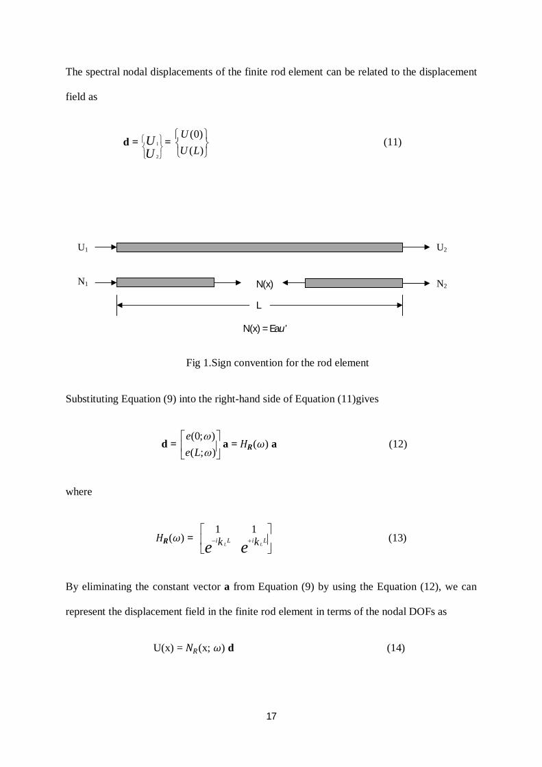
Fig 1.Sign convention for the rod element
Substituting Equation (9) into the right-hand side of Equation (11)gives
d =
);();0(
Lee
a = 퐻푹(휔) a (12)
where
퐻푹(휔) =
ee LiLi kk LL
11
(13)
By eliminating the constant vector a from Equation (9) by using the Equation (12), we can
represent the displacement field in the finite rod element in terms of the nodal DOFs as
U(x) = 푁 (x; 휔) d (14)
U1 U2
N1 N2 N(x)
L
N(x) = Eau’
18
where
푁 (x; 휔) = e(x;휔) 퐻 (휔) = [푁 푁 ]
푁 (푥;휔)=csc (푘 퐿)sin [푘 (퐿 − 푥)] (15)
푁 (푥;휔) = csc (푘 퐿) sin(푘 푥)
From Equation (2), the spectral components of the axial force are related to U(x) by
N(x) = EA푈 (푥) (16)
The spectral nodal axial forces defined for the finite rod element can be related to the forces
defined by the strength of material as
푓 (휔) =
NN
2
1 =
)()0(
LNN
(17)
Substituting Equations (14) and (16) into the right-hand side of Equation (17) gives
푺 (휔) d =풇 (휔) (18)
Where 푺 (휔) is the spectral element matrix for the finite rod element and it is given by
푺 (휔) =
SSSS
RR
RR
2212
1211 = 푺 (휔) (19)
where
푆 = 푆 = (푘 퐿) cot (푘 퐿)
푆 = 푆 = - (푘 퐿) csc (푘 퐿) (20)
19
3.2 SPECTRAL ELEMENT FORMULATION OF EULER-BERNOULLI
BEAM
The free bending vibration of a Bernoulli-beam is represented by
EI푤 +ρA푤̈=0 (1)
Where w (x,t) is the transverse displacement, E is the Young’s modulus, A is the cross-
sectional area, I is the area moment of inertia about the neutral axis, and ρ is the mass density.
The internal transverse shear force and bending moment are given by
Mt (x, t) =EI푤 (x, t), Qt (x, t) = -EI푤 (x, t) (2)
Assuming the solution of equation (1) in the spectral form to be
W (x, t) = eW tin
N
nn
nx ;1
0
(3)
휕 푤휕푥 =
1푁 푒
휕 푊휕푥
휕 푤휕푡 =
1푁 −휔 푒 푊
Substituting Equation (3) into Equation (1) gives an eigenvalue problem for a specific
discrete frequency (휔 = 휔 ) as
퐸퐼푤""+휌퐴푤̈ = 0
퐸퐼푊 ′′′′- 휔 휌퐴푊 = 0 (4)
20
Assuming the general solution of Equation (4)
W(x) = a푒 ( ) (5)
= 푘 a푒
Substituting Equation (5) into Equation (4) yields a dispersion relation,
퐸퐼푊""-휔 휌퐴푊 = 0
퐸퐼(푘 a푒 )-휔 휌퐴(a푒 ( ) ) = 0
퐸퐼(푘 ) -휔 휌퐴 = 0
Then both side divided by EI
푘 -휔 ( ) = 0
푘 - 푘 = 0 (6)
Where푘 is a wavenumber for the pure bending (flexural) wave mode defined by
푘 = √휔/
(7)
Equation (6) gives two pure real roots and two pure imaginary roots as
푘 = 푘 = −푘 , 푘 = 푖푘 = −푘 (8)
For the finite B-beam element of length L, the general solution of the equation (4) can be
obtained in the form
W(x;휔) = 푎 푒 +푎 푒 + 푎 푒 +푎 푒 = e(x;휔) {a} (9)
21
where,
e (x;휔) =[푒 푒 푒 푒 ] (10)
a= {a1 a2 a3 a4}T
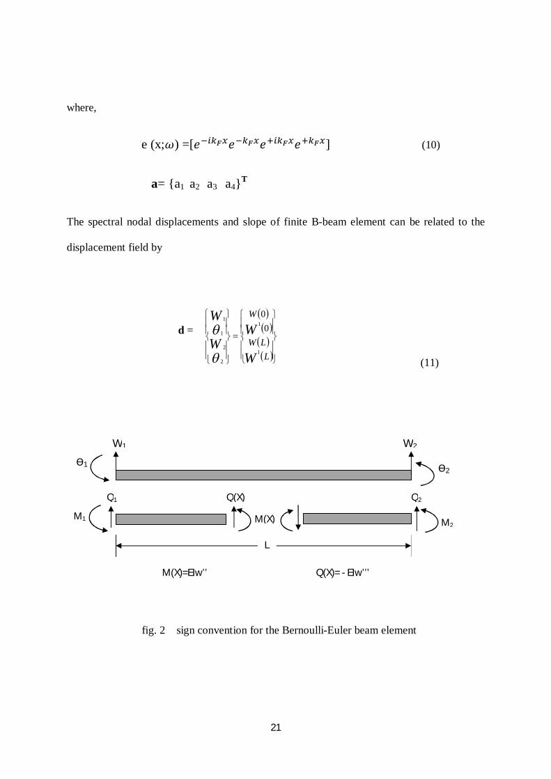
The spectral nodal displacements and slope of finite B-beam element can be related to the
displacement field by
d =
LLW
W
W
WW
W
1
1
2
2
1
1
00
(11)
fig. 2 sign convention for the Bernoulli-Euler beam element
ϴ1 ϴ2
W1 W2
M(X)=EIw’’ Q(X)= - EIw’’’
L
M1 M2
Q1 Q2 Q(X)
M(X)
22
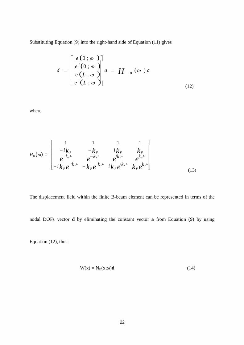
Substituting Equation (9) into the right-hand side of Equation (11) gives
aa
LeLe
ee
d H B )(
;;;0;0
'
'
(12)
where
퐻 (휔) =
ekekekekeeeekkkk
L
F
Li
F
L
F
Li
F
LLiLLiFFFF
kkikki
kkkkii
FFFF
FFFF
1111
(13)
The displacement field within the finite B-beam element can be represented in terms of the
nodal DOFs vector d by eliminating the constant vector a from Equation (9) by using
Equation (12), thus
W(x) = NB(x;ω)d (14)
23
Where
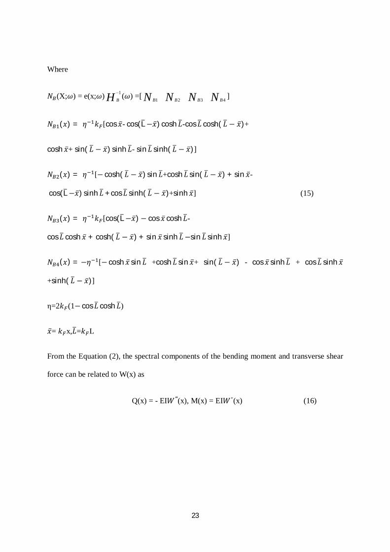
푁 (X;휔) = e(x;휔) H B
1 (휔) =[ NNNN BBBB 4321 ]
푁 (푥) = 휂 푘 [cos 푥̅- cos(L−푥̅) cosh 퐿-cos퐿 cosh( 퐿 − 푥̅)+
cosh 푥̅+ sin( 퐿 − 푥̅) sinh 퐿- sin 퐿 sinh( 퐿 − 푥̅)]
푁 (푥) = 휂 [− cosh( 퐿 − 푥̅) sin 퐿+cosh 퐿 sin( 퐿 − 푥̅) + sin 푥̅-
cos(L−푥̅) sinh 퐿+cos퐿 sinh( 퐿 − 푥̅)+sinh 푥̅] (15)
푁 (푥) = 휂 푘 [cos(L−푥̅)− cos 푥̅ cosh 퐿-
cos퐿 cosh 푥̅ + cosh( 퐿 − 푥̅) + sin 푥̅ sinh 퐿−sin 퐿 sinh 푥̅]
푁 (푥) = −휂 [− cosh 푥̅ sin 퐿 +cosh 퐿 sin 푥̅+ sin( 퐿 − 푥̅) - cos 푥̅ sinh 퐿 + cos 퐿 sinh 푥̅
+sinh( 퐿 − 푥̅)]
η=2푘 (1− cos퐿 cosh 퐿)
푥̅= 푘 x,퐿=푘 L
From the Equation (2), the spectral components of the bending moment and transverse shear
force can be related to W(x) as
Q(x) = - EI푊‴(x), M(x) = EI푊״(x) (16)
24
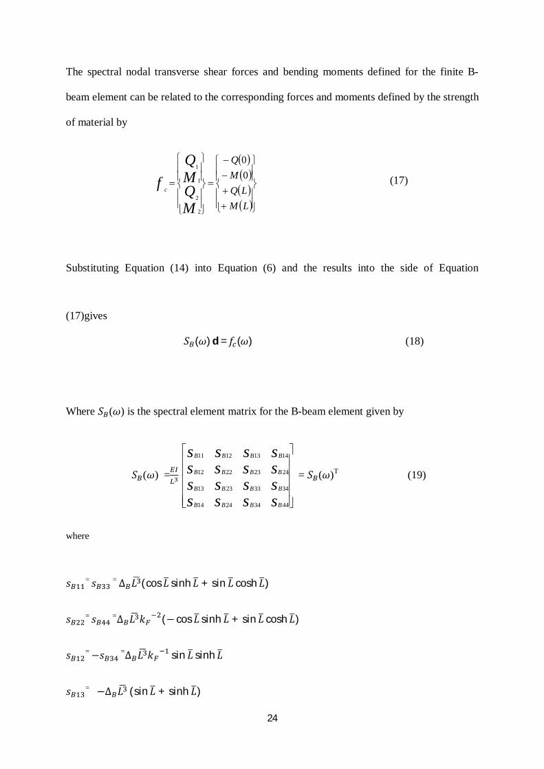
The spectral nodal transverse shear forces and bending moments defined for the finite B-
beam element can be related to the corresponding forces and moments defined by the strength
of material by
LMLQ
MQ
MQMQ
f c
00
2
2
1
1
(17)
Substituting Equation (14) into Equation (6) and the results into the side of Equation
(17)gives
푆 (휔) d = 푓 (휔) (18)
Where 푆 (휔) is the spectral element matrix for the B-beam element given by
푆 (휔) =
ssssssssssssssss
BBBB
BBBB
BBBB
BBBB
44342414
34332313
24232212
14131211
= 푆 (휔)T (19)
where
푠 = 푠 = ∆ 퐿 (cos퐿 sinh 퐿 + sin 퐿 cosh 퐿)
푠 = 푠 =∆ 퐿 푘 (− cos 퐿 sinh 퐿 + sin 퐿 cosh 퐿)
푠 = −푠 =∆ 퐿 푘 sin 퐿 sinh 퐿
푠 = −∆ 퐿 (sin 퐿 + sinh 퐿)
25
푠 = −푠 =∆ 퐿 푘 (− cos 퐿 + cosh 퐿)
푠 = ∆ 퐿 푘 (−sin 퐿 + sinh 퐿)(20)
∆ =
퐿=푘 L
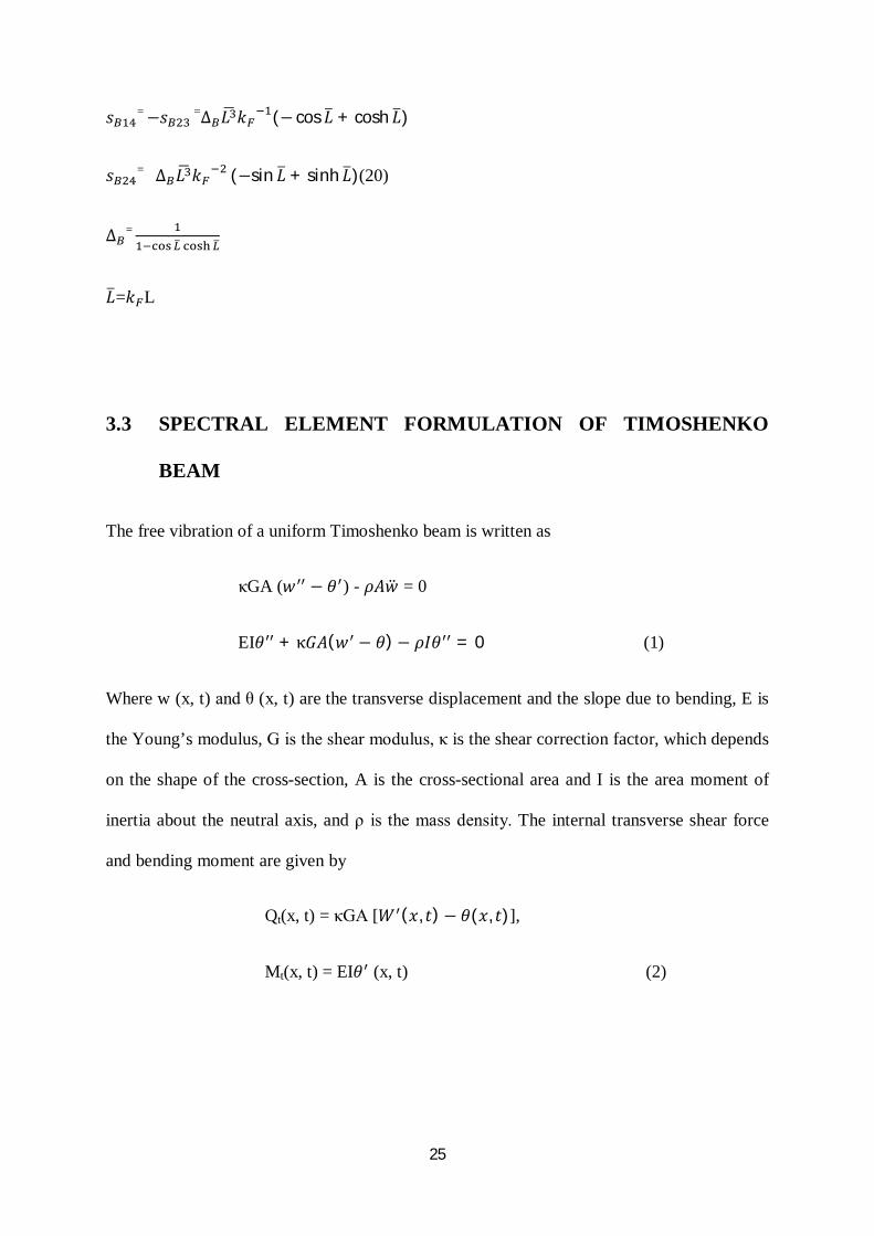
3.3 SPECTRAL ELEMENT FORMULATION OF TIMOSHENKO
BEAM
The free vibration of a uniform Timoshenko beam is written as
κGA (푤 − 휃 ) - 휌퐴푤̈ = 0
EI휃 + κ퐺퐴(푤 − 휃) − 휌퐼휃 = 0 (1)
Where w (x, t) and θ (x, t) are the transverse displacement and the slope due to bending, E is
the Young’s modulus, G is the shear modulus, κ is the shear correction factor, which depends
on the shape of the cross-section, A is the cross-sectional area and I is the area moment of
inertia about the neutral axis, and ρ is the mass density. The internal transverse shear force
and bending moment are given by
Qt(x, t) = κGA [푊 (푥, 푡) − 휃(푥, 푡)],
Mt(x, t) = EI휃 (x, t) (2)
26
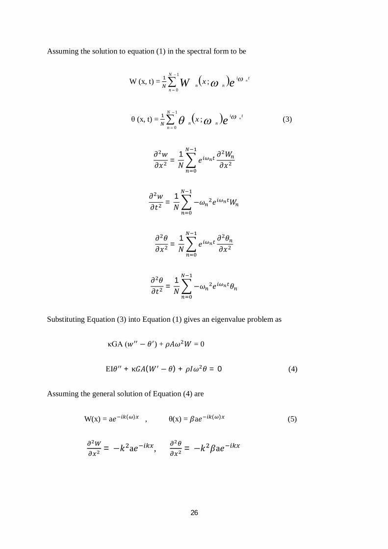
Assuming the solution to equation (1) in the spectral form to be
W (x, t) = eW tin
N
nn
nx ;1
0
θ (x, t) = e tin
N
nn
nx ;1
0
(3)
휕 푤휕푥 =
1푁 푒
휕 푊휕푥
휕 푤휕푡 =
1푁 −휔 푒 푊
휕 휃휕푥 =
1푁 푒
휕 휃휕푥
휕 휃휕푡 =
1푁 −휔 푒 휃
Substituting Equation (3) into Equation (1) gives an eigenvalue problem as
κGA (푤 − 휃 ) + 휌퐴휔 푊 = 0
EI휃 + κ퐺퐴(푊 − 휃) + 휌퐼휔 휃 = 0 (4)
Assuming the general solution of Equation (4) are
W(x) = a푒 ( ) , θ(x) = 훽a푒 ( ) (5)
= −푘 a푒 , = −푘 훽a푒
27
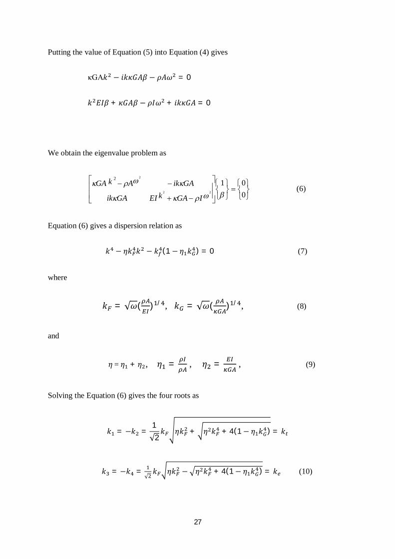
Putting the value of Equation (5) into Equation (4) gives
κGA푘 − 푖푘휅퐺퐴훽 − 휌퐴휔 = 0
푘 퐸퐼훽 + 휅퐺퐴훽 − 휌퐼휔 + 푖푘휅퐺퐴 = 0
We obtain the eigenvalue problem as
001
22
22
IGAkEIGAik
GAikAkGA (6)
Equation (6) gives a dispersion relation as
푘 − 휂푘 푘 − 푘 (1 − 휂 푘 ) = 0 (7)
where
푘 = √휔( ) / , 푘 = √휔( ) / , (8)
and
휂 = 휂 + 휂 , 휂 = , 휂 = , (9)
Solving the Equation (6) gives the four roots as
푘 = −푘 =1√2
푘 휂푘 + 휂 푘 + 4(1− 휂 푘 ) = 푘
푘 = −푘 =√푘 휂푘 − 휂 푘 + 4(1− 휂 푘 ) = 푘 (10)
28
훽 =휅퐺퐴푘 − 휌퐴휔
푖푘휅퐺퐴
= (푘 − 푘 )
From the Equation (6), we can obtain the wave mode ratio as
훽 (휔) =1푖푘
(푘 − 푘 )
= - i푟 (휔) (11)
where
푟 (휔) = (푘 − 푘 ) (12)
By using the four wave numbers, the general solution of Equations (4) can be written as
W (x) = 푎 푒 +푎 푒 + 푎 푒 +푎 푒 = 푒 (x;휔) {a} (13)
Θ (x) = 훽 푎 푒 +훽 푎 푒 + 훽 푎 푒 +훽 푎 푒 = 푒 (x;휔) {a} (14)
where
a = {a1 a2 a3 a4}T (15)
e (x; 휔) = [푒 푒 푒 푒 ] (16)
e (x; 휔) = e (x; 휔) B (휔)
B (휔) = diag [β (ω)]
29
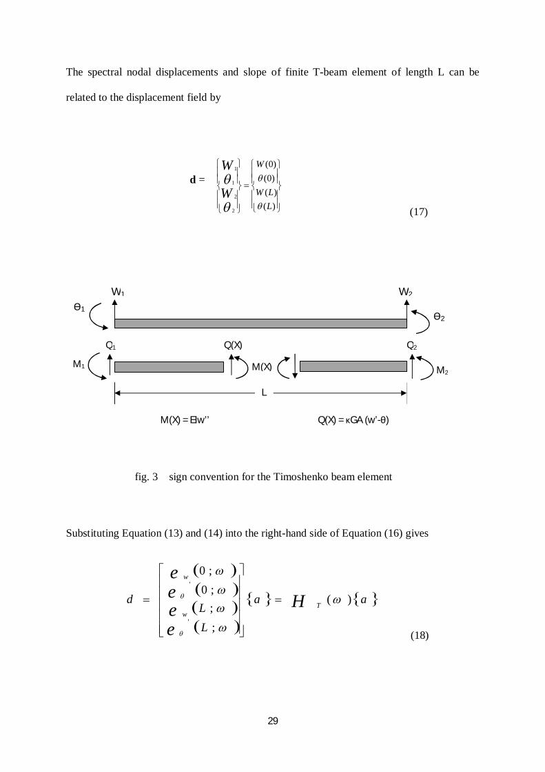
The spectral nodal displacements and slope of finite T-beam element of length L can be
related to the displacement field by
d =
)()()0()0(
2
2
1
1
LLW
W
W
W
(17)
fig. 3 sign convention for the Timoshenko beam element
Substituting Equation (13) and (14) into the right-hand side of Equation (16) gives
aa
LL
d Heeee
Tw
w
)(
;;;0;0
'
'
(18)
ϴ1ϴ2
W1 W2
M(X) = EIw’’ Q(X) = κGA (w’-θ)
L
M1 M2
Q1 Q2 Q(X)
M(X)
30
where
퐻 (휔) =
eirererereeeeirrrr
eeeetttt
eett
eett
iii
iii
11
11
1111
(19)
Where
e = e , e = e ,
푟 = (푘 − 푘 ), 푟 = (푘 − 푘 )
By using Equation (18), the constant vector a can be eliminated from Equation (13) and (14)
to express the general solutions as
W (x) = 푁 (x; 휔) d, θ (x) = 푁 (x; 휔) d, (20)
Where
푁 (x; 휔) = e (x;ω)H (ω)
푁 (x; 휔) = e (x;ω)H (ω) = e (x;ω)B(ω)H (ω) (21)
From the Equation (2), the spectral components of the bending moment and transverse shear
force can be related to W(x) and θ(x) as
Q = κGA(푊 − 휃), M = EI휃 (22)
31
The spectral nodal transverse shear forces and bending moments defined for the finite T-
beam element can be related to the corresponding forces and moments defined by the strength
of material by
LMLQ
MQ
MQMQ
f c
00
)(
2
2
1
1
(23)
Substituting Equation (20) into Equation (22) and the results to the right-side of Equation
(23) gives
푆 (휔) d = 푓 (휔) (24)
Where 푆 (휔) is the spectral element matrix for the T-beam is given by
푆 (휔) =퐸퐼
ssssssssssssssss
TTTT
TTTT
TTTT
TTTT
44342414
34332313
24232212
14131211
= 푆 (휔)T (25)
where
푠 = 푠 = 푖∆ A[(e − 1)(e + 1)r − (e + 1)(e − 1)r ](k r − k r )
푠 = 푠 = ∆ B[−(e + 1)(e − 1)r + (e − 1)(e + 1)r ]
푠 = −푠 = ∆ 퐴{(e − 1)(e − 1)(k r + k r ) − [(e + 1)(e + 1)− 4e e ](k r
− k r ) }
32
푠 = 2푖∆ 퐴[(e − 1)e r − (e − 1)e r ](−k r + k r )
푠 = −푠 = −2∆ 퐴(e − e )(1− e e )(−k r + k r )
푠 = 2∆ 퐵[(e − 1)e r − (e − 1)e r ]
∆ =
[ {(et2+1)(ee
2+1) etee} (rt2+re
2)(et2−1)(ee
2−1)]
퐴 = (1 8⁄ )푒 (1− 휂 푘퐺4 ) /
퐵 = (1 8⁄ )푒 [휂 푘퐹4 + 4 1 − 휂 푘퐺
4 ] /
3.4 SPECTRAL ELEMENT FORMULATION OF FRAME
The differential equation of the frame may be written as
EI + m = 0 (1)
where y(t) is the deflection at point x from origin, EI is the flexural rigidity, m is the mass
per unit length.
Assuming the solution of the equation (1) in the spectral form to be
Y(x, t) = eY tin
N
nn
nx ;1
0
(2)
휕 푦휕푥 =
1푁 푒
휕 푌휕푥
휕 푦휕푡 =
1푁 −휔 푒 푌
Putting the above value in equation (1), get the solution as
33
퐸퐼푌""-휔 푚푌 = 0 (3)
Assuming the general solution for equation (3)
Y(x) = a푒 ( ) (4)
휕 푦휕푥 = 푘 푎푒−푖푘푥
The general solution of the equation (3) can be obtained in the form
Y(x;휔) = 푎 푒 +푎 푒 + 푎 푒 +푎 푒 (5)
The equation (5) can be written in the form
Y= 퐶 cosh 휆 + 퐶 sinh 휆 + 퐶 cos휆 + 퐶 sin 휆 (6)
where Y is the amplitude of motion,
λ = ( )퐿
휔 = circular frequency of vibration
and the constants 퐶 ,퐶 ,퐶 ,퐶 are dependent on the boundary conditions.
34
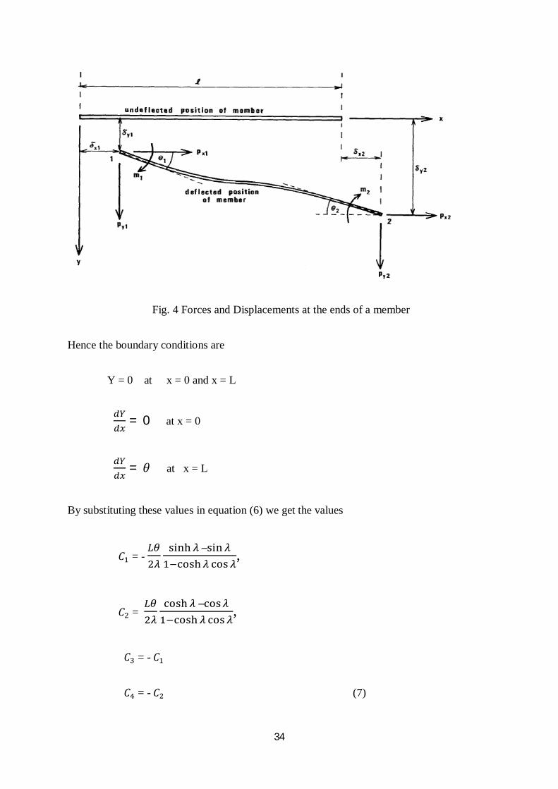
Fig. 4 Forces and Displacements at the ends of a member
Hence the boundary conditions are
Y = 0 at x = 0 and x = L
= 0 at x = 0
= 휃 at x = L
By substituting these values in equation (6) we get the values
퐶 = - – ,
퐶 = – ,
퐶 = - 퐶
퐶 = - 퐶 (7)
35
Putting the values of 퐶 ,퐶 ,퐶 ,퐶 in equation (6) we get the values
S = λ ( ), (8)
C = , (9)
Q = 휆 ( ), (10)
q = , (11)
where
S is the dynamic flexural stiffness,
C is the dynamic flexural carry-over factor,
Q is the dynamic flexural shear stiffness,
q is the dynamic flexure-shear carry-over factor,
K is the ‘’stiffness’’ of the member,
Where 휆 = 휇휔 푙 퐸퐼⁄ and 휇 is the mass per unit length of the member
36
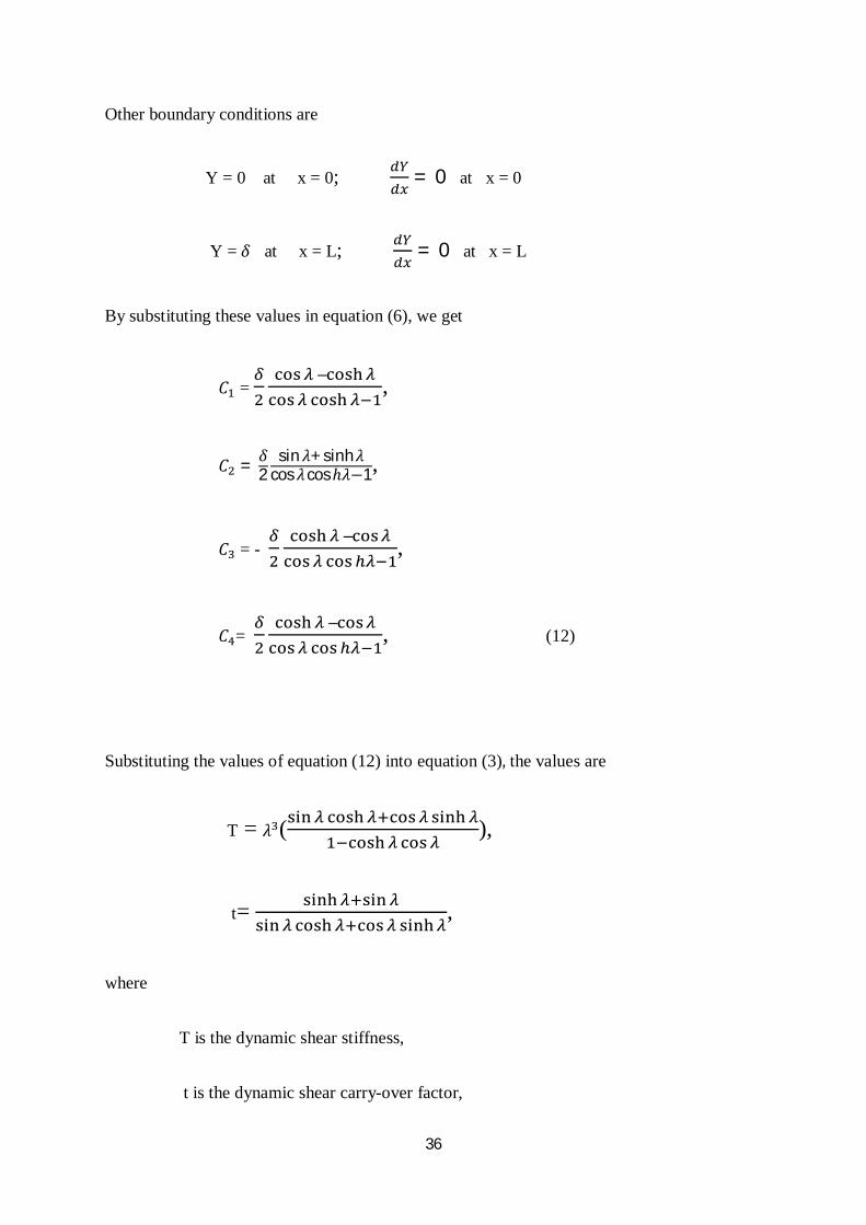
Other boundary conditions are
Y = 0 at x = 0; = 0 at x = 0
Y = 훿 at x = L; = 0 at x = L
By substituting these values in equation (6), we get
퐶 = – ,
퐶 = 훿2
sin휆+sinh휆cos휆cosℎ휆−1,
퐶 = - – ,
퐶 = – , (12)
Substituting the values of equation (12) into equation (3), the values are
T = 휆 ( ),
t= ,
where
T is the dynamic shear stiffness,
t is the dynamic shear carry-over factor,
37
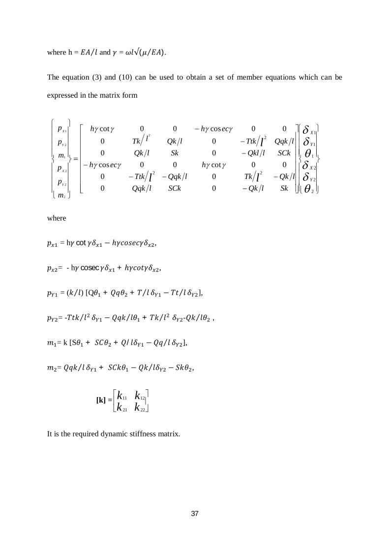
where h = 퐸퐴 푙⁄ and 훾 = 휔푙√(휇 퐸퐴⁄ ).
The equation (3) and (10) can be used to obtain a set of member equations which can be
expressed in the matrix form
where
푝 = h훾 cot 훾훿 − ℎ훾푐표푠푒푐훾훿 ,
푝 = - h훾 cosec 훾훿 + ℎ훾푐표푡훾훿 ,
푝 = (푘 푙⁄ ) [Q휃 + 푄푞휃 + 푇 푙⁄ 훿 − 푇푡 푙⁄ 훿 ],
푝 = -푇푡푘 푙⁄ 훿 − 푄푞푘 푙휃 + 푇푘 푙 ⁄⁄ 훿 -푄푘 푙휃⁄ ,
푚 = k [S휃 + 푆퐶휃 + 푄/푙훿 − 푄푞 푙⁄ 훿 ],
푚 = 푄푞푘 푙⁄ 훿 + 푆퐶푘휃 − 푄푘 푙훿⁄ − 푆푘휃 ,
[k] =
kkkk
2221
1211
It is the required dynamic stiffness matrix.
2
2
2
1
1
1
22
2
0000
00cot00cos0000
00cos00cot2
2
2
2
1
2
1
Y
X
Y
X
SklQkSCklQqklQkTklQqkTtk
hechSCklQklSklQk
lQqkTtklQklTkechh
m
p
pm
p
p
ll
l
Y
X
Y
X
38
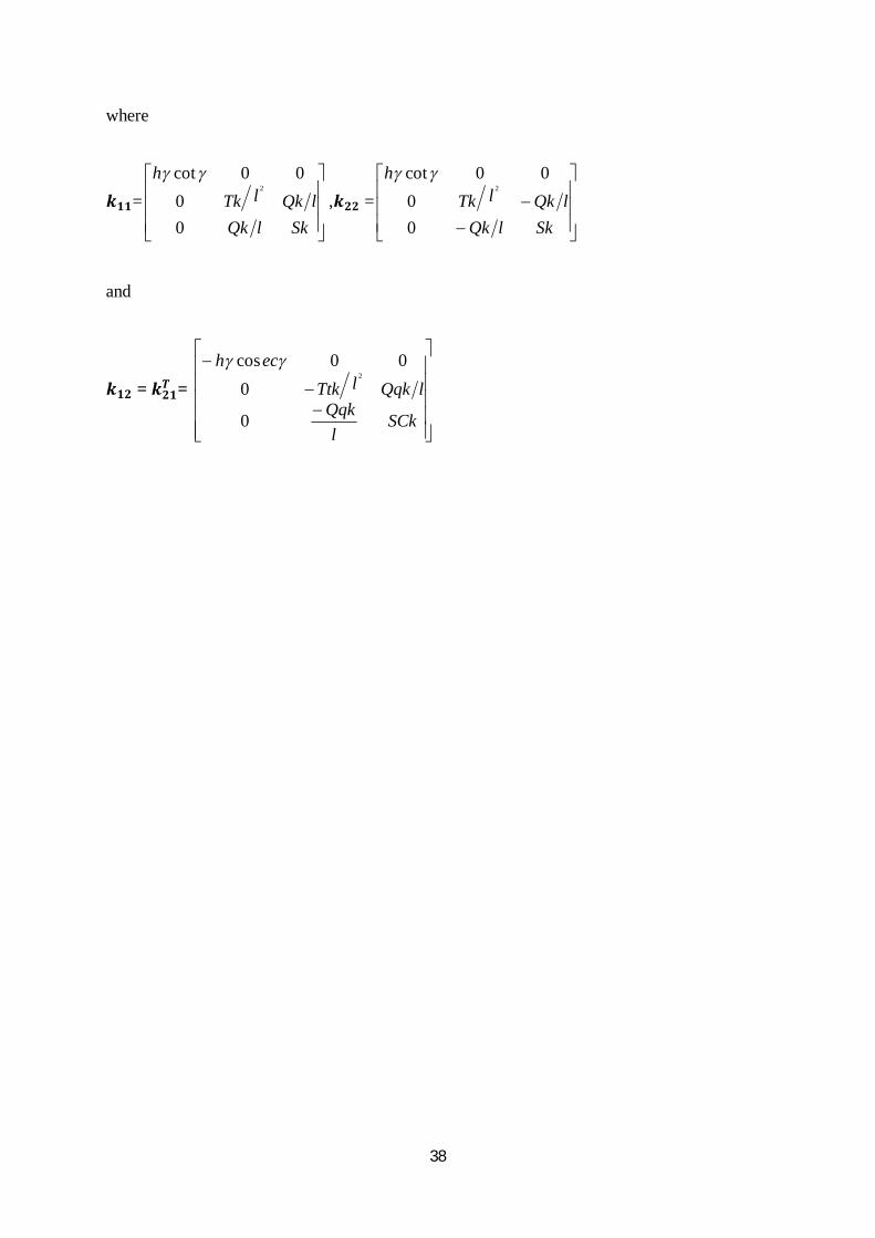
where
풌ퟏퟏ=
SklQklQklTk
h
00
00cot2
,풌ퟐퟐ =
SklQklQklTk
h
00
00cot2
and
풌ퟏퟐ = 풌ퟐퟏ푻 =
SCkl
QqklQqklTtk
ech
0
000cos
2
39
CHAPTER 4
Results and Discussions
40
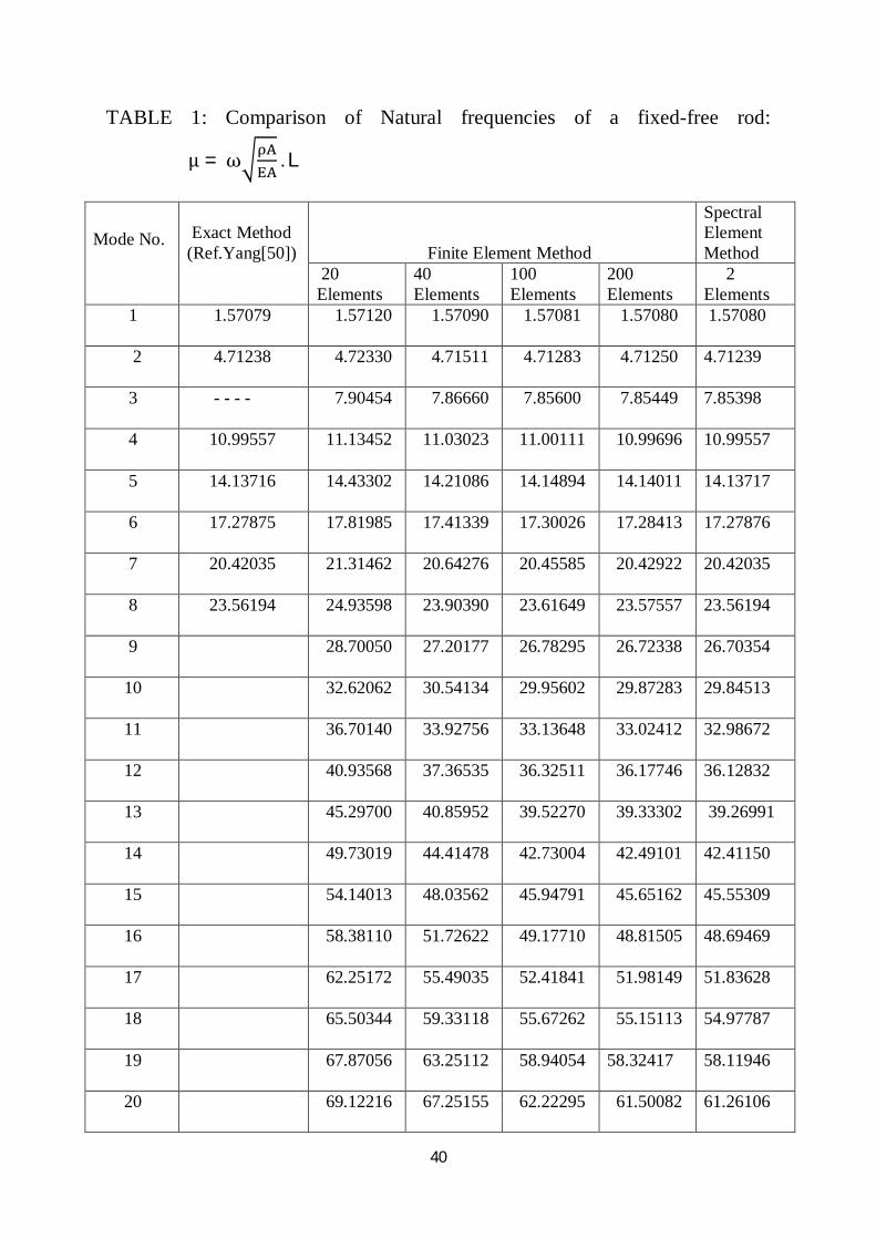
TABLE 1: Comparison of Natural frequencies of a fixed-free rod:
μ = ω . L
Mode No.
Exact Method (Ref.Yang[50])
Finite Element Method
Spectral Element Method
20 Elements
40 Elements
100 Elements
200 Elements
2 Elements
1 1.57079 1.57120 1.57090 1.57081 1.57080 1.57080
2 4.71238 4.72330 4.71511 4.71283 4.71250 4.71239
3 - - - - 7.90454 7.86660 7.85600 7.85449 7.85398
4 10.99557 11.13452 11.03023 11.00111 10.99696 10.99557
5 14.13716 14.43302 14.21086 14.14894 14.14011 14.13717
6 17.27875 17.81985 17.41339 17.30026 17.28413 17.27876
7 20.42035 21.31462 20.64276 20.45585 20.42922 20.42035
8 23.56194 24.93598 23.90390 23.61649 23.57557 23.56194
9 28.70050 27.20177 26.78295 26.72338 26.70354
10 32.62062 30.54134 29.95602 29.87283 29.84513
11 36.70140 33.92756 33.13648 33.02412 32.98672
12 40.93568 37.36535 36.32511 36.17746 36.12832
13 45.29700 40.85952 39.52270 39.33302 39.26991
14 49.73019 44.41478 42.73004 42.49101 42.41150
15 54.14013 48.03562 45.94791 45.65162 45.55309
16 58.38110 51.72622 49.17710 48.81505 48.69469
17 62.25172 55.49035 52.41841 51.98149 51.83628
18 65.50344 59.33118 55.67262 55.15113 54.97787
19 67.87056 63.25112 58.94054 58.32417 58.11946
20 69.12216 67.25155 62.22295 61.50082 61.26106
41
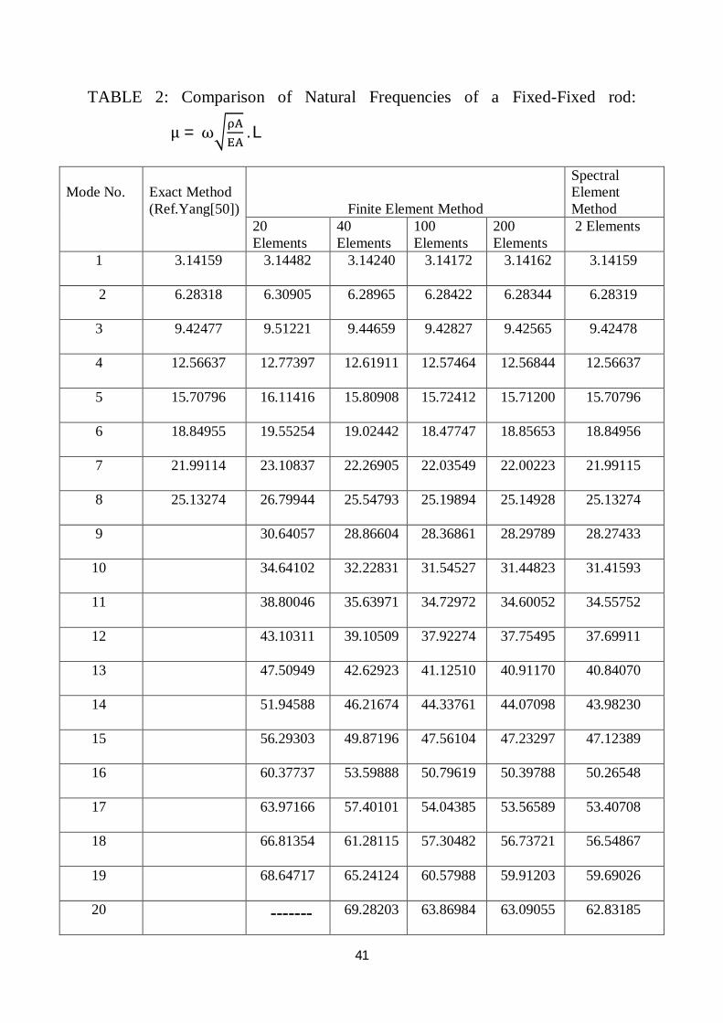
TABLE 2: Comparison of Natural Frequencies of a Fixed-Fixed rod:
μ = ω . L
Mode No.
Exact Method (Ref.Yang[50])
Finite Element Method
Spectral Element Method
20 Elements
40 Elements
100 Elements
200 Elements
2 Elements
1 3.14159 3.14482 3.14240 3.14172 3.14162 3.14159
2 6.28318 6.30905 6.28965 6.28422 6.28344 6.28319
3 9.42477 9.51221 9.44659 9.42827 9.42565 9.42478
4 12.56637 12.77397 12.61911 12.57464 12.56844 12.56637
5 15.70796 16.11416 15.80908 15.72412 15.71200 15.70796
6 18.84955 19.55254 19.02442 18.47747 18.85653 18.84956
7 21.99114 23.10837 22.26905 22.03549 22.00223 21.99115
8 25.13274 26.79944 25.54793 25.19894 25.14928 25.13274
9 30.64057 28.86604 28.36861 28.29789 28.27433
10 34.64102 32.22831 31.54527 31.44823 31.41593
11 38.80046 35.63971 34.72972 34.60052 34.55752
12 43.10311 39.10509 37.92274 37.75495 37.69911
13 47.50949 42.62923 41.12510 40.91170 40.84070
14 51.94588 46.21674 44.33761 44.07098 43.98230
15 56.29303 49.87196 47.56104 47.23297 47.12389
16 60.37737 53.59888 50.79619 50.39788 50.26548
17 63.97166 57.40101 54.04385 53.56589 53.40708
18 66.81354 61.28115 57.30482 56.73721 56.54867
19 68.64717 65.24124 60.57988 59.91203 59.69026
20 ------- 69.28203 63.86984 63.09055 62.83185
42
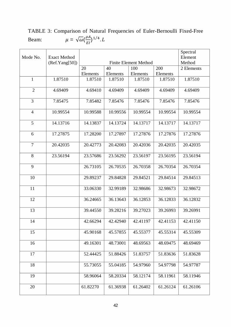
TABLE 3: Comparison of Natural Frequencies of Euler-Bernoulli Fixed-Free Beam: 휇 = √휔( ) ⁄ .퐿
Mode No.
Exact Method (Ref.Yang[50])
Finite Element Method
Spectral Element Method
20 Elements
40 Elements
100 Elements
200 Elements
2 Elements
1 1.87510 1.87510 1.87510 1.87510 1.87510 1.87510
2 4.69409 4.69410 4.69409 4.69409 4.69409 4.69409
3 7.85475 7.85482 7.85476 7.85476 7.85476 7.85476
4 10.99554 10.99588 10.99556 10.99554 10.99554 10.99554
5 14.13716 14.13837 14.13724 14.13717 14.13717 14.13717
6 17.27875 17.28200 17.27897 17.27876 17.27876 17.27876
7 20.42035 20.42773 20.42083 20.42036 20.42035 20.42035
8 23.56194 23.57686 23.56292 23.56197 23.56195 23.56194
9 26.73105 26.70535 26.70358 26.70354 26.70354
10 29.89237 29.84828 29.84521 29.84514 29.84513
11 33.06330 32.99189 32.98686 32.98673 32.98672
12 36.24665 36.13643 36.12853 36.12833 36.12832
13 39.44550 39.28216 39.27023 39.26993 39.26991
14 42.66294 42.42940 42.41197 42.41153 42.41150
15 45.90168 45.57855 45.55377 45.55314 45.55309
16 49.16301 48.73001 48.69563 48.69475 48.69469
17 52.44425 51.88426 51.83757 51.83636 51.83628
18 55.73055 55.04185 54.97960 54.97798 54.97787
19 58.96064 58.20334 58.12174 58.11961 58.11946
20 61.82270 61.36938 61.26402 61.26124 61.26106
43
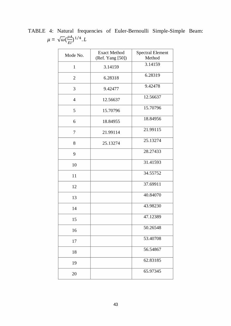
TABLE 4: Natural frequencies of Euler-Bernoulli Simple-Simple Beam: 휇 = √휔( ) ⁄ . 퐿
Mode No. Exact Method (Ref. Yang [50])
Spectral Element Method
1 3.14159 3.14159
2 6.28318 6.28319
3 9.42477 9.42478
4 12.56637 12.56637
5 15.70796 15.70796
6 18.84955 18.84956
7 21.99114 21.99115
8 25.13274 25.13274
9 28.27433
10 31.41593
11 34.55752
12 37.69911
13 40.84070
14 43.98230
15 47.12389
16 50.26548
17 53.40708
18 56.54867
19 62.83185
20 65.97345
44
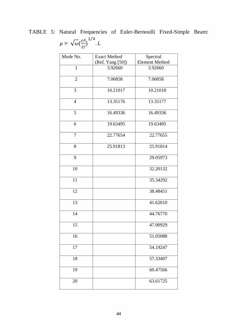
TABLE 5: Natural Frequencies of Euler-Bernoulli Fixed-Simple Beam:
휇 = √휔(휌퐴
퐸퐼)
1 4⁄. 퐿
Mode No. Exact Method (Ref. Yang [50])
Spectral Element Method
1 3.92660 3.92660
2 7.06858 7.06858
3 10.21017 10.21018
4 13.35176 13.35177
5 16.49336 16.49336
6 19.63495 19.63495
7 22.77654 22.77655
8 25.91813 25.91814
9 29.05973
10 32.20132
11 35.34292
12 38.48451
13 41.62610
14 44.76770
15 47.90929
16 51.05088
17 54.19247
18 57.33407
19 60.47566
20 63.61725
45
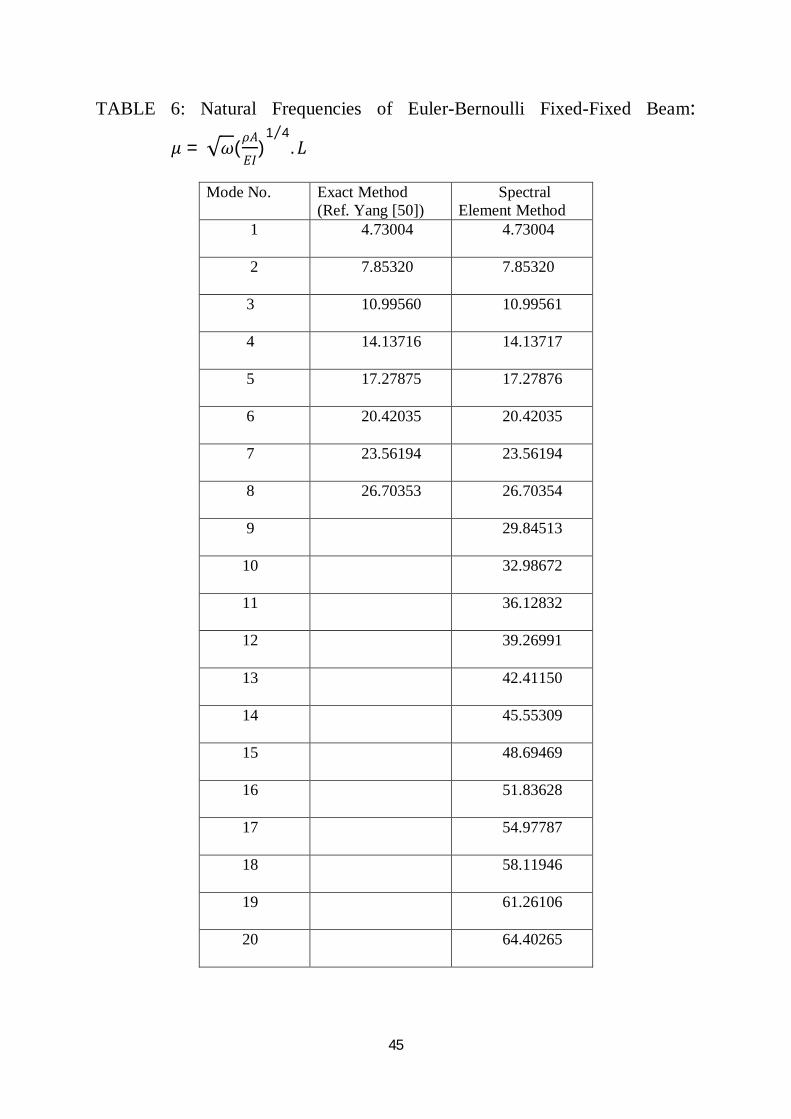
TABLE 6: Natural Frequencies of Euler-Bernoulli Fixed-Fixed Beam:
휇 = √휔(휌퐴
퐸퐼)
1 4⁄. 퐿
Mode No. Exact Method (Ref. Yang [50])
Spectral Element Method
1 4.73004 4.73004
2 7.85320 7.85320
3 10.99560 10.99561
4 14.13716 14.13717
5 17.27875 17.27876
6 20.42035 20.42035
7 23.56194 23.56194
8 26.70353 26.70354
9 29.84513
10 32.98672
11 36.12832
12 39.26991
13 42.41150
14 45.55309
15 48.69469
16 51.83628
17 54.97787
18 58.11946
19 61.26106
20 64.40265
46
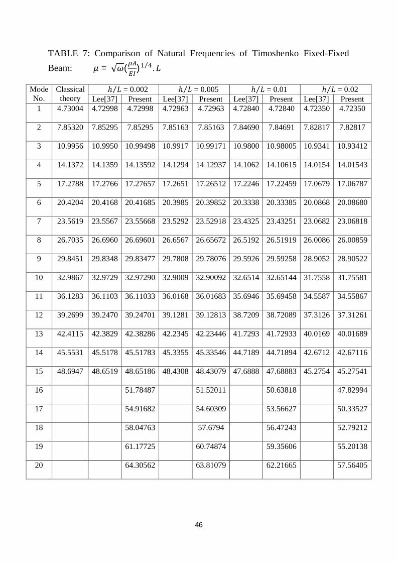
TABLE 7: Comparison of Natural Frequencies of Timoshenko Fixed-Fixed Beam: 휇 = √휔( ) ⁄ . 퐿
Mode No.
Classical theory
ℎ 퐿⁄ = 0.002 ℎ 퐿⁄ = 0.005 ℎ 퐿⁄ = 0.01 ℎ 퐿⁄ = 0.02 Lee[37] Present Lee[37] Present Lee[37] Present Lee[37] Present
1 4.73004 4.72998 4.72998 4.72963 4.72963 4.72840 4.72840 4.72350 4.72350
2 7.85320 7.85295 7.85295 7.85163 7.85163 7.84690 7.84691 7.82817 7.82817
3 10.9956 10.9950 10.99498 10.9917 10.99171 10.9800 10.98005 10.9341 10.93412
4 14.1372 14.1359 14.13592 14.1294 14.12937 14.1062 14.10615 14.0154 14.01543
5 17.2788 17.2766 17.27657 17.2651 17.26512 17.2246 17.22459 17.0679 17.06787
6 20.4204 20.4168 20.41685 20.3985 20.39852 20.3338 20.33385 20.0868 20.08680
7 23.5619 23.5567 23.55668 23.5292 23.52918 23.4325 23.43251 23.0682 23.06818
8 26.7035 26.6960 26.69601 26.6567 26.65672 26.5192 26.51919 26.0086 26.00859
9 29.8451 29.8348 29.83477 29.7808 29.78076 29.5926 29.59258 28.9052 28.90522
10 32.9867 32.9729 32.97290 32.9009 32.90092 32.6514 32.65144 31.7558 31.75581
11 36.1283 36.1103 36.11033 36.0168 36.01683 35.6946 35.69458 34.5587 34.55867
12 39.2699 39.2470 39.24701 39.1281 39.12813 38.7209 38.72089 37.3126 37.31261
13 42.4115 42.3829 42.38286 42.2345 42.23446 41.7293 41.72933 40.0169 40.01689
14 45.5531 45.5178 45.51783 45.3355 45.33546 44.7189 44.71894 42.6712 42.67116
15 48.6947 48.6519 48.65186 48.4308 48.43079 47.6888 47.68883 45.2754 45.27541
16 51.78487 51.52011 50.63818 47.82994
17 54.91682 54.60309 53.56627 50.33527
18 58.04763 57.6794 56.47243 52.79212
19 61.17725 60.74874 59.35606 55.20138
20 64.30562 63.81079 62.21665 57.56405
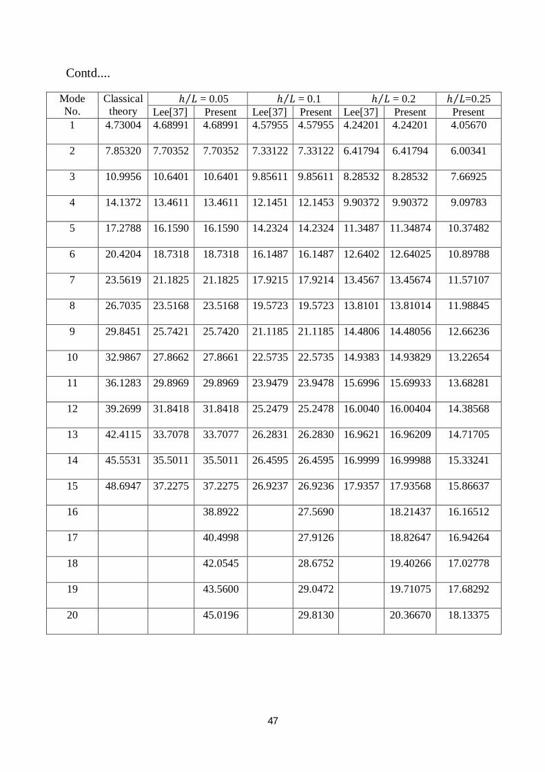
47
Contd....
Mode No.
Classical theory
ℎ 퐿⁄ = 0.05 ℎ 퐿⁄ = 0.1 ℎ 퐿⁄ = 0.2 ℎ 퐿⁄ =0.25 Lee[37] Present Lee[37] Present Lee[37] Present Present
1 4.73004 4.68991 4.68991 4.57955 4.57955 4.24201 4.24201 4.05670
2 7.85320 7.70352 7.70352 7.33122 7.33122 6.41794 6.41794 6.00341
3 10.9956 10.6401 10.6401 9.85611 9.85611 8.28532 8.28532 7.66925
4 14.1372 13.4611 13.4611 12.1451 12.1453 9.90372 9.90372 9.09783
5 17.2788 16.1590 16.1590 14.2324 14.2324 11.3487 11.34874 10.37482
6 20.4204 18.7318 18.7318 16.1487 16.1487 12.6402 12.64025 10.89788
7 23.5619 21.1825 21.1825 17.9215 17.9214 13.4567 13.45674 11.57107
8 26.7035 23.5168 23.5168 19.5723 19.5723 13.8101 13.81014 11.98845
9 29.8451 25.7421 25.7420 21.1185 21.1185 14.4806 14.48056 12.66236
10 32.9867 27.8662 27.8661 22.5735 22.5735 14.9383 14.93829 13.22654
11 36.1283 29.8969 29.8969 23.9479 23.9478 15.6996 15.69933 13.68281
12 39.2699 31.8418 31.8418 25.2479 25.2478 16.0040 16.00404 14.38568
13 42.4115 33.7078 33.7077 26.2831 26.2830 16.9621 16.96209 14.71705
14 45.5531 35.5011 35.5011 26.4595 26.4595 16.9999 16.99988 15.33241
15 48.6947 37.2275 37.2275 26.9237 26.9236 17.9357 17.93568 15.86637
16 38.8922 27.5690 18.21437 16.16512
17 40.4998 27.9126 18.82647 16.94264
18 42.0545 28.6752 19.40266 17.02778
19 43.5600 29.0472 19.71075 17.68292
20 45.0196 29.8130 20.36670 18.13375
48
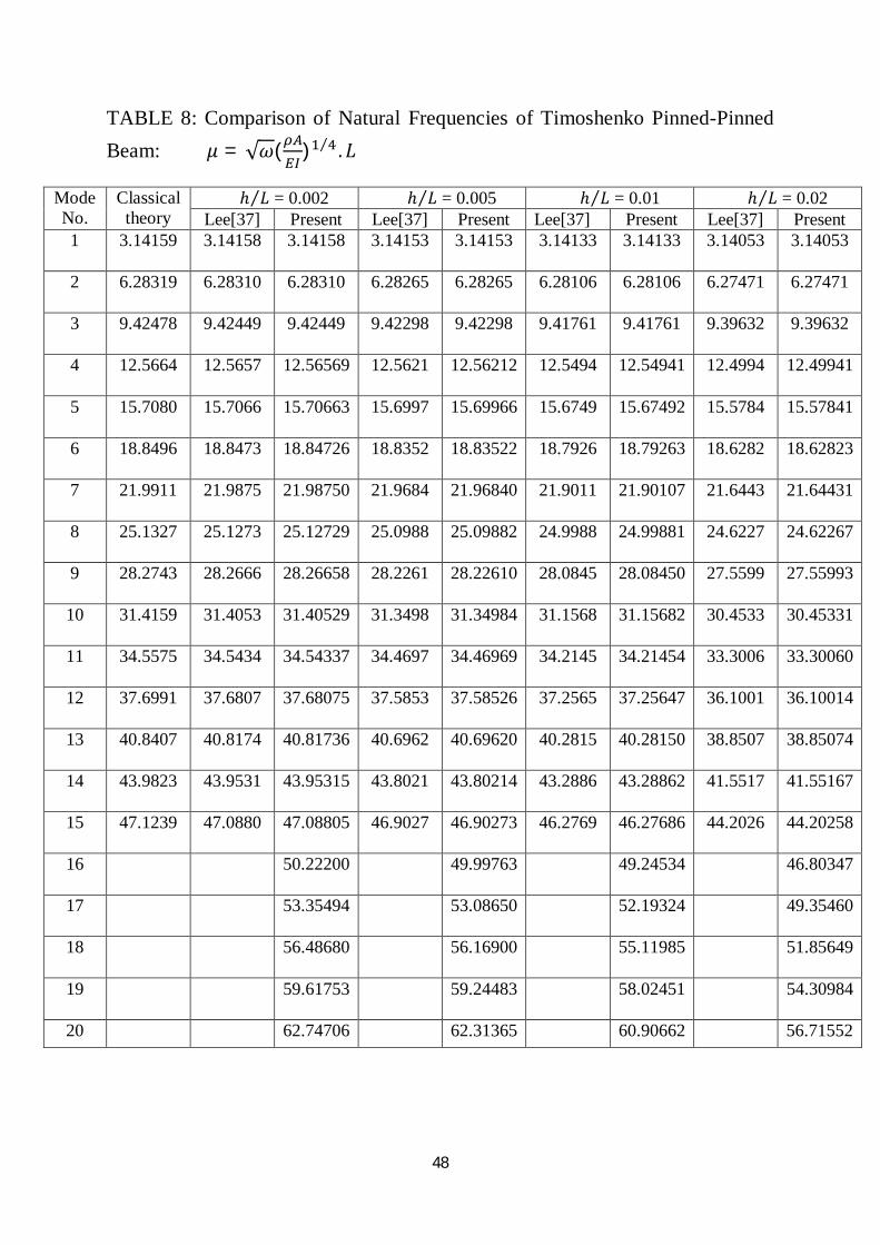
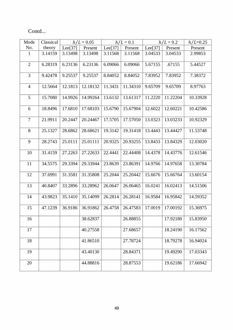
TABLE 8: Comparison of Natural Frequencies of Timoshenko Pinned-Pinned Beam: 휇 = √휔( ) ⁄ . 퐿
Mode No.
Classical theory
ℎ 퐿⁄ = 0.002 ℎ 퐿⁄ = 0.005 ℎ 퐿⁄ = 0.01 ℎ 퐿⁄ = 0.02 Lee[37] Present Lee[37] Present Lee[37] Present Lee[37] Present
1 3.14159 3.14158 3.14158 3.14153 3.14153 3.14133 3.14133 3.14053 3.14053
2 6.28319 6.28310 6.28310 6.28265 6.28265 6.28106 6.28106 6.27471 6.27471
3 9.42478 9.42449 9.42449 9.42298 9.42298 9.41761 9.41761 9.39632 9.39632
4 12.5664 12.5657 12.56569 12.5621 12.56212 12.5494 12.54941 12.4994 12.49941
5 15.7080 15.7066 15.70663 15.6997 15.69966 15.6749 15.67492 15.5784 15.57841
6 18.8496 18.8473 18.84726 18.8352 18.83522 18.7926 18.79263 18.6282 18.62823
7 21.9911 21.9875 21.98750 21.9684 21.96840 21.9011 21.90107 21.6443 21.64431
8 25.1327 25.1273 25.12729 25.0988 25.09882 24.9988 24.99881 24.6227 24.62267
9 28.2743 28.2666 28.26658 28.2261 28.22610 28.0845 28.08450 27.5599 27.55993
10 31.4159 31.4053 31.40529 31.3498 31.34984 31.1568 31.15682 30.4533 30.45331
11 34.5575 34.5434 34.54337 34.4697 34.46969 34.2145 34.21454 33.3006 33.30060
12 37.6991 37.6807 37.68075 37.5853 37.58526 37.2565 37.25647 36.1001 36.10014
13 40.8407 40.8174 40.81736 40.6962 40.69620 40.2815 40.28150 38.8507 38.85074
14 43.9823 43.9531 43.95315 43.8021 43.80214 43.2886 43.28862 41.5517 41.55167
15 47.1239 47.0880 47.08805 46.9027 46.90273 46.2769 46.27686 44.2026 44.20258
16 50.22200 49.99763 49.24534 46.80347
17 53.35494 53.08650 52.19324 49.35460
18 56.48680 56.16900 55.11985 51.85649
19 59.61753 59.24483 58.02451 54.30984
20 62.74706 62.31365 60.90662 56.71552
49
Contd...
Mode No.
Classical theory
ℎ 퐿⁄ = 0.05 ℎ 퐿⁄ = 0.1 ℎ 퐿⁄ = 0.2 ℎ 퐿⁄ =0.25 Lee[37] Present Lee[37] Present Lee[37] Present Present
1 3.14159 3.13498 3.13498 3.11568 3.11568 3.04533 3.04533 2.99853
2 6.28319 6.23136 6.23136 6.09066 6.09066 5.67155 .67155 5.44527
3 9.42478 9.25537 9.25537 8.84052 8.84052 7.83952 7.83952 7.38372
4 12.5664 12.1813 12.18132 11.3431 11.34310 9.65709 9.65709 8.97763
5 15.7080 14.9926 14.99264 13.6132 13.61317 11.2220 11.22204 10.33928
6 18.8496 17.6810 17.68103 15.6790 15.67904 12.6022 12.60221 10.42586
7 21.9911 20.2447 20.24467 17.5705 17.57050 13.0323 13.03233 10.92329
8 25.1327 28.6862 28.68621 19.3142 19.31418 13.4443 13.44427 11.53748
9 28.2743 25.0111 25.01111 20.9325 20.93255 13.8433 13.84329 12.03020
10 31.4159 27.2263 27.22633 22.4441 22.44408 14.4378 14.43776 12.61546
11 34.5575 29.3394 29.33944 23.8639 23.86391 14.9766 14.97658 13.30784
12 37.6991 31.3581 31.35808 25.2044 25.20442 15.6676 15.66764 13.60154
13 40.8407 33.2896 33.28962 26.0647 26.06465 16.0241 16.02413 14.51506
14 43.9823 35.1410 35.14099 26.2814 26.28141 16.9584 16.95842 14.59352
15 47.1239 36.9186 36.91862 26.4758 26.47583 17.0019 17.00192 15.36975
16 38.62837 26.88855 17.92180 15.83950
17 40.27558 27.68657 18.24190 16.17562
18 41.86510 27.78724 18.79278 16.94024
19 43.40130 28.84371 19.49290 17.03343
20 44.88816 28.87553 19.62186 17.66942
50
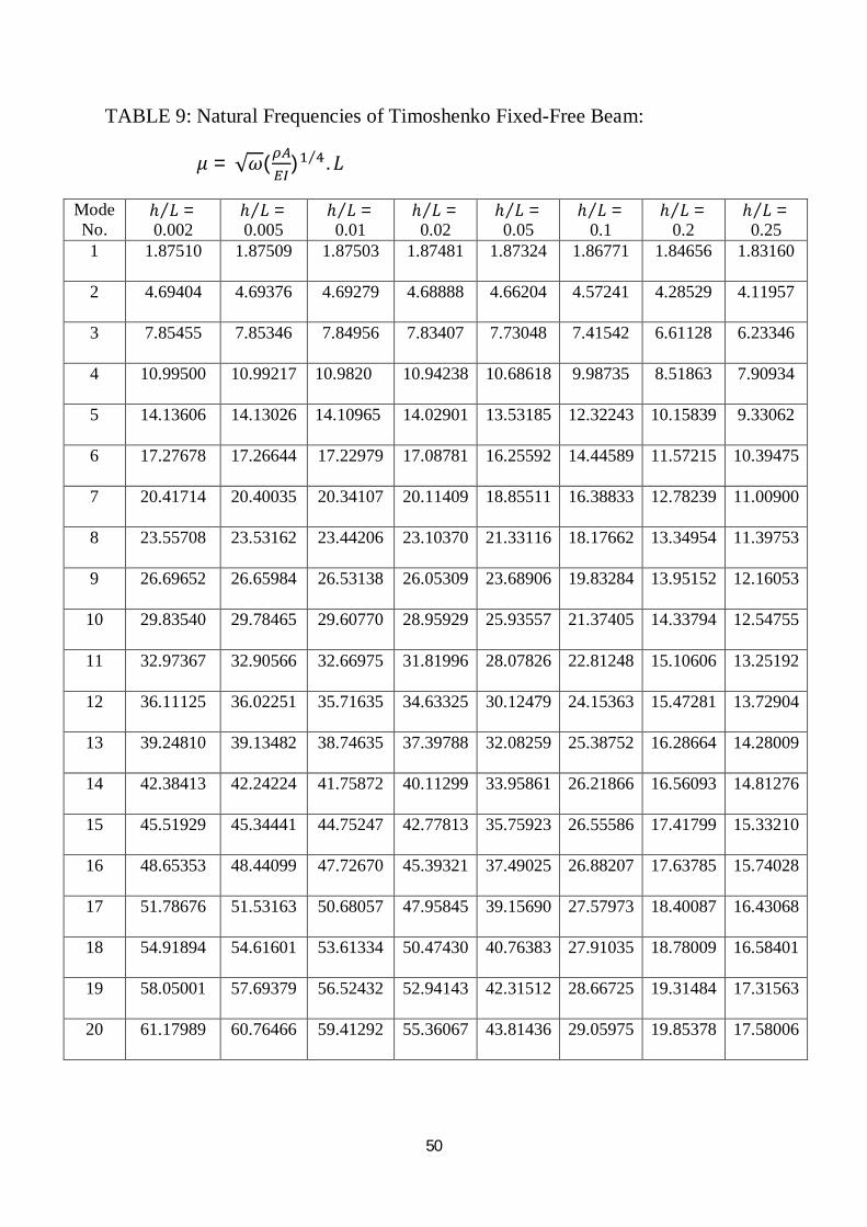
TABLE 9: Natural Frequencies of Timoshenko Fixed-Free Beam:
휇 = √휔( ) ⁄ . 퐿
Mode No.
ℎ 퐿 =⁄ 0.002
ℎ 퐿 =⁄ 0.005
ℎ 퐿 =⁄ 0.01
ℎ 퐿 =⁄ 0.02
ℎ 퐿 =⁄ 0.05
ℎ 퐿 =⁄ 0.1
ℎ 퐿 =⁄ 0.2
ℎ 퐿 =⁄ 0.25
1 1.87510 1.87509 1.87503 1.87481 1.87324 1.86771 1.84656 1.83160
2 4.69404 4.69376 4.69279 4.68888 4.66204 4.57241 4.28529 4.11957
3 7.85455 7.85346 7.84956 7.83407 7.73048 7.41542 6.61128 6.23346
4 10.99500 10.99217 10.9820 10.94238 10.68618 9.98735 8.51863 7.90934
5 14.13606 14.13026 14.10965 14.02901 13.53185 12.32243 10.15839 9.33062
6 17.27678 17.26644 17.22979 17.08781 16.25592 14.44589 11.57215 10.39475
7 20.41714 20.40035 20.34107 20.11409 18.85511 16.38833 12.78239 11.00900
8 23.55708 23.53162 23.44206 23.10370 21.33116 18.17662 13.34954 11.39753
9 26.69652 26.65984 26.53138 26.05309 23.68906 19.83284 13.95152 12.16053
10 29.83540 29.78465 29.60770 28.95929 25.93557 21.37405 14.33794 12.54755
11 32.97367 32.90566 32.66975 31.81996 28.07826 22.81248 15.10606 13.25192
12 36.11125 36.02251 35.71635 34.63325 30.12479 24.15363 15.47281 13.72904
13 39.24810 39.13482 38.74635 37.39788 32.08259 25.38752 16.28664 14.28009
14 42.38413 42.24224 41.75872 40.11299 33.95861 26.21866 16.56093 14.81276
15 45.51929 45.34441 44.75247 42.77813 35.75923 26.55586 17.41799 15.33210
16 48.65353 48.44099 47.72670 45.39321 37.49025 26.88207 17.63785 15.74028
17 51.78676 51.53163 50.68057 47.95845 39.15690 27.57973 18.40087 16.43068
18 54.91894 54.61601 53.61334 50.47430 40.76383 27.91035 18.78009 16.58401
19 58.05001 57.69379 56.52432 52.94143 42.31512 28.66725 19.31484 17.31563
20 61.17989 60.76466 59.41292 55.36067 43.81436 29.05975 19.85378 17.58006
51
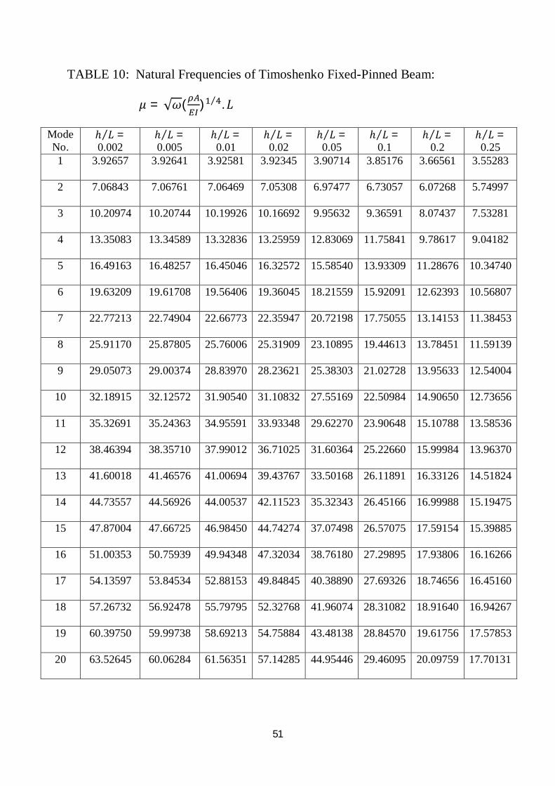
TABLE 10: Natural Frequencies of Timoshenko Fixed-Pinned Beam:
휇 = √휔( ) ⁄ . 퐿
Mode No.
ℎ 퐿 =⁄ 0.002
ℎ 퐿 =⁄ 0.005
ℎ 퐿 =⁄ 0.01
ℎ 퐿 =⁄ 0.02
ℎ 퐿 =⁄ 0.05
ℎ 퐿 =⁄ 0.1
ℎ 퐿 =⁄ 0.2
ℎ 퐿 =⁄ 0.25
1 3.92657 3.92641 3.92581 3.92345 3.90714 3.85176 3.66561 3.55283
2 7.06843 7.06761 7.06469 7.05308 6.97477 6.73057 6.07268 5.74997
3 10.20974 10.20744 10.19926 10.16692 9.95632 9.36591 8.07437 7.53281
4 13.35083 13.34589 13.32836 13.25959 12.83069 11.75841 9.78617 9.04182
5 16.49163 16.48257 16.45046 16.32572 15.58540 13.93309 11.28676 10.34740
6 19.63209 19.61708 19.56406 19.36045 18.21559 15.92091 12.62393 10.56807
7 22.77213 22.74904 22.66773 22.35947 20.72198 17.75055 13.14153 11.38453
8 25.91170 25.87805 25.76006 25.31909 23.10895 19.44613 13.78451 11.59139
9 29.05073 29.00374 28.83970 28.23621 25.38303 21.02728 13.95633 12.54004
10 32.18915 32.12572 31.90540 31.10832 27.55169 22.50984 14.90650 12.73656
11 35.32691 35.24363 34.95591 33.93348 29.62270 23.90648 15.10788 13.58536
12 38.46394 38.35710 37.99012 36.71025 31.60364 25.22660 15.99984 13.96370
13 41.60018 41.46576 41.00694 39.43767 33.50168 26.11891 16.33126 14.51824
14 44.73557 44.56926 44.00537 42.11523 35.32343 26.45166 16.99988 15.19475
15 47.87004 47.66725 46.98450 44.74274 37.07498 26.57075 17.59154 15.39885
16 51.00353 50.75939 49.94348 47.32034 38.76180 27.29895 17.93806 16.16266
17 54.13597 53.84534 52.88153 49.84845 40.38890 27.69326 18.74656 16.45160
18 57.26732 56.92478 55.79795 52.32768 41.96074 28.31082 18.91640 16.94267
19 60.39750 59.99738 58.69213 54.75884 43.48138 28.84570 19.61756 17.57853
20 63.52645 60.06284 61.56351 57.14285 44.95446 29.46095 20.09759 17.70131
52
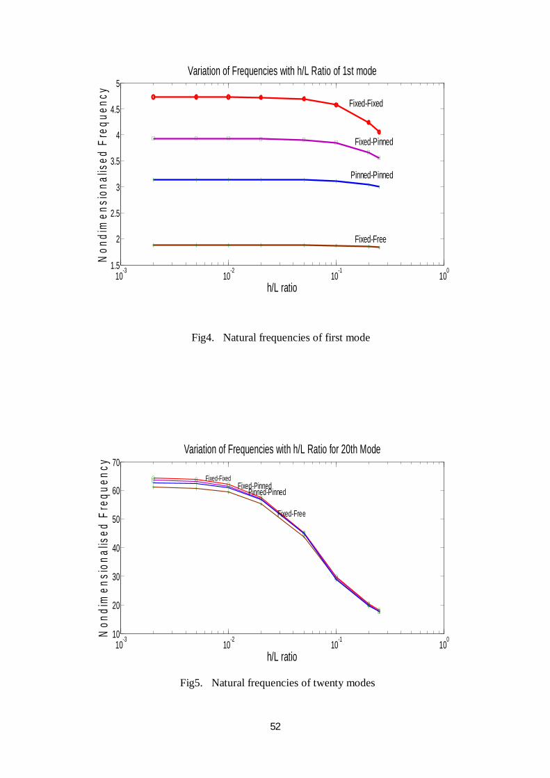
Fig4. Natural frequencies of first mode
Fig5. Natural frequencies of twenty modes
10-3
10-2
10-1
1001.5
2
2.5
3
3.5
4
4.5
5
Fixed-Fixed
Fixed-Free
Fixed-Pinned
Pinned-Pinned
h/L ratio
Non
dim
ensi
onal
ised
Fre
quen
cy
Variation of Frequencies with h/L Ratio of 1st mode
10-3 10-2 10-1 10010
20
30
40
50
60
70Fixed-Fixed
Fixed-Free
Fixed-PinnedPinned-Pinned
h/L ratio
Non
dim
ensi
onal
ised
Fre
quen
cy
Variation of Frequencies with h/L Ratio for 20th Mode
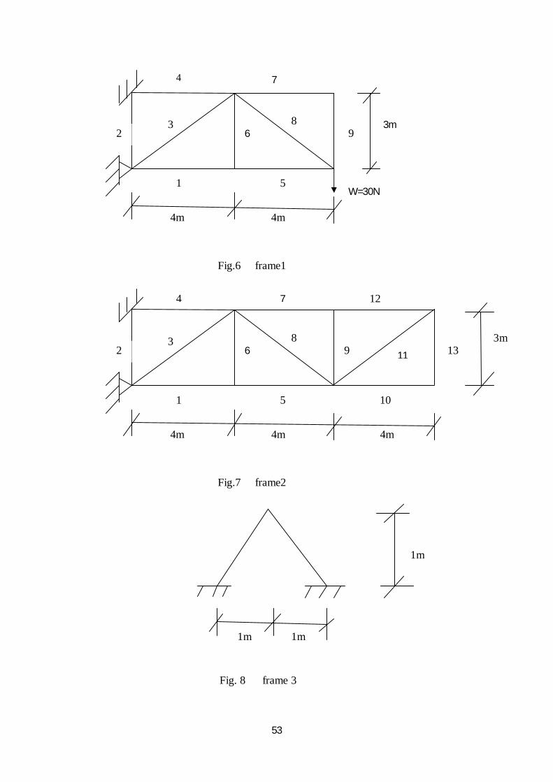
53
4m 4m
Fig.6 frame1
4m 4m 4m
Fig.7 frame2
Fig. 8 frame 3
1
2 3
4
5
6
7
8 9
3m
1
2 3
5
6 8
9
4 7
10
11
12
13 3m
W=30N
1m 1m
1m
54
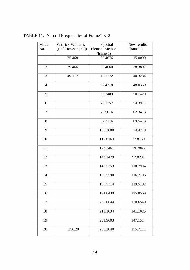
TABLE 11: Natural Frequencies of Frame1 & 2
Mode No.
Wittrick-Williams (Ref. Howson [32])
Spectral Element Method (frame 1)
New results (frame 2)
1 25.468 25.4676
15.0090
2 39.466 39.4660
38.3807
3 49.117 49.1172
40.3284
4 52.4718
48.0350
5 66.7489
50.1420
6 75.1757
54.3971
7 78.5016
62.3413
8 92.3116
69.5413
9 106.2880
74.4279
10 119.6163
77.8150
11 123.2461
79.7845
12 143.1479
97.8281
13 148.5353
110.7994
14 156.5590
116.7796
15 190.5314
119.5192
16 194.8439
125.8569
17 206.0644
130.6540
18 211.1034
141.1025
19 233.9603
147.1514
20 256.20 256.2040
155.7111
55
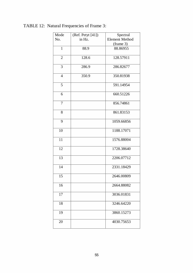
TABLE 12: Natural Frequencies of Frame 3:
Mode No.
(Ref. Petyt [41]) in Hz.
Spectral Element Method (frame 3)
1 88.9
88.86955
2 128.6
128.57911
3 286.9 286.82677
4 350.9 350.81938
5 591.14954
6 660.51226
7 856.74861
8 861.83153
9 1059.66856
10 1188.17071
11 1576.88004
12 1728.38640
13 2206.07712
14 2331.18429
15 2646.00809
16 2664.88082
17 3036.01831
18 3246.64220
19 3860.15273
20 4030.75653
56
CHAPTER 5
Conclusion
57
1. The Spectral Element Method (SEM) has the advantages of Spectral Analysis Method
(SAM), Dynamic Stiffness Method (DSM) and Finite Element Method (FEM).
2. The Spectral Element Method is efficient to compute both the lower and higher
modes natural frequencies even with a maximum number of two elements.
3. The natural frequencies of rods and beams up to the twenty numbers of modes have
been presented by using two number of spectral element.
4. The natural frequencies of frames have been presented up to the twentieth mode by
considering each member of the frame as a single element.
5. The finite element method couldn’t converge to the exact frequencies even with 200
numbers of finite elements. In some cases with these many numbers of elements it
couldn’t converge even further first mode frequency.
6. The natural frequencies of rods, beams and frames for various boundary conditions
are presented for the modes up to twenty where many higher modes results are not
available in the literature.
58
SCOPE OF FUTURE WORK
Through this project work some studies for the frequencies of rods, beams and frames are
attempted but still many areas are left which require further investigation. The possible
extensions to the present study are as given below:
1. The Spectral Element Method may be used for buckling analysis of structures.
2. The Spectral Element Method may be extended for the dynamic study of composite
beam, composite plates and structures of Functionally Graded materials.
3. The Spectral Element Method may be extended for response analysis of structures.
4. The Spectral Element Method may be used for dynamics of axially moving structures.
5. The Spectral Element Method may be applied to smart structures.
59
References
60
[1] Abramovich, H. Shear deformation and rotatory inertia effects of vibrating composites
beams. Composite structure, 20, 165-173, 1992.
[2] Abramovich, H. and Livshits, A. Free vibration of non-symmetric cross-ply laminated
composite beams. Journal of Sound and Vibration, 176, 597-612. 1994.
[3] Akesson, B. PFVIBAT- a computer programme for plane frame vibration analysis by an
exact method. International Journal for Numerical Methods in Engineering.10, 1221-1231,
1976.
[4] Armstrong, I. D. The natural frequencies of grillages.International Journal of Mechanical
Science, Pergamon Press, 10, 43-55, 1968.
[5] Banerjee, J. R. Free vibration of axially loaded composite Timoshenko beams using the
dynamic stiffness matrix method. Computers and Structures,69, 197-208. 1998.
[6] Banerjee, J. R. Free vibration analysis of a twisted beam using the dynamic stiffness
method. International Journal of Solids and Structures, 38, 6703-6722. 2001.
[7] Banerjee, J. R. Free vibration of centrifugally stiffened uniform and tapered beams using
the dynamic stiffness method. Journal of Sound and Vibration, 233, 857-875, 2000.
[8] Banerjee, J. R. Development of an exact dynamic stiffness matrix for free vibration
analysis of a twisted Timoshenko beam. Journal of Sound and Vibration, 270, 379-401. 2004.
[9] Banerjee, J. R. Dynamic stiffness formulation for structural elements: A general approach.
Computers and Structures, 63(1), 101-103, 1997.
[10] Banerjee, J. R, Guo, S.and Howson, W. P. Exact dynamic stiffness matrix of a bending-
torsion coupled beam including warping. Computers & structures.59, 613-621, 1996.
61
[11] Banerjee, J. R and Fisher, S. A. Coupled bending torsional dynamic stiffness matrix for
axially loaded beam element. International Journal numer.Meth.Engng, 33, 739-751, 1992.
[12] Banerjee, J. R and Williams, F.W. Clamped-Clamped natural frequencies of a bending-
torsion coupled beam. Journal of Sound and Vibration.176, 301-306, 1994.
[13] Banerjee, J. R. Coupled bending-torsional dynamic stiffness matrix for beam elements.
International Journal for numerical Methods in Engineering, 28, 1283-1298, 1989.
[14] Banerjee, J. R and Williams, F.W. Vibration of composite beams-an exact method using
symbolic computation. Journal of Aircraft, 32, 636-642. 1995.
[15] Banerjee, J. R and Williams, F.W. Exact dynamic stiffness matrix for composite
Timoshenko beams with applications.Journal of Sound and Vibration, 194, 573-585. 1996.
[16] Banerjee, J. R and Williams, F.W. An exact dynamic stiffness matrix for coupled-
extensional-torsional vibration of structural members.Computers and Structures, 50, 161-166,
1994.
[17] ] Banerjee, J. R and Williams, F.W. Coupled bending torsional dynamic stiffness matrix
for Timoshenko beam elements.Computers and Structures, 42,301-310, 1992.
[18] Banerjee, J. R and Williams, F.W. Exact Bernouli-Euler Dynamic Stiffness Matrix for a
ranged of Tapered beams. International Journal of numerical Methods in Engineering, 21,
2289-2302, 1985.
[19] Banerjee, J. R and Williams, F.W. Coupled bending torsional dynamic stiffness matrix
of an axially loaded Timoshenko beam element. International Journal of solids structure, 31,
749-762, 1994.
62
[20] Beskos, D. E. and Narayanan, G. V. Use of dynamic influence coefficients in forced
vibration problems with the aid of fast Fourier transform. Computer & structures.9, 145-150,
1978.
[21] Capron, M. D. And Williams, F. W. Exact dynamic stiffness for an axially loaded
uniform Timoshenko member embedded in an elastic medium. Journal of Sound and
Vibration, 124, 453-466, 1988.
[22] Chakraborty, A. And Gopalkrishinan, S. A spectrally formulated finite element for
wave propagation analysis in functionally graded beams. International Journal of solids and
structures,40 (10), 2421-2448, 2003.
[23] Chandrasekhar, K., Krishnamurthy, K. and Roy, S. Free vibration of composite beams
including rotatory inertia and shear deformation. Composites Structures, 14, 269-279, 1990.
[24] Cheng, F. Y. Vibration of Timoshenko beams and frameworks. Journal of the structural
division, 96, 551-571. 1970.
[25] Cheng, F. Y. and Tseng, W. H. Dynamic matrix of Timoshenko beam column. Journal
of the structural division.99, 527-549. 1973.
[26] Cho, J. and Lee, U. An FFT-based spectral analysis method for linear discrete dynamic
systems with non-proportional damping, Shock and Vibration, 13 (6), 595-606, 2006.
[27] Doyle, J. F. A Spectrally formulated finite elements for longitudinal wave propagation.
International Journal of Analytical and Experimental Modal Analysis, 3, 1-5, 1988.
[28] Doyle, J. F. Wave propagation in structures: Spectral Analysis Using Fast Discrete
Fourier Transforms, 2ndedn,Springer-Verlag, New York. 1997.
63
[29] Eisenberger, M. Abramovich, H. and Shulepov, O. Dynamic stiffness analysis of
laminated beams using a first order shear deformation theory. Composites Structures, 31,
265-271, 1995.
[30] Friberg, P. O. Coupled vibration of beams-an exact dynamic element stiffness matrix.
International Journal of numer. Meth.Engng, 19, 479-493, 1983.
[31] Gopalakrishna, S. And Doyle, J. F. Wave propagation in connected waveguides of
varying cross-section. Journal of Sound and Vibration, 175 (3), 347-363, 1994.
[32] Howson, W. P. A compact method for computing the eigenvalues and eigenvectors of
plane frames.
[33] Howson, W.P. and Williams, F. W. Natural frequencies of frames with axially loaded
Timoshenko members. Journal of Sound and vibration, 26, 503-515. 1973.
[34] Howson, W.P. and Zare, A. Exact dynamic stiffness matrix for flexural vibration of the
three-layered sandwich beams. I. Forward calculation. Journal of Sound and Vibration, 282,
(3-5), 753-767, 2005.
[35] Kolousek, V. Anwendung des gesetzes der virtuellenverschiebungen und des
reziprozitatssatzes in der stabwerksdynamic. IngenieurArchiv, 12, 363-370.1941.
[36] Lunden, R. and Akesson, B. Damped second-order Rayleigh-Timoshenko beam
vibration in space- an exact complex dynamic member stiffness matrix. International Journal
for Numerical Methods in Engineering.19, 431-449, 1983.
[37] Lee, J. and Schultz, W. W. Eigenvalue analysis of Timoshenko beams and
axisymmetric Mindlin plates by the pseudospectral method. Journal of Sound and Vibration,
269, 609-621, 2004.
64
[38] Lee, U. Spectral Element Method in Structural Dynamics. 2009.
[39] Narayanam, G.V. and Beskos,D.E. Use the dynamic influence coefficients in forced
vibration problems with the aid of fast fourier transform. Computer & structures, 9 (2),145-
150,1978.
[40] Przemieniecki, J.S. Theory of Matrix Structural Analysis, McGrow-Hill Inc, New
York.1968.
[41] Petyt, M. Introduction to Finite Element Vibration Analysis . Cambridge University
Press, 1990.
[42] Rizzi, S. A. And Doyle, J. F.A spectral element approach to wave motion in layered
solids, Journal of Vibration and Acoustics.114 (4), 569-577, 1992.
[43] Rosen, A. Structural and dynamics behaviour of pretwisted rods and beams. Applied
Mechanics Reviews, 44, 483-515, 1991.
[44] Teh, K. K. and Huang, C. C., The effects of fibre orientation on free vibration of
composite beams. Journal of Sound and Vibration, 69, 327-337, 1980.
[45] Teoh, S. L. and Huang, C. C., The vibration of beams of fibre reinforced
material.Journal of Sound and Vibration, 51, 467-473,1977.
[46] Wang, T. M. and Kinsman, T. A. Vibration of frame structures according to the
Timoshenko theory. Journal of Sound and Vibration, 14, 215-227, 1971.
[47] Wittrick, W. H. and Williams F. W. A general algorithm for computing natural
frequencies of elastic sttructures.Quarterly Journal of Mechanics and Applied Mathematics,
24, 263-284,1971.
65
[48] Wittrick, W. H. and Williams, F. W. Exact buckling and frequency calculation surveyed.
Journal Structures. Engng ASCE. 109, 169-187, 1983.
[49] Wittrick, W. H. and Williams, F. W. An Automatic computational procedure for
calculating natural frequencies of skeletal Structures.Intenational Journal. Mech.
Sci.Pergamon Press. 12, 781-791, 1970.
[50] Yang, Bingen. Stress Strain and Structural Dynamics. Elsevier Academic Press, 2005.