Embed Size (px)
Citation preview
8/11/2019 Fundamentals of Acoustically Coupled Combustions
http://slidepdf.com/reader/full/fundamentals-of-acoustically-coupled-combustions 1/120
6-1
DYNAMICS OF COMBUSTION SYSTEMS:
FUNDAMENTALS, ACOUSTICS, AND
CONTROL
A Short Course of Lectures
VI. FUNDAMENTALS OF ACOUSTICS
F.E.C. CULICK
California Institute of Technology
September 2001
2001 by F.EC. Culick
All Rights Reserved
8/11/2019 Fundamentals of Acoustically Coupled Combustions
http://slidepdf.com/reader/full/fundamentals-of-acoustically-coupled-combustions 2/1206-2
FUNDAMENTALS OF ACOUSTICS
According to the experiences cited and the reasoning given in Section I,
combustion instabilities may be regarded as unsteady motions closely
approximated as classical acoustical motions with perturbations due to
combustion processes.
The framework for analyzing and interpreting combustion instabilities has
from the beginning been constructed with strong guidance by the principles
of classical acoustics. Moreover, as a general strategy in studying
combustion instabilities it is useful to concentrate first on gas dynamics as a
means of interpreting observed behavior. Deficiencies then require appeal
to other processes, notably those associated with combustion.
It is therefore essential to have a sound understanding of the behavior of
small amplitude motions in a compressible medium with no combustion
processes.
This section covers the parts of classical acoustics which in some degree
influence the subject of combustion instabilities.
The material included here covers only the essentials of small amplitude
motions in chambers and tubes, with no combustion and average flow.
Inhomogeneities in the medium are not included; interesting problems
therefore arise only if boundaries and sources are explicitly present.
In the narrow form considered here, acoustics comprises problems of wave
motion interior to regions partially or totally enclosed by prescribed
boundaries.
References: Morse, P.M., Vibration and Sound
Morse, P.M. and Ingard, K.U., Theoretical Acoustics
Landau, L.D. and Lifschitz, E.M., Fluid Mechanics
Temkin, R., Elements of Acoustics
8/11/2019 Fundamentals of Acoustically Coupled Combustions
http://slidepdf.com/reader/full/fundamentals-of-acoustically-coupled-combustions 3/1206-3
6.1 LINEARIZATION OF THE EQUATIONS OF
MOTION; THE WAVE EQUATION AND THE
VELOCITY POTENTIAL
The influences of viscous effects are normally small within the
volume; they are examined later. Here the discussion is based
on the inviscid equations of motion for a homogeneous medium
free of inhomogeneities and sources:
Conservation of Mass
Conservation of Momentum
Conservation of Energy
Equation of State
0=⋅∇+∂
∂ )u(
t
r ρ
ρ
0=∇+∇⋅+∂
∂ puu
t
u rrr ρ ρ
02
1
2
1 22 =⋅∇+
+∇⋅+
+
∂
∂ )u(pueuue
t
rr ρ ρ
RT p ρ =
Remove the kinetic energy from the energy equation by
subtracting
0or 0 =⋅∇+=⋅∇+∇⋅+∂
∂u p
Dt
De u peu
t
e rrr ρ ρ ρ
( ) :equationmomentum⋅ur
6.1.1 Conservation Equations of Motion
8/11/2019 Fundamentals of Acoustically Coupled Combustions
http://slidepdf.com/reader/full/fundamentals-of-acoustically-coupled-combustions 4/1206-4
The equation for the entropy of a fluid element is:
Substitution of the mass and energy equations gives:
Because all irreversible processes have been ignored, the motions
within the volume are necessarily isentropic.
∇⋅+∂
∂=−= u
t Dt
D
Dt
D
Dt
De
Dt
Ds r
p ;
ρ
ρ ρ ρ
0)( =⋅∇+⋅∇−= u p
u p Dt
Ds rr ρ
ρ ρ
Changes of density are given by:
will turn out to be the speed of propagation of small disturbances —
the “speed of sound”
dpadp p
dp p
ds s
d s s p
2=
∂
∂=
∂
∂+
∂
∂=
ρ ρ ρ ρ
Where we assume an isentropic process and
s
dpa
∂= ρ 2
6.1 LINEARIZATION OF THE EQUATIONS OF
MOTION; THE WAVE EQUATION AND THE
VELOCITY POTENTIAL
6.1.1 Conservation Equations of Motion (cont’d)
8/11/2019 Fundamentals of Acoustically Coupled Combustions
http://slidepdf.com/reader/full/fundamentals-of-acoustically-coupled-combustions 5/1206-5
The continuity equation can be written now for the pressure:
For more general applications it is useful to obtain this equation for
the pressure by adding the mass and energy equations with de =
C vdT and using the equation of state:
)( ∗=∇⋅+⋅∇+∂
∂ 02 puua
t
p rr ρ
( )
( ) (2) 0
(1) 0
=∇⋅+⋅∇+∂
∂
=∇⋅+⋅∇+∂
∂
T uuC
p
t
T
T uut
T
v
ρ ρ
ρ ρ ρ
rr
rr
( ) ( )
01
0
=∇⋅+⋅∇
++
∂
∂
=∇⋅+⋅∇
++
∂
∂
puu pC
R
t
p
T uuC
pT T
t
v
v
rr
rr ρ ρ ρ
But R = C p – C v, so R/C v = γ − 1 and equation (∗) is recovered
because γ p = ρa2 for the conditions assumed here,
ρ
γ pa =2
Add (1) and (2):
6.1 LINEARIZATION OF THE EQUATIONS OF
MOTION; THE WAVE EQUATION AND THE
VELOCITY POTENTIAL
6.1.1 Conservation Equations of Motion (cont’d)
8/11/2019 Fundamentals of Acoustically Coupled Combustions
http://slidepdf.com/reader/full/fundamentals-of-acoustically-coupled-combustions 6/1206-6
Note also the relation for the internal energy of a perfect gas,
because e = e(T), is a function of temperature only for a
perfect gas.
and the momentum equation can be written:
dT C dT T
edv
v
ede v
vT
=
∂
∂+
∂
∂=
For isentropic processes of a perfect gas,
00
γ
ρ
ρ
= p p
)( ∗∗=∇
+∇⋅+
∂
∂ 0
11/
0
0
p p
puu
t
u γ
ρ
rrr
Wave Equation for the Pressure
Differentiate (∗) with respect to time and substitute (∗∗) for
with a2 = γ p/ρ:t / u ∂∂r
( ) ( ) put
ut
puu p
p/p
p
p
pa
t
p∇⋅
∂
∂−⋅∇
∂
∂−∇⋅⋅∇=
∇⋅∇
−
∂
∂ rrrrγ γ
γ 1/00
202
2
)(
6.1 LINEARIZATION OF THE EQUATIONS OF
MOTION; THE WAVE EQUATION AND THE
VELOCITY POTENTIAL
6.1.1 Conservation Equations of Motion (cont’d)
8/11/2019 Fundamentals of Acoustically Coupled Combustions
http://slidepdf.com/reader/full/fundamentals-of-acoustically-coupled-combustions 7/1206-7
The boundary condition for this equation is set by taking the
component of (**) normal to the boundary:
6.1.2 Linearization of the Conservation Equations
Let ε be a small parameter characterizing the amplitude of
time-dependent motions superimposed upon a uniform state of
a gas at rest:
( )
∇⋅⋅+
∂
∂⋅
−=∇⋅ uun
t
un
p
p pn
rrr
ˆˆˆ 0
1/
0
ρ
γ
uu
p p p
′=
+=′+=
rrε
ερ ρ ρ
ε
'0
0
Nonlinear behavior arises in the present context mainly from
convection (i.e. etc.) and from the dependence
of the speed of sound on amplitude, .
pu ,uu ∇⋅∇⋅ rrr
6.1 LINEARIZATION OF THE EQUATIONS OF
MOTION; THE WAVE EQUATION AND THE
VELOCITY POTENTIAL
6.1.1 Conservation Equations of Motion (cont’d)
ρ γ γ / p RT a ==
8/11/2019 Fundamentals of Acoustically Coupled Combustions
http://slidepdf.com/reader/full/fundamentals-of-acoustically-coupled-combustions 8/1206-8
Substitute the assumed forms and expand to second order:
( ) ( )
( )
...11
...2
111
1
11
2
00
2
0
200
2
0
22001/
00
20
2
02
2
01/
01/
0
+
′∇−
′∇
′−+
′∇=
∇⋅∇
+
′
++
′−=
+=
p
p
p
p
p
pa p
p
pa p
p/p
p
p
pa
p
p
p
p
p'/p p/p
γ γ
γ ε
ε
γ
γ ε
γ ε
γ
γ γ
Substitute in the wave equation for p, collect terms according to
powers of ε and divide by ε :
The boundary condition becomes
Problems of linear acoustics are described by the equations obtained
in the limit ε = 0:
...11
)
2
00
2
0
200
022
02
2
+
′∇−
′∇
′−+
′∇⋅′
∂
∂−′⋅∇
∂
′∂−′∇⋅′⋅∇=′∇−
∂
′∂
p
p
p
p
p
pa p
pu( t
ut
p )uu( p pa
t
p
γ γ
γ
γ ε rrrr
( ) ...ˆˆ1
ˆˆ000
+
′∇⋅′⋅+⋅
∂
′∂′−⋅
∂
′∂−=′∇⋅ uunn
t
u
p
pn
t
u pn
rrrr
γ ερ ρ
nt
u pn
pat
p
ˆˆ
0
0
2202
2
⋅∂
′∂
−=′∇⋅
=′∇−∂
′∂
r
ρ
6.1 LINEARIZATION OF THE EQUATIONS OF
MOTION; THE WAVE EQUATION AND THE
VELOCITY POTENTIAL
6.1.2 Linearization of the Conservation Equations (cont’d)
8/11/2019 Fundamentals of Acoustically Coupled Combustions
http://slidepdf.com/reader/full/fundamentals-of-acoustically-coupled-combustions 9/1206-9
It is often convenient to introduce the scalar and vector potentials φand from which the velocity is found by differentiation: A
r
Aurr
×∇+∇−=′ φ
With this representation, the dilatation and curl (rotation) of the
velocity field are separated:
Auurrr
×∇×∇=′×∇−=⋅∇ ∇ ; 2φ
Here only the scalar potential is required for linear motions
because for small amplitudes, the pressure and momentum
equations become the equations for classical acoustics:
01
0
o
o
=′∇+∂
′∂
=′⋅∇+∂
′∂
pt u
ut
p
ρ
γρ
r
r
6.1 LINEARIZATION OF THE EQUATIONS OF
MOTION; THE WAVE EQUATION AND THE
VELOCITY POTENTIAL
6.1.3 Velocity Potential
8/11/2019 Fundamentals of Acoustically Coupled Combustions
http://slidepdf.com/reader/full/fundamentals-of-acoustically-coupled-combustions 10/1206-10
The pressure fluctuation is found from the relation:
022
2
2
=∇−∂
∂φ
φ oa
t
t p
∂
∂=′
φ ρ o
The second equation gives which means
Although it appears that non-zero may arise in
this limit, that is not the case in the present context.
,0=′×∇ ur
. A 0=×∇×∇ r
Ar
Combine the above two equations and substitute to fix the equation
for the velocity potential:
6.1 LINEARIZATION OF THE EQUATIONS OF
MOTION; THE WAVE EQUATION AND THE
VELOCITY POTENTIAL
6.1.3 Velocity Potential
8/11/2019 Fundamentals of Acoustically Coupled Combustions
http://slidepdf.com/reader/full/fundamentals-of-acoustically-coupled-combustions 11/1206-11
6.2 ELEMENTARY SOLUTIONS TO THE WAVE
EQUATION: PLANE, SPHERICAL, AND
CYLINDRICAL WAVES
6.2.1 Plane Waves
The basic property of linear problems is that the principle of
superposition applies. Solutions for more complicated problems can
often be constructed by superimposing elementary solutions.
Wave equation: 02
22
2
2
=∂
′−
∂
′∂ ∂ x
pa
t
po
can be factored 000 =′
∂
∂
−∂
∂
∂
∂
+∂
∂
p xat xat
and a general solution has the form
Pressure Waves t)a(x g t)a f(x p 00 −++=′
t):a(x g 0−
t):a f(x 0+ Wave to the left
Wave to the right
x: direction of propagation, so wave fronts or planes of
constant phase are normal to the x-axis.
8/11/2019 Fundamentals of Acoustically Coupled Combustions
http://slidepdf.com/reader/full/fundamentals-of-acoustically-coupled-combustions 12/1206-12
Density Waves
For a wave traveling to the right:
[ ]t)a(x g t)a(x f a p
p002
00
0 1' −++=
′=
γ
ρ ρ
Velocity Waves
Integrate [ ]t)a(x g t)a(x f p
a
t
p
p x
u002
0
0
0
1−′−+′=
∂
′∂−=
∂
′∂
γ γ
[ ]t)a(xgt)a(xf p
au 00
0
0 −−+−=′γ
00a pu ρ
′=′
For a wave traveling to the left:00a
pu
ρ
′−=′
6.2 ELEMENTARY SOLUTIONS TO THE WAVE
EQUATION: PLANE, SPHERICAL, AND
CYLINDRICAL WAVES
6.2.1 Plane Waves (cont’d)
8/11/2019 Fundamentals of Acoustically Coupled Combustions
http://slidepdf.com/reader/full/fundamentals-of-acoustically-coupled-combustions 13/1206-13
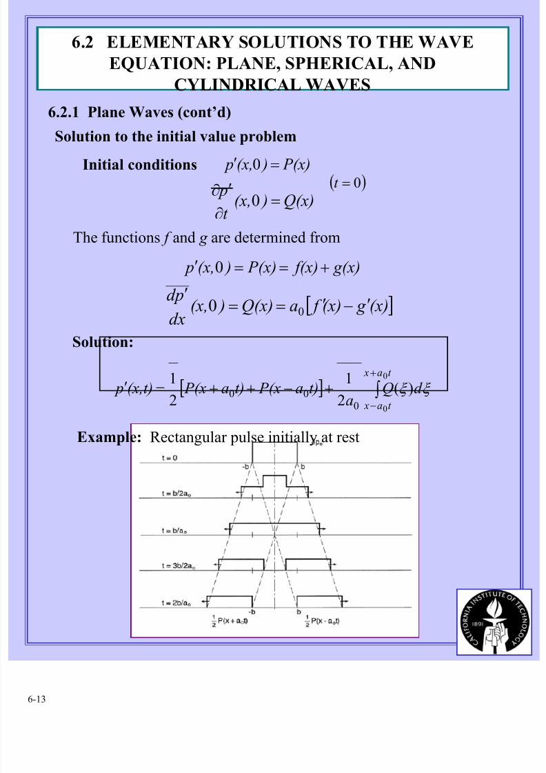
Solution to the initial value problem
Initial conditions P(x) )(x, p =′ 0
Q(x) )(x,t
p=
∂
′∂0
( )0=t
The functions f and g are determined from
[ ](x) g (x) f aQ(x) )(x,dx
pd ′−′==
′00
g(x) f(x) P(x) )(x, p +==′ 0
Solution:
[ ] ∫
+
−
+−++=′t a x
t a x
d Qa
t)a P(xt)a P(xt)(x, p0
0
)(2
1
2
1
000 ξ ξ
Example: Rectangular pulse initially at rest
6.2 ELEMENTARY SOLUTIONS TO THE WAVE
EQUATION: PLANE, SPHERICAL, AND
CYLINDRICAL WAVES
6.2.1 Plane Waves (cont’d)
8/11/2019 Fundamentals of Acoustically Coupled Combustions
http://slidepdf.com/reader/full/fundamentals-of-acoustically-coupled-combustions 14/1206-14
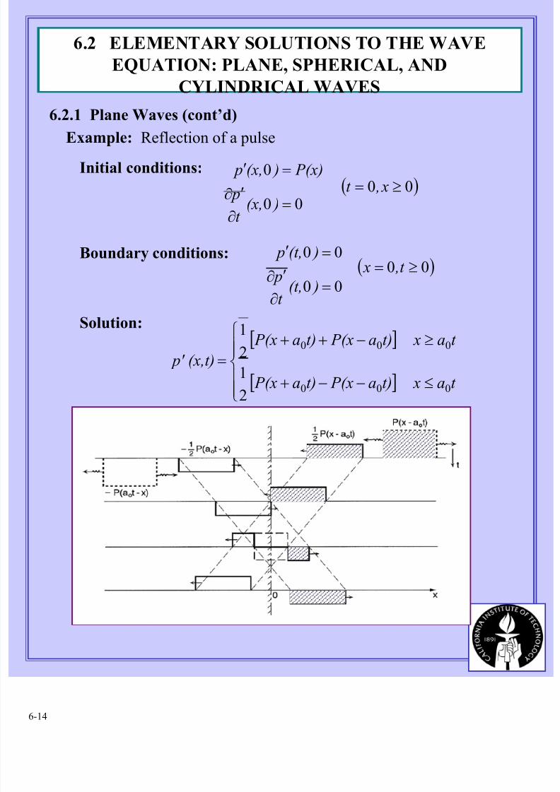
Example: Reflection of a pulse
Initial conditions:
00
0
=∂
′∂
=′
)(x,t
p
P(x) )(x, p( )00 ≥= x ,t
Boundary conditions:
00
00
=∂
′∂
=′
)(t,t
p
)(t, p
( )00 ≥= t , x
Solution:[ ]
[ ]
≤−−+
≥−++=
t a xt)a P(xt)a P(x
t a xt)a P(xt)a P(x
p' (x,t)
000
000
2
1
2
1
6.2 ELEMENTARY SOLUTIONS TO THE WAVE
EQUATION: PLANE, SPHERICAL, AND
CYLINDRICAL WAVES
6.2.1 Plane Waves (cont’d)
8/11/2019 Fundamentals of Acoustically Coupled Combustions
http://slidepdf.com/reader/full/fundamentals-of-acoustically-coupled-combustions 15/1206-15
Sinusoidal plane
waves)i(
(
0
)i(
)
0
00
00
t kxt)a x
ai
t kx
t a(x
a
i
Be Bet)a g(x
Ae Aet)a f(x
ω
ω
ω
ω
−±−±
+±
+±
==−
==+
frequency
λ
π ω
λ π π ω
2
22
0
0
==
==
ak
a f
wavenumber
6.2.2 Spherical Waves
Assume motions symmetric about a point: wave will propagate
inward or outward.
Wave equation: 01 2
2
20
2
2
=
∂
′∂
∂
∂−
∂
′∂
r
pr
r r a
t
p
Try a solution: )(1
t r,r
t)(r, p ψ =′
02
2202
2
=∂
∂−
∂
∂
r a
t
ψ ψ
and a solution for the pressure has the form:
Pressure Waves [ ]r)t G(ar)t F(ar
t)(r, p −++=′00
1
r):t F(a +0
r):t G(a −0
inward traveling wave
outward traveling wave
6.2 ELEMENTARY SOLUTIONS TO THE WAVE
EQUATION: PLANE, SPHERICAL, AND
CYLINDRICAL WAVES
6.2.1 Plane Waves (cont’d)
8/11/2019 Fundamentals of Acoustically Coupled Combustions
http://slidepdf.com/reader/full/fundamentals-of-acoustically-coupled-combustions 16/1206-16
An initial value problem for spherical waves
Initial conditions
Assume p′ finite at r = 0 :
To satisfy initial conditions:
Pressure Field:
W(r) )(r,t
p
V(r) )(r, p
=∂
′∂
=′
0
0)0( =t
[ ] [ ]t)G(at) F(ar
(r,t) pr
r 000
0
1+
=′
→→
)()( ξ ξ F G −=⇒
Hence [ ]r)t F(ar)t F(ar
(r,t) p −−+=′00
1
)(1
)()(
)()()(
0
ξ ξ ξ ξ
ξ ξ ξ
W a
F F
V F F
=−′−′
=−−
Assume medium initially at rest, W(r) = 0
>−−+++
<−−−++=
t)a(r t)at)V(r a(r r)t r)V(at (a
t)a(r r)t r)V(at (ar)t r)V(at (a
r p'(r,t)
00000
00000
2
1
6.2 ELEMENTARY SOLUTIONS TO THE WAVE
EQUATION: PLANE, SPHERICAL, AND
CYLINDRICAL WAVES
6.2.2 Spherical Waves (cont’d)
8/11/2019 Fundamentals of Acoustically Coupled Combustions
http://slidepdf.com/reader/full/fundamentals-of-acoustically-coupled-combustions 17/1206-17
Example
>
≤<=
0
00
0
0)(
r
r pV
ξ
ξ δ ξ
>−
>
≤−<
−−=
>−
<
≤−<
−−=
00
0
000
0
00
0
000
0
0
0
2
1
0
0
2
1
r t)a(r
t)a(r
r t)a(r p
t)a(r r
r r)t (a
t)a(r
r r)t (a p
r)t (ar
p'
δ
δ
6.2 ELEMENTARY SOLUTIONS TO THE WAVE
EQUATION: PLANE, SPHERICAL, AND
CYLINDRICAL WAVES
6.2.2 Spherical Waves (cont’d)
8/11/2019 Fundamentals of Acoustically Coupled Combustions
http://slidepdf.com/reader/full/fundamentals-of-acoustically-coupled-combustions 18/1206-18
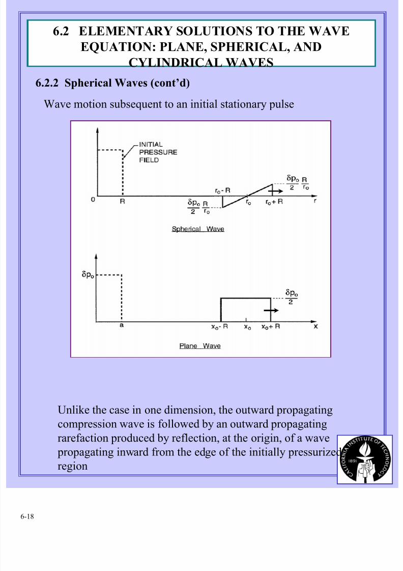
Wave motion subsequent to an initial stationary pulse
Unlike the case in one dimension, the outward propagating
compression wave is followed by an outward propagating
rarefaction produced by reflection, at the origin, of a wave
propagating inward from the edge of the initially pressurized
region
6.2 ELEMENTARY SOLUTIONS TO THE WAVE
EQUATION: PLANE, SPHERICAL, AND
CYLINDRICAL WAVES
6.2.2 Spherical Waves (cont’d)
8/11/2019 Fundamentals of Acoustically Coupled Combustions
http://slidepdf.com/reader/full/fundamentals-of-acoustically-coupled-combustions 19/1206-19
Velocity in an outward propagating spherical wave
+′+−=
∂
′∂−=
∂
′∂r)t (a F
r r)t F(a
r r
p
t
u002
00
1111
ρ ρ
∫∞−
′−′+−=′t
t r)d t F(ar
r)t F(ar a
(r,t)u 020
000
1111
ρ ρ
∫∞−
′′+′
=t
t d p
r a
pu(r,t)
000
1
ρ ρ
00a
pu(r,t)
ρ
′=
Spherical wave
Plane wave
In a spherical wave, the velocity disturbance may be zero where
the pressure disturbance is nonzero unless
∫ ∫∞−
∞
=′⇒=′′t
rdr pt d p0
00
for the wave to be confined to a finite radial extent
6.2 ELEMENTARY SOLUTIONS TO THE WAVE
EQUATION: PLANE, SPHERICAL, AND
CYLINDRICAL WAVES
6.2.2 Spherical Waves (cont’d)
8/11/2019 Fundamentals of Acoustically Coupled Combustions
http://slidepdf.com/reader/full/fundamentals-of-acoustically-coupled-combustions 20/1206-20
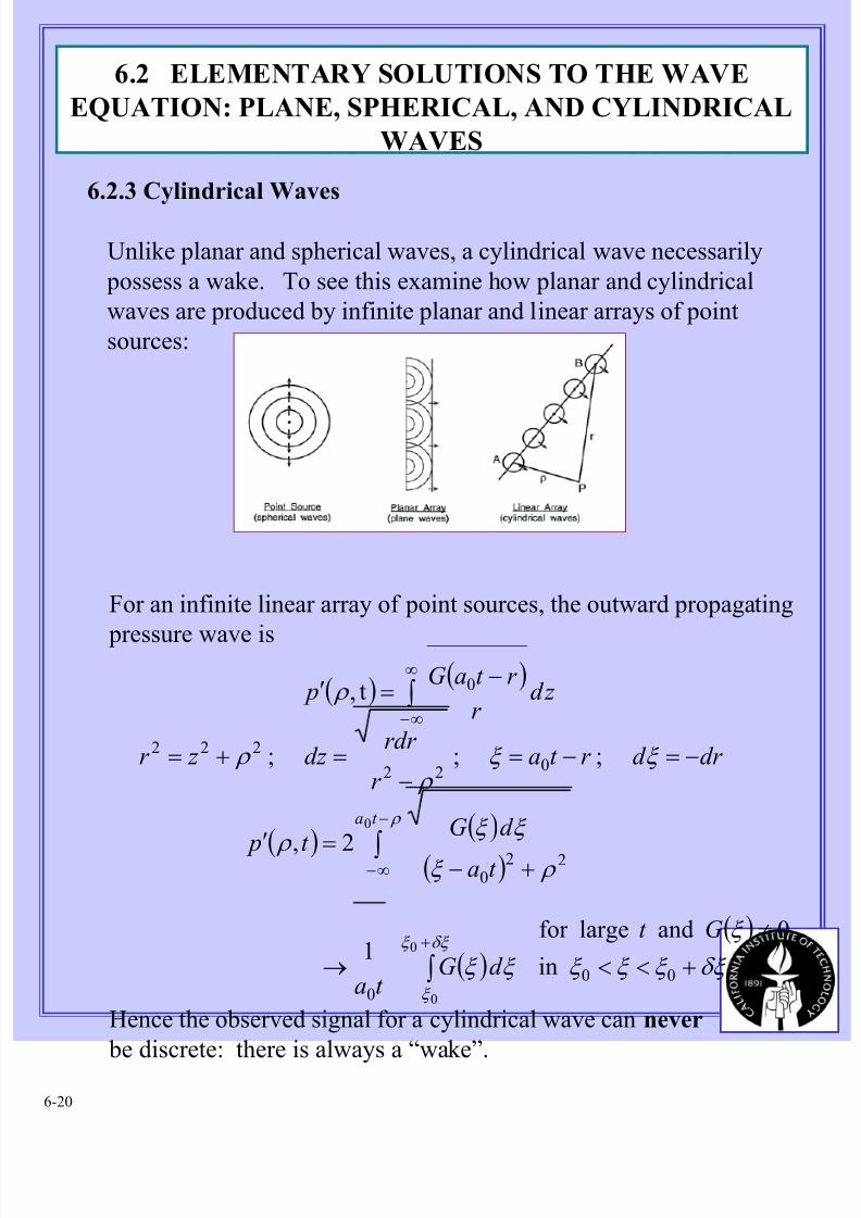
Unlike planar and spherical waves, a cylindrical wave necessarily
possess a wake. To see this examine how planar and cylindrical
waves are produced by infinite planar and linear arrays of point
sources:
For an infinite linear array of point sources, the outward propagating
pressure wave is
( ) ( )
z d r
r t aG p ∫
∞
∞−
−=′ 0t, ρ
dr d r t ar
rdr dz z r −=−=
−=+= ξ ξ
ρ ρ ;;; 022
222
Hence the observed signal for a cylindrical wave can never
be discrete: there is always a “wake”.
( ) ( )( )
( )1
2,
0
220
0
0
0
ξ ξ
ρ ξ ξ ξ ρ
δξ ξ
ξ
ρ
d Gt a
t ad Gt p
t a
∫
∫
+
−
∞−
→
+−=′
( )
δξ ξ ξ ξ
ξ
+<<
≠
00in
0 and largefor Gt
6.2 ELEMENTARY SOLUTIONS TO THE WAVE
EQUATION: PLANE, SPHERICAL, AND CYLINDRICAL
WAVES
6.2.3 Cylindrical Waves
8/11/2019 Fundamentals of Acoustically Coupled Combustions
http://slidepdf.com/reader/full/fundamentals-of-acoustically-coupled-combustions 21/1206-21
6.3 AN ESTIMATE OF THE INFLUENCE OF
HEAT CONDUCTION
Linearized
2
2c
x
T
C x
u
C
p
x
T u
t
T
vv ∂
∂=
∂
∂+
∂
∂+
∂
∂ λ ρ ρ
One-dimensional energy equation with heat conduction
2
2
00
0
x
T
C x
u
C
p
t
T
v
c
v ∂
′∂=
∂
′∂+
∂
′∂
ρ
λ
ρ
Eliminate by using the continuity equation
)( x
T
Cx
p
C
p
t
T2
2
v0
c
v20
0 ∗∂
′∂=∂
′∂−∂
′∂ ρ
λ
ρ
Linearized momentum equation
01
0
=∂
′∂+
∂
′∂
x
p
t
u
ρ
Motions are non-isentropic, and assume p = p(ρ,T )
dT T
pd
pdp
∂
∂+
∂
∂= ρ
ρ T
xu ∂′∂
Reference: Morse and Feshback (1952) Methods of Theoretical
Physics, Vol. 1, Chapter , Problem . .
8/11/2019 Fundamentals of Acoustically Coupled Combustions
http://slidepdf.com/reader/full/fundamentals-of-acoustically-coupled-combustions 22/1206-22
Combine with momentum and continuity equations:
)( ∗∗=∂
′∂
∂
∂−
∂
∂
∂
∂−
∂
∂ 0
''2
2
2
2
T2
2
00 x
T
T
p
x
p
t ρ
ρ
ρ
ρ
( ) ( )t kxit kxi eT T e ω ω ρ ρ −− =′= ˆ;ˆ'
( )
( ) 0ˆˆ
0ˆˆ
0
22
0
2
20
02
0
c
=
∂
∂−−
∂
∂⇒∗∗
=
−
+⇒∗
ρ ρ
ω
ρ ρ
ω ρ
λ ω
ρ T
vv
pk T
T
pk
C
piT k
C i
Assume sinusoidal travelling waves:
Substitute in (∗) and (∗∗):
Non-trivial solutions for and only if: ρ ˆ T
( )∗∗∗=
−
∂
∂
+
−
∂∂+
∂∂
0 222
0
c
220
0
T
2
0
00
ω ρ ω ρ
λ
ω ρ ρ ρ
T v
v
pk
k
C
T p
C p pk i
6.3 AN ESTIMATE OF THE INFLUENCE OF
HEAT CONDUCTION
8/11/2019 Fundamentals of Acoustically Coupled Combustions
http://slidepdf.com/reader/full/fundamentals-of-acoustically-coupled-combustions 23/1206-23
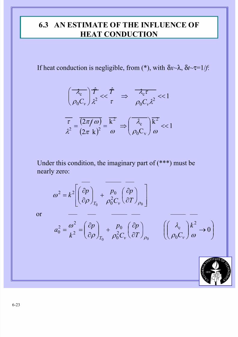
Under this condition, the imaginary part of (***) must be
nearly zero:
If heat conduction is negligible, from (*), with δ x~λ, δt ~τ=1/ f :
1ˆˆ
20
c2
0
c <<⇒<<
λ ρ
τ λ
τ λ ρ
λ
vv C
T T
C
( )
( )1
k
C
k
k 2
/2 2
v0
c2
22 <<
⇒==
ω ρ
λ
ω π
ω π
λ
τ
→
∂
∂
+
∂
∂
==
∂
∂+
∂
∂=
0
2
0
c20
02
22
0
20
022
00
00
ω ρ
λ
ρ ρ
ω
ρ ρ ω
ρ
ρ
k
C T
p
C
p p
k a
T
p
C
p pk
vvT
vT
or
6.3 AN ESTIMATE OF THE INFLUENCE OF
HEAT CONDUCTION
8/11/2019 Fundamentals of Acoustically Coupled Combustions
http://slidepdf.com/reader/full/fundamentals-of-acoustically-coupled-combustions 24/1206-24
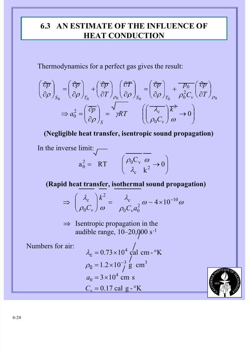
Thermodynamics for a perfect gas gives the result:
→
=
∂
∂=⇒
∂
∂+
∂
∂=
∂
∂
∂
∂+
∂
∂=
∂
∂
02
0
c20
20
0
000000
ω ρ
λ γ
ρ
ρ ρ ρ ρ ρ ρ ρ
k
C
RT p
a
T
p
C
p pT
T
p p p
vS
vT S T S
In the inverse limit:
→= 0
k
CRTa
2c
v020
ω
λ
ρ
(Rapid heat transfer, isothermal sound propagation)
Numbers for air:
K -gcal0.17
scm103
cmg101.2
K -cmcal100.73
40
33
4
°=
×=
×=
°×=
−
vC
a
0
c
ρ
λ
ω ω ρ
λ
ω ρ
λ 10
200
c2
0
c 104~ −×=
⇒
aC
k
C vv
⇒ Isentropic propagation in the
audible range, 10–20,000 s-1
(Negligible heat transfer, isentropic sound propagation)
6.3 AN ESTIMATE OF THE INFLUENCE OF
HEAT CONDUCTION
8/11/2019 Fundamentals of Acoustically Coupled Combustions
http://slidepdf.com/reader/full/fundamentals-of-acoustically-coupled-combustions 25/1206-25
6.4 ENERGY AND INTENSITY ASSOCIATED WITH
ACOUSTIC WAVES
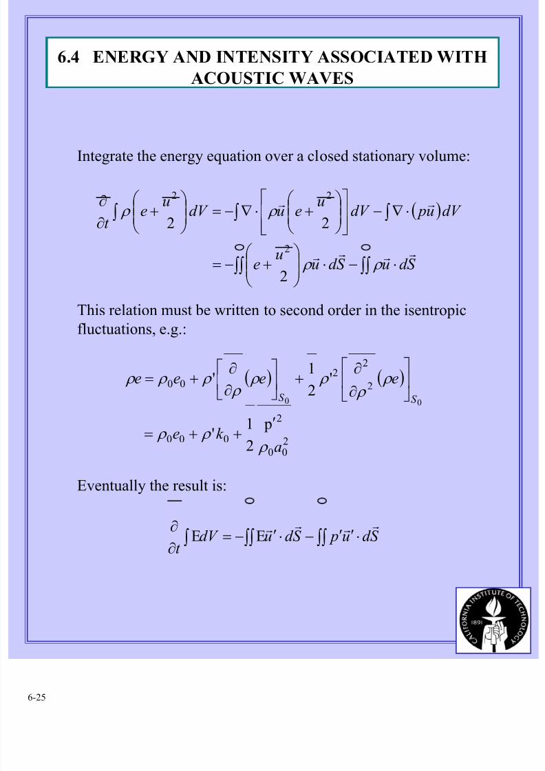
This relation must be written to second order in the isentropic
fluctuations, e.g.:
( )
∫∫∫∫
∫∫ ∫
⋅−⋅
+−=
⋅∇−
+⋅∇−=
+
∂
∂
S d uS d uu
e
dV u pdV u
eudV u
et
rrrr
rr
ρ ρ
ρ ρ
2
22
2
22
( ) ( )
200
2
000
2
22
00
p
2
1'
'
2
1'
00
ak e
eeee
S S
ρ ρ ρ
ρ
ρ
ρ ρ
ρ
ρ ρ ρ
′++=
∂
∂+
∂
∂+=
Integrate the energy equation over a closed stationary volume:
Eventually the result is:
∫∫ ∫∫∫ ⋅′′−⋅′−=∂∂ S d u pS d udV t
rrrrEE
8/11/2019 Fundamentals of Acoustically Coupled Combustions
http://slidepdf.com/reader/full/fundamentals-of-acoustically-coupled-combustions 26/1206-26
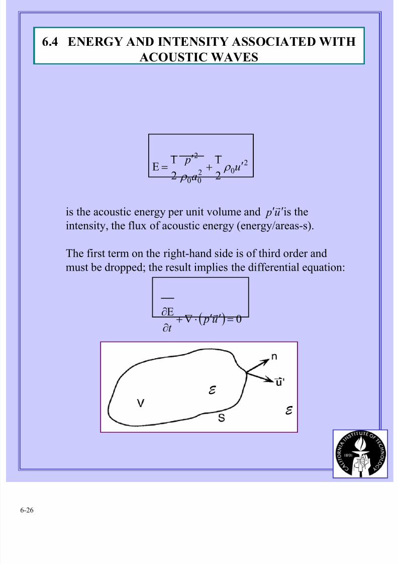
E
( ) 0=′′⋅∇+∂
∂u p
t
rE
is the acoustic energy per unit volume and is the
intensity, the flux of acoustic energy (energy/areas-s).
The first term on the right-hand side is of third order and
must be dropped; the result implies the differential equation:
u p ′′r
202
00
2
2
1
2
1u
a
p′+
′= ρ
ρ E
E
6.4 ENERGY AND INTENSITY ASSOCIATED WITH
ACOUSTIC WAVES
8/11/2019 Fundamentals of Acoustically Coupled Combustions
http://slidepdf.com/reader/full/fundamentals-of-acoustically-coupled-combustions 27/1206-27
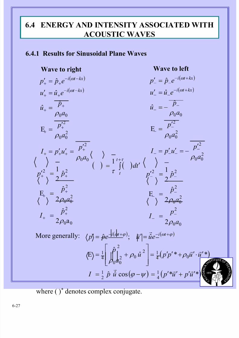
6.4.1 Results for Sinusoidal Plane Waves
Wave to right
( )
( )
00
2
200
200
ˆˆ
ˆ
ˆ
a
pu p I
a
pa
pu
euu
e p p
kxt i
kxt i
ρ
ρ
ρ
ω
ω
++++
++
++
−−++
−−++
′=′′=
′=
=
=′
=′
E
Wave to left
( )
( )
200
2
200
200
ˆˆ
ˆ
ˆ
a
pu p I
a
pa
pu
euu
e p p
kxt i
kxt i
ρ
ρ
ρ
ω
ω
−−−−
−−
−−
+−−−
+−−−
′−=′′=
′=
−=
=′
=′
E
( ) ( )∫+
′=τ
τ
t
t
t d 1
00
2
200
2
22
a2
ˆ
2
ˆ
ˆ2
1
ρ
ρ
++
++
++
=
=
=′
p I
a
p
p p
E
00
2
200
2
22
2
2
ˆ
ˆ2
1
a
p I
a
p
p p
ρ
ρ
−−
−−
−−
=
=
=′
E
More generally: ( ) ( )
( )
( ) ( )*u pu* pu p I
uu p pua
p
euue p p t it i
′′+′′=−=
′⋅′+′′=
+=
=′=′ +−+−
rrr
rr
rv
41
21
0412
0200
2
41
cosˆˆ
**ˆˆ
ˆ;ˆ
ψ ϕ
ρ ρ ρ
ϕ ω ϕ ω
E
where ( )* denotes complex conjugate.
6.4 ENERGY AND INTENSITY ASSOCIATED WITH
ACOUSTIC WAVES
8/11/2019 Fundamentals of Acoustically Coupled Combustions
http://slidepdf.com/reader/full/fundamentals-of-acoustically-coupled-combustions 28/1206-28
6.4.2 The Decay or Growth Constant
α ω ω i−→
and the variables of the motion have the behavior in time
t t -i ee α ω
where for this definition, α>0 means waves grow.
Normally in practice, |α|/ω << 1, which means that the fractional
change of amplitude is small in one cycle of the oscillation. Thus
when time averaging is carried out over one or a few cycles, e-αt isapproximately constant and the average energy is
In practice, if there is no external source of energy, waves in a
chamber will decay; or in case there are internal sources of
energy, waves may be unstable, having amplitudes growing in
time.
In ‘standing’ or ‘stationary’ waves in a chamber, the frequencyis complex
+=
2
0200
2
t ˆˆ
4
1u
a
pe ρ
ρ
α E
6.4 ENERGY AND INTENSITY ASSOCIATED WITH
ACOUSTIC WAVES
8/11/2019 Fundamentals of Acoustically Coupled Combustions
http://slidepdf.com/reader/full/fundamentals-of-acoustically-coupled-combustions 29/1206-29
6.4.2 The Decay or Growth Constant (cont’d)
Hence we have the important interpretations of α which serve
as the basis for measuring α:
dt
d
dt
pd
p
E
E
12
ˆ
ˆ
1
=
=
α
α
Note: the sign of α is a matter of definition.
6.4 ENERGY AND INTENSITY ASSOCIATED WITH
ACOUSTIC WAVES
8/11/2019 Fundamentals of Acoustically Coupled Combustions
http://slidepdf.com/reader/full/fundamentals-of-acoustically-coupled-combustions 30/1206-30
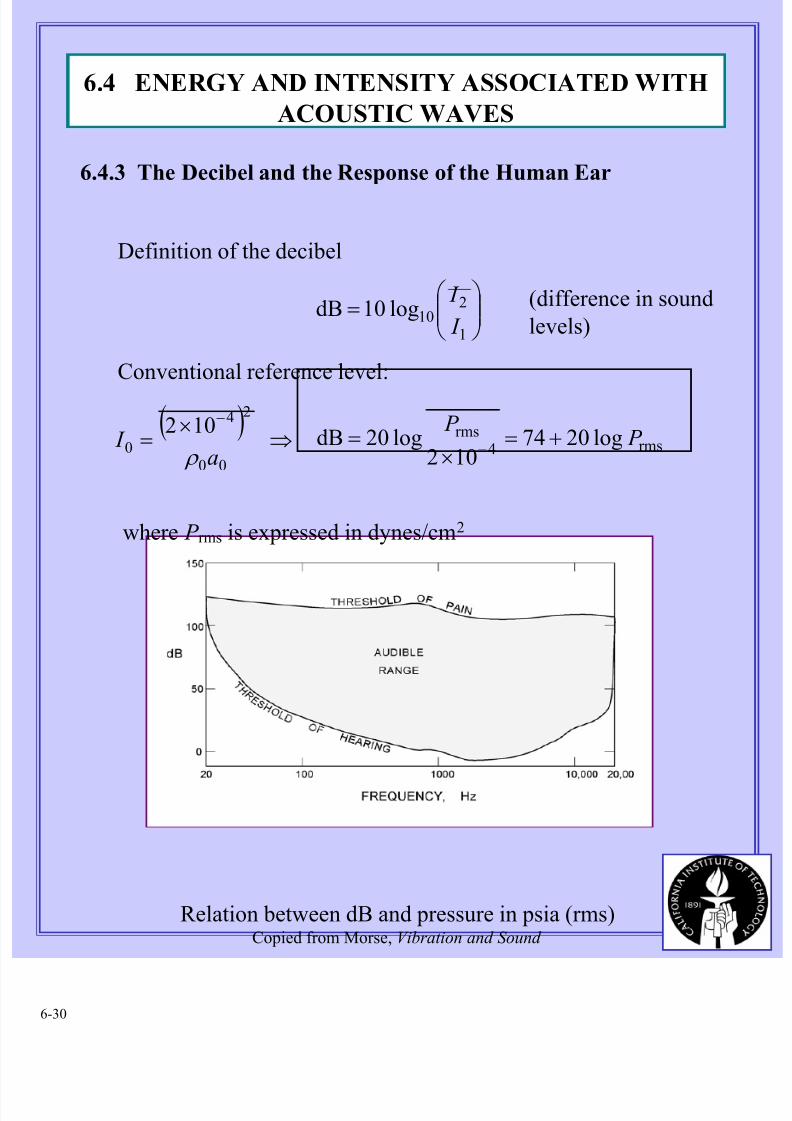
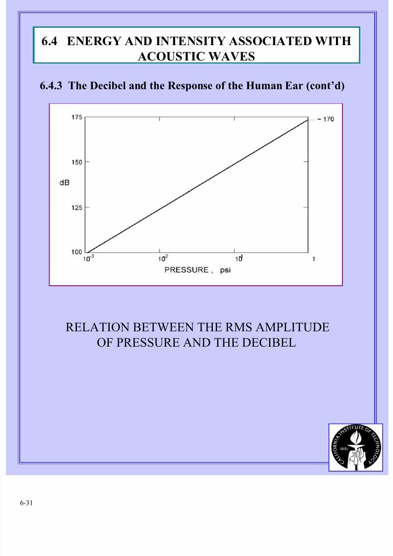
6.4.3 The Decibel and the Response of the Human Ear
rms4rms log2074102
log20dB P P
+=×
=−
=
1
210log10dB
I
I
Conventional reference level:
( )
102
00
24
0 ⇒×
=−
a I
ρ
(difference in sound
levels)
where P rms is expressed in dynes/cm2
Definition of the decibel
Relation between dB and pressure in psia (rms)Copied from Morse, Vibration and Sound
6.4 ENERGY AND INTENSITY ASSOCIATED WITH
ACOUSTIC WAVES
8/11/2019 Fundamentals of Acoustically Coupled Combustions
http://slidepdf.com/reader/full/fundamentals-of-acoustically-coupled-combustions 31/1206-31
RELATION BETWEEN THE RMS AMPLITUDE
OF PRESSURE AND THE DECIBEL
6.4 ENERGY AND INTENSITY ASSOCIATED WITH
ACOUSTIC WAVES
6.4.3 The Decibel and the Response of the Human Ear (cont’d)
8/11/2019 Fundamentals of Acoustically Coupled Combustions
http://slidepdf.com/reader/full/fundamentals-of-acoustically-coupled-combustions 32/1206-32
6.5 BOUNDARY CONDITIONS; REFLECTIONS
FROM A SURFACE
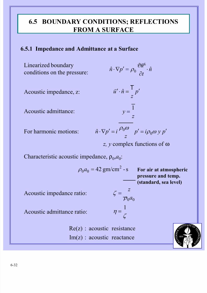
6.5.1 Impedance and Admittance at a Surface
Linearized boundary
conditions on the pressure:
Acoustic impedance, z:
Acoustic admittance:
For harmonic motions:
z, y complex functions of ω
nt
u pn ˆˆ 0 ⋅
∂
′∂=′∇⋅
r
ρ
p z
nu ′=⋅′1
ˆr
p yi p z
i pn ′=′=′∇⋅ ω ρ ω ρ
00ˆ
z y
1=
Characteristic acoustic impedance, ρ0,a0:
s-gm/cm42 200 =a ρ
Acoustic impedance ratio:
00a
z
ρ ζ =
Acoustic admittance ratio:ζ
η 1
=
reactanceacoustic :Im(z)
resistanceacoustic :Re(z)
For air at atmospheric
pressure and temp.
(standard, sea level)
8/11/2019 Fundamentals of Acoustically Coupled Combustions
http://slidepdf.com/reader/full/fundamentals-of-acoustically-coupled-combustions 33/1206-33
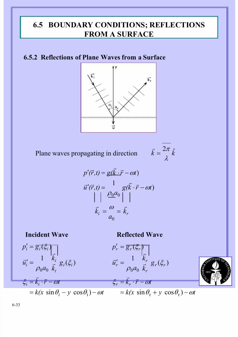
6.5.2 Reflections of Plane Waves from a Surface
Plane waves propagating in direction k k ˆ2
λ
π =
r
)1
)
00
t r k g( a
,t)r ( u
t r k g( ,t)r ( p
ω ρ
ω
−⋅=′
−⋅=′rrrr
rrr
t yk(x
t r k
g k
k
au
g p
i
ii
ii
i
ii
iii
ω θ θ
ω ξ
ξ ρ
ξ
−−=
−⋅=
=′
=′
)cossin
)(1
)(
i
00
rr
r
rr
r i k a
k rr
==0
ω
Incident Wave Reflected Wave
t yk(x
t r k
g k
k
au
g p
r r
r r
r
r r
r r r
ω θ θ
ω ξ
ξ ρ
ξ
−+=
−⋅=
=′
=′
)cossin
)(1
)(
r r
00
rr
r
rr
6.5 BOUNDARY CONDITIONS; REFLECTIONS
FROM A SURFACE
8/11/2019 Fundamentals of Acoustically Coupled Combustions
http://slidepdf.com/reader/full/fundamentals-of-acoustically-coupled-combustions 34/1206-34
6.5.2 Reflections of Plane Waves from a Surface (cont’d)
Surface Impedance
)sin(cos)sin(cos
t)sin()sin(00
0t kx g t kx g
kx g t kx g a
u
p z
r r r iii
r r ii
y y ω θ θ ω θ θ
ω θ ω θ ρ
−+−−
−+−=
′−
′=−
=
In general: z(x) z =
Assume z independent of x: True if ( ) ( )
=
==
ξ β ξ
θ θ θ
ir
ir
g g
( ) θ β
β ρ
cos1
100
+−
+=−⇒ a z
Reflection coefficient:00
00
cos
cos
a z
a z
ρ θ
ρ θ β
+
−=
E.g. θ = 0: no reflection if z = ρ0a0
(perfect impedance matching)
θ ≠ 0: non-zero reflection (!)
Nonsense: because the transmitted wave,
required to conserve energy, has not been
accounted for
⇒ the result is not valid for z = ρ0a0
6.5 BOUNDARY CONDITIONS; REFLECTIONS
FROM A SURFACE
8/11/2019 Fundamentals of Acoustically Coupled Combustions
http://slidepdf.com/reader/full/fundamentals-of-acoustically-coupled-combustions 35/1206-35
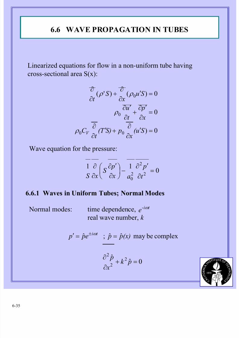
6.6 WAVE PROPAGATION IN TUBES
0)
0
0)()'(
00
0
0
=′∂
∂+′
∂
∂
=∂
′∂+
∂
′∂
=′∂
∂+
∂
∂
S u( x
pS)T ( t
C
x
p
t
u
S u x
S t
V ρ
ρ
ρ ρ
Linearized equations for flow in a non-uniform tube having
cross-sectional area S(x):
t ie ω -
Wave equation for the pressure:
6.6.1 Waves in Uniform Tubes; Normal Modes
Normal modes: time dependence,
real wave number, k
0
11
2
2
20
=∂
′∂−
∂
′∂
∂
∂
t
p
a x
p
S xS
complex bemayˆˆ; ˆ (x) p pe p p t i ==′ ± ω
0ˆˆ 2
2
2
=+∂
∂ pk
x
p
8/11/2019 Fundamentals of Acoustically Coupled Combustions
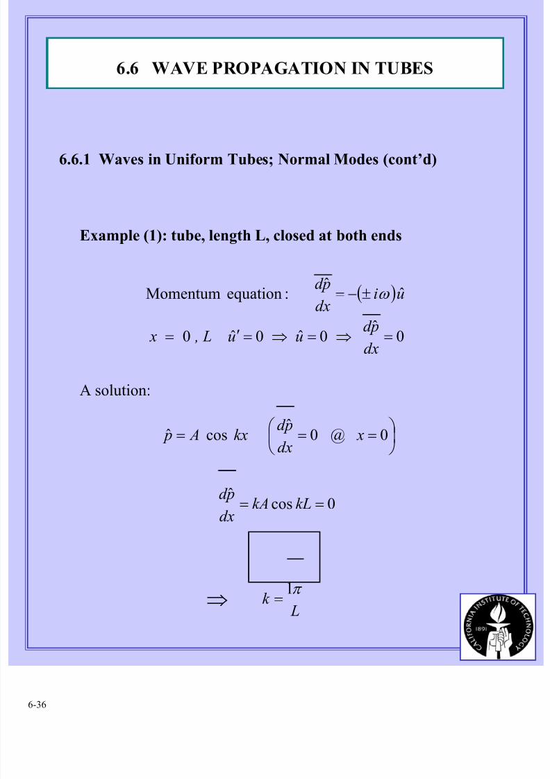
http://slidepdf.com/reader/full/fundamentals-of-acoustically-coupled-combustions 36/1206-36
( )
0ˆ
0ˆ0ˆ0
ˆˆ
:equation Momentum
=⇒=⇒=′=
±−=
dx
pd uu , L x
uidx
pd ω
Example (1): tube, length L, closed at both ends
A solution:
6.6.1 Waves in Uniform Tubes; Normal Modes (cont’d)
=== 00
ˆcosˆ @ x
dx
pd kx A p
0cosˆ
== kLkAdx
pd
⇒ L
k π l
=
6.6 WAVE PROPAGATION IN TUBES
8/11/2019 Fundamentals of Acoustically Coupled Combustions
http://slidepdf.com/reader/full/fundamentals-of-acoustically-coupled-combustions 37/1206-37
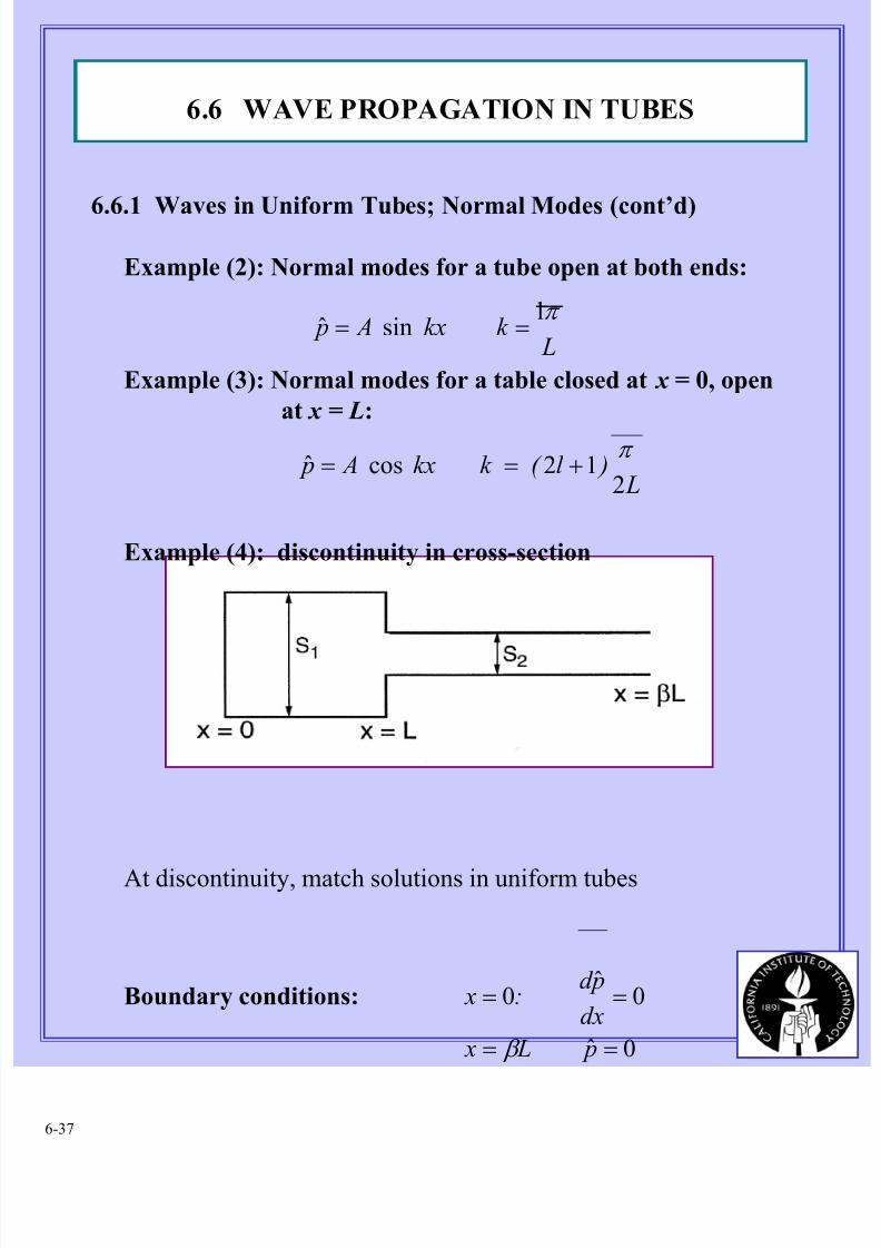
Example (2): Normal modes for a tube open at both ends:
Example (3): Normal modes for a table closed at x = 0, open
at x = L:
6.6.1 Waves in Uniform Tubes; Normal Modes (cont’d)
L )l ( kkx A p
212cosˆ
π +==
Lk kx A p
π l sinˆ ==
0ˆ
0ˆ
0
==
==
p L x
dx
pd : x
β
Example (4): discontinuity in cross-section
At discontinuity, match solutions in uniform tubes
Boundary conditions:
6.6 WAVE PROPAGATION IN TUBES
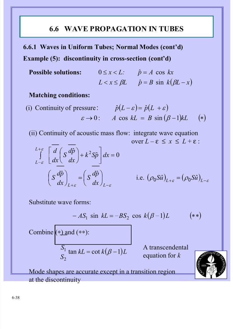
8/11/2019 Fundamentals of Acoustically Coupled Combustions
http://slidepdf.com/reader/full/fundamentals-of-acoustically-coupled-combustions 38/1206-38
( ) x Lk B p L x L
kx A p L: x
−=≤<
=<≤
β β sinˆ
cosˆ0
Example (5): discontinuity in cross-section (cont’d)
(ii) Continuity of acoustic mass flow: integrate wave equation
over L – ε ≤ x ≤ L + ε :
Possible solutions:
Matching conditions:
( ) ( )
( ) ( )∗−=→
+=−
:
1sincos :0
ˆˆ pressureof Continuity (i)
kL BkL A
L p L p
β ε
ε ε
0ˆˆ
2 =
+
∫
+
−
dx pS k dx
pd S
dx
d L
L
ε
ε
( ) ( )ˆˆi.e.ˆˆ
ε ε ε ε
ρ ρ −+−+
=
=
L L
L L
uS uS dx
pd S
dx
pd S 00
Substitute wave forms:
( ) ( )∗∗−−=− Lk BS kL AS 1cossin 21 β
Combine (∗) and (∗∗):
( ) Lk kLS
S 1cottan
2
1 −= β A transcendental
equation for k
Mode shapes are accurate except in a transition region
at the discontinuity
6.6 WAVE PROPAGATION IN TUBES
6.6.1 Waves in Uniform Tubes; Normal Modes (cont’d)
8/11/2019 Fundamentals of Acoustically Coupled Combustions
http://slidepdf.com/reader/full/fundamentals-of-acoustically-coupled-combustions 39/1206-39
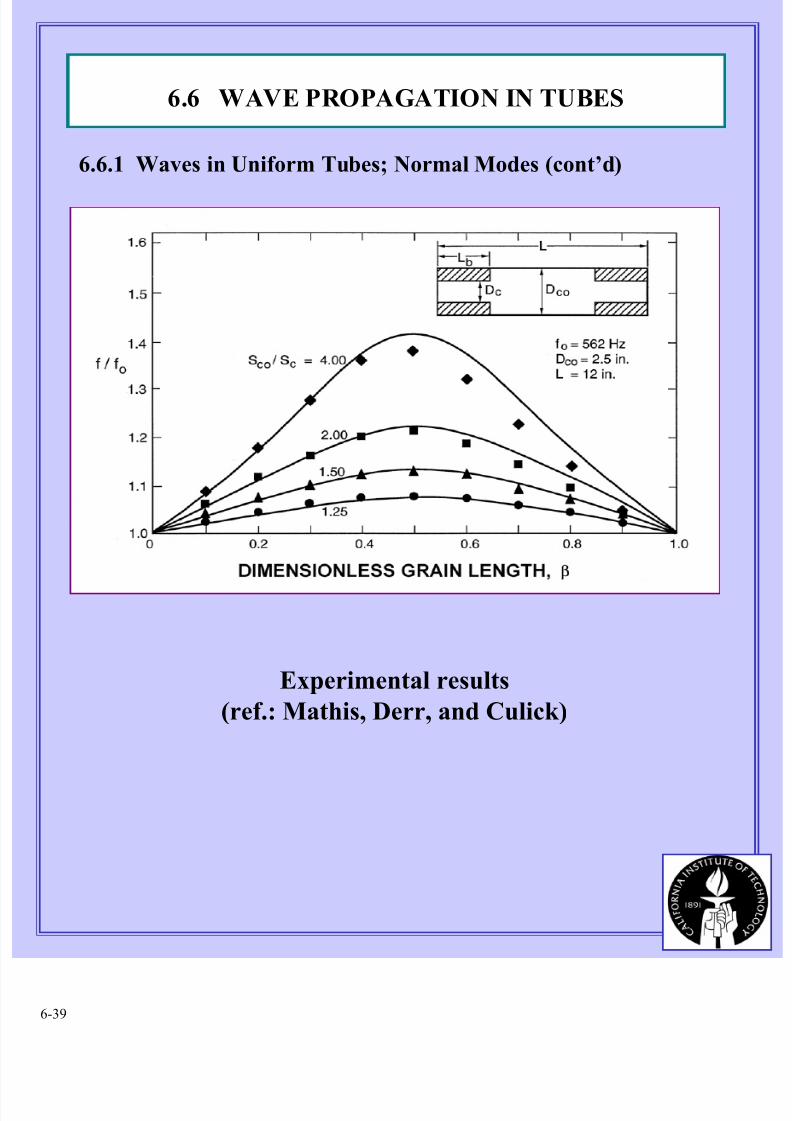
Experimental results
(ref.: Mathis, Derr, and Culick)
6.6 WAVE PROPAGATION IN TUBES
6.6.1 Waves in Uniform Tubes; Normal Modes (cont’d)
8/11/2019 Fundamentals of Acoustically Coupled Combustions
http://slidepdf.com/reader/full/fundamentals-of-acoustically-coupled-combustions 40/1206-40
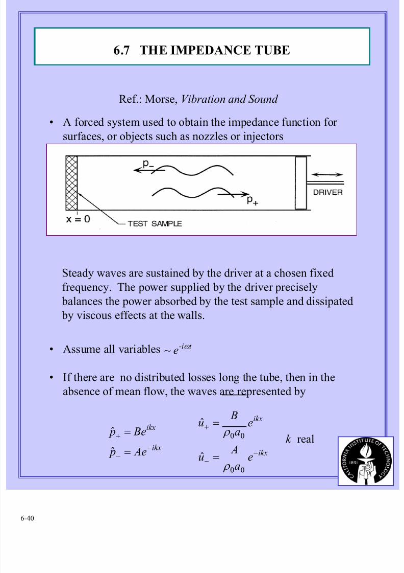
6.7 THE IMPEDANCE TUBE
Ref.: Morse, Vibration and Sound
• A forced system used to obtain the impedance function for
surfaces, or objects such as nozzles or injectors
Steady waves are sustained by the driver at a chosen fixed
frequency. The power supplied by the driver precisely
balances the power absorbed by the test sample and dissipated
by viscous effects at the walls.
• Assume all variables
• If there are no distributed losses long the tube, then in the
absence of mean flow, the waves are represented by
t -ie~ ω
ikx
ikx
Ae p
Be p
−−
+
=
=
ˆ
ˆ
ikx
ikx
ea
Au
ea
Bu
−−
+
=
=
00
00
ˆ
ˆ
ρ
ρ real k
8/11/2019 Fundamentals of Acoustically Coupled Combustions
http://slidepdf.com/reader/full/fundamentals-of-acoustically-coupled-combustions 41/1206-41
Impedance at z = 0:
002 i 0 πβ πα ψ +=−== Ae: B z
( )( )00
002
2
2
000 /1
/1
1
1
ˆ
ˆ
a z
a z e
e
ea
u
p z
x ρ
ρ ρ ψ
ψ
ψ
+
−=
+
−=
−=
=
[ ]ψ
ψ
ρ
2
00
2
ˆ
ˆ
+−
+−
+−=
−=
ikxikx
ikxikx
eea
Au
ee A p
Values of ψ = π α0 + i π β0 are inferred frommeasurements of the envelope of the modal structure
along the impedance tube
( ) ( )ikxk Aeee Ae x p ikxikx +−=−−= −−+ψ ψ ψ ψ ψ sin2ˆ
( )
+=
=
+=+λ
β β
α α
β α π ψ xiikx 20
0
( ) πβ πα β α π πα ψ coscosh2sin2ˆ 22 −=+= Aeik e A p
6.7 THE IMPEDANCE TUBE
8/11/2019 Fundamentals of Acoustically Coupled Combustions
http://slidepdf.com/reader/full/fundamentals-of-acoustically-coupled-combustions 42/1206-42
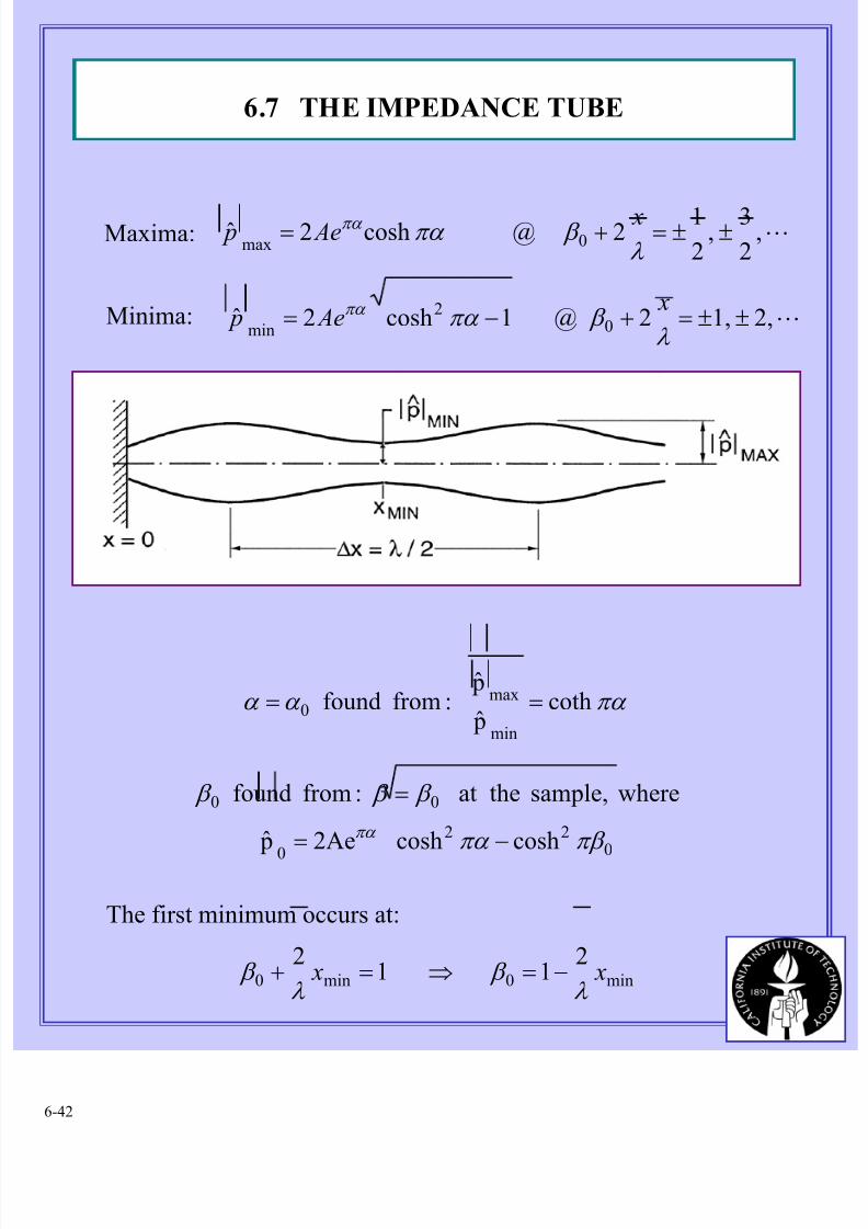
Maxima: L,2
3 ,
2
12 @ cosh2ˆ 0max
±±=+=λ
β πα πα x Ae p
Minima: L2,1,2 @ 1cosh2ˆ 02
min ±±=+−=
λ β πα πα x
Ae p
πα α α coth p
p :from found
min
max0 ==
022
0
00
coshcosh2Ae p
wheresample, at the :from found
πβ πα
β β β
πα
−=
=
The first minimum occurs at:
min0min0
21 1
2 x x
λ β
λ β −=⇒=+
6.7 THE IMPEDANCE TUBE
8/11/2019 Fundamentals of Acoustically Coupled Combustions
http://slidepdf.com/reader/full/fundamentals-of-acoustically-coupled-combustions 43/1206-43
6.8 VISCOUS LOSSES AT AN INERT SURFACE
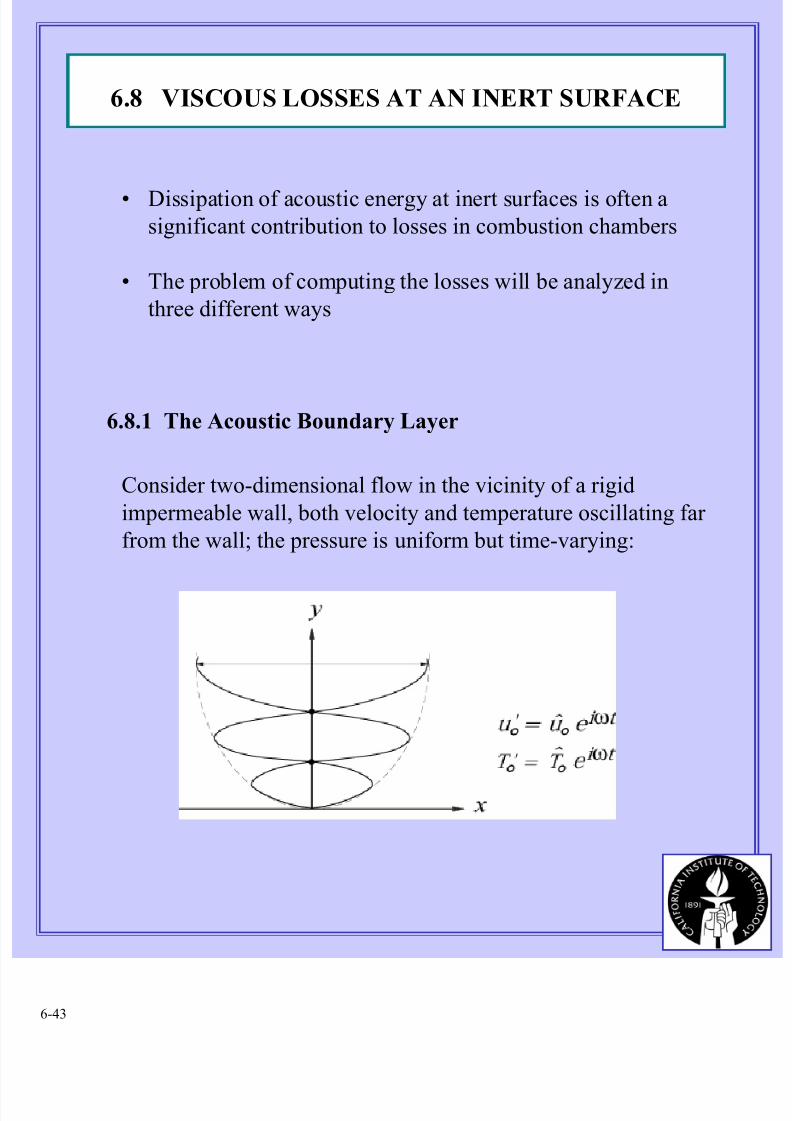
• Dissipation of acoustic energy at inert surfaces is often asignificant contribution to losses in combustion chambers
• The problem of computing the losses will be analyzed in
three different ways
Consider two-dimensional flow in the vicinity of a rigid
impermeable wall, both velocity and temperature oscillating far
from the wall; the pressure is uniform but time-varying:
6.8.1 The Acoustic Boundary Layer
8/11/2019 Fundamentals of Acoustically Coupled Combustions
http://slidepdf.com/reader/full/fundamentals-of-acoustically-coupled-combustions 44/1206-44
0'
0 =
∂
′∂+
∂
′∂+
∂
∂
x
u
y
v
t ρ
ρ
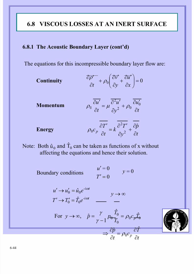
6.8.1 The Acoustic Boundary Layer (cont’d)
The equations for this incompressible boundary layer flow are:
Continuity
Momentum
Energy
t
u
y
u
t
u
∂
′∂+
∂
′∂=
∂
′∂ 002
2
0 ρ µ ρ
t
p
y
T k
t
T c p
∂
∂+
∂
′∂=
∂
′∂ ˆ2
2
0 ρ
Note: Both and can be taken as functions of x without
affecting the equations and hence their solution.0u 0T
Boundary conditions0
0
=′
=′
T
u0= y
t -i
t -i
eT T T
euuu
ω
ω
00
00
ˆ
ˆ
=′→′
=′→′ ∞→ y
t
T
ct
p
T cT
T p p y
p
p
∂
∂
=∂
∂
⇒
=−
=∞→
ˆˆ
ˆˆ
1ˆ ,For
0
000
00
ρ
ρ γ
γ
6.8 VISCOUS LOSSES AT AN INERT SURFACE
8/11/2019 Fundamentals of Acoustically Coupled Combustions
http://slidepdf.com/reader/full/fundamentals-of-acoustically-coupled-combustions 45/1206-45
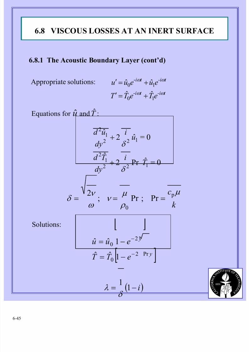
6.8.1 The Acoustic Boundary Layer (cont’d)
Appropriate solutions:
t -it i
t -it i
eT eT T
eueuu
ω ω
ω ω
1-
0
1-
0
ˆˆ
ˆˆ
+=′
+=′
Equations for and :u T
0=ˆPr 2ˆ
0=ˆ2ˆ
1221
2
1221
2
T i
dy
T d
ui
dy
ud
δ
δ
+
+
Solutions:
k
c µ
ρ
µ ν
ω
ν δ
p
0
Pr ;Pr ;2
===
[ ] y
y
eT T
euuPr 2
0
20
1ˆˆ
1ˆˆ−
−
−=−=
( )i−= 11
δ λ
6.8 VISCOUS LOSSES AT AN INERT SURFACE
8/11/2019 Fundamentals of Acoustically Coupled Combustions
http://slidepdf.com/reader/full/fundamentals-of-acoustically-coupled-combustions 46/1206-46
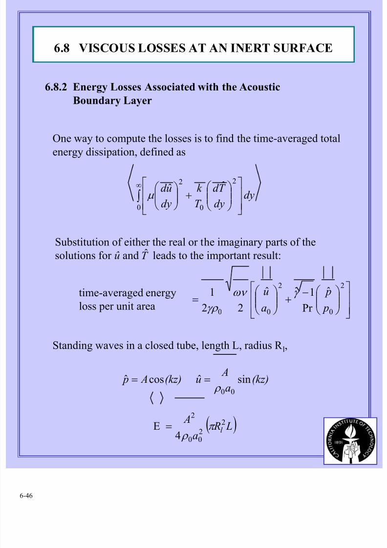
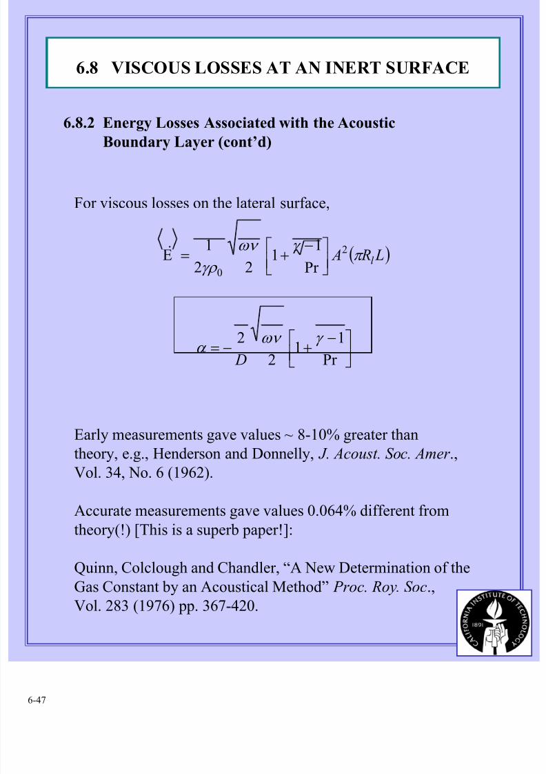
6.8.2 Energy Losses Associated with the Acoustic
Boundary Layer
One way to compute the losses is to find the time-averaged total
energy dissipation, defined as
∫∞
+
0
2
0
2
ˆˆ dydyT d
T k
dyud µ
Substitution of either the real or the imaginary parts of the
solutions for û and leads to the important result:T
−+
=
2
0
2
00
ˆ
Pr
1ˆ
22
1
p
p
a
u γ ων
γρ
time-averaged energy
loss per unit area
Standing waves in a closed tube, length L, radius R l,
(kz)a
Au(kz) A p sinˆcosˆ00 ρ
==
( ) L Ra
Al 2
200
2
4π
ρ =E
6.8 VISCOUS LOSSES AT AN INERT SURFACE
8/11/2019 Fundamentals of Acoustically Coupled Combustions
http://slidepdf.com/reader/full/fundamentals-of-acoustically-coupled-combustions 47/120
8/11/2019 Fundamentals of Acoustically Coupled Combustions
http://slidepdf.com/reader/full/fundamentals-of-acoustically-coupled-combustions 48/1206-48
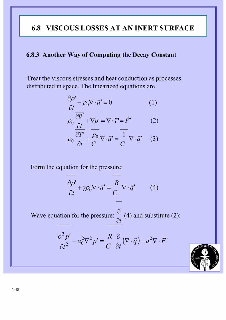
6.8.3 Another Way of Computing the Decay Constant
Treat the viscous stresses and heat conduction as processes
distributed in space. The linearized equations are
(3)1
(2)'
(1)0'
00
0
0
qC
uC
p
t
T
F pt
u
u
t
′⋅∇=′⋅∇+∂
′∂
′=⋅∇=′∇+∂
′∂
=′⋅∇+
∂
∂
rr
rtr
r
ρ
τ ρ
ρ ρ
Form the equation for the pressure:
(4)'
0 qC
Ru
t ′⋅∇=′⋅∇+
∂
∂ rrγρ
ρ
Wave equation for the pressure: (4) and substitute (2):t ∂
∂
( ) F aqt C
R pa
t
p′⋅∇−⋅∇
∂
∂=′∇−
∂
′∂ rr 22202
2
6.8 VISCOUS LOSSES AT AN INERT SURFACE
8/11/2019 Fundamentals of Acoustically Coupled Combustions
http://slidepdf.com/reader/full/fundamentals-of-acoustically-coupled-combustions 49/1206-49
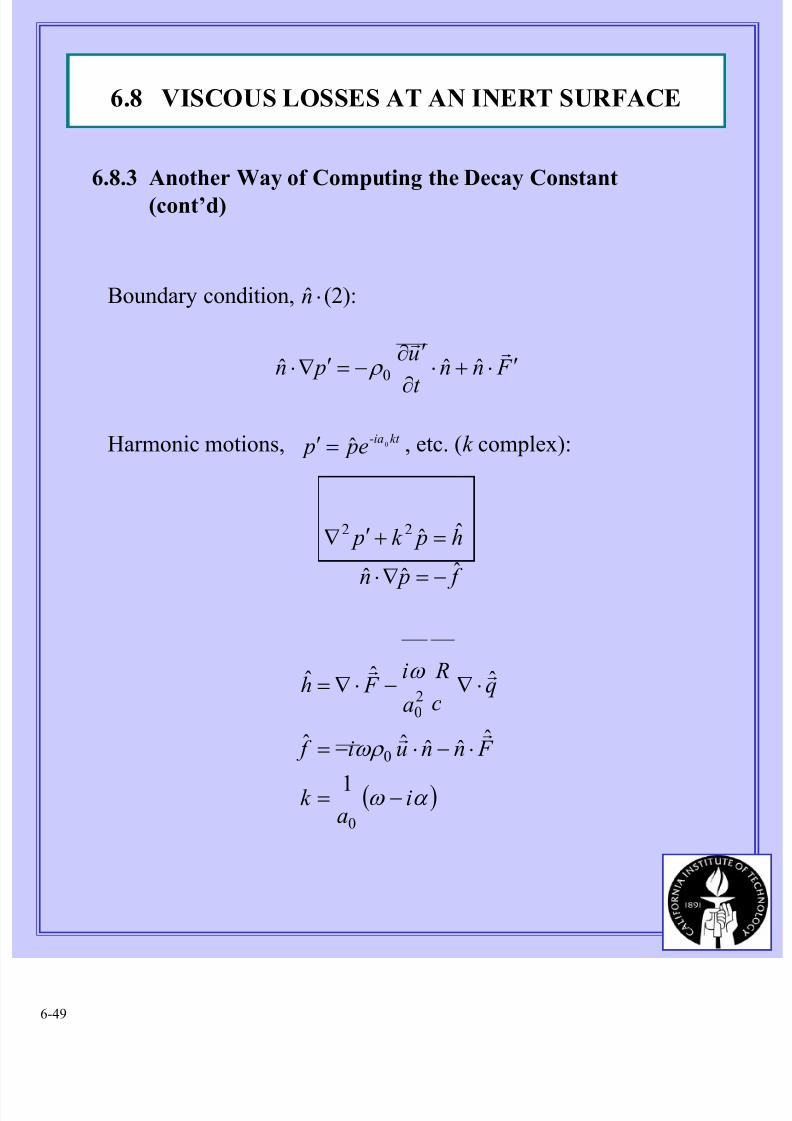
6.8.3 Another Way of Computing the Decay Constant
(cont’d)
Boundary condition, (2):⋅n
F nnt
u pn ′⋅+⋅
∂
′∂−=′∇⋅
rrˆˆˆ 0 ρ
Harmonic motions, , etc. (k complex):kt -iae p p 0ˆ=′
f pn
h pk p
ˆˆˆ
ˆˆ22
−=∇⋅
=+′∇
( )α ω
ωρ
ω
ia
k
F nnui f
qc
R
a
i F h
−=
⋅−⋅−=
⋅∇−⋅∇=
0
0
20
1
ˆˆˆˆˆ
ˆˆˆ
rr
rr
6.8 VISCOUS LOSSES AT AN INERT SURFACE
8/11/2019 Fundamentals of Acoustically Coupled Combustions
http://slidepdf.com/reader/full/fundamentals-of-acoustically-coupled-combustions 50/120
8/11/2019 Fundamentals of Acoustically Coupled Combustions
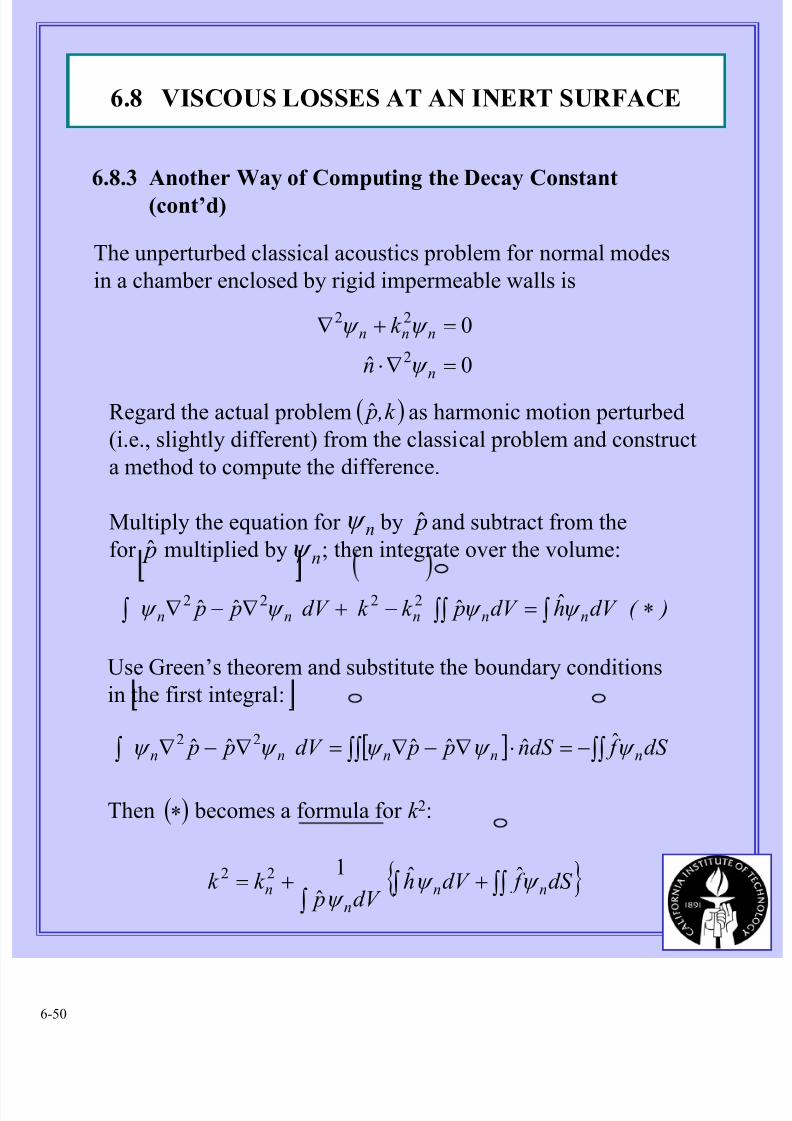
http://slidepdf.com/reader/full/fundamentals-of-acoustically-coupled-combustions 51/1206-51
6.8.3 Another Way of Computing the Decay Constant
(cont’d)
{ }∫ ∫∫++= dS f dV h E
k k nn
n
n ψ ψ ˆˆ12
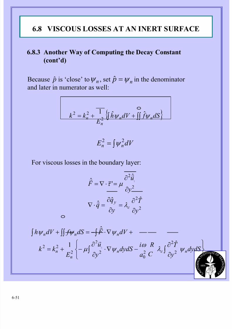
22
Because is ‘close’ to , set in the denominator
and later in numerator as well:
p nψ
∫= dV E nn22 ψ
For viscous losses in the boundary layer:
2
2
2
2
ˆˆˆ
ˆ'
ˆ
y
T
y
y
u F
c y
||
∂
∂=
∂
∂=⋅∇
∂
∂=⋅∇=
λ
µ τ
r
rtr
∂
∂−∇⋅
∂
∂−+=
+∇⋅−=+
∫∫
∫∫ ∫∫
dydS y
T
C
R
a
idydS
y
u
E k k
dV F dS f dV h
ncn
n
n
nnn
|| ψ λ ω
ψ µ
ψ ψ ψ
2
2
20
2
2
2
22ˆ1
ˆ
r
r
6.8 VISCOUS LOSSES AT AN INERT SURFACE
n p ψ =ˆ
8/11/2019 Fundamentals of Acoustically Coupled Combustions
http://slidepdf.com/reader/full/fundamentals-of-acoustically-coupled-combustions 52/120
8/11/2019 Fundamentals of Acoustically Coupled Combustions
http://slidepdf.com/reader/full/fundamentals-of-acoustically-coupled-combustions 53/1206-53
6.9 PROPAGATION OF HIGHER-ORDER MODES IN
TUBES
The behavior discussed in this section is included partly
as an example of departures from the purely one-dimensional
wave propagation assumed in most of the preceding analyses;
and partly because the results are applicable to slender
passages in combustion; i.e. regions having relative large
values of length/transverse dimension.
6.9.1 Traveling Plane Waves and Reflections in a Duct
If the frequency of a wave traveling along the axis of a rectangular
tube is larger than the speed of sound divided by twice the largest
lateral dimension of the tube, then the motion cannot be treated as
perfectly parallel to the axis. That frequency is called the “cut-off”
frequency, f c.
For f > f c, modes other than the simple one-dimensional
mode will propagate in the duct, i.e. purely axial waves lie in the
region of lower frequencies.
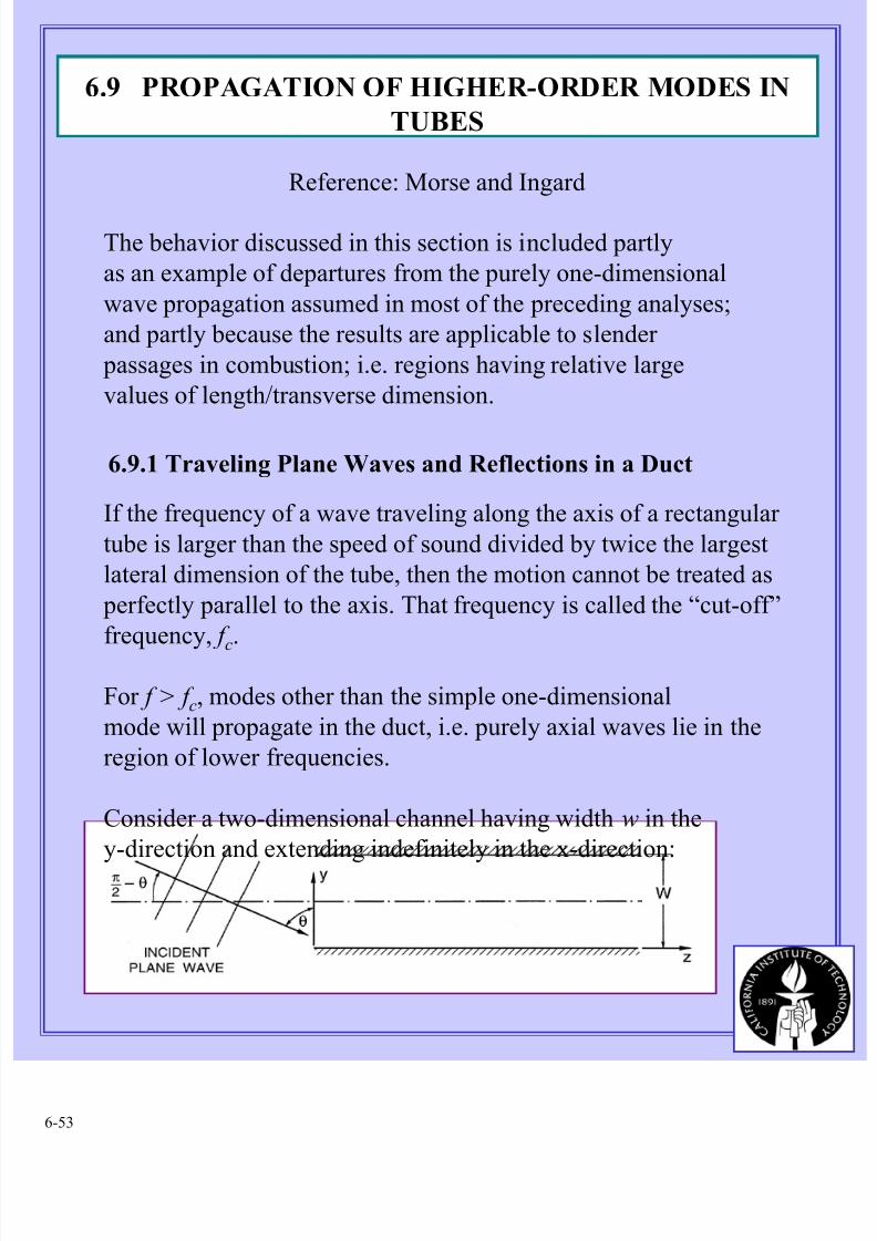
Consider a two-dimensional channel having width w in the
y-direction and extending indefinitely in the x-direction:
Reference: Morse and Ingard
8/11/2019 Fundamentals of Acoustically Coupled Combustions
http://slidepdf.com/reader/full/fundamentals-of-acoustically-coupled-combustions 54/1206-54
and the corresponding wavelength is 2w, the wavelength for the fundamental standing wave for motions normal to the axis
For f > f c, purely one-dimensional waves will propagate in
principle; for the higher frequencies interesting things are
possible, namely wave structure in transverse planes.
Consider a plane wave incident at angle to the axis onthe entrance to the tube.
6.9.1 Traveling Plane Waves and Reflections in a Duct (cont’d)
For the case illustrated, the cut-off frequency is exactly
w
a f c
2
0=
θ π −2 /
What gets through the tube?
Answering the question requires treating reflections from the
walls of the tube.
First treat reflection from a rigid surface: 0ˆ =⋅′ nur
6.9 PROPAGATION OF HIGHER-ORDER MODES IN
TUBES
8/11/2019 Fundamentals of Acoustically Coupled Combustions
http://slidepdf.com/reader/full/fundamentals-of-acoustically-coupled-combustions 55/1206-55
The surface impedance is infinitely large and the reflection
coefficient β = 1 (§5.5). Hence
g g g r i ==
and the velocity component normal to the wall is:
( ) ( )[ ]
( ){ } ( ){ }[ ]t y z k g t y z k g a
g g a
v r r ii
ω θ θ ω θ θ ρ
ξ ξ ρ
−+−−−−=
+−=
cossincossincos
cos
00
00
For sinusoidal waves, ( ) : Ae g iξ ξ =
[ ]
( ) t)i(kz
kyikyit)i(kz
ekya
iA
eeea
Av
ω θ
θ θ ω θ
θ ρ
θ
ρ
θ
−
−−−
=
−−=
sin
00
coscossin
00
cossincos
2
cos
6.9 PROPAGATION OF HIGHER-ORDER MODES IN
TUBES
6.9.1 Traveling Plane Waves and Reflections in a Duct (cont’d)
8/11/2019 Fundamentals of Acoustically Coupled Combustions
http://slidepdf.com/reader/full/fundamentals-of-acoustically-coupled-combustions 56/1206-56
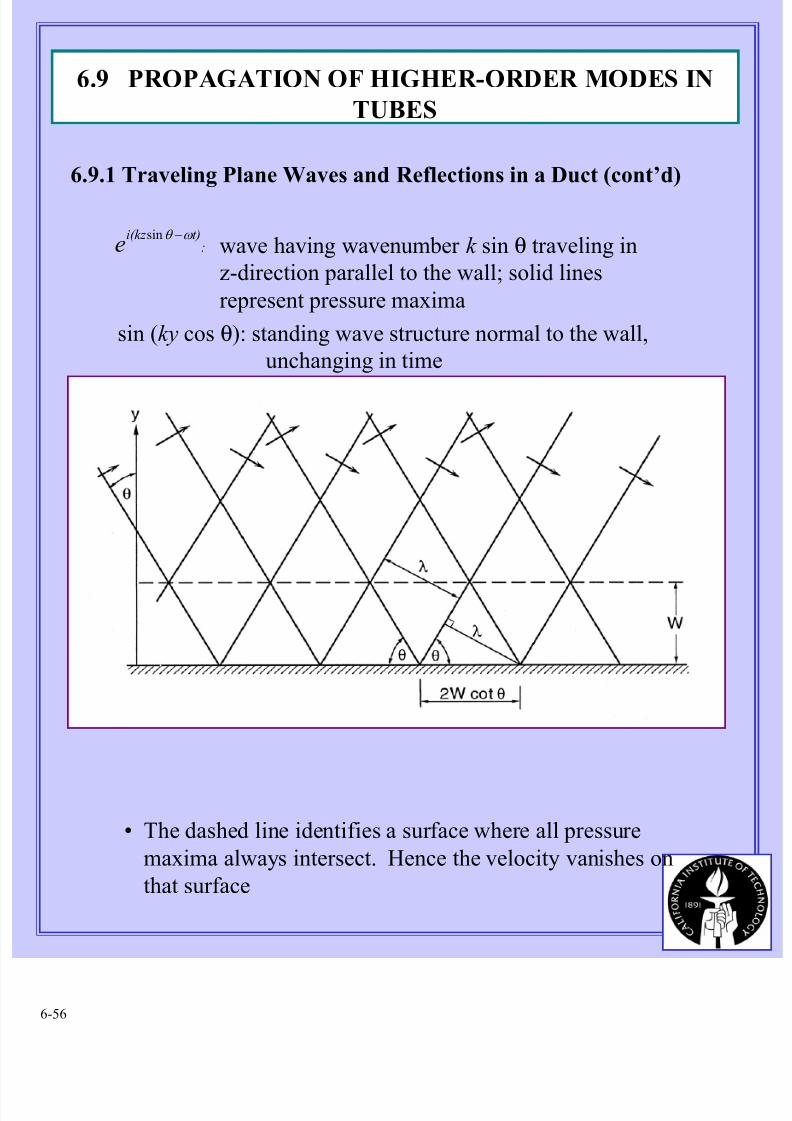
:t)i(kz
e ω θ −sin
wave having wavenumber k sin θ traveling in
z-direction parallel to the wall; solid lines
represent pressure maxima
sin (ky cos θ): standing wave structure normal to the wall,
unchanging in time
• The dashed line identifies a surface where all pressure
maxima always intersect. Hence the velocity vanishes on
that surface
6.9 PROPAGATION OF HIGHER-ORDER MODES IN
TUBES
6.9.1 Traveling Plane Waves and Reflections in a Duct (cont’d)
8/11/2019 Fundamentals of Acoustically Coupled Combustions
http://slidepdf.com/reader/full/fundamentals-of-acoustically-coupled-combustions 57/1206-57
only for particular values of ωW.
This condition defines “higher order modes” for
propagation in a tube or duct.
A Plane Wave Reflecting from a Rigid Surface
The velocity vanishes on all planes such that
( ) 0cossin =θ ky
In particular, on the surface y = W , the normal velocity vanishes
if the frequency has the values given byk a0=ω
0cossin0
=
θ
ω
a
W
Wave propagates parallel to the wall, the velocity
is parallel to the wall and for all
W and ω.
0cossin0
=
θ
ω
a
W :2/π θ =
:2/π θ < 0cossin0
=
θ ω
aW
6.9 PROPAGATION OF HIGHER-ORDER MODES IN
TUBES
6.9.1 Traveling Plane Waves and Reflections in a Duct (cont’d)
8/11/2019 Fundamentals of Acoustically Coupled Combustions
http://slidepdf.com/reader/full/fundamentals-of-acoustically-coupled-combustions 58/1206-58
( for waves incident from the left)
Cut-off Frequency
Fix W ; then requires0cossin0
=
θ
ω
a
W
π θ
ω
l a
W
=
cos
0
or
W l
W
al
2cos 0 λ
ω π θ ==
20 / π θ ≤≤
Special cases:
l = 0:
l = 1:
2
π θ = and motions are one-dimensional
parallel to the surface,
0
sina
k k ω
θ ==
W
a
W
a 00 1cos π ω ω
π θ ≥⇒≤=
Critical or ‘cut-off’ value is
W a
W
a
c
c
22 0
0
==
=
ω π λ
π ω
6.9 PROPAGATION OF HIGHER-ORDER MODES IN
TUBES
6.9.1 Traveling Plane Waves and Reflections in a Duct (cont’d)
8/11/2019 Fundamentals of Acoustically Coupled Combustions
http://slidepdf.com/reader/full/fundamentals-of-acoustically-coupled-combustions 59/1206-59
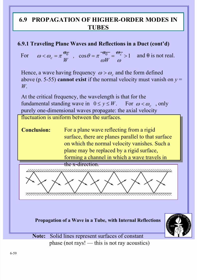
For and θ is not real.1cos 00 >===<ω
ω
ω π θ π ω ω c
cW
a ,
W
a
Hence, a wave having frequency and the form defined
above (p. 5-55) cannot exist if the normal velocity must vanish on y =
W .
At the critical frequency, the wavelength is that for thefundamental standing wave in For , only
purely one-dimensional waves propagate: the axial velocity
fluctuation is uniform between the surfaces.
cω ω >
.0 W y ≤≤
Conclusion: For a plane wave reflecting from a rigid
surface, there are planes parallel to that surface
on which the normal velocity vanishes. Such a plane may be replaced by a rigid surface,
forming a channel in which a wave travels in
the x-direction.
Propagation of a Wave in a Tube, with Internal Reflections
Note: Solid lines represent surfaces of constant
phase (not rays! — this is not ray acoustics)
cω ω <
6.9 PROPAGATION OF HIGHER-ORDER MODES IN
TUBES
6.9.1 Traveling Plane Waves and Reflections in a Duct (cont’d)
8/11/2019 Fundamentals of Acoustically Coupled Combustions
http://slidepdf.com/reader/full/fundamentals-of-acoustically-coupled-combustions 60/1206-60
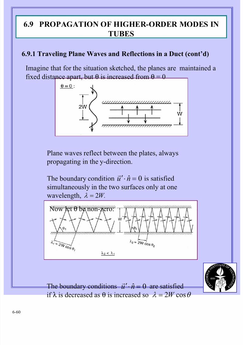
Imagine that for the situation sketched, the planes are maintained a
fixed distance apart, but θ is increased from θ = 0
Plane waves reflect between the plates, always
propagating in the y-direction.
The boundary condition is satisfiedsimultaneously in the two surfaces only at one
wavelength,
0ˆ =⋅′ nur
The boundary conditions are satisfied
if λ is decreased as θ is increased so
W.2=λ
θ λ cos2W =
Now let θ be non-zero:
0ˆ =⋅′ nur
6.9 PROPAGATION OF HIGHER-ORDER MODES IN
TUBES
6.9.1 Traveling Plane Waves and Reflections in a Duct (cont’d)
8/11/2019 Fundamentals of Acoustically Coupled Combustions
http://slidepdf.com/reader/full/fundamentals-of-acoustically-coupled-combustions 61/1206-61
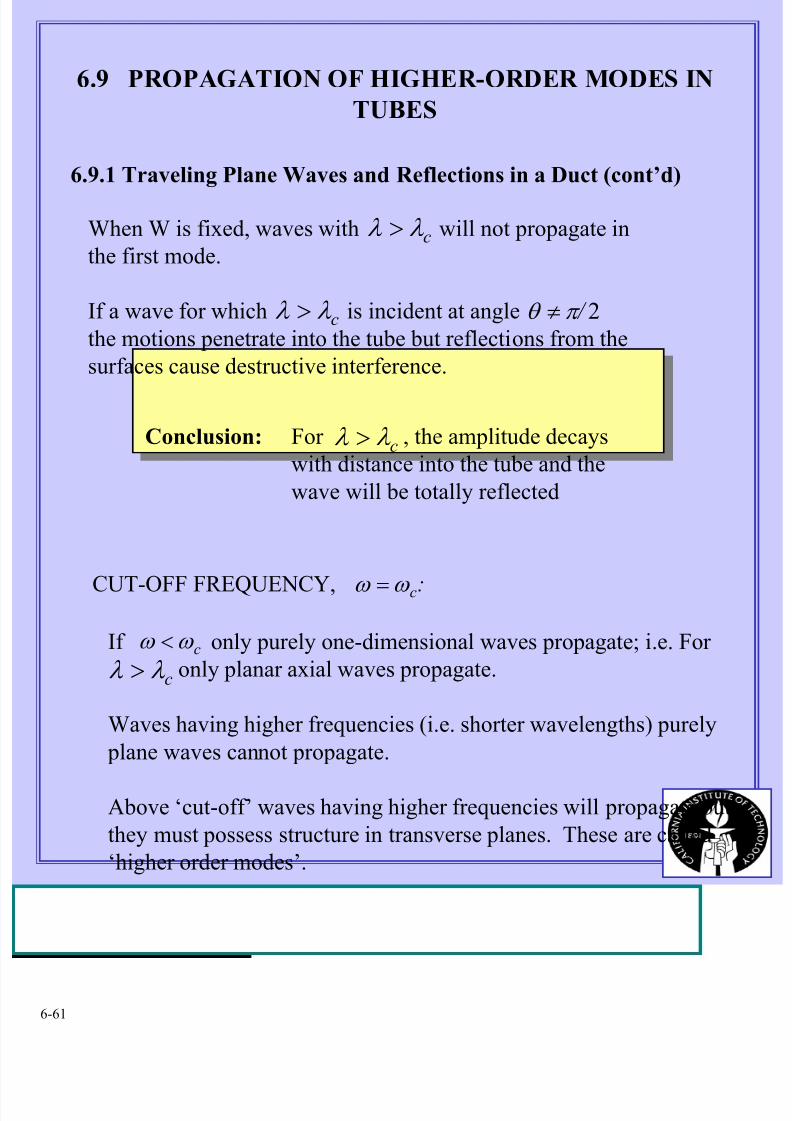
When W is fixed, waves with will not propagate in
the first mode.
If a wave for which is incident at angle
the motions penetrate into the tube but reflections from the
surfaces cause destructive interference.
cλ λ >
2 / π θ ≠
Conclusion: For , the amplitude decays
with distance into the tube and the
wave will be totally reflected
CUT-OFF FREQUENCY, :cω ω =
If only purely one-dimensional waves propagate; i.e. For
only planar axial waves propagate.
Waves having higher frequencies (i.e. shorter wavelengths) purely
plane waves cannot propagate.
Above ‘cut-off’ waves having higher frequencies will propagate but
they must possess structure in transverse planes. These are called
‘higher order modes’.
6.9 PROPAGATION OF HIGHER-ORDER MODES IN
TUBES
6.9.1 Traveling Plane Waves and Reflections in a Duct (cont’d)
cλ λ >
cλ λ >
cω ω <
cλ λ >
8/11/2019 Fundamentals of Acoustically Coupled Combustions
http://slidepdf.com/reader/full/fundamentals-of-acoustically-coupled-combustions 62/1206-62
6.9.2 Higher Order Modes as Solutions to the Wave Equation
in Three Dimensions
Solve for fixed:0ˆˆ 22 =+∇ pk p 0 /ak ω =
0ˆˆˆˆ 2
2
2
2
2
2
2
=+∂
∂+
∂
∂+
∂
∂ pk
z
p
y
p
x
p
Assume
( ) t it) z (k ie pe x,y P p z ω ω −−
==′ ˆ
for motion in a rectangular duct. The acoustic velocity is
∂
∂+
∂
∂+
∂
∂−=∇−= k
z
p j
y
pi
x
p pu ˆˆˆˆˆˆ1ˆ
1ˆ ρ ρ
r
Hence the boundary conditions on P(x,y) are
W , y y
P
V , x x
P
00
00
==∂
∂
==∂
∂
6.9 PROPAGATION OF HIGHER-ORDER MODES IN
TUBES
8/11/2019 Fundamentals of Acoustically Coupled Combustions
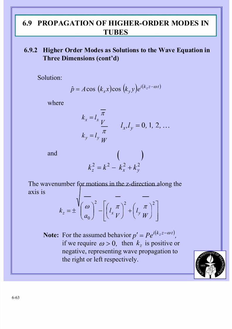
http://slidepdf.com/reader/full/fundamentals-of-acoustically-coupled-combustions 63/1206-63
Solution:
( ) ( ) ( )t z k i y x
z e yk xk A p ω −= coscosˆ
where
and
W l k
V l k
y y
x x
π
π
=
=K , , , ,l l y x 210=
2222
y x z k k k k +−=
The wavenumber for motions in the z-direction along the
axis is
+
−
±=
222
0 W l
V l
ak y x z
π π ω
Note: For the assumed behavior
if we require then is positive or
negative, representing wave propagation to
the right or left respectively.
( ) ,e P p t z k i z ω −=′
,0>ω z k
6.9 PROPAGATION OF HIGHER-ORDER MODES IN
TUBES
6.9.2 Higher Order Modes as Solutions to the Wave Equation in
Three Dimensions (cont’d)
8/11/2019 Fundamentals of Acoustically Coupled Combustions
http://slidepdf.com/reader/full/fundamentals-of-acoustically-coupled-combustions 64/1206-64
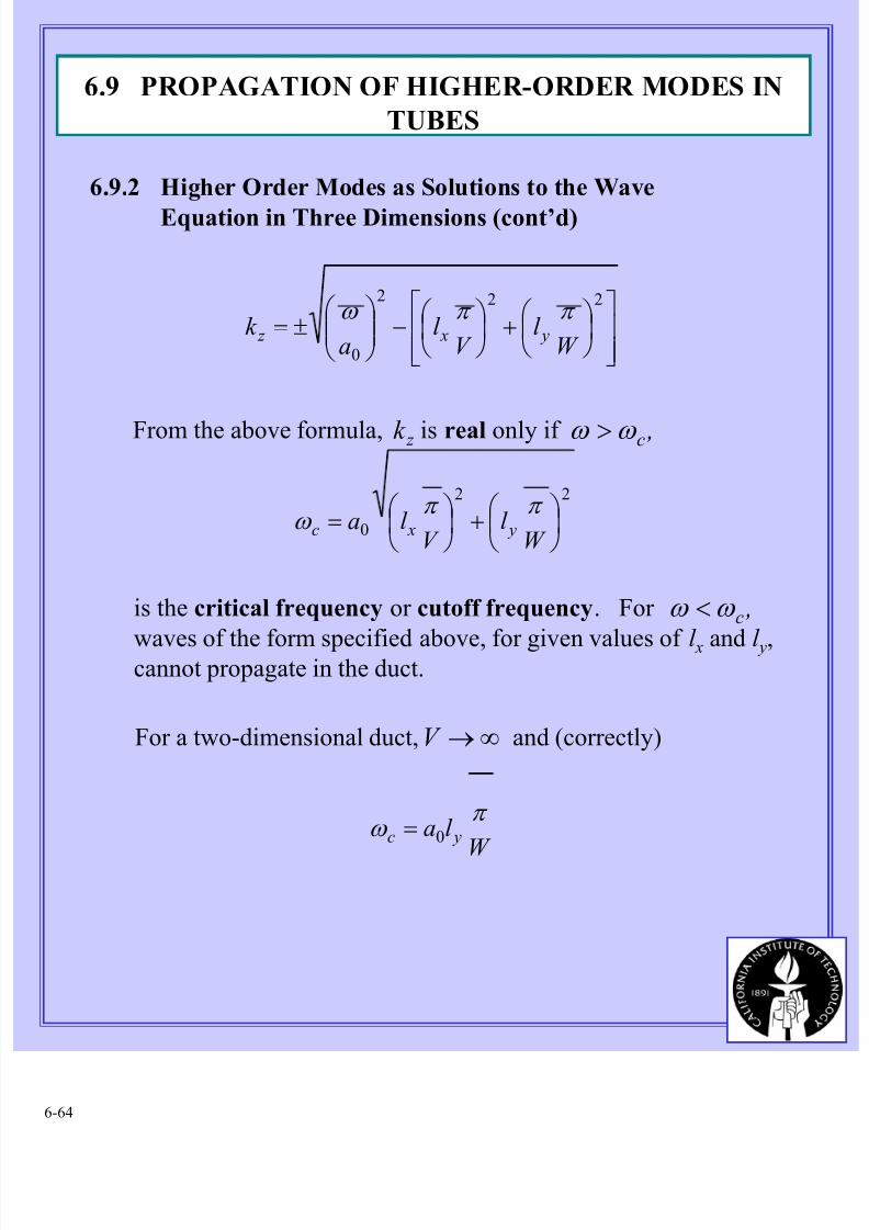
For a two-dimensional duct, and (correctly)
From the above formula, is real only if z k ,cω ω >
22
0
+
=
W l
V l a y xc
π π ω
is the critical frequency or cutoff frequency. For
waves of the form specified above, for given values of l x and l y,cannot propagate in the duct.
∞→V
W l a yc
π ω
0
=
+
−
±=
222
0 W l
V l
ak y x z
π π ω
,cω ω <
6.9 PROPAGATION OF HIGHER-ORDER MODES IN
TUBES
6.9.2 Higher Order Modes as Solutions to the Wave
Equation in Three Dimensions (cont’d)
8/11/2019 Fundamentals of Acoustically Coupled Combustions
http://slidepdf.com/reader/full/fundamentals-of-acoustically-coupled-combustions 65/1206-65
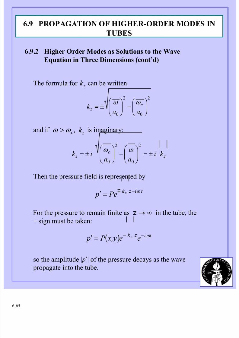
The formula for can be written
and if is imaginary:
t i z k z e P p ω −=′ m
,cω ω >
z k
z k
Then the pressure field is represented by
2
0
2
0
−
±=
aak c z
ω ω
z c
z k iaa
ik ±=
−
±=
2
0
2
0
ω ω
For the pressure to remain finite as in the tube, the
+ sign must be taken:
( ) t i z k ee x,y P p z ω −−=′
∞→z
so the amplitude | p′| of the pressure decays as the wave
propagate into the tube.
6.9 PROPAGATION OF HIGHER-ORDER MODES IN
TUBES
6.9.2 Higher Order Modes as Solutions to the Wave
Equation in Three Dimensions (cont’d)
8/11/2019 Fundamentals of Acoustically Coupled Combustions
http://slidepdf.com/reader/full/fundamentals-of-acoustically-coupled-combustions 66/1206-66
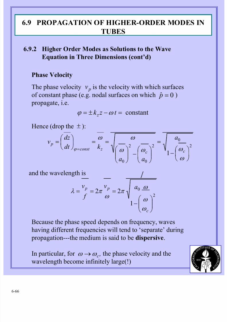
Phase Velocity
The phase velocity is the velocity with which surfaces
of constant phase (e.g. nodal surfaces on which )
propagate, i.e.
pv
constantt z k z =−±= ω ϕ
Hence (drop the ):±
2
0
2
0
2
0
1
−
=
−
==
=
=
ω
ω ω ω
ω ω
ϕ cc
z const p
a
aa
k dt
dz v
and the wavelength is
2
0
1
22
−
===
c
p p av
f
v
ω
ω
ω π
ω π λ
Because the phase speed depends on frequency, waveshaving different frequencies will tend to ‘separate’ during
propagation---the medium is said to be dispersive.
In particular, for the phase velocity and the
wavelength become infinitely large(!)
,cω ω →
0ˆ = p
6.9 PROPAGATION OF HIGHER-ORDER MODES IN
TUBES
6.9.2 Higher Order Modes as Solutions to the Wave
Equation in Three Dimensions (cont’d)
8/11/2019 Fundamentals of Acoustically Coupled Combustions
http://slidepdf.com/reader/full/fundamentals-of-acoustically-coupled-combustions 67/1206-67
Thus as and neither information nor
energy is carried down the duct for the mode in question.
Although the phase velocity is infinite, signals, information
and energy travel with finite speed, the group velocity.
Information (and hence net transfer of energy) occurs only
if the waves have nonuniformities, for example pulses.
The envelope of a pulse, or a ‘group’ of waves, travels with
speed , g v
,cω ω →
dk
d v g
ω =
[See good books on electromagnetic theory, or acoustics]
Here and
2
0
2
0
2
−
=
aak cω ω
2
0
2
0
2
0
202
0 1
−=
−
==
ω
ω ω ω
ω ω cc
g aaa
ak av
0→ g v
6.9 PROPAGATION OF HIGHER-ORDER MODES IN
TUBES
6.9.2 Higher Order Modes as Solutions to the Wave
Equation in Three Dimensions (cont’d)
8/11/2019 Fundamentals of Acoustically Coupled Combustions
http://slidepdf.com/reader/full/fundamentals-of-acoustically-coupled-combustions 68/1206-68
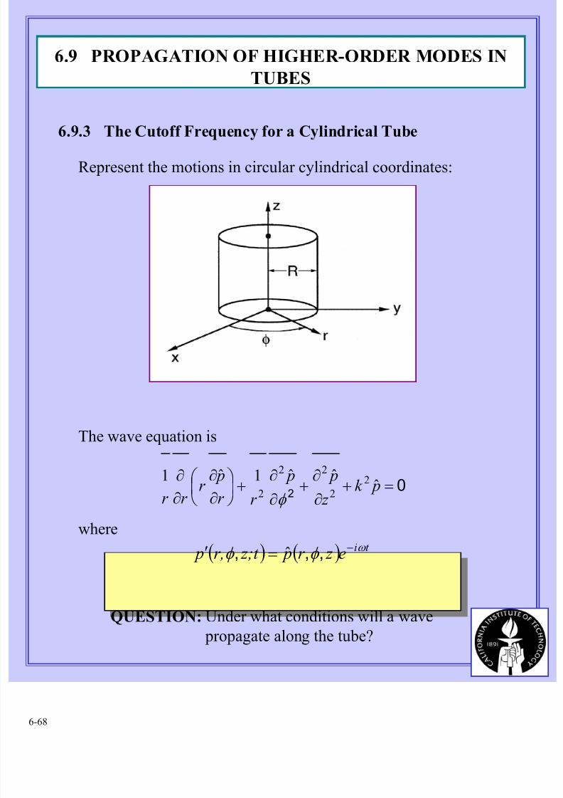
6.9.3 The Cutoff Frequency for a Cylindrical Tube
Represent the motions in circular cylindrical coordinates:
The wave equation is
where
02
=+∂
∂+
∂
∂+
∂
∂
∂
∂ pk
z
p p
r r
pr
r r ˆ
ˆˆ1ˆ1 2
2
22
2 φ
( ) ( ) t ie z r p z;t r, p ω φ φ −=′ ,,, ˆ
QUESTION: Under what conditions will a wave
propagate along the tube?
6.9 PROPAGATION OF HIGHER-ORDER MODES IN
TUBES
8/11/2019 Fundamentals of Acoustically Coupled Combustions
http://slidepdf.com/reader/full/fundamentals-of-acoustically-coupled-combustions 69/1206-69
( ) 011 22
2 =−+
∂
∂+
∂
∂
∂
∂ F k k
F
r r
F r
r r z 2
2
φ
Propagation along the tube is represented by the form
( ) ( ) ( )φ φ Φ= r Rr F ,
Substitution in the wave equation gives the equation
for F :
This equation is soluble by separation of variables:
Assume
( ) ( )t z k i z er, F p ω φ
−=′
and satisfyΦ R,
0md
d 2
2
2
=Φ+Φ
=
−−+
φ
01
2
222 R
r
mk k
dr
dRr
dr
d
r z
6.9 PROPAGATION OF HIGHER-ORDER MODES IN
TUBES
6.9.3 The Cutoff Frequency for a Cylindrical Tube (cont’d)
8/11/2019 Fundamentals of Acoustically Coupled Combustions
http://slidepdf.com/reader/full/fundamentals-of-acoustically-coupled-combustions 70/1206-70
( ) ( ) areand r Rφ ΦThe solutions for
K , , ,mm
m321
cos
sin=
=Φϕ
ϕ
( ) ( )r J r R mnm α =
with 222 z mn k k −=α
The values of are set by satisfying the boundarycondition on the pressure at the rigid lateral boundary:
mnα
0ˆ
=Φ=∂
∂ z ik z edr
dR
r
p
which ensures that the radial velocity vanishes on thewall. This condition requires
( )0=
= Rr
mnm
dr
r dJ α
6.9 PROPAGATION OF HIGHER-ORDER MODES IN
TUBES
6.9.3 The Cutoff Frequency for a Cylindrical Tube (cont’d)
8/11/2019 Fundamentals of Acoustically Coupled Combustions
http://slidepdf.com/reader/full/fundamentals-of-acoustically-coupled-combustions 71/1206-71
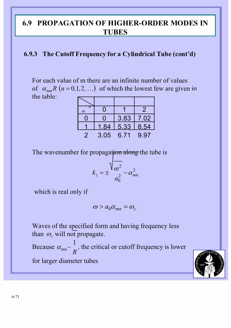
For each value of m there are an infinite number of values
of of which the lowest few are given in
the table:
( )K , , ,n Rmn 210=α
0 1 20 0 3.83 7.02
1 1.84 5.33 8.54
2 3.05 6.71 9.97
m
n
The wavenumber for propagation along the tube is
2
20
2
mn z a
k α ω −±=
which is real only if
cmna ω α ω => 0
Waves of the specified form and having frequency lessthan will not propagate.cω
Because the critical or cutoff frequency is lower
for larger diameter tubes
, R
~mn
1α
6.9 PROPAGATION OF HIGHER-ORDER MODES IN
TUBES
6.9.3 The Cutoff Frequency for a Cylindrical Tube (cont’d)
8/11/2019 Fundamentals of Acoustically Coupled Combustions
http://slidepdf.com/reader/full/fundamentals-of-acoustically-coupled-combustions 72/1206-72
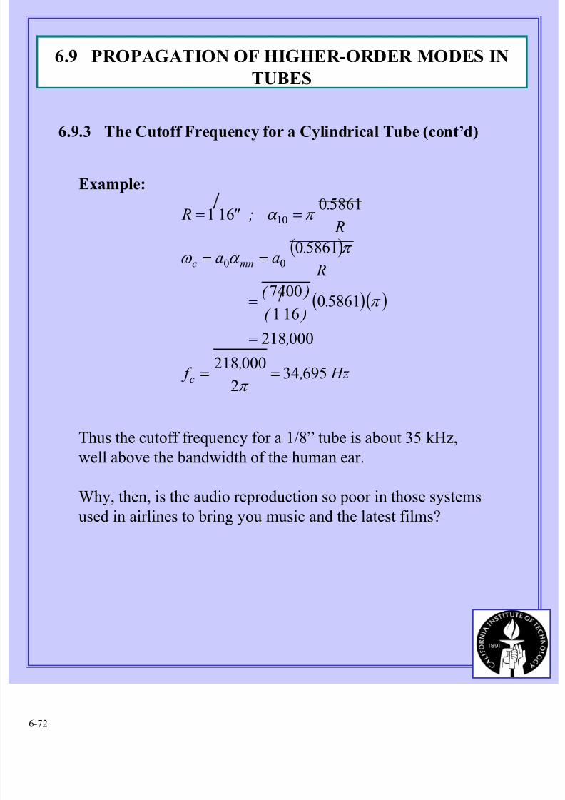
Example:
( )
( )( )
Hz , ,
f
,
. )(
)( R
.aa
R
.;" R
c
mnc
695342
000218
000218
58610161
7400
58610
58610161
00
10
==
=
=
==
==
π
π
π α ω
π α
Thus the cutoff frequency for a 1/8” tube is about 35 kHz,
well above the bandwidth of the human ear.
Why, then, is the audio reproduction so poor in those systems
used in airlines to bring you music and the latest films?
6.9 PROPAGATION OF HIGHER-ORDER MODES IN
TUBES
6.9.3 The Cutoff Frequency for a Cylindrical Tube (cont’d)
8/11/2019 Fundamentals of Acoustically Coupled Combustions
http://slidepdf.com/reader/full/fundamentals-of-acoustically-coupled-combustions 73/1206-73
6.10 NORMAL MODES: RESONANT FREQUENCIES
AND MODE SHAPES
DEFINITION: A normal mode of an oscillating system is amotion in which all parts of the system oscillate
sinusoidally at the same frequency, with fixed
relative phases and with amplitudes constant in
time.
6.10.1 An Elementary Example of Normal Modes: Two
Degrees of Freedom
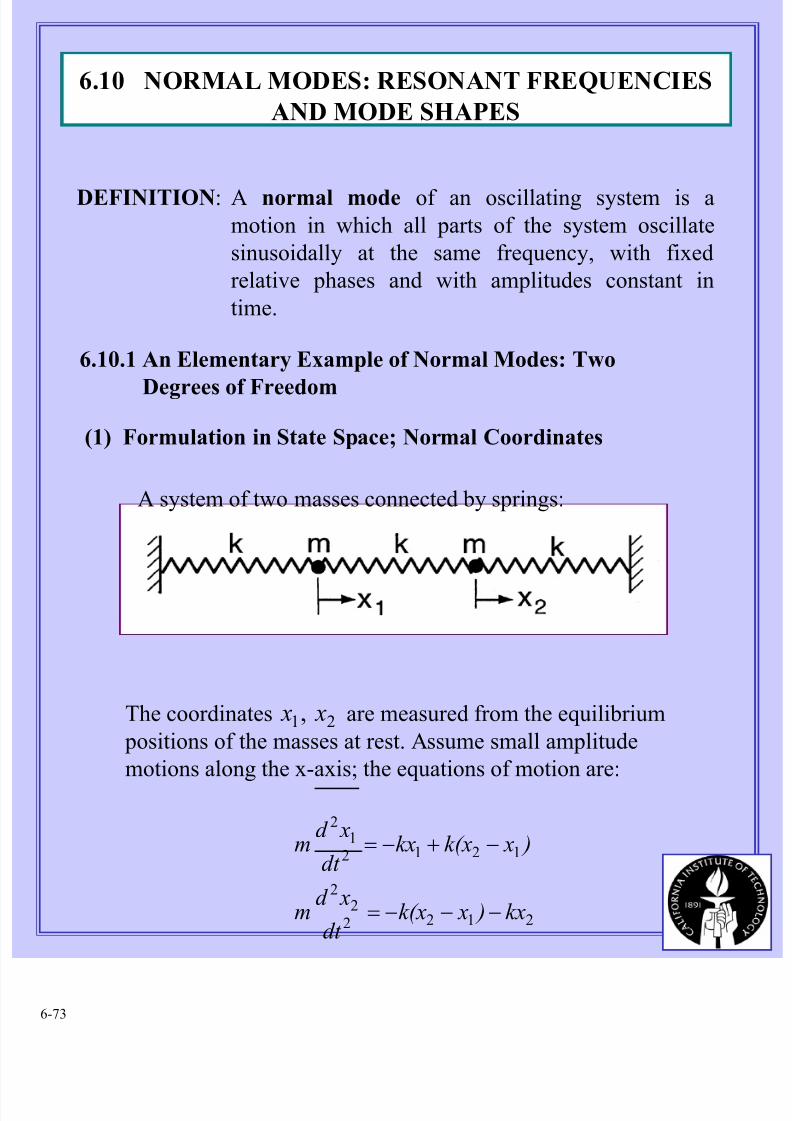
A system of two masses connected by springs:
The coordinates are measured from the equilibrium
positions of the masses at rest. Assume small amplitude
motions along the x-axis; the equations of motion are:
21, x x
21222
2
12121
2
kx ) xk(xdt
xd m
) xk(xkxdt
xd m
−−−=
−+−=
(1) Formulation in State Space; Normal Coordinates
8/11/2019 Fundamentals of Acoustically Coupled Combustions
http://slidepdf.com/reader/full/fundamentals-of-acoustically-coupled-combustions 74/120
8/11/2019 Fundamentals of Acoustically Coupled Combustions
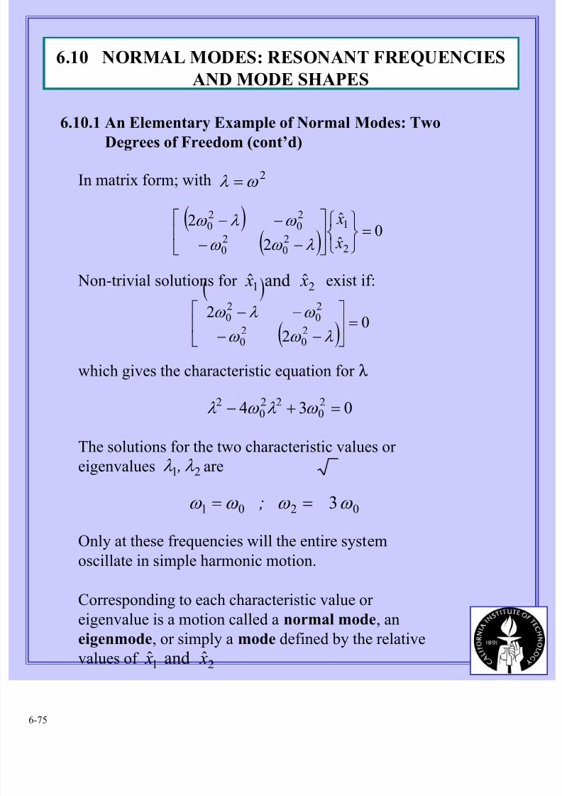
http://slidepdf.com/reader/full/fundamentals-of-acoustically-coupled-combustions 75/1206-75
Non-trivial solutions for exist if:21 ˆandˆ x x
( )0
2
220
20
20
20 =
−−
−−
λ ω ω
ω λ ω
In matrix form; with 2ω λ =
( )( )
0ˆ
ˆ
2
2
2
1
20
20
20
20 =
−−
−−
x
x
λ ω ω
ω λ ω
which gives the characteristic equation for λ
03420
220
2
=+− ω λ ω λ
The solutions for the two characteristic values or
eigenvalues are21 λ λ ,
0201 3ω ω ω ω == ;
Only at these frequencies will the entire systemoscillate in simple harmonic motion.
Corresponding to each characteristic value or
eigenvalue is a motion called a normal mode, an
eigenmode, or simply a mode defined by the relative
values of .21 ˆandˆ x x
6.10.1 An Elementary Example of Normal Modes: Two
Degrees of Freedom (cont’d)
6.10 NORMAL MODES: RESONANT FREQUENCIES
AND MODE SHAPES
8/11/2019 Fundamentals of Acoustically Coupled Combustions
http://slidepdf.com/reader/full/fundamentals-of-acoustically-coupled-combustions 76/1206-76
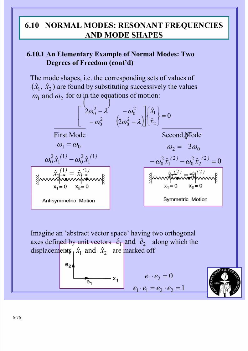
The mode shapes, i.e. the corresponding sets of values of
are found by substituting successively the values
for ω in the equations of motion:
( )0
ˆ
ˆ
2
2
2
1
2020
20
20 =
−−
−−
x
x
λ ω ω
ω λ ω
21 andω ω
)( i
)(
)( )(
x x
x x
112
11
20
11
20
01
ˆˆ
ˆˆ
=
−
=
ω ω
ω ω
)ˆ,ˆ( 21 x x
First Mode Second Mode
)( )(
)( )(
x x
x x
21
22
22
20
21
20
02
ˆˆ
0ˆˆ
3
=
=−−
=
ω ω
ω ω
Imagine an ‘abstract vector space’ having two orthogonal
axes defined by unit vectors along which thedisplacements are marked off
21 ˆandˆ ee21 ˆandˆ x x
1
0
2211
21
=⋅=⋅
=⋅
eeee
ee
6.10.1 An Elementary Example of Normal Modes: Two
Degrees of Freedom (cont’d)
6.10 NORMAL MODES: RESONANT FREQUENCIES
AND MODE SHAPES
8/11/2019 Fundamentals of Acoustically Coupled Combustions
http://slidepdf.com/reader/full/fundamentals-of-acoustically-coupled-combustions 77/1206-77
A motion of mass 1 in physical space is represented by
in this vector space and the normal modes can
be written11ˆ e
t ie x ω
( ) t i
t i )( )(
eee x
ee xe x X
1
1
211
21
211
11
ˆ
ˆˆ
ω
ω
+=
+=
( ) t i )(
t i )( )(
eee x
ee xe x X
2
2
212
1
22
212
12
ˆ
ˆˆ
ω
ω
m±=
+=
and the mode shapes are
( )2111ˆ ee += C X
where are normalization constant whose values
can be assigned according to some chosen rule; for example,
21, C C
e.g. 1)1( 21 == C C
211ˆ ee += X 212
ˆ ee +−= X
1ˆ2 =i X )(
( )2112
1eeE += ( )
2122
1eeE +−=
( ) 2
2211
222 because iii C C X =⋅+⋅= eeee
6.10.1 An Elementary Example of Normal Modes: Two
Degrees of Freedom (cont’d)
6.10 NORMAL MODES: RESONANT FREQUENCIES
AND MODE SHAPES
( )2122ˆ ee += C X
8/11/2019 Fundamentals of Acoustically Coupled Combustions
http://slidepdf.com/reader/full/fundamentals-of-acoustically-coupled-combustions 78/1206-78
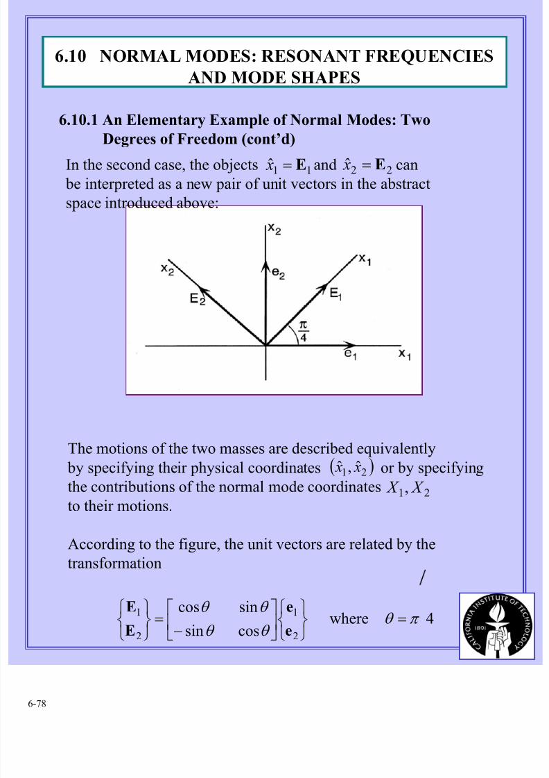
In the second case, the objects and can
be interpreted as a new pair of unit vectors in the abstract
space introduced above:
11ˆ E= x 22ˆ E= x
The motions of the two masses are described equivalently
by specifying their physical coordinates or by specifying
the contributions of the normal mode coordinates
to their motions.
According to the figure, the unit vectors are related by the
transformation
( )21 ˆ,ˆ x x
21, X X
4wherecossin
sincos
2
1
2
1π θ
θ θ
θ θ =
−=
e
e
E
E
6.10.1 An Elementary Example of Normal Modes: Two
Degrees of Freedom (cont’d)
6.10 NORMAL MODES: RESONANT FREQUENCIES
AND MODE SHAPES
8/11/2019 Fundamentals of Acoustically Coupled Combustions
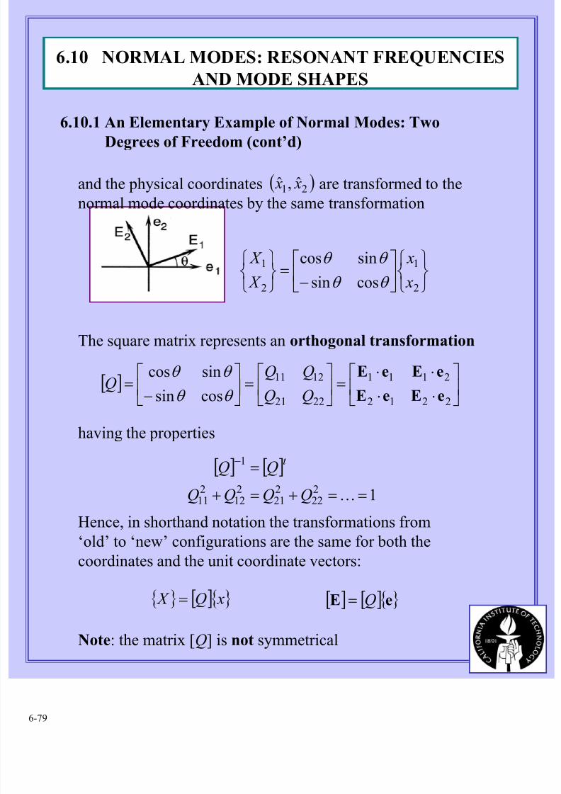
http://slidepdf.com/reader/full/fundamentals-of-acoustically-coupled-combustions 79/1206-79
and the physical coordinates are transformed to the
normal mode coordinates by the same transformation
( )21 ˆ,ˆ x x
−=
2
1
2
1
cossin
sincos
x
x
X
X
θ θ
θ θ
The square matrix represents an orthogonal transformation
[ ]
⋅⋅
⋅⋅=
=
−=
2212
2111
2221
1211
cossin
sincos
eEeE
eEeE
QQQ
θ θ
θ θ
having the properties
[ ] [ ]
1222
221
212
211
1
==+=+
=−
KQQQQ
QQ t
Hence, in shorthand notation the transformations from
‘old’ to ‘new’ configurations are the same for both thecoordinates and the unit coordinate vectors:
{ } [ ]{ } xQ X = [ ] [ ]{ }eE Q=
Note: the matrix [Q] is not symmetrical
6.10.1 An Elementary Example of Normal Modes: Two
Degrees of Freedom (cont’d)
6.10 NORMAL MODES: RESONANT FREQUENCIES
AND MODE SHAPES
8/11/2019 Fundamentals of Acoustically Coupled Combustions
http://slidepdf.com/reader/full/fundamentals-of-acoustically-coupled-combustions 80/1206-80
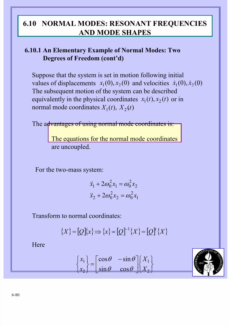
The equations for the normal mode coordinates
are uncoupled.
Suppose that the system is set in motion following initial
values of displacements and velocities .
The subsequent motion of the system can be described
equivalently in the physical coordinates or in
normal mode coordinates .
)0(),0( 21 x x )0(),0( 21 x x &&
)(),( 21 t xt x
)(),(21
t X t X
The advantages of using normal mode coordinates is:
For the two-mass system:
1202
202
2201
201
2
2
x x x
x x x
ω ω
ω ω
=+
=+
&&
&&
Transform to normal coordinates:
{ } [ ]{ } { } [ ] { } [ ] { } X Q X Q x xQ X t ==⇒= −1
Here
−=
2
1
2
1
cossin
sincos
X
X
x
x
θ θ
θ θ
6.10.1 An Elementary Example of Normal Modes: Two
Degrees of Freedom (cont’d)
6.10 NORMAL MODES: RESONANT FREQUENCIES
AND MODE SHAPES
8/11/2019 Fundamentals of Acoustically Coupled Combustions
http://slidepdf.com/reader/full/fundamentals-of-acoustically-coupled-combustions 81/1206-81
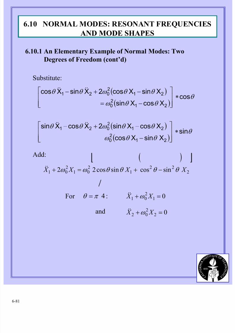
Substitute:
( )
( )
( )
( ) θ
θ θ ω
θ θ ω θ θ
θ θ θ ω
θ θ ω θ θ
sinXsinXcos
XcosXsin2XcosXsin
cosXcosXsin
XsinXcos2XsinXcos
2120
212021
2120
212021
∗
−
−+−
∗
−=
−+−
&&&&
&&&&
Add:
:4π θ = 01201 =+ X X ω &&
02202 =+ X X ω &&and
2
22
1
2
01
2
01 sincossincos22 X X X X θ θ θ θ ω ω −+=+&&
For
6.10.1 An Elementary Example of Normal Modes: Two
Degrees of Freedom (cont’d)
6.10 NORMAL MODES: RESONANT FREQUENCIES
AND MODE SHAPES
8/11/2019 Fundamentals of Acoustically Coupled Combustions
http://slidepdf.com/reader/full/fundamentals-of-acoustically-coupled-combustions 82/1206-82
Solutions for :
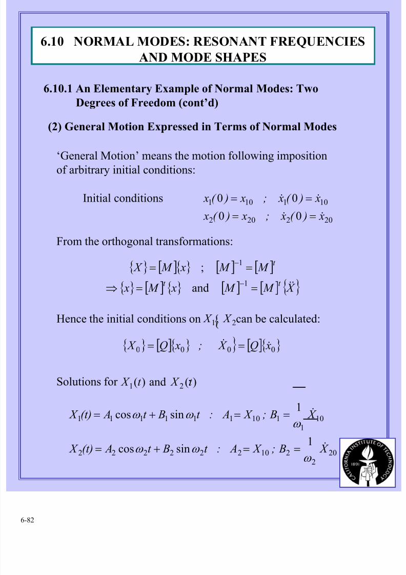
(2) General Motion Expressed in Terms of Normal Modes
‘General Motion’ means the motion following imposition
of arbitrary initial conditions:
Initial conditions
202202
101101
00
00
x )( x; x )( x
x )( x; x )( x
&&&&
====
From the orthogonal transformations:
{ } [ ]{ } [ ] [ ]
{ } [ ] { } [ ] [ ] { } X M M x M x
M M x M X
t t
t
&&==⇒
==−
−
1
1
and
;
Hence the initial conditions on can be calculated:21, X X
{ } [ ]{ } } [ ]{ }0000 xQ X ; xQ X && ==
)(and)( 21 t X t X
202
210222222
101
110111111
1sincos
1sincos
X B; X A:t Bt A(t) X
X B; X A:t Bt A(t) X
&
&
ω ω ω
ω ω ω
==+=
==+=
6.10.1 An Elementary Example of Normal Modes: Two
Degrees of Freedom (cont’d)
6.10 NORMAL MODES: RESONANT FREQUENCIES
AND MODE SHAPES
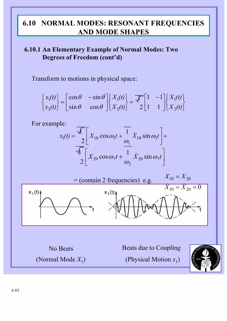
8/11/2019 Fundamentals of Acoustically Coupled Combustions
http://slidepdf.com/reader/full/fundamentals-of-acoustically-coupled-combustions 83/1206-83
Transform to motions in physical space:
−=
−=
(t) X
(t) X
(t) X
(t) X
(t) x
(t) x
2
1
2
1
2
1
11
11
2
1
cossin
sincos
θ θ
θ θ
For example:
+
+
+=
t X t X
t X t X (t) x
220
2
220
1101
1101
sin1
cos
2
1
sin1
cos2
1
ω
ω
ω
ω ω
ω
&
&
No Beats Beats due to Coupling
(Normal Mode X 1) (Physical Motion x1)
= (contain 2 frequencies) e.g.02010
2010
==
=
X X
X X
&&
6.10.1 An Elementary Example of Normal Modes: Two
Degrees of Freedom (cont’d)
6.10 NORMAL MODES: RESONANT FREQUENCIES
AND MODE SHAPES
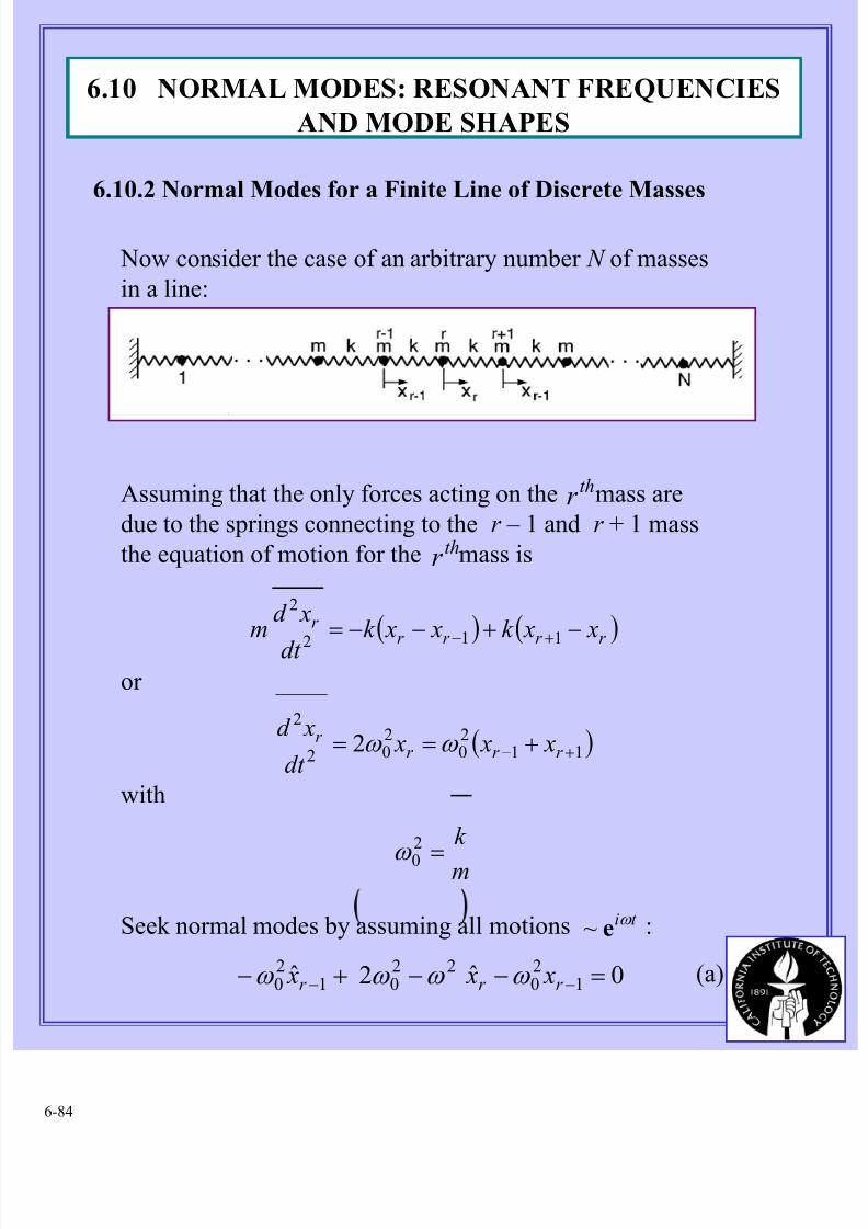
8/11/2019 Fundamentals of Acoustically Coupled Combustions
http://slidepdf.com/reader/full/fundamentals-of-acoustically-coupled-combustions 84/1206-84
6.10.2 Normal Modes for a Finite Line of Discrete Masses
Now consider the case of an arbitrary number N of masses
in a line:
Assuming that the only forces acting on the mass are
due to the springs connecting to the r – 1 and r + 1 mass
the equation of motion for the mass is
thr
thr
( ) ( )r r r r r
x xk x xk dt
xd m −+−−= +− 112
2
or
( )1120
202
2
2 +− +== r r r r x x x
dt
xd ω ω
with
mk =2
0ω
Seek normal modes by assuming all motions :t iω e~
0ˆ2ˆ 120
2201
20 =−−+− −− r r r x x x ω ω ω ω (a)
6.10 NORMAL MODES: RESONANT FREQUENCIES
AND MODE SHAPES
8/11/2019 Fundamentals of Acoustically Coupled Combustions
http://slidepdf.com/reader/full/fundamentals-of-acoustically-coupled-combustions 85/1206-85
6.10.2 Normal Modes for a Finite Line of Discrete Masses
The set of equations can be written
[ ] [ ] { } 0ˆ2 =− x I V ω
(1) Non-trivial solutions exist only if ω2 takes on
characteristic or eigen values, the roots of the secular
or characteristic equation
02 =− ijijV δ ω
N masses, N equations, N positive roots
N ω ω ω K,, 21
In matrix form:
( )
( )
( )
0
ˆ
ˆ
ˆ
ˆ
200
0
0020
02
0002
3
2
1
220
20
20
20
20
220
20
20
220
20
20
220
=
−−
−
−−−−
−−−
−−
N x
x
x
x
M
LL
M
OMM
ML
L
ω ω ω
ω
ω ω ω ω ω
ω ω ω ω
ω ω ω
6.10 NORMAL MODES: RESONANT FREQUENCIES
AND MODE SHAPES
8/11/2019 Fundamentals of Acoustically Coupled Combustions
http://slidepdf.com/reader/full/fundamentals-of-acoustically-coupled-combustions 86/1206-86
6.10.2 Normal Modes for a Finite Line of Discrete Masses
(cont’d)
(2) For every value of there is a corresponding
set of found as solutions to equations (a):
2ω
i x
S iS x2 ↔ω
The are the components of the normal mode
vector in physical coordinates, i.e. in the normalmode s,
si x th s
t iS i
S i
S e x x ω ˆ=
and is the amplitude of motion of the mass
in the mode.
S i x
th s
thi
(3) For each modal vector there is a multiplicative constant whose value can be set by some
normalization rule, e.g.
S i x
( ) ( ) ( ) 1ˆˆˆ22
2
2
1 =+++ S N
S S x x x K
Hence the can be interpreted as the
components of a unit eigenvector in the abstract
vector space spanned by the Cartesian unit vectors
lying along the axes
S N
S S x x x ˆˆ,ˆ 21 K sE
{ } N eee K,, 21 { } N x x x ˆ,ˆ,ˆ 21 K
6.10 NORMAL MODES: RESONANT FREQUENCIES
AND MODE SHAPES
8/11/2019 Fundamentals of Acoustically Coupled Combustions
http://slidepdf.com/reader/full/fundamentals-of-acoustically-coupled-combustions 87/1206-87
(4) Transformation to normal coordinates is accomplished
with the ‘modal matrix’ of the transformation. Let the
be unit vectors obtained by rotating the
system according to the rule N X X X ˆ,ˆ,ˆ
21 K
{ } N x x x ˆ,ˆ,ˆ 21 K
=
N N N N N
N
N
N x
x x
x x x
x x x x x x
X
X X
ˆ
ˆˆ
ˆˆˆ
ˆˆˆˆˆˆ
ˆ
ˆ
ˆ
2
1
21
222
22
11
2
1
1
2
1
M
L
LM
LL
M
The elements of the columns are the components of the
eigenvectors; i.e.
=
N N N N N
N
N x
x
x
X
X
X
ˆ
ˆ
ˆ
ˆ
ˆ
ˆ
2
1
21
22
12
112
11
2
1
M
L
LM
ML
L
M
EEE
EE
EEE
or and{ } [ ] X M x ˆˆ = { } [ ] { } [ ] { } x M x M X t
ˆˆˆ 1 == −
[ M ] = modal matrix
[ ] [ ]t M M =−1so [ M ] is orthogonal (not proved here)
6.10 NORMAL MODES: RESONANT FREQUENCIES
AND MODE SHAPES
6.10.2 Normal Modes for a Finite Line of Discrete Masses
(cont’d)
8/11/2019 Fundamentals of Acoustically Coupled Combustions
http://slidepdf.com/reader/full/fundamentals-of-acoustically-coupled-combustions 88/1206-88
(5) In the normal coordinates, transformed is
diagonal
[ ]V
[ ]{ } { } [ ][ ] [ ]
[ ] [ ][ ]
=
=⇒=
−
O
O
O
O
21
22
S
S S
S S
M V M
M M V E E V
ω
ω ω
[ ]
=
|
| N
|
|
|
|
E E E M K21
(6) The equations for the normal coordinates X (t )
are uncoupled
Equations for physical coordinates { } [ ]{ } xV x =&&
[ ]{ } [ ][ ] { } x M V x M =&&Transform
{ } [ ] [ ][ ] { }
{ } { } X X
X M V M X
S
=
= −
O
O
&&
&&
2
1
ω
Result: Transformation to normal or modal coordinates
diagonalizes the potential energy matrix and the
equations of motion for the modal coordinates
are uncoupled.
6.10 NORMAL MODES: RESONANT FREQUENCIES
AND MODE SHAPES
6.10.2 Normal Modes for a Finite Line of Discrete Masses
(cont’d)
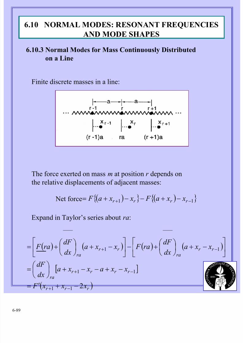
8/11/2019 Fundamentals of Acoustically Coupled Combustions
http://slidepdf.com/reader/full/fundamentals-of-acoustically-coupled-combustions 89/1206-89
6.10.3 Normal Modes for Mass Continuously Distributed
on a Line
Finite discrete masses in a line:
The force exerted on mass m at position r depends onthe relative displacements of adjacent masses:
( ){ } ( ){ }11 −+ −+−−+= r r r r x xa F x xa F Net force
Expand in Taylor’s series about ra:
( ) ( ) ( ) ( )
[ ]
( )r r r
r r r r ra
r r ra
r r ra
x x x F
x xa x xadx
dF
x xadx
dF ra F x xa
dx
dF ra F
211
11
11
−+′=
−+−−+
=
−+
+−
−+
+=
−+
−+
−+
6.10 NORMAL MODES: RESONANT FREQUENCIES
AND MODE SHAPES
8/11/2019 Fundamentals of Acoustically Coupled Combustions
http://slidepdf.com/reader/full/fundamentals-of-acoustically-coupled-combustions 90/1206-90
6.10.3 Normal Modes for Mass Continuously Distributed
on a Line (cont’d)
Equation of motion for r th mass:
( ) ( )[ ]
0
),(;
=
−−
−−
=≈
=′
=′=−−−′−
−+
=
=−+
a
x x
a
x x
aT x
a
m
pT F a
F
dx
dF F
dx
dF F x x x x F xm
r r r r r
x
xr r r r r
11
0
0
00110
1
ilitycompressibor tension
0
&&
&&
γ δ δ
Take limit finite linear density ρ =→→a
mma but0,0
2
2
11
1
11
z
x
z
x
z
x
a
a
x
a
x
aa
x x
a
x x
a
r r
r r
r r r r
∂
∂→
∂
∂−
∂
∂→
−
→
−−
−
−+
−+
−+ δ δ
In the limit:
0)( 2
2
2
2
=∂∂−∂∂ z xT
t x z ρ
02
22
2
2
=∂
∂−
∂
∂
z
xa
t
x,2
ρ
T a = wave propagation
speed
z : coordinate along the line (string or column of a fluid)
6.10 NORMAL MODES: RESONANT FREQUENCIES
AND MODE SHAPES
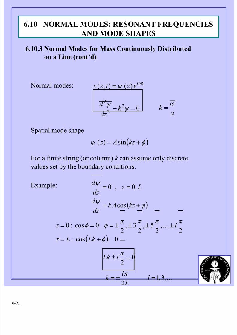
8/11/2019 Fundamentals of Acoustically Coupled Combustions
http://slidepdf.com/reader/full/fundamentals-of-acoustically-coupled-combustions 91/1206-91
6.10.3 Normal Modes for Mass Continuously Distributed
on a Line (cont’d)
Normal modes: t ie z t z x ω ψ )(),( =
02
2
2
=+ ψ ψ
k
dz
d
a
k ω =
Spatial mode shape
( )φ ψ += kz A z sin)(
For a finite string (or column) k can assume only discrete
values set by the boundary conditions.
( )φ ψ
ψ
+=
==
kz Ak dz
d
L z dz
d
cos
,0,0
( ) 0cos:2
,2
5,2
3,2
0cos:0
=+=
±±±±===
φ
π π π π φ φ
Lk L z
l z K
02
=± π l Lk
L
l k
2
π ±= K,3,1=l
Example:
6.10 NORMAL MODES: RESONANT FREQUENCIES
AND MODE SHAPES
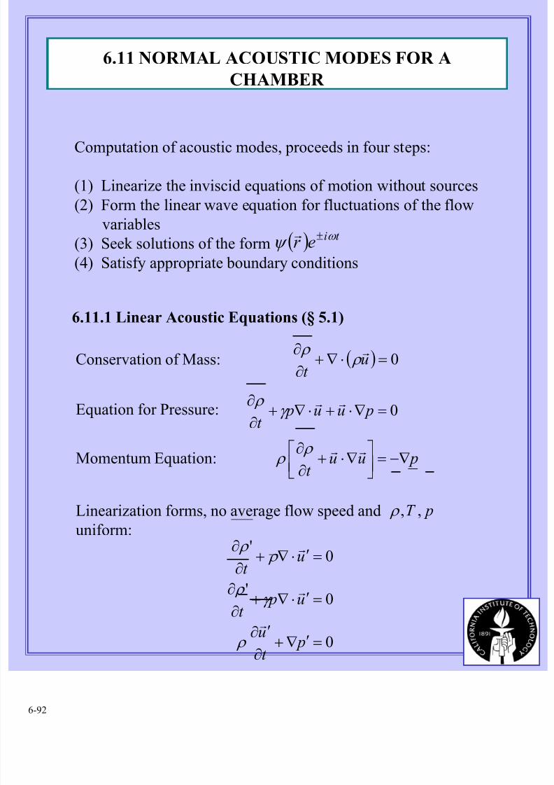
8/11/2019 Fundamentals of Acoustically Coupled Combustions
http://slidepdf.com/reader/full/fundamentals-of-acoustically-coupled-combustions 92/1206-92
6.11 NORMAL ACOUSTIC MODES FOR A
CHAMBER
Computation of acoustic modes, proceeds in four steps:
(1) Linearize the inviscid equations of motion without sources
(2) Form the linear wave equation for fluctuations of the flow
variables
(3) Seek solutions of the form
(4) Satisfy appropriate boundary conditions
( ) t ier ω ψ ±r
6.11.1 Linear Acoustic Equations (§ 5.1)
Conservation of Mass:
Equation for Pressure:
Momentum Equation:
Linearization forms, no average flow speed and
uniform:
pT ,, ρ
( ) 0=⋅∇+∂
∂u
t
r ρ
ρ
0=∇⋅+⋅∇+∂∂ puu p
t rrγ ρ
puut
−∇=
∇⋅+
∂
∂ rr ρ ρ
0
0'
0'
=′∇+∂
′∂
=′⋅∇+∂
∂
=′⋅∇+∂
∂
pt
u
u pt
ut
r
r
r
ρ
γ ρ
ρ ρ
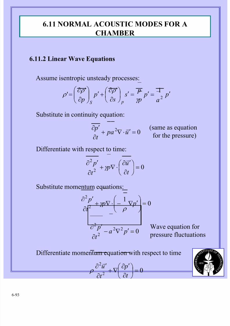
8/11/2019 Fundamentals of Acoustically Coupled Combustions
http://slidepdf.com/reader/full/fundamentals-of-acoustically-coupled-combustions 93/1206-93
6.11.2 Linear Wave Equations
02 =′⋅∇+∂
′∂ua p
t
p r
02
2
=
∂
′∂
⋅∇+∂
′∂
t
u pt
p r
γ
Assume isentropic unsteady processes:
pa
p p
p s
s p
p pS
′=′=′
∂
∂+′
∂
∂=
2
1'''
γ
ρ ρ ρ
Substitute in continuity equation:
(same as equation
for the pressure)
Differentiate with respect to time:
Substitute momentum equations:
01
2
2
=
′∇−⋅∇+
∂
′∂ p p
t
p
ρ γ
022
2
2
=′∇−∂
′∂ pa
t
p Wave equation for
pressure fluctuations
Differentiate momentum equation with respect to time
02
2
=
∂
′∂∇+
∂
′∂
t
p
t
ur
ρ
6.11 NORMAL ACOUSTIC MODES FOR A
CHAMBER
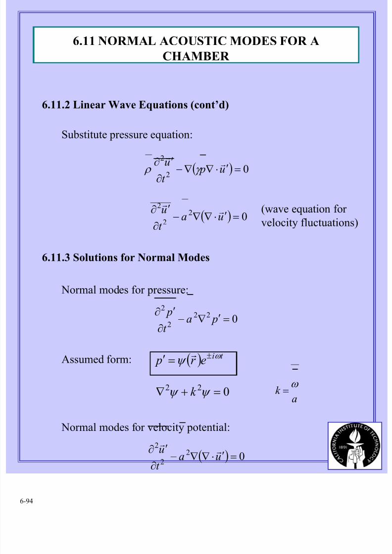
8/11/2019 Fundamentals of Acoustically Coupled Combustions
http://slidepdf.com/reader/full/fundamentals-of-acoustically-coupled-combustions 94/120
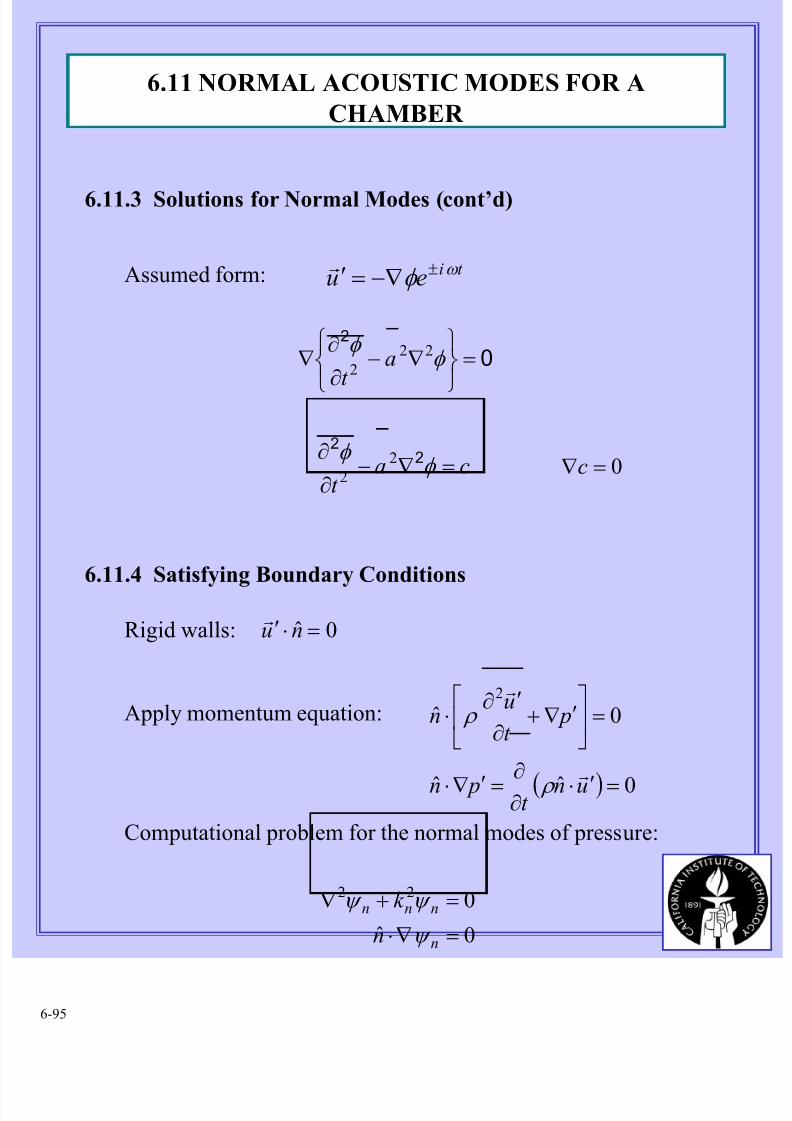
8/11/2019 Fundamentals of Acoustically Coupled Combustions
http://slidepdf.com/reader/full/fundamentals-of-acoustically-coupled-combustions 95/1206-95
6.11.3 Solutions for Normal Modes (cont’d)
02
=
∇−
∂
∂∇ φ
φ 22
2 a
t
Assumed form: t ieu ω φ ±−∇=′r
cat
=∇−∂
∂φ
φ 22
2
20=∇c
6.11.4 Satisfying Boundary Conditions
Rigid walls:
Apply momentum equation:
Computational problem for the normal modes of pressure:
0ˆ =⋅′ nur
( ) 0ˆˆ
0ˆ2
=′⋅∂∂=′∇⋅
=
′∇+
∂
′∂⋅
unt
pn
pt
un
r
r
ρ
ρ
0ˆ
022
=∇⋅
=+∇
n
nnn
n
k
ψ
ψ ψ
6.11 NORMAL ACOUSTIC MODES FOR A
CHAMBER
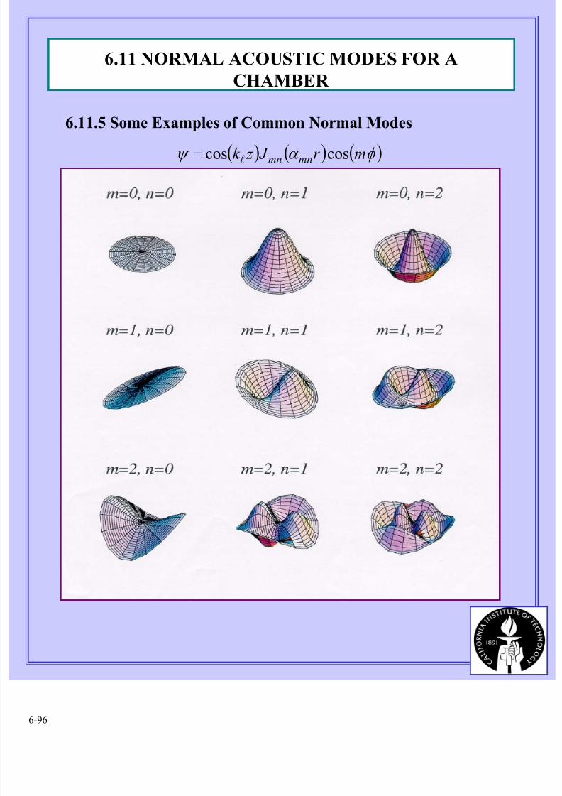
8/11/2019 Fundamentals of Acoustically Coupled Combustions
http://slidepdf.com/reader/full/fundamentals-of-acoustically-coupled-combustions 96/1206-96
6.11.5 Some Examples of Common Normal Modes
( ) ( ) ( )φ α ψ mr J z k mnmn coscos l=
6.11 NORMAL ACOUSTIC MODES FOR A
CHAMBER
8/11/2019 Fundamentals of Acoustically Coupled Combustions
http://slidepdf.com/reader/full/fundamentals-of-acoustically-coupled-combustions 97/1206-97
heat release
presence of mean flow
condensed material suspended in the gas
conversion of condensed material to gas
motion of the boundary
6.12 A METHOD OF SPATIAL AVERAGING FOR
SOLVING INTERNAL ACOUSTIC PROBLEMS WITH
SOURCES
Many possible kinds of sources of acoustic waves exist; e.g.:
M
Here assume time-varying heat sources distributed in the
volume, and distributed motions of the boundary
The equation for the pressure with heat sources (§ 4.5 )
QC
R puu p
t
p
V
&rr=∇⋅+⋅∇+
∂
∂γ
Boundary condition for a moving boundary
∇⋅+
∂
∂⋅−=∇⋅ uu
t
un pn
rrr
r ρ ρ ˆˆ
Linearized forms:
t
un pn
pt
u
QC
Ru p
t
p
V
∂
′∂
⋅−=′∇⋅
=′∇+∂
′∂
′=′⋅∇+∂
′∂
r
r
&r
ˆˆ
0
ρ
ρ
γ
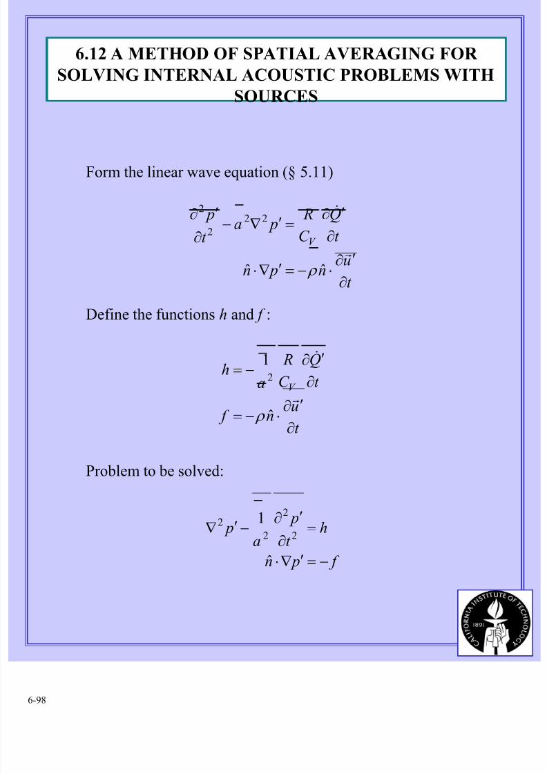
8/11/2019 Fundamentals of Acoustically Coupled Combustions
http://slidepdf.com/reader/full/fundamentals-of-acoustically-coupled-combustions 98/1206-98
t un pn
t
Q
C
R pa
t
p
V
∂ ′∂⋅−=′∇⋅
∂
′∂=′∇−
∂
′∂
r
&
ˆˆ
22
2
2
ρ
Form the linear wave equation (§ 5.11)
Define the functions h and f :
t
un f
t
Q
C
R
ah
V
∂′∂⋅−=
∂
′∂−=
r
&
ˆ
12
ρ
f pn
ht
p
a p
−=′∇⋅
=∂
′∂
−′∇
ˆ
12
2
2
2
Problem to be solved:
6.12 A METHOD OF SPATIAL AVERAGING FOR
SOLVING INTERNAL ACOUSTIC PROBLEMS WITH
SOURCES
8/11/2019 Fundamentals of Acoustically Coupled Combustions
http://slidepdf.com/reader/full/fundamentals-of-acoustically-coupled-combustions 99/1206-99
(1) If h, f are small, then should not differ
greatly from its form given by a solution to the
homogeneous problem
(2) Hence ‘subtract’ the two problems and devise
a scheme for calculating the difference, due to
non-zero values of h, f .
(3) Any solution to the homogeneous problem can
be expressed as a superposition of normal
acoustic modes:
6.12.1 Oscillator Equations for Unsteady Motions in a
Chamber
0ˆ
01
2
2
2
2
=′∇⋅
=∂
′∂−′∇
h
hh
pn
t
p
a p
Assume h, f ‘small’ perturbations and given
The idea:
(i) is in general complex but independent of t .
(ii) Each term in the series, and therefore the
sum, i.e. is an exact solution to the
homogeneous problem.
nC
( ) ,t ,r ph
r
( ) ( ) t innh
ner C t ,r p ω ψ rr
∑=′
Notes:
p′
6.12 A METHOD OF SPATIAL AVERAGING FOR
SOLVING INTERNAL ACOUSTIC PROBLEMS WITH
SOURCES
8/11/2019 Fundamentals of Acoustically Coupled Combustions
http://slidepdf.com/reader/full/fundamentals-of-acoustically-coupled-combustions 100/1206-100
6.12.1 Oscillator Equations for Unsteady Motions in a
Chamber (cont’d)
(4) The solution when sources are present will not differ greatly
from a normal mode or a combination of normal modes.
Hence, compare the perturbed (actual) solution p′ with one
of the normal modes .
(5) Formal Procedure:
(i) Multiply (1) by , (2) by p′, and subtract
(ii) Integrate over the volume of the chamber
(iii) Rewrite the first integral by using Green’s theorem and
substitute the boundary conditions (3) and (4):
nψ
(1) (2)
(3) (4)
ht
p
a p =
∂
′∂−′∇
2
2
2
2 1022 =+∇ nnn k ψ ψ
nψ
( ) h pk t
p
a p p nnnnnn ψ ψ ψ ψ ψ =
′+
∂
′∂−∇′−′∇ 2
2
2
2
22 1
[ ]∫ ∫∫ =
′+
∂
′∂−∇′−′∇ dV hdV pk
t
p
adV p p nnn
nnn ψ ψ
ψ ψ ψ 2
2
2
2
22
f pn −=′∇⋅ 2ˆ 0ˆ =∇⋅ nn ψ
6.12 A METHOD OF SPATIAL AVERAGING FOR
SOLVING INTERNAL ACOUSTIC PROBLEMS
WITH SOURCES
[ ]
∫∫
∫∫∫
−=
⋅∇−⋅∇=∇−∇
dS f
dS n pn pdV p p
n
nnnn
ψ
ψ ψ ψ ψ 321
0
22 ˆ'ˆ'''
8/11/2019 Fundamentals of Acoustically Coupled Combustions
http://slidepdf.com/reader/full/fundamentals-of-acoustically-coupled-combustions 101/1206-101
6.12.1 Oscillator Equations for Unsteady Motions in a Chamber (cont’d)
{ }∫ ∫∫∫∫ +−=′+
∂
′∂dS f dV hadV pdV
t
p
nnnnn ψ ψ ψ ω ψ 22
2
2
The equation in (ii) becomes
Note: This equation is the spatial average of the
difference between the perturbed and unperturbed
problems with an acoustics mode
as weighting function.
(iv) Now expand as a synthesis of basis functions,
selected here to be the unperturbed acoustic modes with
time-dependent amplitudes:
( )t r p ,r
′
( ) ( ) ( )r t pt r p mm
m
rrψ η ∑
∞
=
=′1
,
(∗)
(∗∗)
6.12 A METHOD OF SPATIAL AVERAGING FOR
SOLVING INTERNAL ACOUSTIC PROBLEMS
WITH SOURCES
8/11/2019 Fundamentals of Acoustically Coupled Combustions
http://slidepdf.com/reader/full/fundamentals-of-acoustically-coupled-combustions 102/1206-102
6.12.1 Oscillator Equations for Unsteady Motions in a
Chamber (cont’d)
Substitute (∗∗) in (∗):
( ) ( ) ( ) ( )
{ }
( ) ( ) ( ) ( )
{ }∫∫
∑∑
∫∫
∑∑
+∫−=
∫+∫
+∫−=
∫+∫
∞∞
∞∞
dS f dV ha
dV r r (t) pdV r r p
dS f dV ha
dV r r (t) pdV r r p
mm
mmmnmmm
mm
mmmnmmm
ψ ψ
ψ ψ η ω ψ ψ η
ψ ψ
ψ ψ η ω ψ ψ η
2
1
2
1
2
1
2
1
rrrr&&
rrrr&&
Orthogonality: ( ) ( ) mnmmm E dV r r δ ψ ψ 2=∫ rr
{ }∫∫+∫−=+ dS f dV h E p
a
dt
d nn
n
nnn ψ ψ η ω
η 2
22
2
2
Oscillator Equations
6.12 A METHOD OF SPATIAL AVERAGING FOR
SOLVING INTERNAL ACOUSTIC PROBLEMS WITH
SOURCES
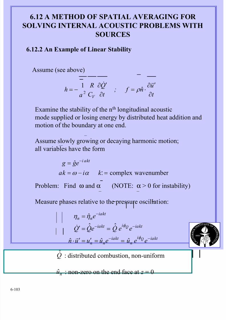
8/11/2019 Fundamentals of Acoustically Coupled Combustions
http://slidepdf.com/reader/full/fundamentals-of-acoustically-coupled-combustions 103/1206-103
Problem: Find ω and α (NOTE: α > 0 for instability)
6.12.2 An Example of Linear Stability
Assume (see above)
t
un f ;
t
Q
C
R
ah
V ∂
′∂⋅=
∂
′∂−=
r&ˆ
12
ρ
Examine the stability of the nth longitudinal acousticmode supplied or losing energy by distributed heat addition and
motion of the boundary at one end.
Assume slowly growing or decaying harmonic motion;
all variables have the form
wavenumber complexˆ
=−==
−
:k ik ae g g kt ai
α ω
Measure phases relative to the pressure oscillation:
kt aii
nkt ai
nn
kt aiikt ai
kt ai
nn
eeueuuun
eeQeQQe
Q
Q
−−
−−
−
==′=′⋅
==′
=
φ
φ η η
ˆˆˆ
ˆˆ
ˆ
r
&&&
Q&
nu
: distributed combustion, non-uniform
: non-zero on the end face at z = 0
6.12 A METHOD OF SPATIAL AVERAGING FOR
SOLVING INTERNAL ACOUSTIC PROBLEMS WITH
SOURCES
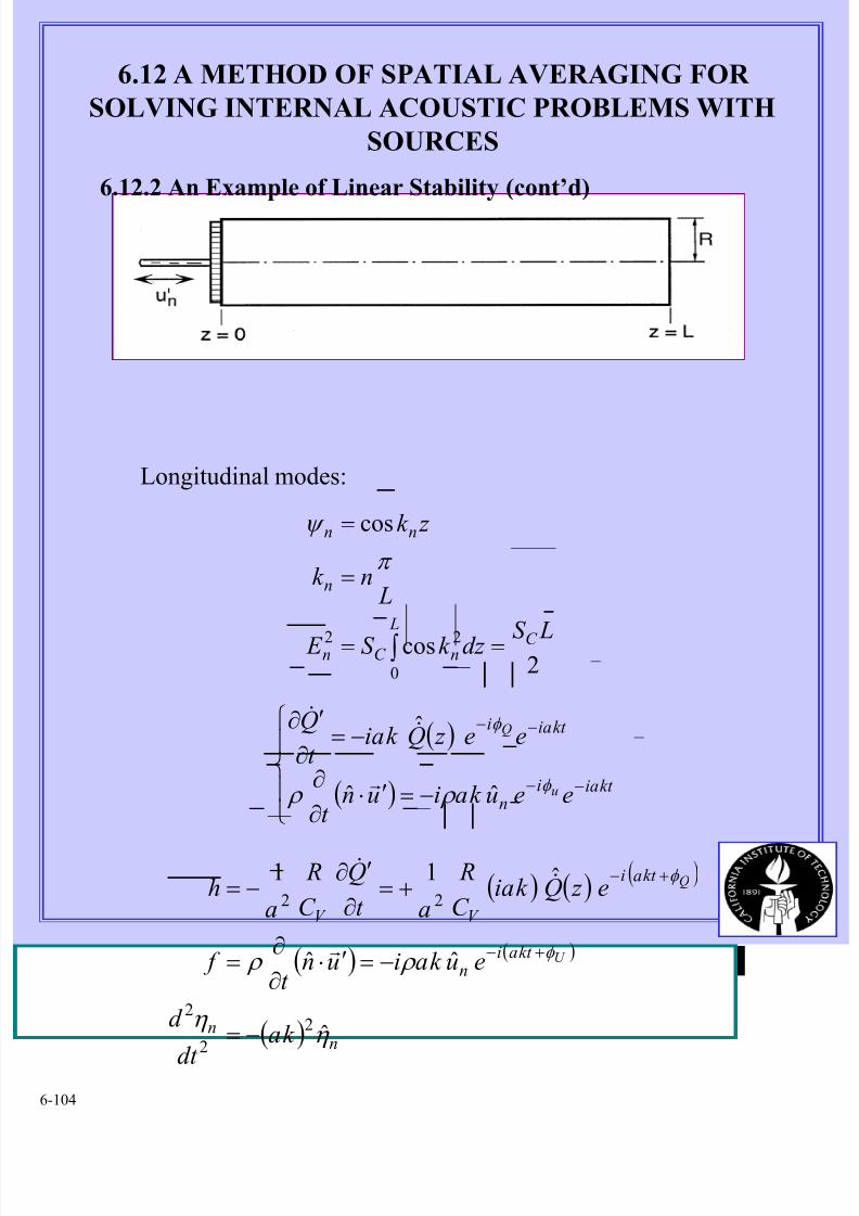
8/11/2019 Fundamentals of Acoustically Coupled Combustions
http://slidepdf.com/reader/full/fundamentals-of-acoustically-coupled-combustions 104/1206-104
6.12.2 An Example of Linear Stability (cont’d)
Longitudinal modes:
2cos
cos
0
22 LS dz k S E
Lnk
z k
C L
nC n
n
nn
==
=
=
∫
π
ψ
( )
( )
−=′⋅∂
∂
−=∂
′∂
−−
−−
kt aiin
kt aii
eeuk aiunt
ee z Qkait
Q
u
Q
φ
φ
ρ ρ ˆˆ
ˆ
r
&&
( ) ( ) ( )
( ) ( )
( ) n
n
kt ain
kt ai
V V
k adt
d
euk aiunt
f
e z Qk aiC
R
at
Q
C
R
ah
U
Q
η
η
ρ ρ φ
φ
ˆ
ˆˆ
ˆ11
2
2
2
22
−=
−=′⋅∂
∂=
+=∂
′∂−=
+−
+−
r
&&
6.12 A METHOD OF SPATIAL AVERAGING FOR
SOLVING INTERNAL ACOUSTIC PROBLEMS WITH
SOURCES
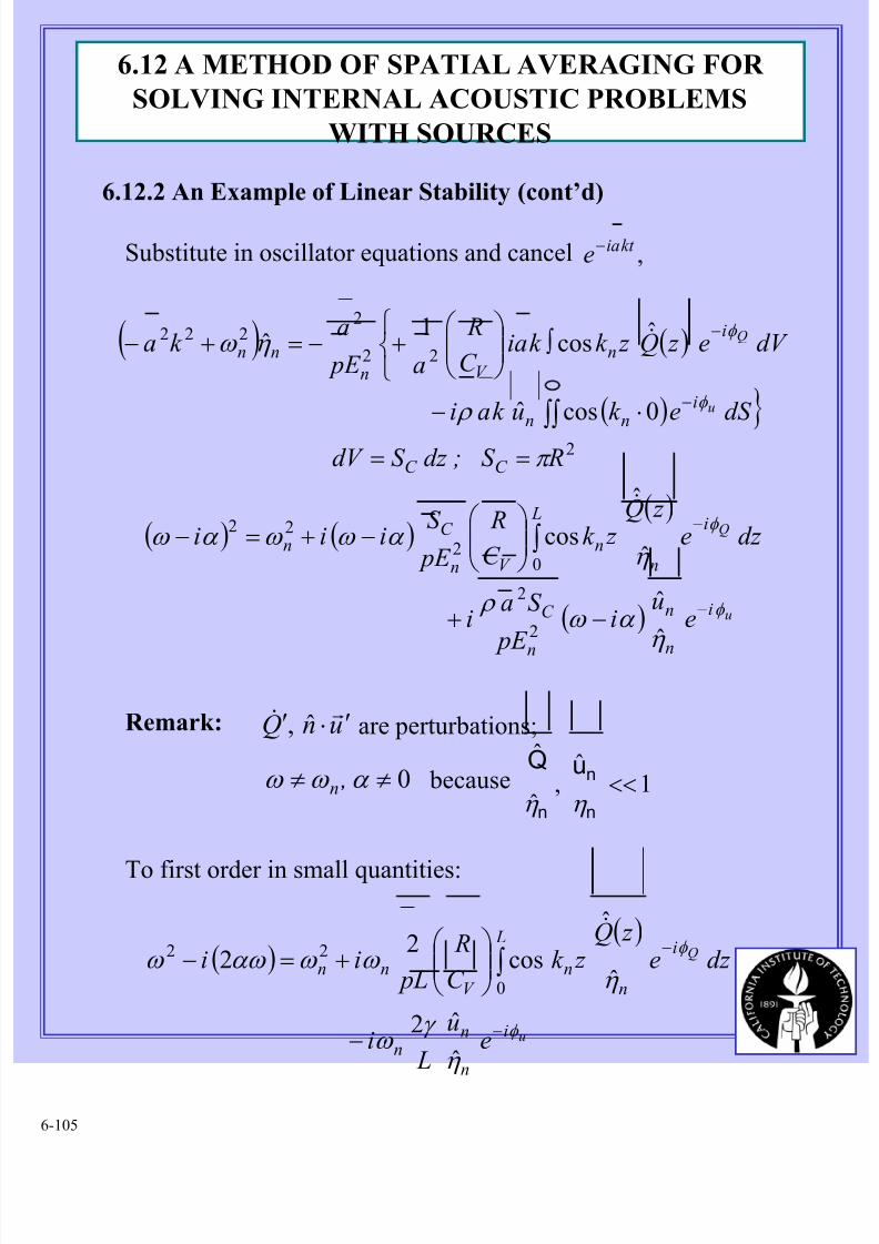
8/11/2019 Fundamentals of Acoustically Coupled Combustions
http://slidepdf.com/reader/full/fundamentals-of-acoustically-coupled-combustions 105/1206-105
6.12.2 An Example of Linear Stability (cont’d)
Substitute in oscillator equations and cancel ,kt aie−
Remark: unQ ′⋅′ r& ˆ, are perturbations;
0≠≠ α ω ω ,n because
To first order in small quantities:
( )( )
u
Q
i
n
nn
Li
nn
V nn
eu
L
i
dz e z Q
z k C
R
L pii
φ
φ
η
γ ω
η ω ω αω ω
−
−
−
+=− ∫
ˆ
ˆ2
ˆ
ˆ
cos2
20
22
&
1ˆ
,ˆ
ˆ
<<n
n
n
uQ
η η
( ) ( )
( ) }
( ) ( )( )
( ) u
Q
u
Q
i
n
n
n
C
Li
nn
V n
C n
C C
i
nn
i
nV n
nn
eu
i
E p
S ai
dz e z Q
z k C
R
E p
S iii
RS ;dz S dV
dS ek uk ai
dV e z Q zk k aiC
R
a E p
ak a
φ
φ
φ
φ
η
α ω ρ
η α ω ω α ω
π
ρ
η ω
−
−
−
−
−+
−+=−
==
⋅−
∫
+−=+−
∫
∫∫
ˆ
ˆ
ˆ
ˆ
cos
0cosˆ
ˆcos1
ˆ
2
2
02
22
2
22
2222
&
&
6.12 A METHOD OF SPATIAL AVERAGING FOR
SOLVING INTERNAL ACOUSTIC PROBLEMS
WITH SOURCES
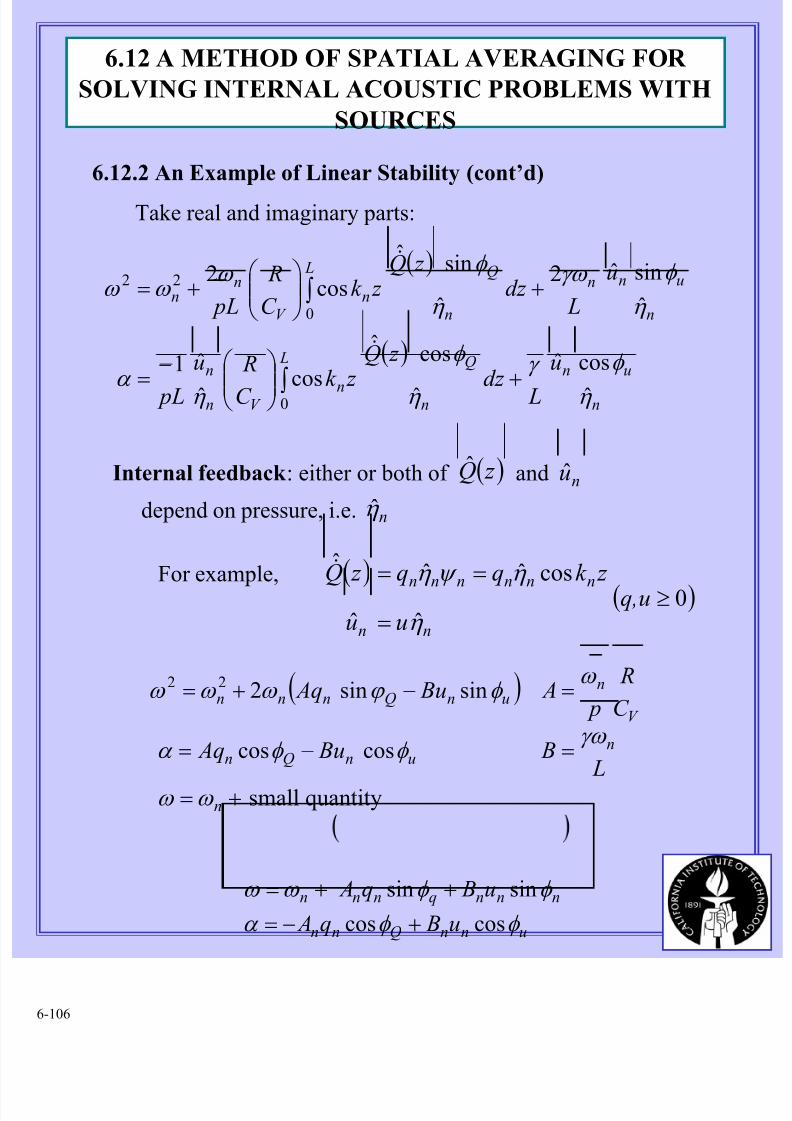
8/11/2019 Fundamentals of Acoustically Coupled Combustions
http://slidepdf.com/reader/full/fundamentals-of-acoustically-coupled-combustions 106/1206-106
Internal feedback : either or both of and
6.12.2 An Example of Linear Stability (cont’d)
Take real and imaginary parts:
( ) z Q
( )
( )
n
un L
n
Q
nV n
n
n
unn L
n
Q
nV
nn
u
Ldz
z Q
z k C
Ru
L p
u
Ldz
z Q z k
C
R
L p
η
φ γ
η
φ
η α
η
φ γω
η
φ ω ω ω
ˆ
cosˆ
ˆ
cosˆ
cosˆ
ˆ1
ˆ
sinˆ2
ˆ
sinˆ
cos2
0
0
22
+
−
=
+
+=
∫
∫
&
&
nu
depend on pressure, i.e. nη ˆ
For example, ( )
nn
nnnnnn
uu
z k qq z Q
η
η ψ η
ˆˆ
cosˆˆˆ
===& ( )0≥uq,
( )
quantitysmall
coscos
sinsin222
+=
=−=
=−+=
n
nunQn
V
nunQnnn
L
B Bu Aq
C
R
p A Bu Aq
ω ω
γω φ φ α
ω φ ϕ ω ω ω
unnQnn
nnnqnnn
u Bq A
u Bq A
φ φ α
φ φ ω ω
coscos
sinsin
+−=
++=
6.12 A METHOD OF SPATIAL AVERAGING FOR
SOLVING INTERNAL ACOUSTIC PROBLEMS WITH
SOURCES
8/11/2019 Fundamentals of Acoustically Coupled Combustions
http://slidepdf.com/reader/full/fundamentals-of-acoustically-coupled-combustions 107/120
8/11/2019 Fundamentals of Acoustically Coupled Combustions
http://slidepdf.com/reader/full/fundamentals-of-acoustically-coupled-combustions 108/1206-108
6.12.3 A General Result for Linear Stability (cont’d)
Special Averaging ⇒ Oscillator Equations
Linear Stability ( linear in and )
{ }∫∫+∫−=
=+
dS f dV h E p
a F
F dt
d
nn
n
n
nnnn
ψ ψ
η ω η
2
2
2
2
2
n F nη nη &
kt ainn
kt ainn e F F e −− == ˆη η
n F ˆ has the general form
( ) ( )
( )nnnnn
i
n
r
nn F i F i F F inˆˆˆˆˆˆ
η ω η η =−=
Substitute:
) ( ) ( )
( ) ( )( )
( ) ( ) ( )
( )n
i
n
r
nn
in
r nn
ni
nr
nnn
F i F i
k a F i F k a
F i F k a
αω αω ω α
ω αω α ω
α ω ω
η η ω
≈<<
−−=−−
−=−−=
−=−
;
ˆˆ2
1;ˆˆ
ˆˆˆˆ
22
222
222
222
n
in
n
n
r n
nn
F
F
η ω α
η ω ω ω
ˆ
ˆ
2
1
ˆ
ˆ
2
1
)(
)(
−=
−=
( )nω ω ≈
6.12 A METHOD OF SPATIAL AVERAGING FOR
SOLVING INTERNAL ACOUSTIC PROBLEMS WITH
SOURCES
8/11/2019 Fundamentals of Acoustically Coupled Combustions
http://slidepdf.com/reader/full/fundamentals-of-acoustically-coupled-combustions 109/1206-109
6.12.3 A General Result for Linear Stability (cont’d)
( )
0
ˆ
ˆ>
n
in F
η
Small amplitude motions are unstable if α > 0
Instability:
This is essentially a generalized form of
Rayleigh’s Criterion for linear behavior
Remarks:
(i) accommodates all linear processes
(ii) The main problem is modeling
(iii) The frequency shift is normally
not important in linear behavior, but is
significant in nonlinear behavior.
n F
nω ω −
6.12 A METHOD OF SPATIAL AVERAGING FOR
SOLVING INTERNAL ACOUSTIC PROBLEMS
WITH SOURCES
8/11/2019 Fundamentals of Acoustically Coupled Combustions
http://slidepdf.com/reader/full/fundamentals-of-acoustically-coupled-combustions 110/1206-110
6.13 APPLICATION OF TIME AVERAGING
• Commonly (not always) unstable oscillations in combustors haveslowly varying amplitude A and phase φ; that is, during one cycle,
or
12
11 <<<<dt d T ;
dt d φ
π τ A
A
where is the period of the oscillation.ω
π τ
21==
f
• The primary intention of the method is to change the
dependent variable from the rapidly varying oscillatoryamplitude ηn (governed by a second order equation) to theslowly varying amplitude A and phase φ (two first-order
equations)
• Two main advantages of the method:
(i) Because the oscillatory motions are removed,
numerical solutions to the equations are much cheaper
and quicker (perhaps several cycles for each interval
of integration)
(ii) The first order equations are convenient for certain
theoretical considerations and for understanding
qualitative behavior
12
;1 <<<<π
δφ δ
A
A
8/11/2019 Fundamentals of Acoustically Coupled Combustions
http://slidepdf.com/reader/full/fundamentals-of-acoustically-coupled-combustions 111/1206-111
(i) Given the oscillations with forcing function ‘small’
of order, µ<< 1:
Procedure:
nnnnn G F µ η ω η ==+ 2&&
Remark: In combustors, µ is of the order of the Mach number of the mean
flow and )1(0~nG
(ii) Write in the equivalent form defining the pairs of
functions and :
( )t nη
( ) ( )( )t t nn φ , A
( ) ( ) ( )( ) ( ) ( ) t t Bt t At t t At nnnnnnnn ω ω φ ω η sincossin +=+=
( ) ( )
( )t A
t Bt
B A
B; A
n
nn
nnn
nnnnnn
1
22
tan
sincos
−=
+=
==
φ
φ φ
A
A A
(iii) One way to proceed follows a physical argument based
on the energy of the oscillator and its change in time.
The mechanical energy of the nth oscillator is the sum
of potential and kinetic energies:
222
2
1
2
1nnnn η η ω &+=E
( ) ( )( )t Bt nn , A
6.13 APPLICATION OF TIME AVERAGING
8/11/2019 Fundamentals of Acoustically Coupled Combustions
http://slidepdf.com/reader/full/fundamentals-of-acoustically-coupled-combustions 112/1206-112
(iv) The time average values of energy and power input
to the oscillator due to action of the force are
( ) ( ) ( )nnnnnnnnnnnn t t t φ ω φ φ ω φ ω ω η +++++= cossincos A A A &&&
(vi) From (ii), the velocity of the oscillator is
t d F F t d t
t nnnn
t
t nn
′=′= ∫∫++ τ τ
η τ
η τ
&&11
E E
n F
where τ is an interval of time-averaging.
(v) Conservation of energy requires that the time-
averaged rate of change of energy equal the time-
averaged rate of work done by on the oscillator:
nnn F dt
d η &=E
Apply the ‘strong’ condition (Krylov and Bogoliubov)
that the velocity is always given by the formula for an
oscillator in force-free notion
( ) ( )( )
( ) ( ) ( ) 0cossin
cos
=+++∗
+=
nnnnnnn
nnnnn
t t
t t t
φ ω φ φ ω
φ ω ω η
A A
A
&&
&
6.13 APPLICATION OF TIME AVERAGING
n F
8/11/2019 Fundamentals of Acoustically Coupled Combustions
http://slidepdf.com/reader/full/fundamentals-of-acoustically-coupled-combustions 113/1206-113
( ) ( )[ ]
dt
d
dt
d
t t
nnn
n
nnn
nnnnnnnn
nnnnn
A A
E
A E
A A E
22
22
222222
2222
2
1
2
1cossin
22
1
2
1
ω
ω
ω φ ω φ ω ω
η ω
=
=
=+++=+= &
(vii) Compute the time averages in (v.)
( )( ) ( )
( ) ( ) ( ) ( ) nnnnnnnnnnnnnnn
nnnnnnnnn
nnnn
F t t t
F t t dt
d
F
=++++−+
=+++
==
φ ω ω φ ω φ ω ω φ ω ω
φ ω ω φ ω ω
η ω η
sinsincos
sincos
2
2
2
A A A
A A
&&
&&
(a)
(b)
( ) t d F t A F F nnnn
t
t
nnn ′+′= ∫
+
φ ω τ
η τ
cos1
&
( ) t d t F dt
d nn
t
t n
n
n ′+′= ∫+
φ ω τ ω
τ
cos1 A
(viii) To find the equation for substitute in the oscillator
equation:
,n
φ &
6.13 APPLICATION OF TIME AVERAGING
8/11/2019 Fundamentals of Acoustically Coupled Combustions
http://slidepdf.com/reader/full/fundamentals-of-acoustically-coupled-combustions 114/1206-114
( )nnnn
nn t F dt
d φ ω
φ ω +=− sin A
( ) t d t F dt
d nn
t
t n
n
nn
′+′−= ∫+
φ ω τ ω
φ τ
sin1
A
Substitute condition (∗), part (vi):
(ix) Time-average over ( ) :, τ +t t
(x) From definitions of and , part (ii):n A n B
( )
( ) t d t F dt
dB
t d t F dt
dA
n
t
t n
n
n
n
t
nn
n
′′−
=
′′=
∫
∫+
+
ω τ ω
ω τ ω
τ
τ
sin1
cos
1
t
6.13.1 Example: Linear Stability
First need to construct representation of the processes,
i.e., n F
nnnn F =+ η ω η 2&&
General form of for linear processes onlyn F
nnnnn E D F η η −−= &
6.13 APPLICATION OF TIME AVERAGING
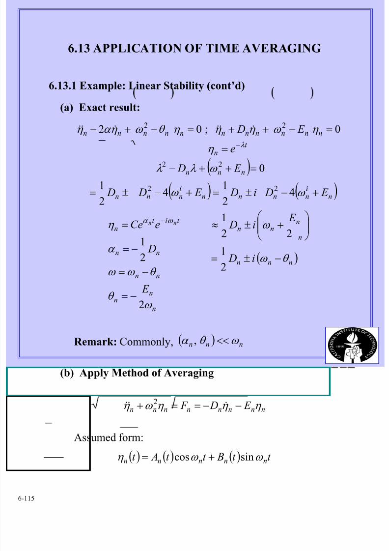
8/11/2019 Fundamentals of Acoustically Coupled Combustions
http://slidepdf.com/reader/full/fundamentals-of-acoustically-coupled-combustions 115/120
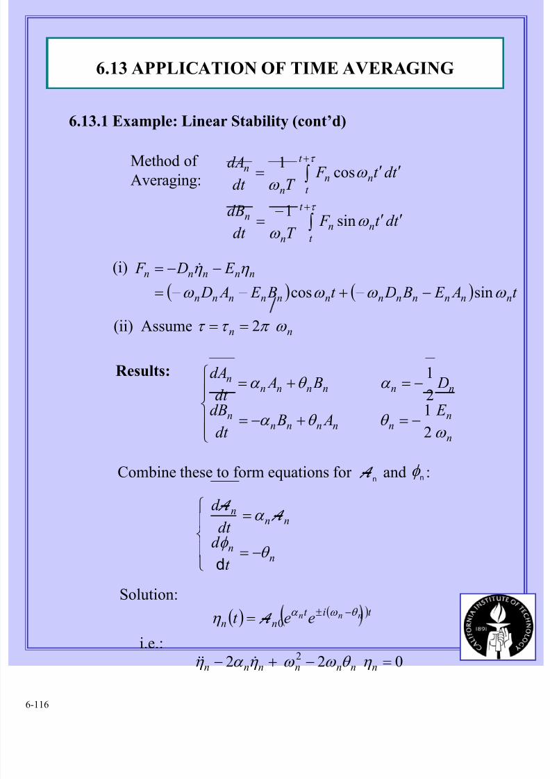
8/11/2019 Fundamentals of Acoustically Coupled Combustions
http://slidepdf.com/reader/full/fundamentals-of-acoustically-coupled-combustions 116/1206-116
6.13.1 Example: Linear Stability (cont’d)
( ) ( ) t A E B Dt B E A D
E D F
nnnnnnnnnnnn
nnnnn
ω ω ω ω
η η
sincos −−+−−=−−= &
( ) ( )t it nn
nnn eet θ ω α
η −±= 0 A
Method of
Averaging:
t d t F T dt
dB
t d t F T dt
dA
n
t
t n
n
n
n
t
t n
n
n
′′−
=
′′=
∫
∫
+
+
ω ω
ω ω
τ
τ
sin1
cos1
(i)
(ii) Assume nn ω π τ τ 2==
−=+−=
−=+=
n
nnnnnn
n
nnnnnnn
E A B
dt
dB
D B A
dt
dA
ω θ θ α
α θ α
2
12
1Results:
−=
=
nn
nnn
t
d dt
d
θ φ
α
d
A A
Combine these to form equations for and :n
A nφ
Solution:
i.e.:
022
2
=−+− nnnnnnn η θ ω ω η α η &&&
6.13 APPLICATION OF TIME AVERAGING
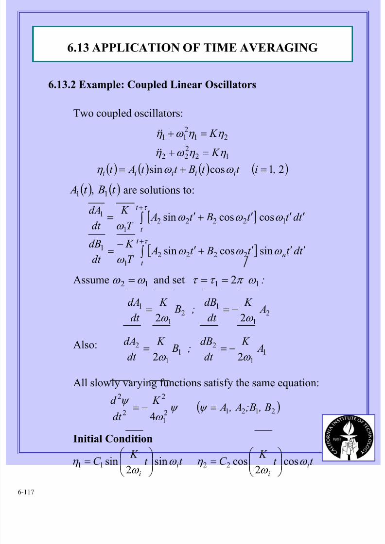
8/11/2019 Fundamentals of Acoustically Coupled Combustions
http://slidepdf.com/reader/full/fundamentals-of-acoustically-coupled-combustions 117/1206-117
[ ]
[ ] t d t t Bt AT
K
dt
dB
t d t t Bt AT
K
dt
dA
n
t
t
t
t
′′′+′−
=
′′′+′=
∫
∫
+
+
ω ω ω ω
ω ω ω ω
τ
τ
sincossin
coscossin
22221
1
122221
1
Also:
6.13.2 Example: Coupled Linear Oscillators
Two coupled oscillators:
( ) ( )t Bt A 11 ,
( ) ( ) ( ) ( )21cossin
12222
21211
,it t Bt t At
K
K
iiiii =+=
=+
=+
ω ω η
η η ω η
η η ω η
&&
&&
are solutions to:
Assume and set12 ω ω = :11 2 ω π τ τ ==
21
12
1
1
22 A
K
dt
dB; B
K
dt
dA
ω ω −==
11
21
1
2
22 A
K
dt
dB; B
K
dt
dA
ω ω −==
All slowly varying functions satisfy the same equation:
( )212121
2
2
2
4 B ,;B A , A
K
dt
d =−= ψ ψ
ω
ψ
Initial Condition
t t
K
C tt
K
C ii
ii ω ω η ω ω η cos2cossin2sin 2211
=
=
6.13 APPLICATION OF TIME AVERAGING
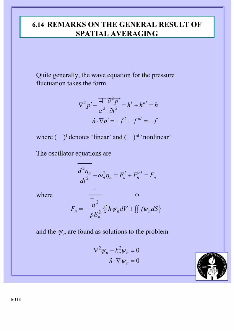
8/11/2019 Fundamentals of Acoustically Coupled Combustions
http://slidepdf.com/reader/full/fundamentals-of-acoustically-coupled-combustions 118/1206-118
6.14 REMARKS ON THE GENERAL RESULT OF
SPATIAL AVERAGING
Quite generally, the wave equation for the pressure
fluctuation takes the form
f f f pn
hhh
t
p
a
p
nl l
nl l
−=−−=′∇⋅
=+=
∂
′∂−′∇
ˆ
12
2
2
2
where ( )l denotes ‘linear’ and ( )nl ‘nonlinear’
The oscillator equations are
nnl
nl
nnnn F F F
dt
d =+=+ η ω η 2
2
2
where
{ }∫ ∫∫+−= dS f dV h E p
a F nn
n
n ψ ψ 2
2
and the are found as solutions to the problemnψ
0ˆ
022
=∇⋅
=+∇
n
nnn
n
k
ψ
ψ ψ
8/11/2019 Fundamentals of Acoustically Coupled Combustions
http://slidepdf.com/reader/full/fundamentals-of-acoustically-coupled-combustions 119/1206-119
Thus splits into a sum of linear and nonlinear parts
{ } { }∫ ∫∫∫ ∫∫ +−+−= dS f dV h E p
adS f dV h
E p
a F n
nl n
nl
n
nl
nl
n
n ψ ψ ψ ψ 2
2
2
2
n F
If there is no linear coupling between modes
{ }∫ ∫∫+−+= dS f dV h E p
a F n
nl n
nl
n
nnnnnn ψ ψ η θ ω η α 2
2
22 &
and
{ }∫ ∫∫+−=+ dS f dV h E p
an
l n
l
n
nnnnn ψ ψ η θ ω η α 2
2
2&
is the formula for computing and .nα nθ
Note: Linear coupling between modes can be removed by formal transformation (see § 6.10.2)
6.14 REMARKS ON THE GENERAL RESULT OF
SPATIAL AVERAGING
8/11/2019 Fundamentals of Acoustically Coupled Combustions
http://slidepdf.com/reader/full/fundamentals-of-acoustically-coupled-combustions 120/120
End of Section VI