General-Order Many-Body Green s Function Method

General-Order Many-Body Green’s Function MethodSo Hirata,*,† Matthew R. Hermes,† Jack Simons,‡ and J. V. Ortiz§

†Department of Chemistry, University of Illinois at Urbana−Champaign, Urbana, Illinois 61801, United States‡Department of Chemistry, University of Utah, Salt Lake City, Utah 84112, United States§Department of Chemistry and Biochemistry, Auburn University, Auburn, Alabama 36849-5312, United States

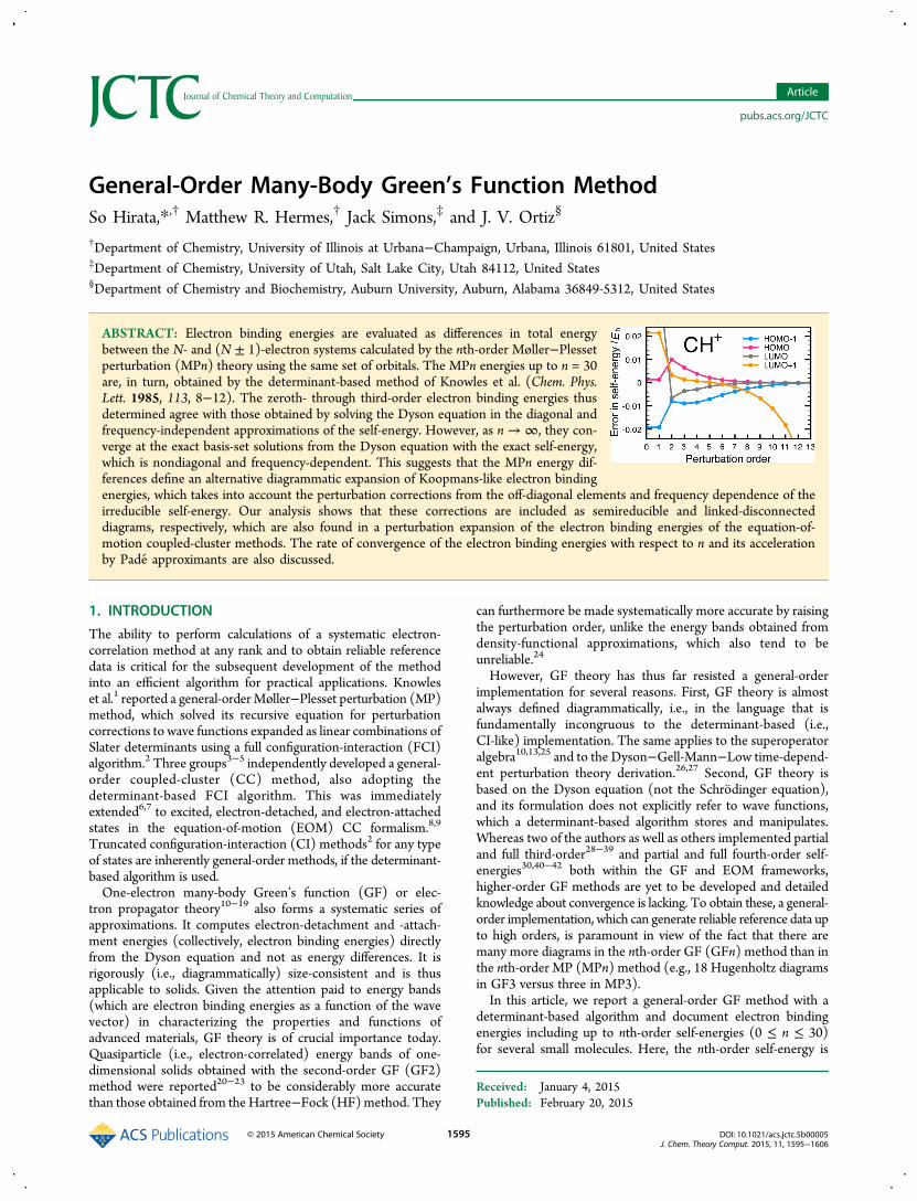
ABSTRACT: Electron binding energies are evaluated as differences in total energybetween the N- and (N ± 1)-electron systems calculated by the nth-order Møller−Plessetperturbation (MPn) theory using the same set of orbitals. The MPn energies up to n = 30are, in turn, obtained by the determinant-based method of Knowles et al. (Chem. Phys.Lett. 1985, 113, 8−12). The zeroth- through third-order electron binding energies thusdetermined agree with those obtained by solving the Dyson equation in the diagonal andfrequency-independent approximations of the self-energy. However, as n → ∞, they con-verge at the exact basis-set solutions from the Dyson equation with the exact self-energy,which is nondiagonal and frequency-dependent. This suggests that the MPn energy dif-ferences define an alternative diagrammatic expansion of Koopmans-like electron bindingenergies, which takes into account the perturbation corrections from the off-diagonal elements and frequency dependence of theirreducible self-energy. Our analysis shows that these corrections are included as semireducible and linked-disconnecteddiagrams, respectively, which are also found in a perturbation expansion of the electron binding energies of the equation-of-motion coupled-cluster methods. The rate of convergence of the electron binding energies with respect to n and its accelerationby Pade approximants are also discussed.

1. INTRODUCTION

The ability to perform calculations of a systematic electron-correlation method at any rank and to obtain reliable referencedata is critical for the subsequent development of the methodinto an efficient algorithm for practical applications. Knowleset al.1 reported a general-orderMøller−Plesset perturbation (MP)method, which solved its recursive equation for perturbationcorrections to wave functions expanded as linear combinations ofSlater determinants using a full configuration-interaction (FCI)algorithm.2 Three groups3−5 independently developed a general-order coupled-cluster (CC) method, also adopting thedeterminant-based FCI algorithm. This was immediatelyextended6,7 to excited, electron-detached, and electron-attachedstates in the equation-of-motion (EOM) CC formalism.8,9

Truncated configuration-interaction (CI) methods2 for any typeof states are inherently general-order methods, if the determinant-based algorithm is used.One-electron many-body Green’s function (GF) or elec-

tron propagator theory10−19 also forms a systematic series ofapproximations. It computes electron-detachment and -attach-ment energies (collectively, electron binding energies) directlyfrom the Dyson equation and not as energy differences. It isrigorously (i.e., diagrammatically) size-consistent and is thusapplicable to solids. Given the attention paid to energy bands(which are electron binding energies as a function of the wavevector) in characterizing the properties and functions ofadvanced materials, GF theory is of crucial importance today.Quasiparticle (i.e., electron-correlated) energy bands of one-dimensional solids obtained with the second-order GF (GF2)method were reported20−23 to be considerably more accuratethan those obtained from theHartree−Fock (HF)method. They

can furthermore be made systematically more accurate by raisingthe perturbation order, unlike the energy bands obtained fromdensity-functional approximations, which also tend to beunreliable.24

However, GF theory has thus far resisted a general-orderimplementation for several reasons. First, GF theory is almostalways defined diagrammatically, i.e., in the language that isfundamentally incongruous to the determinant-based (i.e.,CI-like) implementation. The same applies to the superoperatoralgebra10,13,25 and to the Dyson−Gell-Mann−Low time-depend-ent perturbation theory derivation.26,27 Second, GF theory isbased on the Dyson equation (not the Schrodinger equation),and its formulation does not explicitly refer to wave functions,which a determinant-based algorithm stores and manipulates.Whereas two of the authors as well as others implemented partialand full third-order28−39 and partial and full fourth-order self-energies30,40−42 both within the GF and EOM frameworks,higher-order GF methods are yet to be developed and detailedknowledge about convergence is lacking. To obtain these, a general-order implementation, which can generate reliable reference data upto high orders, is paramount in view of the fact that there aremany more diagrams in the nth-order GF (GFn) method than inthe nth-order MP (MPn) method (e.g., 18 Hugenholtz diagramsin GF3 versus three in MP3).In this article, we report a general-order GF method with a

determinant-based algorithm and document electron bindingenergies including up to nth-order self-energies (0 ≤ n ≤ 30)for several small molecules. Here, the nth-order self-energy is

Received: January 4, 2015Published: February 20, 2015

Article

pubs.acs.org/JCTC

© 2015 American Chemical Society 1595 DOI: 10.1021/acs.jctc.5b00005J. Chem. Theory Comput. 2015, 11, 1595−1606

pubs.acs.org/JCTC

http://dx.doi.org/10.1021/acs.jctc.5b00005

defined as the difference in the MPn energy between the N- and(N ± 1)-electron systems, all of which are described with the HForbitals and orbitals energies of the N-electron system. TheseMPn energies are, in turn, calculated at any n by the general-orderMP method of Knowles et al.1 We call this procedure ΔMPn,which must not be confused with the simple difference in MPnenergies obtained with the HF orbitals individually determinedfor N- and (N ± 1)-electron systems; nowhere in a ΔMPn cal-culation for a closed-shell molecule is a HF calculation of anopen-shell molecule performed, which tends to suffer from spincontamination.43 While ΔMPn implemented algebraically wasused by Chong et al.44−46 in their analysis of GFn at low orders,little is known about its behavior at n > 3.For 0 ≤ n ≤ 3, the electron binding energies obtained from

ΔMPn are identified as the values determined with the self-energies in the diagonal approximation and evaluated at the HForbital energies, namely, in the frequency-independent approx-imation. However, as n→∞, they converge at the exact basis-setvalues obtained with FCI or with the full GF method using theexact self-energy, which is nondiagonal and frequency-dependent.This suggests that ΔMPn includes the perturbation correctionsdue to the off-diagonal elements and frequency dependence ofthe irreducible self-energy exactly at n = ∞. These correctionsare shown to be represented as semireducible and linked-disconnected diagrams, respectively, according to our analysis oflow-order examples. While it is well-known that a perturbationexpansion of the nondiagonal, frequency-dependent self-energyis convergent at exactness, we show that a perturbation expansionof the diagonal, frequency-independent self-energy is also con-vergent at the same limit insofar as these new classes of diagramsare taken into account. We furthermore show that a perturbationexpansion of the electron binding energies obtained from theEOM-CC methods also contains the same classes of diagrams.Hence, ΔMPn suggests an alternative perturbation approach

to GF theory with a potentially streamlined algorithm, whichdoes not involve diagonalization or self-consistent solution of theDyson equation, while converging at the exact limits. Its draw-backs are the reduced applicability to just Koopmans-like finalstates and the inability to resist divergence, as this ability isconferred by a frequency-dependent self-energy. In this work,therefore, we also numerically monitor the electron bindingenergies of ΔMPn for a few molecules as a function of n toexamine their convergence rates and whether the correctconverged limits can be deduced from divergent series. We showthat Pade approximants can extrapolate the correct converged limitwithin a fewmEh from divergent series, although it proves to be lesseffective in accelerating the convergence rates elsewhere.

2. THEORYThroughout this article, atomic units are adopted. We use i, j, k, l,m, and n (a, b, c, and d) to label occupied (virtual) orbitals in thespin-restricted HF determinant of an N-electron system in itsground state (N is an even number) and p, q, r, and s to signifyeither type of orbitals. We furthermore employ x and y todesignate an appropriate type of orbitals from which an electronis removed or added. Unless otherwise noted, all orbitals refer tocanonical HF spin-orbitals.2.1. One-ElectronMany-BodyGreen’s Function theory.

The central equation of GF theory is the Dyson equation10−19

ω ω ω ω ωΣ= +G G G G( ) ( ) ( ) ( ) ( )0 0 (1)

which relates the exact one-electron Green’s function, G(ω),with the zeroth-order (in our case, HF) one-electron Green’s

function, G0(ω), through Dyson self-energy, Σ(ω). In a finitebasis set, they all are L-by-L matrices, where L is the number oforbitals, and are dependent on frequency, ω.In the basis of the HF orbitals, the matrix elements of the exact

and HF Green’s functions are given, respectively, by

∑

∑

ωω

ω

=⟨ Ψ | | Ψ ⟩⟨ Ψ | | Ψ ⟩

− −

+⟨ Ψ | | Ψ ⟩⟨ Ψ | | Ψ ⟩

− −

† − −

−

+ + †

+

x yE E

y xE E

G{ ( )}( )

( )

xyn

N Nn

Nn

N

N Nn

n

N Nn

Nn

N

Nn

N

01 1

0

01

01 1

01

0 (2)

ωδ

ω=

− ϵG{ ( )}xy

xy

x0

(3)

where †x creates an electron in the xth orbital, x annihilates thesame, NΨn is the exact wave function of the nth state (n = 0 beingthe ground state) of the N-electron system, NEn is the exactenergy of the same state, and ϵx is the energy of the xth orbital.Hence, G(ω) has poles at exact negative electron-detachment

energies (NE0 − N−1En) and exact negative electron-attachmentenergies (N+1En − NE0), whereas G0(ω) has poles at the energiesof the HF orbitals, which are related to the electron-detachmentand -attachment energies of HF theory in the Koopmansapproximation. A bound anionic state is thus often foreshadowedby a negative, virtual, HF orbital energy.Multiplying eq 1 with G0

−1(ω) from the left and G−1(ω) fromthe right, we obtain the inverse Dyson equation

ω ω ωΣ= +− −G G( ) ( ) ( )01 1

(4)

Since G(ω) diverges at an exact electron binding energy, say ω

ω ω ωΣ= = −− −G G0 det{ ( )} det{ ( ) ( )}10

1(5)

One way to solve eq 5 is to use a new set of orbitals that bringsG−1(ω) into a diagonal form. Since

ϵω ω= −−G 1( )01

(6)

with {ϵ}xy = δxyϵx in the basis of the HF orbitals, the new orbitalsdiagonalize ϵ +Σ(ω) also. Let Σx(ω) be the xth diagonal elementof ϵ + Σ(ω) in this new basis. Equation 5 then simplifies to

∏ ω ω= − Σ0 { ( )}x

x(7)

or

ω ω= Σ ( )x (8)

which is to be solved for ω by bringing it to self-consistencybetween the left- and right-hand sides (whereupon the xth orbitalbecomes a Dyson orbital).To distinguish from approximate solutions to be discussed

below, we call the solution of the above equation the non-diagonal, self-consistent solution. The recursive structure of theinverse Dyson equation allows a single eq 8 to have multipleroots, corresponding not only to the fundamental (Koopmans)but also to satellite (shakeup) transitions.In the diagonal approximation, the off-diagonal elements of

G−1(ω) [thusΣ(ω)] in the basis of the HF orbitals are neglected.Then, eq 5 reduces to

∏ ω ω= − ϵ − Σ0 { ( )}x

x x(9)

Journal of Chemical Theory and Computation Article

DOI: 10.1021/acs.jctc.5b00005J. Chem. Theory Comput. 2015, 11, 1595−1606

1596


where Σx(ω) is the xth diagonal element ofΣ(ω). This leads to arecursive equation

ω ω= ϵ + Σ ( )x x (10)

which is, again, to be solved forω, making the left- and right-handsides self-consistent. We call this the diagonal approximation.47

A simpler alternative to seeking self-consistent solutions is toevaluate the self-energy at ω = ϵx, that is

ω = ϵ + Σ ϵ( )x x x (11)

We call this method the diagonal, frequency-independent(ω-independent) approximation.47 This may be justified whenϵx is sufficiently far from any of the poles of Σx(ω), where thelatter is nearly constant with ω. It gives the energies of thefundamental transitions only.2.2. Feynman−Goldstone Diagrams. The self-energy in

the basis of the HF orbitals is expanded into a diagrammaticperturbation series.26,27 In the diagonal approximation, we canwrite

∑ω ω= Σ=

( )n

m

n

xm( )

0

( )

(12)

where ω(n) is the electron binding energy in the nth-orderperturbation theory and Σx

(m)(ω) is the mth-order perturbationcorrection to the self-energy. The Møller−Plesset partitioningof the Hamiltonian, = + H H V0 , is used, where H0 is the sum

of the Fock operators and V is the fluctuation potential. Thispartitioning is consistent with G0(ω) being defined by HFtheory. Hence, Σx

(0)(ω) = ϵx.Themth-order correction to the self-energy,Σx

(m), is the sum ofcontributions from all Feynman−Goldstone diagrams withm interaction ( V ) vertexes that are linked, irreducible, andopen with exactly two external edges or “stubs”.26,27 Thesediagrams are then interpreted expediently according tothe established rules26,27 into algebraic expressions of Σx

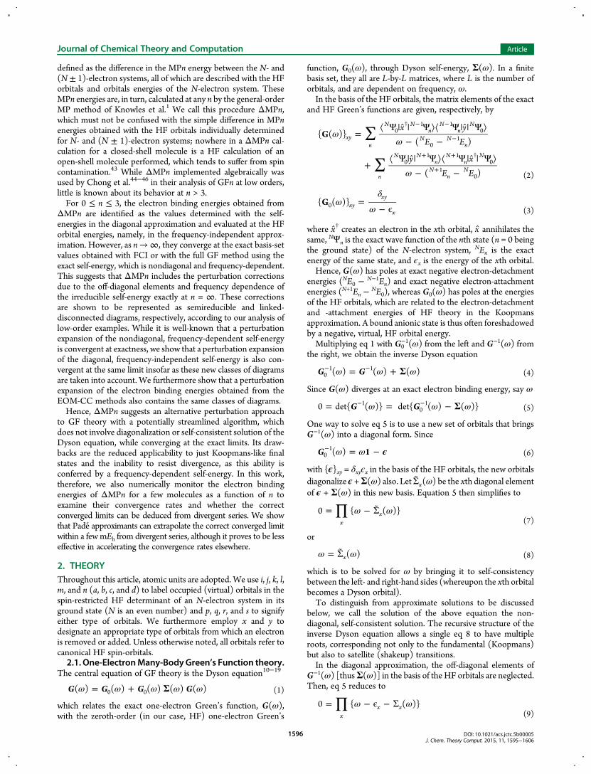
(m).These rules are rigorously derivable by the Dyson−Gell-Mann−Low time-dependent perturbation theory26,27 and are mathe-matically equivalent to the superoperator algebra.10,13,18,25 Thediagrammatic method, however, can provide unique, graphicalinformation about size consistency of GF theory,48−50 the recur-sive structure of the Dyson equation,26,50 the concept of edgeinsertion,50−52 etc.Figure 1 draws the MP2 energy diagram as diagram A. The

closed, linked nature of this diagram ensures the extensivity of the

MP2 energy.48,49,53 Specifically, each four-edge vertex (repre-senting a two-electron integral) contributes a factor of V−1 to thevolume (V) dependence of the diagram, and each independentinternal edge (a line connecting two vertexes), a factor of V. Ofthe four internal edges in diagram A, only three are independentwith the fourth determined by the momentum conservation law.

Together, diagram A scales as V−2V3 = V and is thermodynami-cally extensive.Self-energy diagrams can be generated by “cutting an edge” of

closed diagrams with the same order (plus additional ones, insome instances31) in all topologically distinct ways. Cutting theith edge of diagram A, we obtain self-energy diagram B. Cuttingthe bth edge spawns self-energy diagram C. The edge that hasbeen cut becomes two external edges, which do not contribute tothe V dependence of the diagram. Diagrams B and C, therefore,scale as V−2V2 = V0 and represent thermodynamically intensivequantities.These diagrams are directly translated to algebraic expressions

according to the established rules found in, e.g., Mattuck.26 Forfuture use, we translate diagrams B and C into algebraic forms

∑ωω

Σ =⟨ || ⟩⟨ || ⟩+ ϵ − ϵ − ϵxj ab ab xj

( )12x

j a b j a b

(2B)

, , (13)

∑ωω

Σ =⟨ || ⟩⟨ || ⟩+ ϵ − ϵ − ϵij ax ax ij

( )12x

i j a a i j

(2C)

, , (14)

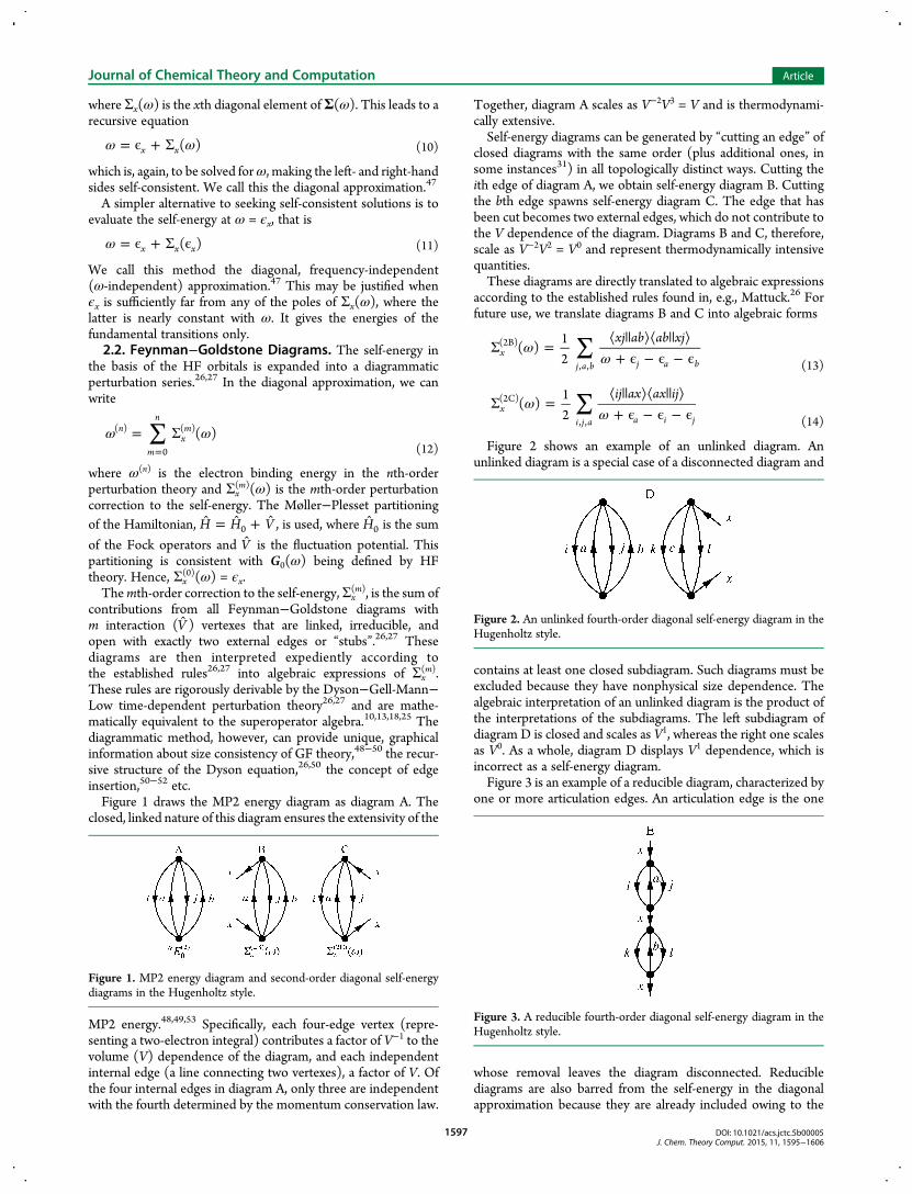
Figure 2 shows an example of an unlinked diagram. Anunlinked diagram is a special case of a disconnected diagram and

contains at least one closed subdiagram. Such diagrams must beexcluded because they have nonphysical size dependence. Thealgebraic interpretation of an unlinked diagram is the product ofthe interpretations of the subdiagrams. The left subdiagram ofdiagram D is closed and scales as V1, whereas the right one scalesas V0. As a whole, diagram D displays V1 dependence, which isincorrect as a self-energy diagram.Figure 3 is an example of a reducible diagram, characterized by

one or more articulation edges. An articulation edge is the one

whose removal leaves the diagram disconnected. Reduciblediagrams are also barred from the self-energy in the diagonalapproximation because they are already included owing to the

Figure 1. MP2 energy diagram and second-order diagonal self-energydiagrams in the Hugenholtz style.

Figure 2. An unlinked fourth-order diagonal self-energy diagram in theHugenholtz style.

Figure 3. A reducible fourth-order diagonal self-energy diagram in theHugenholtz style.



1597


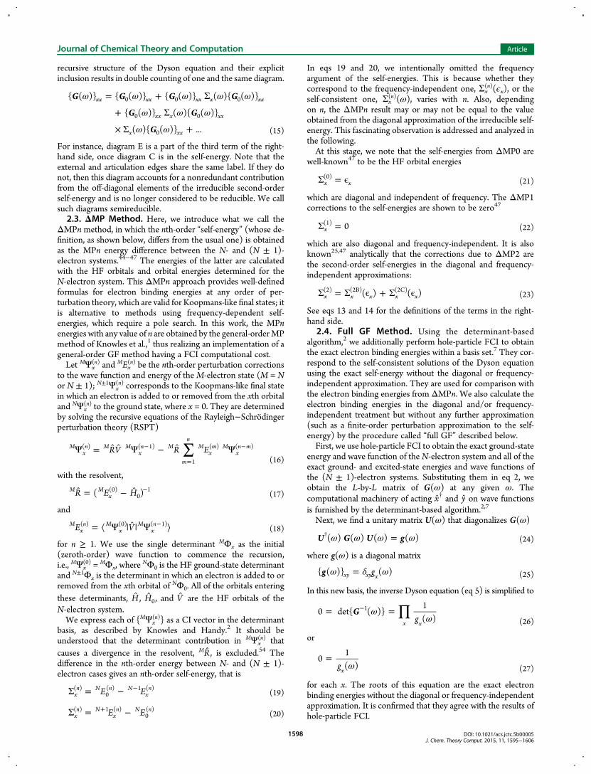
recursive structure of the Dyson equation and their explicitinclusion results in double counting of one and the same diagram.

ω ω ω ω ω

ω ω ω

ω ω

= + Σ

+ Σ

× Σ +

G G G G

G G

G

{ ( )} { ( )} { ( )} ( ){ ( )}

{ ( )} ( ){ ( )}

( ){ ( )} ...

xx xx xx x xx

xx x xx

x xx

0 0 0

0 0

0 (15)

For instance, diagram E is a part of the third term of the right-hand side, once diagram C is in the self-energy. Note that theexternal and articulation edges share the same label. If they donot, then this diagram accounts for a nonredundant contributionfrom the off-diagonal elements of the irreducible second-orderself-energy and is no longer considered to be reducible. We callsuch diagrams semireducible.2.3. ΔMP Method. Here, we introduce what we call the

ΔMPn method, in which the nth-order “self-energy” (whose de-finition, as shown below, differs from the usual one) is obtainedas the MPn energy difference between the N- and (N ± 1)-electron systems.44−47 The energies of the latter are calculatedwith the HF orbitals and orbital energies determined for theN-electron system. This ΔMPn approach provides well-definedformulas for electron binding energies at any order of per-turbation theory, which are valid for Koopmans-like final states; itis alternative to methods using frequency-dependent self-energies, which require a pole search. In this work, the MPnenergies with any value of n are obtained by the general-orderMPmethod of Knowles et al.,1 thus realizing an implementation of ageneral-order GF method having a FCI computational cost.Let MΨx

(n) and MEx(n) be the nth-order perturbation corrections

to the wave function and energy of theM-electron state (M = Nor N ± 1); N±1Ψx

(n) corresponds to the Koopmans-like final statein which an electron is added to or removed from the xth orbitaland NΨx

(n) to the ground state, where x = 0. They are determinedby solving the recursive equations of the Rayleigh−Schrodingerperturbation theory (RSPT)

∑Ψ = Ψ − Ψ−

=

−RV R EMxn M M

xn M

m

nM

xm M

xn m( ) ( 1)

1

( ) ( )

(16)

with the resolvent,

= − −R E H( )M Mx(0)

01

(17)

and

= ⟨ Ψ | | Ψ ⟩−E VMx

n Mx

Mxn( ) (0) ( 1)

(18)

for n ≥ 1. We use the single determinant MΦx as the initial(zeroth-order) wave function to commence the recursion,i.e., MΨx

(0) = MΦx, whereNΦ0 is the HF ground-state determinant

and N±1Φx is the determinant in which an electron is added to orremoved from the xth orbital of NΦ0. All of the orbitals enteringthese determinants, H , H0, and V are the HF orbitals of theN-electron system.We express each of {MΨx

(n)} as a CI vector in the determinantbasis, as described by Knowles and Handy.2 It should beunderstood that the determinant contribution in MΨx

(n) thatcauses a divergence in the resolvent, M R , is excluded.54 Thedifference in the nth-order energy between N- and (N ± 1)-electron cases gives an nth-order self-energy, that is

Σ = − −E Exn N n N

xn( )

0( ) 1 ( )

(19)

Σ = −+ E Exn N

xn N n( ) 1 ( )

0( )

(20)

In eqs 19 and 20, we intentionally omitted the frequencyargument of the self-energies. This is because whether theycorrespond to the frequency-independent one, Σx

(n)(ϵx), or theself-consistent one, Σx

(n)(ω), varies with n. Also, dependingon n, the ΔMPn result may or may not be equal to the valueobtained from the diagonal approximation of the irreducible self-energy. This fascinating observation is addressed and analyzed inthe following.At this stage, we note that the self-energies from ΔMP0 are

well-known47 to be the HF orbital energies

Σ = ϵx x(0)

(21)

which are diagonal and independent of frequency. The ΔMP1corrections to the self-energies are shown to be zero47

Σ = 0x(1)

(22)

which are also diagonal and frequency-independent. It is alsoknown25,47 analytically that the corrections due to ΔMP2 arethe second-order self-energies in the diagonal and frequency-independent approximations:

Σ = Σ ϵ + Σ ϵ( ) ( )x x x x x(2) (2B) (2C)

(23)

See eqs 13 and 14 for the definitions of the terms in the right-hand side.

2.4. Full GF Method. Using the determinant-basedalgorithm,2 we additionally perform hole-particle FCI to obtainthe exact electron binding energies within a basis set.7 They cor-respond to the self-consistent solutions of the Dyson equationusing the exact self-energy without the diagonal or frequency-independent approximation. They are used for comparison withthe electron binding energies from ΔMPn. We also calculate theelectron binding energies in the diagonal and/or frequency-independent treatment but without any further approximation(such as a finite-order perturbation approximation to the self-energy) by the procedure called “full GF” described below.First, we use hole-particle FCI to obtain the exact ground-state

energy and wave function of the N-electron system and all of theexact ground- and excited-state energies and wave functions ofthe (N ± 1)-electron systems. Substituting them in eq 2, weobtain the L-by-L matrix of G(ω) at any given ω. Thecomputational machinery of acting †x and y on wave functionsis furnished by the determinant-based algorithm.2,7

Next, we find a unitary matrix U(ω) that diagonalizes G(ω)

ω ω ω ω=†U G U g( ) ( ) ( ) ( ) (24)

where g(ω) is a diagonal matrix

ω δ ω=g g{ ( )} ( )xy xy x (25)

In this new basis, the inverse Dyson equation (eq 5) is simplified to

∏ωω

= =−Gg

0 det{ ( )}1( )x x

1

(26)

or

ω=

g0

1( )x (27)

for each x. The roots of this equation are the exact electronbinding energies without the diagonal or frequency-independentapproximation. It is confirmed that they agree with the results ofhole-particle FCI.



1598


In the basis of the HF orbitals, G−1(ω) is obtained by the backtransformation

ω ω ω ω=− − †G U g U( ) ( ) ( ) ( )1 1(28)

where g−1(ω) is the diagonal matrix whose xth diagonal ele-ment is {gx(ω)}

−1. The diagonal approximation neglects all off-diagonal elements of G−1(ω) in the basis of the HF orbitals. Theinverse Dyson equation then becomes

∏ ω ω ω= − †U g U0 { ( ) ( ) ( )}x

xx1

(29)

or

ω ω ω= − †U g U0 { ( ) ( ) ( )}xx1

(30)

for each x. The roots of this equation correspond to the solutionsof the Dyson equation using the exact self-energy in the diagonalapproximation.The electron binding energies in the diagonal, frequency-

independent approximation are evaluated by

ω = ϵ + Σ ϵ( )x x x (31)

= ϵ − ϵ ϵ ϵ− †U g U{ ( ) ( ) ( )}x x x x xx1

(32)

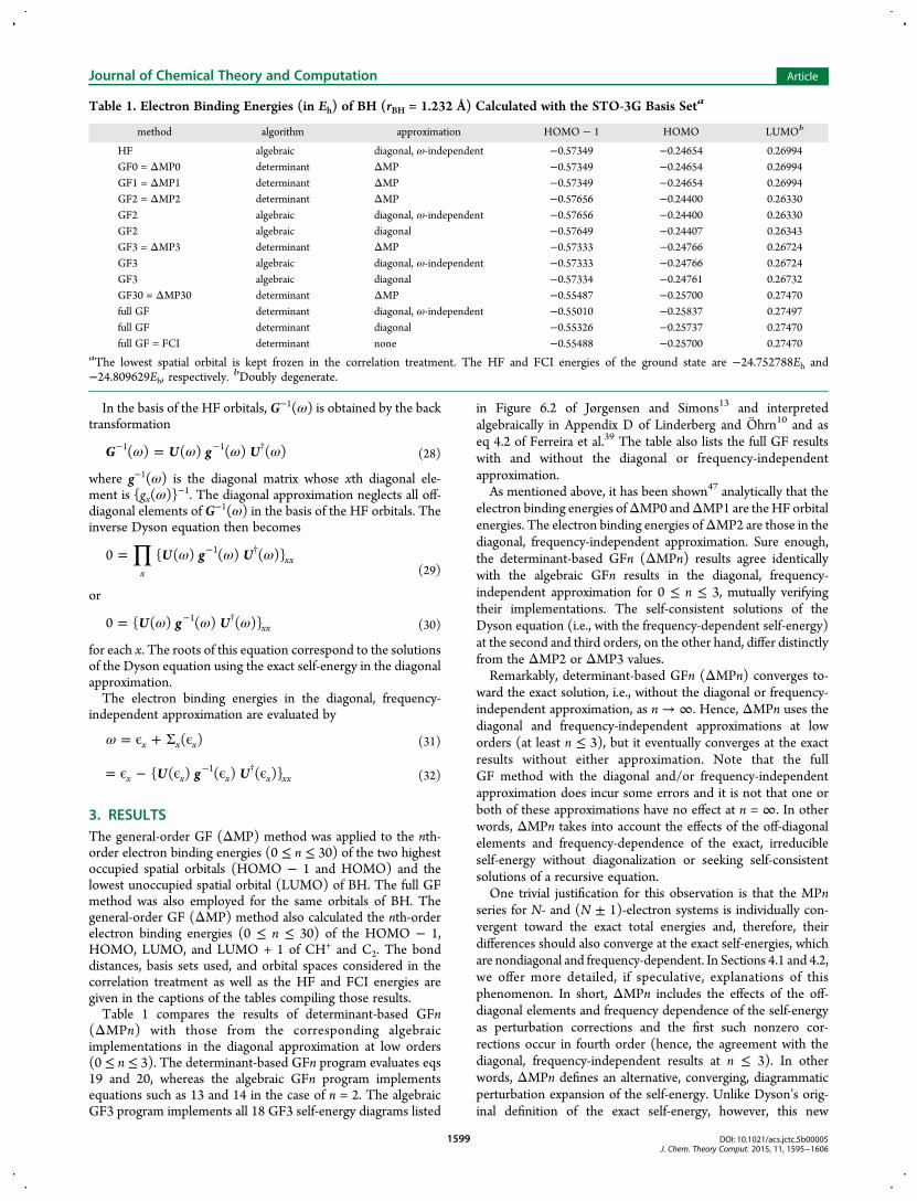
3. RESULTSThe general-order GF (ΔMP) method was applied to the nth-order electron binding energies (0 ≤ n ≤ 30) of the two highestoccupied spatial orbitals (HOMO − 1 and HOMO) and thelowest unoccupied spatial orbital (LUMO) of BH. The full GFmethod was also employed for the same orbitals of BH. Thegeneral-order GF (ΔMP) method also calculated the nth-orderelectron binding energies (0 ≤ n ≤ 30) of the HOMO − 1,HOMO, LUMO, and LUMO + 1 of CH+ and C2. The bonddistances, basis sets used, and orbital spaces considered in thecorrelation treatment as well as the HF and FCI energies aregiven in the captions of the tables compiling those results.Table 1 compares the results of determinant-based GFn

(ΔMPn) with those from the corresponding algebraicimplementations in the diagonal approximation at low orders(0 ≤ n ≤ 3). The determinant-based GFn program evaluates eqs19 and 20, whereas the algebraic GFn program implementsequations such as 13 and 14 in the case of n = 2. The algebraicGF3 program implements all 18 GF3 self-energy diagrams listed

in Figure 6.2 of Jørgensen and Simons13 and interpretedalgebraically in Appendix D of Linderberg and Ohrn10 and aseq 4.2 of Ferreira et al.39 The table also lists the full GF resultswith and without the diagonal or frequency-independentapproximation.As mentioned above, it has been shown47 analytically that the

electron binding energies ofΔMP0 andΔMP1 are theHF orbitalenergies. The electron binding energies ofΔMP2 are those in thediagonal, frequency-independent approximation. Sure enough,the determinant-based GFn (ΔMPn) results agree identicallywith the algebraic GFn results in the diagonal, frequency-independent approximation for 0 ≤ n ≤ 3, mutually verifyingtheir implementations. The self-consistent solutions of theDyson equation (i.e., with the frequency-dependent self-energy)at the second and third orders, on the other hand, differ distinctlyfrom the ΔMP2 or ΔMP3 values.Remarkably, determinant-based GFn (ΔMPn) converges to-

ward the exact solution, i.e., without the diagonal or frequency-independent approximation, as n → ∞. Hence, ΔMPn uses thediagonal and frequency-independent approximations at loworders (at least n ≤ 3), but it eventually converges at the exactresults without either approximation. Note that the fullGF method with the diagonal and/or frequency-independentapproximation does incur some errors and it is not that one orboth of these approximations have no effect at n = ∞. In otherwords, ΔMPn takes into account the effects of the off-diagonalelements and frequency-dependence of the exact, irreducibleself-energy without diagonalization or seeking self-consistentsolutions of a recursive equation.One trivial justification for this observation is that the MPn

series for N- and (N ± 1)-electron systems is individually con-vergent toward the exact total energies and, therefore, theirdifferences should also converge at the exact self-energies, whichare nondiagonal and frequency-dependent. In Sections 4.1 and 4.2,we offer more detailed, if speculative, explanations of thisphenomenon. In short, ΔMPn includes the effects of the off-diagonal elements and frequency dependence of the self-energyas perturbation corrections and the first such nonzero cor-rections occur in fourth order (hence, the agreement with thediagonal, frequency-independent results at n ≤ 3). In otherwords, ΔMPn defines an alternative, converging, diagrammaticperturbation expansion of the self-energy. Unlike Dyson’s orig-inal definition of the exact self-energy, however, this new

Table 1. Electron Binding Energies (in Eh) of BH (rBH = 1.232 Å) Calculated with the STO-3G Basis Seta

method algorithm approximation HOMO − 1 HOMO LUMOb

HF algebraic diagonal, ω-independent −0.57349 −0.24654 0.26994GF0 = ΔMP0 determinant ΔMP −0.57349 −0.24654 0.26994GF1 = ΔMP1 determinant ΔMP −0.57349 −0.24654 0.26994GF2 = ΔMP2 determinant ΔMP −0.57656 −0.24400 0.26330GF2 algebraic diagonal, ω-independent −0.57656 −0.24400 0.26330GF2 algebraic diagonal −0.57649 −0.24407 0.26343GF3 = ΔMP3 determinant ΔMP −0.57333 −0.24766 0.26724GF3 algebraic diagonal, ω-independent −0.57333 −0.24766 0.26724GF3 algebraic diagonal −0.57334 −0.24761 0.26732GF30 = ΔMP30 determinant ΔMP −0.55487 −0.25700 0.27470full GF determinant diagonal, ω-independent −0.55010 −0.25837 0.27497full GF determinant diagonal −0.55326 −0.25737 0.27470full GF = FCI determinant none −0.55488 −0.25700 0.27470

aThe lowest spatial orbital is kept frozen in the correlation treatment. The HF and FCI energies of the ground state are −24.752788Eh and−24.809629Eh, respectively.

bDoubly degenerate.



1599


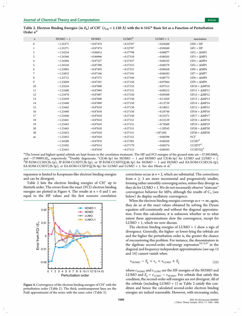
expansion is limited to Koopmans-like electron binding energiesand can be divergent.Table 2 lists the electron binding energies of CH+ up to

thirtieth order. The errors from the exact (FCI) electron bindingenergies are plotted in Figure 4. The results at n = 0 and 1 areequal to the HF values and the first nonzero correlation

corrections occur at n = 2, which are substantial. The correctionsfrom n ≥ 3 are more incremental and progressively smaller,forming rather smoothly converging series, unless they diverge asthey do for LUMO+ 1.We do not necessarily observe “staircase”convergence behavior for MPn, although the results of C2 (seebelow) do display oscillatory convergence.When the electron binding energies converge as n→∞, again,

they do so at the exact values obtained by solving the Dysonequation self-consistently and without the diagonal approxima-tion. From this calculation, it is unknown whether or to whatextent these approximations slow the convergence, except forLUMO + 1, which we now discuss.The electron binding energies of LUMO + 1 show a sign of

divergence. Generally, the higher- or lower-lying the orbitals areand the higher the perturbation order is, the greater the chanceof encountering this problem. For instance, the denominators inthe algebraic second-order self-energy expression10,13,47 in thediagonal and frequency-independent approximations (see eqs 13and 14) cannot vanish when

ϵ − < ϵ < ϵ +E Eg x gHOMO LUMO (33)

where ϵHOMO and ϵLUMO are the HF energies of the HOMO andLUMO and Eg = ϵLUMO − ϵHOMO. For orbitals that satisfy thiscondition, the second-order self-energies are not divergent. All ofthe orbitals (including LUMO + 1) in Table 2 satisfy this con-dition and hence the calculated second-order electron bindingenergies are indeed reasonable. However, with increasing order,

Table 2. Electron Binding Energies (in Eh) of CH+ (rCH = 1.120 Å) with the 6-31G* Basis Set as a Function of Perturbation

Order na

n HOMO − 1 HOMO LUMOb LUMO + 1 annotation

0 −1.25371 −0.87474 −0.32787 −0.04260 GF0 = HF1 −1.25371 −0.87474 −0.32787 −0.04260 GF1 = HF2 −1.24254 −0.86615 −0.37798 −0.06077 GF2 = ΔMP23 −1.24346 −0.86966 −0.37510 −0.06265 GF3 = ΔMP34 −1.24304 −0.87227 −0.37437 −0.06332 GF4 = ΔMP45 −1.24158 −0.87398 −0.37315 −0.06379 GF5 = ΔMP56 −1.23985 −0.87493 −0.37231 −0.06458 GF6 = ΔMP67 −1.23833 −0.87546 −0.37191 −0.06583 GF7 = ΔMP78 −1.23712 −0.87575 −0.37169 −0.06773 GF8 = ΔMP89 −1.23620 −0.87591 −0.37158 −0.07064 GF9 = ΔMP910 −1.23554 −0.87600 −0.37153 −0.07513 GF10 = ΔMP1011 −1.23508 −0.87604 −0.37151 −0.08213 GF11 = ΔMP1112 −1.23478 −0.87607 −0.37150 −0.09308 GF12 = ΔMP1213 −1.23459 −0.87608 −0.37150 −0.11029 GF13 = ΔMP1314 −1.23448 −0.87609 −0.37150 −0.13739 GF14 = ΔMP1415 −1.23442 −0.87610 −0.37150 −0.18011 GF15 = ΔMP1516 −1.23440 −0.87610 −0.37150 −0.24746 GF16 = ΔMP1617 −1.23440 −0.87610 −0.37150 −0.35371 GF17 = ΔMP1718 −1.23441 −0.87610 −0.37151 −0.52129 GF18 = ΔMP1819 −1.23443 −0.87610 −0.37151 −0.78560 GF19 = ΔMP1920 −1.23445 −0.87610 −0.37151 −1.20242 GF20 = ΔMP2030 −1.23453 −0.87610 −0.37151 −107.692 GF30 = ΔMP30∞ −1.23453 −0.87610 −0.37151 −0.06398 FCIc

−1.24588 −0.87876 −0.37301 −0.06250 CCSDd

−1.23505 −0.87614 −0.37179 −0.06374 CCSDTd

−1.23453 −0.87610 −0.37151 −0.06393 CCSDTQd

aThe lowest and highest spatial orbitals are kept frozen in the correlation treatment. The HF and FCI energies of the ground state are −37.895388Ehand −37.990913Eh, respectively. bDoubly degenerate. cCI(4h-3p) for HOMO − 1 and HOMO and CI(4h-5p) for LUMO and LUMO + 1.dIP-EOM-CCSD(2h-1p), IP-EOM-CCSDT(3h-2p), or IP-EOM-CCSDTQ(4h-3p) for HOMO − 1 and HOMO and EA-EOM-CCSD(1h-2p),EA-EOM-CCSDT(2h-3p), or EA-EOM-CCSDTQ(3h-4p) for LUMO and LUMO + 1. See also Hirata et al.7

Figure 4.Convergence of the electron binding energies of CH+ with theperturbation order (Table 2). The thick, semitransparent lines are thePade approximants of the series with the same color (Table 3).



1600


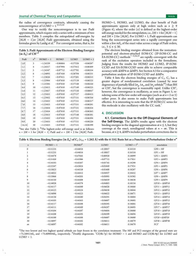
the radius of convergence contracts, ultimately causing thenonconvergence of LUMO + 1.43,55,56

One way to rectify the nonconvergence is to use Pade approximants, which require only a series with a minimum of twomembers. Table 3 compiles the extrapolated self-energies by[M,M − 1]or [M,M] Pade approximants, obtained using theformulas given by Laidig et al.57 For convergent series, that is, for

HOMO−1, HOMO, and LUMO, the clear benefit of Pade approximants appears only at high orders such as n ≥ 9(Figure 4), where the order (n) is defined as the highest-orderself-energy needed for the extrapolation, i.e., 2M + 1 for [M,M− 1]and 2M + 2 for [M,M]. For LUMO + 1, Pade approximants canbring the nonconvergent series into a rapidly convergent onewithin a few mEh of the exact value across a range of Pade orders,i.e., 3 ≤ n ≤ 30.The electron binding energies obtained from the ionization-

potential and electron-attached EOM-CC (IP-EOM-CC andEA-EOM-CC) methods7−9,58,59 are rapidly convergent with therank of the excitation operators included in the formalisms.Judging from the results for HOMO and LUMO, IP-EOM-CCSD and EA-EOM-CCSD seem able to achieve comparableaccuracy withΔMP4 orΔMP5. See Section 4.3 for a comparativeperturbation analysis of IP-EOM-CCSD and ΔMPn.Table 4 lists the electron binding energies of C2. C2 has a

greater degree of nondynamical correlation (caused by neardegeneracy of partially filled 2σg, 1πu, and 3σg orbitals

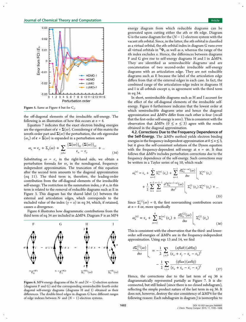
59) than BHor CH+, but the convergence is reasonably rapid. Unlike CH+,however, the convergence is oscillatory, as seen in Figure 5, re-ndering some of the low-order self-energies (such as at n = 2 or 3)rather poor. It also seems to make Pade approximants lesseffective. It is interesting to note that the IP-EOM-CC series forthis molecule is also oscillatory with the CC rank.7

4. DISCUSSION

4.1. Corrections Due to the Off-Diagonal Elements ofthe Self-Energy. The ΔMPn results agree with the electronbinding energies in the diagonal approximation at n≤ 3, but theyconverge at the exact, nondiagonal values at n = ∞. This isbecause, at n≥ 4,ΔMPn includes perturbation corrections due to

Table 3. Pade Approximants of the Electron Binding Energies(in Eh) of CH

+a

Pade nb HOMO − 1 HOMO LUMO LUMO + 1

[1,0] 3 −1.24339 −0.86864 −0.37526 −0.06287[1,1] 4 −1.24317 −0.87994 −0.37412 −0.06369[2,1] 5 −1.24347 −0.87712 −0.37701 −0.06554[2,2] 6 −1.24093 −0.87458 −0.36704 −0.06331[3,2] 7 −1.23626 −0.87611 −0.37201 −0.06253[3,3] 8 −1.22984 −0.87610 −0.37139 −0.06225[4,3] 9 −1.23385 −0.87610 −0.37148 −0.06226[4,4] 10 −1.23412 −0.87610 −0.37149 −0.06225[5,4] 11 −1.23457 −0.87610 −0.37150 −0.06057[5,5] 12 −1.23452 −0.87610 −0.37157 −0.06415[6,5] 13 −1.23452 −0.87610 −0.37151 −0.06356[6,6] 14 −1.23452 −0.87610 −0.37151 −0.06317[7,6] 15 −1.23453 −0.87610 −0.37151 −0.06281[7,7] 16 −1.23454 −0.87610 −0.37151 −0.06324[8,7] 17 −1.23454 −0.87610 −0.37151 −0.06363[8,8] 18 −1.23453 −0.87610 −0.37148 −0.06381[9,8] 19 −1.23452 −0.87610 −0.37151 −0.06394[9,9] 20 −1.23455 −0.87610 −0.37151 −0.06226[14,14] 30 −1.23453 −0.87610 −0.37151 −0.06399

aSee also Table 2. bThe highest-order self-energy used is as follows:n = 2M + 1 for [M,M − 1] Pade and n = 2M + 2 for [M,M] Pade.

Table 4. Electron Binding Energies (in Eh) of C2 (rCC = 1.262 Å) with the 6-31G Basis Set as a Function of Perturbation Order na

n HOMO − 1 HOMOb LUMO LUMO + 1b annotation

0 −0.51235 −0.44816 −0.10057 0.16318 GF0 = HF1 −0.51235 −0.44816 −0.10057 0.16318 GF1 = HF2 −0.54478 −0.47645 −0.06928 0.18099 GF2 = ΔMP23 −0.51450 −0.41986 −0.07715 0.17051 GF3 = ΔMP34 −0.54183 −0.45567 −0.05745 0.18290 GF4 = ΔMP45 −0.53347 −0.43824 −0.05849 0.17931 GF5 = ΔMP56 −0.53823 −0.44338 −0.05408 0.18287 GF6 = ΔMP67 −0.54022 −0.44412 −0.04937 0.18452 GF7 = ΔMP78 −0.53866 −0.44205 −0.05095 0.18382 GF8 = ΔMP89 −0.54150 −0.44508 −0.04659 0.18638 GF9 = ΔMP910 −0.54028 −0.44378 −0.04803 0.18534 GF10 = ΔMP1011 −0.54117 −0.44500 −0.04626 0.18666 GF11 = ΔMP1112 −0.54123 −0.44524 −0.04638 0.18644 GF12 = ΔMP1213 −0.54098 −0.44523 −0.04622 0.18671 GF13 = ΔMP1314 −0.54136 −0.44580 −0.04591 0.18684 GF14 = ΔMP1415 −0.54105 −0.44563 −0.04607 0.18685 GF15 = ΔMP1516 −0.54117 −0.44588 −0.04595 0.18685 GF16 = ΔMP1617 −0.54111 −0.44589 −0.04597 0.18695 GF17 = ΔMP1718 −0.54104 −0.44587 −0.04604 0.18680 GF18 = ΔMP1819 −0.54108 −0.44595 −0.04599 0.18694 GF19 = ΔMP1920 −0.54100 −0.44588 −0.04607 0.18680 GF20 =ΔMP2030 −0.54097 −0.44582 −0.04611 0.18679 GF30 = ΔMP30∞ −0.54097 −0.44582 −0.04611 0.18679 FCIc

aThe two lowest and two highest spatial orbitals are kept frozen in the correlation treatment. The HF and FCI energies of the ground state are−75.349114Eh and −75.609844Eh, respectively. bDoubly degenerate. cCI(8h-7p) for HOMO − 1 and HOMO and CI(8h-9p) for LUMO andLUMO + 1.



1601


the off-diagonal elements of the irreducible self-energy. Thefollowing is an illustration of how this occurs at n = 4.Equation 7 indicates that the exact electron binding energies

are the eigenvalues of ϵ + Σ(ω). Considering ϵ of this matrix thezeroth-order part and Σ(ω) the perturbation, the xth eigenvalue(ωx) of ϵ + Σ(ω) is expanded in a perturbation series

∑ω ωω ωΣ Σ

= ϵ + Σ +ϵ − ϵ

+≠

( ){ ( )} { ( )}

...x x xy x

xy yx

x y (34)

Substituting ω = ϵx in the right-hand side, we obtain aperturbation formula for ωx in the nondiagonal, frequency-independent approximation. The truncation of this equationafter the second term amounts to the diagonal approximation(eq 11). The third term is, therefore, the leading-ordercontribution from the off-diagonal elements of the irreducibleself-energy. The restriction in the summation index, y≠ x, in thisterm is related to the removal of reducible diagrams such as E inFigure 3. This diagram has the shared label (x) between theexternal and articulation edges, which corresponds to theexcluded value of the index (y = x) in eq 34, which, if retained,causes a divergence.Figure 6 illustrates how diagrammatic contributions from the

third term of eq 34 are included in ΔMP4. Diagram F is an MP4

energy diagram from which reducible diagrams can begenerated upon cutting either the ath or ith edge. DiagramG is the same diagram for the (N− 1)-electron system with thevacant xth orbital. Since, in the latter, the xth orbital is classifiedas a virtual orbital, the ath orbital index in diagram G runs overall virtual orbitals in NΦ0 as well as x, whereas the range of theith index excludes x. Hence, the differences between diagramsF and G give rise to self-energy diagrams H and I in ΔMP4.They are identified as semireducible diagrams and areconcatenation of two second-order irreducible self-energydiagrams with an articulation edge. They are not reduciblediagrams such as E because the label of the articulation edgediffers from that of the external edges in each case. In fact, thecombined range of the articulation-edge index in diagrams Hand I is all orbitals except x, in agreement with the third termin eq 34.In short, semireducible diagrams such as H and I account for

the effect of the off-diagonal elements of the irreducible self-energy. Figure 6 furthermore indicates that the lowest order atwhich semireducible diagrams arise and hence the diagonalapproximation and ΔMPn differ from each other is four (recallthat the first-order self-energy is zero). This is consistent with theobservation that ΔMPn (0 ≤ n ≤ 3) agree with the resultsobtained in the diagonal approximation.

4.2. Corrections Due to the Frequency Dependence ofthe Self-Energy. The ΔMPn method yields electron bindingenergies in the frequency-independent approximation at 0≤ n≤ 3,but it gives the self-consistent solutions of the Dyson equationwith the frequency-dependent self-energy at n = ∞. It thusfollows that ΔMPn includes perturbation corrections due to thefrequency dependence of the self-energy. Such corrections maybe written in a Taylor series of eq 10, which reads

∑ ∑

∑ ∑

ωω

ω

ωω

= ϵ + Σ ϵ +∂Σ

∂Σ ϵ

+∂ Σ

∂Σ ϵ Σ ϵ +

= =

− −

ϵ

=

−

=

− − − −

ϵ

( )( )

( )

12

( )( ) ( ) ...

xn

xm

n

xm

xm

nxn m

xm

x

l

n

m

n lxn l m

xl

x xm

x

( )

2

( )

1

1 ( )( )

1

2

1

1 2 ( )

2( ) ( )

x

x

(35)

Since Σx(1)(ω) = 0, the first nonvanishing contribution occurs

at n = 4 or, more specifically

∑ωω

ω= ϵ + Σ ϵ +

∂Σ∂

Σ ϵ= ϵ

( )( )

( )x xm

xm

xx

x x(4)

2

4( )

(2)(2)

x (36)

This is consistent with the observation that the third- and lower-order self-energies of ΔMPn are in the frequency-independentapproximation. Using eqs 13 and 14, we find

∑

∑

ωω

∂Σ∂

= −⟨ || ⟩⟨ || ⟩

ϵ + ϵ − ϵ − ϵ

−⟨ || ⟩⟨ || ⟩

ϵ + ϵ − ϵ − ϵ

ϵ

xj ab ab xj

ij ax ax ij

( ) 12 ( )

12 ( )

x

j a b x j a b

i j a x a i j

(2)

, ,2

, ,2

x

(37)

Hence, the corrections due to the last term of eq 36 isdiagrammatically represented partially as Figure 7. It is dis-connected, but still linked (since there is no closed subdiagram),reflecting the simple product nature of the last term in eq 36. Itdoes not, however, destroy the size consistency ofΔMP4 for thefollowing reason: Each subdiagram in diagram J is isomorphic to

Figure 5. Same as Figure 4 but for C2.

Figure 6.MP4 energy diagrams of theN- and (N − 1)-electron systems(diagrams F and G) and the corresponding semireducible fourth-orderdiagonal self-energy diagrams (diagrams H and I) obtained as theirdifferences. The double-lined edges in diagram G have different rangesof edge indexes between N- and (N − 1)-electron systems.



1602


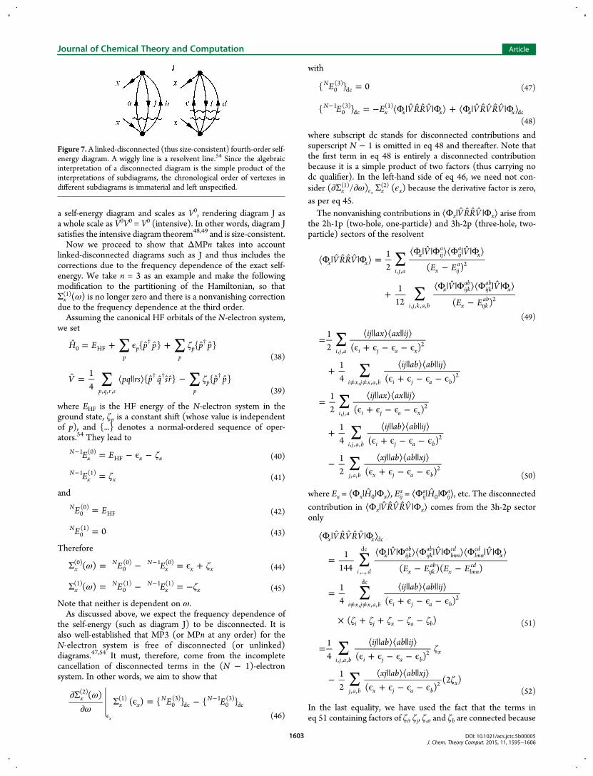
a self-energy diagram and scales as V0, rendering diagram J asa whole scale as V0V0 = V0 (intensive). In other words, diagram Jsatisfies the intensive diagram theorem48,49 and is size-consistent.Now we proceed to show that ΔMPn takes into account

linked-disconnected diagrams such as J and thus includes thecorrections due to the frequency dependence of the exact self-energy. We take n = 3 as an example and make the followingmodification to the partitioning of the Hamiltonian, so thatΣx(1)(ω) is no longer zero and there is a nonvanishing correction

due to the frequency dependence at the third order.Assuming the canonical HF orbitals of the N-electron system,

we set

∑ ∑ ζ = + ϵ + † †H E p p p p{ } { }p

pp

p0 HF(38)

∑ ∑ ζ = ⟨ || ⟩ − † † †V pq rs p q sr p p14

{ } { }p q r s p

p, , , (39)

where EHF is the HF energy of the N-electron system in theground state, ζp is a constant shift (whose value is independentof p), and {...} denotes a normal-ordered sequence of oper-ators.54 They lead to

ζ= − ϵ −− E ENx x x

1 (0)HF (40)

ζ=− ENx x

1 (1)(41)

and

=E EN0(0)

HF (42)

=E 0N0(1)

(43)

Therefore

ω ζΣ = − = ϵ +−E E( )xN N

x x x(0)

0(0) 1 (0)

(44)

ω ζΣ = − = −−E E( )xN N

x x(1)

0(1) 1 (1)

(45)

Note that neither is dependent on ω.As discussed above, we expect the frequency dependence of

the self-energy (such as diagram J) to be disconnected. It isalso well-established that MP3 (or MPn at any order) for theN-electron system is free of disconnected (or unlinked)diagrams.47,54 It must, therefore, come from the incompletecancellation of disconnected terms in the (N − 1)-electronsystem. In other words, we aim to show that

ωω

∂Σ∂

Σ ϵ = −ϵ

−E E( )

( ) { } { }xx x

N N(2)

(1)0(3)

dc1

0(3)

dc

x (46)

with

=E{ } 0N0(3)

dc (47)

= − ⟨Φ | |Φ ⟩ + ⟨Φ | |Φ ⟩− E E VRRV VRVRV{ }Nx x x x x

10(3)

dc(1)

dc(48)

where subscript dc stands for disconnected contributions andsuperscript N − 1 is omitted in eq 48 and thereafter. Note thatthe first term in eq 48 is entirely a disconnected contributionbecause it is a simple product of two factors (thus carrying nodc qualifier). In the left-hand side of eq 46, we need not con-sider (∂Σx

(1)/∂ω)ϵx Σx(2) (ϵx) because the derivative factor is zero,

as per eq 45.The nonvanishing contributions in ⟨Φx| VRRV |Φx⟩ arise from

the 2h-1p (two-hole, one-particle) and 3h-2p (three-hole, two-particle) sectors of the resolvent

∑

∑

⟨Φ | |Φ ⟩ =⟨Φ | |Φ ⟩⟨Φ | |Φ ⟩

−

+⟨Φ | |Φ ⟩⟨Φ | |Φ ⟩

−

VRRVV V

E E

V V

E E

12 ( )

112 ( )

x xi j a

x ija

ija

x

x ija

i j k a b

x ijkab

ijkab

x

x ijkab

, ,2

, , , ,2

(49)

∑

∑

∑

∑

∑

=⟨ || ⟩⟨ || ⟩

ϵ + ϵ − ϵ − ϵ

+⟨ || ⟩⟨ || ⟩

ϵ + ϵ − ϵ − ϵ

=⟨ || ⟩⟨ || ⟩

ϵ + ϵ − ϵ − ϵ

+⟨ || ⟩⟨ || ⟩

ϵ + ϵ − ϵ − ϵ

−⟨ || ⟩⟨ || ⟩

ϵ + ϵ − ϵ − ϵ

≠ ≠

ij ax ax ij

ij ab ab ij

ij ax ax ij

ij ab ab ij

xj ab ab xj

12 ( )

14 ( )

12 ( )

14 ( )

12 ( )

i j a i j a x

i x j x a b i j a b

i j a i j a x

i j a b i j a b

j a b x j a b

, ,2

, , ,2

, ,2

, , ,2

, ,2

(50)

where Ex = ⟨Φx|H0|Φx⟩, Eija = ⟨Φij

a|H0|Φija⟩, etc. The disconnected

contribution in ⟨Φx| VRVRV |Φx⟩ comes from the 3h-2p sectoronly

∑

∑

ζ ζ ζ ζ ζ

⟨Φ | |Φ ⟩

=⟨Φ | |Φ ⟩⟨Φ | |Φ ⟩⟨Φ | |Φ ⟩

− −

=⟨ || ⟩⟨ || ⟩

ϵ + ϵ − ϵ − ϵ

× + + − −

≠ ≠

VRVRV

V V V

E E E E

ij ab ab ij

1144 ( )( )

14 ( )

( )

x x

i d

x ijkab

ijkab

lmncd

lmncd

x

x ijkab

x lmncd

i x j x a b i j a b

i j x a b

dc

,...,

dc

, , ,

dc

2

(51)

∑

∑

ζ

ζ

=⟨ || ⟩⟨ || ⟩

ϵ + ϵ − ϵ − ϵ

−⟨ || ⟩⟨ || ⟩

ϵ + ϵ − ϵ − ϵ

ij ab ab ij

xj ab ab xj

14 ( )

12 ( )

(2 )

i j a b i j a bx

j a b x j a bx

, , ,2

, ,2

(52)

In the last equality, we have used the fact that the terms ineq 51 containing factors of ζi, ζj, ζa, and ζb are connected because

Figure 7.A linked-disconnected (thus size-consistent) fourth-order self-energy diagram. A wiggly line is a resolvent line.54 Since the algebraicinterpretation of a disconnected diagram is the simple product of theinterpretations of subdiagrams, the chronological order of vertexes indifferent subdiagrams is immaterial and left unspecified.



1603


i, j, a, and b are among the summation indexes, whereas the termcontaining ζx is disconnected.Substituting eqs 50 and 52 into eq 48, we obtain

∑

∑

ζ

ζ

⟨Φ | |Φ ⟩ − ⟨Φ | |Φ ⟩

= −⟨ || ⟩⟨ || ⟩

ϵ + ϵ − ϵ − ϵ−

−⟨ || ⟩⟨ || ⟩

ϵ + ϵ − ϵ − ϵ−

E VRRV VRVRVij ax ax ij

xj ab ab xj

12 ( )

( )

12 ( )

( )

x x x x x

i j a i j a xx

j a b x j a bx

(1)dc

, ,2

, ,2

(53)

which is found to be equal to the left-hand side of eq 46.Essentially the same proof can be constructed for ΔMP3between the (N + 1)- and N-electron systems.We have shown that ΔMP3 (with a modified partitioning of

the Hamiltonian) contains the third-order correction due to thefrequency dependence of the exact self-energy in the formof eq 35. We conjecture that this holds true at higher orders andwith theMøller−Plesset partitioning of the Hamiltonian, makingΔMPn converge at the exact, self-consistent solutions of theDyson equation as n → ∞.4.3. Relationship to EOM-CC. The diagrammatic corre-

spondence between the CC and MP methods for the groundstate is well-established.54,60 Since the IP- and EA-EOM-CCmethods with the N-electron HF reference wave function yieldconverging results for electron binding energies, they shouldaccount for all diagrammatic contributions in ΔMPn. Here, weshow that self-energy diagrams B and C (Figure 1) as well assemireducible diagrams H and I (Figure 6) and linked-disconnected diagram J (Figure 7) ofΔMPn are indeed includedin IP-EOM-CCSD in the case of electron-detachment energies.The CI-like eigenvalue equations of IP-EOM-CCSD can be

written as

∑ ∑ω− = −ϵ − ⟨ || ⟩ − ⟨ || ⟩ +r r ij ak r ij ab t r12

12

...k k ki j a

ija

i j a bikab

j, , , , ,

(54)

∑ω− = −ϵ − ϵ + ϵ − ⟨ || ⟩ +r r ak ij r( ) ...ija

i j a ija

kk

(55)

where only relevant terms are shown and the eigenvalue(electron-detachment energy),ω, is multiplied by−1 to facilitatethe correspondence withΔMPn. Here, tij

ab is the amplitude of thecluster excitation operator, which is known from the precedingCCSD calculation, and rk and rij

a are the amplitudes of the 1h and2h-1p ionization operators to be determined by solving theseequations.The zeroth-order perturbation approximations to ω and rk

for the Koopmans-like final state in which the xth orbital isvacant are

Σ = ϵx x(0)

(56)

δ=rk kx(0)

(57)

Substituting these into eq 55 truncated after the second termyields the first-order approximation to rij

a as

=⟨ || ⟩

ϵ + ϵ − ϵ − ϵr

ax ijija

x a i j

(1)

(58)

The corresponding approximation to tijab is the MP1 excitation

amplitude

=⟨ || ⟩

ϵ + ϵ − ϵ − ϵt

ab ijijab

i j a b

(1)

(59)

Substituting these into eq 54 gives the second-order correction toω, which reads

∑ ∑

∑

∑

Σ = ⟨ || ⟩ + ⟨ || ⟩

=⟨ || ⟩⟨ || ⟩

ϵ + ϵ − ϵ − ϵ

+ ⟨ || ⟩⟨ || ⟩ϵ + ϵ − ϵ − ϵ

ij ax r ij ab t r

ij ax ax ij

ab ix ix ab

12

12

12

12

xi j a

ija

i j a bixab

j

i j a x a i j

i a b x i a b

(2)

, ,

(1)

, , ,

(1) (0)

, ,

, , (60)

which agrees exactly with the sum of eqs 13 and 14 at ω = ϵx(diagrams B and C). Here, we define the perturbation order bythe number of appearances of the fluctuation potential in eachterm.A part of the second-order correction to rk can be obtained by

substituting eqs 56−58 into eq 54 truncated after the secondterm, yielding

∑

∑

= Σ − ϵ ⟨ || ⟩

=⟨ || ⟩⟨ || ⟩

ϵ + ϵ − ϵ − ϵ ϵ − ϵ

≠−r ij ak r

ax ij ij ak

{ }12

12 ( )( )

k x x ki j a

ija

i j a x a i j x k

(2) (0) 1

, ,

(1)

, , (61)

Note that this expression is valid only for k ≠ x, lest it diverges.This in conjunction with eq 55 truncated after the second termsuggests the third-order correction to rij

a as

∑

∑ ∑

= Σ + ϵ − ϵ − ϵ ⟨ || ⟩

=⟨ || ⟩⟨ || ⟩⟨ || ⟩

ϵ + ϵ − ϵ − ϵ ϵ − ϵ ϵ + ϵ − ϵ − ϵ

−≠

≠

r ak ij r

bx lm lm bk ak ij

{ }

12 ( )( )( )

ija

x a i jk

k x

l m b k x x b l m x k x a i j

(3a) (0) 1 (2)

, ,

(62)

Its substitution into the second term in the right-hand sideof eq 54 leads to a fourth-order correction to ω

∑

∑ ∑ ∑

Σ = ⟨ || ⟩

=⟨ || ⟩⟨ || ⟩⟨ || ⟩⟨ || ⟩

ϵ + ϵ − ϵ − ϵ ϵ − ϵ ϵ + ϵ − ϵ − ϵ≠

ij ax r

bx lm lm bk ak ij ij ax

12

14 ( )( )( )

xi j a

ija

i j a l m b k x x b l m x k x a i j

(4a)

, ,

(3a)

, , , ,

(63)

which is exactly the contribution from semireducible diagramH at ω = ϵx, accounting for the off-diagonal elements of theirreducible self-energy (diagram C). The index restriction, k ≠ x,distinguishes this term from reducible diagram E.Another third-order correction to rij

a can be obtained byadopting the second-order approximation for ω in eq 55truncated after the second term

∑+ = Σ + Σ + ϵ − ϵ − ϵ ⟨ || ⟩

≈⟨ || ⟩

ϵ + ϵ − ϵ − ϵ−

Σ ⟨ || ⟩ϵ + ϵ − ϵ − ϵ

−r r ak ij r

ax ij ax ij

{ }

( )

ija

ija

x x a i jk

k

x a i j

x

x a i j

(1) (3b) (2) (0) 1 (0)

(2)

2

(64)

In the second equality, a use is made of the Maclaurin series:(1 + δ)−1 ≈ 1 − δ, with δ = (2)Σx/(ϵx + ϵa − ϵi − ϵj). Substitutionof the third-order correction into eq 54 gives a fourth-ordercorrection to ω in the form



1604


∑

∑

Σ = ⟨ || ⟩

= −⟨ || ⟩⟨ || ⟩

ϵ + ϵ − ϵ − ϵΣ

ij ax r

ax ij ij ax

12

12 ( )

xi j a

ija

i j a x a i jx

(4b)

, ,

(3b)

, ,2

(2)

(65)

which accounts for two of the linked-disconnected diagramcontributions in the last term of eq 36 analogous to diagram J.Nooijen and Snijders pointed out61,62 that IP- and EA-EOM-CC

can be viewed as a GF theory.

5. CONCLUSIONS

An nth-order self-energy can be defined as the difference in MPnenergy between the N- and (N ± 1)-electron systems (ΔMPn),which are, in turn, evaluated by the determinant-based, general-order MPn method1 at any n. This constitutes a general-orderimplementation of a one-electron GF method.The electron binding energies calculated with ΔMPn (n ≤ 3)

agree identically with the solutions of the Dyson equation in thediagonal and frequency-independent approximations to the self-energy. However, the converged limits of the binding energies atn =∞ (if they do converge) are the exact basis-set values, that is,the solutions of the Dyson equation with the exact, nondiagonal,frequency-dependent self-energy. This suggests that the electronbinding energies of ΔMPn include perturbation correctionsdue to the off-diagonal elements and frequency dependence ofthe self-energy, which may be zero at n ≤ 3 but are nonzero else-where. Therefore,ΔMPn defines a new, converging expansion ofthe exact self-energies for Koopmans-like transitions, whosecomputer implementation does not involve diagonalizationor self-consistent solutions of a recursive equation. Our dia-grammatic analysis shows that these corrections are accountedfor by semireducible and linked-disconnected diagrams. Thelowest order at which these diagrams appear is four and thesefourth-order diagrams are also included in IP- or EA-EOM-CCSD.In CH+, the electron binding energies of ΔMPn display

smooth, nearly monotonic convergence at n > 2, unless theydisplay a sign of divergence. Pade approximants are shown toextrapolate the correct limit within a few mEh from theseapparently divergent series. In C2, the electron binding energiesof the four frontier orbitals are oscillatory but convergent. Theapproximations defined by ΔMPn are, therefore, expected tobe useful up to high orders and especially so when combinedwith Pade approximants in the case of divergent series. Eachdiagrammatic contribution of ΔMPn can be recast into a singlehigh-dimensional integral and subject to a highly scalable MonteCarlo evaluation,63 owing to the aforementioned inherentalgorithmic simplicity.

■ AUTHOR INFORMATION

Corresponding Author*E-mail: [email protected].

FundingThis work was supported by the SciDAC program of the U.S.Department of Energy, Office of Science, Basic Energy Sciences,under award no. DE-FG02-12ER46875 and CREST, JapanScience and Technology Agency.

NotesThe authors declare no competing financial interest.

■ ACKNOWLEDGMENTS

S.H. is a Camille Dreyfus Teacher-Scholar and a Scialog Fellow ofthe Research Corporation for Science Advancement.

■ REFERENCES(1) Knowles, P. J.; Somasundram, K.; Handy, N. C.; Hirao, K. Chem.Phys. Lett. 1985, 113, 8−12.(2) Knowles, P. J.; Handy, N. C. Chem. Phys. Lett. 1984, 111, 315−321.(3) Hirata, S.; Bartlett, R. J. Chem. Phys. Lett. 2000, 321, 216−224.(4) Kallay, M.; Surjan, P. R. J. Chem. Phys. 2000, 113, 1359−1365.(5) Olsen, J. J. Chem. Phys. 2000, 113, 7140−7148.(6) Hirata, S.; Nooijen, M.; Bartlett, R. J. Chem. Phys. Lett. 2000, 326,255−262.(7) Hirata, S.; Nooijen, M.; Bartlett, R. J. Chem. Phys. Lett. 2000, 328,459−468.(8) Stanton, J. F.; Bartlett, R. J. J. Chem. Phys. 1993, 98, 7029−7039.(9) Nooijen, M.; Bartlett, R. J. J. Chem. Phys. 1995, 102, 3629−3647.(10) Linderberg, J.; Ohrn, Y. Propagators in Quantum Chemistry;Academic Press: London, 1973.(11) Cederbaum, L. S.; Domcke, W. Adv. Chem. Phys. 1977, 36, 205−344.(12) Simons, J. Annu. Rev. Phys. Chem. 1977, 28, 15−45.(13) Jørgensen, P.; Simons, J. Second Quantization-Based Methods inQuantum Chemistry; Academic Press: New York, 1981.(14) Ohrn, Y.; Born, G. Adv. Quantum Chem. 1981, 13, 1−88.(15) Herman, M. F.; Freed, K. F.; Yeager, D. L. Adv. Chem. Phys. 1981,48, 1−69.(16) von Niessen, W.; Schirmer, J.; Cederbaum, L. S. Comput. Phys.Rep. 1984, 1, 57−125.(17) Oddershede, J. Adv. Chem. Phys. 1987, 69, 201−239.(18) Ortiz, J. V. Adv. Quantum Chem. 1999, 35, 33−52.(19) Danovich, D. Wiley Interdiscip. Rev.: Comput. Mol. Sci. 2011, 1,377−387.(20) Suhai, S. Phys. Rev. B 1983, 27, 3506−3518.(21) Sun, J.-Q.; Bartlett, R. J. Phys. Rev. Lett. 1996, 77, 3669−3672.(22) Hirata, S.; Shimazaki, T. Phys. Rev. B 2009, 80, 085118.(23) Willow, S. Y.; Kim, K. S.; Hirata, S. Phys. Rev. B 2014, 90,201110(R).(24) Onida, G.; Reining, L.; Rubio, A. Rev. Mod. Phys. 2002, 74, 601−659.(25) Pickup, B. T.; Goscinski, O. Mol. Phys. 1973, 26, 1013−1035.(26) Mattuck, R. D. A Guide to Feynman Diagrams in the Many-BodyProblem; Dover: New York, 1992.(27) March, N. H.; Young, W. H.; Sampanthar, S. The Many-BodyProblem in Quantum Mechanics; Cambridge University Press: Cam-bridge, 1967.(28) Cederbaum, L. S.; Hohlneicher, G.; Niessen, W. Chem. Phys. Lett.1973, 18, 503−508.(29) Simons, J.; Smith, W. D. J. Chem. Phys. 1973, 58, 4899−4907.(30) Redmon, L. T.; Purvis, G.; Ohrn, Y. J. Chem. Phys. 1975, 63,5011−5017.(31) Purvis, G. D.; Ohrn, Y. Chem. Phys. Lett. 1975, 33, 396−398.(32) Jørgensen, P.; Simons, J. J. Chem. Phys. 1975, 63, 5302−5304.(33) Herman, M. F.; Yeager, D. L.; Freed, K. F. Chem. Phys. 1978, 29,77−96.(34) Zakrzewski, V. G.; Ortiz, J. V. Int. J. Quantum Chem. 1995, 53,583−590.(35) Ortiz, J. V. J. Chem. Phys. 1996, 104, 7599−7605.(36) Ortiz, J. V.; Zakrzewski, V. G. J. Chem. Phys. 1996, 105, 2762−2769.(37) Ortiz, J. V. Int. J. Quantum Chem. 1997, 63, 291−299.(38) Ortiz, J. V. J. Chem. Phys. 1998, 108, 1008−1014.(39) Ferreira, A. M.; Seabra, G.; Dolgounitcheva, O.; Zakrzewski, V.G.; Ortiz, J. V. In Quantum-Mechanical Prediction of ThermochemicalData; Cioslowski, J., Ed.; Kluwer Academic Publishers: Boston, MA,2001; pp 131−160.(40) Schirmer, J.; Cederbaum, L. S.; Walter, O. Phys. Rev. A 1983, 28,1237−1259.



1605

mailto:[email protected]


(41) Ortiz, J. V. J. Chem. Phys. 1988, 89, 6348−6352.(42) Ortiz, J. V. J. Chem. Phys. 1988, 89, 6353−6356.(43) Nobes, R. H.; Pople, J. A.; Radom, L.; Handy, N. C.; Knowles, P. J.Chem. Phys. Lett. 1987, 138, 481−485.(44) Chong, D. P.; Herring, F. G.; McWilliams, D. J. Chem. Phys. 1974,61, 78−84.(45) Chong, D. P.; Herring, F. G.; McWilliams, D. J. Chem. Phys. 1974,61, 958−962.(46) Chong, D. P.; Herring, F. G.; McWilliams, D. J. Chem. Phys. 1974,61, 3567−3570.(47) Szabo, A.; Ostlund, N. S.Modern Quantum Chemistry; MacMillan:New York, 1982.(48) Hirata, S. Theor. Chem. Acc. 2011, 129, 727−746.(49) Hirata, S.; Keceli, M.; Ohnishi, Y.; Sode, O.; Yagi, K. Annu. Rev.Phys. Chem. 2012, 63, 131−153.(50) Hermes, M. R.; Hirata, S. J. Chem. Phys. 2013, 139, 034111.(51) Bloch, C.; De Dominicis, C. Nucl. Phys. 1958, 7, 459−479.(52) Bloch, C. In Studies in Statistical Mechanics; De Boer, J.,Uhlenbeck, G. E., Eds.; North-Holland: Amsterdam, 1965; pp 3−211.(53) Hirata, S.; He, X.; Hermes, M. R.; Willow, S. Y. J. Phys. Chem. A2014, 118, 655−672.(54) Shavitt, I., Bartlett, R. J. Many-Body Methods in Chemistry andPhysics; Cambridge University Press: Cambridge, 2009.(55) Olsen, J.; Christiansen, O.; Koch, H.; Jørgensen, P. J. Chem. Phys.1996, 105, 5082−5090.(56) Sergeev, A. V.; Goodson, D. Z.; Wheeler, S. E.; Allen, W. D. J.Chem. Phys. 2005, 123, 064105.(57) Laidig, W. D.; Fitzgerald, G.; Bartlett, R. J. Chem. Phys. Lett. 1985,113, 151−158.(58) Kamiya, M.; Hirata, S. J. Chem. Phys. 2006, 125, 074111.(59) Kamiya, M.; Hirata, S. J. Chem. Phys. 2007, 126, 134112.(60) Bartlett, R. J. Annu. Rev. Phys. Chem. 1981, 32, 359−401.(61) Nooijen, M.; Snijders, J. G. Int. J. Quantum Chem. 1992, S26, 55−83.(62) Nooijen, M.; Snijders, J. G. Int. J. Quantum Chem. 1993, 48, 15−48.(63) Willow, S. Y.; Kim, K. S.; Hirata, S. J. Chem. Phys. 2013, 138,164111.



1606


Documents

General-Order Many-Body Green s Function Method