Generalized Quantile Treatment Effect: A Flexible … · A Flexible Bayesian Approach Using Quantile Ratio Smoothing Sergio Venturini ... S.Venturini,F.DominiciandG.Parmigiani 525

arX

iv:1

509.

0104

2v1

[m

ath.

ST]

3 S

ep 2

015

Bayesian Analysis (2015) 10, Number 3, pp. 523–552

Generalized Quantile Treatment Effect:

A Flexible Bayesian Approach Using Quantile

Ratio Smoothing

Sergio Venturini∗, Francesca Dominici†, and Giovanni Parmigiani‡

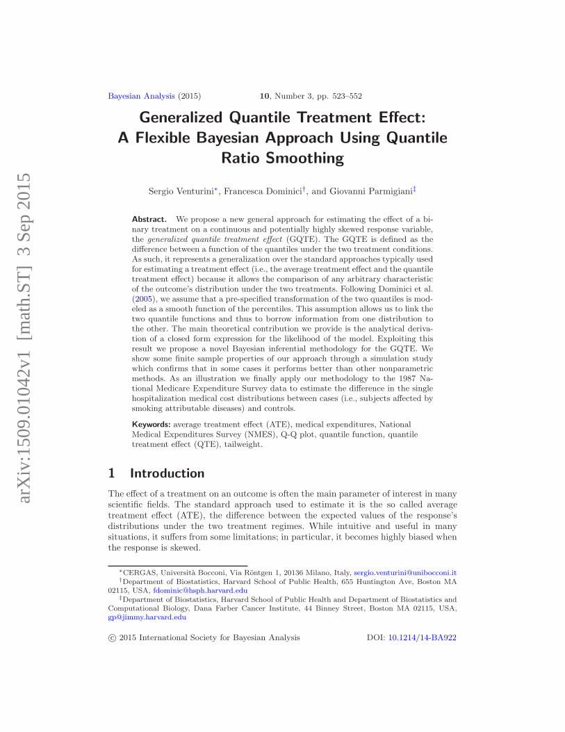
Abstract. We propose a new general approach for estimating the effect of a bi-nary treatment on a continuous and potentially highly skewed response variable,the generalized quantile treatment effect (GQTE). The GQTE is defined as thedifference between a function of the quantiles under the two treatment conditions.As such, it represents a generalization over the standard approaches typically usedfor estimating a treatment effect (i.e., the average treatment effect and the quantiletreatment effect) because it allows the comparison of any arbitrary characteristicof the outcome’s distribution under the two treatments. Following Dominici et al.(2005), we assume that a pre-specified transformation of the two quantiles is mod-eled as a smooth function of the percentiles. This assumption allows us to link thetwo quantile functions and thus to borrow information from one distribution tothe other. The main theoretical contribution we provide is the analytical deriva-tion of a closed form expression for the likelihood of the model. Exploiting thisresult we propose a novel Bayesian inferential methodology for the GQTE. Weshow some finite sample properties of our approach through a simulation studywhich confirms that in some cases it performs better than other nonparametricmethods. As an illustration we finally apply our methodology to the 1987 Na-tional Medicare Expenditure Survey data to estimate the difference in the singlehospitalization medical cost distributions between cases (i.e., subjects affected bysmoking attributable diseases) and controls.

Keywords: average treatment effect (ATE), medical expenditures, NationalMedical Expenditures Survey (NMES), Q-Q plot, quantile function, quantiletreatment effect (QTE), tailweight.

1 Introduction

The effect of a treatment on an outcome is often the main parameter of interest in manyscientific fields. The standard approach used to estimate it is the so called averagetreatment effect (ATE), the difference between the expected values of the response’sdistributions under the two treatment regimes. While intuitive and useful in manysituations, it suffers from some limitations; in particular, it becomes highly biased whenthe response is skewed.

∗CERGAS, Universita Bocconi, Via Rontgen 1, 20136 Milano, Italy, [email protected]†Department of Biostatistics, Harvard School of Public Health, 655 Huntington Ave, Boston MA

02115, USA, [email protected]‡Department of Biostatistics, Harvard School of Public Health and Department of Biostatistics and

Computational Biology, Dana Farber Cancer Institute, 44 Binney Street, Boston MA 02115, USA,[email protected]

c© 2015 International Society for Bayesian Analysis DOI: 10.1214/14-BA922

http://arxiv.org/abs/1509.01042v1

http://bayesian.org

mailto:[email protected]



http://dx.doi.org/10.1214/14-BA922

524 Generalized Quantile Treatment Effect

A further drawback of the ATE is its coarseness as a summary of the distancebetween the expected value of the response’s distributions under the two treatments. Itis a matter of fact indeed that the effect of the treatment on the outcome often varies aswe move from the lower to the upper tail of the outcome’s distribution. This limitationof the ATE has been addressed in the literature by introducing the so called quantiletreatment effect (QTE), the difference between the response’s distribution quantilesunder the two treatments (Abadie et al., 2002; Chernozhukov and Hansen, 2005; Firpo,2007; Frolich and Melly, 2008).

In this paper we propose a more general measure of the effect of a binary treatmenton a continuous outcome. We call it the generalized quantile treatment effect (GQTE),defined as

∆g(p) = g(Q1(p))− g(Q2(p)), (1)

where Q1(p) and Q2(p) represent the quantile functions of the outcome under the twotreatment conditions and g(·) is an arbitrary but known function of the quantiles. Forexample, if g(·) is chosen to be the identity function, then the GQTE simplifies to theQTE, while if g(·) is the integral over the percentile p, the GQTE becomes equivalentto the ATE. The GQTE is a new parameter which generalizes the existing approachesfor estimating a treatment effect.

To estimate and formulate inferences about the GQTE we propose a Bayesian ap-proach that can accommodate both symmetric and skewed outcomes, as well as situa-tions where the sample size under a treatment condition (cases) is much smaller thanthe sample size under the other treatment condition (controls). In particular, we assume

h

(Q1(p)

Q2(p)

)= s(p) , (2)

where h is a monotone function and s is assumed to be smooth. In other words, weassume that the transformed quantile ratio is a smooth function of the percentile p.The idea of smoothly modeling the ratio of the quantiles has been first introduced byDominici et al. (2005), who exploited it by proposing a nonparametric estimator ofthe mean difference between two populations. Here we generalize their approach bypermitting the comparison of any characteristic of the outcome’s distributions underthe two treatments.

An important theoretical contribution of this paper is the derivation of a closed formexpression for the model likelihood. We show that it is possible to obtain an analyticallytractable form for the Y2 density (the controls) without explicitly specifying a model forit. Clearly the likelihood is needed to carry out the Bayesian estimation but in principleit could be employed for classic likelihood procedures as well. Moreover, our proposedapproach allows one to borrow strength from one sample to the other, thus improvingefficiency in the estimation of the quantiles (Dominici et al., 2005).

As an illustration, we apply our method to the comparison of the single hospitaliza-tion medical costs distribution between subjects with and without smoking attributablediseases. The data set we use is the National Medical Expenditures Survey (NMES)supplemented by the Adult Self-Administered Questionnaire Household Survey.

S. Venturini, F. Dominici and G. Parmigiani 525

The paper is organized as follows. In Section 2 we define the new parameter ∆g(p)and illustrate some quantile-based measures that will be used in the paper. In Section 3we provide details of the estimation approach together with some special cases. Wethen present the results of a simulation study in Section 4 through which we concludethat under a broad set of conditions our approach performs better than other flexiblemethods for comparing two distributions. In Section 5 we illustrate the results of thedata analysis on the NMES data set. Section 6 concludes the paper with a discussionand some final remarks.

2 The Generalized Quantile Treatment Effect (GQTE)

Consider two positive continuous random variables Y1 and Y2 with quantile functionsQ1 and Q2, where

Qℓ(p) ≡ F−1ℓ (p) ≡ inf{y : Fℓ(y) ≥ p}

for 0 < p < 1 and ℓ = 1, 2. To compare F1 and F2 as flexibly as possible we introducethe generalized quantile treatment effect, which is defined as

∆g(p) = g(Q1(p))− g(Q2(p)), (3)

where g(·) is a known function of the quantiles. Notice that no a priori assumptions aremade about the admissible functions g(·), thus potentially any function of the quan-tiles can be used. Therefore, the GQTE provides a general approach to compare theresponse’s distributions under the two treatments. More precisely, by properly choosingthe function g(·), we can recover any specific characteristic of the outcome’s distributionsF1 and F2 and, through (3), their difference.

The simplest case arises when g(x) = x. In this case the GQTE simplifies to

∆(p) = Q1(p)−Q2(p), (4)

the so called (unconditional) QTE (Frolich and Melly, 2008), sometimes also namedthe percentile-specific effect between two populations (see for example Dominici et al.,2006, 2007).

A second example is obtained by choosing g(x) =∫x dp, which produces

∆ =

∫ 1

0

Q1(p) dp−∫ 1

0

Q2(p) dp , (5)

the extensively used ATE (see for example Wooldridge, 2010, Chapter 21).

These examples illustrate how the GQTE reduces to the two most used parametersof interest for estimating a treatment effect, the ATE and QTE. However, the GQTEcan provide a variety of other useful measures. In Appendix 1 we illustrate some otherinteresting cases that usually are not taken into consideration in the literature.


3 Estimation Methodology

In this section we illustrate the procedure we developed for estimating the GQTE. Ourproposed approach is sufficiently general that it can be used for any choice of g(·).

3.1 Definitions and Model Assumptions

We assume that Y1|η ∼ F1(· ;η), where F1 is a given probability distribution dependingupon a vector of unknown parameters η. For example, in the application presentedin Section 5 we choose F1 as a mixture distribution. To borrow information from onedistribution to the other, we assume that the transformed quantile ratio is a smoothfunction of the percentiles with λ degrees of freedom, that is

h

(Q1(p)

Q2(p)

)= s(p, λ) , 0 < p < 1 . (6)

The function h(·) is assumed to be monotone differentiable. It represents a kind oflink function and it is used to transform the quantile ratio to account for the potentialskewness of the F1 and F2. The typical choice for skewed data is h(x) = log x, while forsymmetric data distributions the identity function is the most reasonable option.

For the sake of simplicity, we henceforth indicate the smooth function s(p, λ) withreference to the corresponding design matrix X(p, λ), so that it can be written asX(p, λ)β, where β is a vector of unknown parameters. More explicitly, we assume that

s(p, λ) ≡ X(p, λ)β =∑λ

k=0 Xk(p)βk, where Xk(p) are orthonormal basis functions withX0(p) = 1. The number of degrees of freedom λ is a further parameter that has either tobe chosen or estimated from the data. In Subsection 3.7 we propose a simple approachfor eliciting it. The basis functions are usually either splines or polynomials.

The main justification for assuming (6) is that it allows one to borrow informationfrom both the response’s distributions under the two treatment conditions when weestimate the GQTE ∆g(p). Assumption (6), in fact, implies

Q1(p) = Q2(p)h−1 [X(p, λ)β] , (7)

and alsoQ2(p) = Q1(p)

{h−1 [X(p, λ)β]

}−1, (8)

which, once substituted in (3), return

∆g(p) = g(Q2(p)h

−1 [X(p, λ)β])− g(Q1(p)

{h−1 [X(p, λ)β]

}−1).

For the special case where g(x) = x and h(x) = log(x), Dominici et al. (2005) haveshown that under assumption (6) it is possible to obtain a more efficient estimator of ∆than the sample mean difference and the maximum likelihood estimator assuming thatY1 and Y2 are both log-normal.

Notice that, since the main interest in the paper resides in the estimation of ∆g(p),for which only β is required, η is treated as nuisance (see Subsection 3.6 for furtherdetails).


In this paper we propose a Bayesian approach for estimating ∆g(p) for any choice ofg(·) and h(·). An interesting feature of our estimation procedure for ∆g(p), is that weonly need to specify the distribution function for Y1. The specification of F1 togetherwith the relationship (6) automatically determines a distributional assumption for Y2.We refer to the distribution of Y2 induced by F1 and assumption (6) as F2(· ;β,η).

As a last remark for this section, we want to highlight the difference between thefunction g(·), introduced in the previous section, and h(·), defined above in (6). Theyshould not be confused because they have distinct roles: the former identifies the re-sponse’s characteristic we want to estimate for assessing the treatment effect, while thelatter has been introduced as a mechanism to attenuate the possible skewness presentin the data.

3.2 Estimation Approach and Likelihood

The steps involved in our estimation approach are summarized as follows:

1. Choose a (possibly flexible) density f1(y1|η) for Y1, a smoothing function s(p, λ)(usually a spline or a polynomial) and a value for λ;

2. From (8) derive the density function of Y2, that we denote as f2(y2|β,η). Notethat, as proved by Theorem 1 below, this density will depend on the model pa-rameter β as well as on the parameter η through the Y1 density.

3. Calculate the joint likelihood L (β,η|y1,y2) to use for finding the posterior dis-tribution of (β,η) in a Markov Chain Monte Carlo (MCMC) algorithm.

4. Obtain the posterior distribution of any special case of the GQTE.

The critical step in this sequence is represented by the calculation of the likelihood,which we now describe.

Consider two i.i.d. samples (y11, . . . , y1n1) and (y21, . . . , y2n2) drawn independentlyfrom the two populations F1(· ;η) and F2(· ;β,η). We refer to the former as the cases (orthe treated) and to the latter as the controls (or the untreated). We assume that thesedistribution functions have densities f1(· ;η) and f2(· ;β,η) respectively. The likelihoodfunction for our model is then given by

L (β,η|y11, . . . , y1n1 , y21, . . . , y2n2) =

n1∏

i=1

f1(y1i|η)×n2∏

j=1

f2(y2j |β,η). (9)

Since we didn’t state any specific distributional assumption for Y2, in principle wecould not calculate the likelihood because we don’t have any expression for f2. Twostrategies are possible here. Given the f1 specification, one possibility is to find anexpression for Q1, then map it through equation (6) to find a corresponding expressionfor Q2, invert it to determine F2, and finally differentiate the result to get f2. Apartfrom simple situations, usually these steps (i.e. integration, inversion and differentiation)


need to be performed numerically. A second possibility is to replace the Y2 density in thelikelihood with its correspondent density quantile function, f2(Q2(pj)|β,η) (see Parzen,1979), for which the next theorem provides a closed form expression. The proof of thetheorem and two additional corollaries are available in Appendix 2, while in the nextsubsection we provide some further explanation on how to compute f2.

Theorem 1. Let Y1|η ∼ F1(· ;η), with F1 having density function f1(· ;η), and assumethat (6) holds. If, for every 0 < p < 1, the vector β satisfies the constraint

X ′(p, λ)β

{d

d (X(p, λ)β)h−1 [X(p, λ)β]

}≤ 1

f1 (Q1(p)|η)Q1(p), (10)

the density quantile function f2(Q2(p)|β,η) for Y2 is

f2(Q2(p)|β,η) =f1(Q2(p)h

−1[X(p,λ)β]|η)h−1[X(p,λ)β]

1−f1(Q2(p)h−1[X(p,λ)β]|η)X′(p,λ)βQ2(p){ dd(X(p,λ) β)

h−1[X(p,λ)β]} . (11)

The function f2(Q2(p)|β,η) is a properly defined density.

Note that f2 correctly depends upon both the model parameter β and the Y1 param-eter η through the f1 density. The motivation for the constraint (10) comes from theneed to guarantee that f2 is a non-negative function. As a further remark, we observethat the term in the likelihood involving f2(Q2(pj)|β,η) depends upon the observationsy2j through the unknown quantile function values Q2(pj).

3.3 Details for the Computation of f2

A computational drawback of our proposal is that the “true” values of the percentilespj, i.e. those generated under the assumed model for Y2, should be used in the calcu-lation of the likelihood. Unfortunately, these are not available, because the cumulativedistribution function F2 is not given explicitly and we cannot find the pj correspondingto the observed data y2j as F2(y2j) = pj .

The approach we recommend to bypass this issue is to approximate the pj using theprocedure described in Gilchrist (2000), which we summarize as follows:

1. Denoting with y2(j) the ordered observed values for Y2, we look for the correspond-

ing set of ordered p(j) such that y2(j) = Q2(p(j)), where Q2(p) is an estimate ofQ2(p) based on the current values of the parameters β and η (i.e. the values fromthe current MCMC draw). More specifically, we find the p(j) using the followingprocedure: suppose p0 is the current estimate of p for a given y value. Then, fora value of p close to p0, Q2(p) can be approximated using the following Taylorseries expansion

Q2(p) = Q2(p0) + Q′2(p0)(p− p0)

= Q2(p0) + q2(p0)(p− p0),


which, solving for p, gives

p = p0 +y − Q2(p0)

q2(p0), (12)

where q2(p0) is the quantile density function corresponding to Q2(p0) and where

we used the fact that y = Q2(p). As a starting point for p(j) we use j/(n2 + 1),j = 1, . . . , n2. Equation (12) is used in an iterative fashion till the given value of

Q2(p) differs from y by less than some chosen small amount (we use 10−8).

2. Once the values of pj are available, we compute the quantities f2(Q2(pj)|β,η) us-ing equation (11). The critical issue in this step is the calculation of the derivativeX ′(p, λ). In the cases we consider here (i.e. either a polynomial or a spline basis),the derivative is available in closed form and so no further numerical approxima-tion is needed.

Strictly speaking, the calculation of f2 provided by the procedure we just describedis not exact but involves a numerical approximation. We performed a detailed analysison the goodness of this approximation and we found that the actual and approximatedf2 values (and hence the overall likelihood) were indistinguishable.

3.4 Special Cases

We present now some special cases where an appropriate choice of the design matrixX(p, λ) allows to recover an exact expression for f2(Q2(p)|β,η) belonging to a knowndistribution family. The proofs of these special cases are provided in Appendix 3.

Case 1: Y1 is Uniform and X(p, λ = 0) = 1. In this case we assume that Y1|θ1 ∼ U [ 0, θ1]and choose h(x) = x. Then Q1(p)/Q2(p) = β0 and from (29) it follows that

f2(Q2(p)|θ1, β0) =β0

θ1I[0, θ1/β0]{Q2(p)} ,

which corresponds to the density quantile function of a uniform random variable withparameter θ2 = θ1/β0, where IA{x} denotes the indicator function taking value 1 ifx ∈ A and 0 otherwise. Note that it correctly depends both upon the parameter β0 andthe Y1 parameter η = θ1.

Case 2: Y1 is Log-normal and X(p, λ = 1) = [1,Φ−1(p)]. We now assume Y1|µ1, σ21 ∼

Ln(µ1, σ21) and fix h(x) = log(x). It follows that log{Q1(p)/Q2(p)} = β0 + β1 Φ

−1(p),where Φ−1(p) is the quantile function of a standard normal random variable. Then by(31) we get

f2(Q2(p)|µ1, σ21 , β0, β1) =

1

Q2(p)√2π(σ1 − β1)

exp

{− [logQ2(p)− (µ1 − β0)]

2

2(σ1 − β1)2

},

which is the density quantile function of a Ln(µ2, σ22) random variable with µ2 = (µ1 −

β0) and σ2 = (σ1 − β1). Note that the density quantile function of Y2 correctly depends


both upon the parameters β = (β0, β1) and the Y1 parameters η = (µ1, σ21). In this case

the constraint (30) simply requires that β1 ≤ σ1, for every 0 < p < 1.

Case 3: Y1 is Pareto and X(p, λ = 1) = [1, log(1 − p)]. Suppose Y1|a1, b1 ∼ Pa(a1, b1)and choose h(x) = log(x). In this case log{Q1(p)/Q2(p)} = β0 + β1 log(1 − p) and by(31) we get

f2(Q2(p)|a1, b1, β0, β1) =a1

a1β1 + 1

(b1e

−β0) a1

a1β1+1 Q2(p)−(

a1a1β1+1+1

)

,

which represents the density quantile function of a Pa(a2, b2) random variable witha2 = a1

a1β1+1 and b2 = b1e−β0 . The density quantile function of Y2 correctly depends

both upon the parameters β = (β0, β1) and the Y1 parameters η = (a1, b1). In this casethe constraint (30) requires that β1 ≥ − 1

a1, for every 0 < p < 1.

3.5 Prior Structure and Posterior Calculation

The parameters β and η are assumed to be a priori independent, that is

p(β,η|ζβ , ζη) = p(β|ζβ)× p(η|ζη) ,

where ζβ and ζη are the prior hyperparameters for β and η respectively. For p(β|ζβ) weuse a a multivariate normal distribution with mean equal to the ordinary least squares(OLS) estimate of β based on the model

h

(y1(i)

y2(i)

)= X(pi, λ)β + εi , i = 1, . . . , n, (13)

where n = min(n1, n2), pi = i/(n+1) and variance-covariance matrix equal to σ2βI(λ+1),

where σ2β is normally fixed at a high value to induce a weakly informative prior distribu-

tion for each βj and I(λ+1) indicates the identity matrix with size (λ+1). For the priordistribution for η, the choice clearly depends upon the assumption made about F1, butwe suggest to use conjugate priors. For an example see the application in Section 5.

The posterior distributions of β and η are obtained by an MCMC simulation. Inparticular, we use an independent Metropolis-Hastings algorithm with blocking overβ and η separately (see Gilks et al., 1996; Robert and Casella, 2004; O’Hagan andForster, 2004; Carlin and Louis, 2009). As the proposal distribution for β we use a(λ + 1)-dimensional t distribution with mean and scale matrix chosen to match the β

OLS estimate and variance from (13), and a small number of degrees of freedom, usuallyset to 3. As with the prior, the proposal distribution for η depends upon the particularapplication under investigation (see Section 5 for an example).

3.6 GQTE Estimation and Inference

Once the β parameters have been estimated and the convergence of the simulated chainshas been assessed by conventional methods (see Carlin and Louis, 2009, or Gelman et al.,


2013), we can obtain the posterior distribution of the GQTE for any choice of g(·) aswe now describe.

For each iteration m of the MCMC simulation, a value β(m)

for β is available. Using

expressions (7) and (8) we can obtain Q(m)1 (p) and Q

(m)2 (p) as

Q(m)1 (p2i) = y2(i)h

−1

[X (p2i, λ) β

(m)], i = 1, . . . , n2,

and

Q(m)2 (p1i) = y1(i)

{h−1

[X (p1i, λ) β

(m)]}−1

, i = 1, . . . , n1,

where the yℓ(i) are the order statistics for sample ℓ, while pℓi = i/(nℓ+1), i = 1, . . . , nℓ,for ℓ ∈ {1, 2}. It then follows that the m-th iteration value for ∆g(p) is given by

∆(m)g (p) = g

(Q

(m)1 (p)

)− g

(Q

(m)2 (p)

), 0 < p < 1, (14)

where Q(m)1 (p) and Q

(m)2 (p) are found by interpolating the estimated quantile functions(

p2i, Q(m)1 (p2i)

)and

(p1i, Q

(m)2 (p1i)

). The estimate of ∆g(p) is finally obtained through

the Rao-Blackwellized estimator

∆g(p) =1

M

M∑

m=1

∆(m)g (p) , 0 < p < 1, (15)

where M is the total number of iterations. Since the whole posterior distribution of∆g(p) is available, standard inferential questions can be easily addressed in the usualways.

As detailed in Section 2, many interesting special cases arise from the general defi-nition of the GQTE. For example, if interest lies in estimating the QTE defined in (4),g(·) corresponds to the identity function and expression (14) becomes

∆(m)(p) = Q(m)1 (p)− Q

(m)2 (p) , (16)

which can be evaluated for any value of p ∈ (0, 1).

If the focus is on the ATE, defined in (5), then (14) returns the estimator

∆(m) =1

n2

n2∑

i=1

y2(i)h−1

[X (p2i, λ) β

(m)]

− 1

n1

n1∑

i=1

y1(i)

{h−1

[X (p1i, λ) β

(m)]}−1

. (17)

Appendix 4 contains the details for some other cases. As a final remark, note thatan appealing feature of this approach is that the MCMC procedure needs to be run onlyonce to compute the difference between any measure of the treatment effect of interestin the two groups.


3.7 Selecting the Number of Degrees of Freedom λ

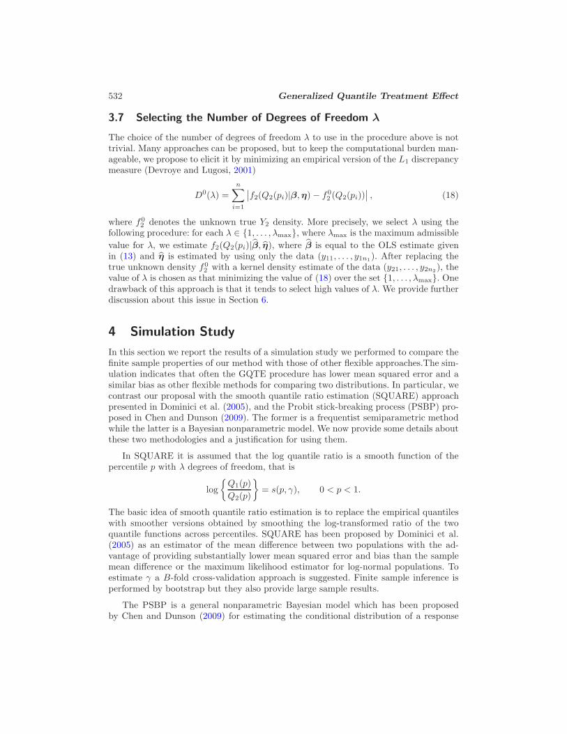
The choice of the number of degrees of freedom λ to use in the procedure above is nottrivial. Many approaches can be proposed, but to keep the computational burden man-ageable, we propose to elicit it by minimizing an empirical version of the L1 discrepancymeasure (Devroye and Lugosi, 2001)

D0(λ) =

n∑

i=1

∣∣f2(Q2(pi)|β,η)− f02 (Q2(pi))

∣∣ , (18)

where f02 denotes the unknown true Y2 density. More precisely, we select λ using the

following procedure: for each λ ∈ {1, . . . , λmax}, where λmax is the maximum admissible

value for λ, we estimate f2(Q2(pi)|β, η), where β is equal to the OLS estimate givenin (13) and η is estimated by using only the data (y11, . . . , y1n1). After replacing thetrue unknown density f0

2 with a kernel density estimate of the data (y21, . . . , y2n2), thevalue of λ is chosen as that minimizing the value of (18) over the set {1, . . . , λmax}. Onedrawback of this approach is that it tends to select high values of λ. We provide furtherdiscussion about this issue in Section 6.

4 Simulation Study

In this section we report the results of a simulation study we performed to compare thefinite sample properties of our method with those of other flexible approaches.The sim-ulation indicates that often the GQTE procedure has lower mean squared error and asimilar bias as other flexible methods for comparing two distributions. In particular, wecontrast our proposal with the smooth quantile ratio estimation (SQUARE) approachpresented in Dominici et al. (2005), and the Probit stick-breaking process (PSBP) pro-posed in Chen and Dunson (2009). The former is a frequentist semiparametric methodwhile the latter is a Bayesian nonparametric model. We now provide some details aboutthese two methodologies and a justification for using them.

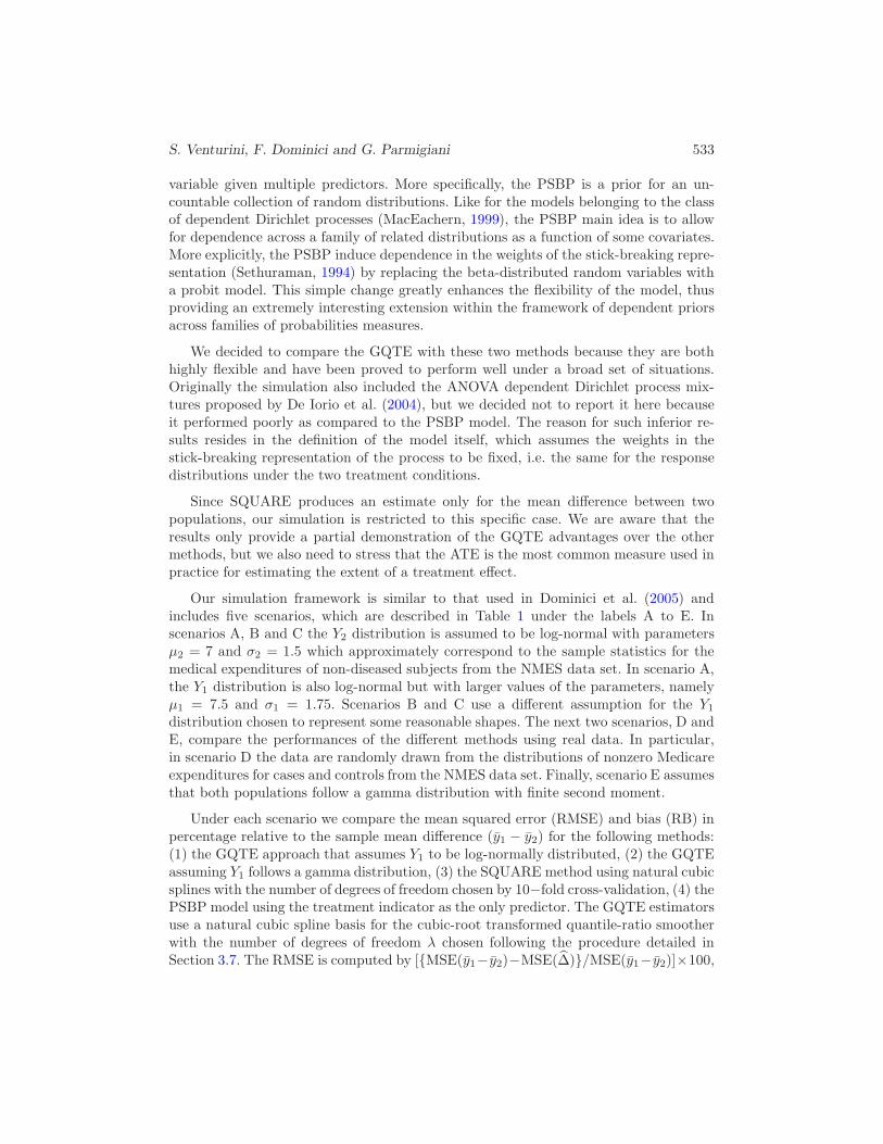
In SQUARE it is assumed that the log quantile ratio is a smooth function of thepercentile p with λ degrees of freedom, that is

log

{Q1(p)

Q2(p)

}= s(p, γ), 0 < p < 1.

The basic idea of smooth quantile ratio estimation is to replace the empirical quantileswith smoother versions obtained by smoothing the log-transformed ratio of the twoquantile functions across percentiles. SQUARE has been proposed by Dominici et al.(2005) as an estimator of the mean difference between two populations with the ad-vantage of providing substantially lower mean squared error and bias than the samplemean difference or the maximum likelihood estimator for log-normal populations. Toestimate γ a B-fold cross-validation approach is suggested. Finite sample inference isperformed by bootstrap but they also provide large sample results.

The PSBP is a general nonparametric Bayesian model which has been proposedby Chen and Dunson (2009) for estimating the conditional distribution of a response


variable given multiple predictors. More specifically, the PSBP is a prior for an un-countable collection of random distributions. Like for the models belonging to the classof dependent Dirichlet processes (MacEachern, 1999), the PSBP main idea is to allowfor dependence across a family of related distributions as a function of some covariates.More explicitly, the PSBP induce dependence in the weights of the stick-breaking repre-sentation (Sethuraman, 1994) by replacing the beta-distributed random variables witha probit model. This simple change greatly enhances the flexibility of the model, thusproviding an extremely interesting extension within the framework of dependent priorsacross families of probabilities measures.

We decided to compare the GQTE with these two methods because they are bothhighly flexible and have been proved to perform well under a broad set of situations.Originally the simulation also included the ANOVA dependent Dirichlet process mix-tures proposed by De Iorio et al. (2004), but we decided not to report it here becauseit performed poorly as compared to the PSBP model. The reason for such inferior re-sults resides in the definition of the model itself, which assumes the weights in thestick-breaking representation of the process to be fixed, i.e. the same for the responsedistributions under the two treatment conditions.

Since SQUARE produces an estimate only for the mean difference between twopopulations, our simulation is restricted to this specific case. We are aware that theresults only provide a partial demonstration of the GQTE advantages over the othermethods, but we also need to stress that the ATE is the most common measure used inpractice for estimating the extent of a treatment effect.

Our simulation framework is similar to that used in Dominici et al. (2005) andincludes five scenarios, which are described in Table 1 under the labels A to E. Inscenarios A, B and C the Y2 distribution is assumed to be log-normal with parametersµ2 = 7 and σ2 = 1.5 which approximately correspond to the sample statistics for themedical expenditures of non-diseased subjects from the NMES data set. In scenario A,the Y1 distribution is also log-normal but with larger values of the parameters, namelyµ1 = 7.5 and σ1 = 1.75. Scenarios B and C use a different assumption for the Y1

distribution chosen to represent some reasonable shapes. The next two scenarios, D andE, compare the performances of the different methods using real data. In particular,in scenario D the data are randomly drawn from the distributions of nonzero Medicareexpenditures for cases and controls from the NMES data set. Finally, scenario E assumesthat both populations follow a gamma distribution with finite second moment.

Under each scenario we compare the mean squared error (RMSE) and bias (RB) inpercentage relative to the sample mean difference (y1 − y2) for the following methods:(1) the GQTE approach that assumes Y1 to be log-normally distributed, (2) the GQTEassuming Y1 follows a gamma distribution, (3) the SQUARE method using natural cubicsplines with the number of degrees of freedom chosen by 10−fold cross-validation, (4) thePSBP model using the treatment indicator as the only predictor. The GQTE estimatorsuse a natural cubic spline basis for the cubic-root transformed quantile-ratio smootherwith the number of degrees of freedom λ chosen following the procedure detailed inSection 3.7. The RMSE is computed by [{MSE(y1−y2)−MSE(∆)}/MSE(y1−y2)]×100,


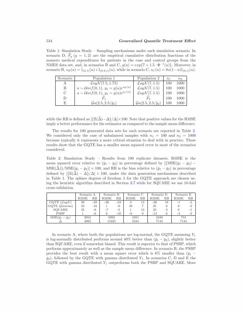
Table 1: Simulation Study – Sampling mechanisms under each simulation scenario. Inscenario D, Fg (g = 1, 2) are the empirical cumulative distribution functions of thenonzero medical expenditures for patients in the case and control groups from theNMES data set, and, in scenarios B and C, g(u) = exp{7 + 1.5 · Φ−1(u)}. Moreover, inscenario B, sB(u) = I(0,1)(u)+I(0.9,1)(u), while in scenario C, sC(u) = 8u(1−u)I(0,1)(u).

Scenario Population 1 Population 2 n1 n2

A LogN (7.5, 1.75) LogN (7, 1.5) 100 1000

B u ∼ Unif(0, 1), y1 = g(u)esB(u) LogN (7, 1.5) 100 1000C u ∼ Unif(0, 1), y1 = g(u)esC(u) LogN (7, 1.5) 100 1000

D F1 F2 100 1000E Ga(2.5, 2.5/y1) Ga(2.5, 2.5/y2) 100 1000

while the RB is defined as [{E(∆)−∆}/∆]×100. Note that positive values for the RMSEimply a better performance for the estimator as compared to the sample mean difference.

The results for 100 generated data sets for each scenario are reported in Table 2.We considered only the case of unbalanced samples with n1 = 100 and n2 = 1000because typically it represents a more critical situation to deal with in practice. Theseresults show that the GQTE has a smaller mean squared error in most of the scenariosconsidered.

Table 2: Simulation Study – Results from 100 replicate datasets. RMSE is themean squared error relative to (y1 − y2) in percentage defined by [{MSE(y1 − y2) −MSE(∆)}/MSE(y1 − y2)]× 100, and RB is the bias relative to (y1 − y2) in percentage

defined by [{E(∆) − ∆}/∆] × 100, under the data generation mechanisms describedin Table 1. The splines degrees of freedom λ for the GQTE approach are chosen us-ing the heuristic algorithm described in Section 3.7 while for SQUARE we use 10-foldcross-validation.

Scenario A Scenario B Scenario C Scenario D Scenario ERMSE RB RMSE RB RMSE RB RMSE RB RMSE RB

GQTE (LogN ) 39 -29 -26 -23 3 13 -26 18 -1 -2GQTE (Gamma) 33 -16 1 -9 48 7 25 0 0 -2

SQUARE 35 -6 -7 -5 1 13 25 3 0 -1PSBP 1 -6 6 -10 -8 9 -13 6 -3 -3

MSE(y1 − y2) 2952 5992 1051 2100 753∆ 4982 15225 5244 7144 7144

In scenario A, where both the populations are log-normal, the GQTE assuming Y1

is log-normally distributed performs around 40% better than (y1 − y2), slightly betterthan SQUARE, even if somewhat biased. This result is superior to that of PSBP, whichperforms approximately as well as the sample mean difference. In scenario B, the PSBPprovides the best result with a mean square error which is 6% smaller than (y1 −y2), followed by the GQTE with gamma distributed Y1. In scenarios C, D and E theGQTE with gamma distributed Y1 outperforms both the PSBP and SQUARE. More


specifically, in scenario C the GQTE provides a mean square error that is approximately50% smaller than (y1 − y2). This is also the least biased result. In scenarios D and E,the GQTE approach provides comparable results as those provided by SQUARE.

5 Application: Medical Costs for Smoking Attributable

Diseases

As an illustration, we apply the GQTE approach to the NMES data, where the distribu-tions of Y1 (the cases) and Y2 (the controls) are highly right-skewed. For this reason, wedecide to use h(x) = log(x). We show that having a smoking attributable disease inducesboth a location and scale shift in the medical expenditure distribution as compared tothat for non-affected subjects, but with a thinning of the corresponding distribution’stails.

5.1 Data Description

The data used in the following analysis is taken from the National Medical Expendi-ture Survey (NMES) and have been previously studied by other authors (for exampleDominici et al., 2005). It provides data on annual medical expenditures, disease status,age, race, socio-economic factors, and critical information on health risk behaviors suchas smoking, for a representative sample of U.S. non-institutionalized adults (NationalCenter For Health Services Research, 1987). NMES data derive from the 1987 wave. Inthe data set used here a total of 9,416 individuals are available. Table 3 briefly sum-marizes the data set (numbers in parentheses represent the percentage of subjects withnon-zero expenditures).

Table 3: Disease cases and controls for smokers (current or former) and for non-smokers.Numbers within parentheses represent the percentage of people in that cell with non-zero expenditures.

smokers non smokers Totalcases 165 (62%) 23 (70%) 188 (63%)controls 4,682 (21%) 4,546 (28%) 9,228 (25%)Total 4,847 (22%) 4,569 (28%) 9,416 (25%)

We consider as cases (Y1) those individuals who are affected by smoking diseases,namely lung cancer and chronic obstructive pulmonary disease, while the controls (Y2)are persons without a major smoking attributable disease.

In the following analyses we consider only the non-zero costs paid for each hospital-ization by diseased and non-diseased subjects.

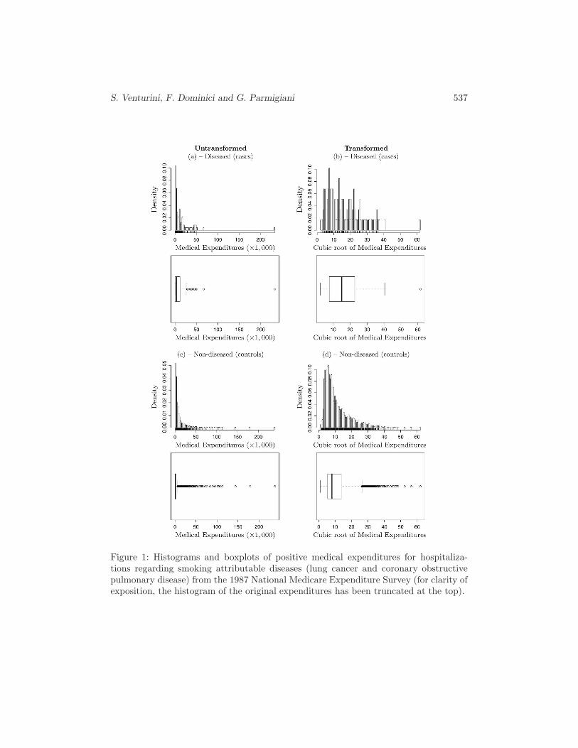
Figures 1(a) and (c) show the histograms and boxplots for the medical costs ofthe cases and controls. Both the distributions are highly right-skewed, with the casessample which is much smaller than the controls one (118 vs. 2, 262). Table 4 contains


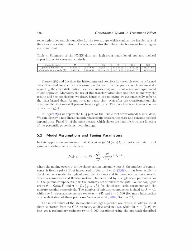
some high-order sample quantiles for the two groups which confirm the heavier tails ofthe cases costs distribution. However, note also that the controls sample has a highermaximum cost.

Table 4: Summary of the NMES data set: high-order quantiles of non-zero medicalexpenditures for cases and controls.

Quantile order 75 90 95 99 99.9 100Quantile for cases ($) 11,525.17 29,439.96 49,595.77 63,886.05 213,567.69 233,047.63

Quantile for controls ($) 2,600.00 9,799.664 30,625.206 49,771.60 135,896.07 238,185.94

Figures 1(b) and (d) show the histograms and boxplots for the cubic root transformeddata. The need for such a transformation derives from the particular choice we makeregarding the cases distribution (see next subsection) and is not a general requirementof our approach. Moreover, the use of this transformation does not alter in any way theresults and the conclusions we draw, hence in the following we systematically refer tothe transformed data. At any rate, note also that, even after the transformation, theoutcome distributions still present heavy right tails. This conclusion motivates the useof h(x) = log(x).

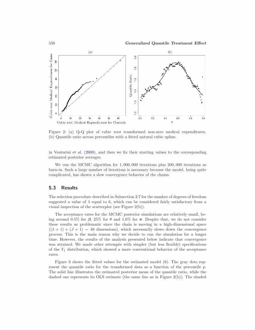
In Figure 2(a) we report the Q-Q plot for the (cubic root transformed) NMES data.We can identify a non-linear smooth relationship between the cases and controls medicalexpenditures. Panel (b) of the same picture, which shows the quantile ratio as a functionof the percentile p, confirms these findings.

5.2 Model Assumptions and Tuning Parameters

In this application we assume that Y1|π, θ ∼ GSM (π, θ|J), a particular mixture ofgamma distributions with density

f(y|π1, . . . , πJ , θ) =

J∑

j=1

πjθj

Γ(j)yj−1e−θy ,

where the mixing occurs over the shape parameters and where J , the number of compo-nents, is fixed a priori. First introduced in Venturini et al. (2008), it has been explicitlydeveloped as a model for right-skewed distributions and its parameterization allows tocreate a convenient and flexible method characterized by a single scale parameter forall the gamma components, plus the ordinary set of mixture weights. We use conjugatepriors θ ∼ Ga(α, δ) and π ∼ DJ

(1J , . . . ,

1J

)for the shared scale parameter and the

mixture weights respectively. The number of mixture components is fixed at J = 40,while the θ hyperparameters are set to α = 845 and δ = 1, 300 (for more informationon the elicitation of these priors see Venturini et al., 2008, Section 2.3).

The initial values of the Metropolis-Hastings algorithm are chosen as follows: the β

chain is started from its OLS estimate, as discussed in (13), while for η = (θ,π) wefirst get a preliminary estimate (with 5, 000 iterations) using the approach described


Figure 1: Histograms and boxplots of positive medical expenditures for hospitaliza-tions regarding smoking attributable diseases (lung cancer and coronary obstructivepulmonary disease) from the 1987 National Medicare Expenditure Survey (for clarity ofexposition, the histogram of the original expenditures has been truncated at the top).


Figure 2: (a) Q-Q plot of cubic root transformed non-zero medical expenditures.(b) Quantile ratio across percentiles with a fitted natural cubic spline.

in Venturini et al. (2008), and then we fix their starting values to the correspondingestimated posterior averages.

We run the MCMC algorithm for 1, 000, 000 iterations plus 200, 000 iterations asburn-in. Such a large number of iterations is necessary because the model, being quitecomplicated, has shown a slow convergence behavior of the chains.

5.3 Results

The selection procedure described in Subsection 3.7 for the number of degrees of freedomsuggested a value of λ equal to 6, which can be considered fairly satisfactory from avisual inspection of the scatterplot (see Figure 2(b)).

The acceptance rates for the MCMC posterior simulations are relatively small, be-ing around 0.5% for β, 25% for θ and 1.6% for π. Despite that, we do not considerthese results as problematic since the chain is moving in a high-dimensional space((λ + 1) + (J + 1) = 48 dimensions), which necessarily slows down the convergenceprocess. This is the main reason why we decide to run the simulation for a longertime. However, the results of the analysis presented below indicate that convergencewas attained. We made other attempts with simpler (but less flexible) specificationsof the Y1 distribution, which showed a more conventional behavior of the acceptancerates.

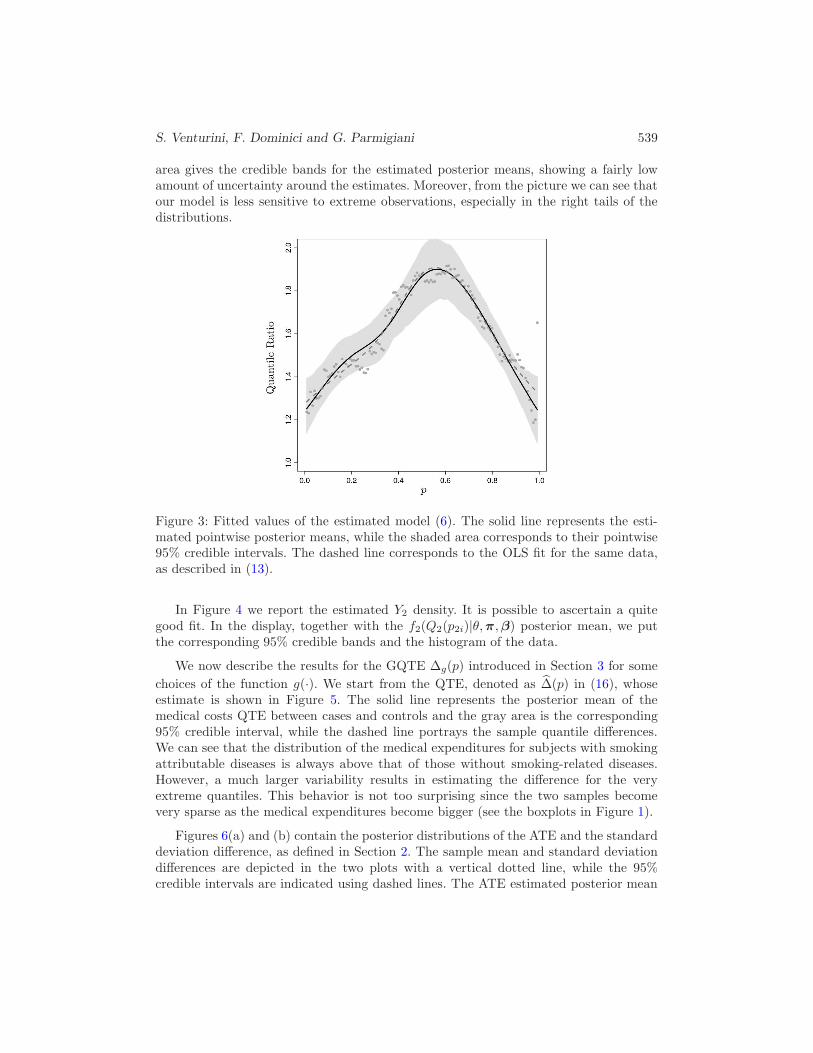
Figure 3 shows the fitted values for the estimated model (6). The gray dots rep-resent the quantile ratio for the transformed data as a function of the percentile p.The solid line illustrates the estimated posterior mean of the quantile ratio, while thedashed one represents its OLS estimate (the same line as in Figure 2(b)). The shaded


area gives the credible bands for the estimated posterior means, showing a fairly lowamount of uncertainty around the estimates. Moreover, from the picture we can see thatour model is less sensitive to extreme observations, especially in the right tails of thedistributions.

Figure 3: Fitted values of the estimated model (6). The solid line represents the esti-mated pointwise posterior means, while the shaded area corresponds to their pointwise95% credible intervals. The dashed line corresponds to the OLS fit for the same data,as described in (13).

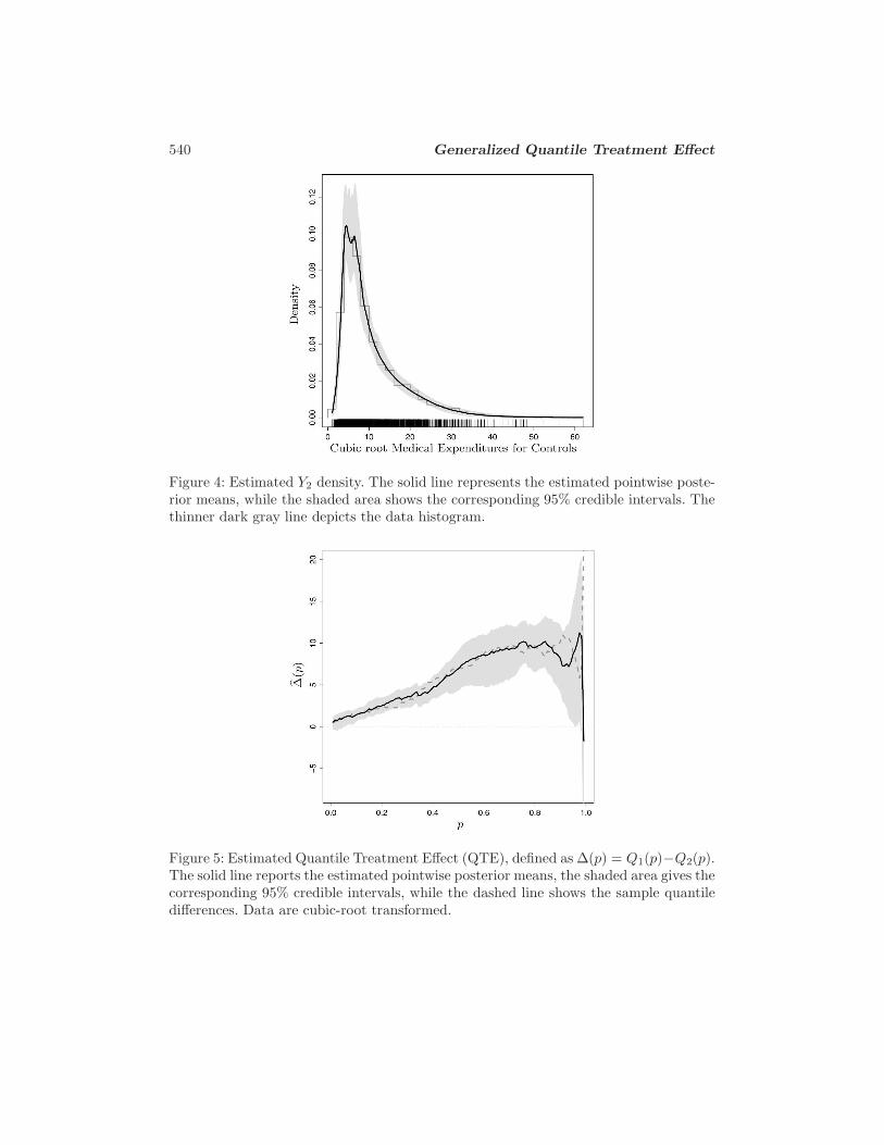
In Figure 4 we report the estimated Y2 density. It is possible to ascertain a quitegood fit. In the display, together with the f2(Q2(p2i)|θ,π,β) posterior mean, we putthe corresponding 95% credible bands and the histogram of the data.

We now describe the results for the GQTE ∆g(p) introduced in Section 3 for some

choices of the function g(·). We start from the QTE, denoted as ∆(p) in (16), whoseestimate is shown in Figure 5. The solid line represents the posterior mean of themedical costs QTE between cases and controls and the gray area is the corresponding95% credible interval, while the dashed line portrays the sample quantile differences.We can see that the distribution of the medical expenditures for subjects with smokingattributable diseases is always above that of those without smoking-related diseases.However, a much larger variability results in estimating the difference for the veryextreme quantiles. This behavior is not too surprising since the two samples becomevery sparse as the medical expenditures become bigger (see the boxplots in Figure 1).

Figures 6(a) and (b) contain the posterior distributions of the ATE and the standarddeviation difference, as defined in Section 2. The sample mean and standard deviationdifferences are depicted in the two plots with a vertical dotted line, while the 95%credible intervals are indicated using dashed lines. The ATE estimated posterior mean


Figure 4: Estimated Y2 density. The solid line represents the estimated pointwise poste-rior means, while the shaded area shows the corresponding 95% credible intervals. Thethinner dark gray line depicts the data histogram.

Figure 5: Estimated Quantile Treatment Effect (QTE), defined as ∆(p) = Q1(p)−Q2(p).The solid line reports the estimated pointwise posterior means, the shaded area gives thecorresponding 95% credible intervals, while the dashed line shows the sample quantiledifferences. Data are cubic-root transformed.


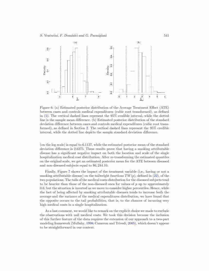
Figure 6: (a) Estimated posterior distribution of the Average Treatment Effect (ATE)between cases and controls medical expenditures (cubic root transformed), as definedin (5). The vertical dashed lines represent the 95% credible interval, while the dottedline is the sample mean difference. (b) Estimated posterior distribution of the standarddeviation difference between cases and controls medical expenditures (cubic root trans-formed), as defined in Section 2. The vertical dashed lines represent the 95% credibleinterval, while the dotted line depicts the sample standard deviation difference.

(on the log scale) is equal to 6.1127, while the estimated posterior mean of the standarddeviation difference is 2.6275. These results prove that having a smoking attributabledisease has a significant negative impact on both the location and scale of the singlehospitalization medical cost distribution. After re-transforming the estimated quantileson the original scale, we get an estimated posterior mean for the ATE between diseasedand non-diseased subjects equal to $6, 244.10.

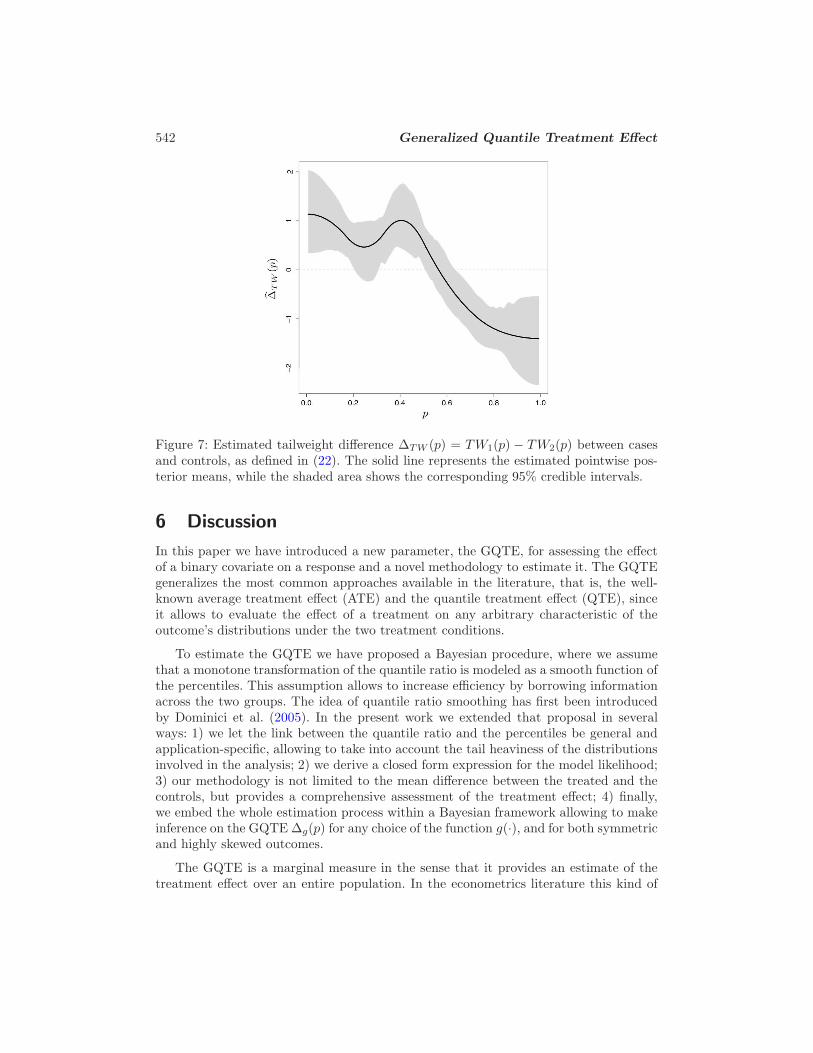
Finally, Figure 7 shows the impact of the treatment variable (i.e., having or not asmoking attributable disease) on the tailweight functions TW (p), defined in (22), of thetwo populations. The tails of the medical costs distribution for the diseased subjects tendto be heavier than those of the non-diseased ones for values of p up to approximately0.6, but the situation is inverted as we move to consider higher percentiles. Hence, whilethe fact of being affected by smoking attributable diseases tends to increase both theaverage and the variance of the medical expenditures distribution, we have found thatthe opposite occurs to the tail probabilities, that is, to the chances of incurring veryhigh medical costs in a single hospitalization.

As a last comment, we would like to remark on the explicit choice we made to excludethe observations with null medical costs. We took this decision because the inclusionof this further feature of the data requires the extension of our approach to a two-partmodeling framework (Mullahy, 1998; Cameron and Trivedi, 2005), which doesn’t appearto be straightforward in our context.


Figure 7: Estimated tailweight difference ∆TW (p) = TW1(p) − TW2(p) between casesand controls, as defined in (22). The solid line represents the estimated pointwise pos-terior means, while the shaded area shows the corresponding 95% credible intervals.

6 Discussion

In this paper we have introduced a new parameter, the GQTE, for assessing the effectof a binary covariate on a response and a novel methodology to estimate it. The GQTEgeneralizes the most common approaches available in the literature, that is, the well-known average treatment effect (ATE) and the quantile treatment effect (QTE), sinceit allows to evaluate the effect of a treatment on any arbitrary characteristic of theoutcome’s distributions under the two treatment conditions.

To estimate the GQTE we have proposed a Bayesian procedure, where we assumethat a monotone transformation of the quantile ratio is modeled as a smooth function ofthe percentiles. This assumption allows to increase efficiency by borrowing informationacross the two groups. The idea of quantile ratio smoothing has first been introducedby Dominici et al. (2005). In the present work we extended that proposal in severalways: 1) we let the link between the quantile ratio and the percentiles be general andapplication-specific, allowing to take into account the tail heaviness of the distributionsinvolved in the analysis; 2) we derive a closed form expression for the model likelihood;3) our methodology is not limited to the mean difference between the treated and thecontrols, but provides a comprehensive assessment of the treatment effect; 4) finally,we embed the whole estimation process within a Bayesian framework allowing to makeinference on the GQTE ∆g(p) for any choice of the function g(·), and for both symmetricand highly skewed outcomes.

The GQTE is a marginal measure in the sense that it provides an estimate of thetreatment effect over an entire population. In the econometrics literature this kind of


approach is usually termed the unconditional QTE (Firpo, 2007; Frolich and Melly,2008) in contrast with the conditional QTE, where the treatment effect is determinedseparately for different combinations of a set of covariates (Koenker and Bassett, 1978;Koenker, 2005; Angrist and Pischke, 2009). The inclusion of covariates can improve theefficiency of an estimator even when the primary goal of the analysis is a marginal effect.Accordingly, methods have been proposed to extract marginal quantiles from estimatesof conditional quantiles (Machado and Mata, 2005; Frolich and Melly, 2008). A challengein extending our approach along these lines is the lack of an “iterated expectation”result1 for the quantiles (see for example Angrist and Pischke, 2009, Chapter 7).

To further clarify our goals, we want to stress that in this paper no particularemphasis has been placed on the causality issues that naturally comes into play whenthe objective is the estimation of a treatment effect (see for example Rosenbaum, 2002,2010; Rubin, 2006; Angrist and Pischke, 2009). More precisely, our intent here is solelyto provide a general measure of the effect of a binary treatment on a response variable,together with a flexible approach to estimate it.

We compared the performance of our estimation approach with other highly flexiblemethods in a simulation study for the mean difference between two populations. Ourstudy revealed that the GQTE performs generally better than the other competingestimators at least in estimating the mean difference.

We have applied our methodology to the NMES data set to assess the effect of beingaffected by smoking attributable diseases on the single hospitalization medical costsdistribution. We have found that having these diseases increases the average medicalbill amount as well as its variability in the population, while it reduces the probabilityof incurring higher bills.

Our approach can be extended in various directions. The most promising researchquestion we can see involves taking into account individual level characteristics in mea-suring the effect of a treatment. In our context, this would involve the estimation of aconditional version of ∆g(p), something like ∆g(p|x) = g (Q1(p|x)) − g (Q2(p|x)). Theclear advantage of including covariates would be an increase in the efficiency of theestimates (Frolich and Melly, 2008). To control for systematic differences in covariatesbetween two populations, a common strategy is to group units into subclasses based oncovariate values, for example using propensity score matching, and then to apply ourmethod within strata of propensity scores (Rosenbaum, 2002, 2010), as implementedfor example in Dominici and Zeger (2005).

Currently we are considering only a binary treatment effect, so another importantline of research is the extension of the methods to categorical ordinal and to continuoustreatments.

A further direction for future research concerns the choice of the number of degreesof freedom λ. In this paper we adopted the simple approach of choosing λ by minimizingan empirical version of the L1 distance between the Y2 density estimate and its kerneldensity estimate (see Subsection 3.7). More structured solutions can obviously be con-

1While for a standard linear model, in fact, the assumption E(Yi|Xi) = X′iβ does imply E(Yi) =

E(Xi)′β, the same conclusion doesn’t hold for the conditional quantiles.


sidered. A natural extension would allow λ to be a random quantity to be estimatedtogether with all the other parameters using a trans-dimensional MCMC approach, likefor example the reversible jump algorithm (Green, 1995). While this solution wouldallow to take into account also the uncertainty connected to the a priori ignoranceabout the λ value, the consequence would be a dramatic increase in the computationalworkload of the estimation algorithm.

Acknowledgements

The research of Dominici was supported by Award Number R01ES012054 (StatisticalMethods for Population Health Research on Chemical Mixtures) from NIH/NIEHS,Award Numbers R83622 (Statistical Models for Estimating the Health Impact of AirQuality Regulations) and RD83241701 (Estimation of the Risks to Human Health of PMand PM Components) from EPA, Award Number 4909-RFA11-1/12-3 (Causal InferenceMethods for Estimating Long Term Health Effects of Air Quality Regulations) from HEIand Award Number K18 HS021991 (A Translational Framework for MethodologicalRigor to Improve Patient Centered Outcomes in End of Life Cancer Research) fromAHRQ. The content is solely the responsibility of the authors and does not necessarilyrepresent the official views of the above Institutions.

Appendix 1: Additional GQTE Examples

Together with the cases presented in Section 2, many other less conventional measuresof the difference between two distributions can be obtained by properly choosing the g(·)function in the GQTE definition. For example, by choosing g(x) =

∫xr dp we obtain

the difference between the population r-th moments

∆µr =

∫ 1

0

Q1(p)r dp−

∫ 1

0

Q2(p)r dp. (19)

Using the fact that for a random variable Y with expected value µ, variance σ2 andquantile function Q(p) it holds that (see Gilchrist, 2000 or Shorack, 2000)

σ2 =

∫ 1

0

[Q(p)− µ]2dp =

∫ 1

0

Q(p)2 dp− µ2,

by suitably choosing the g(·) function, we recover the difference between the two pop-ulation variances as

∆σ2 =

[∫ 1

0

Q1(p)2 dp−

(∫ 1

0

Q1(p) dp

)2]−[∫ 1

0

Q2(p)2 dp−

(∫ 1

0

Q2(p) dp

)2]

=

[∫ 1

0

Q1(p)2 dp−

∫ 1

0

Q2(p)2 dp

]−[(∫ 1

0

Q1(p) dp

)2

−(∫ 1

0

Q2(p) dp

)2]

= ∆µ2 −(µ21 − µ2

2

), (20)


However, the cases encompassed by the GQTE include many other quantile-basedindexes that are less frequently used in the literature, like the inter-p-range ipr(p) =Q(1 − p) − Q(p), or the skewness-ratio sr(p) = [Q(1 − p) − Q(0.5)]/[Q(0.5) − Q(p)],0 < p < 1, which provide robust measures of the scale and shape of a distribution (for alist of these indexes see Gilchrist, 2000; Shorack, 2000; Parzen, 2004; Wang and Serfling,2005; Brys et al., 2006). A quantity of particular interest to economists is the differencebetween inter-decile ratios, defined as

Q1(0.9)

Q1(0.1)− Q2(0.9)

Q2(0.1),

which is commonly used to measure the inequality in a population (see Frolich andMelly, 2008). The previous quantity can be easily generalized as follows

∆IR(p) =Q1(1− p)

Q1(p)− Q2(1− p)

Q2(p), (21)

for any 0 < p < 0.5. Notice that all these indexes are obtainable from the generaldefinition (3) by properly choosing the function g(·).

As a last example, we consider a further GQTE special case that is based on the socalled tailweight function defined as

TW (p) =q(p)

Q(p)≡ d

dplogQ(p) , 0 < p < 1 ,

which is used to quantify the probability allocated in the tails of a distribution. One cancompute the difference between the tailweight functions for two populations by choosingthe logarithmic derivative of the quantile function as the g(·) functional in (3), that is

∆TW (p) = TW1(p)− TW2(p)

=d

dplogQ1(p)−

d

dplogQ2(p)

=d

dp

[log

(Q1(p)

Q2(p)

)]. (22)

If ∆TW (p) ≥ 0, we can conclude that the treatment is causing a thickening of the Y1

distribution tails as compared to those of Y2 if ∆TW (p) ≥ 0. Finally, note that, thanksto the equivariance property of the quantiles, (22) can be written also as

∆TW (p) =d

dplogQ1(p)−

d

dplogQ2(p)

=d

dpQ1,log(p)−

d

dpQ2,log(p)

=d

dp[Q1,log(p)−Q2,log(p)]

=d

dp∆log(p) , (23)

where Qℓ,log, ℓ = 1, 2, indicates the quantile of the log-transformed data and ∆log(p)denotes the parameter (4) calculated on the quantiles of the log-transformed data.


Appendix 2: Proof of Theorem 1 and Corollaries

Proof of Theorem 1. Differentiate (7) with respect to p to get

q1(p) = q2(p)h−1 [X(p, λ)β] +X ′(p, λ)βQ2(p)

{d

d (X(p, λ)β)h−1 [X(p, λ)β]

}, (24)

where qℓ(p) = dQℓ(p)/dp denotes the so called quantile density function for the pop-ulation ℓ = {1, 2}, while X ′(p, λ) corresponds to the derivative of X(p, λ), 0 < p < 1(properly resized because a constant is normally included in the design matrix X(p, λ)).

Apply now to both q1(p) and q2(p) the following relationship between the quantiledensity and density quantile functions (see for example Gilchrist, 2000; Parzen, 1979,2004)

f(Q(p)) q(p) = 1 , (25)

to get the expression

1

f1(Q1(p)|η)=

1

f2(Q2(p)|β,η)h−1 [X(p, λ)β]

+X ′(p, λ)βQ2(p)

{d

d (X(p, λ)β)h−1 [X(p, λ)β]

}, (26)

and hence

f2(Q2(p)|β,η) = f1(Q1(p)|η)h−1[X(p,λ)β]

1−f1(Q1(p)|η)X′(p,λ)βQ2(p){ dd(X(p,λ) β)

h−1[X(p,λ)β]} . (27)

Finally, substituting (7) in place of Q1(p) proves the main statement.

Moreover, f2(Q2(p)|β,η) is a proper density function because:

• f2(Q2(p)|β,η) ≥ 0, for any 0 < p < 1; since f1 (Q1(p)|η) ≥ 0 and h−1 [X(p, λ)β] >0 because, as assumed in (6), it is the ratio of two positive quantile functions, thisfact can be proved by showing that the denominator of (27) is nonnegative whichis ensured by the constraint (10).

•∫ 1

0f2(Q2(p)|β,η)q2(p)dp = 1, which is true because f2(Q2(p)|β,η)q2(p) = 1 by

construction.

A couple of immediate consequences of Theorem 1 regard two cases that occurfrequently in practice. We provide the details about these situations in the next twocorollaries.

Corollary 1. Let the same assumptions of Theorem 1 hold. Suppose additionally thath(x) = x. If for every 0 < p < 1 the vector β satisfies the constraint

X ′(p, λ)β

X(p, λ)β≤ 1

f1 (Q1(p))Q1(p), (28)


then the density quantile function f2(Q2(p)|β,η) for Y2 is

f2(Q2(p)|β,η) =f1 (Q2(p)X(p, λ)β|η)X(p, λ)β

1− f1 (Q2(p)X(p, λ)β|η)X ′(p, λ)βQ2(p). (29)

Corollary 2. Let the same assumptions of Theorem 1 hold. Suppose additionally thath(x) = log(x). If for every 0 < p < 1 the vector β satisfies the constraint

X ′(p, λ)β ≤ 1

f1 (Q1(p))Q1(p), (30)

then the density quantile function f2(Q2(p)|β,η) for Y2 is given by

f2(Q2(p)|β,η) =f1(Q2(p) e

X(p,λ)β|η)

e−X(p,λ)β − f1(Q2(p) eX(p,λ)β|η

)X ′(p, λ)βQ2(p)

. (31)

Note that in these two situations, the general constraint (10) reduces to a linearconstraint on β.

Appendix 3: Proofs of the Special Cases

Case 1: Y1 is Uniform and X(p, λ = 0) = 1. Here Y1|θ1 ∼ U [ 0, θ1] and h(x) = x. Inthis case Q1(p)/Q2(p) = β0. Hence the density, distribution and quantile functions ofY1 are respectively

f1(y1|θ1) =1

θ1I[0, θ1]{y1}

F1(y1|θ1) =y1θ1

Q1(p|θ1) = θ1p , 0 < p < 1 .

From (29) it follows that

f2(Q2(p)|θ1, β0) =1

θ1I[0, θ1]{Q2(p)β0} β0

=β0

θ1I[0, θ1/β0]{Q2(p)} ,

which is the density quantile function of a U [0, θ2] random variable with θ2 = θ1/β0.

Case 2: Y1 is Log-normal and X(p, λ = 1) = [1,Φ−1(p)]. Assume Y1|µ1, σ21 ∼ Ln(µ1, σ

21)

and h(x) = log(x). In this case log{Q1(p)/Q2(p)} = β0 + β1 Φ−1(p), where Φ−1(p) is

the quantile function of a standard normal random variable. The density, distributionand quantile functions of Y1 are given by

f1(y1|µ1, σ21) =

1

y1√2πσ1

exp

{− (log y1 − µ1)

2

2σ21

}


F1(y1|µ1, σ21) = Φ

(log y1 − µ1

σ1

)

Q1(p|µ1, σ21) = exp

{µ1 + σ1Φ

−1(p)}, 0 < p < 1 .

Then by (31) it follows

f2(Q2(p)|µ1, σ21 , β0, β1) =

1√2πσ1

exp

− (µ1+σ1Φ−1(p)−µ1)2

2σ21

exp{µ1+σ1Φ−1(p)}

exp {−β0 − β1Φ−1(p)}

1− 1√2πσ1

exp

− (µ1+σ1Φ−1(p)−µ1)2

2σ21

exp{µ1+σ1Φ−1(p)}

×β11

1√2π

exp

− [Φ−1(p)]22

exp {µ1 + σ1Φ−1(p)}

=1√

2π(σ1 − β1)

exp

{

− [Φ−1(p)]2

2

}

exp { (µ1 − β0) + (σ1 − β1)Φ−1(p)}

=1√

2π(σ1 − β1)

exp

{

− [(µ1−β0)+(σ1−β1)Φ−1(p)−(µ1−β0)]

2

2(σ1−β1)2

}

exp { (µ1 − β0) + (σ1 − β1)Φ−1(p)}

=1

Q2(p)√2π(σ1 − β1)

exp

{

− [logQ2(p)− (µ1 − β0)]2

2(σ1 − β1)2

}

,

which is the density quantile function of a Ln(µ2, σ22) random variable with µ2 = (µ1 −

β0) and σ2 = (σ1 − β1).

Case 3: Y1 is Pareto and X(p, λ = 1) = [1, log(1 − p)]. Now Y1|a1, b1 ∼ Pa(a1, b1)and h(x) = log(x). In this case log{Q1(p)/Q2(p)} = β0 + β1 log(1 − p). The density,distribution and quantile functions of Y1 are given by

f1(y1|a1, b1) = a1ba11 y

−(a1+1)1

F1(y1|a1, b1) = 1− ba11 y−a1

1

Q1(p|a1, b1) = b1(1 − p)−1a1 , 0 < p < 1 .

Then (31) implies

f2(Q2(p)|a1, b1, β0, β1) =a1b

a11

[

b1(1−p)− 1

a1

]−(a1+1)

exp{−β0−β1 log(1−p)}

1+a1ba11

[

b1(1−p)− 1

a1

]−(a1+1)β11−p

b1(1−p)− 1

a1

=a1

a1β1 + 1

(

b1e−β0

)−1

(1− p)a1β1+1

a1+1

=a1

a1β1 + 1

(

b1e−β0

)

a1a1β1+1

Q2(p)−(

a1a1β1+1

+1)

,


which is the density quantile function of a Pa(a2, b2) random variable with a2 = a1

a1β1+1

and b2 = b1e−β0 .

Appendix 4: Details About the Estimation of Other Cases

One can estimate the impact of a binary treatment on the r-th moments, denoted as∆µr in (19), by computing

∆(m)µr =

1

n2

n2∑

i=1

{y2(i)h

−1

[X (p2i, λ) β

(m)]}r

− 1

n1

n1∑

i=1

[y1(i)

{h−1

[X (p1i, λ) β

(m)]}−1

]r. (32)

The last expression allows to estimate the treatment effect on the population variances,defined in (20), which is given by

∆(m)σ2 = ∆

(m)µ2 −

(1

n2

n2∑

i=1

y2(i)h−1

[X (p2i, λ) β

(m)])2

−(

1

n1

n1∑

i=1

y1(i)

{h−1

[X (p1i, λ) β

(m)]}−1

)2 . (33)

As a concluding example, the effect of a binary treatment on the tailweight functionsof two distributions, introduced in (22), can be obtained by first computing the posteriordraws

∆(m)TW (p) =

d

dp

{log

(h−1

[X(p, λ)β

(m)])}

, (34)

and then by applying (15). When h(x) = log(x), (34) becomes

∆(m)TW (p) = X ′(p, λ)β

(m), (35)

and the estimate of ∆TW (p) is

∆TW (p) =1

M

M∑

m=1

X ′(p, λ)β(m)

= X ′(p, λ)

(1

M

M∑

m=1

β(m)

)

= X ′(p, λ)β, (36)

with β = 1M

∑Mm=1 β

(m), the posterior mean estimate of β.


ReferencesAbadie, A., Angrist, J. D., and Imbens, G. (2002). “Instrumental variables estimates ofthe effect of subsidized training on the quantiles of trainee earnings.” Econometrica,70: 91–117. 524

Angrist, J. D. and Pischke, J.-S. (2009). Mostly harmless econometrics . PrincetonUniversity Press, Princeton, NJ. 543

Brys, G., Hubert, M., and Struyf, A. (2006). “Robust measures of tail weight.” Com-putational Statistics & Data Analysis , 50(3): 733–759. 545

Cameron, C. A. and Trivedi, P. K. (2005). Microeconometrics . Cambridge UniversityPress, New York. 541

Carlin, B. P. and Louis, T. A. (2009). Bayesian methods for data analysis . Chapman& Hall/CRC, Boca Raton, Third edition. 530

Chen, Y. and Dunson, D. B. (2009). “Nonparametric Bayes conditional distributionmodeling with variable selection.” Journal of the American Statistical Association,104(488): 1646–1660. 532

Chernozhukov, V. and Hansen, C. (2005). “An IV model of quantile treatment effects.”Econometrica, 73: 245–261. 524

De Iorio, M., Muller, P., Ronser, G. L., and MacEachern, S. N. (2004). “An ANOVAmodel for dependent random measures.” Journal of the American Statistical Associ-ation, 99(465): 205–215. 533

Devroye, L. and Lugosi, G. (2001). Combinatorial methods in density estimation.Springer. 532

Dominici, F., Cope, L., Naiman, D. Q., and Zeger, S. L. (2005). “Smooth quantile ratioestimation (SQUARE).” Biometrika, 92: 543–557. 523, 524, 526, 532, 533, 535, 542

Dominici, F. and Zeger, S. L. (2005). “Smooth quantile ratio estimation with regression:estimating medical expenditures for smoking-attributable diseases.” Biostatistics , 6:505–519. 543

Dominici, F., Zeger, S. L., Parmigiani, G., Katz, J., and Christian, P. (2006). “Esti-mating percentile-specific treatment effects in counterfactual models: a case-study ofmicronutrient supplementation, birth weight and infant mortality.” Journal of theRoyal Statistical Society: Series C (Applied Statistics), 55: 261–280. 525

— (2007). “Does the effect of micronutrient supplementation on neonatal survival varywith respect to the percentiles of the birth weight distribution?” Bayesian Analysis ,2: 1–30. 525

Firpo, S. (2007). “Efficient semiparametric estimation of quantile treatment effects.”Econometrica, 75: 259–276. 524, 543

Frolich, M. and Melly, B. (2008). “Unconditional quantile treatment effects under en-dogeneity.” Technical Report 3288, Institute for the Study of Labor (IZA), P.O. Box7240, 53072 Bonn, Germany. 524, 525, 543, 545


Gelman, A., Carlin, J. B., Stern, H. S., Dunson, D. B., Vehtari, A., and Rubin, D. B.(2013). Bayesian data analysis . Chapman & Hall/CRC, Boca Raton, Third edition.531

Gilchrist, W. G. (2000). Statistical modelling with quantile functions . Chapman &Hall/CRC, New York. 528, 544, 545, 546

Gilks, W. R., Richardson, S., and Spiegelhalter, D. J. (eds.) (1996). Markov ChainMonte Carlo in practice. Chapman & Hall/CRC, New York. 530

Green, P. J. (1995). “Reversible jump MCMC computation and Bayesian model deter-mination.” Biometrika, 82(4): 711–732. 544

Koenker, R. (2005). Quantile regression. Cambridge University Press, New York. 543

Koenker, R. and Bassett, G. S. (1978). “Regression quantiles.” Econometrica, 46: 33–50.543

MacEachern, S. N. (1999). “Dependent Nonparametric Processes.” In ASA Proceedingsof the Section on Bayesian Statistical Science. Alexandria, VA: American StatisticalAssociation. 533

Machado, J. and Mata, J. (2005). “Counterfactual decompositions of changes in wagedistributions using quantile regression.” Journal of Applied Econometrics , 20: 445–465. 543

Mullahy, J. (1998). “Much ado about two: reconsidering retransformation and the two-part model in health econometrics.” Journal of Health Economics , 17: 247–281. 541

National Center For Health Services Research (1987). National Medical ExpenditureSurvey. National Center for Health Services Research and Health Technology Assess-ment. 535

O’Hagan, G. and Forster, J. (2004). Bayesian inference. Arnold, London, Secondedition. 530

Parzen, E. (1979). “Nonparametric statistical data modeling.” Journal of the AmericanStatistical Association, 74: 105–121. 528, 546

— (2004). “Quantile probability and statistical data modeling.” Statistical Science, 19:652–662. 545, 546

Robert, C. P. and Casella, G. (2004). Monte Carlo statistical methods . Springer, NewYork, Second edition. 530

Rosenbaum, P. (2002). Observational studies . Springer, New York. 543

— (2010). Design of observational studies . Springer, New York. 543

Rubin, D. B. (2006). Matched sampling for causal effects . Cambridge University Press,Cambridge, UK. 543

Sethuraman, J. (1994). “A constructive definition of Dirichlet priors.” Statistica Sinica,4: 639–650. 533


Shorack, G. R. (2000). Probability for statisticians . Springer, New York. 544, 545

Venturini, S., Dominici, F., and Parmigiani, G. (2008). “Gamma shape mixtures forheavy-tailed distributions.” Annals of Applied Statistics , 2: 756–776. 536, 538

Wang, J. and Serfling, R. (2005). “Nonparametric multivariate kurtosis and tailweightmeasures.” Journal of Nonparametric Statistics , 17: 441–456. 545

Wooldridge, J. M. (2010). Econometric analysis of cross section and panel data. MITPress, Second edition. 525

Documents

Generalized Quantile Treatment Effect: A Flexible … · A Flexible Bayesian Approach Using Quantile Ratio Smoothing Sergio Venturini ... S.Venturini,F.DominiciandG.Parmigiani 525