Geometric Shape Preservation in Adaptive Refinement of - KTH

Geometric Shape Preservation in Adaptive Refinement

of Finite Element Meshes

A S H R A F U L K A D I R

Master of Science Thesis Stockholm, Sweden 2010

Geometric Shape Preservation in Adaptive Refinement

of Finite Element Meshes

A S H R A F U L K A D I R

Master’s Thesis in Numerical Analysis (30 ECTS credits) at the Scientific Computing International Master Program Royal Institute of Technology year 2010 Supervisor at CSC was Johan Hoffman Examiner was Michael Hanke TRITA-CSC-E 2010:001 ISRN-KTH/CSC/E--10/001--SE ISSN-1653-5715 Royal Institute of Technology School of Computer Science and Communication KTH CSC SE-100 44 Stockholm, Sweden URL: www.csc.kth.se

AbstractThis thesis presents a vertex repositioning based boundary smoothing techniqueso that the finite element mesh, as refined, converges to the geometric shape ofthe domain. Adaptive mesh refinements based on a posteriori error estimates isalready available within FEniCS, a free software for automated solution of differ-ential equations. However, as the refinement process runs independently of theCAD (Computer-Aided Design) data, once the initial mesh is created the geomet-ric shape is fixed and remains unchanged. The proposed technique removes thislimitation enabling the mesh to be reshaped during the mesh refinement processaccording to the geometry. In the proposed technique, upon mesh refinements,the boundary vertices are repositioned to the orthogonal projection point on tothe surface geometry. Newton iteration based iterative closest point algorithmshave been used to search points projection on to the geometry represented asNURBS (Nonuniform Rational B-splines). For the new boundary vertices, oldneighbor-nodes’ projection data have been used for obtaining an initial guess forthe Newton’s iteration. Projection parameters for the boundary vertices of aninitial coarse mesh is gathered using exhaustive search for points projection onthe whole geometry. Once the mesh boundary vertices are repositioned, positionsof the internal vertices are adjusted using mesh smoothing. Experimental resultsshow that the method is sufficiently accurate and efficient for both 2D and 3Dproblems for some simple test cases. Inverted cells, which could invalidate themesh, are not developed. Cell based mesh quality analysis and time performanceanalysis have been presented. Experimentally, it has been shown that using theproposed technique it is sufficient to start with a coarse mesh all over the do-main and adaptively refine the mesh and the coarse mesh, as refined, capturesthe curved geometry more accurately. Since the proposed technique does notchange the mesh topology and the finite element solver or mesh elements arenot required to be changed, the developed tools can be plugged in to the finiteelement solver without much involvements. Although the tools are developedto become integrated parts of FEniCS, the parts representing geometric datamanipulation can be used with other applications as well. Implementations inthis thesis are limited for single NURBS patch geometry only and recommenda-tions are given for future improvements to incorporate multiple patch NURBSgeometry and trimmed NURBS.

ReferatBevarande av geometrisk form i

finita elementmetoder med adaptiv nätförfining

I den här avhandlingen presenteras en teknik för anpassning av randnoder, såatt beräkningsnätet under förfining konvergerar till den exakta geometriska do-mänen. Adaptiv nätförfining baserat på a posteriori-feluppskattning finns redani FEniCS: fri mjukvara för automatiserad lösning av differentialekvationer. Docksaknas kopplingen mellan CAD (geometri) och nätförfining så efter det ursprung-liga nätet har skapats tas inte längre någon hänsyn till geometrin. Den presente-rade tekniken tar bort denna begränsning och möjliggör en anpassning av nätettill geometrin under nätförfiningsprocessen. I den presenterade tekniken flyttasrandnoder, efter nätförfining, till den ortogonalt projicerade punkten på ytan avrandgeometrin. Iterativa Newton-algoritmer har använts för att söka efter pro-jektionspunkter på geometri representerad som NURBS (Nonuniform RationalB-splines). För att behandla de nya randnoderna har projektionsdata från grann-noder använts som en gissning till Newton-iterationen. Projektionsparametrar förrandnoderna i ett ursprungligt grovt nät insamlas med en uttömmande sökningför projektionspunkter i hela geometrin. När anpassningen av randnoderna hargjorts flyttas de interna noderna enligt en utslätningsmetod. Experiment visaratt metoden ger tillräcklig noggrannhet och effektivitet för enkla 2D och 3D-problem. Inverterade celler genereras ej. Tekniken ämnas integreras i FEniCS,men kan även användas självständigt. Implementationen som ges i avhandlingenär begränsad för en ensam NURBS-yta men rekommendationer ges för framtidautökning för multipla NURBS-ytor och trimmade ytor.

Acknowledgements

First, I would like to say thanks to my supervisor, Prof. Johan Hoffman, for givingme the opportunity to work in this interesting project and for his excellent guidancethroughout the period. I would also like to say thanks to Prof. Michael Hanke forreading the manuscript and advising valuable improvements. I would like to saythanks to Johan Jansson for the interesting discussions, sharing his knowledge onFEniCS, and finally for translating the abstract of the thesis for me. I also thankMurtazo Nazarov for sharing his ideas and knowledge on FEniCS. I would alsolike to say thanks to the other members of the CTL (Computational TechnologyLaboratory) group for the interesting discussions and support.

I thank my loving wife for her understanding, encouragements and support.Finally, I dedicate my thesis to my wonderful parents for their love, encouragementsand unconditional support throughout my life. I specially acknowledge my mother’sgreat contributions to my life who dedicated all her efforts for her two sons.

Contents

1 Introduction 11.1 Related Works . . . . . . . . . . . . . . . . . . . . . . . . . . . . . . 21.2 Motivation . . . . . . . . . . . . . . . . . . . . . . . . . . . . . . . . 41.3 Outline . . . . . . . . . . . . . . . . . . . . . . . . . . . . . . . . . . 5

2 Mesh Boundary Smoothing 72.1 Point Projection on Curves and Surfaces . . . . . . . . . . . . . . . . 7

2.1.1 Point Projection Algorithms: a Literature Review . . . . . . 82.2 Boundary Smoothing Algorithm . . . . . . . . . . . . . . . . . . . . 102.3 Neighbor Information based Searching . . . . . . . . . . . . . . . . . 10

2.3.1 Initializing a Mesh . . . . . . . . . . . . . . . . . . . . . . . . 102.3.2 Storing Information with Mesh Nodes . . . . . . . . . . . . . 112.3.3 Finding and using Neighbors’ Information . . . . . . . . . . . 132.3.4 Searching in a NURBS Array . . . . . . . . . . . . . . . . . . 142.3.5 Time Complexity . . . . . . . . . . . . . . . . . . . . . . . . . 15

3 Implementation 173.1 FEniCS . . . . . . . . . . . . . . . . . . . . . . . . . . . . . . . . . . 17

3.1.1 DOLFIN . . . . . . . . . . . . . . . . . . . . . . . . . . . . . 183.1.2 UNICORN . . . . . . . . . . . . . . . . . . . . . . . . . . . . 18

3.2 NURBS++ . . . . . . . . . . . . . . . . . . . . . . . . . . . . . . . . 183.3 Implementation of the Geometry Library . . . . . . . . . . . . . . . 193.4 Integration with FEniCS . . . . . . . . . . . . . . . . . . . . . . . . . 19

3.4.1 Implementation of the Boundary Smoothing Tool . . . . . . . 193.4.2 Running the Systems . . . . . . . . . . . . . . . . . . . . . . . 21

4 Results 234.1 Performance . . . . . . . . . . . . . . . . . . . . . . . . . . . . . . . . 254.2 Mesh Quality . . . . . . . . . . . . . . . . . . . . . . . . . . . . . . . 284.3 Boundary Smoothing with Adaptive Refinements . . . . . . . . . . . 29

5 Conclusion 335.1 Future Works . . . . . . . . . . . . . . . . . . . . . . . . . . . . . . . 34

Bibliography 35

A Introduction to Curves and Surfaces 39A.1 Explicit equations . . . . . . . . . . . . . . . . . . . . . . . . . . . . 39A.2 Implicit equations . . . . . . . . . . . . . . . . . . . . . . . . . . . . 40A.3 Parametric functions . . . . . . . . . . . . . . . . . . . . . . . . . . . 41

A.3.1 Parametric Polynomial Curves . . . . . . . . . . . . . . . . . 42A.3.2 Parametric Polynomial Surfaces . . . . . . . . . . . . . . . . . 44

A.4 B-Spline Basis Functions . . . . . . . . . . . . . . . . . . . . . . . . . 44A.4.1 B-Spline Curves . . . . . . . . . . . . . . . . . . . . . . . . . 45A.4.2 B-Spline Surfaces . . . . . . . . . . . . . . . . . . . . . . . . . 45

A.5 NURBS . . . . . . . . . . . . . . . . . . . . . . . . . . . . . . . . . . 46A.5.1 NURBS Curves . . . . . . . . . . . . . . . . . . . . . . . . . . 46A.5.2 NURBS Surfaces . . . . . . . . . . . . . . . . . . . . . . . . . 47

A.6 Derivatives of parametric curves and surfaces . . . . . . . . . . . . . 47

B Point Projection on Curves and Surfaces 49B.1 Point Projection on NURBS Curve . . . . . . . . . . . . . . . . . . . 50B.2 Point Projection on NURBS Surface . . . . . . . . . . . . . . . . . . 51

C IGES 53C.1 File Format and Structure . . . . . . . . . . . . . . . . . . . . . . . . 54C.2 Entities . . . . . . . . . . . . . . . . . . . . . . . . . . . . . . . . . . 55

C.2.1 Rational B-Spline Curve Entity (Type 126) . . . . . . . . . . 55C.2.2 Rational B-Spline Surface Entity (Type 128) . . . . . . . . . 56

C.3 Circular cylinder . . . . . . . . . . . . . . . . . . . . . . . . . . . . . 57C.4 IGES for NURBS . . . . . . . . . . . . . . . . . . . . . . . . . . . . . 57

List of Figures

2.1 Neighbor based projection search area . . . . . . . . . . . . . . . . . . . 112.2 Neighbor based projection search area when two or more new boundary

vertices are directly connected . . . . . . . . . . . . . . . . . . . . . . . 122.3 Neighbor information based searching for geometry with multiple NURBS

patches . . . . . . . . . . . . . . . . . . . . . . . . . . . . . . . . . . . . 14

3.1 Flowchart: integration with FEniCS . . . . . . . . . . . . . . . . . . . . 20

4.1 Uniform mesh refinements for a circular cylinder in 2D . . . . . . . . . . 234.2 Uniform mesh refinements for a NACA airfoil in 2D . . . . . . . . . . . 244.3 Uniform mesh refinements around the surface boundary for a circular

cylinder in 3D . . . . . . . . . . . . . . . . . . . . . . . . . . . . . . . . . 264.4 Uniform mesh refinements around the surface boundary for a circular

cylinder in 3D (from a different view) . . . . . . . . . . . . . . . . . . . 264.5 Cell quality for 3D cylinder mesh refinements and boundary point pro-

jections . . . . . . . . . . . . . . . . . . . . . . . . . . . . . . . . . . . . 284.6 Adaptive mesh refinements with boundary smoothing for a flow past a

circular cylinder in 2D . . . . . . . . . . . . . . . . . . . . . . . . . . . . 304.7 Differences in flow streamlines due to geometric shape differences of the

mesh . . . . . . . . . . . . . . . . . . . . . . . . . . . . . . . . . . . . . . 31

B.1 Points projection on a NURBS curve . . . . . . . . . . . . . . . . . . . . 49

C.1 3D cylinder using NURBS and the control net . . . . . . . . . . . . . . 58

Chapter 1

Introduction

Finite element analysis and computer-aided design (CAD) are very close to eachother in computational science & engineering. Although there are differences be-tween the geometry representation and manipulations in these two fields, they areoften coupled to solve computational problems in numerous fields. Historically, ma-jor finite element programs were technically mature long before modern CAD waswidely adopted as finite element analysis had its origins in the 1950s and 60s whereCAD had its origins later in the 1970s and 1980s and perhaps, as Hughes et al.(2005) argued, this is the reason for the difference between the underlying geometryof finite element analysis and CAD.

Due to the differences in the geometry representations and operations in finiteelement analysis and CAD, difficulties occur in the finite element solvers, from bothaccuracy and performance points of view. One would require to choose the degreeof accuracy and performance to get the optimal approximations of the solution forthe given problem within the finite time. This turns out to be another optimizationproblem which, like many other optimization problems, is extremely difficult or evenimpossible to solve exactly. In this thesis we intend to solve the problem in a waywhich is practically effective to solve large computational problems efficiently.

Within finite element analysis, one would use an approximation of the originalcurved geometry often in the form of triangulated mesh (here it is to be notedthat, in recent days, examples are available where exact curve geometry definitionis used in the finite elements near the boundary (see Sevilla 2009)). However, veryfine mesh elements are necessary to represent the curved geometry quite accurately.Although we may almost never get the same curved shape, a fine approximationspecially in the curved regions are often considered appropriate for finite elementsolutions. Typically a fine mesh will give better accuracy of the solution than acoarse mesh. The tradeoff for using very fine mesh is, it will be computationallyexpensive to solve a problem where a coarse mesh will give the result much faster.Often it is of interest to start solving the problem with a coarse mesh and adaptivelyrefine the mesh based on an a posteriori error estimation (see Eriksson et al. 1996).However, many mesh refinement algorithms will refine the mesh without changing

1

2 CHAPTER 1. INTRODUCTION

the overall shape according to the geometry and this is the area where we want tocontribute so that the coarse mesh, as refined, represents the geometric shape moreaccurately.

Research works in the last few decades are going on to apply CAD conceptsinto analysis, which also can be referred as computer-aided engineering (CAE).Specially finite element mesh generation and refinement areas are closely relatedto CAD technologies. Most finite element application packages today are based onlinear meshing and potential to take advantages of well practiced curve and surfacetechniques in CAD such as NURBS (Non-Uniform Rational B-spline) curves andsurfaces, etc.

It is important that an adaptive mesh refinement module within finite elementanalysis communicates with the CAD data during each refinement iteration. How-ever, this is often not the case, i.e. often the adaptive mesh refinement module hasno communication with the CAD data (Hughes et al. 2005) and hence the shape ofthe computational domain is fixed by the initially generated mesh, shape of whichremains unchanged in the adaptive mesh refinement process. In this thesis we pro-pose a solution to address this limitation.

We propose techniques to improve the adaptive refinements of two dimensional(2D) and three dimensional (3D) finite element meshes so that the mesh, as refined,preserves the geometric structure of the domain specifically around the boundarycurve (2D) or surface (3D). The solution is designed to be an integral part of thesoftware for automated solution of differential equations, FEniCS (2009), which isa free and open source software. The implemented geometry interface stores thegeometric information about the problem space and provides important informationfor mesh generation and refinement. There is also an implementation of an interfaceto enable FEniCS to use standard data exchange techniques. These features willimprove the mesh generation and refinement capabilities of the FEniCS software.

1.1 Related Works

The importance of considerations of exact geometrical shape within finite elementmesh refinements has drawn attention of the researchers within computational tech-niques. Accurate mesh generation according to the CAD geometry has always beenwithin interest in this field. The initiatives can be roughly divided in two categories.First methods are to use the exact geometry information in finite element meshgenerations and refinements. In this technique the finite element analysis is keptunchanged and some techniques are used so that the shape of the mesh, as refined,converges to the original geometry. Although the idea is simple and straightforward,there are a number of rather complex issues should be addressed with sophistica-tion. Second category methods are to modify the finite element method itself or itsformulation, for example, by changing the finite elements attached to the curvedboundary. The solutions proposed in is thesis can be put in the first category. Al-though we do not use the other methods in this thesis, we discuss about the related

1.1. RELATED WORKS 3

works in this direction to keep the reader informed and we also believe the work inthis direction will improve the finite element analysis process. We emphasize thatboth the techniques have strengths and weaknesses and it can be a good idea tokeep both the functionalities within a finite element solution package.

Zhou & Lu (2005) proposed a method for mechanical analysis for deformablebodies by combining NURBS geometric representation and the Galerkin method.They applied the so called NURBS-FEM to skeletal muscle modeling. They ex-tended the NURBS surface bounding a 3D body to a trivariate NURBS solid byadding another parametric domain represented by additional control points. Theso called NURBS solid defines the interior of the object along with the surfaceboundary.

Hughes et al. (2005) proposed to match the exact CAD geometry by NURBSsurfaces, then construct a coarse mesh of NURBS elements. These are the solidelements in 3D that exactly represent the geometry. They introduced a new anal-ysis framework, called isogeometric analysis, which is based on NURBS and hassimilarities and as well as dissimilarities with finite element analysis. Their re-finement process can proceed without interaction with the CAD system, a distinctadvantage over finite element procedures in which mesh refinement strategies re-quire interaction with the CAD system at each stage. Isogeometric analysis hasemerged from the idea that the act of modeling a geometry exactly at the coars-est levels of discretization significantly simplifies the refinement process (Cottrell2007). Bazilevs et al. (2006) advocated the use of the NURBS based isogeometricanalysis for vascular applications as a viable alternative to the standard finite ele-ment approach. The key motivating factors, in different of finite elements, is thatNURBS are able to compactly and accurately represent smooth exact geometriesand NURBS-based isogeometric analysis is inherently a higher-order technique incomparison to low-order finite elements.

Sevilla et al. (2008) proposed an improvement to the classical finite elementmethod, named NURBS-enhanced finite element method (NEFEM), which is able toexactly represent the geometry by means of usual CAD description of the boundarywith NURBS. They used a standard finite element interpolation and integration forthe internal elements while elements intersecting the NURBS boundary needed aspecifically designed piecewise polynomial interpolation and numerical integration(also see Sevilla 2009). The method is intended to similar goal as Hughes et al.(2005), but, as claimed, it is simpler since NURBS are restricted to the boundaryof the computational domain and only the boundary of the computational domainis directly related with the CAD.

The recent research trends in this field are active and exciting. It is potential tofind a CAD influenced mesh generation methodology, specially for the curved sur-face boundary cases, within the finite element software packages. However, this fieldis comparatively new and require more analysis and yet to be proved robust to beimplemented within a regular finite element solution software. A rather straightfor-ward solution can be to move the new discretization points on the surface boundaryedges on to the geometry. Using this method surface boundary of the mesh will

4 CHAPTER 1. INTRODUCTION

converge to the geometry as the mesh is refined. We do not, however, argue thatthis method does not have robustness and efficiency related issues. For example, itis possible that this method produces inverted cells within the finite element meshwhich makes the mesh inappropriate for a finite element solution. However, weshow that state of the art techniques within this field can effectively minimize theseproblems and it is possible to use these techniques within adaptive mesh refinementsof a finite element solution process.

Our proposed techniques are based on points projection on NURBS curves andsurfaces. There are a good number of scientific literatures available on solving thepoint projection problem. There are examples of successful attempts to solve theseproblems in the 1980’s and 90’s. However, the field is still alive and there are researchgroups around the world who are actively contributing and examples within thescientific literatures are available in the recent time. The point projection techniquesbased on Newton iterations are efficient enough to find the point projection locally.However, a good initial guess about the projection is required to achieve the solutionwhich is sufficiently accurate. There are numerous examples of efforts continuouslymade to improve the algorithms to find an efficient way to obtain the initial guesswhich will give the result accurately with high computational efficiency. We willgive a survey on the literatures in this topic in the section 2.1.1.

1.2 Motivation

The motivation of solving the stated problem, that the mesh refinement process doesnot consider the exact geometry of the domain, is clear and settled. Clearly onewill be solving a different problem rather than the problem in interest if the meshis only a coarse linear approximation of the curved geometry and the mesh is notadapted according the underlying geometry of the domain. Either techniques likeIsogeometric analysis or NEFEM or other similar techniques should be employedto consider the exact geometry of the domain at the coarsest level of the meshor some technique should be used so that the shape of the mesh is changed withmesh refinements according to the underlying geometry under consideration. Inthe case we want to consider changing the elements near the boundary or over thewhole domain, changes will be required in the numerical integration and other partswithin the finite element solver. Adaptive mesh refinements based on a posteriorierror estimates is also an area which is to be adapted with the changes. This willrequire comparatively much more changes within the existing process and also asignificant test requirements will needed to be considered.

As stated already, in this thesis we consider changing the shape of the mesh asthe mesh is refined the higher degrees of freedom at the boundary of the mesh allowsthe mesh to capture a better approximation of the geometry. The key advantageof this technique is simplicity in the sense that it does not require major changesin the existing finite element solver. We just plug in the newly developed tool,which may perform stand alone with some data from the adaptive mesh refinement,

1.3. OUTLINE 5

in the process. Obtaining the data is not any considerable overhead on the meshrefinement process and demands only a little involvements. As the newly introducedtool in our design can perform stand alone it is easy to test the impact since the toolcan be easily disabled in the pipeline and we are then back to what we had earlierto understand whether this newly introduced tool is responsible for any unexpectedbehavior of the finite element solver.

1.3 OutlineThis thesis is organized as follows. Chapter 2 will describe the proposed techniquesand algorithms and chapter 3 will give the details of the implementation. Chapter 4shows the computational results and chapter 5 gives the conclusions and futuredirections. We will give a brief introduction to curves and surfaces in appendix A.Appendix B will give an overview of the techniques for point projection and inversionon a NURBS curve or surface. Appendix C gives an introduction to the InitialGraphics Exchange Specification (IGES) in the context of this thesis.

Chapter 2

Mesh Boundary Smoothing

The mesh boundary smoothing techniques presented in this thesis are based onvertex repositioning where the nodes in the boundary of the mesh, that are noton the geometry, are repositioned on to the geometry. Orthogonal point projectionfrom the vertex to the curve segments (2D) or surface patches (3D) has been used toobtain the cartesian coordinate of the point where the vertex is to be repositioned.Although the idea is simple and straightforward, efficiency and accuracy of theorthogonal projection of a vertex are the key points to be addressed. We first startwith giving an overview of the point projection on NURBS curves and surfaces.Then we outline our proposed algorithms for boundary smoothing.

2.1 Point Projection on Curves and SurfacesA point projection problem is to find the nearest point on a curve or surface from agiven point outside of the curve or surface. The nearest point can be thought as thepoint on the curve or surface which gives the minimum Euclidian distance from thegiven point. Often the point projection problem is defined in scientific literature(e.g. Chen et al. 2008) as

Definition 1 The distance of a point x0 ∈ Rn to a closed set C ⊆ Rn, in somesuitable norm ‖ · ‖, is defined as

dist(x0, C) = inf{‖x0 − x‖|x ∈ C}

Then for any point z ∈ C which is the closest to x0 is referred as the projection ofx0 on C, were z closest to x0 is analogous to the expression ‖z−x0‖ = dist(x0, C).

We note that, in general, there can be more than one projection of x0 on C, i.e.several points in C closest to x0. However, in some special cases, it is known apriori that the projection of a point on a set is unique. This happens, for example,if C is closed and convex and the norm is strictly convex (e.g. the Euclidian norm)(see Boyd & Vandenberghe 2004). Within this thesis, we assume that there existsalways at least one such point.

7

8 CHAPTER 2. MESH BOUNDARY SMOOTHING

Now we define the point projection problem for a NURBS curve (or surface) as

Definition 2 Given a NURBS curve C(u) (or surface S(u, v)) and a point P =(x, y, z), a point projection problem is to find the point P′ lying on C(u) (or for thesurface case, S(u, v)) so that the Euclidian distance between P and P′ is minimized.

As it is often common, we are also interested to find the corresponding parameterswhich gives the closest point.

Often a situation may occur where the given point P actually lies on the curveC(u) (or surface S(u, v)). In that case we solve the problem namely ‘point inversionproblem’, which is actually finding the parameters on the curve (or surface) relatedto the point, i.e. finding the corresponding parameter u for a curve C, such thatC(u) = P or analogously, for the surface case, finding the parameters u and v suchthat S(u, v) = P.

2.1.1 Point Projection Algorithms: a Literature ReviewZhou et al. (1993) proposed to first subdivide the rational B-spline curve segment orsurface patch into a number of rational Bézier curves or patches and then reformu-lating the problem in terms of solution of n polynomial equations with n variablesexpressed in the tensor product Bernstein basis. According to Zhou et al., the localnumerical techniques based on variations of Newton-Raphson iteration or numeri-cal optimization had been in use within CAD applications requiring high accuracybecause of the efficiency and ease of implementation. A details of point projectionalgorithms for NURBS curves and surfaces using Newton’s iterations is availablein Piegl & Tiller (1996). However, it is well known that the effectiveness of theNewton iterations based algorithms depends significantly on the initial guess. Piegl& Tiller (1996) suggested to evaluate the curve points at n equally spaced param-eter values on each candidate span and compute the distance for each point fromthe test point P. Then one would accept the projected point for the sequence ofcandidate solutions which gives the minimum Euclidian distance. For a NURBSsurface, an equivalent algorithm starts with dividing the NURBS surface patchparameters in both u and v directions. However, this method is computationallyexpensive for complex geometries as one will need to perform many iterations overthe whole geometry where only one parameter interval will give the nearest point.Most of the research works for finding point projection using Newton’s iterationsare done towards obtaining a good initial guess efficiently. The goal is to eliminatethe parameter intervals which do not contain the projection point and then applythe Newton iterations on the remaining parameter intervals (Chen et al. 2008).

Dyllong & Luther (1999) presented a two-steps algorithm for distance calcula-tion between a point and a NURBS curve or surface. In the first step, the NURBScurve is decomposed into an array of the rational Bézier curves and then someevaluations of suitable scalar products decide on further subdivision of the rationalBézier curve segments. Elber & Kim (2001) presented an approach for solving aset of geometric constraints represented in multivariate rational functions. Piegl &

2.1. POINT PROJECTION ON CURVES AND SURFACES 9

Tiller (2001) suggested to turn the NURBS curve or surface into line-segments orquadrilaterals and then to project the point on to the nearest line or quadrilateraland finally estimate the parameters from the closest quadrilateral. However, Ma& Hewitt (2003) argued that decomposing the NURBS surface into quadrilateralsand finding the closest quadrilateral is computationally expensive. They proposedsubdividing the NURBS curve segment or surface patch into a set of Bézier curvesegments or surface patches and then based on the relationship between the testpoint and the control polygon of the Bézier curves or the control point net of theBézier surfaces the candidate Bézier curve segment or surface patch is selected andalso the point projection is approximated. Finally, they compare the distance be-tween the test point and candidate points the closest point is evaluated. They usedNewton-Raphson method to improve the accuracy of their algorithm. Although,the technique based on the control polygon for a Bézier curve may fail for the non-planar case (see Chen et al. 2007), it can be still in use for many cases, for example,most of the 2D geometry in finite element analysis are based on planar curves.

Johnson & Cohen (2005) gave another method which is based on the tangentcone method. Their technique is to perform a robust search for all distance extremabetween a point and a spline model. They employed geometric operations ratherthan numerical methods to find all local extrema. However, the methods Zhou et al.(1993) and Johnson & Cohen (2005) used for root-finding have two disadvantages,i.e. finding multiple roots is numerically more sensitive than finding single root andneeds more computations than finding a single root and secondly, one would notrequire to compute all roots to find the nearest point (see Chen et al. 2008). Chenet al. (2008) used an elimination circle, with the test point as its center point, toeliminate the curve parts outside a circle. The radius of the initial circle is takenbased on some heuristics where the radius of the elimination circle becomes smallerand smaller during the subdivision process. Xu et al. (2008) proposed a techniquefor finding the closest point on a parametric curve which also gives a good initialvalue for the Newton-Raphson iteration. Their method combines the arithmeticfor Bernstein-form polynomial with subdivision and minimization, and employs theconvex hull property of the Bézier curve to eliminate the parts of the parameterdomain excluding the roots. Chen et al. (2009) used a spherical clipping methodto compute the minimum distance between a point and a clamped B-spline surfacewhere Liu et al. (2009) proposed a second order geometric iteration algorithm,namely ‘torus patch approximation approach’, for point projection and inversion onparametric surface.

From the above literature review, we see that numerous research works are donetowards solving the point projection problems. Newton iteration based solutionsoften attracted interests. However, due to sensitivity to the good initial guess,often other methods appeared. Often Newton iteration based algorithms are usedin combination with other subdivision techniques since for sufficiently good initialguess Newton iteration performs well.


Algorithm 1: Boundary Smoothing on Mesh AdaptationInput: Refined mesh MOutput: M after boundary smoothingExtract boundary mesh B from M ;foreach vertex v ∈M do

if v ∈ B thenFind the projection point p of v on to the geometry;Move v to p;

endendreturn M

2.2 Boundary Smoothing AlgorithmAlgorithm 1 outlines the basic idea for the boundary smoothing of a refined mesh.We iterate over all the vertices of a given mesh. For each vertex on the meshboundary, which is expected to be on the geometry, nearest point from the vertex onto the geometry is obtained. The vertex is then repositioned to the obtained nearestpoint on to the geometry. Clearly the nearest point projection is the orthogonalprojection point from the vertex to the geometry.

In this thesis we have employed the point projection and inversion algorithmsbased on Newton iteration which are described in Piegl & Tiller (1996). An overviewof the techniques are given in the appendix B and for a more details descriptionwe refer to Piegl & Tiller (1996). In section 2.3 below we describe our proposedtechnique for obtaining the initial guess to start the Newton iteration.

2.3 Neighbor Information based SearchingThe Newton-Raphson method is well-known for its efficiency and accuracy providedthat a good initial guess of the solution is available. Hence, we had a focus onobtaining the initial guess to start the Newton iteration. For this purpose, weexploit the neighborhood information among the mesh vertices to obtain a trimmedregion on the curve segment or surface patch which are much smaller comparing tothe whole curve segment or surface patch. We require to initialize a mesh before wecan apply the boundary smoothing using this technique.

2.3.1 Initializing a Mesh

The proposed idea is based on the prerequisite that all the nodes on the curvedboundary of the initial mesh must be already on the geometry and we must knowthe corresponding parameters of the curve or surface for these points. This infor-mation is ideally available from the mesh generation process or can be obtained byapplying an initialization process for the coarse initial mesh which effectively per-

2.3. NEIGHBOR INFORMATION BASED SEARCHING 11

Figure 2.1. Neighbors’ parameter based search area for new mesh nodes. Projec-tion for the new node is searched based on the parameters of its directly connectedneighbors.

forms an exhaustive search for point projection or inversion on the whole geometryby using a fine discretization of the parametric space of the curve or surface. For thisinitialization we followed the suggestion given by Piegl & Tiller (1996) to evaluatethe curve or surface points at equally spaced parameter values on each candidatespan and compute the distance for each point from the vertex point. However, onemay want to use the other improved methods stated in the section 2.1.1.

2.3.2 Storing Information with Mesh Nodes

The point projection or inversion parameters for each boundary vertex of a finiteelement mesh is required to be stored for using the proposed technique. This can beeasily done within FEniCS applications using the so called ‘mesh functions’ as wewill see in the implementation section. For a geometry defined by multiple NURBScurve segments or surface patches, we will also require to store the index of the


Figure 2.2. Neighbors’ parameter based search area for new mesh nodes. If newnodes are connected to other new nodes, depth first search based nearest neighborscommon in both old and new meshes are searched and that parameters are used.

related NURBS. Hence for the 2D case, each boundary vertex will require to storethe 2-tuple (n, u) where n is the index of the curve segment the boundary vertexresides on and u is the corresponding parameter. Similarly in 3D, each boundaryvertex will require to store the 3-tuple (n, u, v). We assume the connectivity amongthe NURBS curve segments or surface patches are available from the CAD data.

For the initial coarse mesh we either have this data available from the CAD dataor fill this information during the initialization process. During mesh refinementswe retrieve the stored data with the old mesh and for the new mesh if a vertex iscommon between the old and refined meshes we update data from the informationretrieved from the old mesh data or, for the new nodes, we simply fill the relatedfields.


Algorithm 2: Find Neighbors’ ParametersInput: Vertex vInput: Associativity information between the vertices of old and refined

meshes, vertex_mapInput: Parameters assigned to boundary vertices of old mesh,

old_bnd_paramsInput: Number of vertices in old mesh, num_vertices_oldInput: Neighbors set parameters, N (initially empty)Output: Neighbors set parameters, Nif v is already visited then

return false;endif v not on boundary or on other boundary then

return false;endInclude v in the visited vertices list;if v was also available in old mesh then

Include old parameter value of the vertex in N (use vertex_map);endelse

foreach Vertex v1 on the boundary connected to v doRecursively call “Find Neighbor Parameters” for v1;

endendreturn true;

2.3.3 Finding and using Neighbors’ Information

For the simple case, a new mesh point on the mesh boundary may have all the con-nected nodes which existed in the previous mesh, i.e. the mesh before refinements(see figure 2.1). In that case we simply take the minimum and maximum param-eter values (computed in earlier iteration) and search for the point projection inthe trimmed region bounded by the minimum and maximum values of the neighborparameters. Now, we also discretize this comparatively much smaller region whichimproves the efficiency and accuracy of point projection significantly.

However, practically it may happen that once a mesh is refined two or morenew nodes are actually direct neighbors (see figure 2.2). In such cases all thesenew nodes do not have valid point projection or inversion parameters information.In such cases for a new node we will require to search for further for the nearestneighbors which had been available in the old mesh, i.e. the mesh before refinementtook place. A depth first search has been used to find the nearest neighbors whichare from the old mesh. Algorithm 2 illustrates the basic idea has been used forretrieving neighbors’ information.


(a) (b)

(c)

Figure 2.3. Neighbor information based searching on multiple patches, (a) A newnode with neighbors in different patches, (b) It is required to search in the fourthpatch although the new node doesn’t have any neighbor there, (c) Shows how thesearch region can be slightly further narrowed down.

2.3.4 Searching in a NURBS Array

If we put a prerequisite on the initial coarse mesh that one element face cannot haveconnected vertices distributed in two or more different NURBS curve segments orsurface patches except the case when a vertex is shared by two or more adjoining


NURBS at the edges or corners, we may simplify the neighbor based searchingrequirements for a geometry consisting of multiple patches. This is often assumedwithin the finite element mesh generation codes (Sevilla 2009, ch 2.1). However,it may happen that the mesh is actually created independently using a differentgeometry definition. For example, it is often common that the geometry is definedusing Bézier, etc. curves or surfaces or using an implicit representation. In suchcases, we will need to search for a point projection on two or more NURBS curvesegments or surface patches. This can be done using some simple calculations todecide on the trimmed area on the each possible NURBS and then searching in allthe possible trimmed regions which may be distributed in more than one NURBScurve or surface. Figure 2.3 shows the simple cases for point projection searchingin several NURBS surface patches where the patches are simply connected at theedges.

2.3.5 Time ComplexityFor an M -points discretization of the parametric space of the search region ofthe NURBS curves or surfaces, for each point projection, the time complexity isO(MN). Here, N is the maximum Newton iteration try allowed for a single pointprojection which is some predefined constant value or could be varied. Clearly, tosearch projection for n points the time complexity is O(nMN).

Here, for searching a point on multiple NURBS curves or surfaces, M representsthe sum of the total number of initial guess points for all the NURBS. The samecomplexity may apply for both the brute-force searching during mesh initializationprocess or neighbors’ information based searching in mesh refinements. However,as one may expect, the value of M during mesh initialization will be much largeras we search on the whole geometry and clearly a much smaller M will work forsearching in the trimmed regions during mesh refinements.

For the ideal cases, we expect that a new mesh node will have direct edges withonly those boundary nodes that were common in the old mesh before refinements.In such cases, we can directly get the neighbors’ information. For the other cases, wemay actually use a depth limiting search so that the search does not continue morethan the depth l where l is a predefined small integer. By this way we can minimizethe neighbor searching time as one can expect that sufficiently valid informationcan be retrieved from the neighbor nodes within a depth of a few levels.

Chapter 3

Implementation

This chapter gives the details of the implementation within this project. The relatedsoftware packages are introduced first and then we introduce the implementationdetails of our solution.

3.1 FEniCS

FEniCS (2009) is a free software for automated solution of differential equations.This is a collection of software tools for working with computational meshes, fi-nite element variational formulations of PDEs, ODE solvers and linear algebra.DOLFIN and UNICORN are the two software components within FEniCS thatare within interest in the context of this thesis. The vertex repositioning basedboundary smoothing tool is developed to become an integrated part of the FEniCSapplications i.e. DOLFIN, UNICORN, etc. FEniCS applications, i.e. DOLFIN andUNICORN, etc. has the adaptive mesh refinement functionalities based on an aposterioiri error estimation from the dual solver. However, without the boundarysmoothing during refinements, the coarse initial mesh with coarse elements aroundthe geometric boundary remains the same shaped for the entire solution. Currentlythis problem is avoided by taking the initial mesh with fine mesh elements near thegeometry so that the mesh captures the geometry well from the beginning or some-times by moving the boundary mesh data using some ad-hoc techniques for somesimple geometries. Initial fine mesh is often used to compute the solutions, however,if we can look into the mesh and geometry in the micro level, there may be stillimprovement opportunities in the mesh around the curved geometric surface sincethe mesh is only a linear approximation of the geometry and it cannot support thecurved boundary of the geometry exactly. The vertex repositioning based boundarysmoothing during mesh refinements improves the mesh around the geometry if theelements are refined to achieve finer elements.

17

18 CHAPTER 3. IMPLEMENTATION

3.1.1 DOLFIN

DOLFIN (Logg et al. 2009) is a C++/Python interface of FEniCS providing a prob-lem solving environment for ordinary and partial differential equations. DOLFINhas the functionalities of simplex meshes in 1D, 2D (triangles) and 3D (tetrahedra)including adaptive mesh refinements using an a posteriori error estimation basedon the solution of dual problem and the residuals. A details discussions on thecomputational meshing features within DOLFIN is given by Logg (2009) where thedetails on the adaptive algorithm for mesh refinements based on an a posteriorierror estimation is given by Hoffman (2009).

3.1.2 UNICORN

UNICORN (Hoffman et al. 2009) is an adaptive finite element solver within FEniCSfor fluid and structure mechanics, including fluid-structure interaction problems.UNICORN is dependent on DOLFIN and hence shares some features of DOLFIN,e.g. adaptive mesh refinements based on an a posteriori error estimates. In thisproject, we have integrated the developed tool mainly in the finite element solvingprocess using UNICORN and also the experimented simulations are done usingUNICORN. The simulations are mainly the same as Hoffman (2009) with changesin mesh refinements in the sense that the vertex repositioning based mesh boundarysmoothing is applied after each adaptive mesh refinements which takes place at theend of each run of the finite element solver.

3.2 NURBS++NURBS++ (Lavoie 2002) is an open source C++ library for manipulating NURBScurves and surfaces. The library hides the basic mathematics of NURBS. TheNURBS++ package includes the following parts

• A NURBS library containing the NURBS related classes,

• A matrix library offering the basic mathematical operations used by all theother libraries,

• An image manipulation library, and

• A numerical library offering least squares fitting, SVD and statistical func-tions.

A list of features offered by the NURBS++ library is available in Lavoie (2002)where Lavoie (1999) gives an introduction on how to use the NURBS curve ma-nipulation routines of the library. The features that are in particular attractive forour project are the implementation of the point projection and inversion algorithmsgiven in Piegl & Tiller (1996).

3.3. IMPLEMENTATION OF THE GEOMETRY LIBRARY 19

3.3 Implementation of the Geometry LibraryA simple object oriented geometry library is implemented in C++ which imple-ments the basic geometric features required for DOLFIN or UNICORN to use theboundary smoothing during adaptive mesh refinements.

The geometry library contains the basic routines for input from and output tothe IGES (US PRO 1996) format CAD files containing NURBS curve segmentsor surface patches. The IGES (Initial Graphics Exchange Specification) definesa data format that allows the digital representation and exchange of informationamong CAD systems. The IGES is one of the widely used file formate in the CADindustries. An introduction to the IGES in the context of the this project is givenin appendix C and for the details we refer to US PRO (1996).

Output routines of the NURBS curves and surfaces to VTK (see Schroeder et al.2006) format files are implemented in the geometry library. We have implementedthe core VTK output routines in the NURBS++ library to maintain the uniformitysince the NURBS++ library already had a few output routines to write the imagesinto postscript, VRML, etc. formats. The XML syntax data format for the VTK fileshas been used. The newly implemented geometry library contains a wrapper of theVTK output routines implemented in NURBS++ and also gives some additionalfeatures to enable parallel VTK files having multiple NURBS curve segments orsurface patches. Then we have used Paraview (Kitware 2009) to view the VTKfiles.

Point projection and inversion routines are implemented in the geometry library.These routines uses the functions available in the NURBS++ library. Also a newfunction for point projection on the NURBS surface has been implemented in theNURBS++ library based on the algorithm given in Piegl & Tiller (1996). The pointprojection functionalities within the geometry library considers the whole geome-try for searching the nearest projection point where the NURBS++ routines areresponsible for performing Newton iterations for a single curve segment or surfacepatch for a given single initial value.

3.4 Integration with FEniCS

3.4.1 Implementation of the Boundary Smoothing Tool

The boundary smoothing tool developed in this project is designed to perform standalone on the refined mesh. However, the mapping between the vertices of the refinedmesh and the old mesh (from which the refined mesh is generated) is required fromthe adaptive mesh refinement module of FEniCS. For the point projections theboundary smoothing tool calls the routines of the geometry library.

Once the mesh boundary vertices are repositioned, to avoid development ofthin elements near the boundary, positions of the internal vertices of the meshare adjusted using the smoothing algorithm already available within FEniCS. Thissmoothing function within FEniCS does not impact the boundary vertices of the

20 CHAPTER 3. IMPLEMENTATION

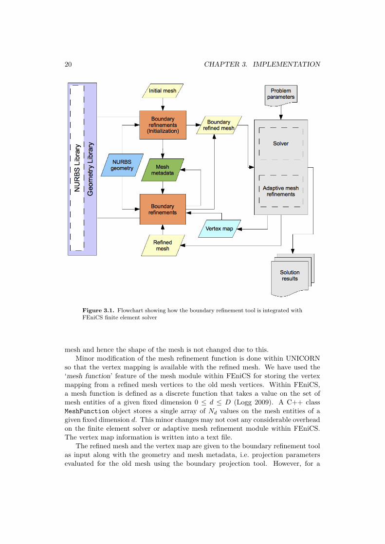
Figure 3.1. Flowchart showing how the boundary refinement tool is integrated withFEniCS finite element solver

mesh and hence the shape of the mesh is not changed due to this.Minor modification of the mesh refinement function is done within UNICORN

so that the vertex mapping is available with the refined mesh. We have used the‘mesh function’ feature of the mesh module within FEniCS for storing the vertexmapping from a refined mesh vertices to the old mesh vertices. Within FEniCS,a mesh function is defined as a discrete function that takes a value on the set ofmesh entities of a given fixed dimension 0 ≤ d ≤ D (Logg 2009). A C++ classMeshFunction object stores a single array of Nd values on the mesh entities of agiven fixed dimension d. This minor changes may not cost any considerable overheadon the finite element solver or adaptive mesh refinement module within FEniCS.The vertex map information is written into a text file.

The refined mesh and the vertex map are given to the boundary refinement toolas input along with the geometry and mesh metadata, i.e. projection parametersevaluated for the old mesh using the boundary projection tool. However, for a

3.4. INTEGRATION WITH FENICS 21

newly created mesh a vertex map and mesh metadata are not available. In thatcase the initial mesh and the corresponding geometry are given to the boundaryprojection tool and the mesh metadata with the projection parameters is preparedfor use in the next iteration. Mesh functions of FEniCS have been used to storethe point projection parameters as well as the index of the NURBS curve segmentor surface patch with each boundary vertex of a mesh. For a point projection ona NURBS curve, a single projection parameter is stored for each vertex where fora point projection on a surface, two parameters are used and two mesh functionobjects are used for that purpose. The respective index of the NURBS are storedusing another mesh function object. The mesh functions are stored within text fileswhich are later used to project the new node parameters for the refined mesh.

Explicit checking for the development of inverted cell is done at the end of meshsmoothing to ensure the mesh is valid for finite element analysis. Once an invertedcell is found, the whole mesh is rejected.

3.4.2 Running the SystemsIn the current process flow for solving a problem using UNICORN, once a solver isconfigured, a mesh along with the required parameters are given as input. Basedon the given parameters the dual problems are solved using finite element methodand based on the dual solution and the residuals an a posteriori error estimate ismeasured. According to the a posteriori error estimate the mesh is refined and thenthe solver continues to perform the same cycle in the next iteration using the refinedmesh. The boundary smoothing tool is plugged in the process to perform after themesh is adaptively refined. Figure 3.1 shows the flow chart of the boundary refine-ment process (i.e. the boundary smoothing tool) integrated with the UNICORNfinite element solver. Once the boundary smoothing is performed the refined meshis fed back to the solver for the next iteration.

Chapter 4

Results

From the experimental results we see that the vertex repositioning based boundarysmoothing works practically well for the simple cases of 2D and 3D geometries. Westart with a very coarse mesh and apply mesh refinements along with the boundarysmoothing to show the effectiveness of the proposed technique.

(a) Initial coarse mesh (b) After one refinement (c) After five refinements

(d) After one refinementand boundary projections

(e) After two refinementsand boundary projections

(f) After five refinementsand boundary projections

Figure 4.1. Uniform mesh refinements for a circular cylinder in 2D using DOLFIN,(a) Shows the initial coarse mesh, the blue circle gives the exact geometry whichis approximated by the mesh, (b)-(c) Show the result of mesh refinements aroundthe body without boundary projections and (d)-(f) Show the mesh refinements withboundary projections

23

24 CHAPTER 4. RESULTS

Figure 4.1 shows how the mesh is re-shaped near the geometric boundary asthe mesh is uniformly refined for the simple 2D cylinder case. In the figure (see4.1(b)-4.1(c)), we see that without the boundary smoothing during refinements, thecoarse initial mesh with coarse elements around the geometric boundary remains thesame shaped for the entire solution where the vertex repositioning based boundarysmoothing captures the geometry well as we see in the figure (see 4.1(d)-4.1(f)). Wesee that with five mesh refinements we achieved a much better approximation ofthe 2D cylinder geometry.

Figure 4.2 shows the vertex repositioning based boundary smoothing of curvedgeometry for a case of 2D NACA airfoil in the case of uniform mesh refinements.As we observe in the figure the curved geometry is captured much more accuratelyas the mesh is refined. Clearly we have more smoothing done in the front as wellas the rear parts of the airfoil where the the geometry is more curved than theupper and bottom parts of the airfoil. It is to be noted that, for the NACA airfoilgeometry representation we used total 38 NURBS curve segments. It is possible

(a) Initial coarse mesh (b) After one refinement (c) After five refinements

(d) Initial coarse mesh (e) After one refinement (f) After five refinements

(g) Initial coarse mesh (h) After one refinement (i) After five refinements

Figure 4.2. Uniform mesh refinements using DOLFIN and boundary points projec-tions for a NACA airfoil in 2D, (a)-(c) Whole airfoil, (d)-(f) Front part of the airfoil,(g)-(i) Rear part of the airfoil

4.1. PERFORMANCE 25

that a smaller number of curve segments can effectively represent the NACA air-foil, however, since the original source of the geometry were represented in Béziercurves, a direct conversion from Bézier curves to NURBS gave the 38 NURBS curvesegments. Please also note that, as neighbor information based point projection isnot implemented within this project, this projection is done using a search in allcurve segments, i.e. by discretizing parameter spaces of all the curve segments, for asingle point projection using Newton iteration. However, for the 2D cases, we havecomputationally much less expensive problem comparing to the 3D cases, henceperformance issues were not observed.

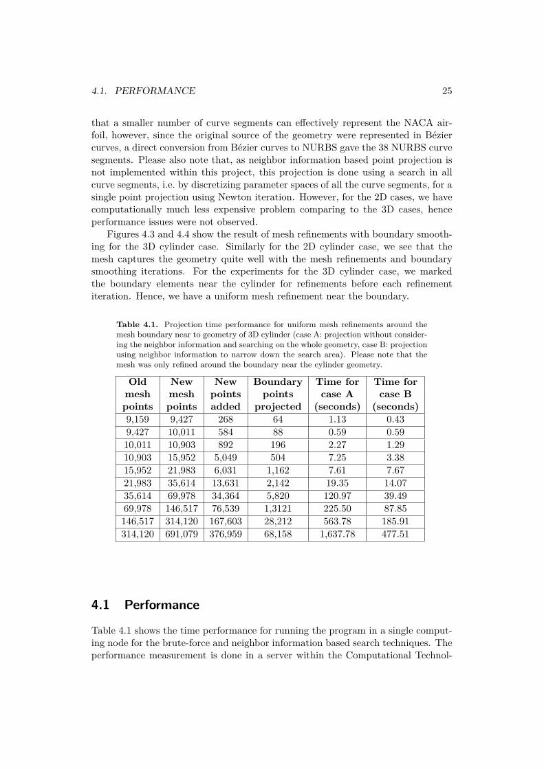
Figures 4.3 and 4.4 show the result of mesh refinements with boundary smooth-ing for the 3D cylinder case. Similarly for the 2D cylinder case, we see that themesh captures the geometry quite well with the mesh refinements and boundarysmoothing iterations. For the experiments for the 3D cylinder case, we markedthe boundary elements near the cylinder for refinements before each refinementiteration. Hence, we have a uniform mesh refinement near the boundary.

Table 4.1. Projection time performance for uniform mesh refinements around themesh boundary near to geometry of 3D cylinder (case A: projection without consider-ing the neighbor information and searching on the whole geometry, case B: projectionusing neighbor information to narrow down the search area). Please note that themesh was only refined around the boundary near the cylinder geometry.

Old New New Boundary Time for Time formesh mesh points points case A case Bpoints points added projected (seconds) (seconds)9,159 9,427 268 64 1.13 0.439,427 10,011 584 88 0.59 0.5910,011 10,903 892 196 2.27 1.2910,903 15,952 5,049 504 7.25 3.3815,952 21,983 6,031 1,162 7.61 7.6721,983 35,614 13,631 2,142 19.35 14.0735,614 69,978 34,364 5,820 120.97 39.4969,978 146,517 76,539 1,3121 225.50 87.85146,517 314,120 167,603 28,212 563.78 185.91314,120 691,079 376,959 68,158 1,637.78 477.51

4.1 Performance

Table 4.1 shows the time performance for running the program in a single comput-ing node for the brute-force and neighbor information based search techniques. Theperformance measurement is done in a server within the Computational Technol-


(a) Initial coarse mesh (b) 2 refinements (c) 4 refinements

(d) 6 refinements (e) 8 refinements (f) 10 refinements

Figure 4.3. Uniform mesh refinements around the surface boundary with boundaryprojections for a circular cylinder in 3D, (a) Initial coarse mesh, (b)-(f) Refined meshwith boundary projections

(a) Initial mesh (b) 2 refinements (c) 4 refinements (d) 6 refinements (e) 8 refinements

Figure 4.4. A different view on uniform mesh refinements around the surface bound-ary with boundary projections for a circular cylinder in 3D, (a) Initial coarse mesh,(b)-(e) Refined mesh with boundary projections

4.1. PERFORMANCE 27

Table 4.2. Distribution of iterations required for convergence for points projection ona 3D cylinder geometry. Maximum 1000 iterations allowed, hence, the frequencies inthe row of 1000 iterations apparently represents non-convergence (case A: projectionwithout considering the neighbor information and searching on the whole geometry,case B: projection using neighbor information to narrow down the search area)

Iterations Case A case Bcount frequency frequency1-5 11,802,941 12,066,1556-10 47,270 1211-15 1,606 016-20 296 021-25 100 026-30 10 031-35 30 036-999 0 01000 213,914 0Total 12,066,167 12,066,167

ogy Laboratory (CTL)1. The server has four Dual-Core AMD Opteron(tm) 2 GHzprocessors and overall 4.12 GB system memory. The system runs on Ubuntu Linux.The GNU C++ Compiler version 4.3 is used.

From the experimental results we found that the time requirements per iterationis approximately constant. For the test cases more than 95% of the iterations aredone within a range of 10-12 nano seconds. Given the iteration time is constant,one would be interested to play with the limit of maximum allowed iterations sincelimiting the maximum iterations within relatively small number would bound therunning time for each point projection for a given initial guess smaller.

We argue that it can be possible to limit the maximum iterations within fewtens of numbers (at least for simple cases such as 3D cylinder, etc.) as the table4.2 shows that for the point projection without neighbor information based searchmaximum iterations required are within 35 (34, to be exact) for successful cases andotherwise there are a considerable number of cases where 1000 iterations are used,which is the maximum allowed iterations for a projection search. We observe thatno projection required iterations from 35 to 999. We got support to believe thatif a point projection is not found within a sufficiently small number it is less likelythat we will reach the solution within finite number of iterations. This is becausethe Newton iterations are good for searching local optima and very sensitive to theinitial guess.

From the other case where neighbor node information is used to narrow down thesearch area, we find the performance is much better as we see in table 4.2. For thiscase, actually a maximum of 7 iterations were required for 12 point projection cases.

1Computational Technology Laboratory WWW link: http://ctl.csc.kth.se/


The technique improved the point projection search since this makes the Newtoniteration to search within sufficiently local region. In this case only a maximumseven iterations are used by all the 1.2066167 × 107 cases. Moreover, most of theprojections are reached within only two iterations.

Once we set the maximum allowed iterations to a sufficiently low number, timeper search with each initial guess will be bounded and we would be interested inminimizing discretization points of the narrowed down search area.

Figure 4.5. Cell quality based on affine cell mapping to a reference cell for the3D cylinder after the mesh refinements and boundary projections. Adaptive meshrefinements in UNICORN based on the dual solution is used for the refinements.

4.2 Mesh QualityAvoiding inverted cells is a must have requirement for a finite element mesh. Thereare other features a quality mesh should have. A quality mesh is very importantin finite element analysis since a mesh without sufficient quality may negativelyimpact on the accuracy and the efficiency of the solution. Knupp (2007) discussedabout mesh quality in the context of both finite difference and finite element meth-ods. Although Knupp (2007) emphasized on underlying problem oriented qualitymeasurements, in this thesis we focus on mesh quality measurement independent ofthe problem, rather based on the available mesh only.

Boundary smoothing using point projection based on the neighbor informationsuccessfully avoided creation of any inverted cell for the test cases discussed in this

4.3. BOUNDARY SMOOTHING WITH ADAPTIVE REFINEMENTS 29

thesis. We have used 10 × 10 discretization points in the parameter space of thetrimmed region for the 3D case.

UNICORN has been used to measure the cell quality where the mean-ratiometric (see Diachin et al. 2006) is implemented. Here the cell quality qe can havea range of values 0 < qe ≤ 1 with qe = 1 only when the element attains the idealreference shape. Figure 4.5 shows the cell quality after boundary smoothing afterthe mesh is refined around the boundary for the 3D cylinder case. The diffusion ofthe cell quality distribution from the initial mesh was as expected and we do notsee the algorithm to have any major impact on the mesh quality.

Radius ratio based cell quality measurement also shows that the boundarysmoothing done well in maintaining the cell quality as starting the the coarse meshand applying 20 adaptive mesh refinements iterations gives a maximum radius ratio2.1437 when boundary smoothing is not done and on the other hand using boundarysmoothing the radius ratio is 1.9246. Also after 25 adaptive iterations the valuesare 2.1436 and 1.9563 respectively. Surprisingly in these two cases using the ver-tex repositioning based boundary smoothing along with the refinements performedbetter than the refinements without boundary smoothing. However, please notethat in the boundary smoothing tool the internal mesh is smoothed as well whichhelps the mesh quality. We also note that the mesh refinements for this geometrywithout boundary smoothing gives a more stable radius ratio than using boundarysmoothing as for the case after 10 refinements the values are respectively 2.1437 and2.5301 where the cell quality result is favored to the non-boundary smoothing case.However, the mesh here had a very rough approximation of the 2D cylinder thatshould have helped the mesh refinement without boundary smoothing to maintaina fixed cell quality as the cells near the curved geometry are often irregular than acoarse linear approximation of the geometry.

4.3 Boundary Smoothing with Adaptive Refinements

Figure 4.6 shows the mesh refinement iterations using adaptive mesh refinementfeatures available in UNICORN based on an a posteriori error estimates. From thefigure we see that the mesh refinements is not uniform around the geometry. Thisis what one should expect from adaptive mesh refinements. However, we see thatdue to this reason the boundary smoothing is not uniform either and it took quitea few adaptive refinements iterations to obtain a shape of the mesh which capturesthe geometry better. However, we once observe more closely, we may see thatcomparatively larger mesh elements are available on the rear end of the cylinderand that causes more linear shape of the mesh. We emphasize that such elementswill eventually be refined if the mesh is adaptively more refined and as the meshwill be refined the vertex repositioning based boundary smoothing technique willuse the increased degree of freedom to capture the geometry better.

Adaptive mesh refinements based on an a posteriori error estimate using dualsolutions refines a percent of the mesh elements which is often non-uniformly dis-


(a) Initial mesh (b) 1 refinement (c) 2 refinements

(d) 3 refinements (e) 4 refinements (f) 5 refinements

(g) 6 refinements (h) 7 refinements (i) 8 refinements

Figure 4.6. Adaptive mesh refinements based on the solution of the dual velocityproblem using the dual solver provided by UNICORN. Boundary projections are donefor boundary smoothing after each refinements by adaptive refinements. It took afew iterations step to the mesh to capture the geometry of the circular cylinder quitewell due to non-uniform mesh refinements around the body of the geometry. Plotsshow the dual velocity solution and the corresponding mesh.

4.3. BOUNDARY SMOOTHING WITH ADAPTIVE REFINEMENTS 31

(a) Mesh with rough geometry (b) Mesh closer to the geometric shape

Figure 4.7. Differences in flow streamlines due to differences in geometric shape ofthe mesh, (a) Shows how the streamlines going through a region which is actuallyinside the cylinder which is outside of the domain, (b) Shows how a better mesh, thatcaptures the geometry better, gives an improved solution.

tributed. In that case the cells refinements around the geometry is not uniform andwhich causes elements of different sizes around the geometry. This is often problemspecific since for a flow past a cylinder problem one would expect that the meshelements above and below of cylinder are finer than the elements in the front andrear parts of the cylinder (flow is from the left) as we observe in the figure 4.6 for the2D cylinder case. In the figure we see that some elements near the cylinder body aremuch larger comparing to other elements. Such larger elements cause sharp edgessince if there are not enough number of mesh points near the boundary the curvedshape of the geometry may not be captured.

Figure 4.7 shows the changes in the streamlines near the curved boundary of thegeometry in the case of 3D cylinder. As we expect the coarse mesh that capturesthe geometry roughly, results wrong path of the streamlines which apparently gothrough the cylinder, i.e. the flow goes through the outside of the domain. Oncethe mesh is refined with boundary smoothing we get a better result.

Chapter 5

Conclusion

In this thesis we have presented a vertex repositioning based boundary smoothingtechnique for the finite element mesh. Experimental results show that using theproposed technique it is sufficient to start with a coarse mesh all over the domainand adaptively refine the mesh and the coarse mesh, as refined, captures the curvedgeometry more accurately.

In the proposed technique, the boundary vertices are repositioned on the geom-etry and the shape of the mesh captures the geometric shape of the domain witha higher accuracy as the mesh is refined. Newton iteration based iterative closestpoint search algorithms have been used to search point projection of a vertex on tothe CAD geometry represented in NURBS curves (2D) or surfaces (3D). A techniqueis proposed for obtaining sufficiently accurate initial guess region which is narrowenough comparing to the whole geometry. Once a mesh is refined the new boundaryvertices are projected on to the geometry using neighbor nodes’ projection data forobtaining more accurate initial guess for the Newton iteration. Projection param-eters for the original coarse mesh are gathered for a single time using exhaustivesearch for points projection on the whole geometry.

Experimental results show that the method is sufficiently accurate and efficientfor both 2D and 3D problems for some simple test cases. The process of boundarysmoothing takes a minor fraction of time in comparison to the finite element solutionand adaptive mesh refinements in the sense that the boundary smoothing is donewithin seconds to minutes where the solver runs for hours to days.

Since our techniques does not change the mesh topology and the finite elementsolver or mesh elements are not required to be changed, the developed tools canbe plugged in to the finite element solver without much involvements. Althoughthe tools are developed to be integrated parts of FEniCS applications, the parts ofgeometric data manipulation can be used with other applications as well.

33

34 CHAPTER 5. CONCLUSION

5.1 Future WorksIn this thesis we have considered orthogonal point projection for vertex reposition-ing. However, orthogonal point projection may sometimes result thin elements.This is within the scope of future improvements to consider other projections wherean investigation on orthogonal and other projection techniques will be required.

One major missing feature is that we did not consider the trimmed NURBS.Trimmed NURBS are often necessary in CAD since it is a well-used tool when two ormore NURBS patches are attached. In CAD using NURBS often one may encounterdifficulties to represent a surface using NURBS due to is rectangular definition.Trimmed surfaces are commonly used to overcome such difficulties. A trimmedsurface is an ordinary tensor product surface along with a restricted parameterdomain which is given by a trimming curve (Casciola & Morigi 1999). Efremov(2004) described an algorithm for ‘trimming test’ which effectively identifies whethera point on a NURBS surface patch lies within the trimmed region. Sederberg et al.(2008) discussed on the problems of having gaps when two NURBS surfaces areattached using trimmed NURBS method and proposed a resolution for that.

Within our application, if a projected point on a NURBS surface lies within thetrimmed region, the point projection has to be rejected since the trimmed region ofa NURBS surface does not represent the outer surface boundary of a finite elementmesh. Also, our implementation does not support geometry with multiple NURBScurves or patches. A natural continuation of this project may be to remove thelimitations by considering the cases where a surface geometry contains multipleNURBS patches connected at the edges or using trimmed NURBS.

The initial projection is done using brute-force technique in this thesis. Al-though, it is to be used once with the initial mesh to prepare the mesh metadatafor the boundary projections, one would be interested to improve the algorithm byusing some search heuristics.

Bibliography

Angel, E. (1999), Interactive Computer Graphics: A Top-Down Approach withOpenGL, 2nd edn, Addison-Wesley.

Bazilevs, Y., Zhang, Y., Calo, V. M., Goswami, S., Bajaj, C. L. & Hughes, T. J.(2006), ‘Isogeometric analysis of blood flow: a NURBS-based approach’, Com-pIMAGE, Coimbra, Portugal pp. 20–21.

Boyd, S. & Vandenberghe, L. (2004), Convex Optimization, Cambridge UniversityPress.

Casciola, G. & Morigi, S. (1999), The trimmed NURBS age, in ‘Advances in Com-putation: Theory and Practice; Recent Trends in Numerical Analysis’.

Chen, X.-D., Su, H., Yong, J.-H., Paul, J.-C. & Sun, J.-G. (2007), ‘A counterex-ample on point inversion and projection for NURBS curve’, Computer AidedGeometric Design 24(5), 302.

Chen, X.-D., Xu, G., Yong, J.-H., Yong, J.-H. & Paul, J.-C. (2009), ‘Computing theminimum distance between a point and a clamped B-spline surface’, GraphicalModels 71(3), 107–112.

Chen, X.-D., Yong, J.-H., Wang, G., Paul, J.-C. & Xu, G. (2008), ‘Computing theminimum distance between a point and a NURBS curve’, Computer-Aided Design40, 1051–1054.

Chou, J. J. & Logan, M. A. (1995), NASA-IGES translator and viewer, TechnicalReport 19950022354, NASA, USA.

Cottrell, J. (2007), Isogeometric Analysis and Numerical Modeling of the Fine Scaleswithin the Variational Multiscale Method, PhD thesis, The University of Texasat Austin, USA.

de Boor, C. (1972), ‘On calculating with B-splines’, Journal of Approximation The-ory 6, 50–62.

Diachin, L. F., Knupp, P., Munson, T. & Shontz, S. (2006), ‘A comparison of twooptimization methods for mesh quality improvement’, Engineering with Comput-ers 22(2), 61–74.

35

36 BIBLIOGRAPHY

Dyllong, E. & Luther, W. (1999), Distance calculation between a point and aNURBS surface, in P.-J. Laurent, P. Sablonnitre & L. L. Schurnaker, eds, ‘Curveand Surface Design’, pp. 55–62.

Efremov, A. (2004), Efficient ray tracing of trimmed NURBS surfaces, Master’s the-sis, University of Saarland, Computer Science Department, Max-Planck-Institutfur Informatik, Computer Graphics Group, Saarbrucken, Germany.

Elber, G. & Kim, M.-S. (2001), Geometric constraint solver using multivariate ra-tional spline functions, in ‘SMA ’01: Proceedings of the sixth ACM symposiumon Solid modeling and applications’, ACM, New York, NY, USA, pp. 1–10.

Eriksson, K., Estep, D., Hansbo, P. & Johnson, C. (1996), Computational Differen-tial Equations, 2nd edn, Cambridge University Press.

FEniCS (2009), ‘FEniCS project’.URL: http://www.fenics.org/

Foley, J. D., van Dam, A., Feiner, S. K. & Hughes, J. F. (1995), Computer GraphicsPrinciples and Practice, 2nd edn, Addison-Wesley Professional.

Hoffman, J. (2009), ‘Efficient computation of mean drag for the subcritical flowpast a circular cylinder using general Galerkin G2’, International Journal forNumerical Methods in Fluids 59(11), 1241–1258.

Hoffman, J., Jansson, J., Jansson, N., Nazarov, M. & Stöckli, M. (2009), ‘UNI-CORN’.URL: http://www.fenics.org/wiki/Unicorn

Hughes, T. J. R., Cottrell, J. A. & Bazilevs, Y. (2005), ‘Isogeometric analysis:CAD, finite elements, NURBS, exact geometry and mesh refinement’, ComputerMethods in Applied Mechanics and Engineering 194(39–41), 4135–4195.

Johnson, D. E. & Cohen, E. (2005), Distance extrema for spline models usingtangent cones, in ‘Proceedings of Graphics Interface 2005’, Vol. 112, CanadianHuman-Computer Communications Society, Ontario, Canada, pp. 169–175.

Kitware (2009), ‘Pareview’.URL: http://www.paraview.org/

Knupp, P. M. (2007), Remarks on mesh quality, in ‘45th AIAA Aerospace SciencesMeeting and Exhibit’, Sandia National Laboratories, New Mexico, USA.

Lavoie, P. (1999), An introduction to NURBS++.URL: http://libnurbs.sourceforge.net/user.pdf

Lavoie, P. (2002), ‘The NURBS++ library’.URL: http://libnurbs.sourceforge.net/index.shtml

BIBLIOGRAPHY 37

Liu, X.-M., Yang, L., Yong, J.-H., Gu, H.-J. & Sun, J.-G. (2009), ‘A torus patchapproximation approach for point projection on surfaces’, Computer Aided Geo-metric Design 26(5), 593–598.

Logg, A. (2009), ‘Efficient representation of computational meshes’, InternationalJournal of Computational Science and Engineering .

Logg, A., Wells, G. N. et al. (2009), ‘DOLFIN’.URL: http://www.fenics.org/dolfin/

Ma, Y. L. & Hewitt, W. T. (2003), ‘Point inversion and projection for nurbscurve and surface: Control polygon approach’, Computer Aided Geometric Design20(2), 79–99.

Piegl, L. A. & Tiller, W. (1996), The NURBS Book, 2nd edn, Springer.

Piegl, L. A. & Tiller, W. (2001), ‘Parametrization for surface fitting in reverseengineering’, Computer-Aided Design 33(8), 593–603.

Schroeder, W., Martin, K. & Lorensen, B. (2006), Visualization Toolkit: An Object-Oriented Approach to 3D Graphics, 4th edn, Kitware.

Sederberg, T. W., Li, X., Lin, H. & Ipson, H. (2008), ‘Watertight trimmed NURBS’,ACM Transactions on Graphics 27(3), 1–8.

Sevilla, R. (2009), NURBS-Enhanced Finite Element Method (NEFEM), PhD the-sis, Polytechnic University of Catalonia, Barcelona, Spain.URL: http://www-lacan.upc.edu/sevilla/webNEFEM.html

Sevilla, R., Fernández-Méndez, S. & Huerta, A. (2008), ‘NURBS-enhanced finiteelement method (NEFEM)’, International Journal for Numerical Methods in En-gineering 76(1), 56–83.

Smith, B. M. (1983), ‘IGES: A key to CAD/CAM systems integration’, IEEE Com-puter Graphics and Applications 3(8), 78–83.

Thompson, J. F., Soni, B. K. & Weatherill, N. P., eds (1998), Handbook of GridGeneration, 1st edn, CRC-Press.

US PRO (1996), The Initial Graphics Exchange Specification (IGES), 5.3 edn,IGES/PDES Organization.

Xu, J., Liu, W., Bian, H. & Li, L. (2008), ‘Accurate and efficient algorithm forthe closest point on a parametric curve’, International Conference on ComputerScience and Software Engineering .

Zhou, J., Sherbrooke, E. C. & Patrikalakis, N. M. (1993), ‘Computation of station-ary points of distance functions’, Engineering with Computers 9(4), 231–246.

38 BIBLIOGRAPHY

Zhou, X. & Lu, J. (2005), NURBS-based Galerkin method and application to skele-tal muscle modeling, in ‘Proceedings of the 2005 ACM symposium on Solid andphysical modeling’, pp. 71–78.

Appendix A

Introduction to Curves and Surfaces

There are three ways commonly used to model curves and surfaces, i.e. the ex-plicit equations, implicit equations and parametric functions. Implicit equationsand parametric functions are the two most commonly used methods of represent-ing curves and surfaces in geometric modeling. NURBS (Non-Uniform RationalB-Spline) are categorized within the parametric functions. We consider NURBS asthe geometric representation within the thesis. However, we will give brief introduc-tion to other representations to motivate the choice of representation. Other thanthe reason that NURBS are widely used in the CAD industries, NURBS also offersenhanced flexibility and precision for handling both analytic and freeform shapes.We will give a brief introduction to the three forms below. We refer to Angel (1999),Foley et al. (1995), Piegl & Tiller (1996) for the details on curves and surfaces.

A.1 Explicit equationsThe explicit form of a curve in two dimensions gives the value of one variable thedependent variable, in terms of the other, the independent variable. In the twodimensional x, y-space we have the explicit equations of the following form

y = f(x)

where x is the dependent variable and y is the independent variable and they areconnected using the function f . Sometimes it is possible to find the invert relationsof the form, x = g(y).

In three dimensions, a surface is represented using one equation of the form

z = f(x, y)

where we have two independent variables x, y and one dependent variable z, whiletwo equations are required to represent a curve{

y = f(x)z = g(x)

39

40 APPENDIX A. INTRODUCTION TO CURVES AND SURFACES

where we have one independent variable x and two dependent variables y and z.A major disadvantage of the explicit form of geometry representation is that we

don’t have guarantee that either form exists for a given curve. For example, fora line represented in the form y = mx + c where m is the slope of the line and cis the y-intercept, we cannot represent a vertical line. Also to represent a simplecircle we require two explicit equations for different parts of it. Another exampleis for a circle where we require two equations for different parts of it, i.e. usingexplicit representation we can write the equation for half of it, y =

√r2 − x2 and

write another equation for the second half. Here, r is the radius of the circle withcenter at the origin. Similarly, for a line in the three dimension defined using twoequations (y = ax+ b and z = cx+ d) would fail to represent a line with constant xand a surface represented by an equation of the form z = f(x, y) cannot representa sphere since we would require two z points for a given x and y pair which is notdefined in such form of equations.

A.2 Implicit equationsImplicit equation of a curve in two dimensional xy plane has the form

f(x, y) = 0

describing an implicit relationship between the x and y coordinates of the pointslying on the curve and a surface in the three dimension is defined by an implicitequation has the form

f(x, y, z) = 0

For example, a straight line in implicit representation has the form, ax+ by+ c = 0where a circle, with the center in the origin and radius r, can be represented asx2 + y2− r2 = 0 and a plane in 3D can be represented as ax+ by+ cz+d = 0. Herea, b, c and d are constants. A sphere with the center at the origin can be written as,x2 + y2 + z2 − r2 = 0. Such an implicit equation describes the implicit relationshipbetween the x, y and z coordinates of the points lying on the curve or surface.

Using the implicit representation we test the points (xi, yi) to know whether thepoint is on the curve or not. We can take a point (x, y) and evaluate f to determinewhether the point lies on the curve.

Although, most of the curves and surfaces with which we work have implicitrepresentations (Angel 1999), in general, however, it gives us no analytic way tofind a value y on the curve the corresponds to a given x, or vice versa. However, theimplicit form is less dependent on the coordinate systems than the explicit form,hence, it is possible to represent all lines and circles using the implicit representa-tions.

Another disadvantage is that curves in three dimensions are not as easily rep-resented in implicit form. We require to represent a curve as the intersection, if it

A.3. PARAMETRIC FUNCTIONS 41

exists, of the two surfaces: {f(x, y, z) = 0g(x, y, z) = 0

Then we test if a point (x, y, z) lies on both the surfaces and in that case we knowthat it must lie on their intersection curve.

A.3 Parametric functionsIn the parametric form of a curve the spatial variables for the points on the curveis defined in terms of an independent variable u where u is called the parameter. In2D the we have two explicit functions

x = x(u), y = y(u)

where in 3D we have

x = x(u), y = y(u), z = z(u)

One of the advantages of the parametric form is that we simply drop the equa-tion for z from the three dimensional representation to obtain the two dimensionalrepresentation. In this sense, the parametric form is the same in two and threedimensions.

Using parametric functions we have the definition of the curve in two dimensionalplane as

C(u) = (x(u), y(u)), a ≤ u ≤ b

where a, b are arbitrary constants (usually normalized to [0, 1]). Here, C is a vector-valued function of the independent variable u. It is common to think of C(u) =(x(u), y(u)) as the path traced out by a particle as a function of time where u isthe time variable and [a, b] is the time interval.

A surface in the parametric representation is defined as

S(u, v) = (x(u, v), y(u, v), z(u, v)), a ≤ u ≤ b, c ≤ v ≤ d

As we see that we require two independent variables u and v to define a surface inthe parametric representation.

For example, the first quadrant of a unit circle can be defined using the para-metric functions

C(u) = (x(u), y(u)) = (cos(u), sin(u))T , 0 ≤ u ≤ π/2

or alternatively using t = tan(u/2), we can represent the same curve using

C(t) = (x(t), y(t)) =(

1− t21 + t2

,2t

1 + t2

)T, 0 ≤ t ≤ 1


A sphere in 3D can be defined in parametric representation as

S(u, v) = (x(u, v), y(u, v), z(u, v))T = (sin u cosu, sin u sin v, cosu)T (A.1)

where 0 ≤ u ≤ π and 0 ≤ v ≤ 2π. From the above representation of the sphere wesee that two independent variables u and v are required to define a surface. Holdingu fixed and varying v generates the latitudinal lines of the sphere and on the otherhand holding v fixed and varying u generates the longitudinal lines.

As we have observed for the circle’s representation above, parametric repre-sentation of the sphere is not unique. Parametric forms of curves and surfacesrepresentations are not unique. Similarly, any given curve or surface can be repre-sented in different ways. Actually, the representation can be different and differentrepresentations have different benefits and disadvantages and one should carefullyselect the appropriate representation of the CAD model based on the requirementsof the applications.

For the coordinate system related difficulties and non-existence of the repre-sentation (although the curve or surface exists, the representation is not available),explicit equations are not generally suitable for using in computer graphics and com-puter aided designing. Implicit and parametric functions are the two most commonmethods of representing curves and surfaces in geometric modeling. As we willsee in the following discussions, there are different representations available withinparametric functions.

The parametric form of curves and surfaces is the most flexible and robust incomputer graphics, although one could still argue that we have not fully removedall dependencies on a particular coordinate system or frame as we are still using thex, y and z for a particular representation (Angel 1999).

In the paremetric forms in which the functions are polynomials in u for curves,and polynomials in u and v for surfaces, are of most use in computer graphics(Angel 1999). Such forms are called as the parametric polynomial forms of curvesand surfaces representation.

NURBS for external data storage and more sophisticated geometry definition.Other representations are mainly for internal use to take advantages of differentfeatures that would be important for computations.

A.3.1 Parametric Polynomial Curves

We consider a curve of the form

p(u) = (x(u), y(u), z(u))T

Then a polynomial parametric curve of degree n is of the form

p(u) =n∑k=0

ukck

A.3. PARAMETRIC FUNCTIONS 43

where each ck = (cxk, cyk, czk)T has independent x, y and z components. Here then + 1 column matrices {ck} are the coefficients of p, which clearly gives 3(n + 1)degrees of freedom in how we choose the coefficients of a particular p.

An interesting properties of polynomial curves is that there is no coupling,among the x, y, and z components and this allows us to work with three inde-pendent equations, each of the form

p(u) =n∑k=0

ukck

and each with n + 1 degrees of freedom. Although u can be defined for any rangeumin ≤ u ≤ umax, it is a common practice to consider 0 ≤ u ≤ 1.

Polynomials are classified within a widely used class of functions. In this sectionwe will introduce a few methods of expressing polynomial functions. Althoughthey are mathematically equivalent, some of the representations are better than theothers in the terms of computer representations and manipulations.

Degree of a parametric polynomial curve must be chosen carefully which isdependent on the applications. Choosing a high degree will give us many parametersto control, i.e. increased flexibility and control over the shape of the curve, butevaluation of points on the curve will be costly. Also there is more danger that thecurve will become rougher as the degree of a polynomial curve becomes higher. Onthe other hand, choosing too low a degree, we may not have enough parametersand we may require to design each curve segment only over a short interval. Cubicpolynomials are most often used due to insufficient flexibility in controlling theshape of the curve using lower-degree polynomials and higher-degree polynomialscan introduce unwanted wiggles and can be computationally expensive. However, itis noted that, although higher-degrees curves require more conditions to determinethe coefficients and can wiggle back and forth in ways that are difficult to control,they are used in applications– such as the design of cars and planes– in which higher-degree derivatives must be controlled to create surface that are aerodynamicallyefficient.

An nth degree power basis curve is given by

p(u) = (x(u), y(u), z(u))T =n∑i=0

aiui, 0 ≤ u ≤ 1 (A.2)

where ai = (xi, yi, zi) are vectors, hence

x(u) =n∑i=0

xiui, y(u) =

n∑i=0

yiui, z(u) =

n∑i=0

ziui

Equation (A.2) can be written in matrix form as

p(u) =[a0 a1 · · · an

] [1 u u2 · · · un

]T= [ai]T [ui]


Here, the n+1 functions {ui} are called the basis functions (or blending functions).A parametric cubic polynomial curve is a special case of the power basis form

of a curve where we have n = 3. A cubic parametric polynomial can be given as

p(u) = a0 + a1u+ a2u2 + a3u

3 =3∑i=0

aiui

Two prominent examples of cubic polynomial curve representations are Her-mite and Bézier representations. The Hermite form of the cubic polynomial curvesegment is determined by constraints on the endpoints and tangent vectors at theendpoints, where the Bézier form of the cubic polynomial curve segment is deter-mined by constraints on the endpoints and two intermediate points that, along withthe endpoints, specify the tangent vectors at the endpoints.

A.3.2 Parametric Polynomial SurfacesA parametric polynomial surface can be defined as

p(u, v) = (x(u, v), y(u, v), z(u, v))T =n∑i=0

m∑j=0

cijuivj

Here we require to specify 3(n + 1)(m + 1) coefficients to determine a particularsurface p(u, v). This is common practice to take n = m, and let u and v vary overthe rectangle 0 ≤ u, v ≤ 1, defining a surface patch. Please note that any surfacepatch can be viewed as the limit of collection of curves that are generated by holdingeither u or v constant and varying the other.

A.4 B-Spline Basis FunctionsLet U = {u0, . . . , um} be a nondecreasing sequence of real numbers (i.e. ui ≤ui+1, i = 0, . . . ,m − 1). Then the ith B-spline basis function of p-degree, denotedby Ni,p(u), is recursively defined as

Ni,p(u) = u− uiui+p − ui

Ni,p−1(u) + ui+p+1 − uui+p+1 − ui+1

Ni+1,p−1(u) (A.3)

where the base case is defined as

Ni,0(u) ={

1 if ui ≤ u ≤ ui+10 otherwise

Here, ui is called ‘knots’ and U is the ‘knot vector’. The recurrence formula todefine the B-spline basis functions is the most useful for computer implementationand also widely used within computational geometry.

Although Ni,p(u), which are piecewise polynomials, are defined on the entirereal line, generally only the interval [u0, um] is of interest. The B-spline basis func-tions has local support, i.e. each Ni,p(u) is nonzero only on a limited number of

A.4. B-SPLINE BASIS FUNCTIONS 45

subintervals, not the entire domain, [u0, um]. Ni,p(u) = 0 if u is outside the interval[ui, ui+p+1). Clearly, in any given knot span, [uj , uj+1), at most p + 1 of the Ni,pare nonzero, namely the functions Nj−p,p, . . . , Nj,p. The B-spline basis functions arenonnegative, i.e. Ni,p(u) ≥ 0, ∀i, p, u.

A.4.1 B-Spline Curves

A pth-degree B-spline curve is defined by

C(u) =n∑i=0

Ni,p(u)Pi, a ≤ u ≤ b

where {Pi} are the ‘control points’, and the {Ni,p(u)} are the pth-degree B-splinebasis functions defined on non-periodic (and non-uniform) knot vector,

U = {a, . . . , a︸︷︷︸p+1

, up+1, . . . , um−p−1, b, . . . , b︸︷︷︸p+1

},

with a total m+ 1 knots. The polygon formed by the control points {Pi} is calledthe ‘control polygon’. The steps to compute a point on a B-spline curve is fairlystraightforward. At a fixed u value, first we require to find the knot span in whichu lies and compute the nonzero basis functions and finally we multiply the values ofthe nonzero basis functions with the corresponding control points. de Boor (1972)gave an efficient way of evaluating B-spline basis functions. Based on de Boor’s(1972) discussions Piegl & Tiller (1996) formulated the algorithms for finding theknot span and computing the nonzero basis functions and also the properties of theB-spline curves.

C(u) is a piecewise polynomial curve (since the Ni,p(u) are piecewise polynomi-als) where the degree, p, the number of control points, n + 1, and the number ofknots, m + 1, related by the relation: m = n + p + 1. The control polygon of theB-spline curve can be taken as a piecewise linear approximation to the curve andthe approximation is improved by knot insertion or degree elevation (see Piegl &Tiller 1996). As a general rule, the lower the degree, the closer a B-spline curvefollows its control polygon. This is because, the lower the degree, the fewer thecontrol points that are contributing to the computation of C(uk) for any given uk.In the extreme case where p = 1 we find the curve C(u) just by taking a linearinterpolation between two control points. In that case, the curve is actually thecontrol polygon. Another special case is if n = p and U = {0, . . . , 0, 1 . . . , 1}, thenC(u) is a Bézier curve.

A.4.2 B-Spline Surfaces

A B-spline surface is obtained by taking a bidirectional net of control points, twoknot vectors, and the products of the univariate B-spline basis functions. A B-spline


surface, constructed as tensor product of two B-spline curves, is defined by

S(u, v) =n∑i=0

m∑j=0

Ni,p(u)Nj,q(v)Pi,j , a ≤ u ≤ b, c ≤ v ≤ d

where {Pi,j} are the control points forming the control net, and the {Ni,p(u)} arethe pth-degree B-spline basis functions in the direction of U knot vector and the{Nj,q(v)} are the qth-degree B-spline basis functions in the direction of V knotvector defined on non-periodic (and non-uniform) knot vectors,

U = {a, . . . , a︸︷︷︸p+1

, up+1, . . . , ur−p−1, b, . . . , b︸︷︷︸p+1

}, V = {c, . . . , c︸︷︷︸q+1

, vq+1, . . . , vs−q−1, d, . . . , d︸︷︷︸q+1

}.

Here U has r + 1 knots and V has s + 1 with the relations: r = n + p + 1 ands = m+ q + 1.

A.5 NURBSNon-Uniform Rational B-Spline (NURBS) curves and surfaces are widely used forcomputer-aided design, manufacturing and engineering industries for its advantagesover other representations.

A.5.1 NURBS CurvesA pth-degree NURBS curve is defined as

C(u) =∑ni=0Ni,p(u)wiPi∑ni=0Ni,p(u)wi

, a ≤ u ≤ b

where {Pi} are the control points, {wi} are the weights and {Ni,p(u)} are the pth-degree B-spline basis functions (equation (A.3)) defined on the non-periodic (andnon-uniform) knot vector

U = {a, . . . , a︸︷︷︸p+1

, up+1, . . . , , um−p−1 b, . . . , b︸︷︷︸p+1

}

Like the B-spline curves, the control points, {Pi}, forms the control polygon.The NURBS curves are often written in the following form

C(u) =n∑i=0

Ri,p(u)Pi

where

Ri,p(u) = Ni,p(u)wi∑nj=0Nj,p(u)wj

The {Ri,p(u)} are called the ‘rational basis functions’. They are piecewise rationalfunctions on u ∈ [0, 1].

A.6. DERIVATIVES OF PARAMETRIC CURVES AND SURFACES 47

A.5.2 NURBS Surfaces

A NURBS surface of degree p in the u direction and degree q in the v direction isdefined as

S(u, v) =∑ni=0

∑mj=0Ni,p(u)Nj,q(v)wi,jPi,j∑n

i=0∑mj=0Ni,p(u)Nj,q(v)wi,j

, a ≤ u ≤ b, c ≤ v ≤ d

Here S(u, v) is a bivariate vector-valued piecewise rational function. Here, {Pi,j}form a bidirectional control net, {wi,j} are weights and {Ni,p(u)} and {Nj,q(v)} arethe non-rational B-spline basis functions defined on the knot vectors,

U = {a, . . . , a︸︷︷︸p+1

, up+1, . . . , ur−p−1, b, . . . , b︸︷︷︸p+1

}, V = {c, . . . , c︸︷︷︸q+1

, vq+1, . . . , vs−q−1, d, . . . , d︸︷︷︸q+1

}.

Here U has r + 1 knots and V has s + 1 with the relations: r = n + p + 1 ands = m+ q + 1.

The NURBS surfaces are often written in the following form

S(u, v) =n∑i=0

m∑j=0

Ri,j(u, v)Pi,j

where

Ri,j(u, v) = Ni,p(u)Nj,q(u)wi,j∑nk=0

∑ml=0Nk,p(u)Nl,q(v)wk,l

are the piecewise rational basis functions.

A.6 Derivatives of parametric curves and surfacesFor the point projection and inversion on NURBS curves and surfaces algorithmsunder considerations in this thesis, we must evaluate the derivatives of NURBScurve. The first and second derivatives of parametric curves C(u) can be thoughtof the velocity and acceleration of the particle, respectively (Piegl & Tiller 1996).We refer to Piegl & Tiller (1996) for the details and evaluation of the derivatives ofNURBS curves and surfaces.

The first derivative of the parametric curve can be written in the form:

dC(u)du

=(dx(u)du

,dy(u)du

,dz(u)du

)TThe derivatives of parametric surface S(u, v), ∂S/∂u and ∂S/∂v

∂S(u, v)∂u

=(∂x(u, v)∂u

,∂y(u, v)∂u

,∂z(u, v)∂u

)T


and

∂S(u, v)∂v

=(∂x(u, v)∂v

,∂y(u, v)∂v

,∂z(u, v)∂v

)Tdetermine the tangent plane at each point of the surface. Here, ∂S/∂u and ∂S/∂vrespectively gives the velocities along latitudinal and longitudinal lines for the caseof the sphere.

The unit normal vector, N at any point on the surface is defined as below (Piegl& Tiller 1996)

N = Su × Sv|Su × Sv|

(A.4)

provided that the vector cross product Su × Sv does not vanish at the point. Aswe understand that there can be different parameterizations for the same surface,different parameterizations give different partial derivatives. However, the existenceof a normal vector at the point, and the corresponding tangent plane, is a geometricproperty of the surface independent of the parameterization. We will get the sameN in (A.4) independently of the parameterization provided that the denominatordoes not vanish.

However, it might be impossible to find the normal vector at some points ofthe surface in some parameterization even though the unit normal vector exists atthe point and can be obtained using a different parameterization. We illustratethis with an example taken from (Piegl & Tiller 1996). From equation (A.1) (anon-unique parameterization of a sphere), it can be seen that Sv(0, v) = Sv(π, v) =0,∀v, 0 ≤ v ≤ 2π, i.e., Sv vanishes at the north and south poles of the of the sphere.Although, normal vectors do exist at the two poles, we are unable to compute themusing equation (A.4) under this parameterization.

We note that, of the implicit and parametric forms, it is difficult to maintainthat one is always more appropriate than other. Both the representations havetheir advantages and disadvantages and a successful geometric modeling is doneusing both techniques (Piegl & Tiller 1996).

Appendix B

Point Projection on Curves and Surfaces

Piegl & Tiller (1996) discussed Newton’s iterations based straightforward algorithmsto solve point projection problem for NURBS curves and surfaces. The algorithmscan be categorized as the so called ‘iterative closest points’ algorithms or simplyICP. However, as it is common for any Newton’s iterations based algorithms, agood initial guess is required for the success of the algorithms which is the point tobe addressed for effective applications of these algorithms. In this chapter we givean overview of the algorithms and for the details discussions we refer to Piegl &Tiller (1996). Our techniques for obtaining sufficiently accurate initial guess for theNewton’s iterations are discussed in chapter 2.

Figure B.1. Points projection on a NURBS curve

49

50 APPENDIX B. POINT PROJECTION ON CURVES AND SURFACES

B.1 Point Projection on NURBS CurveLet’s assume that we have a initial guess u0 ∈ [umin, umax] and the minimum distancefrom a point P to the curve C(u) is found for u∗, i.e. ‖C(u)−P‖ = min{‖C(u)−P‖|u ∈ [umin, umax]}. Then the parameter u∗ that gives the minimum distance isfound by solving for f(u) = 0 where f(u) is defined as the form of the dot productfunction

f(u) = C′(u) · (C(u)−P)

Now, assuming the start value u0 and denoting by ui the parameter obtained at theith Newton iteration. Then

ui+1 = ui −f(ui)f ′(ui)

= ui −C′(ui) · (C(ui)−P)

C′′ · (C(ui)−P) + |C′(ui)|2(B.1)

Then the convergence criteria is given by the following inequalities where the con-vergence is reached if any of the following holds

1. If two points coincides, i.e. |C(ui)−P| ≤ ε1 or

2. The parameter does not change significantly, i.e.|(ui+1 − ui)C′(ui)| ≤ ε1 (this

may happen, for example, if the point is off the end of the curve) or

3. If zero cosine reached, i.e. |C′(ui) · (C(ui)−P)||C′(ui)||C(ui)−P| ≤ ε2.

If any of the above conditions is satisfied, the iterations are stopped and we reachedto the desired projection point. Otherwise we continue to iterations up to a largefinite number of times which we decide based on the problem using some heuristics.Here, to indicate convergence, two zero tolerances ε1 and ε2 are used as measure forEuclidian distance and zero cosine, respectively.

From the iteration equation (B.1) we see that there is no condition that willrestrict ui+1 from going outside the range umin ≤ ui+1 ≤ umax. To enforce the pa-rameter to stay within the range ui+1 ∈ [umin, umax] we require additional checkingon the new parameter (Piegl & Tiller 1996). If the curve is not closed, we simplyset ui+1 = umin if ui+1 < umin and ui+1 = umax if ui+1 > umax. If the curve is closedwe set ui+1 = umax− (umin−ui+1) and ui+1 = umin + (ui+1−umax) respectively forui+1 < umin and ui+1 > umax.

To obtain a start value, u0, for the Newton’s iterations, Piegl & Tiller (1996)suggested to evaluate the curve points at n equally spaced parameters values oneach candidate span, and compute the distance of each point from P. We requireto choose u0 to be the value yielding the point closest to P while the number n isgenerally chosen by some heuristic method.

Figure B.1 shows examples of point projection on a NURBS curve where theexternal given points stays on a circular path.

B.2. POINT PROJECTION ON NURBS SURFACE 51

B.2 Point Projection on NURBS SurfacePoint projection and inversion for NURBS surface are solved in similar way as forthe NURBS curve. Here we are given a NURBS surface S(u, v) and a point P andwe are interested to find a point on S(u, v) that minimizes the distance from P. Westart with defining the vector function r(u, v) as

r(u, v) = (S)(u, v)−P

Now we require r(u, v) to be orthogonal to the partial derivatives ∂S/∂u and ∂S/∂vand we define two scalar functions f(u, v) and g(u, v) as{

f(u, v) = r(u, v) · Su(u, v) = 0g(u, v) = r(u, v) · Sv(u, v) = 0 (B.2)

Solving the system (B.2) using an iterative method to obtain the parameters (ui, vi)gives the point on S(u, v) having minimum Euclidian distance from P.

Now, let

δi =[

∆u∆v

]=[ui+1 − uivi+1 − vi

]

Ji =[fu fvgu gv

]=[|Su|2 + r · Suu Su · Sv + r · Suv

Su · Sv + r · Svu |Sv|2 + r · Svv

]

κi = −[f(ui, vi)g(ui, vi)

]

Here, all the functions in the Jacobian matrix Ji are evaluated at (ui, vi). At the ithiteration we require to solve the simple 2× 2 system of linear equations, Jiδi = κi,to obtain the unknown δi which we use to obtain the parameter at next iterationtaking ui+1 = ui + ∆u and vi+1 = vi + ∆v.

Similar to the curve case, we have two zero tolerance parameters ε1 and ε2that are used respectively for point coincidence and zero cosine checking. Theconvergence criteria is given by the following inequalities where the convergence isreached if any of the following holds

1. If two points coincides, i.e. |S(ui, vi)−P| ≤ ε1 or

2. The parameter does not change significantly,i.e. |(ui+1 − ui)Su(ui, vi) + (vi+1 − vi)Sv(ui, vi)| ≤ ε1 or

3. If zero cosine reached,i.e. |Su(ui, vi) · (S(ui, vi)−P)|

|Su(ui, vi)||S(ui, vi)−P| ≤ ε2 and |Sv(ui, vi) · (S(ui, vi)−P)||Sv(ui, vi)||S(ui, vi)−P| ≤ ε2.

52 APPENDIX B. POINT PROJECTION ON CURVES AND SURFACES

If any of the convergence criteria is satisfied, the iterations are halted and we suc-cessfully reached to the desired projection point. Otherwise we continue to iterationsup to a maximum number of iterations.

We enforce the parameters to stay within the range umin ≤ ui+1 ≤ umax andvmin ≤ vi+1 ≤ vmax. If the surface is not closed in the u direction, we simplyset ui+1 = umin if ui+1 < umin and ui+1 = umax if ui+1 > umax, otherwise weset ui+1 = umax − (umin − ui+1) and ui+1 = umin + (ui+1 − umax) respectivelyfor ui+1 < umin and ui+1 > umax. Similarly, if the surface is not closed in the vdirection, we set vi+1 = vmin if vi+1 < vmin and vi+1 = vmax if vi+1 > vmax, otherwisewe set vi+1 = vmax − (vmin − vi+1) and vi+1 = vmin + (vi+1 − vmax) respectively forvi+1 < vmin and vi+1 > vmax.

Appendix C

IGES

Clearly the geometric CAD model is created using some external software and wewill require some import procedures to read the geometric data. There are severaldifferent available file formats; most CAD systems have their own file formats.However, there are a number of standard specifications that are developed andwidely adopted in the CAD industry, e.g. IGES, STEP, and PHIGS (see Piegl& Tiller 1996, ch 12). All of these specifications have their own advantages anddisadvantages and all are widely used. Many professional CAD software supportimport from and export to IGES, STEP, etc. formats.

The Initial Graphics Exchange Specification (IGES) (US PRO 1996) is one of theindustry standard data format specification for product design and manufacturinginformation. The information is generally created in a CAD/CAM system andstored for further use. IGES enables digital data exchange among CAD systemsby defining a neutral data format. This specification defines file structure andlanguage formats to represent geometric, topological, and non-geometric productdefinition data and these formats are independent of the modeling method used.Smith (1983) listed two benefits of this common format. First, a CAD/CAM systemdoes not require to have import and export systems for all the available data formatsavailable in the industry, which can be widely varied, rather one will only requireto develop systems for import from the IGES format CAD data file and export tosuch format. Second, ease in data storage in magnetic tape or disk and transmissionthrough telecommunications media. In today’s computing world, data storage andtransmission is far advanced than it was more than two decades ago, hence, thesecond reason for using IGES format can be ignored. However, the first reason isstill valid and even more important since today we have even more CAD systemsin the industry where most of them have their own data formats. In this project weare interested to the geometric data exchange in particular.

53

54 APPENDIX C. IGES

IGES File 1 2D CylinderDescription: Circle / Cylinder cross section (2D), NURBS S 1

Center = (0.2, 0.2, 0.0), Radius = 0.05 S 21H,,1H;,,,,,,,,,,,,1,4HINCH,,,,,,,,,,,; G 1

126 1 0 0 0 0 0 000000000D 1126 0 0 0 0 0D 2

126, 1P 18,2, 1P 21,1,0,0, 1P 30.0,0.0,0.0,0.25,0.25,0.5,0.5,0.75,0.75,1.0,1.0,1.0, 1P 41.0,0.707107,1.0,0.707107,1.0,0.707107,1.0,0.707107,1.0, 1P 50.25,0.2,0.0, 1P 60.25,0.25,0.0, 1P 70.2,0.25,0.0, 1P 80.15,0.25,0.0, 1P 90.15,0.2,0.0, 1P 100.15,0.15,0.0, 1P 110.2,0.15,0.0, 1P 120.25,0.15,0.0, 1P 130.25,0.2,0.0, 1P 140.0,1.0, 1P 150.0,0.0,1.0; 1P 16S 2G 1D 2P 16 T 1

C.1 File Format and Structure

A IGES specification file can be either an ASCII file or a binary file. ASCII formatfiles are more popular due to the flexibility that it can be easily modified usingany text editor. Two types of ASCII format files are used in IGES specifications;either in fixed or in compressed format. The compressed format file has not beenwidely implemented since commercial file compression software can reduce the sizeof fixed format files. In this thesis, we consider the ASCII fixed format files andthe other IGES files formats along with other standard data exchange specifications(e.g. STEP, etc.) are left for future considerations.

The fixed format files contain 80-character lines, grouped into sections. A sectionis identified by a letter code in column 73 of each line. The section specific datafields are available in the first 72 columns of each line and each section has ascendingsequence numbers, starting from 1, right justified (with leading space or zero filled)in columns 74-80. For a fixed format IGES specification file, the flag section is notrequired.

The IGES files have six sections that appear contiguously in the file (no blankline is allowed). The order of the sections are start section (S), global section (G),directory entry section (D), parameter data section (P) and terminate section (T).The directory entry and terminate sections contain data in fixed-length fields wherethe global and parameter data sections contain delimited, variable-length fields andthe start section is free from. IGES files 1 and 2 illustrates the structure of IGES

C.2. ENTITIES 55

for 2D and 3D cylinders respectively. Details of the file structure is available in USPRO (1996).

C.2 EntitiesWithin the IGES format file the fundamental unit of data is the ‘entity’; geometryentities define the physical shape of a product and include points, curves, surfaces,solids and relations that are collections of similarly structured entities and non-geometry entities specify associations among entities, etc. Since geometry entitiesgenerally are defined independently of one another, property and associativity enti-ties are used to augment and define their relationships. Each entity format includesits unique entity type and form numbers. In this thesis we are interested in geometryentities, and to be more specific, in NURBS curves and surfaces.

From the definition of the NURBS curve we see that we will require a knot vector,control points with corresponding weight information to describe a NURBS curve.The IGES specification of rational B-spline curves (entity type 126) gives theseinformation along with other required information (i.e. the degree of the curve andinformation about the number of control points, etc.) and additional information(e.g. curve is planner or not, if the curve is open or closed, etc.). A NURBS surfaceis also specified using similar data format. Within IGES specifications a B-splinesurface is identified by the entity type number 128.

C.2.1 Rational B-Spline Curve Entity (Type 126)Rational B-Spline curve entity may represent analytic curves of general interestand this is used to represent NURBS curves within this project. The form numbersfrom 0 through 5 are valid form numbers where we have opted the form number 0for our use where the form of the curve is determined from the rational B-splineparameters. We have not used the other form numbers which are used to representcurves form of lines and arcs of circular, elliptical, parabolic and hyperbolic shapes,respectively. Please note that using the form number preference 0 it is entirelypossible to represent these curve forms, however, the system is not aware of thespecial form of a curve in that case. For our applications, this does not make anydifficulty since our algorithms consider all the curves as generic NURBS curve.

As the NURBS curves are defined with knot sequences, control points and re-lated weight parameters, these information are available from the IGES specifica-tion of rational B-spline curve entity. There are other parameters available from thedefinition of a B-spline curve entity, some of which, depending on the system, areimportant parameters for the applications where some are for informational purposeonly. For our applications the parameter with the information that whether a curveis closed or open is used within our projection algorithm. A curve is consideredclosed if the beginning and ending points of the curve are coincident. The startingand ending points on the curve are defined by evaluating the curve at the start-ing and ending parameter values. Since the algorithms we are using are same for

56 APPENDIX C. IGES

planner/non-planner, rational/polynomial, periodic/non-periodic curves, we storethese information for informational purposes only.

IGES File 2 3D CylinderDescription: Cylinder (3D), NURBS S 1

Center(x,y)=(0.55, 0.5), zmin=0, zmax=0.4, Radius=0.05 S 21H,,1H;,,,,,,,,,,,,1,4HINCH,,,,,,,,,,,; G 1

128 1 0 0 0 0 0 000000000D 1128 0 0 0 0 0D 2

128, 1P 18,1,2,1, 1P 21,0,0,0,0, 1P 30.0,0.0,0.0,0.25,0.25,0.5,0.5,0.75,0.75,1.0,1.0,1.0, 1P 40,0,1,1, 1P 51.0,0.707107,1.0,0.707107,1.0,0.707107,1.0,0.707107,1.0, 1P 61.0,0.707107,1.0,0.707107,1.0,0.707107,1.0,0.707107,1.0, 1P 70.60,0.5,0.0, 1P 80.6,0.55,0.0, 1P 90.55,0.55,0.0, 1P 100.50,0.55,0.0, 1P 110.50,0.5,0.0, 1P 120.50,0.45,0.0, 1P 130.55,0.45,0.0, 1P 140.6,0.45,0.0, 1P 150.60,0.5,0.0, 1P 160.60,0.5,0.4, 1P 170.6,0.55,0.4, 1P 180.55,0.55,0.4, 1P 190.50,0.55,0.4, 1P 200.50,0.5,0.4, 1P 210.50,0.45,0.4, 1P 220.55,0.45,0.4, 1P 230.6,0.45,0.4, 1P 240.60,0.5,0.4, 1P 250.0,0.0,0.0,0.0; 1P 26S 2G 1D 2P 26 T 1

C.2.2 Rational B-Spline Surface Entity (Type 128)

Analytical surfaces of general interest are represented by rational B-spline surfaces.As for the case of rational B-spline curve entity, rational B-spline surface entity’sform number corresponds to the most preferred surface type. The preference orderis from 0 to 9. Form number 0 is used for the case where the form of the surfaceis determined from the rational B-spline parameters. For our application, we onlyconsider the form number 0. The other form numbers through 1 to 9 are usedfor the surfaces of the form of plane, right circular cylinder, cone, sphere, torus,surface of revolution, tabulated cylinder, ruled surface and generic quadric surface,respectively.

C.3. CIRCULAR CYLINDER 57

The NURBS surfaces are defined by the knot vectors, control net containingthe control points and the related weight parameters; these information is availablefrom the specification of rational B-spline surface entity. Two important parameters,describing whether the keeping one parameter fixed and other parameter variablethe resulting curves are closed or not, are considered within the projection algorithm.Special considerations are required for the closed cases. In the same way for therational B-spline curves, the other parameters informing us whether the surface isrational or polynomial, periodic or not, are used for informational purpose only.

C.3 Circular cylinderCross section of a circular cylinder in 2D, which is simply a circle, can be exactlyrepresented using NURBS. IGES file 1 shows the IGES specification for 2D cylin-drical cross-section. Here the circle is represented using a NURBS curve of degreetwo with the knot vector

U = {0.0, 0.0, 0.0, 0.25, 0.25, 0.5, 0.5, 0.75, 0.75, 1.0, 1.0, 1},

and control points

P = {(0.25, 0.2, 0.0), (0.25, 0.25, 0.0), (0.2, 0.25, 0.0),(0.15, 0.25, 0.0), (0.15, 0.2, 0.0), (0.15, 0.15, 0.0),(0.2, 0.15, 0.0), (0.25, 0.15, 0.0), (0.25, 0.2, 0.0)}

with the corresponding weight values,

w = {1.0, 0.707107, 1.0, 0.707107, 1.0, 0.707107, 1.0, 0.707107, 1.0}.

Please note that the representation of a circle using NURBS is not unique. Adetails discussions on the construction of circle using NURBS is available in (Piegl& Tiller 1996, pp. 298).

The 2D cylinder can easily be extended to 3D cylinder by extruding it to thenormal direction of the plane it resides in. IGES file 2 gives the IGES specifica-tion for a cylinder in 3D. The related visualization of the cylinder along with thecorresponding control net is given in figure C.1.

C.4 IGES for NURBSAlthough the full IGES specifications with numerous entity types are often consid-ered difficult to adopt, often it is possible to use a much smaller subset of entitiesand still represent complex geometries accurately. One will also require to representthe geometry entirely in NURBS to be able to use the mesh boundary smoothingtechniques presented in this thesis. It is possible and fairly easy in most cases tomodel the entire CAD geometry using only NURBS representation. A prominent

58 APPENDIX C. IGES

Figure C.1. 3D cylinder using NURBS and the control net

example of simplification of IGES is NASA-IGES-NURBS-Only (NINO) format (seeThompson et al. 1998) which only uses a handful of geometric entities (transforma-tion matrix, rational B-spline curve, rational B-spline surface, boundary, curve ona parametric surface and bounded surface) along with a few non-geometric entities(null entity, general note, color definition, associativity instance and name formonly property entity). However, in this project, we considered even less numberof entity types for our purpose, which is certainly not adequate for industrial levelcomplex geometries. Future improvements will be required to consider at least allthe entity types in NINO format. Also, converter (e.g. Chou & Logan 1995) fromother standard IGES format entity types to NINO format will be required as theindustry standard CAD systems use more entity types than supported in NINO for-mat. Since, our projection algorithms consider geometries defined by only NURBS,NINO format specifications along with robust converter from standard IGES formatdata to NINO format data should be adequate for our purposes and to make use ofthe industry standard complex geometries represented in IGES format.

TRITA-CSC-E 2010:001 ISRN-KTH/CSC/E--10/001--SE

ISSN-1653-5715

www.kth.se

Documents

Geometric Shape Preservation in Adaptive Refinement of - KTH