Global Stability for a Class of Predator-Prey Systems

Sze-Bi Hsu; Tzy-Wei Huang

SIAM Journal on Applied Mathematics, Vol. 55, No. 3. (Jun., 1995), pp. 763-783.

Stable URL:

http://links.jstor.org/sici?sici=0036-1399%28199506%2955%3A3%3C763%3AGSFACO%3E2.0.CO%3B2-N

SIAM Journal on Applied Mathematics is currently published by Society for Industrial and Applied Mathematics.

Your use of the JSTOR archive indicates your acceptance of JSTOR's Terms and Conditions of Use, available athttp://www.jstor.org/about/terms.html. JSTOR's Terms and Conditions of Use provides, in part, that unless you have obtainedprior permission, you may not download an entire issue of a journal or multiple copies of articles, and you may use content inthe JSTOR archive only for your personal, non-commercial use.

Please contact the publisher regarding any further use of this work. Publisher contact information may be obtained athttp://www.jstor.org/journals/siam.html.

Each copy of any part of a JSTOR transmission must contain the same copyright notice that appears on the screen or printedpage of such transmission.

The JSTOR Archive is a trusted digital repository providing for long-term preservation and access to leading academicjournals and scholarly literature from around the world. The Archive is supported by libraries, scholarly societies, publishers,and foundations. It is an initiative of JSTOR, a not-for-profit organization with a mission to help the scholarly community takeadvantage of advances in technology. For more information regarding JSTOR, please contact support@jstor.org.

http://www.jstor.orgWed Oct 10 20:43:38 2007

SIAM J . APPL. MATH. @ 1995 Society for Industrial and Applied Mathematics Vol. 55, No. 3, pp. 763-783, June 1995 01 1

GLOBAL STABILITY FOR A CLASS OF PREDATOR-PREY SYSTEMS*

SZE-BI H S U ~AND TZY-WE1 H U A N G ~

Abstract . This paper deals with the question of global stability of the positive locally asymp- totically stable equilibrium in a class of predator-prey systems. The Dulac's criterion is applied and Liapunov functions are constructed to establish the global stability.

K e y words. global stability, Holling's type 1, Holling's type 2, Holling's type 3, functional response, Holling-Tanner model, predator-prey system, Dulac criterion, Liapunov function, limit cycle

A M S sub jec t classifications. 34C35, 92A17

1. Introduction. The question of global stability in predator-prey systems is an interesting mathematical problem. When the system has a unique positive equi- librium, it is often conjectured that local and global asymptotic stability of the equi- librium are equivalent.

Several well-known methods have been used to prove global stability of the unique positive equilibrium of a predator-prey system. In [GI and [HSU], the authors con- struct a Liapunov function for the predator-prey system and establish the global stability by LaSalle's invariance principle [HI. The second method is to employ the Dulac criterion to eliminate the existence of periodic orbits and prove the global sta- bility by the Poincark-Bendixson theorem. Interested readers may consult [HHWl] and [K]. The third method is the method of comparison. In [CHL], Cheng, Hsu, and Lin provided some important and effective criteria for the global stability of the posi- tive equilibrium by the comparison method. The method is basically geometric. The authors compare the trajectories of the system with that of an auxiliary system which is obtained by "mirror" reflection. The method was generalized by Liou and Cheng in [LC] and by Kuang in [K] for a Gause-type predator-prey system. The fourth method is the method of limit cycle stability analysis. Cheng, Hsu, and Lin [CHL] were the first to prove global stability by this method. The idea of this method is to prove the nonexistence of periodic solutions by contradiction. Suppose there exist periodic orbits, and we are able to show that all periodic orbits is orbitally asymptotically stable. Then the uniqueness of the limit cycle follows. If the positive equilibrium is locally asymptotically stable, we obtain the contradiction that it is in the interior of a stable limit cycle. Interested readers may consult [CHL], [BHW], and [K].

In this paper we study the global stability property of the following predator-prey system:

* Received by the editors August 4, 1993; accepted for publication (in revised form) March 11, 1994. This work was supported by the National Science Council of the Republic of China.

t Institute of Applied Mathematics, National Tsing Hua University, Hsinchu, Taiwan, Republic of China (sbhsu(Qam.nthu. edu. tw) .

t Department of Mathematics, Kaohsiung Normal University, Kaohsiung, Taiwan, Republic of China.

764 SZE-BI HSU AND TZY-WE1 HUANG

where x is the population of the prey and y is the population of the predator. In (1.1) we assume the prey grows logistically with carrying capacity K and intrinsic growth rate r in the absence of predation. The predator consumes the prey according to the functional response p(x) and grows logistically with intrinsic growth rate s and carrying capacity proportional to the population size of prey. The parameter h is the number of prey required to support one predator a t equilibrium when y equals x lh . In [HO], the functional response p(x) is classified into three types. When the functional response p(x) is of type 1, i.e., p(x) = mx, then we have the following Leslie-Gower model [LG]:

When the functional response p(x) is of type 2, in particular, p(x) = E,then we have the following Holling-Tanner models [MI, [MAY], [R] , [TI:

The saturating predator functional response used in (1.3) is of Michaelis-Menten type in enzyme-substrate kinetics. The parameter m is the maximum specific rate of product formation, x is the substrate concentration, and A (the half-saturation constant) is the substrate concentration at which the rate of product formation is half maximal. The functional response was proposed by Holling [HO] for "non- learning" predators. The label nonlearning is a bit misleading because even predators capable of learning should exhibit this type of response when given only one type of prey for which to search. According to Holling's derivation [HO], [HHW2], [R], m = 11th and A = &,where th is the handling time per prey item and e is the encounter rate per unit prey density.

When the functional response p(x) is of type 3, in particular, p(x) = (A+zii+r) (see [S]), then we have

The function is an S-shaped curve. The sigmoidal-type curves are indica- tive of predators which show some form of learning behavior in which, below a certain level of threshold density, the predator will not utilize the prey for food a t any great intensity. However, above that density level, the predators increase their feeding rates

765 PREDATOR-PREY SYSTEMS

until some saturation level is reached. Holling reasoned that these animals tend both to learn slowly and to forget the value of a food unless they encounter it fairly often. Holling gave some field evidence that an S-shaped functional response is typical for vertebrate predators with alternative prey available.

We shall show in 52 that the positive equilibrium of (1.2) is a global attractor in the positive cone. However, for some parameters in the Holling-Tanner model (1.3), the positive equilibrium is unstable, and the model produces the interesting phenomenon of stable limit cycle (see Theorem 3.2 (iv)). A study of several pairs of interacting species, ranging from house sparrows and European sparrow hawk to mule deer and mountain lion [TI, shows that the theoretical predictions of (1.3) based on estimated parameter values are broadly in line with practical reality. The local stability analysis of the positive equilibrium of the model (1.3) was done in [MAY] and [MI. In [FM] the authors showed that the system (1.3) is persistent. In [L] the author analyzed the following predator-prey model which is a generalization of (1.3):

where the constant z is the generalist predator density. The model (1.5) describes the interaction of the small rodents and their predator, Tengmalm's owl, in Fennoscandia. It attempts to explain the multiannual microtine rodent cycle observed in boreal Fennoscandia.

In 52 we derive the criterion for the local stability of the positive equilibrium of (1.1). The models (1.2), (1.3), and (1.4) are written in nondimensional forms. Some global results are also given for (1.2), (1.3), and (1.4).

In 5 3 we analyze the model (1.3). The global stability property of (1.3) is estab- lished by the application of the Dulac criterion and the construction of the Liapunov function. The application of the Dulac criterion to the system (1.3) is rather com- plicated. We use the technique of separation of variables to construct an auxiliary function H(x , y) for the Dulac criterion in the form of e(x)r(y). Unfortunately, the application of Dulac criterion does not work for all parameter ranges. For the un- solved part, we first convert (1.3) into a Gause-type predator-prey system. Then a Liapunov function is constructed to obtain a partial result.

In Lj 4 we analyze the model (1.4) by the methods similar to those in 53. The analysis of (1.4) also does not cover all parameter ranges.

Section 5 is the discussion section, where the biological interpretations are given for the results in 553 and 4.

2. The models. We write the models (1.2), (1.3), and (1.4) in nondimensional forms. Let

766 SZE-BI HSU AND TZY-WE1 HUANG

Then (1 .2) , (1.3) , and (1.4) take the forms

d x -= x ( 1 - 2)- x y ,d t

d t

~ ( 0 )> 0 , ~ ( 0 )> 0 ,

d x x -= x ( 1 - 2 ) --dt a + x y '

(2.3) d t

4 0 ) > 0 , ~ ( 0 )> 0 ,

and

(2.4)

respectively. For simplicity, we consider the following general model of ( 2 . 2 ) ) ( 2 . 3 ) ) and (2 .4) :

where g ( x ) and p ( x ) satisfy ( H I ) g (1 ) = 0 and g l ( x ) < 0 for x > 0 , ( H 2 ) p(0) = 0 , p l ( x ) > 0 for all x > 0 . The following lemma states that the system (2 .5) under the hypotheses ( H I ) and

( H 2 ) is as "well behaved" as one intuits from the biological problem. The proof is easy and we omit it.

L E M M A2.1 . Let ( H I ) and ( H 2 ) hold. The solutions of (2.5) are positive and bounded, and furthermore, there exists T > 0 such that x ( t ) < 1 , y ( t ) < SIP for t > T .

Obviously El = ( 1 , 0 ) is an equilibrium of (2 .5) . Hypotheses ( H I ) and ( H 2 ) immediately imply that the graph of g ( x ) and p ( x ) S / P has a unique intersection x* satisfying 0 < x* < 1. Thus system (2.5) possesses a unique positive equilibrium E* = ( x * , y* ) , where y* > 0 satisfies

The variational matrix of (2 .5) takes the form

PREDATOR-PREY SYSTEMS

where

At El,

From (HI) , &(xg(x)) I,=l< 0. The equilibrium El is a saddle point with the positive x-axis as its stable manifold.

At E*,

From (2.6), we rewrite

where h(x) = dd is the prey isocline of (2.5). Then P(Z)

The eigenvalue X of J(E*)satisfies

Hence E* is locally asymptotically stable provided

and

In particular, from (2.7) and (2.8), E* is locally asymptotically stable if hl(x*) < 0, i.e., the prey isocline y = h(x) is nonincreasing at x = x*.

In the following we present a sufficient condition for the global stability of E*for the system (2.5). The condition says that if the horizontal line y = y* divides the prey isocline y = h(x) into two disjoint parts, then E* is globally asymptotically stable in

768 SZE-BI HSU AND TZY-WE1 HUANG

the positive cone. In particular, if the prey isocline is nonincreasing on 0 5 x 5 1, E* is globally asymptotically stable.

THEOREM2.2. Let ( H I ) and (H2) hold. If

then the solutions of (2.5) satisfy

lim x ( t ) = x * and lim y( t ) = y * . t+03 t-03

Proof. Construct the following Liapunov function:

where c > 0 is to be determined. Then the time derivative of V computed along the solutions of (2.5) is

. ( x- x* ) xg (x ) ( x- x*) (Y- v*)v = x ( m - y * ) - x

+ ~ P ( Y- Y * )y*(x- x*)- x*(y- y*)

xx*

~ e t Thenc = 6. ( x- x*) xg (x )

- c P (Y y*I2 < 0.= -(- y * ) -x P ( X )

for x , y > 0. Then (2.9) follows directly from Lemma 2.1 and LaSalle's invariance principle [HI.

Remark 2.3. For the system (2.2),the prey isocline is y = 1 - x , which is monotone decreasing. For the system (2.3),the prey isocline is y = (1- x ) ( x+ a) , which is monotone decreasing provided a 2 1. Hence, for either case, the positive equilibrium E* = ( x* ,y*) is globally asymptotically stable.

Remark 2.4. For the system (2.4),the prey isocline is y = h ( x )= (l-x)(aj'x)(b+x). An easy computation yields

h' ( x ) = -Q ( x ) x2 '

where

& ( X I = -2x3 + x2(1- ( a+ b))- ab.

If a + b 2 1 then h t ( x )< 0 for all x > 0. Let a + b < 1. Since

Q' (x ) = 2x((1- ( a+ b))- 3x ) ,

Q(0 )= -ab and Q(1)= -(a + b)- ab - 1 < 0,

PREDATOR-PREY SYSTEMS

then h ( x ) is monotone decreasing if and only if

then the prey isocline y = h ( x ) has one local minimum and one local maximum in the interval [0,1].From Theorem 2.2, if

(i) a + b 2 1 or (ii) a + b < 1 and (1- (a+ b))35 27ab,

then E* = ( x* , y*) is globally asymptotically stable.

3. Holling-Tanner model. In this section we restrict our attentions to the global stability of the system (2.3),

dx x -= x(1- x ) - -y = f ( x , y) , dt a + x

For the local asymptotic stability of E* = ( x* , y*) , it suffices to check (2.7)and (2.8) with h ( x )= (1- x ) ( a+ x) . Then (2.8)becomes

which is automatically satisfied. (2.7) can be rewritten as the following:

where

LEMMA3.1. The equilibrium E* = ( x * , y*) of (3.1) is locally asymptotically stable if (3.2) holds, and E* is an unstable focus or node if P ( x * ) < 0 .

Our basic hypothesis is (3.2),which implies that the positive equilibrium E* = ( x* , y*) is locally asymptotically stable. We divide the condition (3.2) into two cases.

Case 1. P ( x ) 2 0 for all x > 0. We note that from (3.3), P ( x ) 2 0 for all x > 0 if and only if

770 SZE-BI HSU AND TZY-WE1 HUANG

(3.5) a +S < 1 and (1 - a - 6)' - 8aS 5 0.

Case 2.

(3.6) a + 6 < 1 and (1 - a - S12 - 8aS > 0.

Then P ( x ) = 2(x - 01) (x - nz), where

The condition (3.2) for local asymptotic stability can be reformulated as

The instability condition for the equilibrium E* is

For fixed 6 > 0 satisfying (3.6), the conditions (3.7)) (3.8), and (3.9) can be expressed explicitly in terms of the parameter P in the following:

where

We now state and prove our main results in this section. THEOREM3.2. (i) Let (3.4) or (3.5) hold. Then the equilibrium E* = (x*,y*) is globally asymp-

totically stable i n the interior of the first quadrant. (ii) Let (3.6) and (3.7) hold. Then the conclusion of (i) holds.

(iii) Let (3.6) hold. For P > 0 suficiently small, x* = x*(P) is suficiently close to zero and (3.8) holds. Furthermore, the conclusion of (i) holds for P > 0 suficiently small.

(iv) Let (3.9) hold. Then there exists a limit cycle for (3.1).

771 PREDATOR-PREY SYSTEMS

Proof. From Lemma 2.1 the solution (x(t) , y(t)) of (3.1) is positive and bounded. If (3.9) holds, then the equilibrium E* is an unstable focus, and part (iv) follows directly from the Poincark-Bendixson theorem. From the assumptions in (i) and (ii), the equilibrium E* is locally asymptotically stable; by the Poincark-Bendixson theorem it suffices to show the global stability of E*,provided we are able to eliminate the existence of periodic solutions. We prove (i) and (ii) by the Dulac criterion. For (i), we construct

Then from (3.1) and the hypothesis in (i), an easy computation yields

Hence there are no nontrivial periodic solutions, and we complete the proof of (i) For part (ii), we let

where !(x) and r(y) will be determined. Then

Let r(y) = yRP2, where R will be determined. Then

and

In (3.10), we choose !(x) = ae-BRa . Then !(x) satisfies

772 SZE-BI HSU AND TZY-WE1 HUANG

From (3.10) and (3.11), it follows that

We rewrite I(x) in (3.12) in the following form:

To make I (x ) < 0 for 0 < x < 1,we shall determine R > 0 satisfying

(3.13) y ( x + a) ( + -a*) (X- x*) 5 X(X- a l ) ( x - a2) for 0 < x < 1. x

Let

and

Then

For x E (0, a l ) U (a2,x*), (3.13) holds for any R > 0. From (3.14), the hypothesis x* > 0 2 , and the fact that Q(x) is increasing on ( a l , 1), it follows that

(3.15) W(x) < Q(x) 5 Q(a2) for a1 < x < a2.

Choose R > 0 such that !f = &(az). Then for x* 5 x 5 1,we have

From (3.16) and (3.15), it follows that (3.13) holds. Thus we complete the proof for part (ii) .

To prove part (iii), we first reduce the system (3.1) to a Gause-type predator-prey system by the following change of variable. Let

PREDATOR-PREY SYSTEMS

where e ( x ) is to be determined. From (3.1) and (3.17),it follows that

Choose e ( x ) satisfying

Then from (3.18) and (3.19),we have

and

Thus we reduce (3.1) to the following system:

Consider the prey isocline of (3.20),

From (3.3), (3.19), and (3.21),it follows that

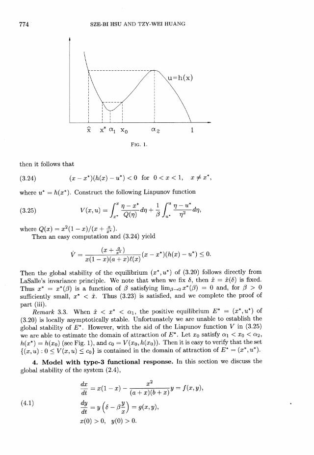
Thus the prey isocline u = h ( x ) has a local maximum and a local minimum at x = na and x = nl, respectively. Obviously h ( 1 ) = 0 , lim,,o+ h ( x ) = +m, and h l ( x ) > 0 for crl < x < a2 and h l ( x ) < 0 for x E (0 , crl) U (a2,1) . Let 2 satisfy 2 > 0 and h ( 2 )= h ( 0 2 ) Then 0 < 2 < 01. (See Fig. I.) Let

SZE-BI HSU AND TZY-WE1 HUANG

then it follows that

(3.24) (x - x*)(h(x)- u*) < 0 for 0 < x < 1, x # x*,

where u* = h(x*). Construct the following Liapunov function

where Q(x) = x2(1- x) / (x + 5 ) . Then an easy computation and (3.24) yield

V = + (x - x*)(h(x)- u*) 5 0. ~ ( lx)(a + x)e(x)-

Then the global stability of the equilibrium (x*, u*) of (3.20) follows directly from LaSalle's invariance principle. We note that when we fix 6, then 2 = 2(6) is fixed. Thus x* = x*(P) is a function of P satisfying limp,o x*(P) = 0 and, for /3 > 0 sufficiently small, x* < 2. Thus (3.23) is satisfied, and we complete the proof of part (iii) .

Remark 3.3. When 2 < x* < c u l , the positive equilibrium E* = (x*,u*) of (3.20) is locally asymptotically stable. Unfortunately we are unable to establish the global stability of E*. However, with the aid of the Liapunov function V in (3.25) we are able to estimate the domain of attraction of E* . Let xo satisfy ail < xo < cu2,

h(x*) = h(xo) (see Fig. I ) , and co = V(xo, h(xo)). Then it is easy to verify that the set {(x, u) : 0 5 V(x, u) < co) is contained in the domain of attraction of E*= (x*, u*).

4. Model with type-3 functional response. In this section we discuss the global stability of the system (2.4),

775 PREDATOR-PREY SYSTEMS

In Remark 2.4, we prove that if (i) a+b > 1 or (ii) a t b < 1 and ( 1 - ( a + b)13 5 27ab, then the positive equilibrium E* = ( x * , y*) is globally asymptotically stable. Hence we restrict our attentions to the following case:

(4.2) a + b < 1 and ( 1 - ( a +b)13 > 27ab.

Under the assumption (4.2) the prey isocline y = h ( x ) = ( l - x ) ( a ~ x ) ( b t x ) has one local minimum and one local maximum in the interval [0,1]and limx,o+ h ( x )= t o o , h ( 1 ) = 0. For the local stability of E* = ( x * , y * ) , it suffices to check (2.7) and (2.8) with h ( x ) = ( l -x)(a~x)ibi . ) . It is easy to verify that (2.8) is satisfied and (2.7) can be rewritten as the following:

where

L E M M A4.1. The equilibrium E* = ( x * , y*) of (4.1) is locally asymptotically stable i f (4.3) holds, and E* is an unstable focus or node i f P ( x * )< 0 .

To find a necessary and sufficient condition for (4.3),we consider P ( x ) and

then P ( x ) > 0 for all 0 5 x < 1. From (4.5), if

and

then P 1 ( x )> 0 for x > 0 , and hence P ( x ) > 0 for all 0 < x 5 1. If D > 0 and (4.7) holds, then from P 1 ( 0 )> 0 and P 1 ( l )> 0 it follows that P 1 ( x )= 0 has two positive roots 0 < cl < c2 < 1, where

and

then P ( x ) > 0 for all 0 < x < 1. If

776 SZE-BI HSU AND TZY-WE1 HUANG

then P ( x ) = 0 has two positive roots al,a 2 satisfying 0 < cl < cul < c2 < a 2 < 1, and P ( x ) can be written as

where a 0 > 0. Under the assumption (4.11), the local asymptotic stability condition (4.3) can be formulated as

We now state and prove our main results in this section. THEOREM4.2. (i) If P ( x ) > 0 for all 0 < x < 1 then the equilibrium E*= (x*, y*) is globally

asymptotically stable in the interior of the first quadrant. (ii) Let (4.11) and (4.14) hold. Then the conclusion of (i) holds.

(iii) Let (4.11) hold. For P > 0 suficiently small, x* = x*(P) is suficiently close to zero and (4.13) holds. Furthermore, the conclusion of (i) holds for P > 0 suficiently small.

(iv) If cul < x* < cu2, then there exists a limit cycle of (4.1). Proof. When cul < x* < cu2, the equilibrium E* is an unstable focus or node.

Thus (iv) follows directly from the Poincark-Bendixon theorem. As in Theorem 3.2 (i) and (ii), it suffices to construct a function H ( x , y) for Dulac's criterion.

Let

where

Then from (4.1) and the hypothesis in (i), an easy computation yields

Hence we complete the proof of (i). For part (ii), the proof is similar to that in part (ii) of Theorem 3.2. Let H ( x , y) =

e(x)r(y), where

for some R > 0 to be chosen, and e(x) satisfies e(x) > 0,

where

PREDATOR-PREY SYSTEMS

Then from (4.15) and (4.16)

where

From (4.17),we have

From (4.17), (4.20), and (4.4),a routine computation yields

( ( ( 1- 6)- 2 x ) ( x 2+ ( a+ b)x + ab) - [-(a + b)x2+ x(-2ab + a + b) + 2abl)

From (4.1) and (4.12) we rewrite I ( x ) in the following form:

( a + x * ) ( b + x * ) ( l- x * ) - ( a + x ) ( b + x ) ( l - x )

(x*12 x2 I

where

To make I ( x ) 5 0 for 0 < x < 1, we shall choose R > 0 satisfying

--

778 SZE-BI HSU AND TZY-WE1 HUANG

Let

and

x2 x + a o x-cul Q ( x ) = x 2 + ~ x + g b + xa + x

Then

x 2 ( x+ a o ) ( x- cul)(4.23) W ( X )= Q ( x )+ (x*-

( a+ x ) ( b+ x ) ( x 2+ A x + $ ) ( x - x * ) '

For x E (0,cul)U ( a z , x * ) , (4.22) holds for any R > 0. From (4.23), the hypothesis x* > cu2, and the fact Q ( x ) is increasing on ( a l ,I ) , it follows that

(4.24) W ( x )< Q ( x )< Q ( a 2 ) for a1 < x < cu2.

Choose R > 0 such that = Q ( a 2 )Then for x* 5 x 5 1, we have

From (4.24) and (4.25), it follows that (4.22) holds. Thus we complete the proof of part (ii) .

As we did in part (iii) of Theorem 3.2, we let u = y l ( x ) , where l ( x )satisfies (3.19)

or l ( x )= (51~;then a routine computation shows that (4.1) can be reduced to the following system:

(4.26) -d u -

- Pu2 ( 2 - x * )d t l ( x ) ( l - x ) ( a + x ) ( b + x ) x *

Consider the prey isocline of (4.26),

From (3.19) and (4 .4) ,an easy computation yields

= { I - a + x + x (x( l-6- ) + x [ ( l- x ) ( a+ x ) ( b+ x)] '(4.28) x 2

779 PREDATOR-PREY SYSTEMS

Thus the prey isocline u = H(x) has a local maximum and local minimum at x = a 2

and x = al, respectively. Obviously, H(1) = 0, limx,o+ H(x) = +m, and H1(x) > 0 for a1 < x < ~ 2 ,and H1(x) < 0 for x E ( 0 , a l )U (a2 , 1). The proof of part (iii) follows directly by constructing a Liapunov function

where

As in Theorem 3.2 (iii), we complete the proof of part (iii).

Remark 4.3. Under the assumption (4.2), the prey isocline h(x) = ( l - x i ( a ~ x ) i b + x )

has precisely one local minimum and one local maximum at xl and x2,O <xl <2 2 <1. We claim that under the assumption (4. l l ) , we have xl < a1 < a 2 < x2, i.e., hl(x) > 0 for all a1 < x 5 a 2 . From (4.27) we have

Differentiating with respect to x yields

Since H(x) has a local minimum and a local maximum at x = a1 and x = a 2 ,

respectively, and l (x) > 0, l l (x) < 0 for 0 < x < 1, from (4.30) it follows that

for i = 1,2. Thus we complete the proof of the claim.

5. Discussion. In this paper we restrict our attention to the analysis of the predator-prey models (1.3),

and

(1.4)

780 SZE-BI HSU AND TZY-WE1 HUANG

These models assume the prey (which is usually referred to as the herbivore [TI) grows logistically with intrinsic growth rate r and carrying capacity K in the absence of predation. The predator consumes the prey according to the functional response p(x) and grows logistically with intrinsic growth rate s and carrying capacity proportional to the population size of the prey. The parameter h in the second equation of (1.3) and (1.4) is the number of herbivores (prey) required to support one predator at equilibrium when the predator density y equals x lh . The intrinsic growth rate s affects not only the potential increase of the predator population, but also its decrease. If y is greater than x lh , the predator population will decline, and the speed of its decline is directly proportional to the instrinsic growth rate s. Species of small body size and early maturity have high intrinsic growth rates. Frequently they also have low survival rates and short lives, and thus their population tends to both grow and decline rapidly [TI. The saturated predator functional response p(x) used in model (1.3) is B,which is of Michaelis-Menten type with half saturation constant A and maximal specific rate m. According to Holling's derivation, A = l /c th and m = 11th where t h equals the handling time per prey item and c is the encounter rate per unit prey density [HO], [HHW2]. The functional response is called Holling's type-2 functional response, and it suits the predators which have only one type of prey to search. The saturated predator functional response p(x) used in model (1.4) is Holling's type-3 functional response The type-3 curve suits the predators which show some form of learning behavior in which, below a certain level of threshold prey density, the predator will not utilize the prey for food at any great intensity. However, above that density level, the predators increase their feeding rates until some saturation level is reached. The sigmoidal functional response is typical for vertebrate predators with alternative prey available.

For the biological interpretations of Theorem 3.2 for model (1.3), there are three important parameters a , 6, and 0.From (2.1), a = A/K is the ratio of half-saturation constant and the carrying capacity of prey, and 6 = is the ratio of intrinsic rate of growth of predator and prey. The parameter can be rewritten as 0= 6 . $. Assuming that the growth of prey is not self-limited at equilibrium, hr is the number of prey to replace the individuals killed by one predator per unit time, while m is the maximal number of prey consumed by a predator per unit time [TI. The results in Theorem 3.2 can be classified into the following cases.

Case I. a 2 1,i.e., K 5 A. From Remark 2.3, if a 2 1then the prey isocline is monotone decreasing and the

equilibrium E* is globally asymptotically stable. Hence, for the small prey carrying capacity, the prey and predator approach constant values, and there is no limiting periodic behavior. We note that in this case the result is independent of the sizes of 6 and 0.

Case 11. a < 1and a + 6 2 1. From Theorem 3.2(i) it follows that the equilibrium E*is globally asymptotically

stable when the prey carrying capacity K is greater than the half-saturation A, and the ratio s / r is larger than 1- a. Then the prey and predator approach equilibrium E*,there is no limiting periodic behavior. In particular, when the intrinsic growth rate s of the predator is greater than the intrinsic growth rate r of the prey, there will be no limit cycle. We note that in this case, the result is independent of the size of 0.

Case 111. a + 6 < 1, (1- a - 612 - 8a6 < 0. It is easy to verify that the necessary and sufficient condition for the above in-

equalities is S1 < 6 < 1- a where S1 = 1+3a -d m > 0.From Theorem 3.2(i),

PREDATOR-PREY SYSTEMS 781

the equilibrium E* is globally asymptotically stable. Hence, when the ratio s / r is not too small, the prey and predator approach equilibrium E*. We note that as in Case 11, the result is independent of the size of /3.

Case IV. a + 6 < 1, (1 - a - 612 - 8a6 > 0. Then 6 satisfies 0< 6 < 61. The numbers ail, a i2 defined in § 3 satisfy 0< ail <

ai2 < 9,and the prey isocline of the system (3.1), y = (1- x)(a + x), attains its maximum at x = 9.There are three subcases.

Subcase (i). a i2 < x* < 1,i.e., (3.7) holds. 602(a+OIZ).The condition is equivalent to (3.7)/, i.e., P > P2 where /I2 = (1-012) Thus,

if 6 is sufficiently small (6 < 61) and is sufficiently large, then the trajectory of (3.1) approaches the equilibrium E* as t + co. Since ai2 < x* < 1 and ai2 < 9 (thus, in particular, if the equilibrium E* is a t the right of the peak of the prey isocline), then E*is globally asymptotically stable. We recall that 6 = :and P = 6 . 2. When the intrinsic growth rate of predator s is sufficiently smaller than that of prey, r and the maximal consumption rate m is sufficiently small, then the prey-predator system (1.3) has no limit cycle.

Subcase (ii). 0< x* < ail, i.e., (3.8) holds. 601The condition is equivalent to (3.8)', i.e., 0< < P1 where P1 = ( l -al)(a+al) .

Thus if 6 and P are both sufficiently small (6 < 61,P < PI),the equilibrium E* is a stable equilibrium. Hence, when the intrinsic growth rate of the predator is sufficiently smaller than that of the prey, and the maximal consumption rate is sufficiently large, the system (1.3) has no limit cycle.

Subcase (iii). ail < x* < 0 2 , i.e., (3.9) holds. The condition is equivalent to (3.9)/, i.e., P1 < /3 < p2. From Theorem 3.2

(iv), there exists a limit cycle for the predator-prey system. Thus it is a necessary condition for the existence of the limit cycle that :be sufficiently small. The condition /3l < P < P2 means that the maximal consumption rate cannot be too small or too large for the existence of the limit cycle.

The biological interpretations of Theorem 4.2 for model (1.4) with type-3 func- tional response are similar to those of model (1.3) with type-2 functional response. We note that the constants A and B in the type-3 functional response are obtained from the S-shaped curve by "curve fitting." The results in Theorem 4.2 can be classified into the following cases.

Case I. (i)a + b > 1or (ii) a + b < 1 and (1 - (a + b)13 5 27ab. The prey isocline of (4.1) is monotone decreasing, and the global asymptotic

stability of E* follows directly from Remark 2.4. From (2.1), we have a = $ and b = a. Hence, for small prey carrying capacity K, the prey and predator approach constant values. The result in this case is independent of the sizes of 6 and P.

Case 11. a + b < 1and (1 - (a + b)13 > 27ab, 6 > 1- (a + b). From Theorem 4.2 (i) it follows that the equilibrium E*is globally asymptotically

stable. Under the conditions a + b < 1 and (1 - (a + b)13 > 27ab, i.e., the carrying capacity K of prey is sufficiently large, if the ratio s / r is larger than 1- (a + b), then the prey and predator approach equilibrium E*. In particular, when the intrinsic growth rate s of the predator is greater than the intrinsic growth rate r of the prey, there will be no limit cycle. We note that in this case, the result is independent of the size of p.

Case 111. a + b < 1, (1 - (a + b)13 > 27ab; 0< 6 < 1- (a+b); (1 - (a + b) - 612-6(a + b)6 5 0.

782 SZE-BI HSU AND TZY-WE1 HUANG

As in Case I11 for model (1.3), the above conditions mean 0 < 61 < 6 < 1- (a+b), where S1 = 2(a+ b) +1- J3(a + b) ((a + b) + 2). From Theorem 4.2(i), the equilibrium E* is globally asymptotically stable. Hence when the ratio s / r is not too small, the prey and predator approach equilibrium E* . The result is independent of the size of p.

Case IV. a+b < 1, (1 - ( a + b)13 > 27ab; 0 < 6 < 1-(a+b); (1- ( a + b) - 6)'-6(a + b)6 > 0; P(cz) 2 0.

The condition (4.10), P(cz) > 0, means the ratio 6 is bounded away from zero. It is easy to verify that when 6 = 0, we have cz = and P(cz) = ab -&(1 - (a + b)13 < 0. The biological interpretation for this case is the same as in Case I11 above.

Case V. a + b < 1, (1- (a + b)13 > 27ab; 0 < 6 < 1- ( a + b); (1 - (a + b) - 6)' -6(a + b)6 > 0; P(c2) < 0.

From the analysis in §4, the condition for asymptotic stability of E* is either (4.13) or (4.14). The condition a1 < x* < a 2 is the instability condition for E*. From Remark 4.3, we have ht(ai) > 0, i = 1,2, where h(x) = ( l - x ) ( a ~ x ) ( b + x ) is the prey isocline of (4.1). Thus, in particular, if the equilibrium E* is at the right of the peak of the prey isocline or at the left of the bottom of the prey isocline, then E* is a stable equilibrium. The biological interpretations basically are the same as those of Case IV for the type-2 case. We omit them.

In §§ 3 and 4 we gave a global analysis of the asymptotic behavior of the well- known Holling-Tanner model (3.1) and the model (4.1) with a type-3 functional re- sponse. The mathematical results are by no means complete. In fact, we are unable to prove the global stability of the positive equilibrium E*for the case (3.8), (4.13) in the model (3.1) and (4.1), respectively. However, with a change of variable in (3.17) we reduce (3.1), (4.1) to a Gause-type predator-prey system (3.20), (4.26), respectively. By constructing a Liapunov function, we show that for P > 0 sufficiently small, E* is globally asymptotically stable.

There are two interesting problems that remain open. One is to prove the global stability of E*for the case (3.8) and (4.13) for the model (3.1) and (4.1), respectively. The other is the problem of the uniqueness of the limit cycle for the case a1 < x* < a2. We conjecture that the reduced system (3.20), (4.26) should play an important role in dealing with these problems.

Acknowledgments. The first author would like to thank Professor Yang Kuang of Arizona State University for introducing him to the global stability problem of the Holling-Tanner model.

REFERENCES

[BHW] G. J . BUTLER,S. B. HSU, AND P. WALTMAN,Coexis tence of compet ing predators in a chemos ta t , J . Math. Biology, 17(1983), pp. 133-151.

[CHL] K. S. CHENG, S. B. HSU, AND S. S. LIN, S o m e resul ts o n global stability of a predator-prey s y s t e m , J . Math. Biology 12(1981), pp. 115-126.

[FM] H. I. FREEDMAN Persis tence in predator-prey s y s t e m s w i t h ratio- AND R. M. MATHSEN, dependence predat ion in f luence, Bull. Math. Biol., 55(1993), pp. 817-827.

[GI B. S. GOH, Global stability in m a n y species s y s t ems , Emer. Natur. 111(1977), pp. 135-143.

[HI J. K . HALE,Ordinary Differential Equat ions , Wiley-Interscience, New York, 1969. [HHWl] S. B. Hsu, S. P. HUBBELL, P. WALTMAN,AND Compe t ing predators, SIAM J. Appl.

Math., 35(1978), pp. 525-617. [HHWP] -, A contr ibut ion t o t h e theory of compet ing species, Ecological Monographs,

48(1978), pp. 337-349.

783 P R E D A T O R - P R E Y S Y S T E M S

S . B . H S U , O n global stability of apredator-prey sys t em, M a t h . Biosci. , 39(1978), pp. 1-10. C . S . HOLLING, T h e funct ional response of predators t o prey dens i t y and i t s role in

m i m i c r y and population regulation, M e m . E n t . Soc . Can . , 46(1965), pp. 1-60. Y . K U A N G , Global stability of Gause- type predator-prey sys t ems , J . M a t h . Biology,

28(1990), pp. 463-474 T . L I N D S T R O M ,Qualitative analyszs of a predator-prey s y s t e m wi th l imi t cycles, J . M a t h .

Biol . , 31(1993), pp. 541-561. L . P . LIOU A N D K . S . C H E N G , Global stability of a predator-prey sys t em, J . M a t h . Biol.,

26(1988), pp. 26-71. P . H . L E S L I E A N D J . C . GOWER, T h e properties of a stochastic model for the predator-prey

type of in teract ion between t w o species, Biometr ika, 47(1960), pp. 219-234. J . D . MURRAY, Mathematical Biology, Springer-Verlag, Berl in , 1989. R . M . MAY, Stability and Complexi ty in Model Ecosystems, Princeton Univers i t y Press,

Princeton, N J , 1974. E . RENSHAW,Modelling Biological Populat ions in Space and T i m e , Cambr idge Univers i t y

Press, Cambr idge , U . K . , 1991. L . A . REAL,T h e kinet ics of functional response, Amer ican Natural is t , 111(1977), pp. 289-

300. J . MAYNARD S M I T H , Models in Ecology, Cambr idge Univers i ty Press, Cambr idge , U .K . ,

1974. J . T . TANNER,T h e stability and t h e intr ins ic growth rates of prey and predator popula-

t i ons , Ecology, 56(1975), pp. 855-867.