Embed Size (px)
Citation preview
HSUPA Performance in Indoor Environments
Pedro Miguel Cardoso Ferreira
Dissertation to obtain the Master degree in
Electrotechnical and Computers Engineering
Jury
Supervisor: Prof. António Rodrigues
President: Prof. Bioucas Dias
Member: Prof. Francisco Cercas
November 2009

i
Agradecimentos
Em primeiro lugar quero agradecer ao Professor António Rodrigues ter aceitado orientar a
proposta de dissertação por mim apresentada. Bem como todo o seu apoio e valiosas
indicações e sugestões durante todo o processo que conduziu a este documento.
Quero também agradecer a todos os meus colegas de trabalho na TMN que contribuíram de
algum modo para a realização desta dissertação. Em especial ao João Figueiredo e ao João
Romão por toda a ajuda prestada que facilitou em muito a realização deste trabalho.
Quero agradecer à Beatriz pelo seu constante apoio, companhia e carinho. Pela quase
infindável paciência nos momentos mais críticos. E ainda pelas dicas e revisão dos vários
textos.
Quero agradecer aos meus pais que me ensinaram a ser persistente e sempre me
incentivaram a ir mais além, e a escolher livremente o meu caminho. Bem como ao meu irmão
que partilha comigo muitos dos meus melhores e piores momentos, sendo sempre capaz de
me chamar à realidade e animar nas alturas certas.
Finalmente queria agradecer aos meus amigos e familiares, que me fizeram sentir sempre
acompanhado, apesar do menor tempo que dispus para eles.

ii
iii
Abstract
The present dissertation intends to study the performance of High Speed Uplink Packet Access
(HSUPA) in a commercial network, in indoor scenarios with different coverage solutions. The
tests were conducted in indoor locations with four different coverage solutions, namely: indoor
coverage provided by outdoor sites, indoor dedicated site, optical repeater and Radio
Frequency (RF) repeater.
For each test scenario three locations with different characteristics were tested, by performing
extensive FTP uploads. These tests were performed using a power class 3 HSUPA compatible
category 3 UE. With this test setup a maximum throughput of 1,45 Mbps can be expected at the
air interface. From the tests a group of metrics were collected in order to evaluate the
performance and network impact of the tested service. Among these metrics were the received
signal strength, receive signal quality, UE transmission power, received total wideband noise
and data throughput.
Based on the collected results one can confirm the major upgrade brought by HSUPA to the
uplink data transfers in UMTS, with average application throughputs close to 1,2 Mbps. The
impact on the cell noise rise was in general small, though there is a clear difference between
the scenarios with and without repeaters, especially the optical repeater scenario. The achieved
results were good, nevertheless one has to mention that the tests were performed under good
radio conditions and the UE almost never reach is maximum power. In more challenging radio
environments and/or with higher category UE the achieved results might be different.
Keywords HSUPA, indoor, real live performance, throughput.

iv
v
Resumo
A dissertação aqui apresentada propõe-se estudar a performance do HSUPA numa rede
comercial, recorrendo a testes em cenários indoor com diferentes soluções de cobertura. Os
testes foram efectuados em quarto diferentes cenários: cobertura indoor através de sites
outdoor, site indoor dedicado, repetidor óptico e repetidor RF.
Para cada cenário de testes, os mesmos foram realizados em três locais com diferentes
características efectuando-se, em cada um deles, um grande conjunto de uploads via FTP.
Estes testes foram efectuados utilizando um equipamento terminal compatível com HSUPA de
classe de potência 3 e pertencente à categoria 3. Com este tipo de equipamento poderemos
esperar uma velocidade máxima de transferência na interface ar de 1,45 Mbps. Dos testes
realizados foram recolhidos um grupo de medidas de forma a avaliar a performance do serviço
e o seu impacto na rede. Nestas medidas incluem-se o Ec, Ec/I0, UETxPwr, RTWP e
velocidade de transferência.
Com base nos resultados obtidos confirma-se que o HSUPA constitui uma enorme melhoria na
capacidade de transferência de dados em uplink do UMTS, chegando a velocidades de
transferência ao nível da aplicação perto dos 1,2 Mbps. Por outro lado, o impacto no nível de
interferência no receptor é em geral pequeno, embora exista uma clara diferença entre os
cenários com e sem repetidor, em especial no caso do repetidor óptico. Os resultados obtidos
podem considerar-se bons, no entanto dever-se-á ter em conta que os testes actuais foram
realizados sobre boas condições rádio e onde o equipamento móvel raramente atingiu a sua
potência máxima. Num ambiente com piores condições rádio e/ou com um equipamento
terminal de categoria superior os resultados obtidos poderão ser diferentes destes.
Palavras-chave HSUPA, indoor, performance em rede real, velocidade de transferência.

vi
vii
Table of contents
Agradecimentos.............................................................................................................................. i
Abstract ......................................................................................................................................... iii
Resumo ......................................................................................................................................... v
Table of contents .......................................................................................................................... vii
List of Figures ................................................................................................................................ ix
List of Tables ................................................................................................................................. xi
List of Acronyms .......................................................................................................................... xiii
List of Symbols ............................................................................................................................. xv
1 Introduction ........................................................................................................................... 1
1.1 Overview ...................................................................................................................... 2
1.2 Motivation and contents ............................................................................................... 3
2 HSUPA Basics ...................................................................................................................... 5
2.1 UMTS Basic Description .............................................................................................. 6
2.1.1 UMTS Architecture .................................................................................................. 6
2.1.2 Radio Interface ........................................................................................................ 8
2.1.3 HSDPA .................................................................................................................. 10
2.2 HSUPA Description .................................................................................................... 12
2.2.1 HSUPA Features and Channels ............................................................................ 12
2.2.2 HSUPA Performance ............................................................................................. 14
2.3 Beyond HSUPA.......................................................................................................... 17
2.3.1 HSPA improvements ............................................................................................. 17
2.3.2 LTE basics ............................................................................................................. 20
3 Test Scenarios .................................................................................................................... 23
3.1 Introduction ................................................................................................................ 24
3.2 Test methodology....................................................................................................... 24
3.3 Coverage and capacity .............................................................................................. 25
3.4 Indoor coverage by outdoor sites............................................................................... 28
3.4.1 Test description ..................................................................................................... 28
3.4.2 Link and capacity budget ....................................................................................... 29
3.5 Dedicated indoor site ................................................................................................. 32
3.5.1 Test description ..................................................................................................... 32
3.5.2 Link and capacity budget ....................................................................................... 33
3.6 Repeater indoor site ................................................................................................... 34
3.6.1 Optical Repeater .................................................................................................... 35
3.6.2 RF Repeater .......................................................................................................... 37
4 Test Results ........................................................................................................................ 41
viii
4.1 Introduction ................................................................................................................ 42
4.2 Outdoor Site ............................................................................................................... 42
4.3 Dedicated Site ............................................................................................................ 48
4.4 Optical Repeater ........................................................................................................ 53
4.5 RF Repeater ............................................................................................................... 58
4.6 Global results ............................................................................................................. 63
5 Conclusions and Future Work ............................................................................................ 67
5.1 Conclusions ................................................................................................................ 68
5.2 Future Work ............................................................................................................... 69
Annex I - Propagation Models ..................................................................................................... 71
Annex II - Additional Test Results ............................................................................................... 77
References .................................................................................................................................. 85
ix
List of Figures Figure 1.1: Technology standards for wireless broadband access [1] .......................................... 3
Figure 2.1: UMTS architecture [9] ................................................................................................. 7
Figure 2.2: UMTS spectrum allocation [10] ................................................................................... 8
Figure 2.3: UMTS R99 transport and physical channels [11] ..................................................... 10
Figure 2.4: Active HSDPA Channels [12] .................................................................................... 11
Figure 2.5: HSUPA channels [12] ............................................................................................... 12
Figure 2.6: HSUPA UE categories [12] ....................................................................................... 14
Figure 2.7: Noise rise distribution [12] ......................................................................................... 15
Figure 2.8: Vehicular A – 30 km/h Single User throughput [12] .................................................. 16
Figure 2.9: Noise rise due to a single user [12] ........................................................................... 17
Figure 2.10: 2x2 MIMO System [14]............................................................................................ 18
Figure 2.11: WCDMA UE States [14] .......................................................................................... 19
Figure 2.12: OFDM subcarrier scheme [14] ................................................................................ 20
Figure 2.13: OFDM subcarrier symbol [14] ................................................................................. 21
Figure 2.14: LTE architecture [14] ............................................................................................... 21
Figure 3.1: Test Setup ................................................................................................................. 24
Figure 3.2: Indoor covered by outdoor site layout ....................................................................... 29
Figure 3.3: Indoor dedicated site layout ...................................................................................... 32
Figure 3.4: Indoor dedicated site block diagram ......................................................................... 33
Figure 3.5: Optical repeater site layout ....................................................................................... 35
Figure 3.6: Optical repeater site block diagram .......................................................................... 36
Figure 3.7:RF repeater site layout ............................................................................................... 37
Figure 3.8: RF repeater site block diagram ................................................................................. 38
Figure 4.1: P1-Window Throughput vs Ec, Ec/I0 .......................................................................... 43
Figure 4.2: P2-Indoor Throughput vs Ec, Ec/I0 ............................................................................. 44
Figure 4.3: P3-Deep Indoor Throughput vs Ec, Ec/I0 ................................................................... 45
Figure 4.4: Throughput [kbps], Ec, Ec/I0 for outdoor site scenario ............................................... 46
Figure 4.5: Radio conditions for outdoor site scenario ................................................................ 47
Figure 4.6: UE Tx power for outdoor site scenario...................................................................... 47
Figure 4.7: Data session statistics in outdoor site scenario ........................................................ 47
Figure 4.8: RTWP in outdoor site scenario ................................................................................. 48
Figure 4.9: P1-Window Throughput vs Ec, Ec/I0 .......................................................................... 49
Figure 4.10: P2-Antenna Throughput vs Ec, Ec/I0........................................................................ 50
Figure 4.11: P3-Indoor Throughput vs Ec, Ec/I0 ........................................................................... 51
Figure 4.12: Throughput [kbps], Ec, Ec/I0 for dedicated site scenario ......................................... 51
Figure 4.13: Radio conditions for dedicated site scenario .......................................................... 52
Figure 4.14: UE Tx power for dedicated site scenario ................................................................ 52
x
Figure 4.15: Data session statistics in dedicated site scenario ................................................... 53
Figure 4.16: RTWP in dedicated site scenario ............................................................................ 53
Figure 4.17: P1-Window Throughput vs Ec, Ec/I0 ........................................................................ 54
Figure 4.18: P2-Antenna Throughput vs Ec, Ec/I0........................................................................ 55
Figure 4.19: P3-Indoor Throughput vs Ec, Ec/I0 ........................................................................... 56
Figure 4.20: Throughput [kbps], Ec, Ec/I0 for optical repeater scenario ....................................... 56
Figure 4.21: Radio conditions for optical repeater scenario ........................................................ 57
Figure 4.22: UE Tx power for optical repeater scenario ............................................................. 57
Figure 4.23: Data session statistics in optical repeater scenario ................................................ 57
Figure 4.24: RTWP in optical repeater scenario ......................................................................... 58
Figure 4.25: P1-Window Throughput vs Ec, Ec/I0 ........................................................................ 59
Figure 4.26: P2-Antenna Throughput vs Ec, Ec/I0........................................................................ 60
Figure 4.27: P3-Indoor Throughput vs Ec, Ec/I0 ........................................................................... 61
Figure 4.28: Throughput [kbps], Ec, Ec/I0 for optical repeater scenario ....................................... 61
Figure 4.29: Radio conditions for RF repeater scenario ............................................................. 62
Figure 4.30: UE Tx power for RF repeater scenario ................................................................... 62
Figure 4.31: Data session statistics in RF repeater scenario ...................................................... 62
Figure 4.32: RTWP in RF repeater scenario ............................................................................... 63
Figure 4.33: Ec and Ec/I0 in all test scenarios .............................................................................. 63
Figure 4.34: UE Tx Power in all test scenarios ........................................................................... 64
Figure 4.35: Rise over thermal all test scenarios ........................................................................ 64
Figure 4.36: Throughput in all test scenarios .............................................................................. 65
Figure A2.0.1: Outdoor site P1 throughput relation with ............................................................. 79
Figure A2.0.2: Outdoor site P2 throughput relation with ............................................................. 79
Figure A2.0.3: Outdoor site P3 throughput relation with ............................................................. 80
Figure A2.0.4: Dedicated site P1 throughput relation with .......................................................... 80
Figure A2.0.5: Dedicated site P2 throughput relation with .......................................................... 80
Figure A2.0.6: Dedicated site P3 throughput relation with .......................................................... 81
Figure A2.0.7: Optical repeater P1 throughput relation with ....................................................... 81
Figure A2.0.8: Optical repeater P2 throughput relation with ....................................................... 81
Figure A2.0.9: Optical repeater P3 throughput relation with ....................................................... 82
Figure A2.0.10: RF repeater P1 throughput relation with ........................................................... 82
Figure A2.0.11: RF repeater P2 throughput relation with ........................................................... 82
Figure A2.0.12: RF repeater P3 throughput relation with ........................................................... 83
xi
List of Tables
Table 2.1: UMTS traffic classes summary [8] ............................................................................... 6
Table 2.2: DPDCH and E-DPDCH comparison [12] ................................................................... 13
Table 2.3: Simulation Assumptions [12] ...................................................................................... 16
Table 3.1: Generic HSUPA link budget ....................................................................................... 25
Table 3.2: Indoor UE to outdoor BTS link budget ....................................................................... 30
Table 3.3: Indoor dedicated site link budget ............................................................................... 34
Table 3.4: Optical repeater site link budget ................................................................................. 36
Table 3.5: RF repeater site link budget ....................................................................................... 39
Table 4.1: P1-Window Statistics.................................................................................................. 42
Table 4.2: P2-Indoor Statistics .................................................................................................... 43
Table 4.3: P3-Deep Indoor Statistics........................................................................................... 45
Table 4.4: P1-Window Statistics.................................................................................................. 49
Table 4.5: P2-Antenna Statistics ................................................................................................. 50
Table 4.6: P3-Indoor Statistics .................................................................................................... 50
Table 4.7: P1-Window Statistics.................................................................................................. 54
Table 4.8: P2-Antenna Statistics ................................................................................................. 55
Table 4.9: P3-Indoor Statistics .................................................................................................... 55
Table 4.10: P1-Window Statistics ................................................................................................ 59
Table 4.11: P2-Antenna Statistics ............................................................................................... 59
Table 4.12: P3-Indoor Statistics .................................................................................................. 60

xii
xiii
List of Acronyms 16QAM 16 Quadrature Amplitude Modulation
2G Second Generation
3G Third Generation
3GPP Third Generation Partnership Project
ACK Acknowledgement
BLER Block Error Rate
BTS Base Transceiver Station
CN Core Network
CPC Continuous Packet Connectivity
CQI Channel Quality Information
CRC Cyclic Redundancy Check
CS Circuit Switch
DAS Distributed Antenna System
DCH Dedicated Channel
DL Downlink
DPDCH Dedicated Physical Data Channel
DRX Discontinuous Reception
DTX Discontinuous Transmission
E-AGCH E-DCH Absolute Grant Channel
E-DCH Enhanced Dedicated Channel
E-DPDCH Enhanced Dedicated Physical Data Channel
E-DPCCH Enhanced Dedicated Physical Control Channel
E-HICH E-DCH HARQ Indicator Channel
E-RGCH E-DCH Relative Grant Channel
E-TFCI E-DCH Transport Format Indicator
EIRP Equivalent Isotropic Radiated Power
FACH Forward Access Channel
FDD Frequency Division Duplex
FTP File Transfer Protocol
GGSN Gateway GPRS Support Node
GPRS General Packet Radio System
GSM Global System for Mobile Communications
HARQ Hybrid Automatic Repeat Request
HBW Horizontal Beam Width
HS-DPCCH High Speed Dedicated Physical Control Channel
HS-DSCH High Speed Downlink Shared Channel
HS-SCCH High Speed Shared Control Channel
xiv
HSDPA High Speed Downlink Packet Access
HSPA High Speed Packet Access
HSUPA High Speed Uplink Packet Access
IP Internet Protocol
L1 Layer One
LOS Line Of Sight
LTE Long Term Evolution
MBMS Multimedia Broadcast Multicast Service
ME Mobile Equipment
MIMO Multiple Input Multiple Output
MSC Mobile Switching Centre
NACK Negative Acknowledgement
NLOS Non Line Of Sight
NR Noise Rise
OFDM Orthogonal Frequency Division Multiplexing
PS Packet Switch
QoS Quality of Service
QPSK Quaternary Phase Shift Keying
RAB Radio Access Bearer
RSCP Received Signal Code Power
RTWP Received Total Wideband Power
RF Radio Frequency
RNC Radio Network Controller
RNS Radio Network Subsystem
SC Scrambling Code
SF Spreading Factor
SGSN Serving GPRS Support Node
SIR Signal to Interference Ratio
SPI Scheduling Priority Indicator
TBS Transport Block Size
TDD Time Division Duplex
TMA Tower Mounted Amplifier
TTI Time Transmission Interval
UE User Equipment
UL Uplink
UMTS Universal Mobile Terrestrial System
USIM UMTS Subscriber Identity Module
UTRAN UMTS Terrestrial Radio Access Network
VoIP Voice over IP
WCDMA Wideband Code Division Multiple Access
xv
List of Symbols
f∆ Frequency separation for OFDM carriers
ULη Uplink load factor
jυ User j activity factor
ψ Street incidence angle
b Empirical correction parameter for penetrated floors
bE Energy per bit
cE Energy per chip
f Frequency
TMAG TMA gain
BH BTS antenna height
Bh Mean building height
mh Mobile height
i Other to own cell interference ratio
0I Interference density
aK Loss due to adjacent buildings
dK Dependence of multi screen diffraction with distance
fK Dependence of multi screen diffraction with frequency
wik Number of type i penetrated walls
0L Free space loss
bshL Loss due to BTS antenna height
cL Correction to measured wall losses
cableL Antenna to BTS cable loss
fL Loss between adjacent floors
oriL Loss due to street incidence angle
pL Path Loss
ttL Multi screen diffraction loss
tmL Rooftop to UE diffraction and scatter losses
wiL Loss of type i walls
n Number of penetrated floors
N Number of users
0N Noise spectral density
BTSNF BTS noise figure

xvi
TMANF TMA noise figure
poleN Pole capacity
R Cell radius
jR User j bit rate
GainTMA Improvement due to TMA
uT OFDM pulse duration
W WCDMA chip rate
bw Building separation
Sw Street width

1
1 Introduction
This chapter presents a brief introduction on the evolution of mobile wireless networks to this
day and future trends. Further some references on previous work on HSUPA and indoor
coverage is given. Finally the structure of the current document is presented.
2
1.1 Overview
The advent of mobile communication systems, specially the huge success of second generation
(2G) systems from which Global System for Mobile Communications (GSM) is by far the most
popular worldwide, changed the way people communicate and ultimately their way of life.
Nowadays people are permanently reachable on their mobile phones, improving their efficiency
at work or allowing to keeping easily in touch with their friends and family.
The main goal for the third generation (3G) system was to provide this ubiquitous
communication experience not only for voice but to a large set of data based services, making
internet access available anytime and anywhere through a simple and fast setup process. To
achieve this goal the Third Generation Partnership Project (3GPP) established in 1999 the
standards for a global third generation mobile system: UMTS – Universal Mobile Terrestrial
System, based in WCDMA - Wideband Code Division Multiple Access. This so called R99
release enabled data transfer with peak rates of 384 kbps and allowed full mobility.
Although R99 was a major step forward towards global wireless packet access, some
improvements were yet to be made. During the work made on future releases of the standard it
became clear that the packet access performance of the system should be improved in order to
cope with the available and future services and to compete with a variety of other wireless
packet access technologies. In order to improve the data rates in the downlink a new feature:
High Speed Downlink Packet Access (HSDPA) was defined by 3GPP in 2002 R5 release. R5
HSDPA theoretical downlink maximum peak rate is 14,4 Mbps, however with new releases
developments should in the near future reach 21 Mbps.
Following the definition of a new standard to improve downlink performance and capacity, the
focus of 3GPP moved to the specification of a new feature that would improve the uplink
performance. From that effort was finally released in 2005 the R6 which presented the new
Frequency Division Duplex (FDD) Enhanced Uplink feature, commonly known as HSUPA –
High Speed Uplink Packet Access. This new feature will allow a maximum peak rate of 5,76
Mbps; current implementations permit rates up to 2 Mbps.
Though not widely implemented in commercial products, 3GPP already finished the standard for
release R7 and is working now in release R8. These releases present important enhancements
to HSDPA and HSUPA, now commonly known as High Speed Packet Access - HSPA. With
these improvements the maximum theoretical rates at the air interface will be increased to 42
Mbps in the downlink and 11,5 Mbps in the uplink.
3
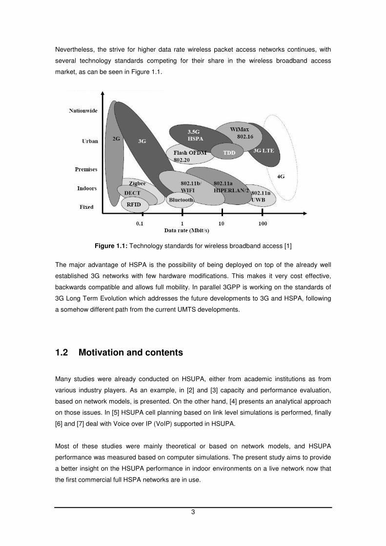
Nevertheless, the strive for higher data rate wireless packet access networks continues, with
several technology standards competing for their share in the wireless broadband access
market, as can be seen in Figure 1.1.
Figure 1.1: Technology standards for wireless broadband access [1]
The major advantage of HSPA is the possibility of being deployed on top of the already well
established 3G networks with few hardware modifications. This makes it very cost effective,
backwards compatible and allows full mobility. In parallel 3GPP is working on the standards of
3G Long Term Evolution which addresses the future developments to 3G and HSPA, following
a somehow different path from the current UMTS developments.
1.2 Motivation and contents
Many studies were already conducted on HSUPA, either from academic institutions as from
various industry players. As an example, in [2] and [3] capacity and performance evaluation,
based on network models, is presented. On the other hand, [4] presents an analytical approach
on those issues. In [5] HSUPA cell planning based on link level simulations is performed, finally
[6] and [7] deal with Voice over IP (VoIP) supported in HSUPA.
Most of these studies were mainly theoretical or based on network models, and HSUPA
performance was measured based on computer simulations. The present study aims to provide
a better insight on the HSUPA performance in indoor environments on a live network now that
the first commercial full HSPA networks are in use.
4
This document comprises five chapters, including this Introduction and a final Conclusion.
Chapter 2 presents a basic description of UMTS with a special focus on HSUPA, based on what
was defined by 3GPP in release R6. It also presents some of ongoing and future HSUPA
enhancements and a brief description of Long Term Evolution - LTE. Chapter 3 presents a
complete description of the test methodology as well as a full description of the test scenarios
and test details for each scenario. The tests were conducted in four different scenarios: indoor
coverage by outdoor sites, dedicated indoor site with distributed antenna system, dedicated
indoor coverage with fibre optics repeater and dedicated indoor coverage with RF repeater. For
each of the test scenarios a theoretical approach on the expected results is also presented.
Finally, Chapter 4 presents the results of the tests for the various scenarios and collected
metrics.
5
2 HSUPA Basics
This chapter presents a basic description of some of the most important aspects of HSUPA. In
2.1 a more general presentation of the UMTS system is given, whilst 2.2 contains a more
detailed description of HSUPA. Finally, in 2.3 is presented the current work on HSUPA
performance enhancement as well as the path towards LTE.
6
2.1 UMTS Basic Description
In the late nineties it became clear that the hugely popular 2G systems were not suited for data
packet transfers. This led to the creation of 3GPP which took the responsibility of creating a new
standard to allow a fully mobile wireless broadband access either for voice and circuit switch
calls as well for packet switch data sessions. The outcome of this work came in 1999, with a
brand new set of specifications that established UMTS.
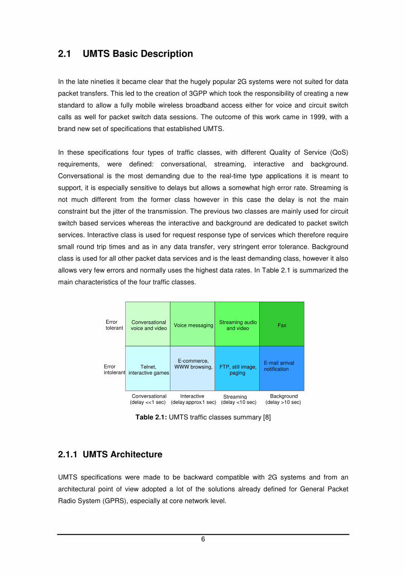
In these specifications four types of traffic classes, with different Quality of Service (QoS)
requirements, were defined: conversational, streaming, interactive and background.
Conversational is the most demanding due to the real-time type applications it is meant to
support, it is especially sensitive to delays but allows a somewhat high error rate. Streaming is
not much different from the former class however in this case the delay is not the main
constraint but the jitter of the transmission. The previous two classes are mainly used for circuit
switch based services whereas the interactive and background are dedicated to packet switch
services. Interactive class is used for request response type of services which therefore require
small round trip times and as in any data transfer, very stringent error tolerance. Background
class is used for all other packet data services and is the least demanding class, however it also
allows very few errors and normally uses the highest data rates. In Table 2.1 is summarized the
main characteristics of the four traffic classes.
Errortolerant
Errorintolerant
Conversational(delay <<1 sec)
Interactive(delay approx.1 sec)
Streaming(delay <10 sec)
Background(delay >10 sec)
Conversationalvoice and video
Voice messagingStreaming audio
and videoFax
E-mail arrivalnotificationFTP, still image,
paging
E-commerce,WWW browsing,Telnet,
interactive games
Table 2.1: UMTS traffic classes summary [8]
2.1.1 UMTS Architecture
UMTS specifications were made to be backward compatible with 2G systems and from an
architectural point of view adopted a lot of the solutions already defined for General Packet
Radio System (GPRS), especially at core network level.
7
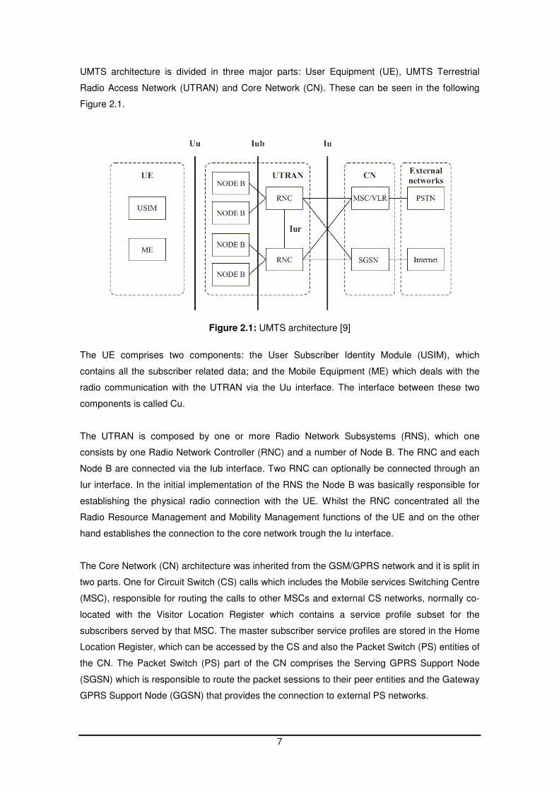
UMTS architecture is divided in three major parts: User Equipment (UE), UMTS Terrestrial
Radio Access Network (UTRAN) and Core Network (CN). These can be seen in the following
Figure 2.1.
Figure 2.1: UMTS architecture [9]
The UE comprises two components: the User Subscriber Identity Module (USIM), which
contains all the subscriber related data; and the Mobile Equipment (ME) which deals with the
radio communication with the UTRAN via the Uu interface. The interface between these two
components is called Cu.
The UTRAN is composed by one or more Radio Network Subsystems (RNS), which one
consists by one Radio Network Controller (RNC) and a number of Node B. The RNC and each
Node B are connected via the Iub interface. Two RNC can optionally be connected through an
Iur interface. In the initial implementation of the RNS the Node B was basically responsible for
establishing the physical radio connection with the UE. Whilst the RNC concentrated all the
Radio Resource Management and Mobility Management functions of the UE and on the other
hand establishes the connection to the core network trough the Iu interface.
The Core Network (CN) architecture was inherited from the GSM/GPRS network and it is split in
two parts. One for Circuit Switch (CS) calls which includes the Mobile services Switching Centre
(MSC), responsible for routing the calls to other MSCs and external CS networks, normally co-
located with the Visitor Location Register which contains a service profile subset for the
subscribers served by that MSC. The master subscriber service profiles are stored in the Home
Location Register, which can be accessed by the CS and also the Packet Switch (PS) entities of
the CN. The Packet Switch (PS) part of the CN comprises the Serving GPRS Support Node
(SGSN) which is responsible to route the packet sessions to their peer entities and the Gateway
GPRS Support Node (GGSN) that provides the connection to external PS networks.
8
2.1.2 Radio Interface
The technology used in the UMTS radio interface is the Wideband Code Division Multiple
Access (WCDMA). During standardization was defined a 5MHz bandwidth for each UMTS
carrier and two different modes: Frequency Division Duplex (FDD) and Time Division Duplex
(TDD). Currently there are already plenty of UMTS FDD networks deployed around the world.
FDD mode uses two sub-bands one for downlink another for uplink allowing a full duplex
communication, whilst TDD mode does the same by time multiplexing of downlink and uplink.
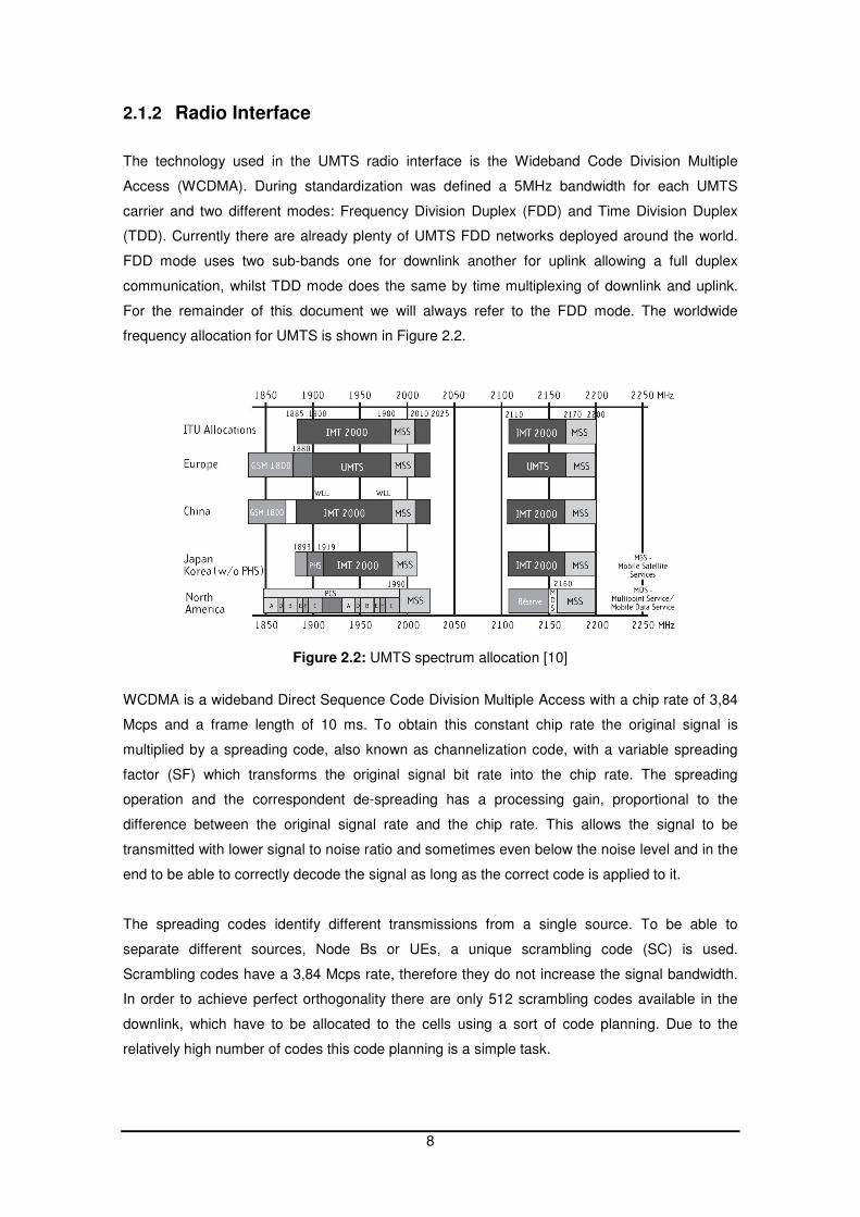
For the remainder of this document we will always refer to the FDD mode. The worldwide
frequency allocation for UMTS is shown in Figure 2.2.
Figure 2.2: UMTS spectrum allocation [10]
WCDMA is a wideband Direct Sequence Code Division Multiple Access with a chip rate of 3,84
Mcps and a frame length of 10 ms. To obtain this constant chip rate the original signal is
multiplied by a spreading code, also known as channelization code, with a variable spreading
factor (SF) which transforms the original signal bit rate into the chip rate. The spreading
operation and the correspondent de-spreading has a processing gain, proportional to the
difference between the original signal rate and the chip rate. This allows the signal to be
transmitted with lower signal to noise ratio and sometimes even below the noise level and in the
end to be able to correctly decode the signal as long as the correct code is applied to it.
The spreading codes identify different transmissions from a single source. To be able to
separate different sources, Node Bs or UEs, a unique scrambling code (SC) is used.
Scrambling codes have a 3,84 Mcps rate, therefore they do not increase the signal bandwidth.
In order to achieve perfect orthogonality there are only 512 scrambling codes available in the
downlink, which have to be allocated to the cells using a sort of code planning. Due to the
relatively high number of codes this code planning is a simple task.
9
One of the benefits of such a wideband signal is to take a bigger advantage of the typical
multipath propagation of a radio channel. Multipath components with smaller time difference can
be individually distinguished and therefore coherently combined in order to obtain multipath
diversity. This is done with the help of a Rake receiver which comprises several fingers tuned to
the strongest multipath components that are afterwards processed with gain relative to the main
path, which provides multipath diversity against fading.
WCDMA uses a very tight frequency reuse pattern, normally a 1:1 reuse pattern, making it an
interference limited system. Therefore power control is amongst the most important features in
UMTS, the absence of power control would cause a single UE to possibly block an entire cell, or
a Node B to increase the interference in other cells seriously affecting their capacity. There are
two kinds of power control mechanisms: close loop power control and outer loop power control.
Outer loop power control is set at RNC level and takes into account the Radio Access Bearer
(RAB) requirements in terms of Eb/N0 and Block Error Rate (BLER) target, it also follows the
long term radio environment variations. Closed loop power control on the other hand is a fast
power control mechanism with a frequency of 1500 times per second, which tries to
compensate for fast fading variations of the radio channel, aiming to follow in small up and
down steps, the Signal to Interference Ratio (SIR) target stored in the Node B which is set by
the outer loop power control.
Another important WCDMA feature is the soft handover, which happens when a mobile is
located in the border of two or more cells. In this situation the network instructs the mobile to
add the new cells to his active set, hence to connect to these multiple cells both in uplink and
downlink. Soft handover situation brings with it a diversity gain due to the multiple paths that can
be further combined in the RNC or UE, and reduces interference because all cells in the active
set can power control the mobile. Of course this comes at the cost of some cell capacity
reduction due to the usage of power from more than one cell for a single mobile. When the cells
in the UE active set belong to the same Node B this feature is called softer handover, which
presents few differences to soft handover, the main ones are the Node B combining in uplink
and the fact of the signals being synchronous.
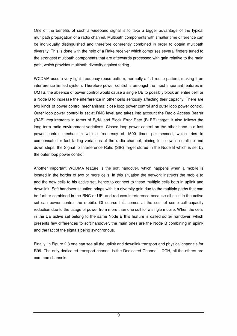
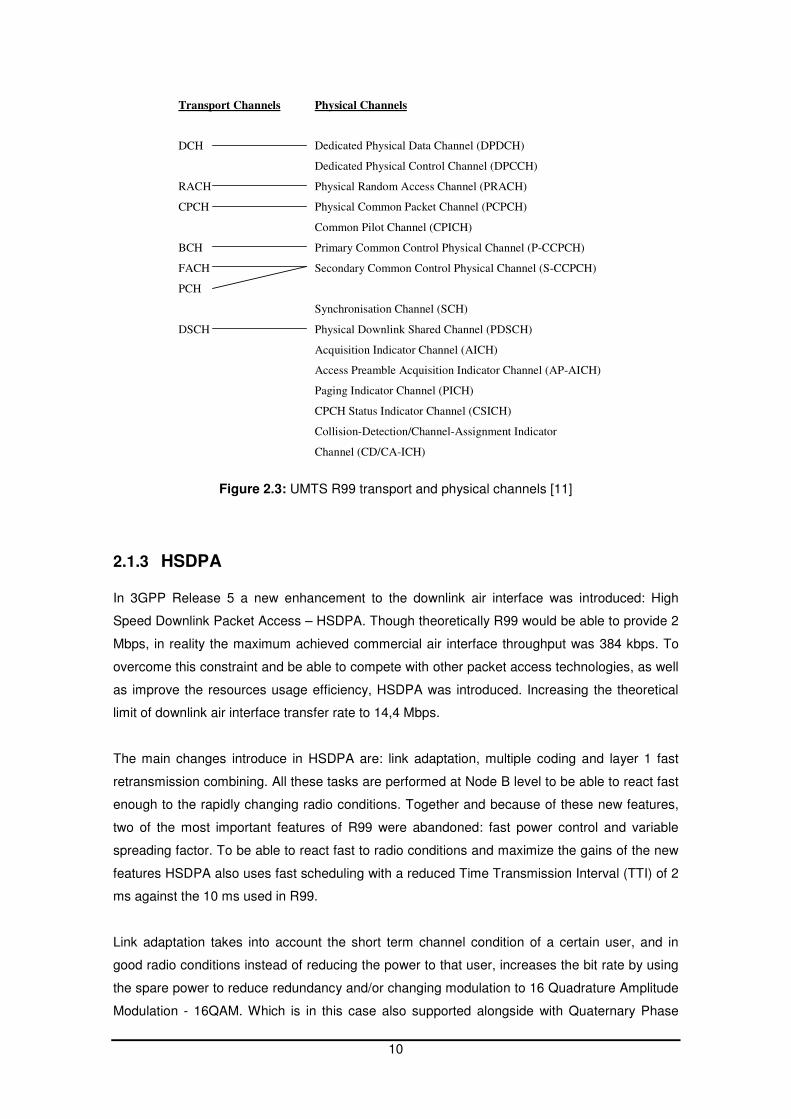
Finally, in Figure 2.3 one can see all the uplink and downlink transport and physical channels for
R99. The only dedicated transport channel is the Dedicated Channel - DCH, all the others are
common channels.
10
Transport Channels
DCH
RACH
CPCH
BCH
FACH
PCH
DSCH
Physical Channels
Dedicated Physical Data Channel (DPDCH)
Dedicated Physical Control Channel (DPCCH)
Physical Random Access Channel (PRACH)
Physical Common Packet Channel (PCPCH)
Common Pilot Channel (CPICH)
Primary Common Control Physical Channel (P-CCPCH)
Secondary Common Control Physical Channel (S-CCPCH)
Synchronisation Channel (SCH)
Physical Downlink Shared Channel (PDSCH)
Acquisition Indicator Channel (AICH)
Access Preamble Acquisition Indicator Channel (AP-AICH)
Paging Indicator Channel (PICH)
CPCH Status Indicator Channel (CSICH)
Collision-Detection/Channel-Assignment Indicator
Channel (CD/CA-ICH)
Figure 2.3: UMTS R99 transport and physical channels [11]
2.1.3 HSDPA In 3GPP Release 5 a new enhancement to the downlink air interface was introduced: High
Speed Downlink Packet Access – HSDPA. Though theoretically R99 would be able to provide 2
Mbps, in reality the maximum achieved commercial air interface throughput was 384 kbps. To
overcome this constraint and be able to compete with other packet access technologies, as well
as improve the resources usage efficiency, HSDPA was introduced. Increasing the theoretical
limit of downlink air interface transfer rate to 14,4 Mbps.
The main changes introduce in HSDPA are: link adaptation, multiple coding and layer 1 fast
retransmission combining. All these tasks are performed at Node B level to be able to react fast
enough to the rapidly changing radio conditions. Together and because of these new features,
two of the most important features of R99 were abandoned: fast power control and variable
spreading factor. To be able to react fast to radio conditions and maximize the gains of the new
features HSDPA also uses fast scheduling with a reduced Time Transmission Interval (TTI) of 2
ms against the 10 ms used in R99.
Link adaptation takes into account the short term channel condition of a certain user, and in
good radio conditions instead of reducing the power to that user, increases the bit rate by using
the spare power to reduce redundancy and/or changing modulation to 16 Quadrature Amplitude
Modulation - 16QAM. Which is in this case also supported alongside with Quaternary Phase
11
Shift Keying - QPSK. Moreover in HSDPA if a user requires higher bit rates the SF is not
reduced but he is assigned with multiple SF16 codes, which is the only spreading factor
supported. Depending on the cell and mobile capacity up to 15 codes can be assigned to a
single user.
HSDPA also uses Layer 1 fast retransmission combining based on the Hybrid Automatic
Repeat Request (HARQ) functionality. HARQ functionality works with parallel processes for
consecutive TTIs and it is based on Cyclic Redundancy Checks (CRC) on the UE that send
back to the Node B a positive (ACK) or negative (NACK) acknowledgement . With this
information the Node B schedules again for transmission, for a maximum number of times, the
data which feedback was a NACK. The retransmission mechanism could be based on Chase
combining or Incremental redundancy. The first simply retransmits the same information in the
event of a NACK, whilst the second saves the received bits in a buffer and ask for
retransmission of bits not sent in the first place.
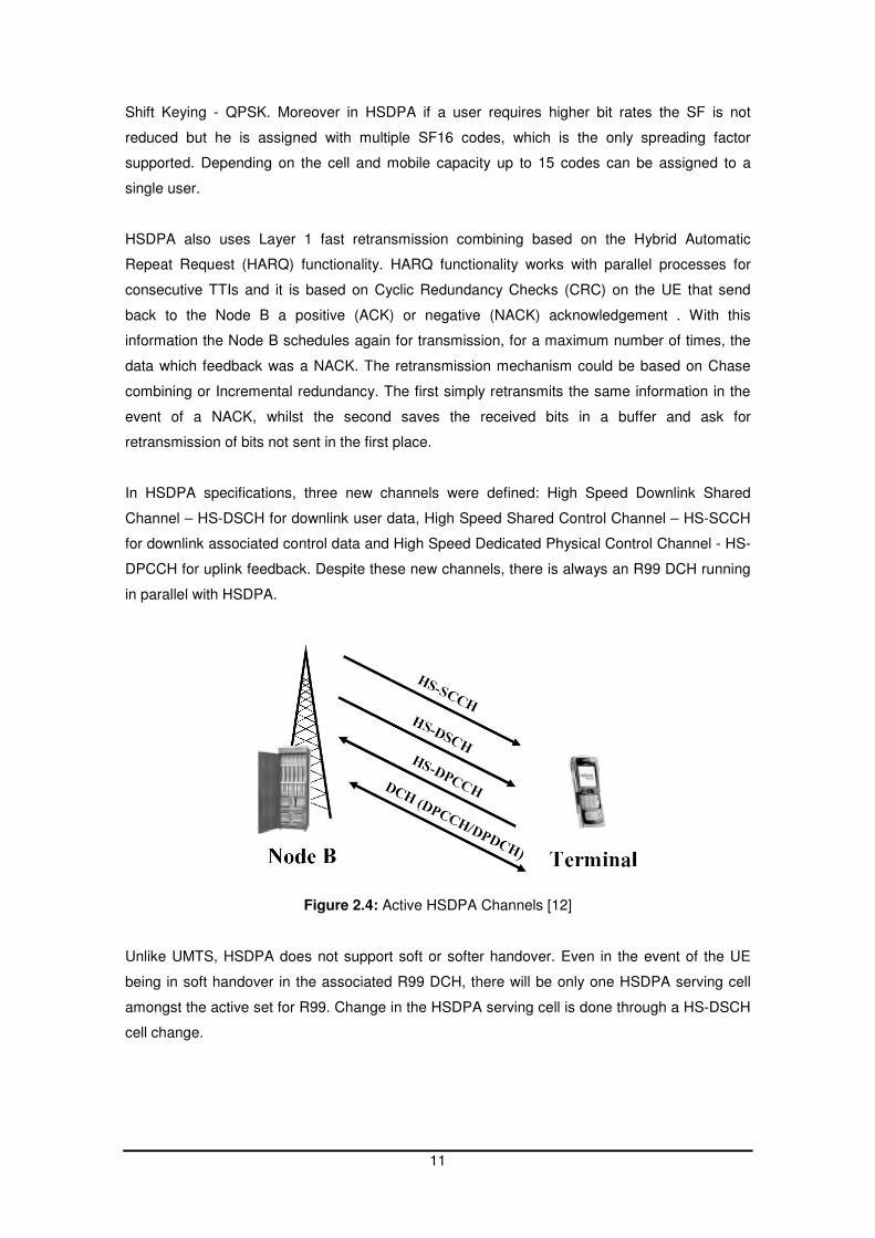
In HSDPA specifications, three new channels were defined: High Speed Downlink Shared
Channel – HS-DSCH for downlink user data, High Speed Shared Control Channel – HS-SCCH
for downlink associated control data and High Speed Dedicated Physical Control Channel - HS-
DPCCH for uplink feedback. Despite these new channels, there is always an R99 DCH running
in parallel with HSDPA.
Figure 2.4: Active HSDPA Channels [12]
Unlike UMTS, HSDPA does not support soft or softer handover. Even in the event of the UE
being in soft handover in the associated R99 DCH, there will be only one HSDPA serving cell
amongst the active set for R99. Change in the HSDPA serving cell is done through a HS-DSCH
cell change.
12
2.2 HSUPA Description Though most of the packet services still require faster download rates than upload, more and
more applications require high upload bit rates as well. After the specification of HSDPA, 3GPP
turned their attention to the radio uplink performance in order to get an improved user
experience. The result of this effort was a set of specifications for Enhanced Uplink; commonly
know as High Speed Uplink Packet Access, HSUPA.
2.2.1 HSUPA Features and Channels
Due to the differences between uplink and downlink, it was not possible to replicate all HSDPA
techniques in HSUPA. Actually HSUPA does not introduce major changes to UMTS basic
features. There are three main differences from HSUPA to R99: fast Node B based scheduling,
fast physical layer HARQ and optional 2ms TTI. All these features are supported in a new uplink
transport channel, Enhanced Dedicated Channel (E-DCH).
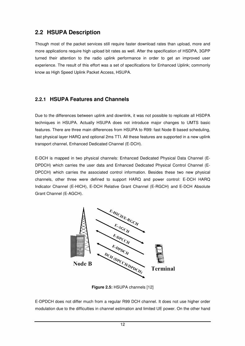
E-DCH is mapped in two physical channels: Enhanced Dedicated Physical Data Channel (E-
DPDCH) which carries the user data and Enhanced Dedicated Physical Control Channel (E-
DPCCH) which carries the associated control information. Besides these two new physical
channels, other three were defined to support HARQ and power control: E-DCH HARQ
Indicator Channel (E-HICH), E-DCH Relative Grant Channel (E-RGCH) and E-DCH Absolute
Grant Channel (E-AGCH).
Figure 2.5: HSUPA channels [12]
E-DPDCH does not differ much from a regular R99 DCH channel. It does not use higher order
modulation due to the difficulties in channel estimation and limited UE power. On the other hand
13
fast power control is used in order to avoid the near-far effect, and also to control interference
soft and softer handover is also used. To serve different data rates variable SF is employed and
one of the improvements of HSUPA towards R99 is the introduction of SF2. By using I and Q
branches of the transmitter a maximum of 2 x SF2 + 2 x SF4 can be utilized. Nevertheless only
one E-DCH per UE can be configured, though multiple applications can be multiplexed in it at
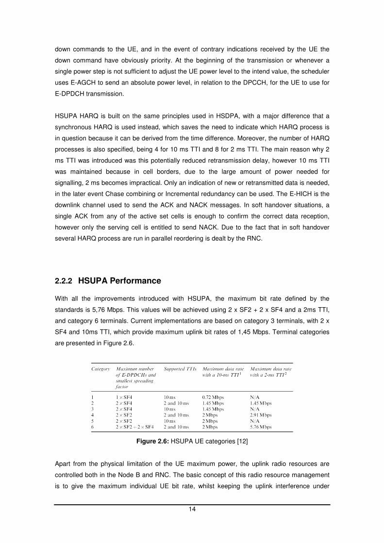
higher layers. Table 2.2 presents a summary of the main characteristics of E-DPDCH and the
Dedicated Physical Data Channel - DPDCH.
Table 2.2: DPDCH and E-DPDCH comparison [12]
E-DPCCH consists of a 10 bit information block which is sent over in 2 ms intervals using
SF256. In the case of 10 ms TTI the same information is sent 5 times with less power. For every
E-DPDCH there is an associated E-DPCCH which transmits the information needed for the
receiver to properly decode the subsequent associated E-DPDCH, the 7 bit E-DCH Transport
Format Indicator (E-TFCI). Besides that also transmits information needed for HARQ, the 2 bit
retransmission sequence number and the happy bit which informs whether the mobile is
satisfied with his currently allocated data rate.
Like HSDPA the scheduling was moved to the Node B. However the scheduler does not
manage power in a shared channel to all users, instead it manages the total cell noise rise
generated by individual dedicated channels from each user, which have their own individual
power allowance. All users have simultaneous access to the cell at predefined maximum data
rate, and the scheduler task is to downgrade existent users in order to accommodate new users
and to avoid reaching the maximum allowed noise rise in the cell. This scheduling behaviour is
not much different from R99 though the location of the scheduler in the Node B enables a much
faster adaptation to the current uplink interference situation.
To control the power for each individual user the Node B uses the downlink E-RGCH. E-RGCH
uses SF128 and depending on the cell load and UE capabilities can present 3 different values:
up, down and hold. In the event of an up or down command the UE adjusts its output power by
one step and consequently its uplink data rate. Cells outside the UE active set can also send
14
down commands to the UE, and in the event of contrary indications received by the UE the
down command have obviously priority. At the beginning of the transmission or whenever a
single power step is not sufficient to adjust the UE power level to the intend value, the scheduler
uses E-AGCH to send an absolute power level, in relation to the DPCCH, for the UE to use for
E-DPDCH transmission.
HSUPA HARQ is built on the same principles used in HSDPA, with a major difference that a
synchronous HARQ is used instead, which saves the need to indicate which HARQ process is
in question because it can be derived from the time difference. Moreover, the number of HARQ
processes is also specified, being 4 for 10 ms TTI and 8 for 2 ms TTI. The main reason why 2
ms TTI was introduced was this potentially reduced retransmission delay, however 10 ms TTI
was maintained because in cell borders, due to the large amount of power needed for
signalling, 2 ms becomes impractical. Only an indication of new or retransmitted data is needed,
in the later event Chase combining or Incremental redundancy can be used. The E-HICH is the
downlink channel used to send the ACK and NACK messages. In soft handover situations, a
single ACK from any of the active set cells is enough to confirm the correct data reception,
however only the serving cell is entitled to send NACK. Due to the fact that in soft handover
several HARQ process are run in parallel reordering is dealt by the RNC.
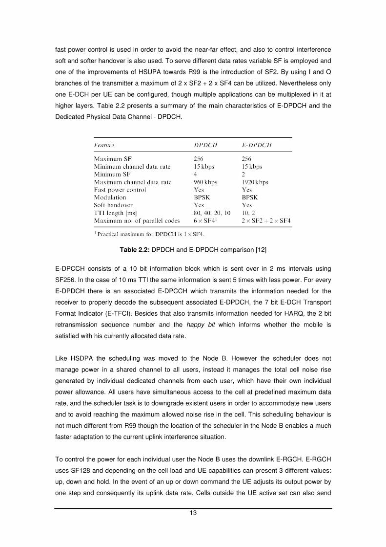
2.2.2 HSUPA Performance With all the improvements introduced with HSUPA, the maximum bit rate defined by the
standards is 5,76 Mbps. This values will be achieved using 2 x SF2 + 2 x SF4 and a 2ms TTI,
and category 6 terminals. Current implementations are based on category 3 terminals, with 2 x
SF4 and 10ms TTI, which provide maximum uplink bit rates of 1,45 Mbps. Terminal categories
are presented in Figure 2.6.
Figure 2.6: HSUPA UE categories [12]
Apart from the physical limitation of the UE maximum power, the uplink radio resources are
controlled both in the Node B and RNC. The basic concept of this radio resource management
is to give the maximum individual UE bit rate, whilst keeping the uplink interference under

15
control. The RNC is responsible by the resource allocation and admission control, whilst Node B
controls the packet scheduling.
RNC sets a target value for the maximum received total wideband power, which is equivalent to
establish a maximum noise rise (NR) or the amount of total uplink interference with respect to a
completely unloaded and isolated cell. This noise floor is determined by the sum of thermal
noise and receiver noise. However not all the available noise rise can be used by E-DCH,
actually E-DCH has always the least priority and only uses the spare noise rise. First of all a
part of the noise rise is consumed by inter-cell interference, which is obviously not controlled by
the serving cell. On top of this, all DCH R99 connections have priority over E-DCH, mainly
because it carries all the CS connections which are more sensitive to rate variations.
Nevertheless in cells with HSUPA active, R99 DCH is limited to 64 kbps. The generic noise rise
distribution is presented in Figure 2.7.
Figure 2.7: Noise rise distribution [12]
The RNC controls the scheduling of non E-DCH channels and informs the Node B about the
amount of interference rise it has available to schedule E-DCH channels from the different UE.
The RNC is also responsible for the Admission Control, including for E-DCH, it basically checks
if a new user in the system will not exceed the maximum pre-defined interference level. It takes
also into account the incoming request Scheduling Priority Indicator (SPI) or if the new request
is for a guaranteed bit rate service, these could lead to a downgrade in one of the existing
connections. On top of that it has to check if the maximum number of active HSUPA users was
not reached and if there are enough HSDPA resources for that user, because HSUPA requires
the usage of HSDPA in the downlink.
As stated previously the Node B is responsible for scheduling the remainder noise rise for E-
DCH connections. This is one of the advantages of the HSUPA, due to the fact that the
scheduler is closer to the air interface it has a better knowledge of the instantaneous
interference permitting faster scheduling, which allows higher load and throughputs. This
scheduling is done taking under consideration three main parameters: the available UE power,
the UE buffer status and the happy bit.
16
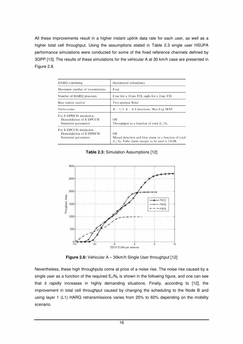
All these improvements result in a higher instant uplink data rate for each user, as well as a
higher total cell throughput. Using the assumptions stated in Table 2.3 single user HSUPA
performance simulations were conducted for some of the fixed reference channels defined by
3GPP [13]. The results of these simulations for the vehicular A at 30 km/h case are presented in
Figure 2.8.
Table 2.3: Simulation Assumptions [12]
Figure 2.8: Vehicular A – 30km/h Single User throughput [12]
Nevertheless, these high throughputs come at price of a noise rise. The noise rise caused by a
single user as a function of the required Ec/N0 is shown in the following figure, and one can see
that it rapidly increases in highly demanding situations. Finally, according to [12], the
improvement in total cell throughput caused by changing the scheduling to the Node B and
using layer 1 (L1) HARQ retransmissions varies from 25% to 60% depending on the mobility
scenario.
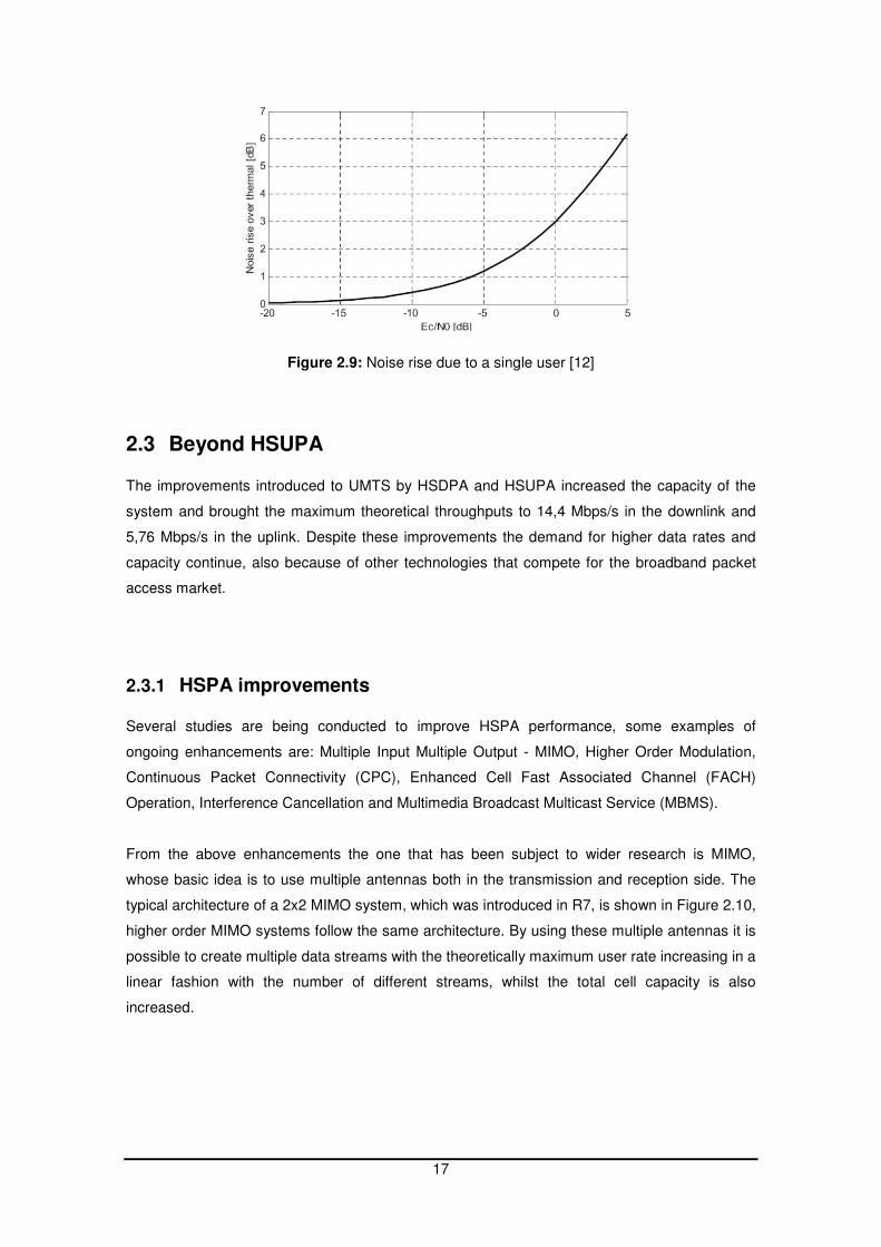
17
Figure 2.9: Noise rise due to a single user [12]
2.3 Beyond HSUPA The improvements introduced to UMTS by HSDPA and HSUPA increased the capacity of the
system and brought the maximum theoretical throughputs to 14,4 Mbps/s in the downlink and
5,76 Mbps/s in the uplink. Despite these improvements the demand for higher data rates and
capacity continue, also because of other technologies that compete for the broadband packet
access market.
2.3.1 HSPA improvements Several studies are being conducted to improve HSPA performance, some examples of
ongoing enhancements are: Multiple Input Multiple Output - MIMO, Higher Order Modulation,
Continuous Packet Connectivity (CPC), Enhanced Cell Fast Associated Channel (FACH)
Operation, Interference Cancellation and Multimedia Broadcast Multicast Service (MBMS).
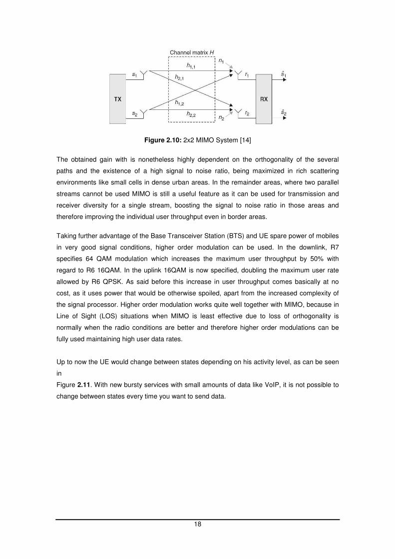
From the above enhancements the one that has been subject to wider research is MIMO,
whose basic idea is to use multiple antennas both in the transmission and reception side. The
typical architecture of a 2x2 MIMO system, which was introduced in R7, is shown in Figure 2.10,
higher order MIMO systems follow the same architecture. By using these multiple antennas it is
possible to create multiple data streams with the theoretically maximum user rate increasing in a
linear fashion with the number of different streams, whilst the total cell capacity is also
increased.
18
Figure 2.10: 2x2 MIMO System [14]
The obtained gain with is nonetheless highly dependent on the orthogonality of the several
paths and the existence of a high signal to noise ratio, being maximized in rich scattering
environments like small cells in dense urban areas. In the remainder areas, where two parallel
streams cannot be used MIMO is still a useful feature as it can be used for transmission and
receiver diversity for a single stream, boosting the signal to noise ratio in those areas and
therefore improving the individual user throughput even in border areas.
Taking further advantage of the Base Transceiver Station (BTS) and UE spare power of mobiles
in very good signal conditions, higher order modulation can be used. In the downlink, R7
specifies 64 QAM modulation which increases the maximum user throughput by 50% with
regard to R6 16QAM. In the uplink 16QAM is now specified, doubling the maximum user rate
allowed by R6 QPSK. As said before this increase in user throughput comes basically at no
cost, as it uses power that would be otherwise spoiled, apart from the increased complexity of
the signal processor. Higher order modulation works quite well together with MIMO, because in
Line of Sight (LOS) situations when MIMO is least effective due to loss of orthogonality is
normally when the radio conditions are better and therefore higher order modulations can be
fully used maintaining high user data rates.
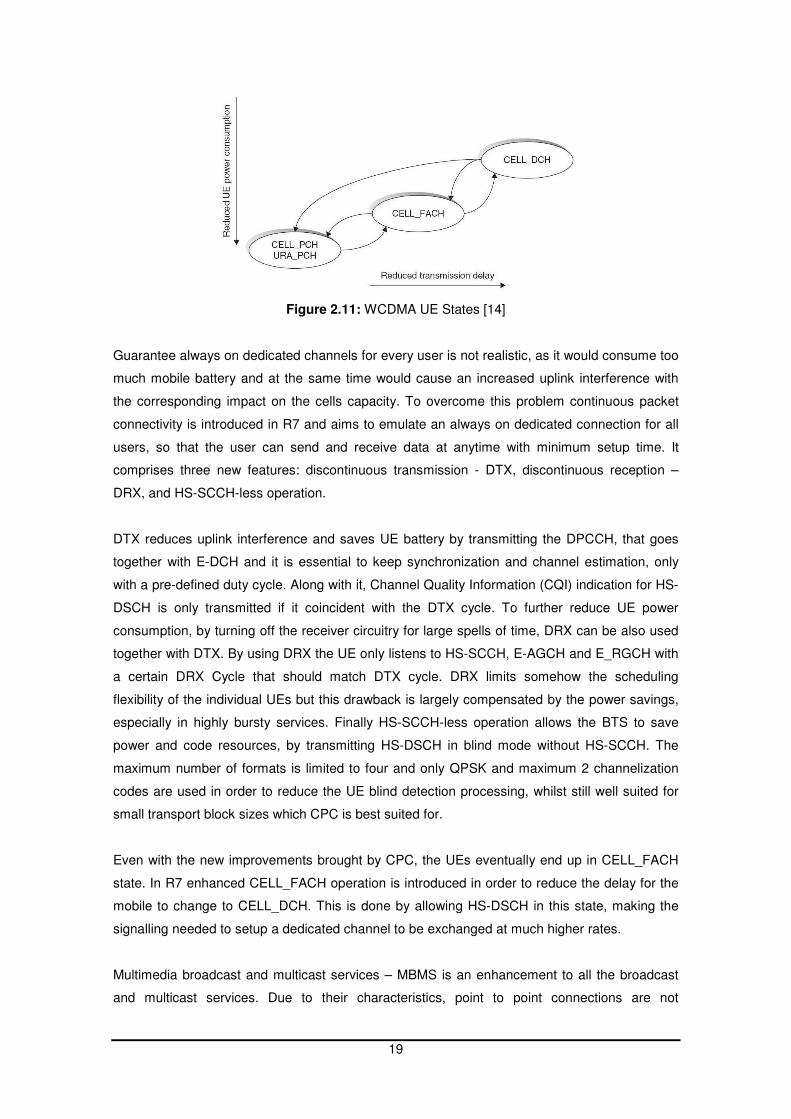
Up to now the UE would change between states depending on his activity level, as can be seen
in
Figure 2.11. With new bursty services with small amounts of data like VoIP, it is not possible to
change between states every time you want to send data.
19
Figure 2.11: WCDMA UE States [14]
Guarantee always on dedicated channels for every user is not realistic, as it would consume too
much mobile battery and at the same time would cause an increased uplink interference with
the corresponding impact on the cells capacity. To overcome this problem continuous packet
connectivity is introduced in R7 and aims to emulate an always on dedicated connection for all
users, so that the user can send and receive data at anytime with minimum setup time. It
comprises three new features: discontinuous transmission - DTX, discontinuous reception –
DRX, and HS-SCCH-less operation.
DTX reduces uplink interference and saves UE battery by transmitting the DPCCH, that goes
together with E-DCH and it is essential to keep synchronization and channel estimation, only
with a pre-defined duty cycle. Along with it, Channel Quality Information (CQI) indication for HS-
DSCH is only transmitted if it coincident with the DTX cycle. To further reduce UE power
consumption, by turning off the receiver circuitry for large spells of time, DRX can be also used
together with DTX. By using DRX the UE only listens to HS-SCCH, E-AGCH and E_RGCH with
a certain DRX Cycle that should match DTX cycle. DRX limits somehow the scheduling
flexibility of the individual UEs but this drawback is largely compensated by the power savings,
especially in highly bursty services. Finally HS-SCCH-less operation allows the BTS to save
power and code resources, by transmitting HS-DSCH in blind mode without HS-SCCH. The
maximum number of formats is limited to four and only QPSK and maximum 2 channelization
codes are used in order to reduce the UE blind detection processing, whilst still well suited for
small transport block sizes which CPC is best suited for.
Even with the new improvements brought by CPC, the UEs eventually end up in CELL_FACH
state. In R7 enhanced CELL_FACH operation is introduced in order to reduce the delay for the
mobile to change to CELL_DCH. This is done by allowing HS-DSCH in this state, making the
signalling needed to setup a dedicated channel to be exchanged at much higher rates.
Multimedia broadcast and multicast services – MBMS is an enhancement to all the broadcast
and multicast services. Due to their characteristics, point to point connections are not
20
appropriate to serve broadcast or multicast services because they use resources inefficiently by
sending the same information over and over again to different users. On the other hand
broadcast services have no feedback from users but must be able to reach them despite their
location within the cell, therefore broadcast channels should be transmitted with high power.
With MBMS the packets are only sent once, as in normal broadcast, and all the interested UEs
receive that information, saving valuable resources comparing with point to point connections.
Moreover, same data is sent via several cells, which allows the UE to receive the different
signals and combine them to obtain a gain towards single path transmission. Therefore the
broadcast channels can be transmitted by the network at lower power because UEs in border
locations will benefit from this multipath transmission. Finally with MBMS, TTI is increased and
application level coding is introduced in order mitigate the fast fading effects in the radio
channel.
2.3.2 LTE basics
Besides the work on the new UMTS releases, 3GPP is following a parallel path in the
development of more capable mobile broadband access technologies with 3G Long Term
Evolution, commonly known as LTE. The goal for LTE in terms of peak data rate in the air
interface is 100 Mbps in the downlink and 50 Mbps in the uplink, considering a 20 MHz
bandwidth.
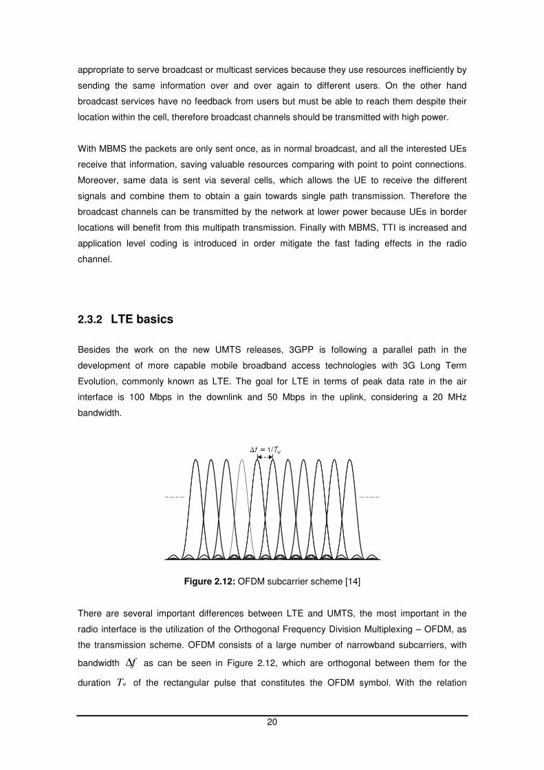
Figure 2.12: OFDM subcarrier scheme [14]
There are several important differences between LTE and UMTS, the most important in the
radio interface is the utilization of the Orthogonal Frequency Division Multiplexing – OFDM, as
the transmission scheme. OFDM consists of a large number of narrowband subcarriers, with
bandwidth f∆ as can be seen in Figure 2.12, which are orthogonal between them for the
duration uT of the rectangular pulse that constitutes the OFDM symbol. With the relation
21
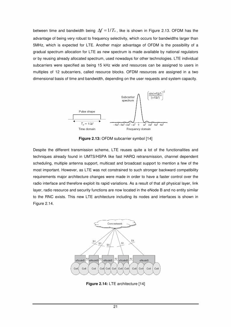
between time and bandwidth being uTf /1=∆ , like is shown in Figure 2.13. OFDM has the
advantage of being very robust to frequency selectivity, which occurs for bandwidths larger than
5MHz, which is expected for LTE. Another major advantage of OFDM is the possibility of a
gradual spectrum allocation for LTE as new spectrum is made available by national regulators
or by reusing already allocated spectrum, used nowadays for other technologies. LTE individual
subcarriers were specified as being 15 kHz wide and resources can be assigned to users in
multiples of 12 subcarriers, called resource blocks. OFDM resources are assigned in a two
dimensional basis of time and bandwidth, depending on the user requests and system capacity.
Figure 2.13: OFDM subcarrier symbol [14]
Despite the different transmission scheme, LTE reuses quite a lot of the functionalities and
techniques already found in UMTS/HSPA like fast HARQ retransmission, channel dependent
scheduling, multiple antenna support, multicast and broadcast support to mention a few of the
most important. However, as LTE was not constrained to such stronger backward compatibility
requirements major architecture changes were made in order to have a faster control over the
radio interface and therefore exploit its rapid variations. As a result of that all physical layer, link
layer, radio resource and security functions are now located in the eNode B and no entity similar
to the RNC exists. This new LTE architecture including its nodes and interfaces is shown in
Figure 2.14.
Figure 2.14: LTE architecture [14]

22
23
3 Test Scenarios
This chapter presents a full description of the test scenarios together with a theoretical
approach to HSUPA performance in the various indoor situations. First a general presentation
of the test methodologies and a theoretical approach to indoor coverage and capacity is
presented. The next subchapter deals with indoor coverage provided by outdoor sites, which is
by far the most common situation. Whilst in 3.3 indoor environments with dedicated BTSs and
passive distributed antenna systems are presented. Finally in 3.4 the use of RF and optical
repeaters indoors is discussed.
24
3.1 Introduction
In the former chapters only general characteristics of HSUPA were subject to analysis. In this
chapter the different indoor test scenarios and methodologies, which are the main subject of this
document, will be described in detail, stressing their differentiating characteristics. Also a more
detailed analysis of the HSUPA performance in the different indoor environments will be
presented. The chapter is divided in four main blocks; the first one describes the test
methodology whilst the remaining three are dedicated to the different indoor test scenarios:
coverage by regular outdoor sites, dedicated BTSs based on passive distributed antenna
systems and finally RF and fibre optics repeaters.
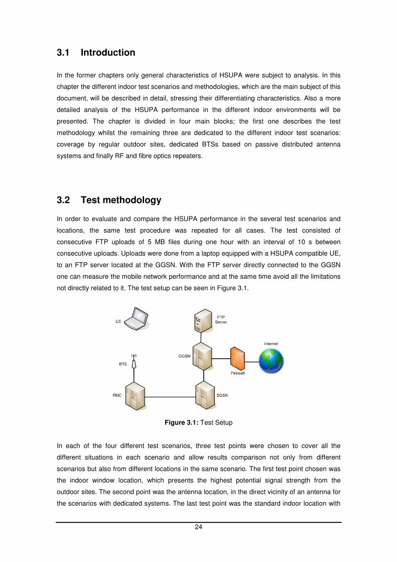
3.2 Test methodology In order to evaluate and compare the HSUPA performance in the several test scenarios and
locations, the same test procedure was repeated for all cases. The test consisted of
consecutive FTP uploads of 5 MB files during one hour with an interval of 10 s between
consecutive uploads. Uploads were done from a laptop equipped with a HSUPA compatible UE,
to an FTP server located at the GGSN. With the FTP server directly connected to the GGSN
one can measure the mobile network performance and at the same time avoid all the limitations
not directly related to it. The test setup can be seen in Figure 3.1.
Figure 3.1: Test Setup
In each of the four different test scenarios, three test points were chosen to cover all the
different situations in each scenario and allow results comparison not only from different
scenarios but also from different locations in the same scenario. The first test point chosen was
the indoor window location, which presents the highest potential signal strength from the
outdoor sites. The second point was the antenna location, in the direct vicinity of an antenna for
the scenarios with dedicated systems. The last test point was the standard indoor location with
25
no line of sight with any antenna and at least one wall between the closest antenna and the
mobile. For the outdoor site scenario a deep indoor location replaced the antenna location. For
all the combinations of scenarios and test points, several metrics were collected, namely:
Received Signal Code Power - RSCP [dBm], Energy per chip over interference density - Ec/I0
[dB], Uplink bit rate [kbps] and BTS received total wideband power [dB].
3.3 Coverage and capacity
HSUPA coverage can be obtained trough link budget calculations. Examples of link budget
calculations for UMTS can be easily found in the literature, as for example in [15]. However
there are several changes in link budget introduced by HSUPA, namely: different and variable
information rate, increased NR target, modified Eb/N0 requirements.
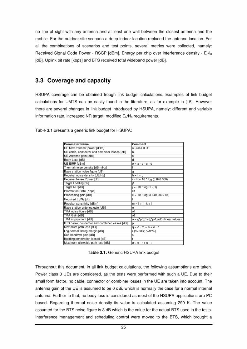
Table 3.1 presents a generic link budget for HSUPA:
Parameter Name Comment
UE Max transmit power [dBm] a Class 3 UE
UE cable, connector and combiner losses [dB] b
UE Antenna gain [dBi] c
Body Loss [dB] d
UE EIRP [dBm] e = a - b - c - d
Thermal noise density [dBm/Hz] f
Base station noise figure [dB] g
Receiver noise density [dB/Hz] h = f + g
Receiver Noise Power [dB] i = h + 10 * log (3 840 000)
Target Loading [%] j1
Target NR [dB] j = -10 * log (1 - j1)
Information Rate [Kbps] k1
Processing gain [dB] k = 10 * log (3 840 000 / k1)
Required Eb/N0 [dB] l
Receiver sensitivity [dBm] m = i + j - k + l
Base station antenna gain [dBi] n
TMA noise figure [dB] o1
TMA Gain [dB] o2
TMA improvment [dB] o = g*p/(o1+(g*p-1)/o2) (linear values)
BTS cable, connector and combiner losses [dB] p
Maximum path loss [dB] q = e - m + n + o - p
Log-normal fading margin [dB] r (σ=8dB; p=95%)
Soft handover gain [dB] s
Building penetration losses [dB] t
Maximum allowable path loss [dB] u = q - r + s - t
Table 3.1: Generic HSUPA link budget
Throughout this document, in all link budget calculations, the following assumptions are taken.
Power class 3 UEs are considered, as the tests were performed with such a UE. Due to their
small form factor, no cable, connector or combiner losses in the UE are taken into account. The
antenna gain of the UE is assumed to be 0 dBi, which is normally the case for a normal internal
antenna. Further to that, no body loss is considered as most of the HSUPA applications are PC
based. Regarding thermal noise density its value is calculated assuming 290 K. The value
assumed for the BTS noise figure is 3 dB which is the value for the actual BTS used in the tests.
Interference management and scheduling control were moved to the BTS, which brought a
26
faster reaction to variations in the radio channel and therefore the system can handle higher cell
loads. In the link budget calculations a load value of 90% and a correspondent 10 dB noise rise
is considered, as it was the set value in the test cells. The Eb/N0 ratio considered in this
document is based on link level simulations, from [5], for the predefined 3GPP Pedestrian at 3
km/h channel, 10 ms TTI and 3 HARQ maximum retransmissions, with category 5 UE. The
current tests were performed with category 3 UEs, and not category 5 and due to that fact, no
results were presented for a 14484 Transport Block Size - TBS. Moreover PA3 channel is not
exactly the test scenario, as all the tests were performed in static positions. However, and
despite these differences, the described scenario is a good approximation to the current test
scenario and therefore the target Eb/N0 value of 3.44 dB, for the closest TBS value of 14202
from the simulations, was chosen as the best estimation to the link budget calculations.
In each scenario a specific link budget will be calculated taking into account the specific
equipment and radio characteristics of the different environments. Using the results of those link
budget calculations in an appropriate radio model will allow us to calculate the maximum cell
radius where HSUPA will be theoretically available.
Coverage and capacity are strongly related in UMTS. In HSUPA, despite the improvement in
spectral efficiency, still the amount of noise rise allowed at the BTS determines the maximum
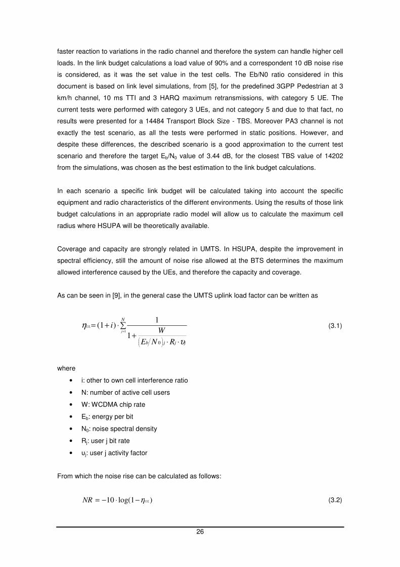
allowed interference caused by the UEs, and therefore the capacity and coverage.
As can be seen in [9], in the general case the UMTS uplink load factor can be written as
∑
⋅⋅+
⋅+==
N
jjjb
j
UL
RNE
Wi
1
0
1
1)(1
υ
η (3.1)
where
• i: other to own cell interference ratio
• N: number of active cell users
• W: WCDMA chip rate
• Eb: energy per bit
• N0: noise spectral density
• Rj: user j bit rate
• υj: user j activity factor
From which the noise rise can be calculated as follows:
)1log(10 ULNR η−⋅−= (3.2)
27
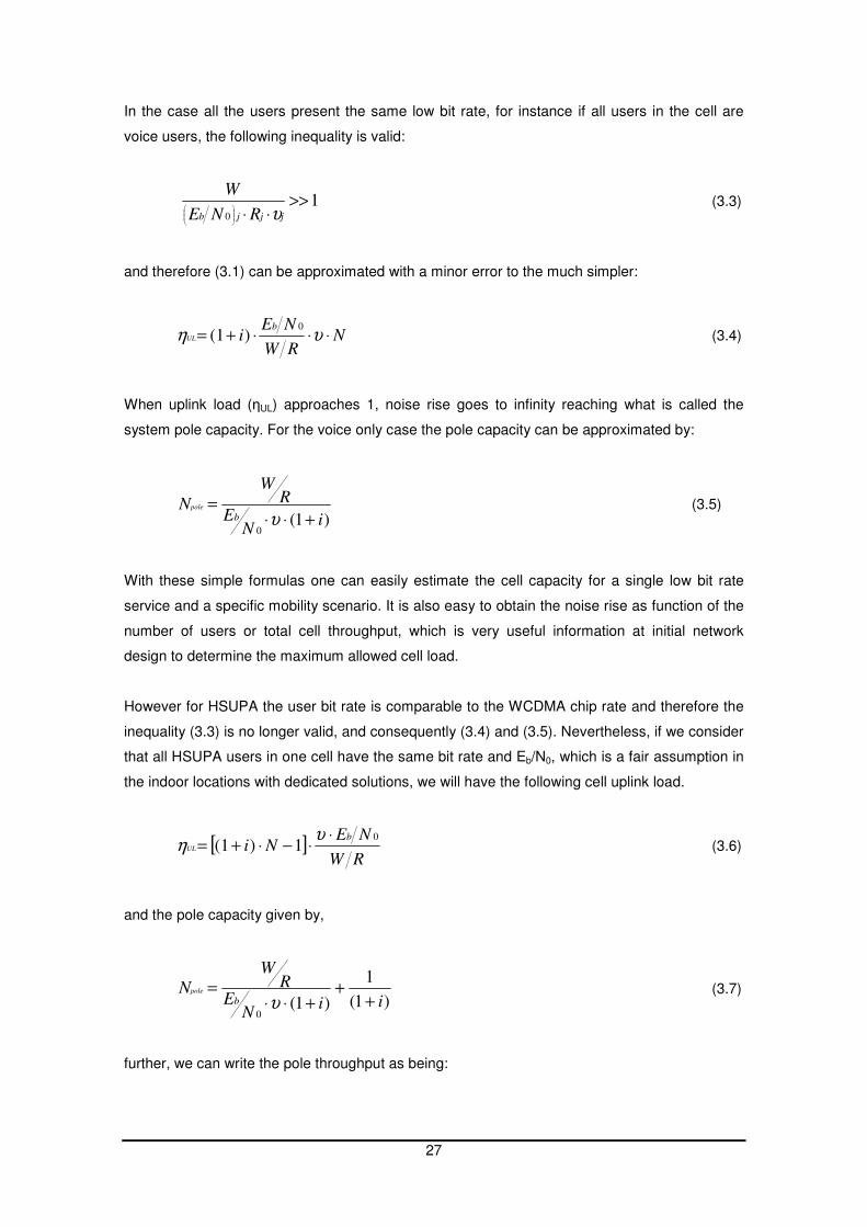
In the case all the users present the same low bit rate, for instance if all users in the cell are
voice users, the following inequality is valid:
10
>>⋅⋅
jjjb RNE
W
υ (3.3)
and therefore (3.1) can be approximated with a minor error to the much simpler:
NRW
NEi
bUL ⋅⋅⋅+= υη
0)(1 (3.4)
When uplink load (ηUL) approaches 1, noise rise goes to infinity reaching what is called the
system pole capacity. For the voice only case the pole capacity can be approximated by:
)1(
0i
NE
RW
Nb
pole
+⋅⋅=
υ (3.5)
With these simple formulas one can easily estimate the cell capacity for a single low bit rate
service and a specific mobility scenario. It is also easy to obtain the noise rise as function of the
number of users or total cell throughput, which is very useful information at initial network
design to determine the maximum allowed cell load.
However for HSUPA the user bit rate is comparable to the WCDMA chip rate and therefore the
inequality (3.3) is no longer valid, and consequently (3.4) and (3.5). Nevertheless, if we consider
that all HSUPA users in one cell have the same bit rate and Eb/N0, which is a fair assumption in
the indoor locations with dedicated solutions, we will have the following cell uplink load.
[ ]RW
NENi
bUL
01)(1
⋅⋅−⋅+=υ
η (3.6)
and the pole capacity given by,
)1(
1
)1(0
iiN
ER
W
Nb
pole
++
+⋅⋅=
υ (3.7)
further, we can write the pole throughput as being:
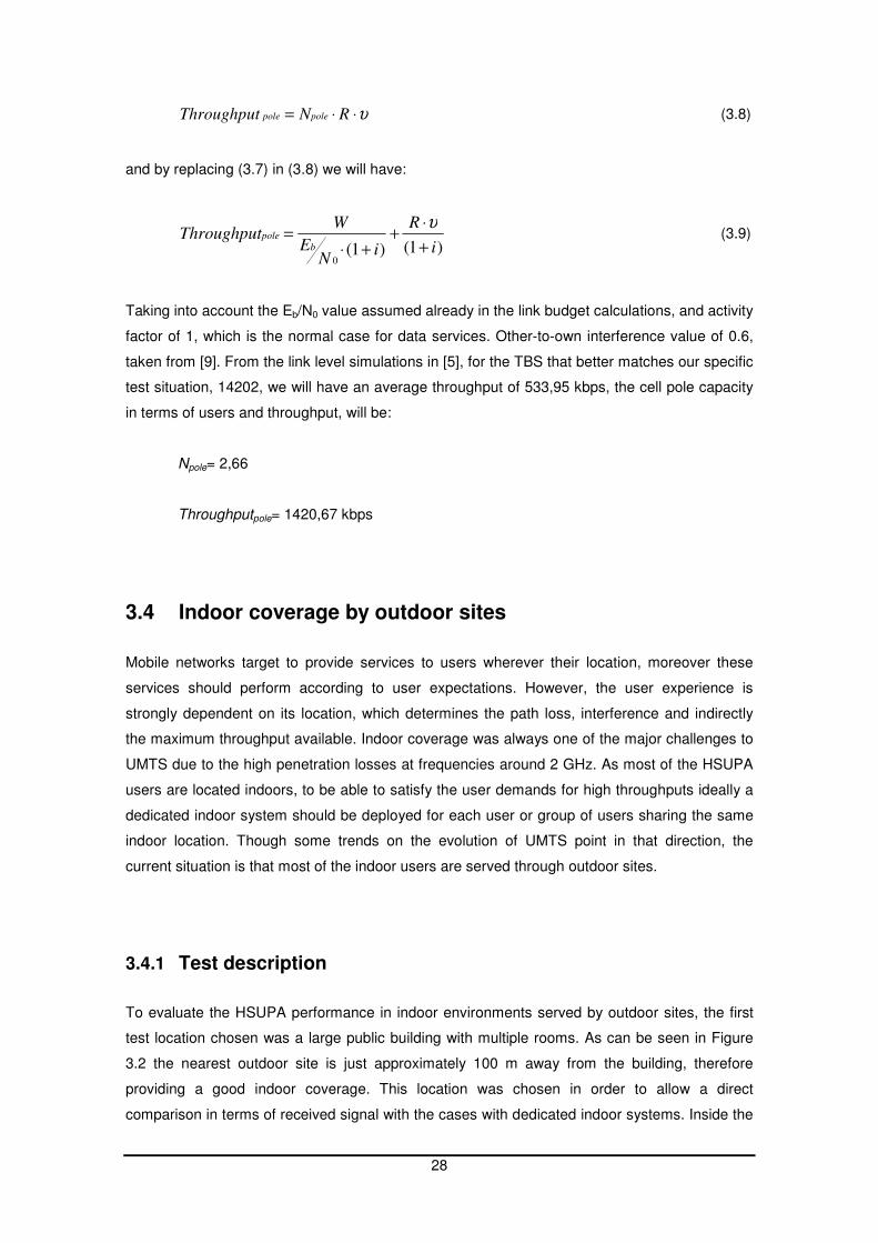
28
υ⋅⋅= RNThroughput polepole (3.8)
and by replacing (3.7) in (3.8) we will have:
)1()1(
0i
R
iN
E
WThroughput
b
pole
+
⋅+
+⋅=
υ (3.9)
Taking into account the Eb/N0 value assumed already in the link budget calculations, and activity
factor of 1, which is the normal case for data services. Other-to-own interference value of 0.6,
taken from [9]. From the link level simulations in [5], for the TBS that better matches our specific
test situation, 14202, we will have an average throughput of 533,95 kbps, the cell pole capacity
in terms of users and throughput, will be:
Npole= 2,66
Throughputpole= 1420,67 kbps
3.4 Indoor coverage by outdoor sites
Mobile networks target to provide services to users wherever their location, moreover these
services should perform according to user expectations. However, the user experience is
strongly dependent on its location, which determines the path loss, interference and indirectly
the maximum throughput available. Indoor coverage was always one of the major challenges to
UMTS due to the high penetration losses at frequencies around 2 GHz. As most of the HSUPA
users are located indoors, to be able to satisfy the user demands for high throughputs ideally a
dedicated indoor system should be deployed for each user or group of users sharing the same
indoor location. Though some trends on the evolution of UMTS point in that direction, the
current situation is that most of the indoor users are served through outdoor sites.
3.4.1 Test description
To evaluate the HSUPA performance in indoor environments served by outdoor sites, the first
test location chosen was a large public building with multiple rooms. As can be seen in Figure
3.2 the nearest outdoor site is just approximately 100 m away from the building, therefore
providing a good indoor coverage. This location was chosen in order to allow a direct
comparison in terms of received signal with the cases with dedicated indoor systems. Inside the
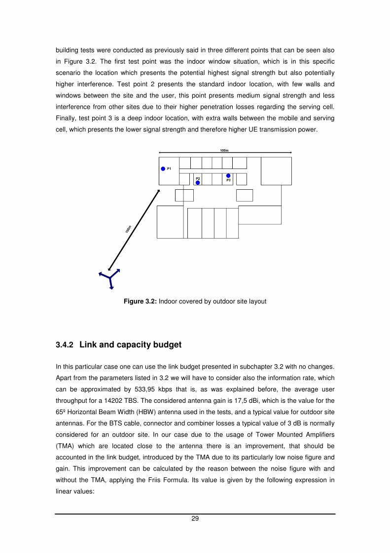
29
building tests were conducted as previously said in three different points that can be seen also
in Figure 3.2. The first test point was the indoor window situation, which is in this specific
scenario the location which presents the potential highest signal strength but also potentially
higher interference. Test point 2 presents the standard indoor location, with few walls and
windows between the site and the user, this point presents medium signal strength and less
interference from other sites due to their higher penetration losses regarding the serving cell.
Finally, test point 3 is a deep indoor location, with extra walls between the mobile and serving
cell, which presents the lower signal strength and therefore higher UE transmission power.
Figure 3.2: Indoor covered by outdoor site layout
3.4.2 Link and capacity budget
In this particular case one can use the link budget presented in subchapter 3.2 with no changes.
Apart from the parameters listed in 3.2 we will have to consider also the information rate, which
can be approximated by 533,95 kbps that is, as was explained before, the average user
throughput for a 14202 TBS. The considered antenna gain is 17,5 dBi, which is the value for the
65º Horizontal Beam Width (HBW) antenna used in the tests, and a typical value for outdoor site
antennas. For the BTS cable, connector and combiner losses a typical value of 3 dB is normally
considered for an outdoor site. In our case due to the usage of Tower Mounted Amplifiers
(TMA) which are located close to the antenna there is an improvement, that should be
accounted in the link budget, introduced by the TMA due to its particularly low noise figure and
gain. This improvement can be calculated by the reason between the noise figure with and
without the TMA, applying the Friis Formula. Its value is given by the following expression in
linear values:
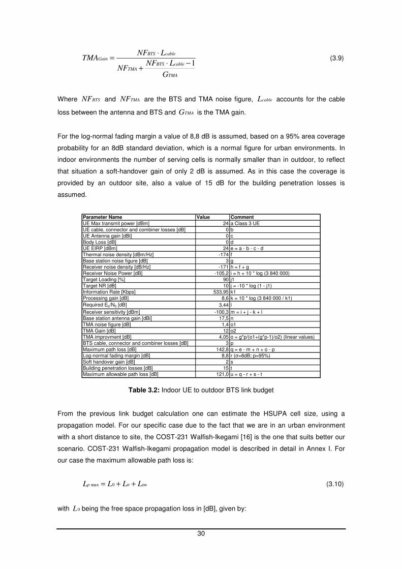
30
TMA
cableBTSTMA
cableBTSGain
G
LNFNF
LNFTMA
1−⋅+
⋅=
(3.9)
Where BTSNF and TMANF are the BTS and TMA noise figure, cableL accounts for the cable
loss between the antenna and BTS and TMAG is the TMA gain.
For the log-normal fading margin a value of 8,8 dB is assumed, based on a 95% area coverage
probability for an 8dB standard deviation, which is a normal figure for urban environments. In
indoor environments the number of serving cells is normally smaller than in outdoor, to reflect
that situation a soft-handover gain of only 2 dB is assumed. As in this case the coverage is
provided by an outdoor site, also a value of 15 dB for the building penetration losses is
assumed.
Parameter Name Value Comment
UE Max transmit power [dBm] 24 a Class 3 UE
UE cable, connector and combiner losses [dB] 0 b
UE Antenna gain [dBi] 0 c
Body Loss [dB] 0 d
UE EIRP [dBm] 24 e = a - b - c - d
Thermal noise density [dBm/Hz] -174 f
Base station noise figure [dB] 3 g
Receiver noise density [dB/Hz] -171 h = f + g
Receiver Noise Power [dB] -105,2 i = h + 10 * log (3 840 000)
Target Loading [%] 90 j1
Target NR [dB] 10 j = -10 * log (1 - j1)
Information Rate [Kbps] 533,95 k1
Processing gain [dB] 8,6 k = 10 * log (3 840 000 / k1)
Required Eb/N0 [dB] 3,44 l
Receiver sensitivity [dBm] -100,3 m = i + j - k + l
Base station antenna gain [dBi] 17,5 n
TMA noise figure [dB] 1,4 o1
TMA Gain [dB] 12 o2
TMA improvment [dB] 4,05 o = g*p/(o1+(g*p-1)/o2) (linear values)
BTS cable, connector and combiner losses [dB] 3 p
Maximum path loss [dB] 142,8 q = e - m + n + o - p
Log-normal fading margin [dB] 8,8 r (σ=8dB; p=95%)
Soft handover gain [dB] 2 s
Building penetration losses [dB] 15 t
Maximum allowable path loss [dB] 121,0 u = q - r + s - t
Table 3.2: Indoor UE to outdoor BTS link budget
From the previous link budget calculation one can estimate the HSUPA cell size, using a
propagation model. For our specific case due to the fact that we are in an urban environment
with a short distance to site, the COST-231 Walfish-Ikegami [16] is the one that suits better our
scenario. COST-231 Walfish-Ikegami propagation model is described in detail in Annex I. For
our case the maximum allowable path loss is:
tmttp LLLL ++= 0max (3.10)
with 0L being the free space propagation loss in [dB], given by:
31
)log(20)log(204.320 fRL ⋅+⋅+= (3.11)
where R is the cell radius in [km] and f the frequency in [MHz]. One the other hand ttL
accounts for the multi screen diffraction loss, and is calculated by:
)log(9)log()log( bfdabshtt wfKRKKLL ⋅−⋅+⋅++= (3.12)
Being bw =50 the building separation in [m], aK = 54 and dK = 18 in our particular case and
bshL obtained by the following expression:
)1log(18 +−⋅−= BBbsh hHL (3.13)
where BH =40 is the Node B antenna height and Bh =25 is the mean building height, both in
[m]. Finally tmL which accounts for the rooftop to UE diffraction and scatter loss, is calculated
by the following expression:
orimBStm LhHfwL +−⋅+⋅+⋅−−= )log(20)log(10)log(109.16 (3.14)
in which Sw =30 is the street width in [m], mh =1,5 the UE height in [m] and oriL is in our case,
considering the incidence angle from the BTS in the street ψ =90º, given by:
)55(114.04 −⋅−= ψoriL (3.15)
By replacing in (3.10) the maximum allowable path loss value calculated in Table 3.2, and
assuming its value as a good approximation for the current scenario, one will obtain a maximum
HSUPA cell radius of 0,355 km. This result confirms that we should expect HSUPA to be used
in the tests, as they were performed within the distance calculated as maximum for this service.
Regarding the capacity budget, this scenario totally reproduces the assumptions and values
assumed in 3.2 for its calculation. Therefore we should expect the values calculated there for
pole capacity, Npole= 2,66 and Throughputpole= 1420,67 kbps, to be considered valid.
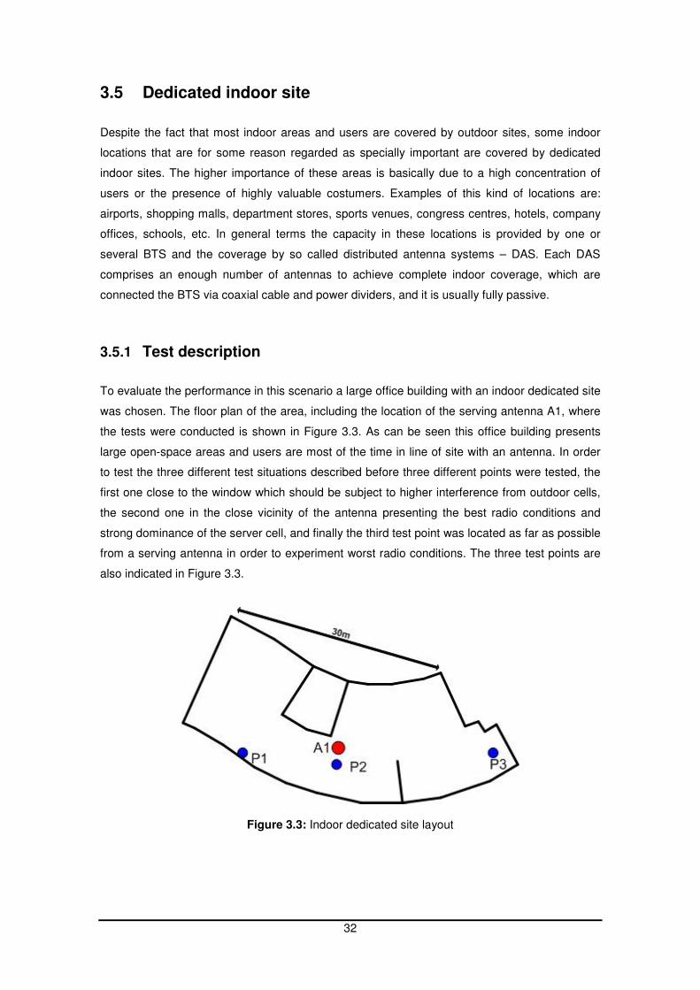
32
3.5 Dedicated indoor site
Despite the fact that most indoor areas and users are covered by outdoor sites, some indoor
locations that are for some reason regarded as specially important are covered by dedicated
indoor sites. The higher importance of these areas is basically due to a high concentration of
users or the presence of highly valuable costumers. Examples of this kind of locations are:
airports, shopping malls, department stores, sports venues, congress centres, hotels, company
offices, schools, etc. In general terms the capacity in these locations is provided by one or
several BTS and the coverage by so called distributed antenna systems – DAS. Each DAS
comprises an enough number of antennas to achieve complete indoor coverage, which are
connected the BTS via coaxial cable and power dividers, and it is usually fully passive.
3.5.1 Test description
To evaluate the performance in this scenario a large office building with an indoor dedicated site
was chosen. The floor plan of the area, including the location of the serving antenna A1, where
the tests were conducted is shown in Figure 3.3. As can be seen this office building presents
large open-space areas and users are most of the time in line of site with an antenna. In order
to test the three different test situations described before three different points were tested, the
first one close to the window which should be subject to higher interference from outdoor cells,
the second one in the close vicinity of the antenna presenting the best radio conditions and
strong dominance of the server cell, and finally the third test point was located as far as possible
from a serving antenna in order to experiment worst radio conditions. The three test points are
also indicated in Figure 3.3.
Figure 3.3: Indoor dedicated site layout

33
3.5.2 Link and capacity budget
The link budget calculation for this scenario is presented in Table 3.3. There are several
differences in the link budget for a dedicated indoor site, towards the standard outdoor case
presented in 3.2. First of all the Eb/N0 is different from the general case because no receive
diversity is used in this case. According to [17], the HSUPA Eb/N0 average difference in this
case in relation to the diversity situation is about 5dB, leading to an Eb/N0 requirement of 8,44
dB. For this scenario the BTS antenna gain is only 2 dBi which is the value for the used
antenna, and a typical value for indoor omnidirectional antennas. The BTS cable, connector and
combiner losses are in this case much different to the normal outdoor situation, because the
path between the BTS and antenna is made of several cable sections and power splitters. In
this present test case the connection between the BTS and antenna is shown in Figure 3.4 and
the total losses are 23,97 dB.
Figure 3.4: Indoor dedicated site block diagram
As no TMA is used in this case no value for TMA improvement is accounted. Most indoor cells
are design to cover the whole indoor area, providing a single dominant server, so no soft
handover is taken into account as well. Moreover, as antennas are in this case placed indoors it
makes no sense accounting for the indoor penetration losses, therefore this value is assumed to
be 0 dB in this case. Regarding the log-normal fading, and in accordance to [18], a standard
deviation of 6 dB is assumed in this case which results in a 6 dB margin for a 95% area
coverage probability.
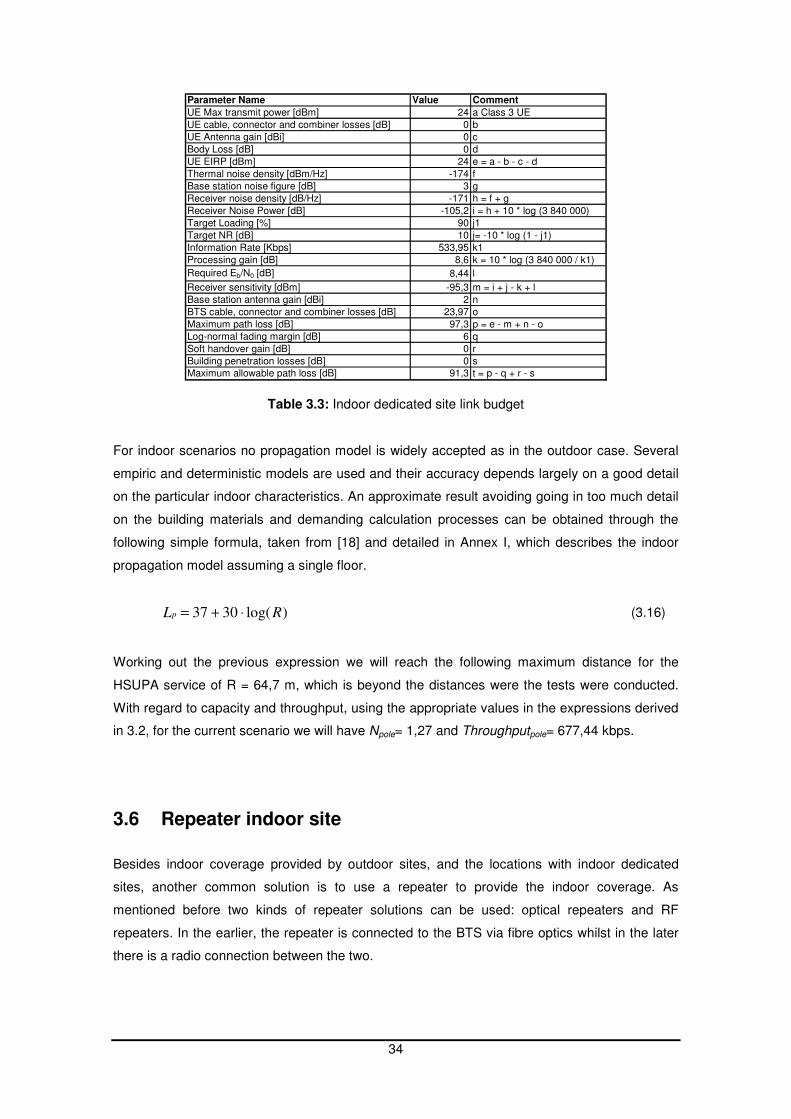
34
Parameter Name Value Comment
UE Max transmit power [dBm] 24 a Class 3 UE
UE cable, connector and combiner losses [dB] 0 b
UE Antenna gain [dBi] 0 c
Body Loss [dB] 0 d
UE EIRP [dBm] 24 e = a - b - c - d
Thermal noise density [dBm/Hz] -174 f
Base station noise figure [dB] 3 g
Receiver noise density [dB/Hz] -171 h = f + g
Receiver Noise Power [dB] -105,2 i = h + 10 * log (3 840 000)
Target Loading [%] 90 j1
Target NR [dB] 10 j= -10 * log (1 - j1)
Information Rate [Kbps] 533,95 k1
Processing gain [dB] 8,6 k = 10 * log (3 840 000 / k1)
Required Eb/N0 [dB] 8,44 l
Receiver sensitivity [dBm] -95,3 m = i + j - k + l
Base station antenna gain [dBi] 2 n
BTS cable, connector and combiner losses [dB] 23,97 o
Maximum path loss [dB] 97,3 p = e - m + n - o
Log-normal fading margin [dB] 6 q
Soft handover gain [dB] 0 r
Building penetration losses [dB] 0 s
Maximum allowable path loss [dB] 91,3 t = p - q + r - s
Table 3.3: Indoor dedicated site link budget
For indoor scenarios no propagation model is widely accepted as in the outdoor case. Several
empiric and deterministic models are used and their accuracy depends largely on a good detail
on the particular indoor characteristics. An approximate result avoiding going in too much detail
on the building materials and demanding calculation processes can be obtained through the
following simple formula, taken from [18] and detailed in Annex I, which describes the indoor
propagation model assuming a single floor.
)log(3037 RLp ⋅+= (3.16)
Working out the previous expression we will reach the following maximum distance for the
HSUPA service of R = 64,7 m, which is beyond the distances were the tests were conducted.
With regard to capacity and throughput, using the appropriate values in the expressions derived
in 3.2, for the current scenario we will have Npole= 1,27 and Throughputpole= 677,44 kbps.
3.6 Repeater indoor site
Besides indoor coverage provided by outdoor sites, and the locations with indoor dedicated
sites, another common solution is to use a repeater to provide the indoor coverage. As
mentioned before two kinds of repeater solutions can be used: optical repeaters and RF
repeaters. In the earlier, the repeater is connected to the BTS via fibre optics whilst in the later
there is a radio connection between the two.
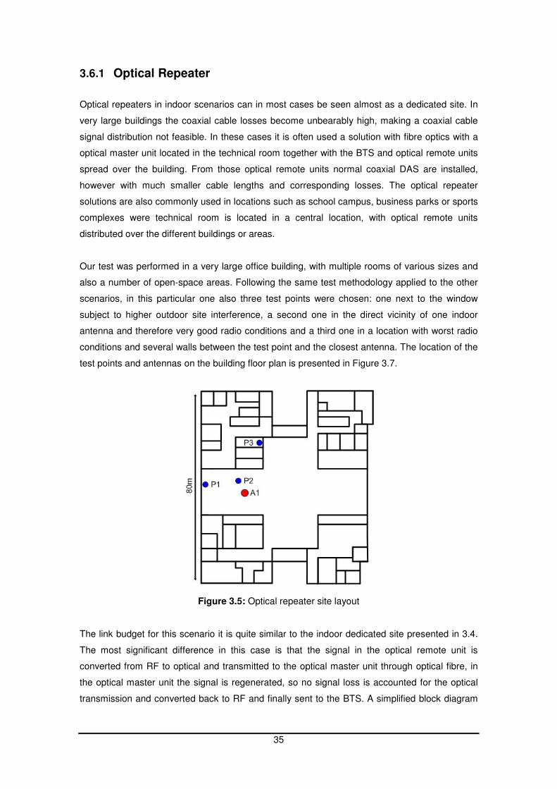
35
3.6.1 Optical Repeater
Optical repeaters in indoor scenarios can in most cases be seen almost as a dedicated site. In
very large buildings the coaxial cable losses become unbearably high, making a coaxial cable
signal distribution not feasible. In these cases it is often used a solution with fibre optics with a
optical master unit located in the technical room together with the BTS and optical remote units
spread over the building. From those optical remote units normal coaxial DAS are installed,
however with much smaller cable lengths and corresponding losses. The optical repeater
solutions are also commonly used in locations such as school campus, business parks or sports
complexes were technical room is located in a central location, with optical remote units
distributed over the different buildings or areas.
Our test was performed in a very large office building, with multiple rooms of various sizes and
also a number of open-space areas. Following the same test methodology applied to the other
scenarios, in this particular one also three test points were chosen: one next to the window
subject to higher outdoor site interference, a second one in the direct vicinity of one indoor
antenna and therefore very good radio conditions and a third one in a location with worst radio
conditions and several walls between the test point and the closest antenna. The location of the
test points and antennas on the building floor plan is presented in Figure 3.7.
Figure 3.5: Optical repeater site layout
The link budget for this scenario it is quite similar to the indoor dedicated site presented in 3.4.
The most significant difference in this case is that the signal in the optical remote unit is
converted from RF to optical and transmitted to the optical master unit through optical fibre, in
the optical master unit the signal is regenerated, so no signal loss is accounted for the optical
transmission and converted back to RF and finally sent to the BTS. A simplified block diagram
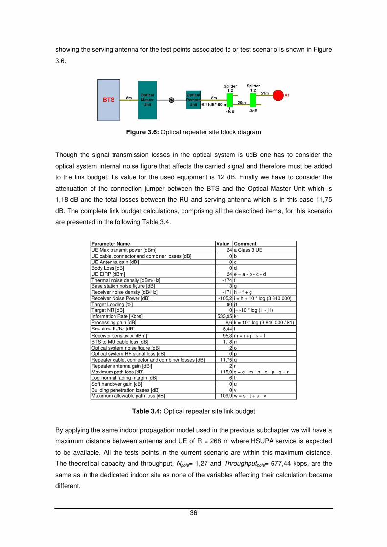
36
showing the serving antenna for the test points associated to or test scenario is shown in Figure
3.6.
Figure 3.6: Optical repeater site block diagram
Though the signal transmission losses in the optical system is 0dB one has to consider the
optical system internal noise figure that affects the carried signal and therefore must be added
to the link budget. Its value for the used equipment is 12 dB. Finally we have to consider the
attenuation of the connection jumper between the BTS and the Optical Master Unit which is
1,18 dB and the total losses between the RU and serving antenna which is in this case 11,75
dB. The complete link budget calculations, comprising all the described items, for this scenario
are presented in the following Table 3.4.
Parameter Name Value Comment
UE Max transmit power [dBm] 24 a Class 3 UE
UE cable, connector and combiner losses [dB] 0 b
UE Antenna gain [dBi] 0 c
Body Loss [dB] 0 d
UE EIRP [dBm] 24 e = a - b - c - d
Thermal noise density [dBm/Hz] -174 f
Base station noise figure [dB] 3 g
Receiver noise density [dB/Hz] -171 h = f + g
Receiver Noise Power [dB] -105,2 i = h + 10 * log (3 840 000)
Target Loading [%] 90 j1
Target NR [dB] 10 j= -10 * log (1 - j1)
Information Rate [Kbps] 533,95 k1
Processing gain [dB] 8,6 k = 10 * log (3 840 000 / k1)
Required Eb/N0 [dB] 8,44 l
Receiver sensitivity [dBm] -95,3 m = i + j - k + l
BTS to MU cable loss [dB] 1,18 n
Optical system noise figure [dB] 12 o
Optical system RF signal loss [dB] 0 p
Repeater cable, connector and combiner losses [dB] 11,75 q
Repeater antenna gain [dBi] 2 r
Maximum path loss [dB] 115,9 s = e - m - n - o - p - q + r
Log-normal fading margin [dB] 6 t
Soft handover gain [dB] 0 u
Building penetration losses [dB] 0 v
Maximum allowable path loss [dB] 109,9 w = s - t + u - v
Table 3.4: Optical repeater site link budget
By applying the same indoor propagation model used in the previous subchapter we will have a
maximum distance between antenna and UE of R = 268 m where HSUPA service is expected
to be available. All the tests points in the current scenario are within this maximum distance.
The theoretical capacity and throughput, Npole= 1,27 and Throughputpole= 677,44 kbps, are the
same as in the dedicated indoor site as none of the variables affecting their calculation became
different.
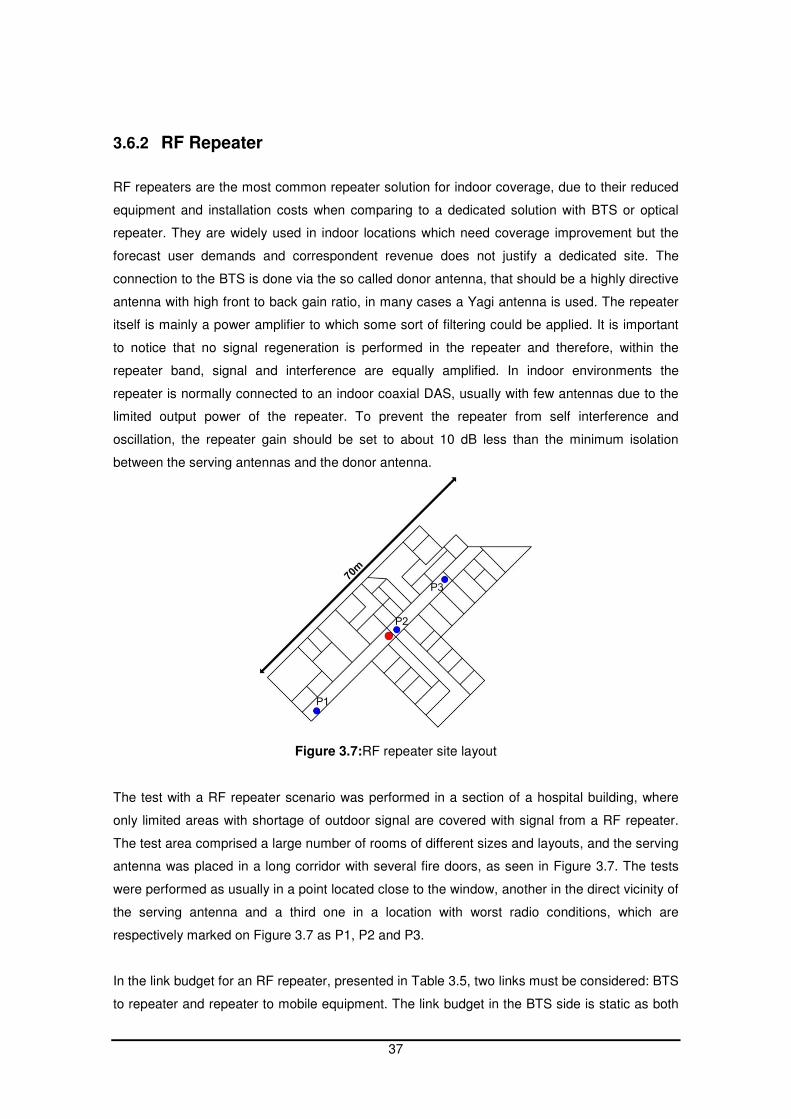
37
3.6.2 RF Repeater
RF repeaters are the most common repeater solution for indoor coverage, due to their reduced
equipment and installation costs when comparing to a dedicated solution with BTS or optical
repeater. They are widely used in indoor locations which need coverage improvement but the
forecast user demands and correspondent revenue does not justify a dedicated site. The
connection to the BTS is done via the so called donor antenna, that should be a highly directive
antenna with high front to back gain ratio, in many cases a Yagi antenna is used. The repeater
itself is mainly a power amplifier to which some sort of filtering could be applied. It is important
to notice that no signal regeneration is performed in the repeater and therefore, within the
repeater band, signal and interference are equally amplified. In indoor environments the
repeater is normally connected to an indoor coaxial DAS, usually with few antennas due to the
limited output power of the repeater. To prevent the repeater from self interference and
oscillation, the repeater gain should be set to about 10 dB less than the minimum isolation
between the serving antennas and the donor antenna.
Figure 3.7:RF repeater site layout
The test with a RF repeater scenario was performed in a section of a hospital building, where
only limited areas with shortage of outdoor signal are covered with signal from a RF repeater.
The test area comprised a large number of rooms of different sizes and layouts, and the serving
antenna was placed in a long corridor with several fire doors, as seen in Figure 3.7. The tests
were performed as usually in a point located close to the window, another in the direct vicinity of
the serving antenna and a third one in a location with worst radio conditions, which are
respectively marked on Figure 3.7 as P1, P2 and P3.
In the link budget for an RF repeater, presented in Table 3.5, two links must be considered: BTS
to repeater and repeater to mobile equipment. The link budget in the BTS side is static as both
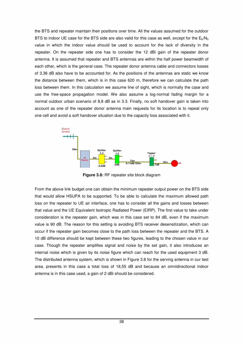
38
the BTS and repeater maintain their positions over time. All the values assumed for the outdoor
BTS to indoor UE case for the BTS side are also valid for this case as well, except for the Eb/N0
value in which the indoor value should be used to account for the lack of diversity in the
repeater. On the repeater side one has to consider the 12 dBi gain of the repeater donor
antenna. It is assumed that repeater and BTS antennas are within the half power beamwidth of
each other, which is the general case. The repeater donor antenna cable and connectors losses
of 3,36 dB also have to be accounted for. As the positions of the antennas are static we know
the distance between them, which is in this case 620 m, therefore we can calculate the path
loss between them. In this calculation we assume line of sight, which is normally the case and
use the free-space propagation model. We also assume a log-normal fading margin for a
normal outdoor urban scenario of 8,8 dB as in 3.3. Finally, no soft handover gain is taken into
account as one of the repeater donor antenna main requests for its location is to repeat only
one cell and avoid a soft handover situation due to the capacity loss associated with it.
Figure 3.8: RF repeater site block diagram
From the above link budget one can obtain the minimum repeater output power on the BTS side
that would allow HSUPA to be supported. To be able to calculate the maximum allowed path
loss on the repeater to UE air interface, one has to consider all the gains and losses between
that value and the UE Equivalent Isotropic Radiated Power (EIRP). The first value to take under
consideration is the repeater gain, which was in this case set to 84 dB, even if the maximum
value is 90 dB. The reason for this setting is avoiding BTS receiver desensitization, which can
occur if the repeater gain becomes close to the path loss between the repeater and the BTS. A
10 dB difference should be kept between these two figures, leading to the chosen value in our
case. Though the repeater amplifies signal and noise by the set gain, it also introduces an
internal noise which is given by its noise figure which can reach for the used equipment 3 dB.
The distributed antenna system, which is shown in Figure 3.8 for the serving antenna in our test
area, presents in this case a total loss of 18,55 dB and because an omnidirectional indoor
antenna is in this case used, a gain of 2 dBi should be considered.
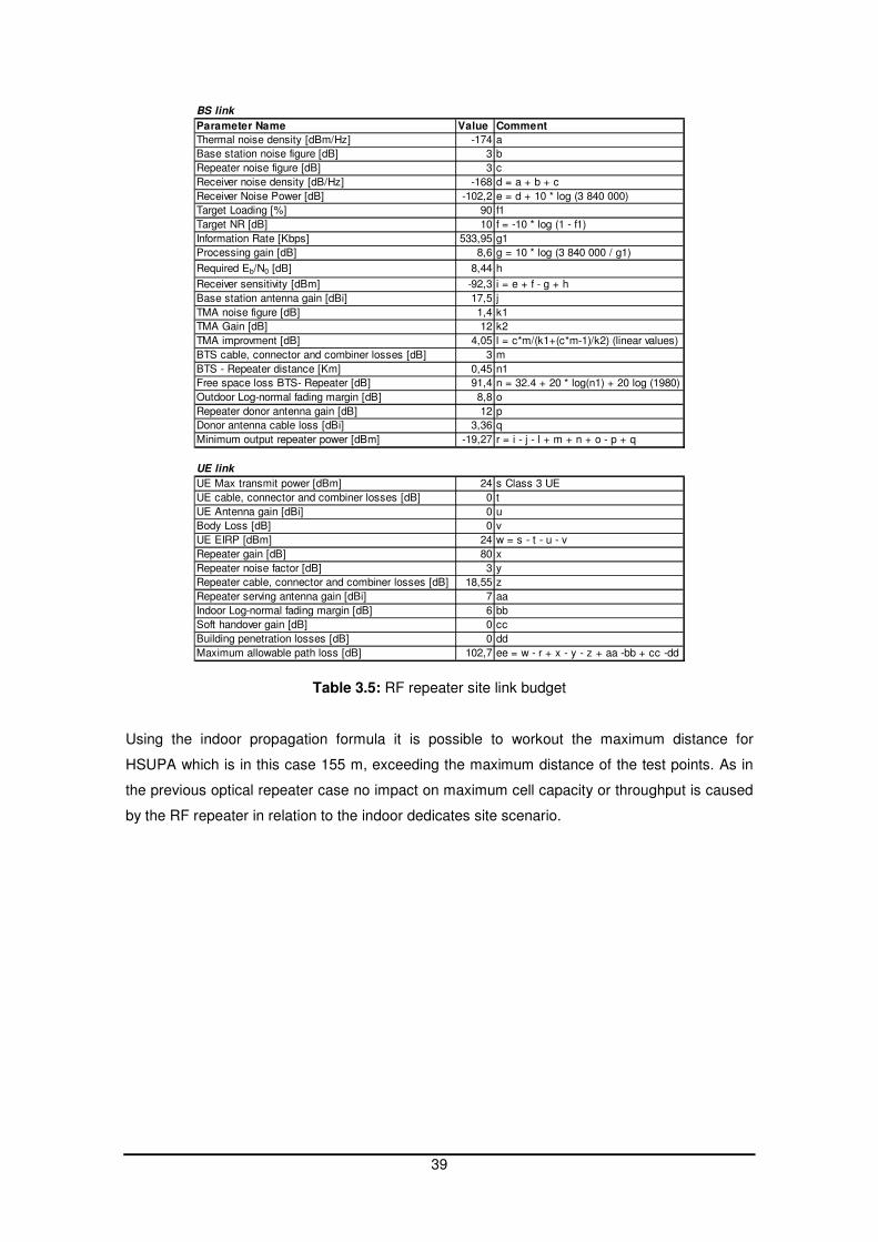
39
BS link
Parameter Name Value Comment
Thermal noise density [dBm/Hz] -174 a
Base station noise figure [dB] 3 b
Repeater noise figure [dB] 3 c
Receiver noise density [dB/Hz] -168 d = a + b + c
Receiver Noise Power [dB] -102,2 e = d + 10 * log (3 840 000)
Target Loading [%] 90 f1
Target NR [dB] 10 f = -10 * log (1 - f1)
Information Rate [Kbps] 533,95 g1
Processing gain [dB] 8,6 g = 10 * log (3 840 000 / g1)
Required Eb/N0 [dB] 8,44 h
Receiver sensitivity [dBm] -92,3 i = e + f - g + h
Base station antenna gain [dBi] 17,5 j
TMA noise figure [dB] 1,4 k1
TMA Gain [dB] 12 k2
TMA improvment [dB] 4,05 l = c*m/(k1+(c*m-1)/k2) (linear values)
BTS cable, connector and combiner losses [dB] 3 m
BTS - Repeater distance [Km] 0,45 n1
Free space loss BTS- Repeater [dB] 91,4 n = 32.4 + 20 * log(n1) + 20 log (1980)
Outdoor Log-normal fading margin [dB] 8,8 o
Repeater donor antenna gain [dB] 12 p
Donor antenna cable loss [dBi] 3,36 q
Minimum output repeater power [dBm] -19,27 r = i - j - l + m + n + o - p + q
UE link
UE Max transmit power [dBm] 24 s Class 3 UE
UE cable, connector and combiner losses [dB] 0 t
UE Antenna gain [dBi] 0 u
Body Loss [dB] 0 v
UE EIRP [dBm] 24 w = s - t - u - v
Repeater gain [dB] 80 x
Repeater noise factor [dB] 3 y
Repeater cable, connector and combiner losses [dB] 18,55 z
Repeater serving antenna gain [dBi] 7 aa
Indoor Log-normal fading margin [dB] 6 bb
Soft handover gain [dB] 0 cc
Building penetration losses [dB] 0 dd
Maximum allowable path loss [dB] 102,7 ee = w - r + x - y - z + aa -bb + cc -dd
Table 3.5: RF repeater site link budget
Using the indoor propagation formula it is possible to workout the maximum distance for
HSUPA which is in this case 155 m, exceeding the maximum distance of the test points. As in
the previous optical repeater case no impact on maximum cell capacity or throughput is caused
by the RF repeater in relation to the indoor dedicates site scenario.

40

41
4 Test Results
This chapter presents the main results of the tests conducted in the several considered
scenarios. First, the results of the individual scenarios are shown, and afterwards a comparison
between the results in different scenarios is presented.
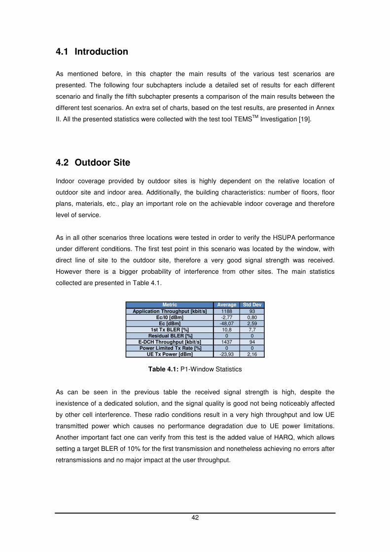
42
4.1 Introduction
As mentioned before, in this chapter the main results of the various test scenarios are
presented. The following four subchapters include a detailed set of results for each different
scenario and finally the fifth subchapter presents a comparison of the main results between the
different test scenarios. An extra set of charts, based on the test results, are presented in Annex
II. All the presented statistics were collected with the test tool TEMSTM
Investigation [19].
4.2 Outdoor Site Indoor coverage provided by outdoor sites is highly dependent on the relative location of
outdoor site and indoor area. Additionally, the building characteristics: number of floors, floor
plans, materials, etc., play an important role on the achievable indoor coverage and therefore
level of service.
As in all other scenarios three locations were tested in order to verify the HSUPA performance
under different conditions. The first test point in this scenario was located by the window, with
direct line of site to the outdoor site, therefore a very good signal strength was received.
However there is a bigger probability of interference from other sites. The main statistics
collected are presented in Table 4.1.
Metric Average Std Dev
Application Throughput [kbit/s] 1188 93
Ec/I0 [dBm] -2,77 0,80
Ec [dBm] -48,07 2,59
1st Tx BLER [%] 10,8 7,7
Residual BLER [%] 0 0
E-DCH Throughput [kbit/s] 1437 94
Power Limited Tx Rate [%] 0 0
UE Tx Power [dBm] -23,93 2,16
Table 4.1: P1-Window Statistics
As can be seen in the previous table the received signal strength is high, despite the
inexistence of a dedicated solution, and the signal quality is good not being noticeably affected
by other cell interference. These radio conditions result in a very high throughput and low UE
transmitted power which causes no performance degradation due to UE power limitations.
Another important fact one can verify from this test is the added value of HARQ, which allows
setting a target BLER of 10% for the first transmission and nonetheless achieving no errors after
retransmissions and no major impact at the user throughput.
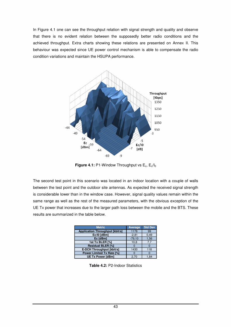
43
In Figure 4.1 one can see the throughput relation with signal strength and quality and observe
that there is no evident relation between the supposedly better radio conditions and the
achieved throughput. Extra charts showing these relations are presented on Annex II. This
behaviour was expected since UE power control mechanism is able to compensate the radio
condition variations and maintain the HSUPA performance.
Figure 4.1: P1-Window Throughput vs Ec, Ec/I0
The second test point in this scenario was located in an indoor location with a couple of walls
between the test point and the outdoor site antennas. As expected the received signal strength
is considerable lower than in the window case. However, signal quality values remain within the
same range as well as the rest of the measured parameters, with the obvious exception of the
UE Tx power that increases due to the larger path loss between the mobile and the BTS. These
results are summarized in the table below.
Metric Average Std Dev
Application Throughput [kbit/s] 1178 99
Ec/I0 [dBm] -2,81 0,49
Ec [dBm] -79,10 1,56
1st Tx BLER [%] 10,8 7,7
Residual BLER [%] 0 0
E-DCH Throughput [kbit/s] 1430 118
Power Limited Tx Rate [%] 0 0
UE Tx Power [dBm] 2,70 1,84
Table 4.2: P2-Indoor Statistics
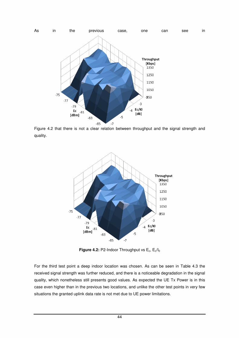
44
As in the previous case, one can see in
Figure 4.2 that there is not a clear relation between throughput and the signal strength and
quality.
Figure 4.2: P2-Indoor Throughput vs Ec, Ec/I0
For the third test point a deep indoor location was chosen. As can be seen in Table 4.3 the
received signal strength was further reduced, and there is a noticeable degradation in the signal
quality, which nonetheless still presents good values. As expected the UE Tx Power is in this
case even higher than in the previous two locations, and unlike the other test points in very few
situations the granted uplink data rate is not met due to UE power limitations.
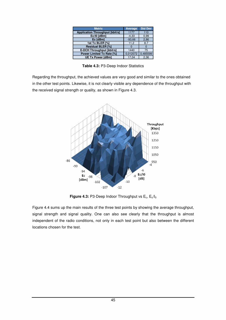
45
Metric Average Std Dev
Application Throughput [kbit/s] 1177 110
Ec/I0 [dBm] -4,33 0,99
Ec [dBm] -93,66 2,86
1st Tx BLER [%] 11,2 8,7
Residual BLER [%] 0 0
E-DCH Throughput [kbit/s] 1440 75
Power Limited Tx Rate [%] 0,012072 0,485599
UE Tx Power [dBm] 17,04 2,36
Table 4.3: P3-Deep Indoor Statistics
Regarding the throughput, the achieved values are very good and similar to the ones obtained
in the other test points. Likewise, it is not clearly visible any dependence of the throughput with
the received signal strength or quality, as shown in Figure 4.3.
Figure 4.3: P3-Deep Indoor Throughput vs Ec, Ec/I0
Figure 4.4 sums up the main results of the three test points by showing the average throughput,
signal strength and signal quality. One can also see clearly that the throughput is almost
independent of the radio conditions, not only in each test point but also between the different
locations chosen for the test.
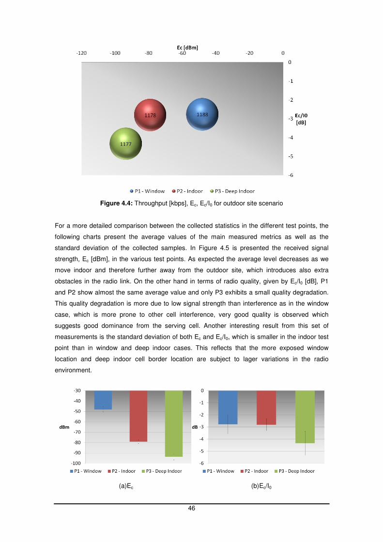
46
Figure 4.4: Throughput [kbps], Ec, Ec/I0 for outdoor site scenario
For a more detailed comparison between the collected statistics in the different test points, the
following charts present the average values of the main measured metrics as well as the
standard deviation of the collected samples. In Figure 4.5 is presented the received signal
strength, Ec [dBm], in the various test points. As expected the average level decreases as we
move indoor and therefore further away from the outdoor site, which introduces also extra
obstacles in the radio link. On the other hand in terms of radio quality, given by Ec/I0 [dB], P1
and P2 show almost the same average value and only P3 exhibits a small quality degradation.
This quality degradation is more due to low signal strength than interference as in the window
case, which is more prone to other cell interference, very good quality is observed which
suggests good dominance from the serving cell. Another interesting result from this set of
measurements is the standard deviation of both Ec and Ec/I0, which is smaller in the indoor test
point than in window and deep indoor cases. This reflects that the more exposed window
location and deep indoor cell border location are subject to lager variations in the radio
environment.
(a)Ec (b)Ec/I0
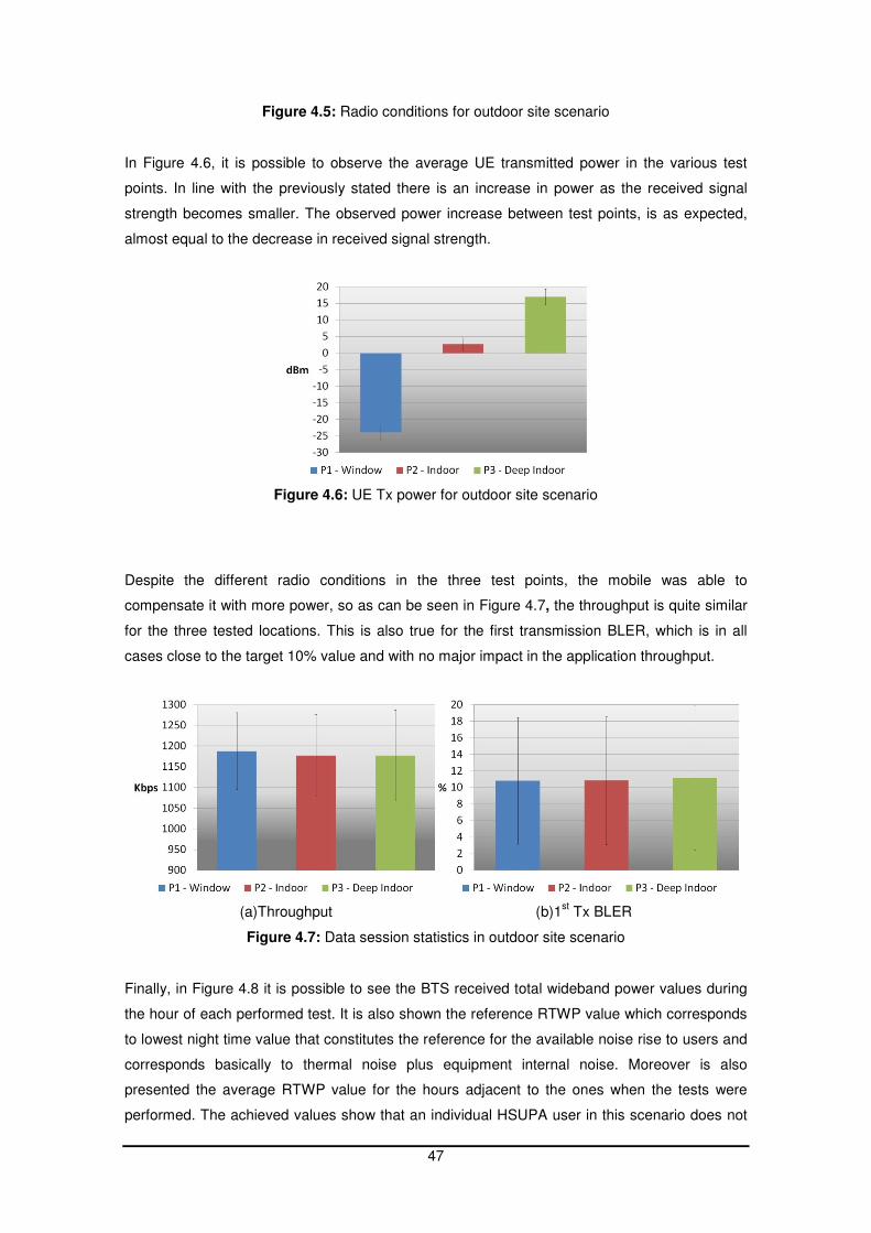
47
Figure 4.5: Radio conditions for outdoor site scenario
In Figure 4.6, it is possible to observe the average UE transmitted power in the various test
points. In line with the previously stated there is an increase in power as the received signal
strength becomes smaller. The observed power increase between test points, is as expected,
almost equal to the decrease in received signal strength.
Figure 4.6: UE Tx power for outdoor site scenario
Despite the different radio conditions in the three test points, the mobile was able to
compensate it with more power, so as can be seen in Figure 4.7, the throughput is quite similar
for the three tested locations. This is also true for the first transmission BLER, which is in all
cases close to the target 10% value and with no major impact in the application throughput.
(a)Throughput (b)1st Tx BLER
Figure 4.7: Data session statistics in outdoor site scenario
Finally, in Figure 4.8 it is possible to see the BTS received total wideband power values during
the hour of each performed test. It is also shown the reference RTWP value which corresponds
to lowest night time value that constitutes the reference for the available noise rise to users and
corresponds basically to thermal noise plus equipment internal noise. Moreover is also
presented the average RTWP value for the hours adjacent to the ones when the tests were
performed. The achieved values show that an individual HSUPA user in this scenario does not
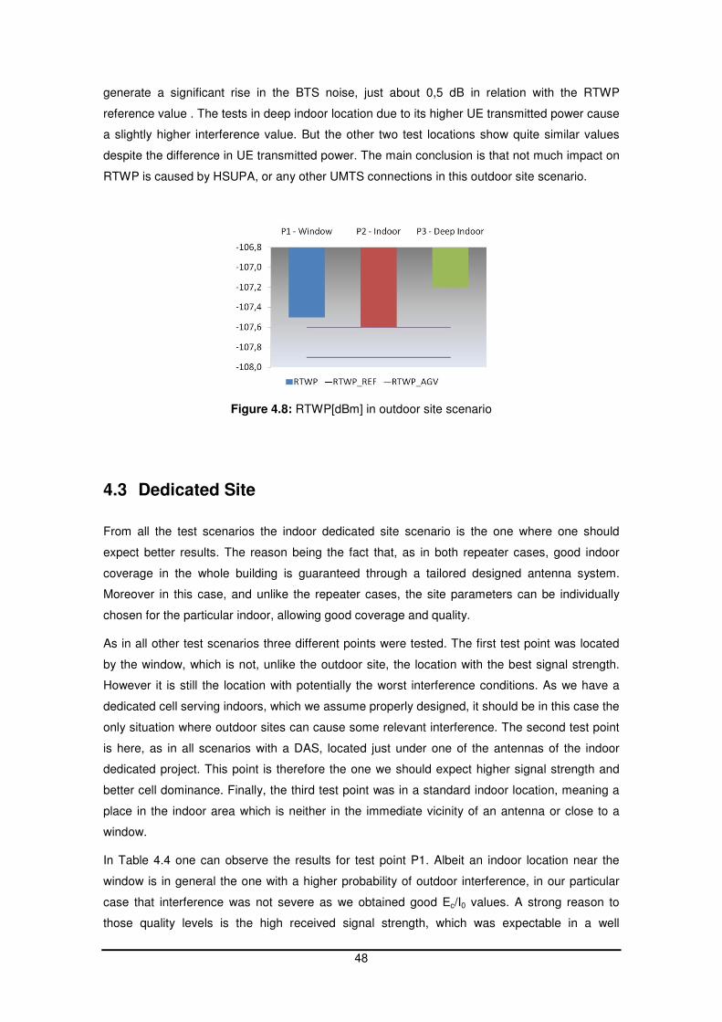
48
generate a significant rise in the BTS noise, just about 0,5 dB in relation with the RTWP
reference value . The tests in deep indoor location due to its higher UE transmitted power cause
a slightly higher interference value. But the other two test locations show quite similar values
despite the difference in UE transmitted power. The main conclusion is that not much impact on
RTWP is caused by HSUPA, or any other UMTS connections in this outdoor site scenario.
Figure 4.8: RTWP[dBm] in outdoor site scenario
4.3 Dedicated Site
From all the test scenarios the indoor dedicated site scenario is the one where one should
expect better results. The reason being the fact that, as in both repeater cases, good indoor
coverage in the whole building is guaranteed through a tailored designed antenna system.
Moreover in this case, and unlike the repeater cases, the site parameters can be individually
chosen for the particular indoor, allowing good coverage and quality.
As in all other test scenarios three different points were tested. The first test point was located
by the window, which is not, unlike the outdoor site, the location with the best signal strength.
However it is still the location with potentially the worst interference conditions. As we have a
dedicated cell serving indoors, which we assume properly designed, it should be in this case the
only situation where outdoor sites can cause some relevant interference. The second test point
is here, as in all scenarios with a DAS, located just under one of the antennas of the indoor
dedicated project. This point is therefore the one we should expect higher signal strength and
better cell dominance. Finally, the third test point was in a standard indoor location, meaning a
place in the indoor area which is neither in the immediate vicinity of an antenna or close to a
window.
In Table 4.4 one can observe the results for test point P1. Albeit an indoor location near the
window is in general the one with a higher probability of outdoor interference, in our particular
case that interference was not severe as we obtained good Ec/I0 values. A strong reason to
those quality levels is the high received signal strength, which was expectable in a well
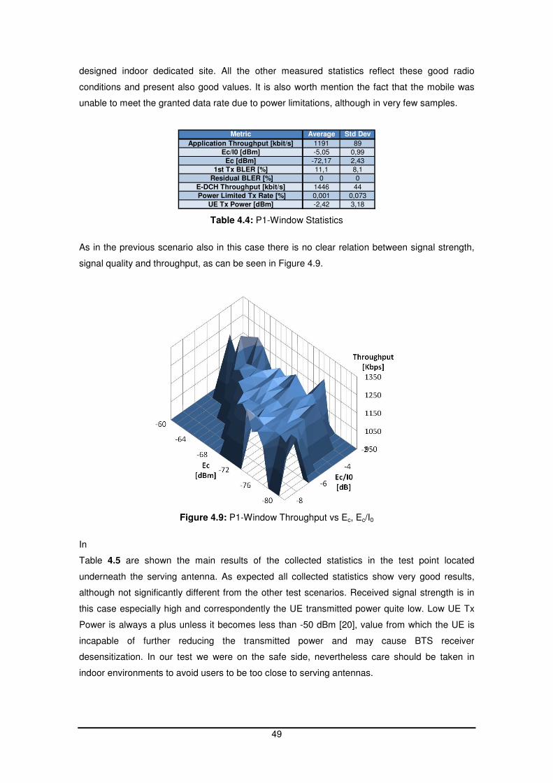
49
designed indoor dedicated site. All the other measured statistics reflect these good radio
conditions and present also good values. It is also worth mention the fact that the mobile was
unable to meet the granted data rate due to power limitations, although in very few samples.
Metric Average Std Dev
Application Throughput [kbit/s] 1191 89
Ec/I0 [dBm] -5,05 0,99
Ec [dBm] -72,17 2,43
1st Tx BLER [%] 11,1 8,1
Residual BLER [%] 0 0
E-DCH Throughput [kbit/s] 1446 44
Power Limited Tx Rate [%] 0,001 0,073
UE Tx Power [dBm] -2,42 3,18
Table 4.4: P1-Window Statistics
As in the previous scenario also in this case there is no clear relation between signal strength,
signal quality and throughput, as can be seen in Figure 4.9.
Figure 4.9: P1-Window Throughput vs Ec, Ec/I0
In
Table 4.5 are shown the main results of the collected statistics in the test point located
underneath the serving antenna. As expected all collected statistics show very good results,
although not significantly different from the other test scenarios. Received signal strength is in
this case especially high and correspondently the UE transmitted power quite low. Low UE Tx
Power is always a plus unless it becomes less than -50 dBm [20], value from which the UE is
incapable of further reducing the transmitted power and may cause BTS receiver
desensitization. In our test we were on the safe side, nevertheless care should be taken in
indoor environments to avoid users to be too close to serving antennas.
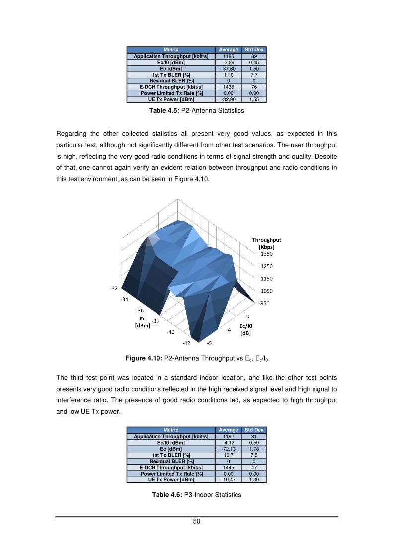
50
Metric Average Std Dev
Application Throughput [kbit/s] 1185 89
Ec/I0 [dBm] -2,89 0,45
Ec [dBm] -37,60 1,50
1st Tx BLER [%] 11,0 7,7
Residual BLER [%] 0 0
E-DCH Throughput [kbit/s] 1438 76
Power Limited Tx Rate [%] 0,00 0,00
UE Tx Power [dBm] -32,90 1,55
Table 4.5: P2-Antenna Statistics
Regarding the other collected statistics all present very good values, as expected in this
particular test, although not significantly different from other test scenarios. The user throughput
is high, reflecting the very good radio conditions in terms of signal strength and quality. Despite
of that, one cannot again verify an evident relation between throughput and radio conditions in
this test environment, as can be seen in Figure 4.10.
Figure 4.10: P2-Antenna Throughput vs Ec, Ec/I0
The third test point was located in a standard indoor location, and like the other test points
presents very good radio conditions reflected in the high received signal level and high signal to
interference ratio. The presence of good radio conditions led, as expected to high throughput
and low UE Tx power.
Metric Average Std Dev
Application Throughput [kbit/s] 1192 81
Ec/I0 [dBm] -4,12 0,59
Ec [dBm] -72,13 1,78
1st Tx BLER [%] 10,7 7,5
Residual BLER [%] 0 0
E-DCH Throughput [kbit/s] 1445 47
Power Limited Tx Rate [%] 0,00 0,00
UE Tx Power [dBm] -10,47 1,39
Table 4.6: P3-Indoor Statistics
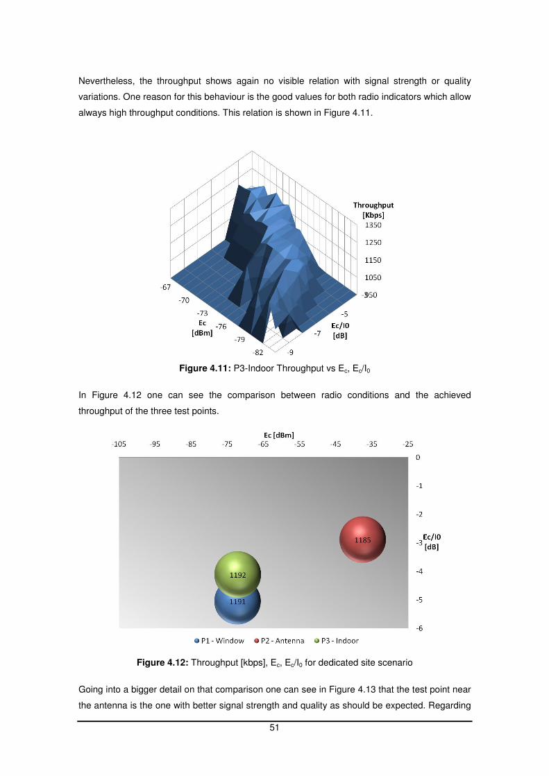
51
Nevertheless, the throughput shows again no visible relation with signal strength or quality
variations. One reason for this behaviour is the good values for both radio indicators which allow
always high throughput conditions. This relation is shown in Figure 4.11.
Figure 4.11: P3-Indoor Throughput vs Ec, Ec/I0
In Figure 4.12 one can see the comparison between radio conditions and the achieved
throughput of the three test points.
Figure 4.12: Throughput [kbps], Ec, Ec/I0 for dedicated site scenario
Going into a bigger detail on that comparison one can see in Figure 4.13 that the test point near
the antenna is the one with better signal strength and quality as should be expected. Regarding

52
the other two test points there is no much difference in terms of received signal strength.
However, regarding the Ec/I0 values, despite of being both good, there is a noticeable difference
between the worse window test point result and the better standard indoor test point result. This
was expected due to the bigger exposition of P1 to the outdoor interferers. The standard
deviation of the values is also bigger in the window case which is characteristic of a more
dynamic radio environment in contrast to a more static radio environment existent in P3, and
even more in P2.
(a)Ec (b)Ec/I0
Figure 4.13: Radio conditions for dedicated site scenario
As a result of the previously stated regarding the good radio conditions, the average UE
transmitted power, shown in Figure 4.14, is well below its maximum limit for all the test points. In
line with what was observed with the radio quality it is possible to see that in the window test
point the UE transmitted power it is in average higher than in the indoor test point, despite of the
received signal strength being almost the same. In the window case the UE has to raise its
transmitted power in order to cope with the higher external interference.
Figure 4.14: UE Tx power for dedicated site scenario
Despite the slightly different radio condition experimented by the UE in the three test points, the
UE is able to compensate those variations and still maintain a very good and even throughput in
all cases, as can be seen in Figure 4.15.
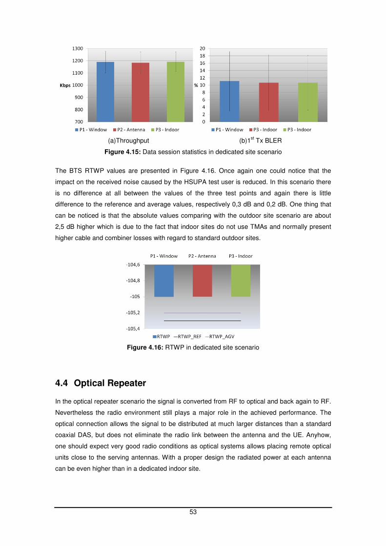
53
(a)Throughput (b)1st Tx BLER
Figure 4.15: Data session statistics in dedicated site scenario
The BTS RTWP values are presented in Figure 4.16. Once again one could notice that the
impact on the received noise caused by the HSUPA test user is reduced. In this scenario there
is no difference at all between the values of the three test points and again there is little
difference to the reference and average values, respectively 0,3 dB and 0,2 dB. One thing that
can be noticed is that the absolute values comparing with the outdoor site scenario are about
2,5 dB higher which is due to the fact that indoor sites do not use TMAs and normally present
higher cable and combiner losses with regard to standard outdoor sites.
Figure 4.16: RTWP in dedicated site scenario
4.4 Optical Repeater In the optical repeater scenario the signal is converted from RF to optical and back again to RF.
Nevertheless the radio environment still plays a major role in the achieved performance. The
optical connection allows the signal to be distributed at much larger distances than a standard
coaxial DAS, but does not eliminate the radio link between the antenna and the UE. Anyhow,
one should expect very good radio conditions as optical systems allows placing remote optical
units close to the serving antennas. With a proper design the radiated power at each antenna
can be even higher than in a dedicated indoor site.
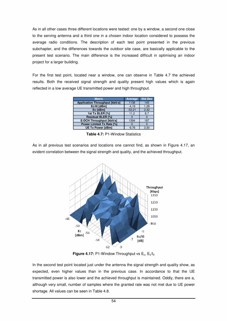
54
As in all other cases three different locations were tested: one by a window, a second one close
to the serving antenna and a third one in a chosen indoor location considered to possess the
average radio conditions. The description of each test point presented in the previous
subchapter, and the differences towards the outdoor site case, are basically applicable to the
present test scenario. The main difference is the increased difficult in optimising an indoor
project for a larger building.
For the first test point, located near a window, one can observe in Table 4.7 the achieved
results. Both the received signal strength and quality present high values which is again
reflected in a low average UE transmitted power and high throughput.
Metric Average Std Dev
Application Throughput [kbit/s] 1138 145
Ec/I0 [dBm] -4,19 1,28
Ec [dBm] -53,21 2,42
1st Tx BLER [%] 11,2 8,7
Residual BLER [%] 0 0
E-DCH Throughput [kbit/s] 1394 187
Power Limited Tx Rate [%] 0 0
UE Tx Power [dBm] -9,76 3,50
Table 4.7: P1-Window Statistics
As in all previous test scenarios and locations one cannot find, as shown in Figure 4.17, an
evident correlation between the signal strength and quality, and the achieved throughput.
Figure 4.17: P1-Window Throughput vs Ec, Ec/I0
In the second test point located just under the antenna the signal strength and quality show, as
expected, even higher values than in the previous case. In accordance to that the UE
transmitted power is also lower and the achieved throughput is maintained. Oddly, there are a,
although very small, number of samples where the granted rate was not met due to UE power
shortage. All values can be seen in Table 4.8.
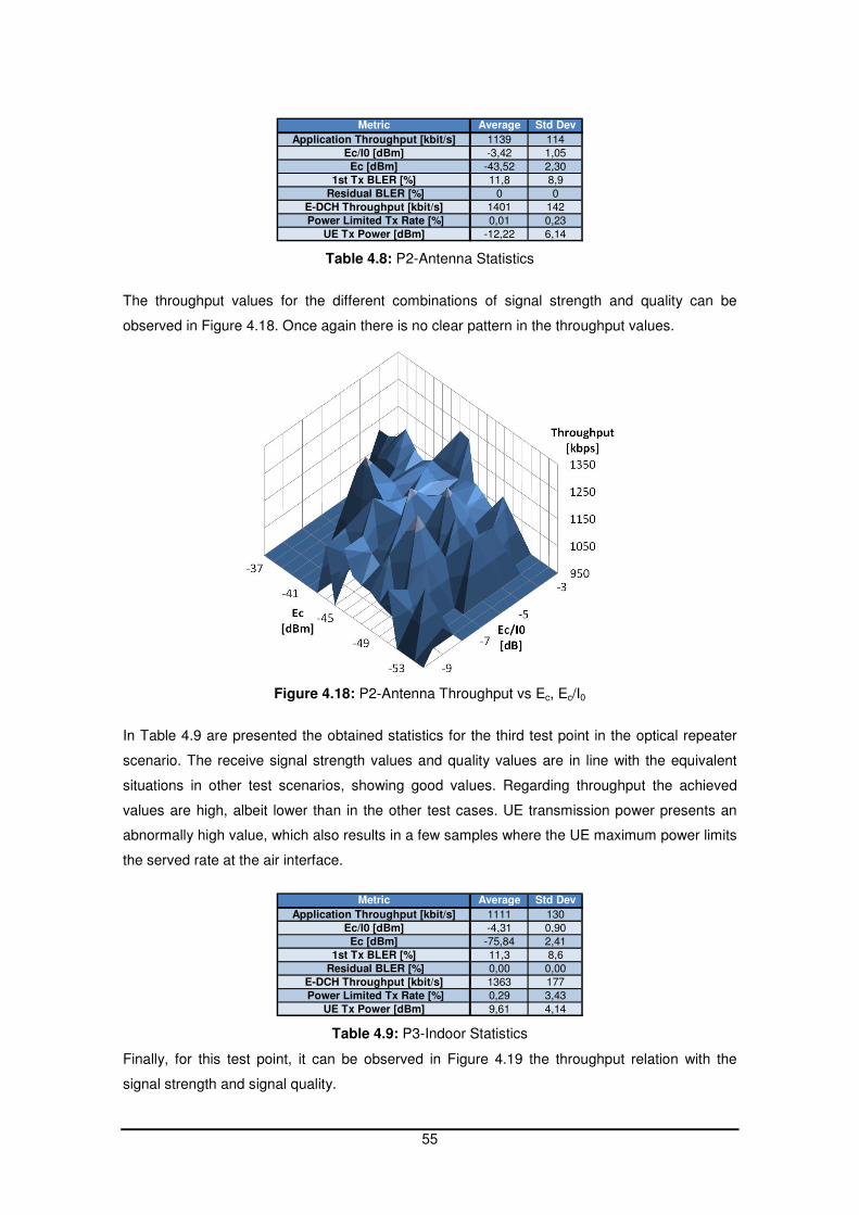
55
Metric Average Std Dev
Application Throughput [kbit/s] 1139 114
Ec/I0 [dBm] -3,42 1,05
Ec [dBm] -43,52 2,30
1st Tx BLER [%] 11,8 8,9
Residual BLER [%] 0 0
E-DCH Throughput [kbit/s] 1401 142
Power Limited Tx Rate [%] 0,01 0,23
UE Tx Power [dBm] -12,22 6,14
Table 4.8: P2-Antenna Statistics
The throughput values for the different combinations of signal strength and quality can be
observed in Figure 4.18. Once again there is no clear pattern in the throughput values.
Figure 4.18: P2-Antenna Throughput vs Ec, Ec/I0
In Table 4.9 are presented the obtained statistics for the third test point in the optical repeater
scenario. The receive signal strength values and quality values are in line with the equivalent
situations in other test scenarios, showing good values. Regarding throughput the achieved
values are high, albeit lower than in the other test cases. UE transmission power presents an
abnormally high value, which also results in a few samples where the UE maximum power limits
the served rate at the air interface.
Metric Average Std Dev
Application Throughput [kbit/s] 1111 130
Ec/I0 [dBm] -4,31 0,90
Ec [dBm] -75,84 2,41
1st Tx BLER [%] 11,3 8,6
Residual BLER [%] 0,00 0,00
E-DCH Throughput [kbit/s] 1363 177
Power Limited Tx Rate [%] 0,29 3,43
UE Tx Power [dBm] 9,61 4,14
Table 4.9: P3-Indoor Statistics
Finally, for this test point, it can be observed in Figure 4.19 the throughput relation with the
signal strength and signal quality.
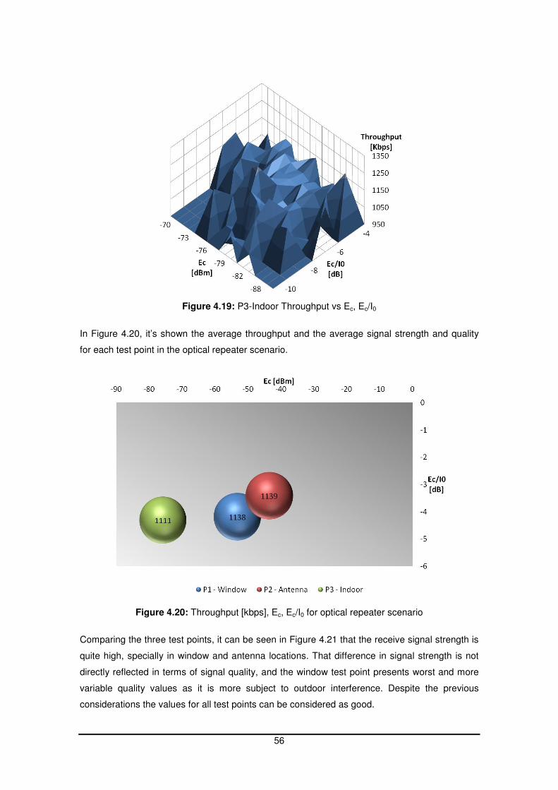
56
Figure 4.19: P3-Indoor Throughput vs Ec, Ec/I0
In Figure 4.20, it’s shown the average throughput and the average signal strength and quality
for each test point in the optical repeater scenario.
Figure 4.20: Throughput [kbps], Ec, Ec/I0 for optical repeater scenario
Comparing the three test points, it can be seen in Figure 4.21 that the receive signal strength is
quite high, specially in window and antenna locations. That difference in signal strength is not
directly reflected in terms of signal quality, and the window test point presents worst and more
variable quality values as it is more subject to outdoor interference. Despite the previous
considerations the values for all test points can be considered as good.
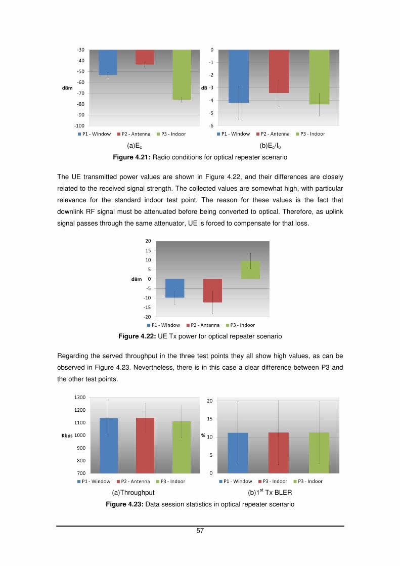
57
(a)Ec (b)Ec/I0
Figure 4.21: Radio conditions for optical repeater scenario
The UE transmitted power values are shown in Figure 4.22, and their differences are closely
related to the received signal strength. The collected values are somewhat high, with particular
relevance for the standard indoor test point. The reason for these values is the fact that
downlink RF signal must be attenuated before being converted to optical. Therefore, as uplink
signal passes through the same attenuator, UE is forced to compensate for that loss.
Figure 4.22: UE Tx power for optical repeater scenario
Regarding the served throughput in the three test points they all show high values, as can be
observed in Figure 4.23. Nevertheless, there is in this case a clear difference between P3 and
the other test points.
(a)Throughput (b)1st Tx BLER
Figure 4.23: Data session statistics in optical repeater scenario
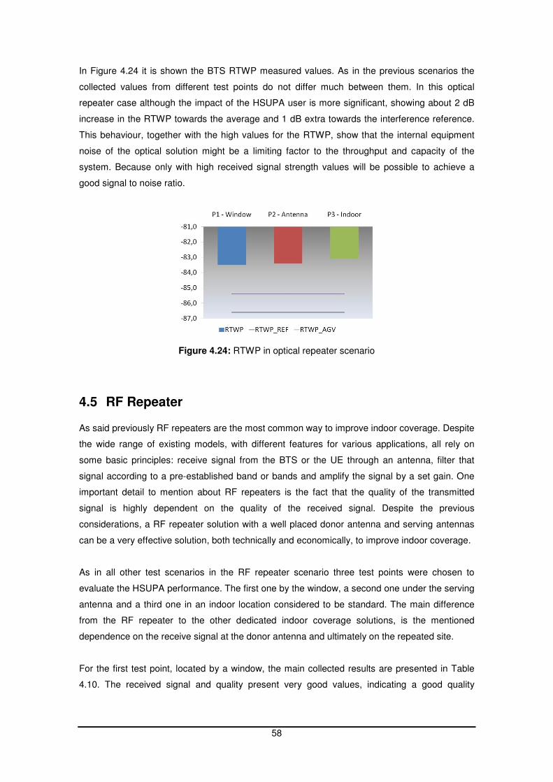
58
In Figure 4.24 it is shown the BTS RTWP measured values. As in the previous scenarios the
collected values from different test points do not differ much between them. In this optical
repeater case although the impact of the HSUPA user is more significant, showing about 2 dB
increase in the RTWP towards the average and 1 dB extra towards the interference reference.
This behaviour, together with the high values for the RTWP, show that the internal equipment
noise of the optical solution might be a limiting factor to the throughput and capacity of the
system. Because only with high received signal strength values will be possible to achieve a
good signal to noise ratio.
Figure 4.24: RTWP in optical repeater scenario
4.5 RF Repeater As said previously RF repeaters are the most common way to improve indoor coverage. Despite
the wide range of existing models, with different features for various applications, all rely on
some basic principles: receive signal from the BTS or the UE through an antenna, filter that
signal according to a pre-established band or bands and amplify the signal by a set gain. One
important detail to mention about RF repeaters is the fact that the quality of the transmitted
signal is highly dependent on the quality of the received signal. Despite the previous
considerations, a RF repeater solution with a well placed donor antenna and serving antennas
can be a very effective solution, both technically and economically, to improve indoor coverage.
As in all other test scenarios in the RF repeater scenario three test points were chosen to
evaluate the HSUPA performance. The first one by the window, a second one under the serving
antenna and a third one in an indoor location considered to be standard. The main difference
from the RF repeater to the other dedicated indoor coverage solutions, is the mentioned
dependence on the receive signal at the donor antenna and ultimately on the repeated site.
For the first test point, located by a window, the main collected results are presented in Table
4.10. The received signal and quality present very good values, indicating a good quality
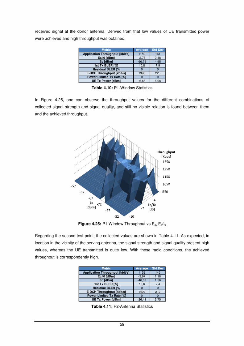
59
received signal at the donor antenna. Derived from that low values of UE transmitted power
were achieved and high throughput was obtained.
Metric Average Std Dev
Application Throughput [kbit/s] 1159 161
Ec/I0 [dBm] -2,76 0,48
Ec [dBm] -66,78 4,95
1st Tx BLER [%] 10,8 7,9
Residual BLER [%] 0 0
E-DCH Throughput [kbit/s] 1398 225
Power Limited Tx Rate [%] 0 0
UE Tx Power [dBm] -6,66 6,08
Table 4.10: P1-Window Statistics
In Figure 4.25, one can observe the throughput values for the different combinations of
collected signal strength and signal quality, and still no visible relation is found between them
and the achieved throughput.
Figure 4.25: P1-Window Throughput vs Ec, Ec/I0
Regarding the second test point, the collected values are shown in Table 4.11. As expected, in
location in the vicinity of the serving antenna, the signal strength and signal quality present high
values, whereas the UE transmitted is quite low. With these radio conditions, the achieved
throughput is correspondently high.
Metric Average Std Dev
Application Throughput [kbit/s] 1159 145
Ec/I0 [dBm] -3,97 1,18
Ec [dBm] -46,03 1,56
1st Tx BLER [%] 10,6 7,4
Residual BLER [%] 0 0
E-DCH Throughput [kbit/s] 1409 212
Power Limited Tx Rate [%] 0 0
UE Tx Power [dBm] -26,41 3,75
Table 4.11: P2-Antenna Statistics

60
In Figure 4.26, it can be seen the average throughput values for the different signal strength and
signal quality values and once again there is no direct relation between the radio conditions and
the throughput.
Figure 4.26: P2-Antenna Throughput vs Ec, Ec/I0
Finally the results for the third test point are presented in Table 4.12. The achieved results are
noticeable lower in terms of signal strength, although maintaining an acceptable value as should
be expected in a location with a dedicated coverage solution. The Ec/I0 values remain quite high
whereas the UE transmitted power shows somewhat higher values. As a result of the previously
stated the achieved HSUPA throughput is also for this test point close to the theoretical limit.
Metric Average Std Dev
Application Throughput [kbit/s] 1153 167
Ec/I0 [dBm] -4,96 1,20
Ec [dBm] -81,05 5,16
1st Tx BLER [%] 10,7 8,2
Residual BLER [%] 0 0
E-DCH Throughput [kbit/s] 1402 227
Power Limited Tx Rate [%] 0 0
UE Tx Power [dBm] 2,73 4,28
Table 4.12: P3-Indoor Statistics
In Figure 4.27, the relation between throughput and radio conditions are presented. As in all test
points there is no clear relation between those two factors.
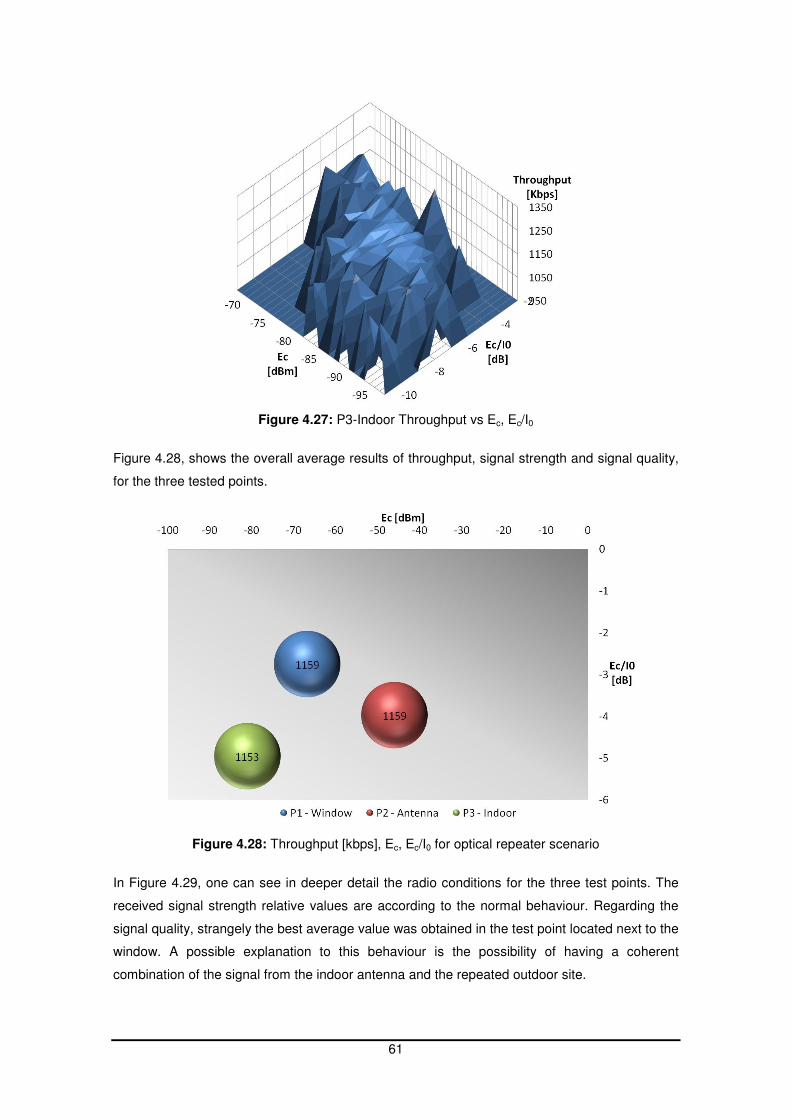
61
Figure 4.27: P3-Indoor Throughput vs Ec, Ec/I0
Figure 4.28, shows the overall average results of throughput, signal strength and signal quality,
for the three tested points.
Figure 4.28: Throughput [kbps], Ec, Ec/I0 for optical repeater scenario
In Figure 4.29, one can see in deeper detail the radio conditions for the three test points. The
received signal strength relative values are according to the normal behaviour. Regarding the
signal quality, strangely the best average value was obtained in the test point located next to the
window. A possible explanation to this behaviour is the possibility of having a coherent
combination of the signal from the indoor antenna and the repeated outdoor site.
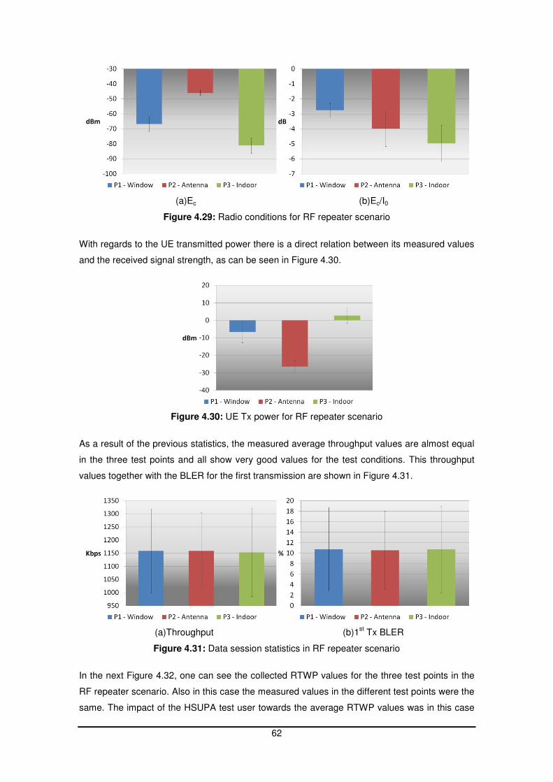
62
(a)Ec (b)Ec/I0
Figure 4.29: Radio conditions for RF repeater scenario
With regards to the UE transmitted power there is a direct relation between its measured values
and the received signal strength, as can be seen in Figure 4.30.
Figure 4.30: UE Tx power for RF repeater scenario
As a result of the previous statistics, the measured average throughput values are almost equal
in the three test points and all show very good values for the test conditions. This throughput
values together with the BLER for the first transmission are shown in Figure 4.31.
(a)Throughput (b)1st Tx BLER
Figure 4.31: Data session statistics in RF repeater scenario
In the next Figure 4.32, one can see the collected RTWP values for the three test points in the
RF repeater scenario. Also in this case the measured values in the different test points were the
same. The impact of the HSUPA test user towards the average RTWP values was in this case
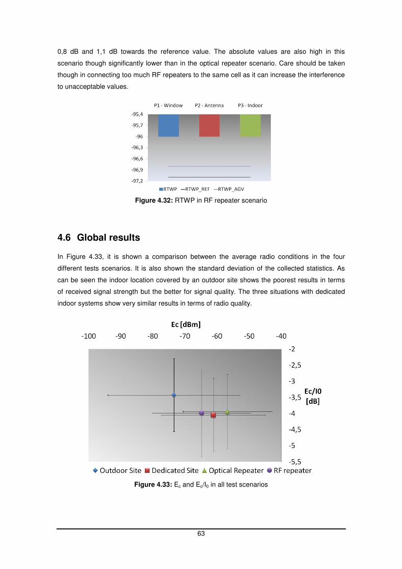
63
0,8 dB and 1,1 dB towards the reference value. The absolute values are also high in this
scenario though significantly lower than in the optical repeater scenario. Care should be taken
though in connecting too much RF repeaters to the same cell as it can increase the interference
to unacceptable values.
Figure 4.32: RTWP in RF repeater scenario
4.6 Global results In Figure 4.33, it is shown a comparison between the average radio conditions in the four
different tests scenarios. It is also shown the standard deviation of the collected statistics. As
can be seen the indoor location covered by an outdoor site shows the poorest results in terms
of received signal strength but the better for signal quality. The three situations with dedicated
indoor systems show very similar results in terms of radio quality.
Figure 4.33: Ec and Ec/I0 in all test scenarios
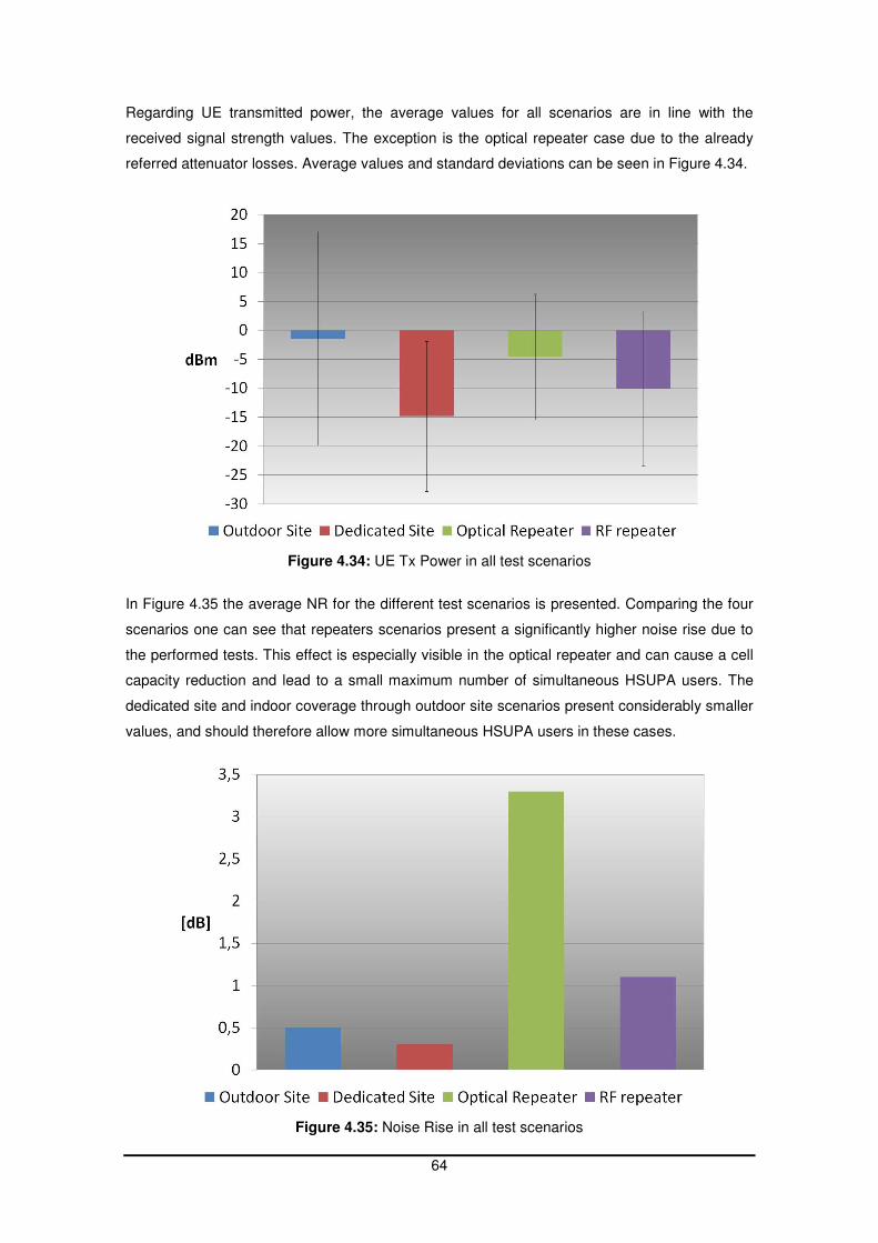
64
Regarding UE transmitted power, the average values for all scenarios are in line with the
received signal strength values. The exception is the optical repeater case due to the already
referred attenuator losses. Average values and standard deviations can be seen in Figure 4.34.
Figure 4.34: UE Tx Power in all test scenarios
In Figure 4.35 the average NR for the different test scenarios is presented. Comparing the four
scenarios one can see that repeaters scenarios present a significantly higher noise rise due to
the performed tests. This effect is especially visible in the optical repeater and can cause a cell
capacity reduction and lead to a small maximum number of simultaneous HSUPA users. The
dedicated site and indoor coverage through outdoor site scenarios present considerably smaller
values, and should therefore allow more simultaneous HSUPA users in these cases.
Figure 4.35: Noise Rise in all test scenarios
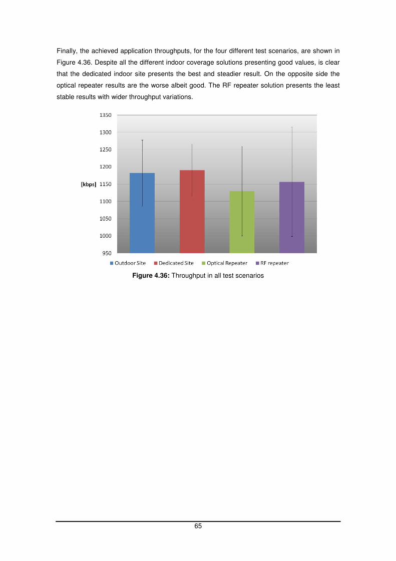
65
Finally, the achieved application throughputs, for the four different test scenarios, are shown in
Figure 4.36. Despite all the different indoor coverage solutions presenting good values, is clear
that the dedicated indoor site presents the best and steadier result. On the opposite side the
optical repeater results are the worse albeit good. The RF repeater solution presents the least
stable results with wider throughput variations.
Figure 4.36: Throughput in all test scenarios

66

67
5 Conclusions and Future Work
In this chapter the main conclusions obtained from this work are presented. Moreover some
ideas on future work that can be done within the scope of this document are also presented.
68
5.1 Conclusions The main goal of the present work was to study the real life network performance of HSUPA in
indoor environments. This goal was accomplished through the execution of several tests in
different indoor environments. The four most common indoor coverage solutions were chosen
to perform the tests: outdoor site, dedicated indoor site, optical repeater and RF repeater. On
each of the tested scenarios three test points with different radio characteristics were tested: by
the window, standard indoor location and close to the antenna. In the case of the indoor
coverage by outdoor site a deep indoor location was tested instead of the antenna location. For
each test point one HSUPA user performed successive 5 MB uploads during one hour in order
to test the achieved throughput and network impact. All these tests were performed in low
loaded cells and, as mentioned previously, with only one HSUPA user.
The main result taken from the conducted tests was that the achieved uplink application
throughput with HSUPA using category 3 UE is exceeds 1100 kbps in all scenarios and test
points, reaching almost 1200 kbps in the points presenting the best throughput. These values
can be considered as very good since the theoretical limit physical layer throughput for category
3 UE is 1,45 Mbps. It was also verified that the achieved throughput is not strongly affected by
the radio conditions, at least the ones the UE was subject during the performed tests. Alongside
with that also the technical solution to provide the indoor coverage did not play a major role in
the final throughput. It is possible to say that current implementations of HSUPA with 2SF4 and
category 3 UE achieve application throughputs of about 80% of the physical layer theoretical
maximum in most indoor environments and radio conditions.
One of the reasons for the good performance was probably the fast retransmissions with
HARQ, which is one of the new features for HSUPA. During the tests it was possible to confirm
the advantages of HARQ by observing the 1st transmission BLER values of around 10%, which
allows higher throughputs at worse radio conditions and confirm that the residual BLER was 0%
after the retransmissions without significant losses in application throughput. Moreover when
the radio conditions became worse, in all our test cases the UE was capable of compensate
that degradation with extra power and maintain the throughput level at high values. This must
be the case in a large majority of indoor environments with dedicated indoor coverage systems,
as in this cases the radio conditions are most of the time quite good if care is taken in the
system design.
Finally, the impact of an individual HSUPA user in the total cell interference is low in most test
cases. The RTWP increases during the hours where the tests were performed are in general
below 1 dB, therefore not affecting too much the NR allowance for the single cell and allowing
several simultaneous users. Care should be taken though in generalizing this conclusion as all
performed tests were made under good radio conditions, which is not always the case. The pole
69
throughput and capacity values, calculated in chapter 3, suggest that for more limit situations
the impact is significantly higher. The only test scenario where RTWP values raised by about 2
dB was the optical repeater; therefore one can expect more capacity problems with this kind of
solution for indoor coverage. It is also worth mention the fact that repeater solutions introduce
significant increases in the BTS total noise even when no UE are connected to the system. This
is not a problem in itself as capacity depends on interference rise and not absolute interference
values. However if this values become to high, unless the devices provide very good coverage
in the whole coverage area might cause the UE to reach its power limit and not be able to
sustain the signal to noise ratio needed to maintain high throughput values.
As a final conclusion from this work, it is possible to say that HSUPA bring uplink data transfers
to a new level in indoor environments, performing according to expectations whenever in
presence of a proper dedicated designed system or good coverage from outdoor sites that
provide good radio conditions. Moreover that significant throughput improvement comes at a
low price in terms of cell noise rise, again when in presence of good radio conditions.
5.2 Future Work
For future work one would recommend to perform tests with several UE to simulate a highly
loaded cell scenario. This would give a better insight on the real cell capacity and throughput
limits. Another suggestion would be to perform the tests under worse radio conditions to verify
the limitations brought by those to the HSUPA performance. Finally it is suggested to repeat the
current tests, possibly including the previous suggestions, with the new Category 5 and 6 UE as
they become available and networks support them.
On a slightly different approach one would suggest to perform full HSPA tests with simultaneous
uplink and downlink data transfers. Another possibility would be to perform multi RAB
performance tests with simultaneous data transfers and voice calls. It would also be interesting
to study how to reduce the impact of repeaters in BTS received noise power and test HSUPA in
several RF repeaters connected to a single cell.

70

71
Annex I - Propagation Models

72
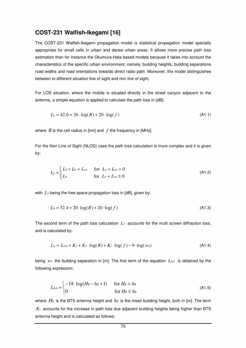
73
COST-231 Walfish-Ikegami [16] The COST-231 Walfish-Ikegami propagation model is statistical propagation model specially
appropriate for small cells in urban and dense urban areas. It allows more precise path loss
estimation than for instance the Okumura-Hata based models because it takes into account the
characteristics of the specific urban environment, namely: building heights, building separations
road widths and road orientations towards direct radio path. Moreover, the model distinguishes
between to different situation line of sight and non line of sight.
For LOS situation, where the mobile is situated directly in the street canyon adjacent to the
antenna, a simple equation is applied to calculate the path loss in [dB]:
)log(20)log(266.42 fRLp ⋅+⋅+= (A1.1)
where R is the cell radius in [km] and f the frequency in [MHz].
For the Non Line of Sight (NLOS) case the path loss calculation is more complex and it is given
by:
≤+
>+++=
0for
0for
0
0
tmtt
tmtttmtt
p
LLL
LLLLLL (A1.2)
with 0L being the free space propagation loss in [dB], given by:
)log(20)log(204.320 fRL ⋅+⋅+= (A1.3)
The second term of the path loss calculation ttL accounts for the multi screen diffraction loss,
and is calculated by:
)log(9)log()log( bfdabshtt wfKRKKLL ⋅−⋅+⋅++= (A1.4)
being bw the building separation in [m]. The first term of the equation bshL is obtained by the
following expression:
≤
>+−⋅−=
for 0
for )1log(18
BB
BBBB
bsh
hH
hHhHL (A1.5)
where BH is the BTS antenna height and Bh is the mean building height, both in [m]. The term
aK accounts for the increase in path loss due adjacent building heights being higher than BTS
antenna height and is calculated as follows:
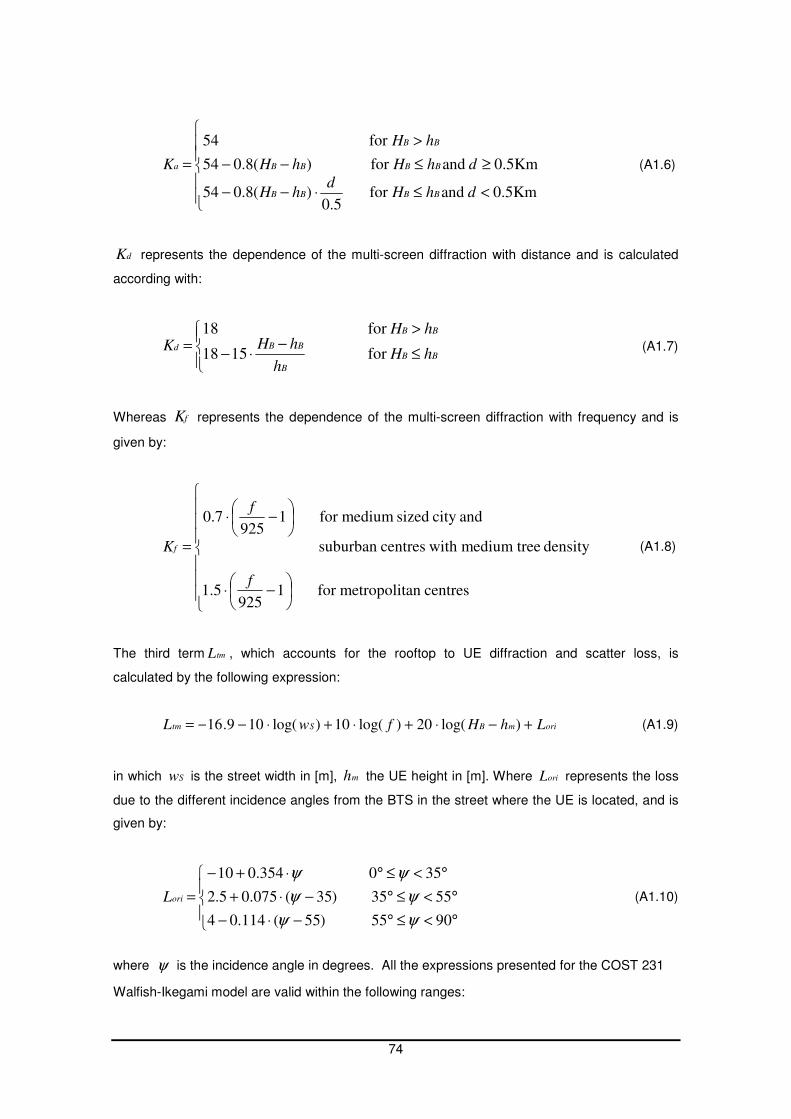
74
<≤⋅−−
≥≤−−
>
=
Km5.0 andfor 5.0
)(8.054
Km5.0 andfor )(8.054
for 54
dhHd
hH
dhHhH
hH
K
BBBB
BBBB
BB
a (A1.6)
dK represents the dependence of the multi-screen diffraction with distance and is calculated
according with:
≤−
⋅−
>=
for 1518
for 18
BB
B
BB
BB
dhH
h
hHhH
K
(A1.7)
Whereas fK represents the dependence of the multi-screen diffraction with frequency and is
given by:
−⋅
−⋅
=
centresan metropolitfor 1925
5.1
density treemedium with centressuburban
andcity sized mediumfor 1925
7.0
f
f
Kf (A1.8)
The third term tmL , which accounts for the rooftop to UE diffraction and scatter loss, is
calculated by the following expression:
orimBStm LhHfwL +−⋅+⋅+⋅−−= )log(20)log(10)log(109.16 (A1.9)
in which Sw is the street width in [m], mh the UE height in [m]. Where oriL represents the loss
due to the different incidence angles from the BTS in the street where the UE is located, and is
given by:
°<≤°−⋅−
°<≤°−⋅+
°<≤°⋅+−
=
9055 )55(114.04
5535 )35(075.05.2
350 354.010
ψψ
ψψ
ψψ
oriL (A1.10)
where ψ is the incidence angle in degrees. All the expressions presented for the COST 231
Walfish-Ikegami model are valid within the following ranges:

75
• 800 < f < 2000 [MHz]
• 4 < BH < 50 [m]
• 1 < mh < 3 [m]
• 0.02 < R < 5 [km]
COST-231 Indoor Multi Wall Model (adapted by 3GPP) [16] The COST-231 defined an indoor propagation model called Multi Wall Model, which is given by:
fwi
I
i
wicp LnLkLLLb
n
n
⋅+⋅++=
−
+
+
∑=
2
1
1
0
(A1.11)
where oL is the free space propagation in [dB]. cL is a constant loss which corrects the
values measured for the wall losses in [dB]. wik is the number of penetrated walls of type i ,
whereas wiL accounts for the loss of an individual wall type i , in [dB]. Finally, n is the number
of penetrated floors, b is an empirical parameter and fL is the loss between adjacent floors, in
[dB].
Based on that model, 3GPP adapted expression (A1.11) specifically to UMTS characteristics
arriving to the following expression:
−
+
+
⋅+⋅+⋅+= ∑=
46.02
1
3.18)log(20371
n
n
nLkRL wi
I
i
wip (A1.12)
where R is the cell radius in [m]. If walls are not individually modelled (A1.12) can be
approximated by:
−
+
+
⋅+⋅+=46.0
2
1
3.18)log(3037 n
n
nRLp
(A1.13)
which in the case of a single floor leads to the simpler:
)log(3037 RLp ⋅+= (A1.14)

76

77
Annex II - Additional Test Results

78
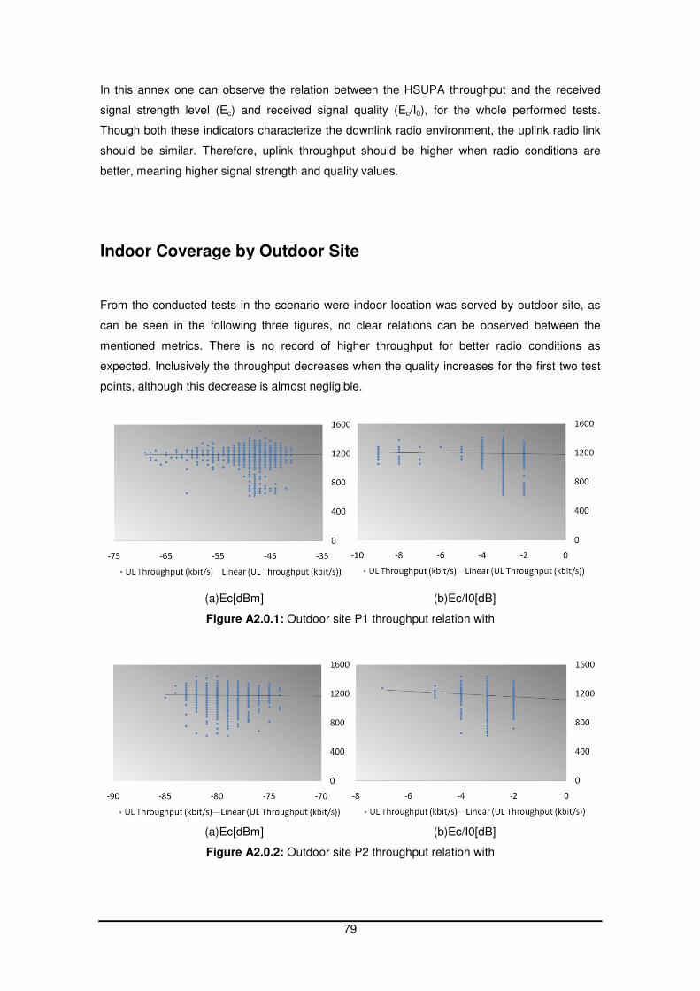
79
In this annex one can observe the relation between the HSUPA throughput and the received
signal strength level (Ec) and received signal quality (Ec/I0), for the whole performed tests.
Though both these indicators characterize the downlink radio environment, the uplink radio link
should be similar. Therefore, uplink throughput should be higher when radio conditions are
better, meaning higher signal strength and quality values.
Indoor Coverage by Outdoor Site
From the conducted tests in the scenario were indoor location was served by outdoor site, as
can be seen in the following three figures, no clear relations can be observed between the
mentioned metrics. There is no record of higher throughput for better radio conditions as
expected. Inclusively the throughput decreases when the quality increases for the first two test
points, although this decrease is almost negligible.
(a)Ec[dBm] (b)Ec/I0[dB]
Figure A2.0.1: Outdoor site P1 throughput relation with
(a)Ec[dBm] (b)Ec/I0[dB]
Figure A2.0.2: Outdoor site P2 throughput relation with
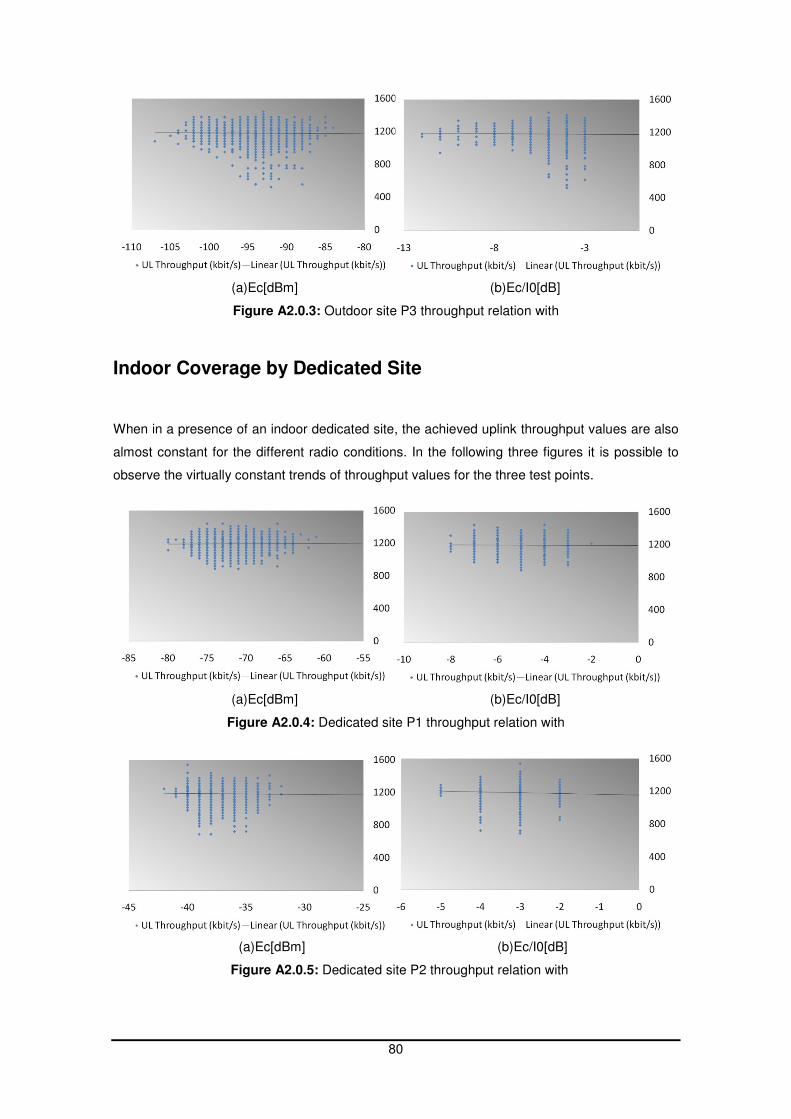
80
(a)Ec[dBm] (b)Ec/I0[dB]
Figure A2.0.3: Outdoor site P3 throughput relation with
Indoor Coverage by Dedicated Site
When in a presence of an indoor dedicated site, the achieved uplink throughput values are also
almost constant for the different radio conditions. In the following three figures it is possible to
observe the virtually constant trends of throughput values for the three test points.
(a)Ec[dBm] (b)Ec/I0[dB]
Figure A2.0.4: Dedicated site P1 throughput relation with
(a)Ec[dBm] (b)Ec/I0[dB]
Figure A2.0.5: Dedicated site P2 throughput relation with
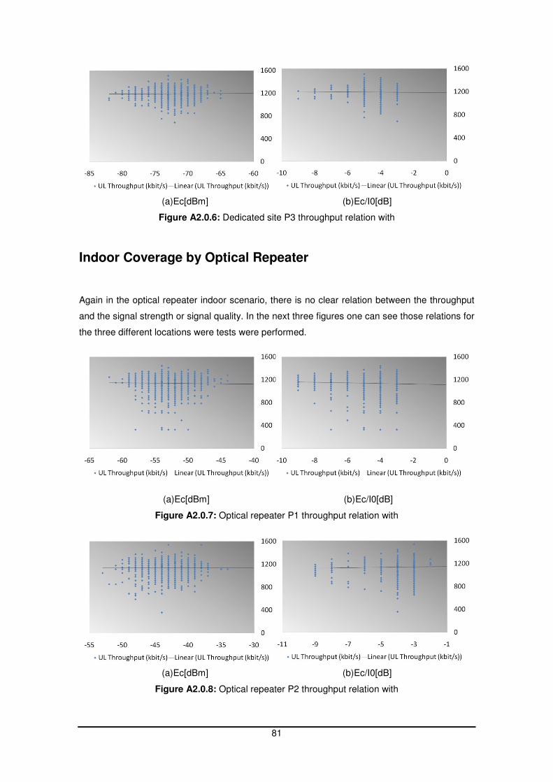
81
(a)Ec[dBm] (b)Ec/I0[dB]
Figure A2.0.6: Dedicated site P3 throughput relation with
Indoor Coverage by Optical Repeater
Again in the optical repeater indoor scenario, there is no clear relation between the throughput
and the signal strength or signal quality. In the next three figures one can see those relations for
the three different locations were tests were performed.
(a)Ec[dBm] (b)Ec/I0[dB]
Figure A2.0.7: Optical repeater P1 throughput relation with
(a)Ec[dBm] (b)Ec/I0[dB]
Figure A2.0.8: Optical repeater P2 throughput relation with

82
(a)Ec[dBm] (b)Ec/I0[dB]
Figure A2.0.9: Optical repeater P3 throughput relation with
Indoor Coverage by RF Repeater
Finally, in the following three figures one can observe the relation between uplink throughput
and the signal strength and signal quality, for the three different test points in the RF repeater
scenario. As in the previous scenarios, there is no clear relation between throughput and radio
conditions.
(a)Ec[dBm] (b)Ec/I0[dB]
Figure A2.0.10: RF repeater P1 throughput relation with
(a)Ec[dBm] (b)Ec/I0[dB]
Figure A2.0.11: RF repeater P2 throughput relation with
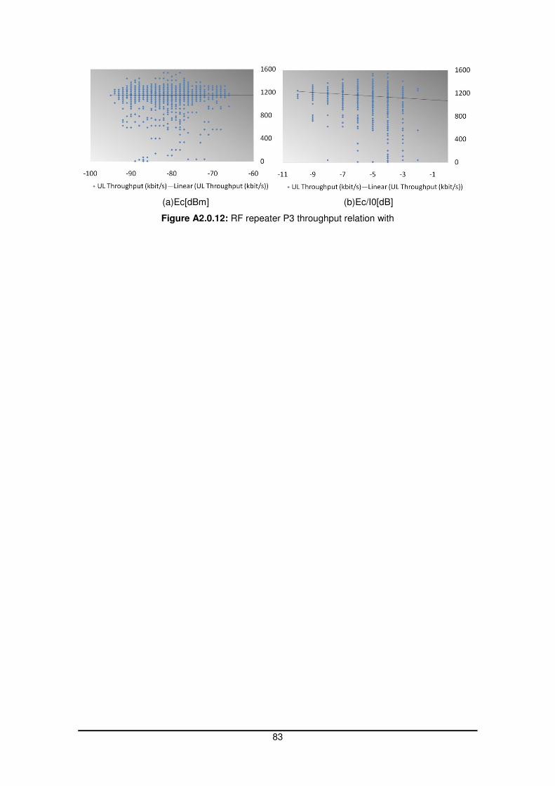
83
(a)Ec[dBm] (b)Ec/I0[dB]
Figure A2.0.12: RF repeater P3 throughput relation with

84
85
References
[1] - Stuckmann,P. and Zimmermann,R., Towards Ubiquitous and Unlimited-capacity
Communication Networks – European Research in Framework Programme 7, European
Commission, Mar 2007.
[2] - Baptista, P., Impact of HSUPA Implementation on UMTS Capacity and Cell Coverage,
M. Sc. Thesis, IST-UTL, Lisbon, Portugal, Dec 2007.
[3] - Lopes, J., Performance Analysis of UMTS/HSDPA/HSUPA at the Cellular Level, M. Sc.
Thesis, IST-UTL, Lisbon, Portugal, Mar 2008
[4]- Helmersson,K., Englund,E., Edvardsson,M., Edholm,C., Parkvall,S., Samuelsson,M.,
Wang,Y. and Cheng,J., “System Performance of WCDMA Enhanced Uplink”, in Proc. of
VTC’05 Spring – 61st
IEEE Vehicular Technology Conference, Stockholm, Sweden,
June 2005.
[5] - Aspects of HSUPA Network Planning, 80-W1159-1, Revision B, Qualcomm, 2007.
[6] - Chen,T., Kuusela,M. and Malkamaki,E., Uplink Capacity of VoIP on HSUPA, in Proc. Of
VTC’06 – 63rd IEEE Vehicular Technology Conference, Melbourne, Australia, May
2006.
[7] - Rui, F., Persson, F., Nordberg, M., Wänstedt, S. Qingyu, M., Xinyu, G., Coverage Study
for VoIP over Enhanced Uplink, Ericsson, May 2006.
[8] - 3GPP, Service Aspects, Service and service capabilities (Release 7); TS 22.105 V7.1.0,
Dec 2006 (http://www.3gpp.org).
[9] - Holma,H. and Toskala,A., WDCMA for UMTS – HSPA Evolution and LTE, Fourth
Edition, John Wiley & Sons, UK, 2007.
[10] - UMTS Forum, UMTS/IMT-2000 Spectrum, Nº6 Report from the UMTS Forum, Jun 1999
(www.umts-forum.org).
[11] - 3GPP, Physical Channels and mapping of transport channels onto physical channels
(Release 1999); TS 25.211 V3.12.0, Sep 2002 (http://www.3gpp.org).
86
[12] - Holma,H. and Toskala,A., HSDPA/HSUPA For UMTS, High Speed Radio Access for
Mobile Communications, John Wiley & Sons, UK, 2006.
[13] - 3GPP, Technical Specification Group Radio Access Network; Base Station (BS) radio
transmission and reception (FDD) (Release 7); TS 25.104 V7.11.0, Dec 2008
(http://www.3gpp.org).
[14] - Dahlman,E., Parkvall,S., Sköld,J. and Beming,P., 3G Evolution, HSPA and LTE for
Mobile Broadband, Academic Press, UK, 2007.
[15] - Laiho,J., Wacker,A. and Novosad,T., Radio Network Planning and Optimisation for
UMTS, Second Edition, John Wiley & Sons, UK, 2005.
[16] - Digital Mobile Radio Towards Future Generation Systems, COST 231 Final Report,
1999 (http://www.lx.it.pt/cost231/final_report.htm).
[17] - 3GPP, Technical Specification Group Radio Access Network; Base Station (BS)
conformance testing (FDD) (Release 7); TR 25.141 V7.12.0, Dec 2008
(http://www.3gpp.org).
[18] - 3GPP, Technical Specification Group Radio Access Network; FDD Base Station (BS)
classification (Release 6); TR 25.951 V6.3.0, Oct 2006 (http://www.3gpp.org).
[19] - http://www.ericsson.com/solutions/tems/index.shtml
[20] - 3GPP, Technical Specification Group Radio Access Network; User Equipment (UE)
radio transmission and reception FDD (Release 7); TS 25.101 V7.14.0, Dec 2008
(http://www.3gpp.org).


![[Job training] hsdpa+hsupa](https://img.pdfslide.net/doc/110x75/58e7b4ac1a28abbb4e8b5297/job-training-hsdpahsupa.jpg)