2005-42Final Report

IDENTIFICATION OF CAUSAL FACTORS AND POTENTIAL COUNTERMEASURES

FOR FATAL RURAL CRASHES

Technical Report Documentation Page 1. Report No. 2. 3. Recipients Accession No. MN/RC-2005-42 4. Title and Subtitle 5. Report Date

October 2005 6.

IDENTIFICATION OF CAUSAL FACTORS AND POTENTIAL COUNTERMEASURES FOR FATAL RURAL CRASHES 7. Author(s) 8. Performing Organization Report No. Gary A. Davis, Jianping Pei, Paul Morris 9. Performing Organization Name and Address 10. Project/Task/Work Unit No.

11. Contract (C) or Grant (G) No.

Dept. of Civil Engineering University of Minnesota 500 Pillsbury Drive SE Minneapolis, MN 55455

(c) 81655 (wo) 39

12. Sponsoring Organization Name and Address 13. Type of Report and Period Covered Final Report 14. Sponsoring Agency Code

Minnesota Department of Transportation 395 John Ireland Boulevard Mail Stop 330 St. Paul, Minnesota 55155 15. Supplementary Notes http://www.lrrb.org/PDF/200542.pdf 16. Abstract (Limit: 200 words) This project was divided into three phases. In phase 1 ten fatal run-off-road crashes were reconstructed from crash scene diagrams and investigation reports. We found evidence of excessive speed in five of these, and a failure to properly use seatbelts eight of the ten. For seven of these we found that barriers complying with Test Level 3 of NCHRP Report 350 would probably have stopped the crashing vehicle’s encroachment. In phase 2 we developed a vehicle trajectory simulation model and used it reconstruct five fatal median-crossing crashes. We found clear evidence of excessive speed in one of these, and in three of the five the encroaching vehicle would probably have been restrained by Test Level 3-compliant barriers. In phase 3 five teams of traffic safety professionals reviewed accident reports from a sample of fatal rural crashes, with the aim of identifying possible causal factors and potential countermeasures. The most frequently identified causal factors were driver inexperience and failure to properly use restraints, while provision of rumble strips, improvements to roadsides or cross-slopes, and provision of guardrails or barriers were the most frequently-cited countermeasures. 17. Document Analysis/Descriptors 18. Availability Statement Crash Reconstruction Roadway Departure Crashes

Bayesian Analysis Fatal Crashes Gibbs Sampling

No restrictions. Document available from: National Technical Information Services, Springfield, Virginia 22161

19. Security Class (this report) 20. Security Class (this page) 21. No. of Pages 22. Price Unclassified Unclassified 71

IDENTIFICATION OF CAUSAL FACTORS AND POTENTIAL COUNTERMEASURES FOR

FATAL RURAL CRASHES

Final Report

Prepared by:

Gary A. Davis Jianping Pei Paul Morris

Department of Civil Engineering

University of Minnesota

October 2005

Published by:

Minnesota Department of Transportation Research Services Section

Mail Stop 330 395 John Ireland Boulevard

St. Paul, Minnesota 55155-1899

This report represents the results of research conducted by the authors and does no necessarily represent the view or policy of the Minnesota Department of Transportation and/or the Center for Transportation Studies. This report does not contain a standard or specified technique.

Acknowledgments

We would like to thank Marc Briese and Loren Hill for their guidance and assistance in making this research possible. We would also like to thank the members of our expert panels for giving their time to support this project: Name Organization Eil Kwon Minnesota Dept. of Transportation Loren Hill Minnesota Dept. of Transportation Ning Li Minnesota Dept. of Transportation Ben Johnson Minnesota Dept. of Transportation Robert Ege Minnesota Dept. of Transportation Jolene Servatius Minnesota Dept. of Transportation Gary Dirlam Minnesota Dept. of Transportation Marc Flygare Minnesota Dept. of Transportation Marj Ebersteiner Minnesota Dept. of Transportation Lesa Monroe Minnesota Dept. of Transportation Monty Eidem Minnesota Dept. of Transportation Janelle Fowlds Minnesota Dept. of Transportation Tina Folch Minnesota Dept. of Public Safety Alan Rodgers Minnesota Dept. of Public Safety Gordy Pehrson Minnesota Dept. of Public Safety Kathleen Haney Minnesota Dept. of Public Safety Kathy Burke Moore Minnesota Dept. of Public Safety Mark Sprengeler Minnesota State Patrol Jay Engeswick Minnesota State Patrol Paul Skoglund Minnesota State Patrol Dan McBroom Minnesota State Patrol Mark Tauzell Minnesota State Patrol

Table of Contents Chapter One: Introduction: What Do We Mean by Cause? 1 Chapter Two: Primarily Roll-Over Crashes 3 2.1 Background 3 2.2 Scope of Reconstruction 4 2.3 Uncertainty in Crash Reconstruction 6 2.4 Reconstruction of (Primarily) Rollover Crashes 7 2.5 Effect of Hypothetical Barrier Placements 10 2.6 Discussion 11 Chapter Three: Median-Crossing Crashes 13 3.1 Background 13 3.2 Gibbs Sampling 13 3.3 Reconstruction of Median-Crossing Crashes 15 3.3.1 Setting Up the Reconstructions 16 3.3.2 Actual Reconstructions 17 3.4 Discussion 31 Chapter Four: Expert Assessment of Extended Sample 33 4.1 Review of Clinical Crash Assessment 33 4.2 Selection of Assessment Methodology 34 4.3 Drawing the Extended Sample and Forming the Expert Panel 36 4.4 Data Reduction and Analysis 37 4.5 Results 39 4.6 Discussion 42 Chapter Five: Summary and Conclusions 45 References 47 Appendix A: WinBUGS Model for Rollover Crash 7 A-1 Appendix B: Handout Provided to Expert Panel Participants B-1

List of Tables Table 2.1 Accident Type Codes for Crashes in Initial Sample 3 Table 2.2 Accident Diagram Codes for Crashes in Initial Sample 4 Table 2.3 Characteristics of 10 Roadway Departure Crashes 8 Table 2.4 Summary of Speed and Impact Severity Estimates for 10 Run-off- 9 road Cases Table 2.5 Additional Summary of Ten Fatal Run-off Road Crashes 12 Table 3.1 Diagnostic Points in Crash One 18 Table 3.2 Bounds of Prior Distributions for Inputs: Crash One 18 Table 3.3 Gelman-Rubin Statistics for Crash One 19 Table 3.4 Statistics of Posterior Distributions for Inputs in Crash One 19 Table 3.5 Impact Severity Statistics for Crash One 21 Table 3.6 Diagnostic Points in Crash Two 22 Table 3.7 Bounds of Prior Distributions for Inputs in Crash Two 22 Table 3.8 Gelman-Rubin Statistics for Crash Two 23 Table 3.9 Statistics of Posterior Distributions for Inputs in Crash Two 23 Table 3.10 Impact Severity Statistics for Crash Two 24 Table 3.11 Diagnostic Points for Crash Three 25 Table 3.12 Bounds of Prior Distribution for Inputs in Crash Three 25 Table 3.13 Gelman-Rubin Statistics for Crash Three 25 Table 3.14 Statistics of Posterior Distributions for Inputs into Crash Three 25 Based on 25000 'Consistent' Iterations Table 3.15 Impact Severity Statistics for Crash Three 26 Table 3.16 Diagnostic Points in Crash Four 27

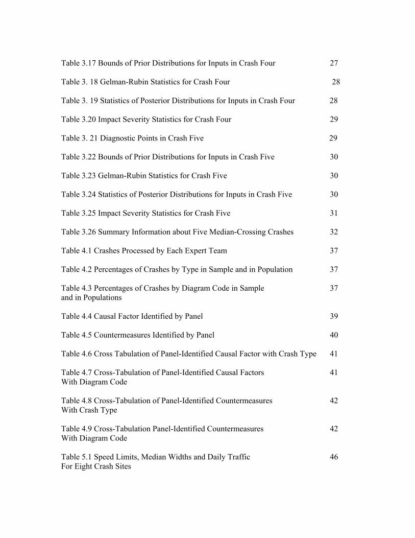
Table 3.17 Bounds of Prior Distributions for Inputs in Crash Four 27 Table 3. 18 Gelman-Rubin Statistics for Crash Four 28 Table 3. 19 Statistics of Posterior Distributions for Inputs in Crash Four 28 Table 3.20 Impact Severity Statistics for Crash Four 29 Table 3. 21 Diagnostic Points in Crash Five 29 Table 3.22 Bounds of Prior Distributions for Inputs in Crash Five 30 Table 3.23 Gelman-Rubin Statistics for Crash Five 30 Table 3.24 Statistics of Posterior Distributions for Inputs in Crash Five 30 Table 3.25 Impact Severity Statistics for Crash Five 31 Table 3.26 Summary Information about Five Median-Crossing Crashes 32 Table 4.1 Crashes Processed by Each Expert Team 37 Table 4.2 Percentages of Crashes by Type in Sample and in Population 37 Table 4.3 Percentages of Crashes by Diagram Code in Sample 37 and in Populations Table 4.4 Causal Factor Identified by Panel 39 Table 4.5 Countermeasures Identified by Panel 40 Table 4.6 Cross Tabulation of Panel-Identified Causal Factor with Crash Type 41 Table 4.7 Cross-Tabulation of Panel-Identified Causal Factors 41 With Diagram Code Table 4.8 Cross-Tabulation of Panel-Identified Countermeasures 42 With Crash Type Table 4.9 Cross-Tabulation Panel-Identified Countermeasures 42 With Diagram Code Table 5.1 Speed Limits, Median Widths and Daily Traffic 46 For Eight Crash Sites

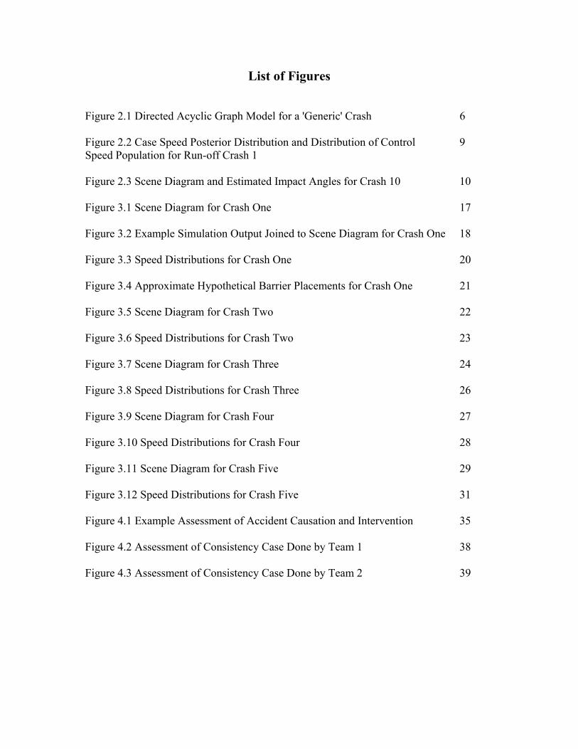
List of Figures Figure 2.1 Directed Acyclic Graph Model for a 'Generic' Crash 6 Figure 2.2 Case Speed Posterior Distribution and Distribution of Control 9 Speed Population for Run-off Crash 1 Figure 2.3 Scene Diagram and Estimated Impact Angles for Crash 10 10 Figure 3.1 Scene Diagram for Crash One 17 Figure 3.2 Example Simulation Output Joined to Scene Diagram for Crash One 18 Figure 3.3 Speed Distributions for Crash One 20 Figure 3.4 Approximate Hypothetical Barrier Placements for Crash One 21 Figure 3.5 Scene Diagram for Crash Two 22 Figure 3.6 Speed Distributions for Crash Two 23 Figure 3.7 Scene Diagram for Crash Three 24 Figure 3.8 Speed Distributions for Crash Three 26 Figure 3.9 Scene Diagram for Crash Four 27 Figure 3.10 Speed Distributions for Crash Four 28 Figure 3.11 Scene Diagram for Crash Five 29 Figure 3.12 Speed Distributions for Crash Five 31 Figure 4.1 Example Assessment of Accident Causation and Intervention 35 Figure 4.2 Assessment of Consistency Case Done by Team 1 38 Figure 4.3 Assessment of Consistency Case Done by Team 2 39

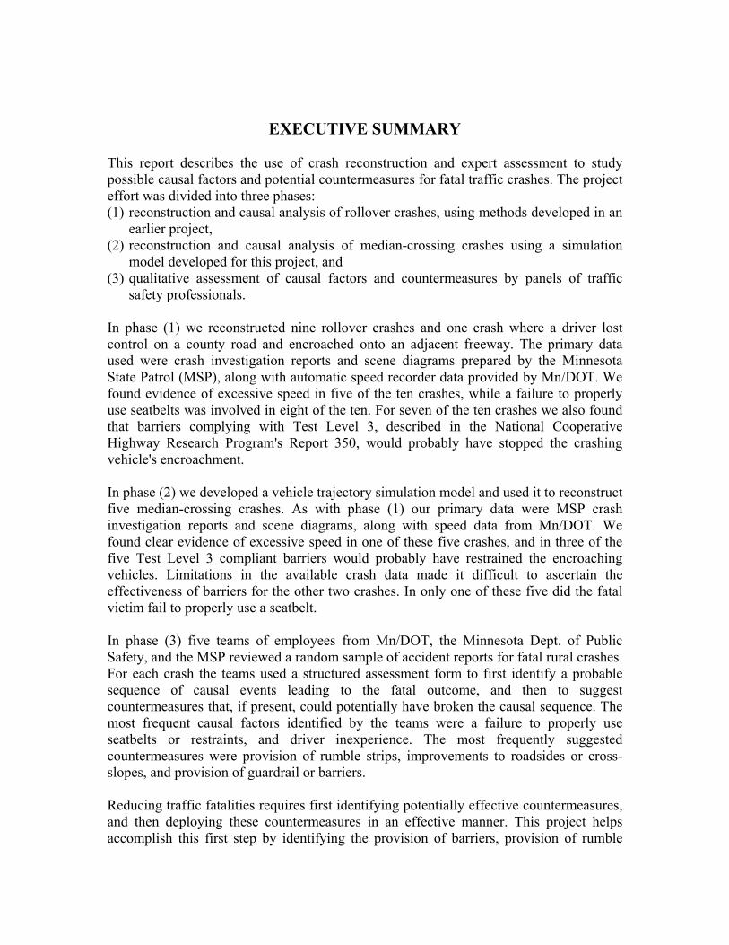
EXECUTIVE SUMMARY This report describes the use of crash reconstruction and expert assessment to study possible causal factors and potential countermeasures for fatal traffic crashes. The project effort was divided into three phases: (1) reconstruction and causal analysis of rollover crashes, using methods developed in an

earlier project, (2) reconstruction and causal analysis of median-crossing crashes using a simulation

model developed for this project, and (3) qualitative assessment of causal factors and countermeasures by panels of traffic

safety professionals. In phase (1) we reconstructed nine rollover crashes and one crash where a driver lost control on a county road and encroached onto an adjacent freeway. The primary data used were crash investigation reports and scene diagrams prepared by the Minnesota State Patrol (MSP), along with automatic speed recorder data provided by Mn/DOT. We found evidence of excessive speed in five of the ten crashes, while a failure to properly use seatbelts was involved in eight of the ten. For seven of the ten crashes we also found that barriers complying with Test Level 3, described in the National Cooperative Highway Research Program's Report 350, would probably have stopped the crashing vehicle's encroachment. In phase (2) we developed a vehicle trajectory simulation model and used it to reconstruct five median-crossing crashes. As with phase (1) our primary data were MSP crash investigation reports and scene diagrams, along with speed data from Mn/DOT. We found clear evidence of excessive speed in one of these five crashes, and in three of the five Test Level 3 compliant barriers would probably have restrained the encroaching vehicles. Limitations in the available crash data made it difficult to ascertain the effectiveness of barriers for the other two crashes. In only one of these five did the fatal victim fail to properly use a seatbelt. In phase (3) five teams of employees from Mn/DOT, the Minnesota Dept. of Public Safety, and the MSP reviewed a random sample of accident reports for fatal rural crashes. For each crash the teams used a structured assessment form to first identify a probable sequence of causal events leading to the fatal outcome, and then to suggest countermeasures that, if present, could potentially have broken the causal sequence. The most frequent causal factors identified by the teams were a failure to properly use seatbelts or restraints, and driver inexperience. The most frequently suggested countermeasures were provision of rumble strips, improvements to roadsides or cross-slopes, and provision of guardrail or barriers. Reducing traffic fatalities requires first identifying potentially effective countermeasures, and then deploying these countermeasures in an effective manner. This project helps accomplish this first step by identifying the provision of barriers, provision of rumble

strips, and roadside/cross-slope improvements as potentially effective roadway-related countermeasures. The second step is arguably the more difficult, and is analogous to effectively using a flu vaccine. Deciding who should receive the vaccine in light of a limited supply, potential side effects, and differential susceptibility to the flu virus is clearly more difficult than determining who might have survived the flu had they been vaccinated. Similarly, a decision to install guardrail on a section of highway in response to a median-crossing fatality should consider that resource constraints will limit the number of sections that can be treated, that maintenance costs will be probably be incurred, and that traffic or speed conditions on other sections may make them more susceptible to median-crossing events. This in essence requires that we be able to predict the costs and benefits of applying the countermeasure at actual, individual highway locations, and brings us to the frontier of traffic safety research. Methods do exist for predicting costs and benefits for some countermeasure types, such as intersection signalization or removal of fixed roadside objects, but not, at present, for the three countermeasures identified in this research. Research into and development of the required prediction models is the next step toward implementation.

1

CHAPTER ONE INTRODUCTION: WHAT DO WE MEAN BY ‘CAUSE’?

As the title indicates, a primary focus of this project is on identification of probable causes of fatal road crashes. The late Stan Baker has pointed out that in traffic safety the word ‘cause’ is often invoked to achieve rhetorical or legal, rather than scientific, objectives (1975), and the philosopher Nancy Cartwright (2002) has argued that what we mean by 'cause' often varies across different contexts. It may be useful then to be clear about we mean by 'causal factor' in this study, and how we determine whether or not an event is a causal factor for a crash. A rough-and-ready knowledge of the causal structure of our day-to-day world is essential for survival, and most animals (humans included) manage to acquire this without recourse to an explicit theory of causation. The source of this knowledge, as the philosopher David Hume pointed out, is our experience with our world. "Thus we remember to have seen that species of object we call flame, and to have felt that species of sensation we call heat…without any farther ceremony we call the one cause and the other effect." (quoted in Pearl 2000). That is, our knowledge of the causal relations between events comes from observing their conjunction. A little thought, though, reveals that this is not enough. The length of a shadow varies with the height of the sun, but does the sun's height cause the shadow's length or does the shadow's length cause the sun's height? A drunk driver is rear-ended while stopped at a red light. If investigated, this crash would probably be recorded as 'alcohol involved' but was alcohol intoxication a cause of the crash? Or, to use another phrase we've all heard "association does not imply causation." So if association (alone) is not causation, what is? David Hume had an answer to this question: "..we may define a cause to be an object, followed by another, and where all objects similar to the first are followed by objects similar to the second. Or in other words where, if the first object had not been, the second never had existed." (1748/1958). Stan Baker has expressed a similar idea, in more modern language, in his definition of a 'causal factor' as a circumstance "contributing to a result without which the result could not have occurred" (1975). The National Transportation Safety Board (NTSB) expressed a similar idea in its definition of 'probable cause' as a "condition or event" such that "had the condition or event been prevented…the accident would not occur." In essence then, we say event A caused event B if

(1) Event A occurred, (2) Event B occurred, (3) If A hadn't occurred, neither would have B.

Statements (1) and (2) are of a sort we can in principle verify through observation. The rear-ending crash was observed to occur, and the blood alcohol of the rear-ended driver was 0.20. Statement (3) though is an example of what philosophers call a 'counterfactual conditional’; a statement about what would have happened had things been different. Because it is a statement about things, which did not occur, there is no direct observation we can make to verify its truth. The statistician Paul Holland has called this difficulty the "Fundamental Problem of Causal Inference" (Holland 1986). Obviously though we have managed to develop reasonably useful causal knowledge about at least some aspects of our universe so it must be possible, at least sometimes, to solve this problem.

2

As Holland points out, much of our scientific progress comes from using controlled experiments to test and verify causal claims. In essence we set up a situation where event A occurs and another where event A does not occur, and look to see when event B occurs. The plausibility of our causal conclusion then hinges on whether or not the only thing that changes in these two situations is the occurrence or non-occurrence of event A. When strict control of all relevant factors is not possible statistical control, which aims to determine whether or not statement (3) is true 'on average' rather than for any individual case, can still be achieved by randomly determining, for a group of similar situations, whether or not event A occurs. For road crashes, and accidents more generally, we are interested in the causal connection in a specific occurrence of A and B. However, the complexity of the original crash occurrence prevents us from replicating it in a laboratory. In such cases we are often willing to rely on the opinion of an expert as to whether or not statement (3) is plausible. For example, a medical examiner determines (B) that a person is dead, and (A) there is a bullet wound in that person's head, and then asserts (often implicitly) that if the bullet hadn't entered the person's head, other things equal, that person would not have died. In some situations it is possible to develop and support an expert opinion through the use of simulation. Here, one must first have a plausible mathematical model of how causal processes operate in a situation. One can then use the model to simulate what would be observed if one were to conduct a controlled experiment. For example, the National Transportation Safety Board uses flight simulators to test if particular pilot actions were causes of aircraft crashes. A technically simpler, but logically similar, example is the use of simple braking equations to test whether a high vehicle speed was a causal factor in a vehicle-pedestrian collision (Davis 1999). In this report we will use both approaches to study some possible causal factors and potential countermeasure for fatal traffic crashes. Special, but not exclusive, attention will be given to the role of speed as a causal factor and to the potential effectiveness of barriers as countermeasures. Chapter Two begins with an overview of our approach to crash reconstruction and causal analysis, and then applies this approach to ten fatal run-off-road crashes. Chapter Three takes up median-crossing crashes and begins by describing a vehicle trajectory simulator developed for this project. The simulator is then coupled with a statistical method called Gibbs sampling, and we use this tool to analyze five median-crossing crashes. Chapter Four then describes an expert panel study conducted to identify causal factors and countermeasures for a larger sample of crashes than we could analyze using reconstruction. Finally Chapter Five summarizes our findings and presents some general conclusions.

3

CHAPTER TWO

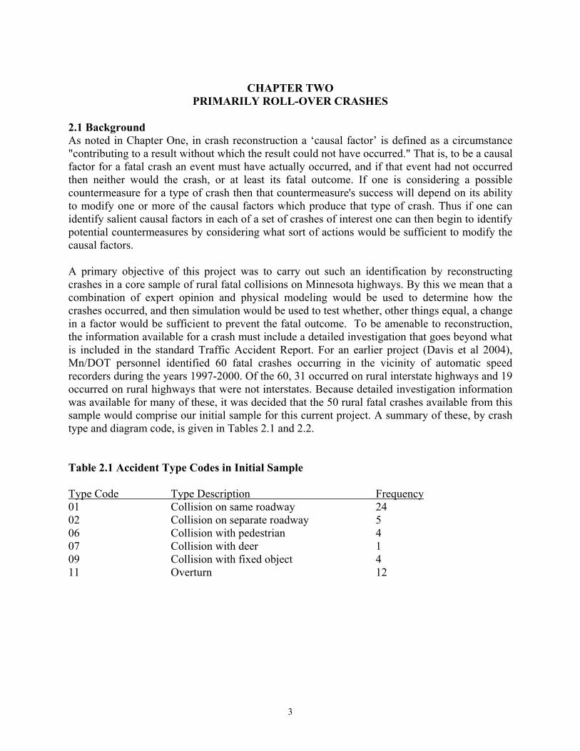
PRIMARILY ROLL-OVER CRASHES 2.1 Background As noted in Chapter One, in crash reconstruction a ‘causal factor’ is defined as a circumstance "contributing to a result without which the result could not have occurred." That is, to be a causal factor for a fatal crash an event must have actually occurred, and if that event had not occurred then neither would the crash, or at least its fatal outcome. If one is considering a possible countermeasure for a type of crash then that countermeasure's success will depend on its ability to modify one or more of the causal factors which produce that type of crash. Thus if one can identify salient causal factors in each of a set of crashes of interest one can then begin to identify potential countermeasures by considering what sort of actions would be sufficient to modify the causal factors. A primary objective of this project was to carry out such an identification by reconstructing crashes in a core sample of rural fatal collisions on Minnesota highways. By this we mean that a combination of expert opinion and physical modeling would be used to determine how the crashes occurred, and then simulation would be used to test whether, other things equal, a change in a factor would be sufficient to prevent the fatal outcome. To be amenable to reconstruction, the information available for a crash must include a detailed investigation that goes beyond what is included in the standard Traffic Accident Report. For an earlier project (Davis et al 2004), Mn/DOT personnel identified 60 fatal crashes occurring in the vicinity of automatic speed recorders during the years 1997-2000. Of the 60, 31 occurred on rural interstate highways and 19 occurred on rural highways that were not interstates. Because detailed investigation information was available for many of these, it was decided that the 50 rural fatal crashes available from this sample would comprise our initial sample for this current project. A summary of these, by crash type and diagram code, is given in Tables 2.1 and 2.2. Table 2.1 Accident Type Codes in Initial Sample Type Code Type Description Frequency 01 Collision on same roadway 24 02 Collision on separate roadway 5 06 Collision with pedestrian 4 07 Collision with deer 1 09 Collision with fixed object 4 11 Overturn 12

4

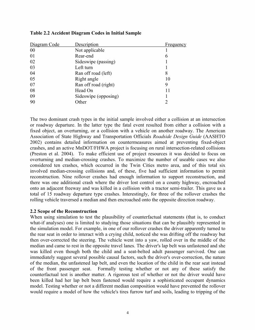
Table 2.2 Accident Diagram Codes in Initial Sample Diagram Code Description Frequency 00 Not applicable 1 01 Rear-end 6 02 Sideswipe (passing) 1 03 Left turn 1 04 Ran off road (left) 8 05 Right angle 10 07 Ran off road (right) 9 08 Head On 11 09 Sideswipe (opposing) 1 90 Other 2 The two dominant crash types in the initial sample involved either a collision at an intersection or roadway departure. In the latter type the fatal event resulted from either a collision with a fixed object, an overturning, or a collision with a vehicle on another roadway. The American Association of State Highway and Transportation Officials Roadside Design Guide (AASHTO 2002) contains detailed information on countermeasures aimed at preventing fixed-object crashes, and an active MnDOT/FHWA project is focusing on rural intersection-related collisions (Preston et al. 2004). To make efficient use of project resources it was decided to focus on overturning and median-crossing crashes. To maximize the number of useable cases we also considered ten crashes, which occurred in the Twin Cities metro area, and of this total six involved median-crossing collisions and, of these, five had sufficient information to permit reconstruction. Nine rollover crashes had enough information to support reconstruction, and there was one additional crash where the driver lost control on a county highway, encroached onto an adjacent freeway and was killed in a collision with a tractor semi-trailer. This gave us a total of 15 roadway departure type crashes. Interestingly, for three of the rollover crashes the rolling vehicle traversed a median and then encroached onto the opposite direction roadway. 2.2 Scope of the Reconstruction When using simulation to test the plausibility of counterfactual statements (that is, to conduct what-if analyses) one is limited to studying those situations that can be plausibly represented in the simulation model. For example, in one of our rollover crashes the driver apparently turned to the rear seat in order to interact with a crying child, noticed she was drifting off the roadway but then over-corrected the steering. The vehicle went into a yaw, rolled over in the middle of the median and came to rest in the opposite travel lanes. The driver's lap belt was unfastened and she was killed even though both the child and a seat-belted adult passenger survived. One can immediately suggest several possible causal factors, such the driver's over-correction, the nature of the median, the unfastened lap belt, and even the location of the child in the rear seat instead of the front passenger seat. Formally testing whether or not any of these satisfy the counterfactual test is another matter. A rigorous test of whether or not the driver would have been killed had her lap belt been fastened would require a sophisticated occupant dynamics model. Testing whether or not a different median composition would have prevented the rollover would require a model of how the vehicle's tires furrow turf and soils, leading to tripping of the

5

vehicle. Sophisticated occupant-dynamics models do exist, but to our knowledge there does not yet exist a good model of tire/soil interaction. In either case, using the detailed model would require information on the vehicle, the median, and/or driver at a level of detail not available in our crash investigations. Given that we would be limited in what types of causal factors we could test, our tactic was to study the available crash information, compare this to what our available models required, and look for opportunities to test hypotheses about crash causation. Two possibilities that revealed themselves were: (1) the role of high speed in the initiation of the crashes and (2) the potential role of roadside barriers to prevent the crashes. For the first, as noted above each of the crashes in the initial sample occurred near a Mn/DOT automatic speed recorder, so it was possible in many cases to obtain data on the speeds of vehicles using the same roadway at about the same time as the crashing vehicle. If the crashing drivers were travelling at speeds substantially higher than those of other, non-crashing drivers, this would indicate that enforcement or other countermeasures aimed at eliminating speeding 'outliers' could be an effective tactic. On the other hand if there was little difference between the speeds of crashing and non-crashing drivers this would indicate, absent a general reduction in speeds, a need for some form of roadway countermeasure, aimed at mitigating the effects of crashes once they occur. As to roadside barriers, the provision of clear zones with relatively gentle cross slopes has arguably reduced the frequency of fixed object collisions and gravity-induced rollovers. This in turn means that the relative frequency of median-crossing collisions and soil-tripped rollovers in fatal collisions has increased. At present there does not appear to be a consensus on what countermeasures to employ to reduce these types of fatalities, but increasingly transportation agencies are looking at using barriers as a countermeasure (BMI 2003). There is some uncertainty concerning the potential effectiveness of cable guardrail for preventing median-crossing crashes. Many cable-type guardrails are designed to withstand a crash at what the National Cooperative Highway Research Program's Report 350 (NCHRP 350) calls Test Level 3, which is roughly what one would expect from an unloaded pickup truck traveling at 60 mph striking the barrier at a 25 degree angle. Clearly, if run-off vehicles tend to travel at higher speeds and/or strike the barrier at higher angles then the usefulness of such barriers in stopping these vehicles before they either overturn or encroach onto opposite direction roadways, can be questioned. If it were possible from a reconstruction to identify a run-off vehicle's path, along with its speed and heading along this path then it should be possible to estimate its impact severity at hypothetical barrier locations. Comparing this impact severity to NCHRP 350's Test Level 3 should then allow us to determine whether or not a barrier would have been able to stop the vehicle had it been in place. In the remainder of this chapter we will first briefly discuss the role of uncertainty in crash reconstruction, and then turn to the reconstruction, speed estimation and barrier testing for the ten crashes that did not involve median-crossing collisions. In Chapter Three we take up the problem of reconstructing and analyzing the median-crossing crashes. The next section, 2.3, outlines the Bayesian approach to uncertain crash reconstruction. Readers more interested in our results can skip to section 2.4.

6

2.3 Uncertainty in Crash Reconstruction Crash reconstruction as often practiced using more or less deterministic methods, but increasingly crash reconstructionists are recognizing that often some degree of uncertainty is often present and that this uncertainty should, when possible, be assessed (Brach and Brach 2005, chapter 1). The Principal Investigator (PI) for this project has been developing, over the past several years, a general approach to uncertain crash reconstruction using Bayesian network methods, and a detailed presentation of his approach has been given in Davis (2003). Here we briefly outline its main features.

Figure 2.1. Directed Acyclic Graph Model for a Generic Crash.

The key to this approach is Judea Pearl's (2000) notion of a structural model, which consists of a set of background variables, a set of endogenous variables, and for each endogenous variable, a structural equation describing how that variable changes in response to changes in other model variables. The dependencies in the model can be summarized using a directed acyclic graph (DAG), where the nodes of the graph represent the model's variables, while a directed arrow from a node A to a node B indicates that A is an argument in B's structural equation. A structural equation thus encodes prior knowledge about the causal dependency of B on A. Figure 2.1 shows a DAG for a generic crash, where v denotes a vehicle's speed, z and u denote other background variables, and y takes on the value 1 if the crash occurs, and 0 otherwise. The types of variables appearing in the model and the form of the structural equation will depend on the type of crash under consideration. The variable e denotes the evidence available about the crash. If one were carrying out a reconstruction of this crash, one would begin with the evidence, then attempt to identify the structural equations relating e to v and u, and then attempt to work back to estimates for v and/or u. Uncertainty concerning the crash can be captured by specifying a probability distribution for the values taken on by the background variables, producing what Pearl calls a probabilistic causal model. The Bayesian approach to accident reconstruction then involves using the evidence and Bayes theorem to compute posterior distributions for the background variables. Now imagine we know that the vehicle's speed prior to the crash was v1, and we are interested in determining whether or not this was a cause of the crash. As we have indicated earlier, Baker has defined a "causal factor" as a circumstance "contributing to a result without which that result would not have occurred." This suggests that for the event v=v1 to count as a causal factor for a crash there must exist some other plausible speed v2 such that, other thing equal, had the vehicle

v

uy

e

v=v*

yv=v*

z

7

been travelling at speed v2 instead of v1 the crash would not have occurred. That is, we compare what happened to what would have happened in a counterfactual situation. Pearl's structural model approach can be used to implement counterfactual tests by setting the speed to some other value v2, keeping all other background variables at their original values, and then solving the structural equation for y. For the majority of crashes however precise knowledge concerning the values taken on by the background variables will not be available, so the conclusion as to whether or not v=v1 was a causal factor will be to some extent uncertain. Pearl defines a probabilistic version of the notion of causal factor using the idea of probability of necessity (PN). If we let yv=v2 denote the value taken on by y when v is set to v2, probability of necessity is then defined as PN (v1, v2) = P [yv=v2=0 | y=1 & v=v1] (2.1) (e.g. Pearl 2000, pp. 206, 286). In other words, PN is the probability the crash would not have occurred had the initial speed been v2, given that the crash did in fact occur and the initial speed was v1. In most cases however, the original speed will also not be known with certainty, and so a more useful measure of causal effect is what Pearl has called probability of disablement, but which we will call probability of avoidance PA(v2) = ∫PN(v1,v2)dF(v1|y=1, e) (2.2) In essence, computing probabilities of necessity and avoidance involves first using Bayes theorem to compute posterior probabilities for the model's background variables, then setting the speed to a target value v2, and finally computing the probability that y=0 using this posterior distribution. When a complete structural model can be specified, the Twin Network method described in Balke and Pearl (1994) can be used to carry this out, by performing Bayesian updating on an augmented network where nodes have been added to reflect the counterfactual situation. Figure 2.1 illustrates these with nodes v* and y* standing for the counterfactual situation where the speed v is set to v*. An application of this approach to vehicle/pedestrian and two-vehicle intersection crashes has been presented in (Davis 2003). 2.4 Reconstruction of (Primarily) Rollover Crashes Table 2.3 summarizes information about the 10 run-off-road cases we are considering here. For crashes 4 and 9 it was possible to measure the radius of the vehicle's path near the start of its yaw and then use the critical speed formula (Fricke 1990) to estimate the vehicle's initial speed. For five of the crashes (1,2,7,8,10) the tripped rollover model described in Cooperrider et al. (1990), Martinez and Schlueter (1996) was adapted to estimate initial speeds. In this model the vehicle's total trajectory is divided into a rolling phase, a tripping phase, and a pre-tripping phase. Each vehicle's change in speed during the rolling phase was estimated from a measurement of the distance rolled together with background knowledge of typical deceleration rates, while the change in speed during the tripping phase was estimated by first computing the force needed to trip the vehicle, converting this to its corresponding deceleration, and then combining this with prior information on the duration of tripping phases (Cooperrider et al. 1990). For the pre-tripping phase the yaw marks from the scene diagram were used to determine the vehicle's trajectory and how the vehicle's slip angle changed during this trajectory. Change in speed was then computed using friction-based deceleration rates. For the three remaining crashes

8

straightforward application of either the yaw-mark method or the rollover model was not possible but special features of the crashes were exploited in order to produce initial speed estimates. For number 3, where the driver was thrown from the rolling vehicle when it struck a fence, a Searle's (1993) pedestrian throw model was used to estimate the vehicle's speed when hitting the fence. For number 5 the fall equation was applied to a point where the vehicle went airborne over a ditch, while for number 9 the critical speed formula was used to estimate the initial speed of the rear-ended vehicle, and then a braking and yaw model was used to estimate the initial speed of the rear-ending vehicle. Table 2.3 Characteristics of 10 Roadway Departure Crashes Crash Number

LCR Number Date Time Weather/ Road

Outcome

1 00100019 01/01/2000 7:44 PM Snowy Run-off right/ rollover 2 00100672 02/04/2000 1:30 AM Snowy Run-off right/ rollover 3 00404813 04/02/2000 6:24 PM Wet Run-off right/ rollover 4 97406751 06/01/1997 12:40 AM Dry Run-off right/ rollover 5 98601665 04/10/1998 1:47 PM Dry Run-off right/

collision on adjacent freeway

6 99104860 10/22/1999 6:30 PM Dry Run-off left/ rollover 7 99105543 11/29/1999 6:06 AM Dry Deer hit, run-off left/

rollover 8 99417595 12/25/1999 12:28 PM Dry Run-off left/ rollover 9 00602583 05/16/2000 8:42 AM Dry Rear-end collision/

run-off left/ rollover 10 99605587 11/01/1999 5:09 PM Dry Run-off left/ rollover For each of these crashes, Monte Carlo samples for the posterior distribution of initial speeds were computed using the WinBUGS software (Spiegelhalter et al 2000). For each crash speed data for non-crashing (control) vehicles using the same roadway under similar conditions were available from the earlier project, so we could compare the estimated speeds of the crash vehicles to the speeds for non-crashing vehicles. For nine of the crashes the control speeds were obtained from Mn/DOT automatic speed recorder data, and we used the distribution of speeds for the hour preceding the crash, on the same day and in the same direction as the crashing vehicle. For one crash, number 5, where the loss of control event was actually on a county highway, the control speeds were obtained from a spot speed study at the site during a time of day and under similar weather conditions as those of the crash.

9

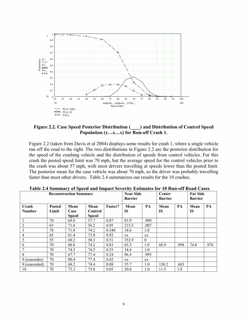
Figure 2.2. Case Speed Posterior Distribution (____) and Distribution of Control Speed

Population (x…x…x) for Run-off Crash 1. Figure 2.2 (taken from Davis et al 2004) displays some results for crash 1, where a single vehicle ran off the road to the right. The two distributions in Figure 2.2 are the posterior distribution for the speed of the crashing vehicle and the distribution of speeds from control vehicles. For this crash the posted speed limit was 70 mph, but the average speed for the control vehicles prior to the crash was about 57 mph, with most drivers travelling at speeds lower than the posted limit. The posterior mean for the case vehicle was about 70 mph, so the driver was probably travelling faster than most other drivers. Table 2.4 summarizes our results for the 10 crashes. Table 2.4 Summary of Speed and Impact Severity Estimates for 10 Run-off Road Cases

Reconstruction Summary Near Side Barrier

Center Barrier

Far Side Barrier

Crash Number

Posted Limit

Mean Case Speed

Mean Control Speed

Faster? Mean IS

PA Mean IS

PA Mean IS

PA

1 70 69.8 57.7 0.87 85.9 .999 2 65 71.0 56.2 0.95 215.3 .007 3 70 71.4 74.2 0.340 18.6 1.0 4 65 81.4 73.0 0.92 xx xx 5 55 69.2 58.3 0.51 352.9 0 6 70 80.8 74.2 0.83 65.5 1.0 68.9 .998 74.8 .976 7 70 74.5 74.5 0.55 34.4 1.0 8 70 67.7 77.4 0.24 96.4 .995 9 (rearender) 70 80.4 77.4 0.82 xx xx 9 (rearended) 70 68.2 74.4 0.08 55.7 1.0 130.2 .683 10 70 73.3 75.8 0.05 20.8 1.0 11.5 1.0

20 25 30 35 40 45 50 55 60 65 70 75 80 85 90 95 1000

0.1

0.2

0.3

0.4

0.5

0.6

0.7

0.8

0.9

1

P[v|y=1&e]P[v|y=0]PA[v]

Speed (mph)

Prob

abili

ties

1

0

p1 i

p2 i

PA j

10020 midpoint i midpoint i, PAint j,

10

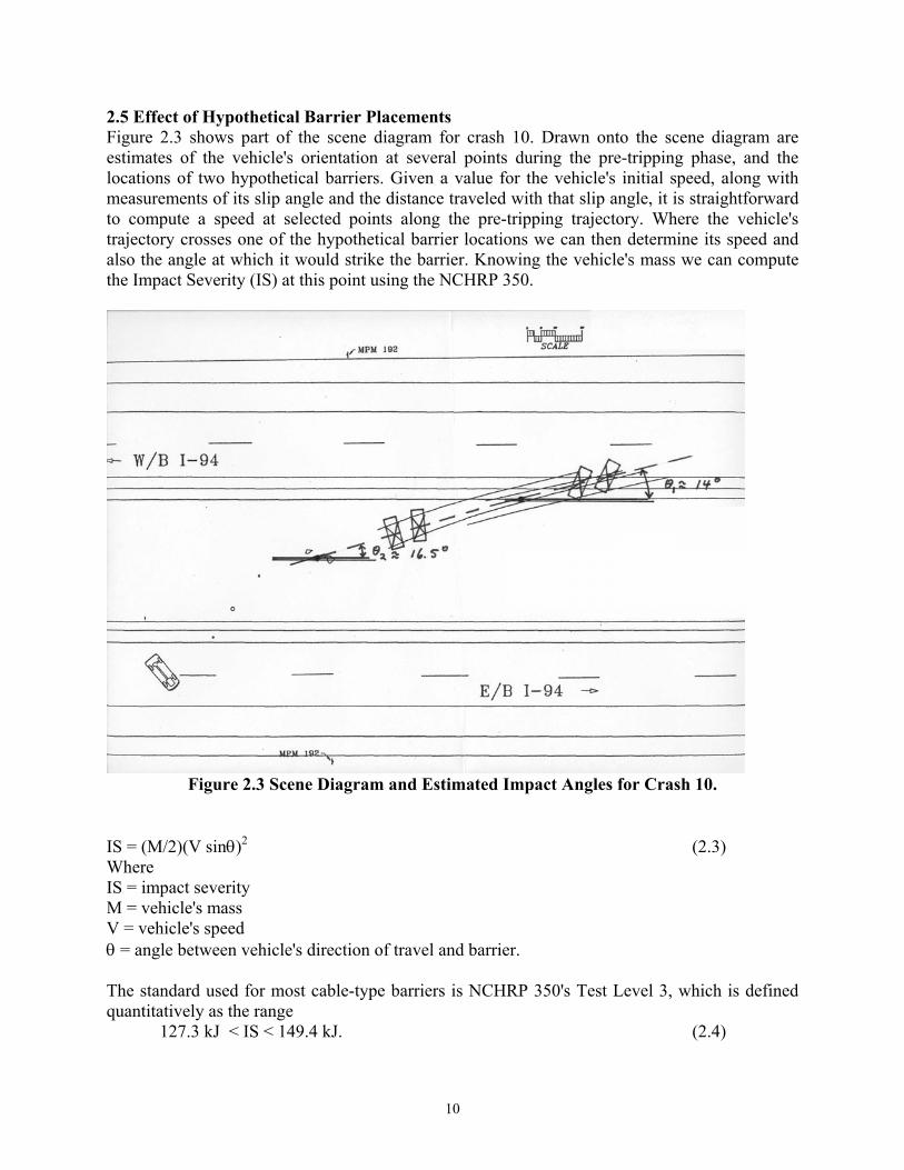
2.5 Effect of Hypothetical Barrier Placements Figure 2.3 shows part of the scene diagram for crash 10. Drawn onto the scene diagram are estimates of the vehicle's orientation at several points during the pre-tripping phase, and the locations of two hypothetical barriers. Given a value for the vehicle's initial speed, along with measurements of its slip angle and the distance traveled with that slip angle, it is straightforward to compute a speed at selected points along the pre-tripping trajectory. Where the vehicle's trajectory crosses one of the hypothetical barrier locations we can then determine its speed and also the angle at which it would strike the barrier. Knowing the vehicle's mass we can compute the Impact Severity (IS) at this point using the NCHRP 350.

Figure 2.3 Scene Diagram and Estimated Impact Angles for Crash 10.

IS = (M/2)(V sinθ)2 (2.3) Where IS = impact severity M = vehicle's mass V = vehicle's speed θ = angle between vehicle's direction of travel and barrier. The standard used for most cable-type barriers is NCHRP 350's Test Level 3, which is defined quantitatively as the range 127.3 kJ < IS < 149.4 kJ. (2.4)

11

To simulate the outcome of barrier collision we took each element of a Monte Carlo sample of the posterior distribution of the collision variables and then computed forward along the vehicle's pre-tripping trajectory to determine its speed and orientation at the hypothetical barrier placements. The simulated impact severity was then computed using equation (2.3). To allow for the fact that we may be uncertain as to the actual standard achieved by a given barrier, the simulated IS was compared to a random draw from a uniform distribution over the range [127.3 kJ, 149.4 kJ]. If the computed IS was less than the value of the random draw we recorded that the barrier stopped the vehicle, otherwise we recorded that it did not. The fraction of instances where the barrier stopped a vehicle then gave us an estimate of the probability of avoidance associated with the barrier placement. Since we had no plausible method for determining a vehicle's orientation after it tripped hypothetical impact severity was computed only for barrier encounters during the pre-tripping phase. For nine of the crashes it was possible to compute an IS for a barrier encountered just after the vehicle leaves the pavement (Near Side), for three of these it was also possible to compute an IS for a barrier encountered in the center of the median (Center). For one it was also possible to compute an IS for a barrier encountered at the pavement edge after traversing the median (Far Side). Table 2.4 summarizes these results as well. Looking at the first row of Table 2.4, we can see that for the first crash the posted speed limit was 70 mph and the best estimate of the crash vehicle's initial speed was 69.8 mph. The mean speed for other vehicles using that roadway at about the same time was only 57.7 mph, probably because of the snowy conditions. For a hypothetical barrier at the pavement edge the mean estimated impact severity was 85.9 kJ and the probability that the impact severity would not have exceeded NCHRP 350's Test Level 3 is 0.999. Since the vehicle ran off the road to the right, center median and far-side barrier placements were not relevant. Crash 2 also involved running off to the right in snowy conditions, but in this case the estimated impact severity was much higher, and the probability that a nearside barrier would have stopped the vehicle was only about .007. Although the vehicle in crash 2 was slightly heavier than that in crash 1, the main difference in their outcomes appears due to the estimated impact angles, about 19 degrees for crash 1 and about 30 degrees for crash 2. For crash 4 the vehicle's initial speed was estimated using the critical speed formula and a measured yaw mark radius so no pre-tripping trajectory and orientation was available. For crash 5, where an out-of-control vehicle left a county highway and collided on an adjacent freeway, the IS was computed at the location of an existing fence separating the county road from the freeway. Since the vehicle struck this fence at about a 56o angle, a Test Level 3 barrier at this same location would probably not have stopped the vehicle. For the remaining crashes there appears to be good reason to accept that a Test Level 3 barrier would have stopped the crashing vehicles before they reached their tripping points. 2.6 Discussion In this chapter we first reviewed briefly how Pearl's work on probabilistic causal models could be used in crash reconstruction to estimate important variables and test for causal factors, despite substantial, unavoidable uncertainties. These methods were applied to 10 fatal run-off-road crashes from Minnesota to estimate initial speeds of the crashing vehicles, and to test if NCHRP 350 Test Level 3-compliant barriers could have restrained the crashing vehicles. In five of the ten crashes we found evidence that the speed of the crashing vehicle at the point it began making tire marks was higher than that of other vehicles using the same road under similar conditions. In

12

seven of the ten crashes our analysis indicates that barriers would probably have restrained the crashing vehicles. Table 2.5 summarizes our results together with some other information gleaned from the crash investigations. The "Precipitating Event" column in Table 2.5 identifies actions or events preceding the driver's loss of control, as described by witnesses and/or survivors, and a variety of conditions appear. Crashes 1 and 2 both happened when snow made for a slippery roadway, where most drivers were travelling at speeds significantly below the posted limit, but where the crashing drivers appeared to be travelling nearer the posted limit. Crash 3 apparently started when the driver swerved to avoid a slower vehicle, while in crashes 4 and 5 it was not clear why the driver lost control. Crash 6 was precipitated by a road-rage type encounter, crash 7 by an encounter with a deer and crash 8 when an inexperienced driver was cut off by a merging vehicle. Crash 9 apparently happened when a speeding driver was unable to avoid clipping the rear of a vehicle travelling near the posted speed limit, and crash 10 resulted when the driver turned to back seat to interact with a crying child. In eight of these crashes the fatal victim was a driver and in two a passenger was killed. In contrast to the variety among the precipitating events, when we look at the "Seat Belt" and "Ejected" columns we see consistency. Eight of the ten fatalities were either not wearing their seat belts or, in the case of crash 10, had unfastened the lap belt. The fatal victim was ejected from the vehicle in seven of these eight cases. Table 2.5 Additional Summary of Ten Fatal Run-off Road Crashes Crash Precipitating Event Fatal Victim Barrier Effective? Seat Belt

Used? Ejected?

1 Snowy conditions/ Speed

Driver Yes No Yes

2 Snowy conditions/ Speed

Driver No No Yes

3 Evasive Action Driver Yes No Yes 4 "Sudden

Swerve"/Speed Driver Unknown No Yes

5 Unknown Driver No Uncertain No 6 Road Rage/Speed Passenger Yes No Yes 7 Deer Encounter Driver Yes No Yes 8 Inexperienced Driver

Cut Off Passenger Yes No Yes

9-1 Inattention/Speed Other Driver N/A N/A N/A 9-2 Rear ended Driver Yes Unknown No 10 Turn of child/backseat Driver Yes No lap belt No

13

CHAPTER THREE MEDIAN CROSSING CRASHES

3.1 Background In this chapter we will discuss reconstruction and causal analysis of median-crossing crashes. Our original intention in this project was to use the commercially available simulation program PC-CRASH as a model for linking crash input variables, such as a vehicle's initial speed and location and the driver's steering and braking inputs, to the vehicle trajectories obtained from crash-scene diagrams. This intention was based on a presentation made at the Fifth International Conference on Forensic Statistics, where an associate of the Netherlands Forensic Institute (NFI) described using PC-CRASH to compute Bayes estimates of vehicle speeds (Hoogstrate and Spek 2002). We obtained a license to use PC-CRASH in Spring 2003 but it was not until Spring 2004 that we were able to get details on the NFI's enhancements, and at this point it became apparent that these would not suit the needs of our project. As we have indicated in earlier chapters, in Bayesian analyses the posterior probability distribution for a variable characterizes what the available data tell us about that variable's probable values. To carry out a Bayesian analysis one must, at a minimum, be able to compute useful summaries of this distribution. For some problems this can be done analytically or by numerical integration, but for problems involving complex models or many variables Monte Carlo simulation is often the only practical alternative. The WinBUGS software used in Chapter Two accomplishes this, but is limited to fairly simple models. Although the NFI's enhancements to PC-CRASH could be used to estimate mean values from a posterior distribution they were not well-suited to computing probabilities of events, and in particular probabilities of avoidance. Without the source code for PC-CRASH we could not embed the model inside our own Monte Carlo routine, so we then coded our own vehicle trajectory simulator, BMS 1.0, based on the algorithm used by PC-CRASH (PC-CRASH 2001). Technical details of this simulator can be found in Pei (2004), and the model was coded using Microsoft Visual C++ 6.0. Numerous tests were conducted to compare the output from our simulator to that of PC-CRASH, under a variety of conditions. These included braking only with different braking intensities; steering only with different steering inputs; braking and steering with different combinations of braking intensity and steering input; acceleration only with different accelerations; and acceleration and steering with different combinations of acceleration and steering inputs. Different values for the initial speeds and different friction coefficients were also tested. The results produced by our simulator, under these various conditions, matched those of PC-CRASH. The next problem was to embed the trajectory simulation model inside a routine for generating Monte Carlo samples from the posterior distributions for our model's input variables. Although, as we have illustrated in the preceding chapter, Bayesian inference with simple crash models is readily accomplished using the WinBUGS software, at present the state of the art in Bayesian inference with complex simulation models is somewhat undeveloped (Poole and Raftery 2000). Development and coding of our own inference routine was thus unavoidable. As it turned out, special features of our crash data made this more straightforward than might have been expected, and we were able to use a method called Gibbs sampling to sample from the required posterior distributions. Section 3.2 describes Gibbs sampling and how we used it, and in section 3.3 we return to our work on median-crossing crashes. Section 3.4 contains a discussion of these results. Section 3.2 is somewhat technical and we have included it because this application of Gibbs sampling to a complex simulation model is one of the main accomplishment of this project. Readers who are mainly interested in our crash results can skip ahead to section 3.3. 3.2 Gibbs Sampling The Gibbs sampler dates back at least to Suomela (1976) in a Ph.D. thesis on Markov random fields. It was discovered independently by Creutz (1979), by Ripley (1979) and by Grenander (1983) and Geman and Geman (1984). The term “Gibbs sampler" is due to Geman and Geman (1984) and refers to the simulation of Gibbs distributions in statistical physics. The Gibbs sampler assumes that full conditional distributions are known and can be sampled. Informally speaking, the full conditional distribution for a variable is the probability distribution of that variable given that we know the values of all other model variables, along with our data measurements. The first step of the Gibbs sampler is to initialize all variables, and then, in the second step, new values for the variables are drawn one by one from the full conditional distributions, given the current values of all other variables. This new set of values then becomes the initial values and we return to the second step. This iterative process is repeated until a suitable sample size has been obtained. Under reasonably general conditions, the Gibbs sampler constructs a Markov Chain which has desired posterior distribution as its stationary distribution (Gilks et al., 1996). Two crucial issues then need to be resolved

14

when one wants to employ the Gibbs sampler. One is to identify the full conditional distributions, and the other is to generate samples from the full conditional distributions. First, let's denote the input variables for our model as ),..,( 1 nθθθ =

r, the output variables as ),..,( 1 pφφφ =

r,

and the relationship embedded in our model in which the values of output variables are determined by the values of the input variables as )(θφ

rrM= . The information available about the crash will be expressed as constraints on

the plausible values which output variables can assume. Generically we will denote this by saying that the output variable values must lie in a set X, or formally XM ∈)(θ

r. In all the crashes presented in this chapter the

constraints were obtained by determining simple upper and lower bounds on an output variable's values. For example, at a crash scene it may be possible to identify a skid mark but it is not clear where the skid mark actually began. This uncertainty can be expressed by identifying lower and upper bounds on the skid mark's length, so that estimates of the vehicle's initial speed must be consistent with skid mark lengths in that range. To implement the Gibbs sampler we need the full conditional distributions, which we will denote by

))(&|( XMii ∈− θθθπrr

, where i−θr

denotes the vector of input variables having element i deleted. By the definition of conditional probability, the full conditional distribution for variable θI is

∫ ∈

∈=∈−

in

nii dXM

XMXM

θθθθπθθθπ

θθθπ))(&,...,())(&,...,(

))(&|(1

1 r

rr

(3.1)

Letting

∈

∈=∈

falseisXMif

trueisXMifXMI

)(0

)(1])([

θ

θθ r

rr

(3.2)

denote the function which indicates whether or not our output constraints are satisfied, Equation 3.1 can be re-written as

∫ ∈∈

=∈−in

nii dXMI

XMIXMθθθθπ

θθθπθθθπ])([),...,(])([),...,())(&|(

1

1 r

rr

(3.3)

Then by assuming that our prior distributions for the input variables are independent, so that

)(),..,( 1 iin θπθθπ ∏= (3.4) we have

∫ ∈∈

=∈−iii

iiii dXMI

XMIXMθθθπ

θθπθθθπ])([)(])([)())(&|( r

rr

(3.5)

The full conditional distributions are thus simply truncated distributions of our priors.. Since Devroye (1986) has shown that samples from a truncated distribution can be obtained by first drawing samples from the non-truncated distribution and then selecting the suitable samples meeting the truncation constraints, as long as we can sample from the individual prior distributions we have what we need to implement the Gibbs sampler. Our method can be illustrated through a simple skid-mark example. Suppose a vehicle was traveling at speed V when the driver suddenly applied full braking. Assume that the prior distributions of the speed V and road friction coefficient µ are uniform distributions. That is

15

)(),(~)(),(~

221

121

µπµµµπ

==

uniformVVVuniformV

(3.6)

The length of the skid mark d is measured, but due to measurement error and other uncertainties existing at the scene, we can only determine a possible range, say between 1d and 2d , for the skid-mark length. The model relating the input variables, speed and friction coefficient to the output variable, skid mark length, is given by the standard braking formula

gVVMdµ

µ2

),(2

== (3.7)

The full conditional distributions for V and µ satisfy

]2

[)(),|(

]2

[)()),|(

22

1221

22

1121

dg

VdIdddV

dg

VdIVdddV

≤≤∝≤≤

≤≤∝≤≤

µµπµπ

µπµπ

(3.8)

The Gibbs sampler can then be implemented as follows: 1. Set initial values )',( )0()0()0( µθ V= and initialize the iteration counter of the chain 1=j .

2. Obtain a new value )',( )()()( jjj V µθ = from )1( −jθ through successive generation of values using the distributions in equation (3.8). The new value of )',( )()()( jjj V µθ = can be obtained by rejection sampling. Take )( jV for instance. A random

value is drawn from the uniform prior distribution of speed, )(1 Vπ , and the following constraint is checked

2)1(

2

1 2d

gVd j ≤≤ −µ

(3.9)

If the constraint is met, then current random value for speed is accepted as )( jV , otherwise, another random draw has to be carried out. 3. Change counter from j to 1+j , and return to step 2 until desired sample size is obtained. 3.3 Reconstruction of Median-Crossing Crashes Out of the crashes in our initial sample, seven involved median crossing and subsequent collision with an opposite-traveling vehicle. For one of these, the scene diagram and investigation report provided no information on the vehicle trajectories prior to collision. The major objective of simulating a median-crossing crash is to reproduce the pre-crash trajectory of the median-crossing vehicle. Several unknowns with regard to the inputs of the deterministic model exist in the pre-crash phase. These include the location and speed when the driver made the initial steering movement, whether or not the driver applied the brakes, and the friction coefficients of the road and median surfaces. For the remaining six crashes our first step was to use PC-CRASH to carry out a deterministic reconstruction of each. By this we mean a trial-and-error search for a combination of input variables that approximately reproduced the trajectories in the scene diagrams. For one of these, neither our homegrown software nor PC-CRASH could reproduce the tire trajectory recorded for the crash scene, which suggests that the information about the crash may have been inconsistent. For each of the remaining five it was possible to identify a plausible combination of input variable values consistent with the scene information. This does not mean that the sets of values identified in this step were the only, or even the best, ones consistent with the scene, and the goal of a Bayesian analysis is to identify the degree of probability attached to these input values.

16

3.3.1 Setting Up the Reconstructions Making the reconstruction problem even more complex are uncertainties concerning whether the steering input changed or whether the braking intensity changed over the course of the vehicle's trajectory. Field research suggests that drivers tend to lose control of the vehicle once yawing begins, in which case the input would not change the vehicle’s path after the beginning of the yaw (Viano and Parenteau, 2003). This hypothesis was further tested in PC-CRASH. After yawing begins, the simulated trajectory does not change despite changes in steering. Also, replacing an unknown sequence of braking intensities during the pre-crash phase with an average braking intensity should give a reasonable approximation. In our reconstructions we assumed a constant steering input, and a constant braking intensity once the driver begins braking, hold during pre-crash phase. Another assumption we made was that the surface over which a vehicle crosses was essentially flat. None of the crash reports indicated that collisions occurred on roadways with pronounced up or downgrades, and the angles at which the vehicles traversed the medians tended to range between 15 degrees and 39 degrees with respect to the roadway, with 20o being a typical value. We can get a rough idea of the effect of our simplifying assumption by applying a simple skidding model to the case of vehicle traversing a median with a cross-slope of 1:4 at an angle of 25 degrees. The vehicle's initial speed is assumed to be 88 feet/sec (60 mph), the median is assumed to be 60 feet wide, and the combination of braking and friction has the vehicle decelerating at 0.4g. If we ignore the median's cross-slope and model the trajectory as occurring on a flat surface the vehicle's speed when it reaches the center of the median will be about 77 fps and when it reaches the far side of the median the speed will be about 64 fps. Now, allowing for the effect of the median's cross slope, the downgrade along the path of the vehicle is about 10.5%, so the speed of the vehicle when it crosses the center of the median will now be about 80 fps, but when it reaches the far side of the median it will again be about 64 fps. This example indicates that by treating the medians as flat our estimates of speed and impact severity at the near and far sides of the median should be mainly unaffected, while estimates for the center will be slightly low. An important issue with regard to the outputs of our model is to determine criteria for identifying when the simulated trajectory matches the scene trajectory. Obviously, it is not practical to compare all points in the trajectory, and what we did was select several points (called diagnostic points) located evenly along the trajectory path, and make comparisons at these points regarding the vehicle’s location, orientation, and speed (if corresponding scene speed was known). If all simulated diagnostic points were within a specified distance from the corresponding scene points, it was concluded that the scene trajectory was reproduced. Tolerances of 1 meter in the X direction, 0.5 meter in the Y direction, and 10 degrees in vehicle orientation were typical values used in our study. If the simulated center of gravity of the vehicle along its traveled path was contained in these ranges, the simulation run and the input values were accepted by our Gibbs sampler. For the diagnostic points where scene speed was known, the ranges of the scene speed were used as the constraint for simulated speed at the corresponding places. Since a Cartesian coordinate system was used in our model, the model’s input variables reduce to the vehicle’s initial X and Y coordinates, the vehicle’s initial speed in the X and Y directions, the driver’s initial steering input, the driver’s reaction time to brake, the driver’s average braking intensity, and the friction coefficients for the road surface and the median surface. Selection of prior probability distributions for these input variables was less clear. The strategy we used was to identify priors that appeared to be consistent with current practice. It is often possible to dig out defensible prior ranges for input variables in deterministic sensitivity analyses (Niederer 1991), and Wood and O’Riordain (1994) have argued that, in the absence of more specific information, uniform distributions restricted to these ranges offer a plausible extension of the deterministic sensitivity methods. Following these suggestions, uniform prior distributions were used for the input variables. For the initial location of the vehicle in the X direction, often one bound can be easily identified based on the start of tire marks in the scene diagram, but the other bound for this prior distribution is unknown. Our practice was to choose a value large enough so that reasonable values of initial X location were included in the prior range. The initial Y coordinates of the vehicle were bounded by the edges of the road and were easily identified. Similar to the initial X location, the range of the initial speed in the X direction was unknown and a wide enough range was picked so that all reasonable values were included. The lateral initial speed tends to be minimal under normal driving situations, and the range [-1 m/s, 1m/s] should take all reasonable possibilities into account. As to the initial steering input, Mazzae et al. (1999) conducted research on driver crash-avoidance behavior, and based on their study we selected a range of [0 degree, 110 degrees] . The range for the reaction time to brake was chosen to be [0.5 seconds, 2.5 seconds], which covers the values obtained by Fambro et al. (1998) in surprise braking tests, and the midpoint of which (1.5 seconds) equals a popular default value (Stewart-Morris, 1995). The range for the friction coefficient of road surface depended on the

17

surface conditions. Concrete surfaces have different ranges than do asphalt road surfaces, and dry surfaces have different ranges than wet surfaces. The ranges we chose were primarily taken from Fricke (1990, p. 62-14). For example, for a dry traveled asphalt pavement, the range [0.55, 0.90] is chosen, where 0.55 corresponds to the lower bound for a dry, traveled asphalt pavement and 0.9 is what Fricke considers a reasonable upper bound for most cases(1990, p. 62-13). The ranges for the friction coefficient of the median were also based on Fricke (1990, p. 62-14), with some exceptions. There are no ranges pointed out by Fricke for grass surface under various conditions. The average value for dry grass suggested by Warner et al. (1983) was 0.5g, while Limpert (1989) claimed that 0.35 could be used for dry grass. So for dry grass, a range of [0.35, 0.55] was picked. For wet grass surface, the range [0.15, 0.35] was chosen in our study. 3.3.2 Actual Reconstructions Crash One Figure 3.1 depicts the after-crash situation information for Crash One. The units of the X and Y coordinates are in meters.

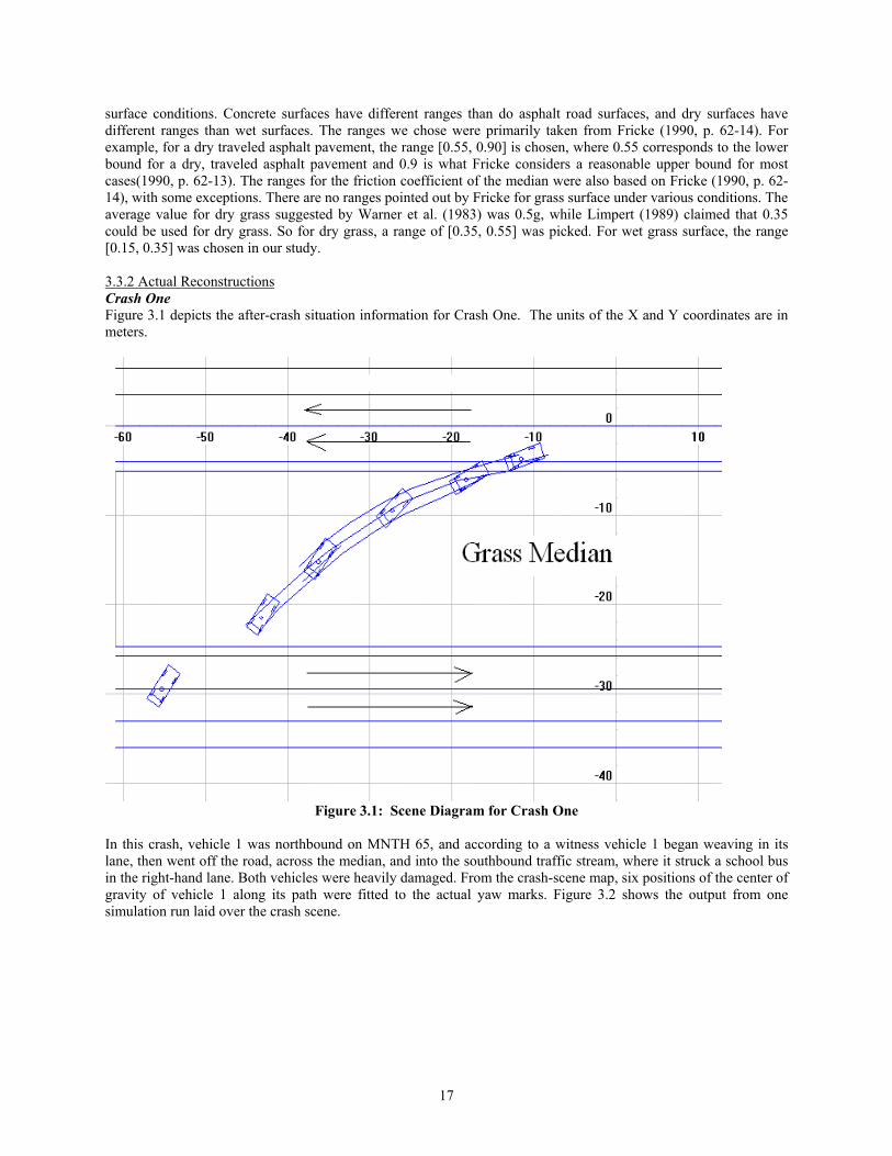
Figure 3.1: Scene Diagram for Crash One

In this crash, vehicle 1 was northbound on MNTH 65, and according to a witness vehicle 1 began weaving in its lane, then went off the road, across the median, and into the southbound traffic stream, where it struck a school bus in the right-hand lane. Both vehicles were heavily damaged. From the crash-scene map, six positions of the center of gravity of vehicle 1 along its path were fitted to the actual yaw marks. Figure 3.2 shows the output from one simulation run laid over the crash scene.

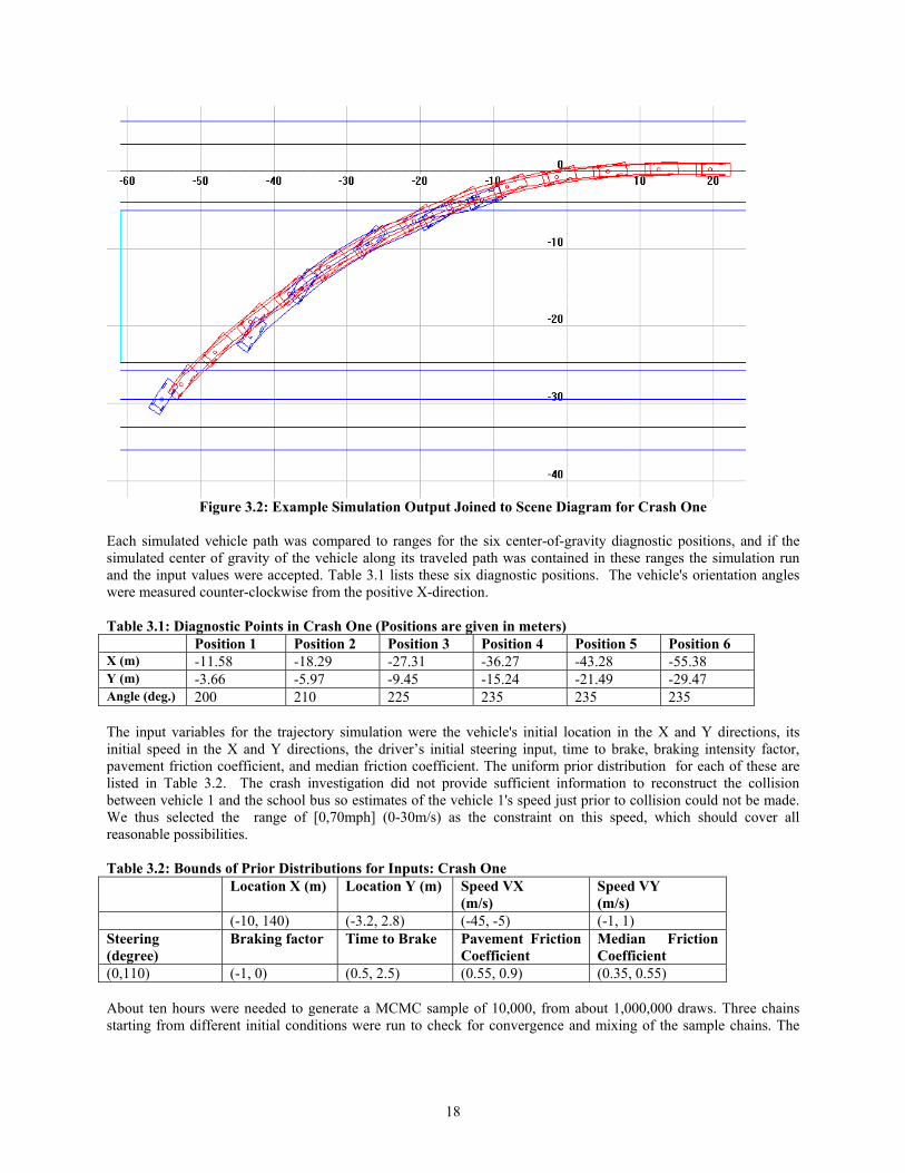
18

Figure 3.2: Example Simulation Output Joined to Scene Diagram for Crash One

Each simulated vehicle path was compared to ranges for the six center-of-gravity diagnostic positions, and if the simulated center of gravity of the vehicle along its traveled path was contained in these ranges the simulation run and the input values were accepted. Table 3.1 lists these six diagnostic positions. The vehicle's orientation angles were measured counter-clockwise from the positive X-direction. Table 3.1: Diagnostic Points in Crash One (Positions are given in meters) Position 1 Position 2 Position 3 Position 4 Position 5 Position 6 X (m) -11.58 -18.29 -27.31 -36.27 -43.28 -55.38 Y (m) -3.66 -5.97 -9.45 -15.24 -21.49 -29.47 Angle (deg.) 200 210 225 235 235 235

The input variables for the trajectory simulation were the vehicle's initial location in the X and Y directions, its initial speed in the X and Y directions, the driver’s initial steering input, time to brake, braking intensity factor, pavement friction coefficient, and median friction coefficient. The uniform prior distribution for each of these are listed in Table 3.2. The crash investigation did not provide sufficient information to reconstruct the collision between vehicle 1 and the school bus so estimates of the vehicle 1's speed just prior to collision could not be made. We thus selected the range of [0,70mph] (0-30m/s) as the constraint on this speed, which should cover all reasonable possibilities. Table 3.2: Bounds of Prior Distributions for Inputs: Crash One Location X (m) Location Y (m) Speed VX

(m/s) Speed VY (m/s)

(-10, 140) (-3.2, 2.8) (-45, -5) (-1, 1) Steering (degree)

Braking factor Time to Brake Pavement Friction Coefficient

Median Friction Coefficient

(0,110) (-1, 0) (0.5, 2.5) (0.55, 0.9) (0.35, 0.55) About ten hours were needed to generate a MCMC sample of 10,000, from about 1,000,000 draws. Three chains starting from different initial conditions were run to check for convergence and mixing of the sample chains. The

19

Gelman-Rubin test was used to assess the extent to which the three chains tended to cover the same region of the space of possible input variable values, and the results of these tests are displayed in Table 3.3. Table 3.3 Gelman and Rubin Statistics for Crash One

VARIABLE Point est. 97.5% quantile InitPosX 1.04 1.14 InitPosY 1.04 1.13 BrakeFactor 1.00 1.00 SpeedAtX 1.03 1.08 SpeedAtY 1.00 1.00 Braketime 1.00 1.00 RoadFric 1.00 1.01 GrassFri 1.00 1.01 SterFactor 1.00 1.01

Gelman and Rubin (Gilks, et al., 1996) suggested that if the values in the “point estimation” column were all less than 1.1 and the values in “97.5% quantile” column were all less than 1.2, reasonably good convergence was reached. The values of the Gelman-Rubin statistics in Table 3.3 were consistent with converged chains, indicating that feasible region of initial inputs ought to be connected. Estimates computed separately for each chain showed little across-chain differences. Finally, the three chains were then combined to produce the final estimates. The posterior range, mean and standard deviation of each input variables is shown in Table 3.4. Table 3.4 Statistics of Posterior Distributions for Inputs in Crash One Variables Location X

(m) Location Y (m)

Speed VX (m/s)

Speed VY (m/s)

Range (-2.7, 20.8) (-3.2, 1.6) (-26.5,-14.7) (-1, 1) Mean(Std.) 3.00(5.19) -1.67(1.07) -20.20(2.12) 0 (0.41) Variables Steering

(degree) Braking factor

Time to Brake

Pavement Friction Coefficient

Median Friction Coefficient

Range (51,110) (-1, 0) (1.75, 2.45) (0.55, 0.9) (0.35, 0.55) Mean(Std.) 88.74 (13.2) -0.5(0.29) 2.27(0.15) 0.72(0.10) 0.47(0.06)

Figure 3.3 shows the prior and posterior distributions for vehicle 1's initial speed. As was the case for the crashes discussed in Chapter Two, data were available on the speeds of vehicles using the same roadway under conditions similar to those when the crash occurred, and for Crash One these data were collected by a nearby automatic traffic recorder (ATR). The distribution of these speeds is also shown in Figure 3.3.

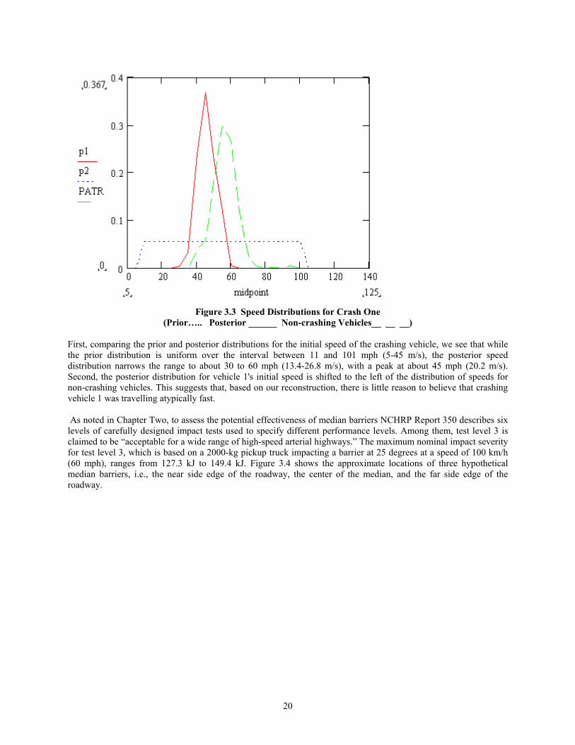
20

Figure 3.3 Speed Distributions for Crash One

(Prior….. Posterior ______ Non-crashing Vehicles__ __ __)

First, comparing the prior and posterior distributions for the initial speed of the crashing vehicle, we see that while the prior distribution is uniform over the interval between 11 and 101 mph (5-45 m/s), the posterior speed distribution narrows the range to about 30 to 60 mph (13.4-26.8 m/s), with a peak at about 45 mph (20.2 m/s). Second, the posterior distribution for vehicle 1's initial speed is shifted to the left of the distribution of speeds for non-crashing vehicles. This suggests that, based on our reconstruction, there is little reason to believe that crashing vehicle 1 was travelling atypically fast. As noted in Chapter Two, to assess the potential effectiveness of median barriers NCHRP Report 350 describes six levels of carefully designed impact tests used to specify different performance levels. Among them, test level 3 is claimed to be “acceptable for a wide range of high-speed arterial highways.” The maximum nominal impact severity for test level 3, which is based on a 2000-kg pickup truck impacting a barrier at 25 degrees at a speed of 100 km/h (60 mph), ranges from 127.3 kJ to 149.4 kJ. Figure 3.4 shows the approximate locations of three hypothetical median barriers, i.e., the near side edge of the roadway, the center of the median, and the far side edge of the roadway.

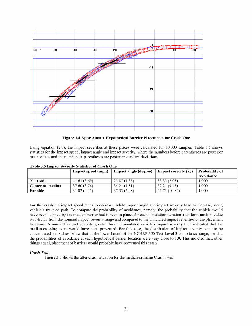
21

Figure 3.4 Approximate Hypothetical Barrier Placements for Crash One

Using equation (2.3), the impact severities at these places were calculated for 30,000 samples. Table 3.5 shows statistics for the impact speed, impact angle and impact severity, where the numbers before parentheses are posterior mean values and the numbers in parentheses are posterior standard deviations. Table 3.5 Impact Severity Statistics of Crash One Impact speed (mph) Impact angle (degree) Impact severity (kJ) Probability of

Avoidance Near side 41.61 (3.69) 23.87 (1.35) 33.33 (7.03) 1.000 Center of median 37.60 (3.76) 34.21 (1.81) 52.21 (9.45) 1.000 Far side 31.02 (4.45) 37.33 (2.08) 41.73 (10.84) 1.000 For this crash the impact speed tends to decrease, while impact angle and impact severity tend to increase, along vehicle’s traveled path. To compute the probability of avoidance, namely, the probability that the vehicle would have been stopped by the median barrier had it been in place, for each simulation iteration a uniform random value was drawn from the nominal impact severity range and compared to the simulated impact severities at the placement locations. A nominal impact severity greater than the simulated vehicle's impact severity then indicated that the median-crossing event would have been prevented. For this case, the distribution of impact severity tends to be concentrated on values below that of the lower bound of the NCHRP 350 Test Level 3 compliance range, so that the probabilities of avoidance at each hypothetical barrier location were very close to 1.0. This indicted that, other things equal, placement of barriers would probably have prevented this crash. Crash Two

Figure 3.5 shows the after-crash situation for the median-crossing Crash Two.

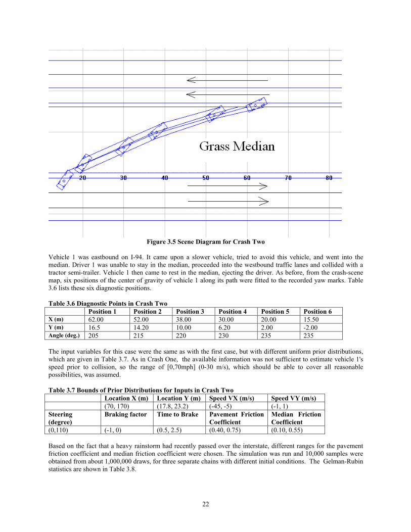
22

Figure 3.5 Scene Diagram for Crash Two

Vehicle 1 was eastbound on I-94. It came upon a slower vehicle, tried to avoid this vehicle, and went into the median. Driver 1 was unable to stay in the median, proceeded into the westbound traffic lanes and collided with a tractor semi-trailer. Vehicle 1 then came to rest in the median, ejecting the driver. As before, from the crash-scene map, six positions of the center of gravity of vehicle 1 along its path were fitted to the recorded yaw marks. Table 3.6 lists these six diagnostic positions. Table 3.6 Diagnostic Points in Crash Two Position 1 Position 2 Position 3 Position 4 Position 5 Position 6 X (m) 62.00 52.00 38.00 30.00 20.00 15.50 Y (m) 16.5 14.20 10.00 6.20 2.00 -2.00 Angle (deg.) 205 215 220 230 235 235 The input variables for this case were the same as with the first case, but with different uniform prior distributions, which are given in Table 3.7. As in Crash One, the available information was not sufficient to estimate vehicle 1's speed prior to collision, so the range of [0,70mph] (0-30 m/s), which should be able to cover all reasonable possibilities, was assumed. Table 3.7 Bounds of Prior Distributions for Inputs in Crash Two Location X (m) Location Y (m) Speed VX (m/s) Speed VY (m/s) (70, 170) (17.8, 23.2) (-45, -5) (-1, 1) Steering (degree)

Braking factor Time to Brake Pavement Friction Coefficient

Median Friction Coefficient

(0,110) (-1, 0) (0.5, 2.5) (0.40, 0.75) (0.10, 0.55)

Based on the fact that a heavy rainstorm had recently passed over the interstate, different ranges for the pavement friction coefficient and median friction coefficient were chosen. The simulation was run and 10,000 samples were obtained from about 1,000,000 draws, for three separate chains with different initial conditions. The Gelman-Rubin statistics are shown in Table 3.8.

23

Table 3.8 Gelman-Rubin Statistics for Crash Two VARIABLE Point est. 97.5% quantile InitPosX 1.01 1.02 InitPosY 1.01 1.03 BrakeFactor 1.00 1.00 SpeedAtX 1.04 1.13 SpeedAtY 1.00 1.01 Braketime 1.01 1.01 RoadFric 1.05 1.16 GrassFri 1.00 1.02 SterFactor 1.00 1.00

The posterior range, mean and standard deviation of each input variable are shown in Table 3.9. Table 3.9 Statistics of Posterior Distributions for Inputs in Crash Two Variables Location X

(m) Location Y (m)

Speed VX (m/s)

Speed VY (m/s)

Range (73, 102) (17.8, 20.9) (-30.2,-17.7) (-1, 1) Mean(Std.) 87.2(6.31) 18.59(0.63) -24.79(2.56) -0.12 (0.56) Variables Steering

(degree) Braking factor

Time to Brake

Pavement Friction Coefficient

Median Friction Coefficient

Range (40,110) (-1, 0) (1.65, 2.45) (0.4, 0.75) (0.20, 0.55) Mean(Std.) 74.8(17.28) -0.5(0.29) 2.28(0.16) 0.61(0.09) 0.44(0.08)

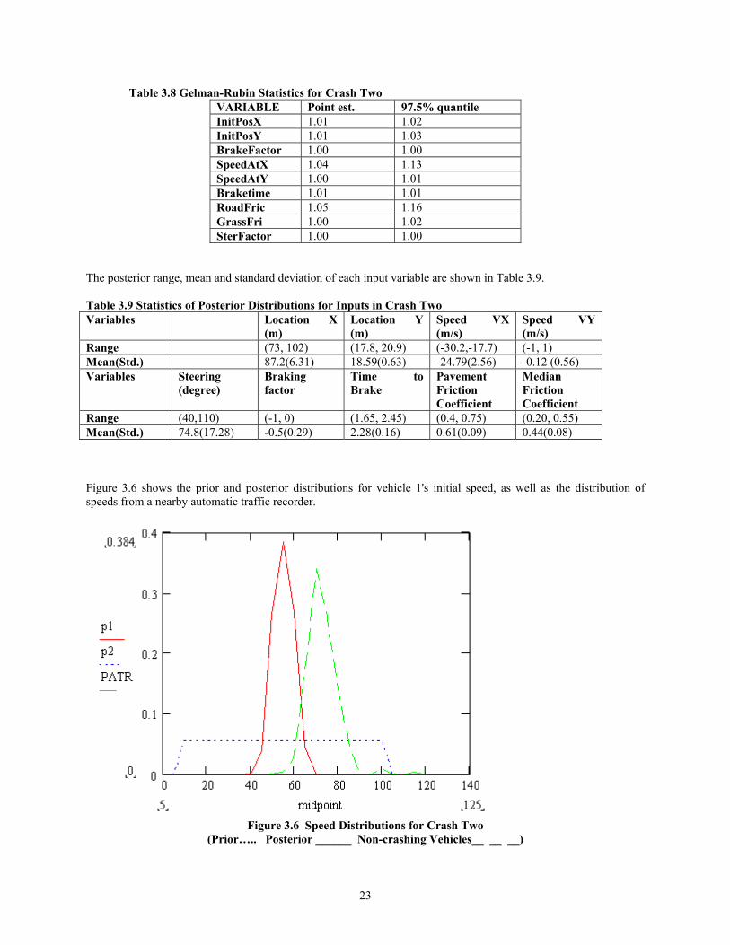
Figure 3.6 shows the prior and posterior distributions for vehicle 1's initial speed, as well as the distribution of speeds from a nearby automatic traffic recorder.

Figure 3.6 Speed Distributions for Crash Two

(Prior….. Posterior ______ Non-crashing Vehicles__ __ __)

24

The dotted curve shows the prior distribution of vehicle 1's initial speed, uniform over the range of 11 to 101 mph (5-45m/s). The posterior speed distribution narrows the range down to about 40 to 65 mph (18-29 m/s) with a peak of approximately 55 mph (20.8 m/s), indicating that our results were informative about vehicle 1's initial speed. As can be seen, vehicle 1 did not appear to be traveling at a high speed compared to other roadway users. Table 3.10 shows statistics about the impact speed, impact angle and impact severity, where the numbers before parentheses are mean values and the numbers in parentheses are standard deviations. Table 3.10 Impact Severity Statistics for Crash Two Impact speed (mph) Impact angle

(degrees) Impact severity (kJ) Probability of

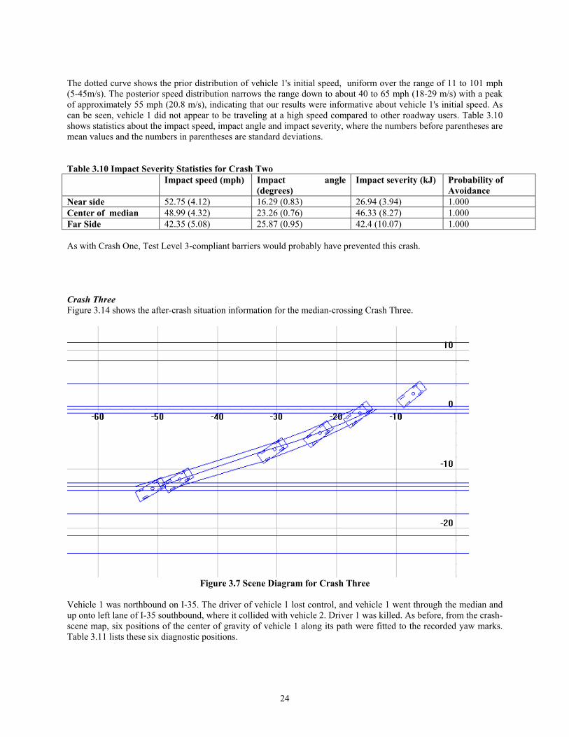
Avoidance Near side 52.75 (4.12) 16.29 (0.83) 26.94 (3.94) 1.000 Center of median 48.99 (4.32) 23.26 (0.76) 46.33 (8.27) 1.000 Far Side 42.35 (5.08) 25.87 (0.95) 42.4 (10.07) 1.000 As with Crash One, Test Level 3-compliant barriers would probably have prevented this crash. Crash Three Figure 3.14 shows the after-crash situation information for the median-crossing Crash Three.

Figure 3.7 Scene Diagram for Crash Three

Vehicle 1 was northbound on I-35. The driver of vehicle 1 lost control, and vehicle 1 went through the median and up onto left lane of I-35 southbound, where it collided with vehicle 2. Driver 1 was killed. As before, from the crash-scene map, six positions of the center of gravity of vehicle 1 along its path were fitted to the recorded yaw marks. Table 3.11 lists these six diagnostic positions.

25

Table 3.11 Diagnostic Points for Crash Three Position 1 Position 2 Position 3 Position 4 Position 5 Position 6 X (m) -50.90 -46.33 -30.48 -22.86 -16.15 -7.19 Y (m) -13.29 -11.77 -6.71 -3.96 -0.61 2.71 Angle (deg.) 30 32 35 40 40 40 The input variables for this case were the same as with the first two cases, but with different uniform prior distributions, which are given in Table 3.12. Insufficient information made it impossible for us to reconstruct the collision between vehicles 1 and 2, so as before a range of [0,70mph] (0-30 m/s) was assumed for the pre-impact speed.

Table 3.12 Bounds of Prior Distributions for Inputs in Crash Three Location X (m) Location Y (m) Speed VX (m/s) Speed VY (m/s) (-200, -60) (-20.4, -14.4) (5, 45) (-1, 1) Steering (degree)

Braking factor Time to Brake Pavement Friction Coefficient

Median Friction Coefficient

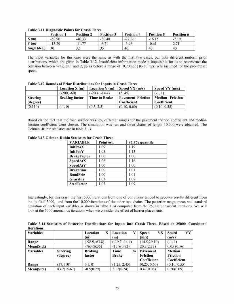
(0,110) (-1, 0) (0.5, 2.5) (0.10, 0.60) (0.10, 0.55)

Based on the fact that the road surface was icy, different ranges for the pavement friction coefficient and median friction coefficient were chosen. The simulation was run and three chains of length 10,000 were obtained. The Gelman -Rubin statistics are in table 3.13. Table 3.13 Gelman-Rubin Statistics for Crash Three

VARIABLE Point est. 97.5% quantile InitPosX 1.09 1.19 InitPosY 1.05 1.13 BrakeFactor 1.00 1.00 SpeedAtX 1.06 1.16 SpeedAtY 1.00 1.00 Braketime 1.00 1.01 RoadFric 1.00 1.01 GrassFri 1.03 1.08 SterFactor 1.03 1.09

Interestingly, for this crash the first 5000 iterations from one of our chains tended to produce results different from the its final 5000, and from the 10,000 iterations of the other two chains. The posterior range, mean and standard deviation of each input variables is shown in table 3.14 computed from the 25,000 consistent iterations. We will look at the 5000 anomalous iterations when we consider the effect of barrier placements. Table 3.14 Statistics of Posterior Distributions for Inputs into Crash Three, Based on 25000 'Consistent' Iterations. Variables Location X

(m) Location Y (m)

Speed VX (m/s)

Speed VY (m/s)

Range (-98.9,-63.8) (-19.7,-14.4) (14.5,29.10) (-1, 1) Mean(Std.) -76.4(6.35) -15.8(0.92) 20.3(2.33) 0.05 (0.56) Variables Steering

(degree) Braking factor

Time to Brake

Pavement Friction Coefficient

Median Friction Coefficient

Range (37,110) (-1, 0) (1.25, 2.45) (0.25, 0.60) (0.10, 0.55) Mean(Std.) 83.7(15.67) -0.5(0.29) 2.17(0.24) 0.47(0.08) 0.20(0.09)

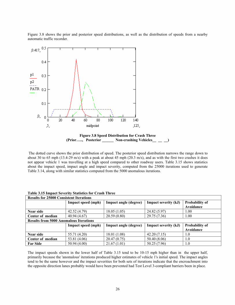
26

Figure 3.8 shows the prior and posterior speed distributions, as well as the distribution of speeds from a nearby automatic traffic recorder.

Figure 3.8 Speed Distribution for Crash Three

(Prior….., Posterior ______ Non-crashing Vehicles__ __ __)

The dotted curve shows the prior distribution of speed. The posterior speed distribution narrows the range down to about 30 to 65 mph (13.4-29 m/s) with a peak at about 45 mph (20.3 m/s), and as with the first two crashes it does not appear vehicle 1 was travelling at a high speed compared to other roadway users. Table 3.15 shows statistics about the impact speed, impact angle and impact severity, computed from the 25000 iterations used to generate Table 3.14, along with similar statistics computed from the 5000 anomalous iterations. Table 3.15 Impact Severity Statistics for Crash Three Results for 25000 Consistent Iterations Impact speed (mph) Impact angle (degree) Impact severity (kJ) Probability of

Avoidance Near side 42.52 (4.79) 18.05 (1.05) 24.82 (5.97) 1.00 Center of median 40.94 (4.67) 20.59 (0.80) 29.75 (7.36) 1.00 Results from 5000 Anomalous Iterations Impact speed (mph) Impact angle (degree) Impact severity (kJ) Probability of

Avoidance Near side 55.71 (4.20) 18.01 (1.08) 42.20 (7.15) 1.0 Center of median 53.81 (4.06) 20.47 (0.75) 50.40 (8.06) 1.0 Far Side 50.94 (4.00) 21.67 (1.01) 50.25 (7.96) 1.0 The impact speeds shown in the lower half of Table 3.15 tend to be 10-15 mph higher than in the upper half, primarily because the 'anomalous' iterations produced higher estimates of vehicle 1's initial speed. The impact angles tend to be the same however and the impact severities for both sets of iterations indicate that the encroachment into the opposite direction lanes probably would have been prevented had Test Level 3-compliant barriers been in place.

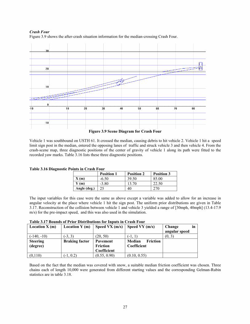
27

Crash Four Figure 3.9 shows the after-crash situation information for the median-crossing Crash Four.

Figure 3.9 Scene Diagram for Crash Four

Vehicle 1 was southbound on USTH 61. It crossed the median, causing debris to hit vehicle 2. Vehicle 1 hit a speed limit sign post in the median, entered the opposing lanes of traffic and struck vehicle 3 and then vehicle 4. From the crash-scene map, three diagnostic positions of the center of gravity of vehicle 1 along its path were fitted to the recorded yaw marks. Table 3.16 lists these three diagnostic positions. Table 3.16 Diagnostic Points in Crash Four

Position 1 Position 2 Position 3 X (m) -6.50 39.50 85.00 Y (m) -3.80 13.70 22.50 Angle (deg.) 25 40 270

The input variables for this case were the same as above except a variable was added to allow for an increase in angular velocity at the place where vehicle 1 hit the sign post. The uniform prior distributions are given in Table 3.17. Reconstruction of the collision between vehicle 1 and vehicle 3 yielded a range of [30mph, 40mph] (13.4-17.9 m/s) for the pre-impact speed, and this was also used in the simulation. Table 3.17 Bounds of Prior Distributions for Inputs in Crash Four Location X (m) Location Y (m) Speed VX (m/s) Speed VY (m/s) Change in

angular speed (-140, -10) (-3, 3) (20, 50) (-1, 1) (0, 3) Steering (degree)

Braking factor Pavement Friction Coefficient

Median Friction Coefficient

(0,110) (-1, 0.2) (0.55, 0.90) (0.10, 0.55) Based on the fact that the median was covered with snow, a suitable median friction coefficient was chosen. Three chains each of length 10,000 were generated from different starting values and the corresponding Gelman-Rubin statistics are in table 3.18.

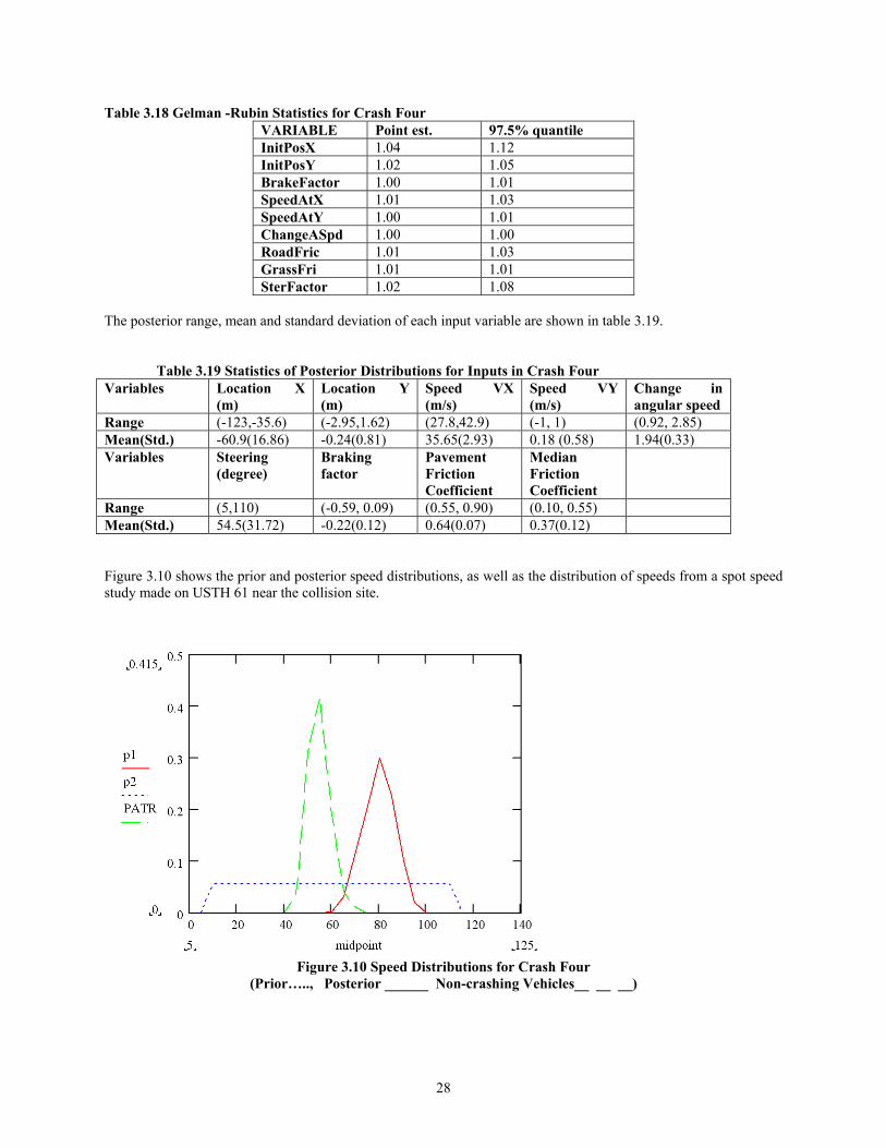
28

Table 3.18 Gelman -Rubin Statistics for Crash Four VARIABLE Point est. 97.5% quantile InitPosX 1.04 1.12 InitPosY 1.02 1.05 BrakeFactor 1.00 1.01 SpeedAtX 1.01 1.03 SpeedAtY 1.00 1.01 ChangeASpd 1.00 1.00 RoadFric 1.01 1.03 GrassFri 1.01 1.01 SterFactor 1.02 1.08

The posterior range, mean and standard deviation of each input variable are shown in table 3.19.

Table 3.19 Statistics of Posterior Distributions for Inputs in Crash Four

Variables Location X (m)

Location Y (m)

Speed VX (m/s)

Speed VY (m/s)

Change in angular speed

Range (-123,-35.6) (-2.95,1.62) (27.8,42.9) (-1, 1) (0.92, 2.85) Mean(Std.) -60.9(16.86) -0.24(0.81) 35.65(2.93) 0.18 (0.58) 1.94(0.33) Variables Steering

(degree) Braking factor

Pavement Friction Coefficient

Median Friction Coefficient

Range (5,110) (-0.59, 0.09) (0.55, 0.90) (0.10, 0.55) Mean(Std.) 54.5(31.72) -0.22(0.12) 0.64(0.07) 0.37(0.12)

Figure 3.10 shows the prior and posterior speed distributions, as well as the distribution of speeds from a spot speed study made on USTH 61 near the collision site.

Figure 3.10 Speed Distributions for Crash Four

(Prior….., Posterior ______ Non-crashing Vehicles__ __ __)

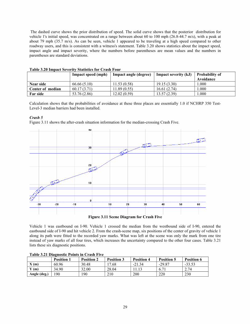
29

The dashed curve shows the prior distribution of speed. The solid curve shows that the posterior distribution for vehicle 1's initial speed, was concentrated on a range between about 60 to 100 mph (26.8-44.7 m/s), with a peak at about 79 mph (35.7 m/s). As can be seen, vehicle 1 appeared to be traveling at a high speed compared to other roadway users, and this is consistent with a witness's statement. Table 3.20 shows statistics about the impact speed, impact angle and impact severity, where the numbers before parentheses are mean values and the numbers in parentheses are standard deviations. Table 3.20 Impact Severity Statistics for Crash Four Impact speed (mph) Impact angle (degree) Impact severity (kJ) Probability of

Avoidance Near side 66.66 (5.10) 11.53 (0.58) 19.15 (3.30) 1.000 Center of median 60.17 (3.71) 11.89 (0.55) 16.61 (2.74) 1.000 Far side 53.76 (2.86) 12.02 (0.59) 13.57 (2.39) 1.000 Calculation shows that the probabilities of avoidance at these three places are essentially 1.0 if NCHRP 350 Test-Level-3 median barriers had been installed. Crash 5 Figure 3.11 shows the after-crash situation information for the median-crossing Crash Five.

Figure 3.11 Scene Diagram for Crash Five

Vehicle 1 was eastbound on I-90. Vehicle 1 crossed the median from the westbound side of I-90, entered the eastbound side of I-90 and hit vehicle 2. From the crash-scene map, six positions of the center of gravity of vehicle 1 along its path were fitted to the recorded yaw marks. What was left at the scene was only the mark from one tire instead of yaw marks of all four tires, which increases the uncertainty compared to the other four cases. Table 3.21 lists these six diagnostic positions. Table 3.21 Diagnostic Points in Crash Five Position 1 Position 2 Position 3 Position 4 Position 5 Position 6 X (m) 60.96 30.48 17.68 -21.34 -29.87 -33.53 Y (m) 34.90 32.00 28.04 11.13 6.71 2.74 Angle (deg.) 190 190 210 200 220 230

30

The input variables for this case were the same as with the first case, but with different uniform prior distributions, which are given in Table 3.22. Insufficient information made it impossible for us to reconstruct the collision between vehicles 1 and 2, so a range of [0,70mph] (0-30 m/s), was assumed for vehicle 1's pre-impact speed. Table 3.22 Bounds of Prior Distributions for Inputs in Crash Five Location X (m) Location Y (m) Speed VX (m/s) Speed VY (m/s) (60, 160) (35, 39) (-45, -5) (-1, 1) Steering (degree)

Braking factor Time to Brake Pavement Friction Coefficient

Median Friction Coefficient

(0,110) (-1, 0) (0.5, 2.5) (0.60, 0.90) (0.10, 0.55) The simulation was run and three chains of 10,000 samples were obtained. The Gelman-Rubin statistics are in Table 3.23. Table 3.23 Gelman-Rubin Statistics for Crash Five

VARIABLE Point est. 97.5% quantile InitPosX 1.01 1.02 InitPosY 1.00 1.00 BrakeFactor 1.00 1.00 SpeedAtX 1.00 1.00 SpeedAtY 1.00 1.00 Braketime 1.01 1.04 RoadFric 1.01 1.03 GrassFri 1.00 1.01 SteerFactor 1.01 1.03

The posterior range, mean and standard deviation of each input variables is shown in table 3.24.

Table 3.24 Statistics of Posterior Distributions for Inputs in Crash Five Variables Location X

(m) Location Y (m)

Speed VX (m/s)

Speed VY (m/s)

Range (61.2,80.1) (35,35.8) (-32.2,-21.5) (-1, 1) Mean(Std.) 67.68(3.69) 35.24(0.17) -28.2(1.50) -0.29(0.51) Variables Steering

(degree) Braking factor

Time to Brake

Pavement Friction Coefficient

Median Friction Coefficient

Range (23,57) (-1, 0) (1.65, 2.45) (0.60, 0.90) (0.10, 0.55) Mean(Std.) 35.5(5.38) -0.5(0.29) 2.20(0.19) 0.83(0.06) 0.37(0.11)

Figure 3.12 shows the prior and posterior speed distributions, as well as the distribution of speeds from a nearby automatic traffic recorder.

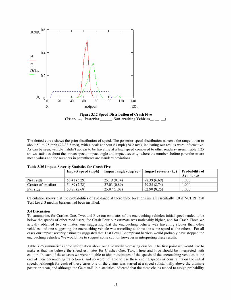
31

Figure 3.12 Speed Distribution of Crash Five

(Prior….., Posterior ______ Non-crashing Vehicles__ __ __)

The dotted curve shows the prior distribution of speed. The posterior speed distribution narrows the range down to about 50 to 75 mph (22-33.5 m/s), with a peak at about 63 mph (28.2 m/s), indicating our results were informative. As can be seen, vehicle 1 didn’t appear to be traveling at a high speed compared to other roadway users. Table 3.25 shows statistics about the impact speed, impact angle and impact severity, where the numbers before parentheses are mean values and the numbers in parentheses are standard deviations. Table 3.25 Impact Severity Statistics for Crash Five Impact speed (mph) Impact angle (degree) Impact severity (kJ) Probability of

Avoidance Near side 58.41 (3.29) 25.19 (0.74) 78.39 (6.69) 1.000 Center of median 54.89 (2.78) 27.03 (0.89) 79.25 (8.74) 1.000 Far side 50.85 (2.68) 25.87 (1.08) 62.90 (8.25) 1.000 Calculation shows that the probabilities of avoidance at these three locations are all essentially 1.0 if NCHRP 350 Test Level 3 median barriers had been installed. 3.4 Discussion To summarize, for Crashes One, Two, and Five our estimates of the encroaching vehicle's initial speed tended to be below the speeds of other road users, for Crash Four our estimate was noticeably higher, and for Crash Three we actually obtained two estimates, one suggesting that the encroaching vehicle was travelling slower than other vehicles, and one suggesting the encroaching vehicle was travelling at about the same speed as the others. For all cases our impact severity estimates suggested that Test Level 3-compliant barriers would probably have stopped the encroaching vehicles. We would like to suggest some caution however in interpreting these results. Table 3.26 summarizes some information about our five median-crossing crashes. The first point we would like to make is that we believe the speed estimates for Crashes One, Two, Three and Five should be interpreted with caution. In each of these cases we were not able to obtain estimates of the speeds of the encroaching vehicles at the end of their encroaching trajectories, and so were not able to use these ending speeds as constraints on the initial speeds. Although for each of these cases one of the chains was started at a speed substantially above the ultimate posterior mean, and although the Gelman/Rubin statistics indicated that the three chains tended to assign probability

32

to the same ranges of variables values, our experience with Crash Three, where different ranges of initial speed were found, suggests this caution. That is, it may still be possible that combinations of variable values consistent with higher speeds may have some undiscovered posterior probability, and these would be uncovered if we could place tighter bounds on the ending speeds. Our experience with Crash Four, where it was possible to constrain the ending speed, tends to confirm this. Second, looking at Table 3.15 for Crash Three, where we found evidence for two different ranges of initial speeds, we see that the impact angles still tend to be about the same despite the differences in impact speeds. This is not unexpected since the diagnostic points for this crash (and the other four) constrain the possible ranges for these angles. This suggests our impact angles estimates tend to be robust, and if these angles tend to be below the 25o value used to define Test Level 3, the encroachment would be prevented at higher impact speeds. For example, a 2000 kg vehicle striking barrier at 20o would have to be travelling at better than 70 mph in order to generate an impact severity of 128 kJ. Table 3.26 shows the rough ranges of impact angles for our five crashes. Looking these we see that that for Crashes Two, Three, and Four the impact angles tend to be below 25o, indicating that our conclusion that barriers would probably have stopped these vehicles is still likely to hold for higher speeds. For Crashes One and Five on the other hand the estimated impact angles are closer to the 25o standard, so our conclusions are less robust. Overall, Crashes Two, Three and Four would probably have been prevented by Test Level 3-compliant barriers, while for Crashes One and Five the effectiveness of barriers is uncertain. This assessment is summarized in the Barrier Prevent? column of Table 3.26. Table 3.26 Summary Information about Five Median-Crossing Crashes Crash Number

LCR Number Date/Time Highway Weather/ Road

Impact Angle (degrees)

Barrier Prevent?

Seatbelt Used?

1 97508233 06/13/1997 12:46 PM

MNTH 65 Dry 23-37 Uncertain Yes

2 99603874 08/03/1999 3:45 PM

ISTH 94 Wet 16-26 Probably Yes Yes

3 001000123 01/05/2000 4:09 PM

ISTH 35 Snow 18-22 Probably Yes Yes

4 00400239 01/05/2000 5:55 AM

USTH 61 Dry 11-12 Yes No

5 99105961 12/22/1999 12:49 PM

ISTH 90 Dry 25-28 Uncertain Yes

33

CHAPTER FOUR EXPERT ASSESSMENT OF EXTENDED SAMPLE

As indicated in Chapters One and Two, identifying causal factors for road crashes involves first determining whether or not a factor of interest was present, and second testing whether or not that factor was necessary for the occurrence of the crash. The degree of formalization used in either of these stages can vary, from the relatively informal identification of "contributing factors" on a standard accident report form to the detailed simulation and experimental testing sometimes used to determine probable causes of passenger aircraft crashes. This chapter describes a study in which teams of safety professionals reviewed a sample of fatal Minnesota crashes, using the information included in the standard accident reporting form to identify plausible causal factors and to recommend possible countermeasures. 4.1 Review of Clinical Crash Assessment Arguably the most extensive effort at identifying causes of road crashes was the Tri-Level Study, conducted between 1972 and 1977 by the Institute for Research in Public Safety at Indiana University. This study is the source of the oft-quoted statistic that driver-related factors were probable causes in about 93% of crashes; roadway and other environmental factors were probable causes in about 34% of crashes; and vehicle-related factors were causal in only about 13% of crashes. The term “Tri-Level” refers to the level of detail with which data were collected. What the researchers called Level A consisted of compiling standard police accident reports, vehicle registration and licensing data, and conducting surveys of the driving population for the study area in Monroe County, Indiana. For Level B, teams of technicians were available on-call and visited crash scenes in order to interview the involved parties, inspect the involved vehicles, and collect physical data from the crash scene. Afterwards, the teams carried out structured identifications of possible causal factors for each of their crashes. A total of 2238 crashes were investigated at Level B over the course of the study. At Level C, a subset of 420 of these crashes was independently reviewed by a multi-disciplinary of teams, which included a human factors specialist, an automotive engineer, and a crash reconstruction expert. After reviewing crashes, the multi-disciplinary team met and determined group conclusions concerning causal factors. Although the investigations carried out for Levels B and C were extensive, and often involved the use of crash reconstruction methods to determine how a crash happened, determining whether a factor was causal, i.e. if "had the factor not been present in the accident sequence, the accident would not have occurred," was based primarily on expert judgement, rather than on counterfactual simulations. The experts who carried out this work were hired staff who participated over periods of months or years. At about the same time as the Tri-Level Study, the Highway Safety Research Center at the University of North Carolina carried out a study of the relative prevalence of "unsafe driving actions" (UDA) (Lohman et al 1976). The primary data source for this study was a sample of approximately 400 computerized crash records, each of which was supplemented with the narrative provided by the investigating officer. Each sampled crash was first studied independently by each of two investigators who identified which of a pre-determined list of driving actions were possible causal factors. If the two investigators were in agreement their identifications were recorded, otherwise they attempted to reach a consensus. If consensus was

34

not reached the crash was treated as unclassifiable. Unlike the Tri-Level Study the UDA study was carried out using only the information available on a police accident report. Like the Tri-Level Study however, the experts who reviewed these reports were hired staff who participated over periods lasting several months. Finally, Vianno and Ridella (1996) investigated possible causal factors in 131 fatal crashes involving the deaths of front-seat occupants restrained by lap-shoulder belts. The data available for each of these crashes consisted of the results from technical at-scene investigations, including witness accounts, measurements, and photographs. The researchers then attempted to classify these crashes into scenarios according to what type of preventive actions might have been available to the driver of the vehicle with a fatal injury. The most frequent scenario, about 30% of the total, was called "nothing to do" since a random or negligent action on the part of another driver occurred so suddenly that no evasive action was possible. The second most frequent scenario, about 11% of the total, was called "rocket ship" and involved a single-vehicle collision by a speeding, young male driver. The study's authors did not provide an explicit description of who carried out these assessments and how long this took, but as both authors were employees of General Motors Corporation at the time the study was conducted it seems reasonable to conclude that the assessments were done by the authors as part of their regular employment. To summarize, in two of the above studies, the Tri-Level Study and that by Vianno and Ridella, the primary crash data were provided by detailed at-scene investigations and follow-ups, while for the UDA study police accident reports including the officer's narrative and scene sketch were used. In each of the three studies the opinions of professional experts were used to identify possible causal factors for the crashes, and in each the experts were paid to participate over extended periods of time. In each of these studies the "if-then" assessment as to whether or not some feature was a causal factor was generally done subjectively, without formal simulation modeling. Finally, the UDA study focused entirely on driver actions and so would not be suitable, without additional analyses, for identifying roadway-related causal factors or countermeasures. 4.2 Selection of Assessment Methodology A main constraint for the current study was that although it was possible to obtain a reasonably large (i.e. 20-25) number of safety professionals to participate as experts, these individuals would not be supported directly by the project and so their availability would be limited to one day. Given this constraint, direct application of the methods used in the above three studies was not feasible, and it was necessary to identify an alternative assessment methodology. The requirements placed on this methodology were: (1) It should be possible to use it with the information (including the narrative and diagram) on a

State of Minnesota Traffic Accident Report form. (2) It should be simple enough that a team of 3-4 people could apply it to a reasonable number

of crashes in a reasonable amount of time. The research team defined "reasonable" as 10-15 crashes in 6-8 hours.

(3) It should produce a clear identification of the sequence of causes which produced the crash, (4) It should readily lend itself to brainstorming about countermeasures.

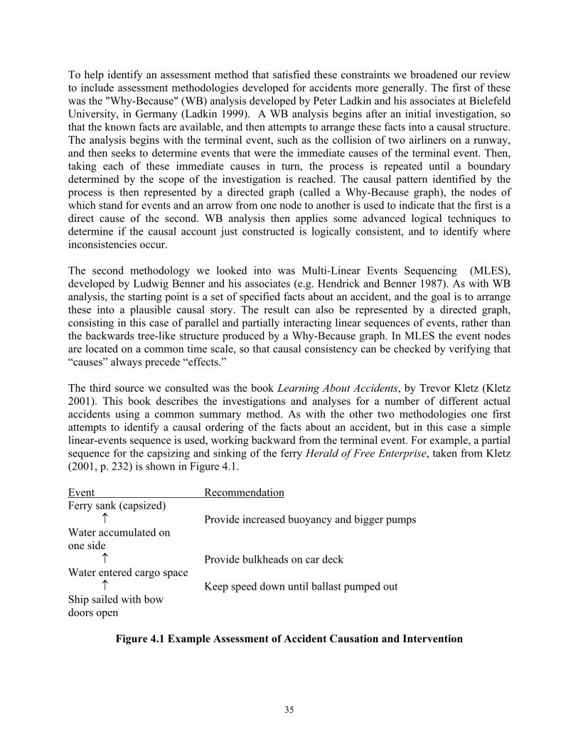
35

To help identify an assessment method that satisfied these constraints we broadened our review to include assessment methodologies developed for accidents more generally. The first of these was the "Why-Because" (WB) analysis developed by Peter Ladkin and his associates at Bielefeld University, in Germany (Ladkin 1999). A WB analysis begins after an initial investigation, so that the known facts are available, and then attempts to arrange these facts into a causal structure. The analysis begins with the terminal event, such as the collision of two airliners on a runway, and then seeks to determine events that were the immediate causes of the terminal event. Then, taking each of these immediate causes in turn, the process is repeated until a boundary determined by the scope of the investigation is reached. The causal pattern identified by the process is then represented by a directed graph (called a Why-Because graph), the nodes of which stand for events and an arrow from one node to another is used to indicate that the first is a direct cause of the second. WB analysis then applies some advanced logical techniques to determine if the causal account just constructed is logically consistent, and to identify where inconsistencies occur. The second methodology we looked into was Multi-Linear Events Sequencing (MLES), developed by Ludwig Benner and his associates (e.g. Hendrick and Benner 1987). As with WB analysis, the starting point is a set of specified facts about an accident, and the goal is to arrange these into a plausible causal story. The result can also be represented by a directed graph, consisting in this case of parallel and partially interacting linear sequences of events, rather than the backwards tree-like structure produced by a Why-Because graph. In MLES the event nodes are located on a common time scale, so that causal consistency can be checked by verifying that “causes” always precede “effects.” The third source we consulted was the book Learning About Accidents, by Trevor Kletz (Kletz 2001). This book describes the investigations and analyses for a number of different actual accidents using a common summary method. As with the other two methodologies one first attempts to identify a causal ordering of the facts about an accident, but in this case a simple linear-events sequence is used, working backward from the terminal event. For example, a partial sequence for the capsizing and sinking of the ferry Herald of Free Enterprise, taken from Kletz (2001, p. 232) is shown in Figure 4.1. Event Recommendation Ferry sank (capsized) ↑ Provide increased buoyancy and bigger pumps Water accumulated on one side ↑ Provide bulkheads on car deck Water entered cargo space ↑ Keep speed down until ballast pumped out Ship sailed with bow doors open

Figure 4.1 Example Assessment of Accident Causation and Intervention

36

The arrow connecting two events in the sequence means that there is good reason to believe that the preceding event was a causal factor for the succeeding one. For example, we would be inclined to agree that given that the ferry capsized and given that water accumulated on one side, if the water hadn't accumulated on one side the ferry wouldn't have capsized. Kletz also lists, in a parallel column, possible interventions that could have broken the causal sequence at that point. For example, given that water entered the cargo space, had bulkheads been provided on the ferry's car deck the water would not have accumulated on one side. Finally, in September 2003 the PI for this project attended the Second Workshop on the Investigation and Reporting of Incidents and Accidents, sponsored by the National Aeronautics and Space Administration and by the National Transportation Safety Board (Hayhurst and Holloway 2003). The conference featured presentations on a variety of methods which reduce some of the subjectivity inherent in accident investigation and there was a strong emphasis on automated and/or artificial intelligence-based approaches. Most of this work is at an experimental stage however, and did not (at least at that time) appear to have the flexibility and ease of use required for this project. Based on this review, it was decided that an adaptation of Kletz's method had the best chance of meeting the conditions for this project. At the June 2003 meeting of the project's Technical Advisory Panel (TAP), the method was tried out using the TAP as an expert panel, in order to get a rough idea of how easy it was to teach the method and how long an assessment might take. Based on this test, it appeared the method could be taught relatively quickly (in 1-2 hours) and that it was reasonable to expect that on average a three-person team could process a crash in about thirty minutes. In September 2004 the research team met with the project's Mn/DOT liaisons and conducted an additional test of the accident summarization procedure, which resulted in several useful ideas for streamlining and clarifying the methodology. A description of the method, with examples, was then prepared and ultimately sent to the members of the expert panel. This document, which includes instructions, a blank recording form, and examples, can be found in Appendix B of this report. 4.3 Drawing the Extended Sample and Forming the Expert Panel Having selected an assessment procedure, the next task was to select a set of crashes to be evaluated by the expert panel. To this end, during summer 2004 Mn/DOT personnel provided the research team with a spreadsheet containing crash data for all fatal crashes occurring on state highways during the years 2000-2003. Statistical summaries of the accident features were prepared by the research team and forwarded to the project's technical representatives, and it was decided that a simple random sample of the fatal accidents should capture the types of crashes of interest. Due to changes in the accident report form, it was also decided to restrict sampling to the years 2000-2002. A random number generator was then used to randomly select 100 crash numbers from the crash file, and these sampled records were written to a separate spreadsheet. This sample file was forwarded to the project's technical representatives, and in September 2004 the researchers and Mn/DOT made copies of the police reports for each sampled crash, and prepared packets for each of five expert panel teams.

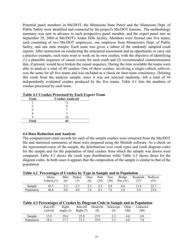
37

Potential panel members in Mn/DOT, the Minnesota State Patrol and the Minnesota Dept. of Public Safety were identified and contacted by the project's Mn/DOT liaisons. The methodology summary was sent in advance to each prospective panel member, and the expert panel met on September 29, 2004 at Mn/DOT's Arden Hills facility. Members were formed into five teams, each consisting of two Mn/DOT employees, one employee from Minnesota's Dept. of Public Safety, and one state trooper. Each team was given a subset of the randomly sampled crash reports. After instruction on conducting the structured assessment and an opportunity to carry out a practice example, each team went to work on its own crashes, with the objective of identifying (1) a plausible sequence of causal events for each crash and (2) recommended countermeasures that, if present, would have broken the causal sequence. During the time available the teams were able to analyze a total of 49 crashes. One of these crashes, involving a single-vehicle rollover, was the same for all five teams and was included as a check on inter-team consistency. Deleting this crash from the analysis sample, since it was not selected randomly, left a total of 44 independently evaluated crashes produced by the five teams. Table 4.1 lists the numbers of crashes processed by each team. Table 4.1 Crashes Processed by Each Expert Team

Team Crashes Analyzed 1 11 2 9 3 7 4 7 5 10

Total 44 4.4 Data Reduction and Analysis The computerized crash records for each of the sample crashes were extracted from the Mn/DOT file and statistical summaries of these were prepared using the Minitab software. As a check on the representativeness of the sample, the distributions over crash types and crash diagram codes for the sample and for the population of fatal crashes from which the sample was drawn were compared. Table 4.2 shows the crash type distributions while Table 4.3 shows those for the diagram codes. In both cases it appears that the composition of the sample is similar to that of the population Table 4.2 Percentages of Crashes by Type in Sample and in Population

Motor Vehicle (1)

Bike (6)

Pedest. (7)

Deer (8)

Pole (25)

Tree (30)

Bridge Pier (31)

Roadside (37)

Rollover (51)

Sample 45.5 2.3 2.3 2.3 2.3 6.8 4.6 11.4 22.7 Population 46.8 0.8 4.0 1.0 0.1 7.0 2.0 5.0 23.6

Table 4.3 Percentages of Crashes by Diagram Code in Sample and in Population

Run-Off Left (4)

Right Angle (5)

Run-off Right (7)

Head-On (8)

Sideswipe (9)

Other (90)

Unknown (98)

Sample 15.9 29.6 25.0 15.9 2.3 4.6 6.8 Population 18.6 17.7 21.2 19.0 2.3 6.0 7.0

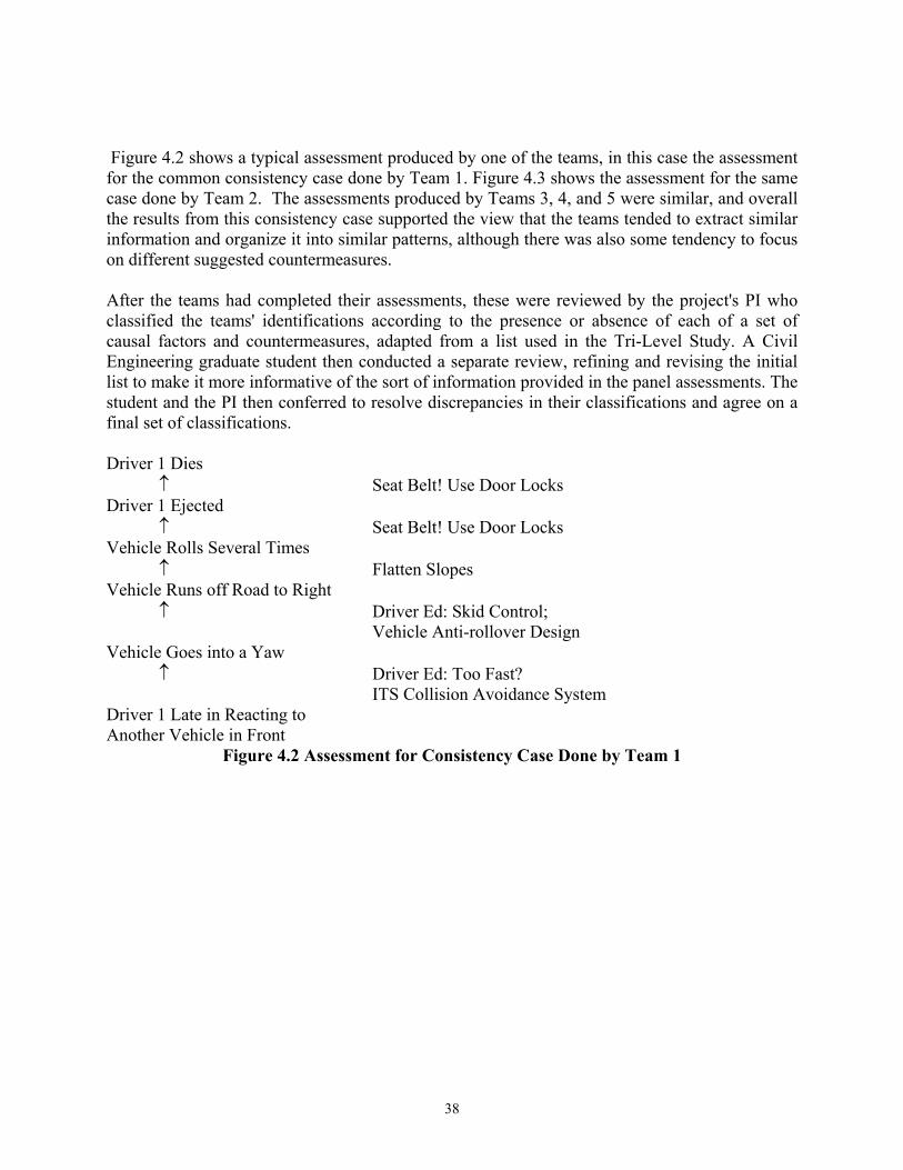
38

Figure 4.2 shows a typical assessment produced by one of the teams, in this case the assessment for the common consistency case done by Team 1. Figure 4.3 shows the assessment for the same case done by Team 2. The assessments produced by Teams 3, 4, and 5 were similar, and overall the results from this consistency case supported the view that the teams tended to extract similar information and organize it into similar patterns, although there was also some tendency to focus on different suggested countermeasures. After the teams had completed their assessments, these were reviewed by the project's PI who classified the teams' identifications according to the presence or absence of each of a set of causal factors and countermeasures, adapted from a list used in the Tri-Level Study. A Civil Engineering graduate student then conducted a separate review, refining and revising the initial list to make it more informative of the sort of information provided in the panel assessments. The student and the PI then conferred to resolve discrepancies in their classifications and agree on a final set of classifications. Driver 1 Dies ↑ Seat Belt! Use Door Locks Driver 1 Ejected ↑ Seat Belt! Use Door Locks Vehicle Rolls Several Times

↑ Flatten Slopes Vehicle Runs off Road to Right

↑ Driver Ed: Skid Control; Vehicle Anti-rollover Design

Vehicle Goes into a Yaw ↑ Driver Ed: Too Fast?

ITS Collision Avoidance System Driver 1 Late in Reacting to Another Vehicle in Front

Figure 4.2 Assessment for Consistency Case Done by Team 1

39

Driver Killed ↑ Primary Seat Belt Driver Ejected ↑ Primary Seat Belt Law-Use Seat Belt Vehicle Rolled ↑ Flatten Slope Vehicle Slid into Ditch ↑ Flatten In-slope Vehicle Left Roadway ↑ Barrier Vehicle Went out of Control ↑ Reduce Speed for Roadway Condition Vehicle Steered Right to Avoid another Vehicle ↑ Pay Attention; Reduce Speed Driver Distracted or Inattentive

Figure 4.3 Assessment for Consistency Case Done by Team 2 4.5 Results Table 4.4 lists causal factors together with the frequencies with which these were identified in the 44 sample crashes. In 18 of the 44 crashes, roughly 40% of the total, the expert panel identified misuse of seatbelts (or other restraints) as a causal factor in the fatal outcome of the crash. In 14 of the 44, roughly 32% of the total, driver inexperience was identified as a causal factor. The next most frequent causal factor was misjudging a gap, identified in 16% of the crashes, followed by older driver and alcohol involvement, each with of which appeared in about 14% of the crashes. Table 4.4 Causal Factors Identified by Panel Causal Factor Count Percent Restraint Misuse 18 40.0 Alcohol/Intoxication 6 13.6 Older Driver 6 13.6 Driver Inattention 2 4.6 Gap Misjudgement 7 15.9 Improper Maneuver 1 2.3 Improper Evasive Action 6 13.6 Dozing/Sleeping 5 11.4 Overcompensation 1 2.3 Driver Inexperience 14 31.8 Excessive Speed 5 11.4 Weather/Road Condition 4 9.1

40

Table 4.5 gives a similar tabulation of recommended countermeasures. Unlike the causal factors, which focus almost exclusively on driver actions, the recommended countermeasures show a strong emphasis on roadway-related improvements. For example, the most frequently recommended countermeasure was the provision of rumble strips, recommended for about 52% of the cases. The next most frequent, at about 34% was improvement of roadside cross-slopes, while some form of signing change was recommended in about 32% of the cases. Table 4.5 Countermeasures Identified by Panel Countermeasure Count Percent Rumble Strips 23 52.3 ITS-related 5 11.4 Speed Limit 2 4.6 Improve Clear Zone 10 22.7 Improve Control 1 2.3 Median Barrier 3 6.8 Improve Cross-Slope 15 34.1 Add Sign 14 31.8 Install Guardrail 8 18.2 Deer Fence 1 2.3 A recommended practice for identifying safety improvements (e.g. FHWA 1981) involves first identifying sites with atypically high crash experiences and then identifying the predominant types of crashes for each of these locations. For each crash type one can then use tables which list possible causes and suggested countermeasures to help design a safety intervention for a site. In order to support similar analyses for fatal rural crashes, the research team first linked the 44 crashes analyzed by the expert panel with the computerized crash records provided by Mn/DOT. This allowed us to determine whether associations existed between the information included in the standard crash record and the causal factors and countermeasures identified by the expert panel. If such associations exist then a safety analyst faced with attempting to reduce the frequency of a crash type could use these results to identify possible causal factors and countermeasures. Table 4.6 displays a cross tabulation of the code entered for crash type with the causal factors identified for the crashes. For example, looking at the second column in Table 4.6, 20 of the 44 crashes in our sample were typed as "Collision with Motor Vehicle" and of these, seven had "Restraint Misuse" identified by the panel as a causal factor, one had alcohol as a causal factor, and four had older-driver issues identified. Because more than one causal factor can be identified for a crash, the total number of causal factors identified for a type of crash does not necessarily equal the total number of crashes in that type. Looking at the last column, 10 of our sample crashes were coded as "Rollovers" and of these seven has "Restraint Misuse" identified as a causal factor and four had alcohol/intoxication identified. If there was no relationship between crash type and the identified causal factors one would expect to find similar relative frequencies of casual factors across crash types, and this is clearly not the case. For a fatal crash typed as "Collision with Motor Vehicle" the most probable causal factors appear to "Restraint Misuse,"

41

"Gap Misjudgment," and "Driver Inexperience." For a crash typed as "Rollover" the most probable causal factor is "Restraint Misuse," followed by "Alcohol/Intoxication" and "Excessive Speed." Table 4.7 shows a similar cross-tabulation of each crash's diagram code versus causal factors. Of the seven sample crashes coded as "Run-off Left," six had "Restraint Misuse" identified as a causal factor and four had "Excessive Speed" so identified. Of the seven crashes coded as "Head-on" four had "Driver Inexperience" identified as a causal factor. Table 4.6 Cross Tabulation of Panel-Identified Causal Factors with Crash Type

Motor Vehicle (1)

Bike (6)

Ped. (7)

Deer (8)

Pole (25)

Tree (30)

Bridge Pier (31)

Road- side (37)

Roll- over (51)

Total 20 1 1 1 1 3 2 5 10 Restraint Misuse 7 0 0 0 0 2 0 2 7 Alcohol/Intoxication 1 0 0 0 0 0 0 1 4 Older Driver 4 0 0 0 1 0 0 0 1 Driver Inattention 1 0 0 0 0 0 0 1 0 Gap Misjudgment 7 0 0 0 0 0 0 0 0 Improper Maneuver 0 1 0 0 0 0 0 0 0 Improper Evasive Action 5 0 0 0 0 0 0 0 1

Dozing/Sleeping 2 0 0 0 0 1 0 0 2 Overcompensation 0 0 0 0 0 0 0 0 1 Driver Inexperience 7 0 1 0 0 1 1 2 2 Excessive Speed 2 0 0 1 0 1 1 2 4 Weather/Road 3 0 0 0 0 0 0 0 1

Table 4.7 Cross-Tabulation of Panel-Identified Causal Factors with Diagram Code Run-Off

Left (4) Right

Angle (5) Run-off Right (7)

Head-On (8)

Sideswipe (9)

Other (90)

Unknown(98)

Total 7 13 11 7 1 2 3 Restraint Misuse 6 4 4 3 0 1 0 Alcohol/Intoxication 1 1 3 0 0 1 0 Older Driver 0 3 2 1 0 0 0 Driver Inattention 0 1 0 1 0 0 0 Gap Misjudgment 0 7 0 0 0 0 0 Imp. Maneuver 0 0 0 0 0 0 1 Imp. Evasive Action 1 4 0 1 0 0 0 Dozing/Sleeping 1 1 1 0 1 1 0 Overcompensation 1 0 0 0 0 0 0 Driver Inexperience 2 3 4 4 0 0 1 Excessive Speed 4 1 3 2 0 0 1 Weather/Road 1 2 0 1 0 0 0

42

Table 4.8 shows a cross-classification of crash type with recommended countermeasure. Of the 20 sample crashes involving collisions with other motor vehicles, seven had "Rumble Strips" identified as a possible countermeasure while eight had some sort of signage change identified as a possible countermeasure. Finally, Table 4.9 shows a cross-tabulation of recommended countermeasures with crash-diagram codes. Table 4.8 Cross-Tabulation of Panel-Identified Countermeasures with Crash Type Motor

Vehicle (1) Bike (6)

Ped. (7)

Deer (8)

Pole (25)

Tree (30)

Bridge Pier (31)

Roadside (37)

Rollover (51)

Total by Type 20 1 1 1 1 3 2 5 10 Rumble Strips 7 0 0 0 1 2 2 4 7 ITS-related 4 0 0 1 0 0 0 0 0 Speed Limit 2 0 0 0 0 0 0 0 0 Imp. Clear Zone 1 0 0 1 1 3 0 1 3 Improve Control 1 0 0 0 0 0 0 0 0 Median Barrier 3 0 0 0 0 0 0 0 0 Imp. Cross-slope 2 0 0 0 1 0 0 4 8 Add Sign 8 0 0 0 0 2 0 2 2 Install Guardrail 1 0 0 0 0 1 1 1 4 Deer Fence 0 0 0 1 0 0 0 0 0 Table 4.9 Cross-Tabulation of Panel-Identified Countermeasures with Diagram Code Run-Off

Left (4) Right

Angle (5) Run-off Right (7)

Head-On (8)

Sideswipe (9)

Other (90)

Unknown (98)

Total by Diagram Code 7 13 11 7 1 2 3

Rumble Strips 3 3 11 3 1 2 0 ITS-related 0 4 0 0 0 0 1 Speed Limit 0 2 0 0 0 0 0 Imp. Clear Zone 3 0 3 2 0 1 1 Improve Control 0 1 0 0 0 0 0 Median Barrier 0 1 0 2 0 0 0 Imp. Cross-slope 4 1 8 0 1 1 0 Add Sign 2 8 3 1 0 0 0 Install Guardrail 1 1 5 0 0 1 0 Deer Fence 0 0 0 0 0 0 1 4.6 Discussion In this chapter we first reviewed literature concerning the identification of causes in traffic and other accidents, and then described a study where teams of traffic safety professionals studied the crash reports from a sample of rural fatal crashes and identified plausible causal factors and possible countermeasures for each of these. These identifications were then classified by the research team and linked with the crash records for the sample cases. Summary tallies and cross-tabulations were prepared and presented in this chapter's Tables.

43

To interpret the results from the panel study one should bear in mind the processes of simplification and abstraction that occur when collecting and processing crash data. Each crash is first of all a unique event, but crashes tend to be related by similar features. The product of even the most detailed investigation and reconstruction of a crash is a simplified account of what actually occurred, and the summary provided on a standard accident report form is an even more extreme simplification. Finally, not all the information available on an accident report form is easily converted to computer codes for input into the crash database. Our panel study should be viewed then as an effort to extract additional information from accident report forms that is not normally included in the computerized crash record. Looking first at the identified causal factors, several clear results emerge from the panel's review. Failure to use seatbelts or restraints was implicated in 40% of the sample crashes, and driver inexperience was implicated in about 32%. Neither of these is the sort of feature that a state DOT has much direct control over. With regard to seatbelt use much has already been said. Current laws mandate seatbelt use and most vehicles warn the driver when his or her seatbelt is not fastened, so a driver's failure to use a seatbelt appears to be the product of some degree of deliberate choice. The options then are to either persuade the driver to make a different choice, or remove the element of choice from the situation. "Driver inexperience" is a vague term, and developing an effective intervention requires being more precise about what this means. A number of the cases where the panel identified "driver inexperience" as a causal factor involved maneuvers at high speeds, where the driver lost control, apparently after over-correcting, and then either collided with an oncoming vehicle or ran off the road and overturned. Over-correction also appeared to play significant role in the crashes studied in Chapters Two and Three, and this suggests that more consistent training in managing higher-speed maneuvers, and especially in what to do when a vehicle goes into a yaw, could eliminate some fatal crashes. We note that managing a yaw is not currently included as part of the driver's licensing road test. When we turn to tabulations of recommended countermeasures in Table 4.5, the most striking finding is that in 52% of the sample cases the panel believed that provision of rumble-strips could have been an effect countermeasure. Improving cross-slopes and/or improving clear zones were identified in 34% and 32% of the cases respectively, and in fact 22 of the 44 sample cases (50%) had at least one of these countermeasures identified. Similarly, installation of guardrail and provision of median barriers were identified in 18% and 7% of the cases respectively, and combined 10 of the 44 cases (23%) had at least one of these countermeasures identified. Overall, it is clear the panel believed that roadway-related countermeasures could help fatal crashes. Since safety analysts who want to use this information in the future will not generally be able to conduct their own panel studies, but will have access to crash records, it may be useful to be able to link the panel's findings with the crash records. This is what is provided in Tables 4.6-4.9. For example, suppose an engineer is tasked with determining countermeasures for roadway departure crashes. Looking at the last column in Table 4.8 we see that, in the panel's view, of the 10 rollover crashes seven were amenable to being prevented by rumble-strips and either were amenable to prevention by improving the roadway's cross-slope. This pattern is confirmed by the

44

first and third columns of Table 4.9. Of the eleven crashes involving run-off to the right, all were seen as amenable to prevention by rumble strips, as were three of the seven run-off-to-left crashes.

45

CHAPTER FIVE SUMMARY AND CONCLUSIONS

Chapter Two focussed primarily on fatal outcomes resulting from vehicle rollovers. In five of the ten crashes investigated there was good reason to believe that excessive speed was involved. In eight of the ten crashes the fatal victim was not properly using his/her seatbelt and in seven of these the fatal victim was ejected from the vehicle. In eight of the ten crashes the speeds and impact angles at hypothetical barrier locations were such that a barrier would probably have restrained the encroaching vehicle, while for two of these a Test Level 3-compliant barrier probably would not have been effective. Chapter Three focussed on median-crossing crashes. Unlike the crashes analyzed in Chapter Two, where existing reconstruction and estimation methods could be applied, analyzing the median-crossing crashes required, first, development of a vehicle trajectory simulation model and, second, figuring out how to embed the simulation model in a Gibbs sampling procedure. In one of the five crashes we investigated the encroaching driver was probably travelling at a high speed, but in four our speed estimates tended to be low compared to those of other, non-crashing drivers. These low speed estimates should be interpreted cautiously however since in each of these four a lack of scene information prevented reliable estimation of the vehicle speeds at the ends of their encroaching trajectories. For three of the five median-crossing crashes, Test Level 3-compliant barriers probably would have restrained the encroaching vehicles, and for two of these the effectiveness of barriers remains uncertain. In contrast to the crashes in Chapter Two, in four of the five median-crossing crashes the fatal victim was properly using a seatbelt. Finally in Chapter Four we described an expert panel review of 44 randomly selected fatal crashes. The panel identified misuse of restraints as a causal factor in about 40% of these, while driver inexperience was identified in about 32%. Provision of rumble strips was identified as a potential countermeasure in about 52% of these, while improvements to either the roadside's clear zone or its cross-slope were identified as potential countermeasures in about 50% of the crashes. Provision of either guardrail or a median barrier was identified in about 35%. The American Association of State Highway and Transportation Official’s (AASHTO) Roadside Design Guide points out that the advent of the Interstate and other limited access highways tended to reduce the relative frequency of head-on collisions in rural areas, but that collisions with man-made fixed objects became (relatively) more prominent. The widespread adoption of forgiving roadsides has in turn reduced the relative frequency of fixed-object fatalities, and now what we tend to see are fatalities due to rollovers and median crossings. Identifying countermeasures for these types of crashes is difficult because, unlike fixed object crashes, there is no specific point or object on which to focus attention. For median-crossing crashes the AASHTO Guide recommends two countermeasures, provision of wide medians, and provision of barriers. Table 5.1 shows speed limits, median widths (measured edge-line to edge-line from the scene diagrams), and estimated single-day traffic volumes for the six median-crossing crash sites, along with the three rollover crashes were the vehicle completely traversed the median.

46

Table 5.1 Speed Limits, Median Widths and Daily Traffic for Eight Crash Sites Speed Limit

(mph) Median Width (ft) Daily Traffic

Median crossing 1 55 71.4 41,500 Median crossing 2 70 60 25,700 Median crossing 3 70 46.5 19,000 Median crossing 4 50 51 53,000 Median crossing 5 70 66.5 8900 Median crossing 6 70 43 25,000 Rollover 1 70 60 42,000 Rollover 2 70 52 34,000 Rollover 3 70 62 23,000 In all cases, the medians were substantially wider than the 30-foot cutoff which the Roadside Design Guide recommends for considering a barrier, and most were wider than the 50-foot cutoff suggested in the Design Guide for "Barrier Not Normally Considered." The recommendation for a 30-foot clear zone can be found in the second edition of the AASHTO "Yellow Book," based on earlier findings that about 80% of out-of-control drivers regain control before traveling more than 30 lateral feet. For most of the cases we've investigated however, the median encroachment appeared to be triggered by loss of control following a steering over-correction, and by the time the vehicle encroached onto the median there was a substantial yaw component to the vehicle's motion. Since the drivers never regain control, their vehicles will traverse the median unless they either lack sufficient kinetic energy, they roll over, or they are stopped by an obstacle. What our five reconstructed median-crossing cases illustrate is that at typical highway speeds, and at relatively shallow encroachment angles (approximately 10-30 degrees), sufficient energy for traversal can be present. The good news however is that the impact severities generated by these crashes were often probably lower than that required by NCHRP 350's Test Level 3, so that a wide range of barrier designs could probably prevent crashes like these.

47

REFERENCES AASHTO (2002) Roadside Design Guide, Association of American State Highway and

Transportation Officials, Washington, DC. Baker, J. 1975 Traffic Crash Investigation Manual. Evanston, IL, Northwestern University

Traffic Institute. Balke, A.,& Pearl, J. 1994 Probabilistic evaluation of counterfactual queries. Proceedings of 12th

National Conference on Artificial Intelligence, Menlo Park, NJ, AAAI Press, 230-237. BMI, 2003 Improved Guidelines for Median Safety: Summary of State Tranportation Agency

Survey, Draft Report for NCHRP Project 17-14(2), National Cooperative Highway Research Program, Washington, DC.

Brach, R. and Brach, R.M. 2005 Vehicle Accident Analysis and Reconstruction Methods,

Warrendale, PA, SAE International. Cartwright, N. 2002 Causation: One word, many things, In S. Mitchell (ed.) Proceedings of the

2002 Benniel Meeging of the Philosophy of Science Association, 805-819. Cooperrider, N., Thomas, T., and Hammoud, S. 1990. Testing and anlaysis of vehicle rollover

behavior. SAE Technical Paper 900366, SAE, Inc. Warrendale, PA. Creutz, M. 1979. Confinement and the critical dimensionality of space-time. Physics Review

Letters, 43, 553-556. Davis, G. 1999 Using graphical Markov model and Gibbs sampling to reconstruct

vehicle/pedestrian accidents. Proceedings of the Conference Traffic Safety on Two Continents, Linkoping, Sweden, Swedish National Road and Transport Research Institute.

Davis, G. 2003 Bayesian reconstruction of traffic crashes. Law, Probability and Risk, in press. Davis, G., Davuluri, S., and Pei, J, 2004 A Case Control Study of Speed and Crash Risk

Technical Report 3: Speed as a Risk Factor in Run-off Road Crashes, Report to Intelligent Transportation Systems Institute, Univ. of Minnesota, Minneapolis, MN.

Devroye, L. 1986 Non-Uniform Random Variate Generation. Springer-Verlag New York Inc.

p41. Fambro, D., Koppa, R., Picha, D., & Fitzpatrick, K. 1998 Driver perception-brake response in

stopping sight distance situations. paper 981410 presented at 78th Annual Meeting of Transportation Research Board, Washington, DC.

48

FHWA 1981 Highway Safety Improvement Program, FHWA-TS-81-218, U.S. Dept. of Transportation, Washington, DC.

Fricke, L. (1990) Traffic Crash Reconstruction, Traffic Institute, Northwestern University,

Evanston IL. Geman, S. and Geman, D. (1984). Stochastic relaxation, Gibbs distributions and the Bayesian

restoration of images. Institute of Electrical and Electronics Engineers, Transactions on Pattern Analysis and Machine Intelligance, 6, 721-741.

Gilks W.R., Richardson S., and Spiegelhalter D.J. 1996 Markov Chain Monte Carlo in Practice.

London, UK, Chapman & Hall. Grenander, U. (1983). Tutorial in pattern theory. Report: Division of Applied Mathematics,

Brown University. Hayhurst, K., and Holloway, C., 2003, Proceedings of the Second Workshop on the Investigation

and Reporting of Incidents and Accidents, NASA Langley Research Center, Hampton, VA.

Hendrick, K., and Benner, L. 1987 Investigating Accidents with STEP, New York, Marcel

Dekker. Holland, P. 1986 Statistics and causal inference, Journal of American Statistical Association, 81,

945-970. Hoogstrate, A., and Spek, A. 2002 Monte Carlo simulation and inference in accident

reconstruction, Fifth International Conference on Forensic Statistics, Venice. Hume, D. 1748/1958 An Enquiry Concerning Human Understanding, LaSalle IL, Open Court. Kletz, T. 2001, Learning from Accidents, Third Ed. Gulf Professional Publishing, Oxford, UK. Ladkin, P. 1999, A Quick Introduction to Why-Because Analysis, available at

http:\\www.rvs.uni-bielefeld.de/research/WBA/. Lechner D. and Malaterre G, 1998 Emergency maneuver experimentation using a driving

simulator. SAE 910016. Limpert, R. 1989 Motor Vehicle Crash Reconstruction and Cause Analysis. 3rd ed. Charlottesville, VA, Michie Co. Lohman,. L., Leggett, E., Stewart, J., and Campbell B. 1976, Identification of Unsafe Driving

Actions and Related Countermeasures. Report DOT-HC-803-064, National Highway Traffic Safety Administration, Washington, DC.

49

Martinez, J., and Schlueter, R. A primer on the reconstruction and presentation of rollover accidents. SAE Technical paper 960647, SAE Inc., Warrendale, PA.

Mazzae, E.N., Barickman F., Baldwin, G.H.S., and Forkenbrock, G., 1999 Driver Crash

Avoidance Behavior with ABS in an Intersection Incursion Scenario on Dry Versus Wet Pavement. SAE 1999-01-1288.

Moser, A., Steffan H., Spek, A. & Makkinga W. 2003 Application of the Monte Carlo methods

for stability analysis within the accident reconstruction software PC-Crash. SAE 2003-01-0488.

Niederer, P. 1991 The accuracy and reliability of accident reconstruction. Automotive

Engineering and Litigation. vol. 4, (G. Peters and G. Peters, eds.) New York, Wiley and Sons, 257-303.

PC-CRASH Handbook, 2001 Institute of Forensic Research, Cracow, Poland. Pearl, J. 2000 Causality: Models, Reasoning, and Inference. Cambridge, UK, Cambridge

University Press. Pei, J. 2004 Bayesian Reconstruction of Median-Crossing Crashes and Causal Reasoning,

Master’s Thesis, Dept. of Civil Engineering, University of Minnesota, Minneapolis, MN. Poole, D. & Raftery, A. 2000 Inference for deterministic simulation models: The Bayesian

melding approach. Journal of American Statistical Association. 95,1244-1255. Ripley, B. D. (1979). Algorithm AS 137: simulating spatial patterns: dependent samples from a

multivariate density. Applied Statistics, 28, 109-112. Searle, J. The physics of throw distance in accident reconstruction, Accident Reconstruction:

Technology and Animation III, Warrendale, PA SAE Incorporated, 71-82. Stewart-Morris, M. 1995 Real time, accurate recall, and other myths. Forensic Crash

Investigation: Motor Vehicles. (T. Bohan & A. Damask, eds.) Charlottesville, VA, Michie Butterworth, 413-438.

Suomela, P. (1976). Unpublished Ph.D. thesis. University of Jyv≅skyl≅, Finland. Treat, J., Tumbas, N., McDonal, S., Shinar, D., Hume, R., Mayer, R., Stansifer, R., and

Castellan, N. 1977, Tri-Level Study of the Causes of Traffic Accidents, DOT-HS-805-084, National Highway Traffic Safety Administration, Washington, DC.

Viano D.C., & Parenteau C. 2003 Case Study of Vehicle Maneuvers Leading to Rollovers: Need

for a Vehicle Test Simulating Off-Road Excursions, Recovery and Handling.SAE 2003-01-0169.

50

Viano, D., and Ridella, S., 1996, Crash Caustion: A Case Study of Fatal Accident Circumstances and Configurations, SAE Technical Paper 960458, SAE Inc., Warrendale, PA.

Warner, C.Y., Smith, G.C., James, M.B., Germane, G.J. 1983 "Friction Applications in Crash

Reconstruction", SAE 830612. Wood, D. & O’Riordain, S. 1994 Monte Carlo simulation methods applied to accident

reconstruction and avoidance analysis. Crash Reconstruction: Technology and Animation IV. Warrendale, PA, SAE Inc, 129-136.

APPENDIX A

WINBUGS MODEL FOR ROLLOVER CRASH 7

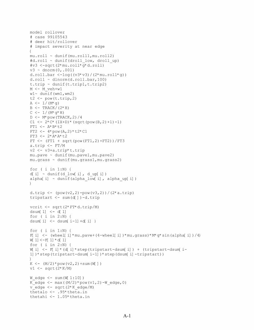
A-1

model rollover # case 99105543 # deer hit/rollover # impact severity at near edge { mu.roll ~ dunif(mu.roll1,mu.roll2) #d.roll ~ dunif(droll_low, droll_up) #v3 <-sqrt(2*mu.roll*g*d.roll) v3 ~ dnorm(0,.001) d.roll.bar <-log((v3*v3)/(2*mu.roll*g)) d.roll ~ dlnorm(d.roll.bar,100) t.trip ~ dunif(t.trip1,t.trip2) M <- M_veh+w1 w1~ dunif(wm1,wm2) t2 <- pow(t.trip,2) A <- 1/(M*g) B <- TRACK/(2*H) C <- 1/(M*g*H) D <- M*pow(TRACK,2)/4 C1 <- 2*C*(IX+D)*(sqrt(pow(B,2)+1)-1) FT1 <- A*B*t2 FT2 <- 4*pow(A,2)*t2*C1 FT3 <- 2*A*A*t2 FT <- (FT1 + sqrt(pow(FT1,2)+FT2))/FT3 a.trip <- FT/M v2 <- v3+a.trip*t.trip mu.pave ~ dunif(mu.pave1,mu.pave2) mu.grass ~ dunif(mu.grass1,mu.grass2) for ( i in 1:N) { d[i] ~ dunif(d_low[i], d_up[i]) alpha[i] ~ dunif(alpha_low[i], alpha_up[i]) } d.trip <- (pow(v2,2)-pow(v3,2))/(2*a.trip) tripstart <- sum(d[])-d.trip vcrit <- sqrt(2*FT*d.trip/M) dsum[1] <- d[1] for ( i in 2:N) { dsum[i] <- dsum[i-1]+d[i] } for ( i in 1:N) { F[i] <- (wheel[i]*mu.pave+(4-wheel[i])*mu.grass)*M*g*sin(alpha[i])/4} W[1]<-F[1]*d[1] for ( i in 2:N) { W[i] <- F[i]*(d[i]*step(tripstart-dsum[i]) + (tripstart-dsum[i-1])*step(tripstart-dsum[i-1])*step(dsum[i]-tripstart)) } K <- (M/2)*pow(v2,2)+sum(W[]) v1 <- sqrt(2*K/M) W_edge <- sum(W[1:10]) K_edge <- max((M/2)*pow(v1,2)-W_edge,0) v_edge <- sqrt(2*K_edge/M) thetalo <- .95*theta.in thetahi <- 1.05*theta.in

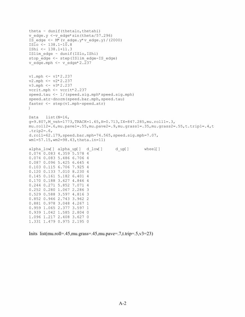
A-2

theta ~ dunif(thetalo,thetahi) v_edge.y <-v_edge*sin(theta/57.296) IS_edge <- M*(v_edge.y*v_edge.y)/(2000) ISlo <- 138.1-10.8 IShi <- 138.1+11.3 ISlim_edge ~ dunif(ISlo,IShi) stop_edge <- step(ISlim_edge-IS_edge) v_edge.mph <- v_edge*2.237 v1.mph <- v1*2.237 v2.mph <- v2*2.237 v3.mph <- v3*2.237 vcrit.mph <- vcrit*2.237 speed.tau <- 1/(speed.sig.mph*speed.sig.mph) speed.atr~dnorm(speed.bar.mph,speed.tau) faster <- step(v1.mph-speed.atr) } Data list(N=16, g=9.807,M_veh=1773,TRACK=1.65,H=0.713,IX=847.285,mu.roll1=.3, mu.roll2=.6,mu.pave1=.55,mu.pave2=.9,mu.grass1=.35,mu.grass2=.55,t.trip1=.4,t.trip2=.6, d.roll=62.179,speed.bar.mph=74.565,speed.sig.mph=7.07, wm1=57.15,wm2=98.43,theta.in=11) alpha_low[] alpha_up[] d_low[] d_up[] wheel[] 0.074 0.083 4.359 5.578 4 0.074 0.083 5.486 6.706 4 0.087 0.096 5.425 6.645 4 0.103 0.115 6.706 7.925 4 0.120 0.133 7.010 8.230 4 0.145 0.161 5.182 6.401 4 0.170 0.188 3.627 4.846 4 0.244 0.271 5.852 7.071 4 0.252 0.280 1.067 2.286 3 0.529 0.588 3.597 4.816 3 0.852 0.946 2.743 3.962 2 0.881 0.978 3.048 4.267 1 0.959 1.065 2.377 3.597 1 0.939 1.042 1.585 2.804 0 1.096 1.217 2.408 3.627 0 1.331 1.479 0.975 2.195 0 Inits list(mu.roll=.45,mu.grass=.45,mu.pave=.7,t.trip=.5,v3=23)

APPENDIX B

HANDOUT PROVIDED TO EXPERT PANEL PARTICIPANTS

B-1

B-2

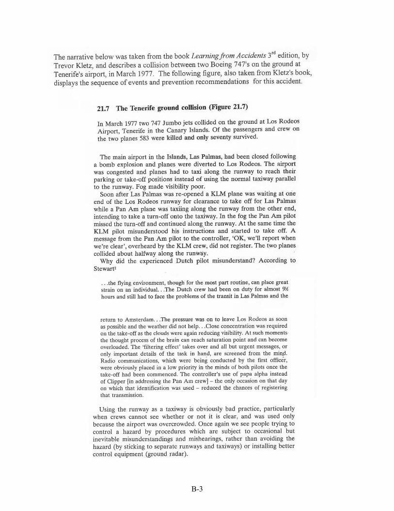
B-3

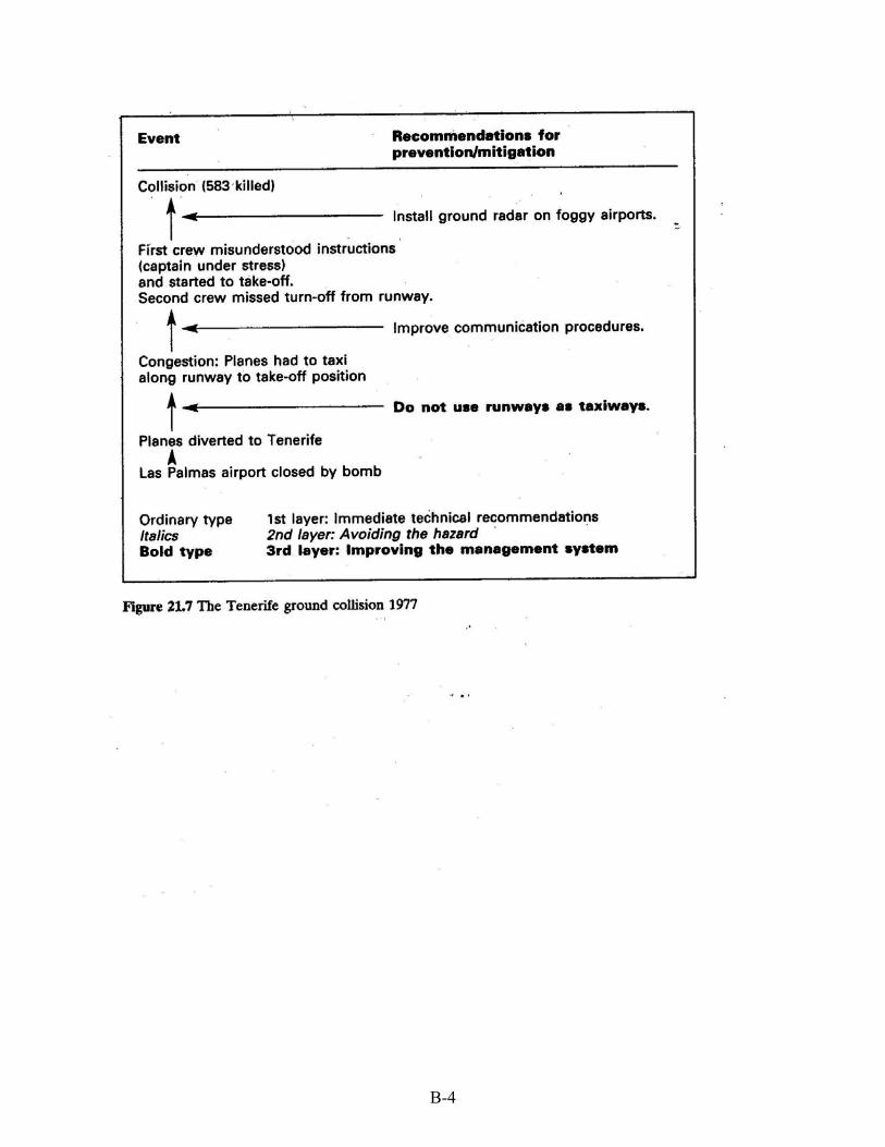
B-4

B-5

B-6

B-7