Embed Size (px)
Citation preview

Impact of Sensor Ageing on Finger-Imagebased Biometric Recognition Systems
Masterarbeit
Zur Erlangung des Diplomgrades an derNaturwissenschaftlichen Fakultät
der Paris-Lodron-Universität Salzburg
Eingereicht vonChristof [email protected]
Betreuer:Univ.-Prof. Mag. Dr. Andreas Uhl
Department of Computer SciencesUniversity of Salzburg
Jakob�Haringer�Straÿe 25020 SalzburgAUSTRIA
Salzburg, im Januar 2015


Abstract
Just like any other electronic device, image sensors show ageing e�ects over time. The most common e�ectsare hot pixels and stuck pixels which are randomly appearing, permanent defects, increasing in number overtime. These defects have the characteristics of spiky noise and degrade the image quality. The aim of thisthesis is to investigate the impact of these ageing related defects on the performance of �ngerprint, �nger-and hand vein recognition systems. For this purpose, the recognition accuracy of di�erent types of �ngerprint(minutiae-based and non-minuatie based, e.g. correlation based), �nger- and hand vein matchers (binarisationtype, keypoint based and LBP based) is evaluated in terms of the EER. As it is not possible to distinguishthe in�uence of sensor ageing related defects from other in�uences like noise, dirt, etc., the pixel defectsare simulated using images containing no or only a negligible number of pixel defects as ground-truth. Apixel model is introduced and the images are aged using an ageing simulation algorithm. The simulationparameters (defect growth rate and defect parameters) are estimated using real sensor characteristics. Thedi�erent �ngerprint, �nger vein and hand vein feature extraction and matching schemes are evaluated andcompared against each other to �nd out if they are a�ected and how they are a�ected. This should give someclues about why they are a�ected and also what can be done to make them more robust against these ageingrelated defects. According to the experimental results, there is no considerable in�uence on either of the testedschemes for a realistic number of defective pixels.
Keywords: Image sensor ageing, pixel defects, defect detection, recognition accuracy, performance evaluation,EER, �ngerprint recognition, �nger vein recognition, hand vein recognition
i

ii

Contents iii
Contents
1 Introduction . . . . . . . . . . . . . . . . . . . . . . . . . . . . . . . . . . . . . . . . . . 11.1 Image Sensor Ageing . . . . . . . . . . . . . . . . . . . . . . . . . . . . . . . . . . . . . 21.2 Existing Literature Regarding Sensor Defects . . . . . . . . . . . . . . . . . . . . . . . 21.3 In�uence on Biometric Recognition Accuracy . . . . . . . . . . . . . . . . . . . . . . . 31.4 Acronyms and Terminology . . . . . . . . . . . . . . . . . . . . . . . . . . . . . . . . . 42 Image Sensors . . . . . . . . . . . . . . . . . . . . . . . . . . . . . . . . . . . . . . . . . 92.1 Photodiodes and Photogates . . . . . . . . . . . . . . . . . . . . . . . . . . . . . . . . 92.2 CCD . . . . . . . . . . . . . . . . . . . . . . . . . . . . . . . . . . . . . . . . . . . . . . 102.3 CMOS . . . . . . . . . . . . . . . . . . . . . . . . . . . . . . . . . . . . . . . . . . . . . 102.4 Digital Cameras . . . . . . . . . . . . . . . . . . . . . . . . . . . . . . . . . . . . . . . 10
2.4.1 CFA - Colour Filter Array . . . . . . . . . . . . . . . . . . . . . . . . . . . . . . 103 Sensor Defects . . . . . . . . . . . . . . . . . . . . . . . . . . . . . . . . . . . . . . . . 133.1 Material Degradation Related Defects . . . . . . . . . . . . . . . . . . . . . . . . . . . 133.2 In-Field Defects . . . . . . . . . . . . . . . . . . . . . . . . . . . . . . . . . . . . . . . . 133.3 Mechanism Causing the Defects . . . . . . . . . . . . . . . . . . . . . . . . . . . . . . . 14
3.3.1 Spatial Distribution of Defects . . . . . . . . . . . . . . . . . . . . . . . . . . . 153.3.2 Temporal Distribution of Defects . . . . . . . . . . . . . . . . . . . . . . . . . . 15
3.4 Defect Types . . . . . . . . . . . . . . . . . . . . . . . . . . . . . . . . . . . . . . . . . 173.4.1 Pixel Defect Model (Fridrich) . . . . . . . . . . . . . . . . . . . . . . . . . . . . 173.4.2 Pixel Defect Model (Dudas and Leung) . . . . . . . . . . . . . . . . . . . . . . 203.4.3 Comparison of Defect Models . . . . . . . . . . . . . . . . . . . . . . . . . . . . 213.4.4 Stuck-High . . . . . . . . . . . . . . . . . . . . . . . . . . . . . . . . . . . . . . 213.4.5 Stuck-Low . . . . . . . . . . . . . . . . . . . . . . . . . . . . . . . . . . . . . . . 213.4.6 Stuck-Mid or Fully-Stuck . . . . . . . . . . . . . . . . . . . . . . . . . . . . . . 223.4.7 Partially-Stuck . . . . . . . . . . . . . . . . . . . . . . . . . . . . . . . . . . . . 223.4.8 Abnormal Sensitivity . . . . . . . . . . . . . . . . . . . . . . . . . . . . . . . . . 223.4.9 Hot Pixel . . . . . . . . . . . . . . . . . . . . . . . . . . . . . . . . . . . . . . . 223.4.10 Partially-Stuck Hot Pixel . . . . . . . . . . . . . . . . . . . . . . . . . . . . . . 24
3.5 Defects in Colour Images . . . . . . . . . . . . . . . . . . . . . . . . . . . . . . . . . . 243.6 Defect Identi�cation Techniques . . . . . . . . . . . . . . . . . . . . . . . . . . . . . . . 24
3.6.1 Dark Field Calibration . . . . . . . . . . . . . . . . . . . . . . . . . . . . . . . . 253.6.2 Bright Field Calibration . . . . . . . . . . . . . . . . . . . . . . . . . . . . . . . 263.6.3 Defect Identi�cation for PS and Cellphone Cameras . . . . . . . . . . . . . . . 26
3.7 Impact of Sensor Parameters on Defect Growth Rate . . . . . . . . . . . . . . . . . . . 273.7.1 Sensor Type . . . . . . . . . . . . . . . . . . . . . . . . . . . . . . . . . . . . . . 273.7.2 Sensor Area . . . . . . . . . . . . . . . . . . . . . . . . . . . . . . . . . . . . . . 273.7.3 Pixel Size . . . . . . . . . . . . . . . . . . . . . . . . . . . . . . . . . . . . . . . 283.7.4 ISO Level . . . . . . . . . . . . . . . . . . . . . . . . . . . . . . . . . . . . . . . 28
4 Defect Detection Algorithm . . . . . . . . . . . . . . . . . . . . . . . . . . . . . . . . . 314.1 Filters for Defect Identi�cation . . . . . . . . . . . . . . . . . . . . . . . . . . . . . . . 31
4.1.1 Median Filter . . . . . . . . . . . . . . . . . . . . . . . . . . . . . . . . . . . . . 314.1.2 n× n Ring Averaging Filter . . . . . . . . . . . . . . . . . . . . . . . . . . . . . 314.1.3 4NN Filter . . . . . . . . . . . . . . . . . . . . . . . . . . . . . . . . . . . . . . 324.1.4 4NN and 8NN Minimum Distance Filter . . . . . . . . . . . . . . . . . . . . . . 32
4.2 Thresholding Based Approach . . . . . . . . . . . . . . . . . . . . . . . . . . . . . . . . 324.3 Statistical Approach . . . . . . . . . . . . . . . . . . . . . . . . . . . . . . . . . . . . . 334.4 Bayesian Inference Based Approach (Dudas) . . . . . . . . . . . . . . . . . . . . . . . . 35

iv Contents
4.4.1 Image Statistics Method . . . . . . . . . . . . . . . . . . . . . . . . . . . . . . . 364.4.2 Interpolation Method . . . . . . . . . . . . . . . . . . . . . . . . . . . . . . . . 374.4.3 Extension for Hot Pixels . . . . . . . . . . . . . . . . . . . . . . . . . . . . . . . 404.4.4 Correction using Local Region Analysis . . . . . . . . . . . . . . . . . . . . . . 41
5 Ageing Simulation Algorithm . . . . . . . . . . . . . . . . . . . . . . . . . . . . . . . . 435.1 Algorithm . . . . . . . . . . . . . . . . . . . . . . . . . . . . . . . . . . . . . . . . . . . 436 Fingerprint Recognition . . . . . . . . . . . . . . . . . . . . . . . . . . . . . . . . . . . 476.1 Biometric Recognition Systems . . . . . . . . . . . . . . . . . . . . . . . . . . . . . . . 476.2 Fingerprint Recognition Systems . . . . . . . . . . . . . . . . . . . . . . . . . . . . . . 48
6.2.1 Fingerprint Sensors . . . . . . . . . . . . . . . . . . . . . . . . . . . . . . . . . . 486.2.2 Fingerprint Image Examples captured by Di�erent Sensors . . . . . . . . . . . 51
6.3 Fingerprint Anatomy . . . . . . . . . . . . . . . . . . . . . . . . . . . . . . . . . . . . . 526.4 Feature Extraction and Matching . . . . . . . . . . . . . . . . . . . . . . . . . . . . . . 53
6.4.1 Correlation Based Matcher . . . . . . . . . . . . . . . . . . . . . . . . . . . . . 536.4.2 Ridge Feature Based Matcher . . . . . . . . . . . . . . . . . . . . . . . . . . . . 546.4.3 Minutiae Based Matcher . . . . . . . . . . . . . . . . . . . . . . . . . . . . . . . 54
6.5 Factors In�uencing Recognition Accuracy . . . . . . . . . . . . . . . . . . . . . . . . . 586.5.1 Acquisition Area . . . . . . . . . . . . . . . . . . . . . . . . . . . . . . . . . . . 586.5.2 Displacement and Rotation . . . . . . . . . . . . . . . . . . . . . . . . . . . . . 586.5.3 Non-Linear Distortion . . . . . . . . . . . . . . . . . . . . . . . . . . . . . . . . 586.5.4 Pressure . . . . . . . . . . . . . . . . . . . . . . . . . . . . . . . . . . . . . . . . 586.5.5 Skin Conditions . . . . . . . . . . . . . . . . . . . . . . . . . . . . . . . . . . . . 586.5.6 Sensor Noise . . . . . . . . . . . . . . . . . . . . . . . . . . . . . . . . . . . . . 596.5.7 Fingerprint Image Enhancement . . . . . . . . . . . . . . . . . . . . . . . . . . 59
7 Finger and Hand Vein Recognition . . . . . . . . . . . . . . . . . . . . . . . . . . . . . 617.1 Finger and Hand Vein Scanners . . . . . . . . . . . . . . . . . . . . . . . . . . . . . . . 61
7.1.1 Finger Vein Scanner from Veldhuis et al. . . . . . . . . . . . . . . . . . . . . . . 617.1.2 University of Salzburg Hand Vein Scanner . . . . . . . . . . . . . . . . . . . . 63
7.2 Image Preprocessing . . . . . . . . . . . . . . . . . . . . . . . . . . . . . . . . . . . . . 637.2.1 Detecting Finger Region (LeeRegion [1]) . . . . . . . . . . . . . . . . . . . . . . 647.2.2 Finger Position Normalisation [2] . . . . . . . . . . . . . . . . . . . . . . . . . . 647.2.3 CLAHE (Contrast Limited Adaptive Histogram Equalization) . . . . . . . . . . 647.2.4 High Frequency Emphasis Filtering . . . . . . . . . . . . . . . . . . . . . . . . . 647.2.5 Circular Gabor Filter . . . . . . . . . . . . . . . . . . . . . . . . . . . . . . . . 657.2.6 Further Preprocessing . . . . . . . . . . . . . . . . . . . . . . . . . . . . . . . . 657.2.7 Best Combination . . . . . . . . . . . . . . . . . . . . . . . . . . . . . . . . . . 65
7.3 Feature Extraction and Matching Techniques . . . . . . . . . . . . . . . . . . . . . . . 667.3.1 Maximum Curvature . . . . . . . . . . . . . . . . . . . . . . . . . . . . . . . . . 667.3.2 Repeated Line Tracking . . . . . . . . . . . . . . . . . . . . . . . . . . . . . . . 687.3.3 Wide Line Detector . . . . . . . . . . . . . . . . . . . . . . . . . . . . . . . . . 697.3.4 Matching using Correlation (Miura Matcher) . . . . . . . . . . . . . . . . . . . 707.3.5 Local Binary Patterns (LBP) . . . . . . . . . . . . . . . . . . . . . . . . . . . . 707.3.6 Template Matching . . . . . . . . . . . . . . . . . . . . . . . . . . . . . . . . . . 717.3.7 SIFT / SURF . . . . . . . . . . . . . . . . . . . . . . . . . . . . . . . . . . . . . 71
8 Experimental Setup . . . . . . . . . . . . . . . . . . . . . . . . . . . . . . . . . . . . . 738.1 Fingerprint Database . . . . . . . . . . . . . . . . . . . . . . . . . . . . . . . . . . . . . 73
8.1.1 Casia 2009 and 2013 . . . . . . . . . . . . . . . . . . . . . . . . . . . . . . . . . 738.1.2 Sensor Identi�cation . . . . . . . . . . . . . . . . . . . . . . . . . . . . . . . . . 738.1.3 FVC2004 Dataset . . . . . . . . . . . . . . . . . . . . . . . . . . . . . . . . . . 75

Contents v
8.2 Finger Vein Database . . . . . . . . . . . . . . . . . . . . . . . . . . . . . . . . . . . . 768.2.1 Test Procedure . . . . . . . . . . . . . . . . . . . . . . . . . . . . . . . . . . . . 76
8.3 Hand Vein Database . . . . . . . . . . . . . . . . . . . . . . . . . . . . . . . . . . . . . 778.3.1 Test Procedure . . . . . . . . . . . . . . . . . . . . . . . . . . . . . . . . . . . . 78
8.4 Simulation Settings . . . . . . . . . . . . . . . . . . . . . . . . . . . . . . . . . . . . . . 788.4.1 Defect Growth Rate . . . . . . . . . . . . . . . . . . . . . . . . . . . . . . . . . 788.4.2 Hot and Stuck Pixel Amplitudes . . . . . . . . . . . . . . . . . . . . . . . . . . 808.4.3 Simulation Parameters . . . . . . . . . . . . . . . . . . . . . . . . . . . . . . . . 82
9 Results . . . . . . . . . . . . . . . . . . . . . . . . . . . . . . . . . . . . . . . . . . . . . 859.1 Abbreviations . . . . . . . . . . . . . . . . . . . . . . . . . . . . . . . . . . . . . . . . . 859.2 Finger Vein Results . . . . . . . . . . . . . . . . . . . . . . . . . . . . . . . . . . . . . . 86
9.2.1 Sample Aged Images and Corresponding Feature Extraction . . . . . . . . . . . 869.2.2 Simulation Results . . . . . . . . . . . . . . . . . . . . . . . . . . . . . . . . . . 869.2.3 Simulation Results with Denoising . . . . . . . . . . . . . . . . . . . . . . . . . 899.2.4 Interpretation of the Results . . . . . . . . . . . . . . . . . . . . . . . . . . . . 909.2.5 Finger Vein Conclusion . . . . . . . . . . . . . . . . . . . . . . . . . . . . . . . 92
9.3 Hand Vein Results . . . . . . . . . . . . . . . . . . . . . . . . . . . . . . . . . . . . . . 929.3.1 Sample Aged Images . . . . . . . . . . . . . . . . . . . . . . . . . . . . . . . . . 939.3.2 Simulation Results . . . . . . . . . . . . . . . . . . . . . . . . . . . . . . . . . . 939.3.3 Interpretation of the Results . . . . . . . . . . . . . . . . . . . . . . . . . . . . 959.3.4 Simulation Results with Templates Aged . . . . . . . . . . . . . . . . . . . . . . 979.3.5 Hand Vein Conclusion . . . . . . . . . . . . . . . . . . . . . . . . . . . . . . . . 100
9.4 Fingerprint Results . . . . . . . . . . . . . . . . . . . . . . . . . . . . . . . . . . . . . . 1019.4.1 Sample Aged Images and Minutiae Extraction . . . . . . . . . . . . . . . . . . 1019.4.2 Simulation Results DB1 . . . . . . . . . . . . . . . . . . . . . . . . . . . . . . . 1029.4.3 Simulation Results DB2 . . . . . . . . . . . . . . . . . . . . . . . . . . . . . . . 1059.4.4 Interpretation of the Results . . . . . . . . . . . . . . . . . . . . . . . . . . . . 1089.4.5 Simulation Results with Templates aged . . . . . . . . . . . . . . . . . . . . . . 1109.4.6 Fingerprint Conclusion . . . . . . . . . . . . . . . . . . . . . . . . . . . . . . . . 111
10 Summary . . . . . . . . . . . . . . . . . . . . . . . . . . . . . . . . . . . . . . . . . . . 115References . . . . . . . . . . . . . . . . . . . . . . . . . . . . . . . . . . . . . . . . . . . . . . 117

vi Contents

1
1 Introduction
Nowadays each one of us has to authenticate oneself for many di�erent reasons. E.g. if you want towithdraw money from the cash machine, you have to enter your personal PIN in combination withyour ID card, the same if you switch on your mobile phone. At your home computer you might alsoneed a password to log in and in other situations you authenticate via your signature. But all thesetraditional methods of authentication have some disadvantages. A signature can be forged, a PIN orpassword can be forgotten or even worse it can get disclosed and an ID card can get stolen. Thatis where biometric identi�cation systems come into place. They all use some kind of biometric trait,which is unique, stable and cannot get lost or stolen. So there is no longer the need to remembercomplex passwords or carry ID cards. Biometric systems are therefore not only more secure but alsomore convenient for the users which lead to their widespread use, especially �ngerprint recognitionsystems, because they are a mature technology and quite cheap. Usage scenarios include access controlsystems, screening at airports, �ngerprint sensor at your home door and also the �ngerprint sweep-scanners which are embedded into most modern notebook computers as an alternative to passwordlog on.
If it comes to �ngerprint recognition systems, there are many solutions available on the marketsuitable for di�erent application scenarios. These are using di�erent types of scanners, e.g. opticalscanners, silicon based ones or thermal ones from which the optical scanners are the most prominenttype. Also di�erent kinds of feature extraction and matching schemes are used, most commonlyemployed are minutiae-based ones but especially for low quality �ngerprint images non-conventionalalgorithms like correlation based ones are used.
An important factor regarding the recognition accuracy of a �ngerprint identi�cation system is thequality of the input �ngerprint image. The quality can be degraded by the skin condition itself, e.g.dryness, moisture or dirt on the �nger, by improper use, e.g. uneven pressure on the sensor or unevensweeping motion but also by sensor related issues like noise and sensor ageing related pixel defects.
Moreover there are some scenarios where a �ngerprint based recognition system cannot be used,e.g. time tracking for coal mine or construction workers as the dirt on their �ngers and the abrasion ofthe �ngers makes the use of �ngerprint scanners practically impossible. A suitable alternative couldbe an iris based system, but the more practical and cheaper solutions are �nger- and hand vein basedsystems. These systems have several advantages over �ngerprint based ones. The veins are underneaththe skin so the vein pattern is resistant against forgery as the veins are only visible in infrared light.Also liveness detection is easily possible. Moreover the vein patterns are neither sensitive to abrasionnor to �nger surface conditions. But there are also some disadvantages. First of all, so far it isnot completely clear whether vein patterns exhibit su�ciently distinctive features to reliably performbiometric identi�cations in large user groups. As the currently available data sets are limited intheir size, this issue cannot be clearly answered at present state. Another major disadvantage is thecapturing device which is, due to the required transillumination principle, rather big compared to a�ngerprint sensor. Furthermore, the vein structure is in�uenced by temperature, physical activity andcertain injuries and diseases. While the impact of these e�ects on vein recognition performance hasnot been investigated in detail so far, it is clear that suitable feature extraction methods should beindependent of the vein width to compensate for corresponding variations.
There can also be other image distortions which in�uence the image quality. One of these are pixeldefects related to ageing of the image sensor used as mentioned above. These defects are point-likeand appear as spiky shot noise in the images. After thorough search of academic sources it has beendetermined that the impact of sensor ageing related pixel defects on the performance of �ngerprintand �nger- and hand vein based recognition systems, i.e. di�erent feature extraction and matchingschemes, has not yet been studied. Therefore, this evaluation is the topic of the present thesis.

2 1 Introduction
1.1 Image Sensor Ageing
These days digital imagers are everywhere, starting from consumer cameras, mobile phone cameras,surveillance cameras. But also in biometrics digital imagers are often used to capture the biometrictrait of a subject, e.g. �ngerprints, �nger- and hand vein images, iris images and face images.
The main part of a digital imager is its image sensor, which converts the incoming light into adigital signal, i.e. the output image. Just like any electronic device, an image sensor shows ageingrelated e�ects over time. An image sensor has a much bigger area compared to other electronic partsinside a digital imager, therefore it is more sensitive to external in�uences and especially to ageingprocesses. An image sensor consists of photosensitive cells, called pixels. Image sensor ageing leads todefective pixels, the main e�ects are so called hot pixels and stuck pixels. Although the probability fora single pixel to be defective is quite low, defective pixels occur in nearly every image sensor simply dueto the high number of pixels an image sensor contains. These defective pixels are visible in the outputimage and if their number increases, the quality of the output image degrades. The e�ect is similarto spiky noise in the output image. Pixel defects are permanent, their number increases continuouslyand linearly with time and they are randomly distributed over the sensor area. A distinction is madebetween factory or fabrication time defects and in-�eld defects which are present immediately afterthe manufacturing of the image sensor or �rst appear while the sensor is in use, respectively.
These defects can be corrected by a factory calibration, at which the defective pixels are simplymasked out, i.e. their output is not used, instead their value is replaced by an interpolation ofthe neighbouring good pixels. Factory mapping is not only expensive but also infeasible in manyapplication scenarios, like embedded image sensors or extraterrestrial image sensors. Therefore, theimpact of sensor ageing should be reduced to a minimum. The industry has not paid a lot of attentionon the impact of sensor ageing related defects, because most consumer cameras are replaced after 3-4years and during this time period the number of defects is rather low, except for factory time defectsbut these are always masked out in DLSRs and most consumer cameras. But the imaging devicesused in biometrics are rarely replaced so the sensor ageing related defects may have a higher impactthere.
1.2 Existing Literature Regarding Sensor Defects
Albert Theuwissen [3, 4] analysed the source causing the in-�eld sensor defects, mainly hot spots (hotpixels). He considered terrestrial cosmic ray radiation to be the main source of the pixel defects. So hedid some experiments with sensors stored at ground level, others stored at elevated level and otherswere shipped on transatlantic �ights. It is known that the intensity of the terrestrial cosmic raysis dependent on the altitude so if his assumption is true, there should be some di�erences in defectdevelopment of the 3 groups of sensors. Indeed he found di�erences which let him conclude that theneutrons of the terrestrial cosmic rays are the main source causing pixel defects in imaging sensors.Moreover, he performed some experiments at higher temperatures (storage and annealing experiments)and showed that storing the image sensors at higher temperatures than room temperature has apositive e�ect on the development of new defects (defects with high amplitudes did not occur anymore). He also showed that it is possible to anneal some existing defects by storing the image sensorat temperatures of about 110°C for 24h. This reduces the number of hot spots independent of theiramplitudes. The details of his experiments and results are described in section 3.3.
Chapman, Dudas, Leung et al. [5, 6, 7, 8, 9, 10, 11, 12, 13, 14, 15, 16, 17] did extensive research onseveral commercial cameras, i.e. DSLR, PS (point and shoot) and mobile phone cameras. They lookedfor sensor ageing related defects trying to establish cosmic ray radiation as the main causing sourceof defects. They searched for defective pixels not only manually by doing a dark-frame calibration ona regular basis and a manual inspection afterwards but also developed an automated defect tracingalgorithm [14, 13] which is able to determine the date on which the defect �rst showed up using images

1.3 In�uence on Biometric Recognition Accuracy 3
taken by the sensor. This algorithm is explained in section 4.4. They found out that the main typeof defects are hot pixels. Indeed they never found a true stuck pixel. Using the data collected duringthe measurements they did an analysis on the spatial and temporal distribution of the defects [16]. Itbecame apparent that the defects are distributed uniformly over the sensor area and the size of thefault in the silicon lattice which causes the pixel to be defective is much smaller than the size of a singlepixel (less than 2.3% of its size [13]), which indicates some type of constant stress, which the sensoris exposed to, rather than material degradation as defect source, else there would be defect clusters.It also turned out that the number of defects is increasing linearly with time (i.e. the defect rate isconstant over time, implying a Poisson process) which also indicates some kind of causal mechanismlike radiation as defect source rather than a single traumatic event or material degradation relateddefects, else the increase would be sudden or exponential, respectively. Thus they concluded thatcosmic ray radiation might be the main source causing image sensor defects. In addition they alsoevaluated the in�uence of sensor parameters like sensor area, sensor type (CCD or CMOS), pixel sizeand ISO setting on the defect growth rate and found out that the growth rate scales linearly, whichis another evidence for some kind of radiation as the source causing the defects. They also found outthat reducing the pixel size has a great impact on the defect growth rate (smaller pixels lead to moredefects) and that CCD sensors are more sensitive to the defect source than CMOS/APS ones, i.e.they develop more defects. Furthermore the ISO level has a big in�uence on the number of defects asthe ISO setting is nothing else than a numerical gain factor, which also ampli�es the defective pixelparameters, thus they become more visible at higher ISO levels and some of them might even be onlydetectable at a higher ISO setting. They were �nally able to derive an empirical formula which is apower law relationship between the defect growth rate and the sensor characteristics. The details aredescribed in section 3.7.
Jessica Fridrich [18] investigated imperfections of image sensors and how they can be used as aunique sensor �ngerprint. Among these imperfections are manufacturing time defects, defects causedby physical processes inside the camera and also defects caused by environmental factors. She focusedon the photo-response non-uniformity (PRNU) and the dark current. The PRNU is essentially a noisepattern caused by imperfections of the di�erent pixels due to the manufacturing process (physicaldimensions, quantum e�ciency and homogeneity of the silicon may vary), which is overlaid on theimage. Even if there is no exposure, a pixel may contain some free electrons causing a current �owdue to thermal e�ects, commonly denoted as dark current. This dark current increases with risingtemperature and higher exposure times. Therefore, the e�ect on the output image is dependent onthe temperature, the exposure time but also the ISO setting. If the dark current of a pixel is veryhigh, the pixel is called a hot pixel. If the pixel has a high additional o�set, which is illuminationindependent, it is called stuck pixel. She proposed a pixel output model, which is described in section3.4.1 and according to this model she derived the defect matrices based on multiple images taken withthe same sensor using the maximum likelihood method. This is done by computing the noise residualusing a custom-designed wavelet and a 3x3 median �lter. She also found out that pixel defects occurrandomly in time and space and are independent from each other. New defects appear with a constantrate, i.e. it is a Poisson process and once a defect occurs it is permanent. This is again an evidenceof cosmic rays as the source causing defects.
1.3 In�uence on Biometric Recognition Accuracy
Up until today, it is not clear if and how these sensor ageing e�ects in�uence the recognition accuracyof di�erent biometric systems. To be able to quantify the impact on the recognition accuracy, atleast two identical samples, captured at di�erent points in time, of the same person showing noother ageing related e�ects than sensor ageing, would be needed. Unfortunately it is impossible toachieve identical conditions for both captures, as there are other in�uences, e.g. misalignment, human

4 1 Introduction
ageing and environmental conditions which make the separation of the sensor ageing related impactimpossible. So it is not possible to capture real test data to evaluate the impact of sensor ageing.
This thesis proposes a method to evaluate the impact of sensor ageing on the recognition accuracyof �nger image based biometric recognition systems, i.e. �ngerprint, �nger vein and hand vein basedsystems. To overcome the problem of other in�uences than sensor ageing related defects in the testdata, an algorithm, which is able to simulate sensor ageing e�ects within images, is used to generatesimulatively aged �ngerprint, �nger vein or hand vein images, respectively. Thus a common imagedata base can be used as a starting point for the experiments. As �ground-truth� the baseline matchingperformance, i.e. recognition accuracy, of the di�erent matchers for this data base is determined �rst.This data base is then �aged� using the algorithm and the di�erent matching schemes are evaluatedusing the aged versions of the images to measure the impact of sensor ageing on the biometric system'srecognition accuracy. The parameters for the simulation (defect growth rate, types and intensities ofthe defects) are estimated using an empirical formula based on the biometric sensor's technical data.Then the results of the di�erent matchers can be evaluated and the impact of the sensor ageing relateddefects can be quanti�ed, compared against each other and also the di�erences can be investigated.
So at �rst, it reveals whether a single matcher is in�uenced by the ageing related defects or not,i.e. is the matching performance decreasing or is the matcher robust against it and the performancedoes not change at all. Through comparing to the results of the other matchers also the relationof these results can be evaluated to determine if all matchers are equally in�uenced or if there aresome that are more robust against it than others. By doing a ranking of the matcher performancesalso the question of whether this ranking is in�uenced can be decided, i.e. is the best matcher stillthe best one under the in�uence of pixel defects or does the ranking change at some point? Thisleads to another important question, do all the matchers react in the same way to the defectivepixels or are there any irregularities? So the main goal of this thesis is to investigate the in�uence ofsensor ageing related pixel defects in �ngerprint, �nger- and hand vein images on the performance ofdi�erent feature extraction and matching schemes. For �ngerprint images 2 minutiae-based matchers,one correlation-based matcher and one ridge feature-based matcher have been evaluated. For �nger-and hand vein images 5 binarisation-type approaches (trying to extract the vein pattern, creatinga binary vein image and comparing the binary images then) and a keypoint-based approach (SIFTbased) have been investigated.
The rest of this thesis is structured as follows: Section 2 describes the principle of an image sensorand also the two main sensor types, CCD and APS. Section 3 investigates the cause of sensor defects,describes the di�erent defect types and gives two di�erent pixel models describing these defects. Insection 4 a defect detection algorithm, which is able to identify defects in conventional images (nodark-�eld or bright-�eld calibration images) is presented. Section 5 describes the simulation algorithmwhich is used to generate aged images by using given defect parameters. In section 6 the di�erent�ngerprint recognition methods are outlined. Section 7 describes the di�erent feature extractionand matching methods used for �nger- and hand vein recognition. Section 8 gives an overview ofthe experimental setup and the image databases. In section 9 the results of the di�erent ageingexperiments are presented and interpreted. Section 10 �nally summarizes the �ndings of this thesisand gives an outlook on future work.
Below you will �nd an explanation of several terms and acronyms appearing in this thesis.
1.4 Acronyms and Terminology
APS Active Pixel Sensor, is one of the two major types of image sensors used in digital cameras andalso biometric sensors.
CCD Charge-Coupled Device, is the second type of image sensor commonly used.

1.4 Acronyms and Terminology 5
CMOS Complimentary Metal Oxide Semiconductor, is a technology for constructing integrated elec-tronic circuits. It is also an abbreviation for the APS sensor which is sometimes called CMOS sensor.
DSLR Digital Single Lens Re�ex camera, a digital camera combining the principle of a single-lensre�ex camera with a digital image sensor.
ISO Level The ISO level or ISO setting originates from analogue photography and describes thesensitivity of a photographic �lm to the incoming light depending on the characteristics of the �lm.The ISO level of a digital image sensor is adjusted by setting the signal gain of the sensor. A higherISO level means that the sensor is more sensitive to incoming light, i.e. images get brighter at thesame exposure time. But with an higher ISO level also the noise level is increased.
MP Megapixel, a million pixels. Used to indicate the total number of pixels of an image but alsofor the maximum possible resolution of an image sensor.
PS Point-and-Shoot camera, the most common type of digital camera used in consumer area. It isdesigned for simple and easy to use operation. Due to its simple design compared to DSLR camerasthese cameras are also cheaper than DSLRs.
Fingerprint, Finger- and Hand-Vein Images Digital images captured by a biometric sensor, i.e. a�ngerprint scanner for �ngerprint images, a �nger vein scanner for �nger vein images and a handvein scanner for hand vein images, respectively. As the impact of sensor ageing related pixel defectsshould be investigated, only optical scanners are considered in this thesis, because the sensor ageinge�ects as described in section 3 are only applicable for optical image sensors. Fingerprint sensors aredescribed in section 6.2.1. Finger- and hand vein scanners use an optical transillumination principlewith which the �nger or hand, respectively is screened using near-infrared light to render the veinsvisible. These scanners are explained in section 7.1. During the experiments regarding �ngerprintmatchers, the sample images from the Fingerprint Veri�cation Contest 2004 (FVC2004, please referto section 8.1.3 for details) were used. The experiments on �nger vein recognition were conductedon images of the University of Twente Finger Vascular Pattern Database (UTFVP, details in section8.2). For the evaluation of hand vein recognition performance a data set captured at the Universityof Salzburg (see section 8.3) was utilized.
Recognition Performance The di�erent matchers were evaluated using the sample data mentionedbefore. The recognition performance was quanti�ed in terms of the matching performance. Therefore,the procedure of the FVC2004 was adopted, which is described in section 8. In order to be ableto compute the matching performance, the matching results or matching scores, respectively, wereanalysed and the following numbers were calculated:
• False Match Rate (FMR)
• False Non Match Rate (FNMR)
• Equal Error Rate (EER)
Biometric Identi�cation A biometric identi�cation system tries to determine the identity of a sub-ject. It is given a speci�c kind of biometric trait, e.g. a �ngerprint, and compares this with all thesamples previously enrolled and stored in the data base. It returns the best match including thematching score and should also return the likelihood that the found match is correct, depending on

6 1 Introduction
the impostor matching scores and the sole genuine one. Such a system performs an 1 to n match, i.e.it matches the given input to all other samples stored in the data base.
Biometric Veri�cation Contrasting to identi�cation systems, a veri�cation system is not only givena biometric trait but also information about the claimed identity. It thus only has to compare thetrait with the one stored in the data base under the same ID. If the matching score is above a presetthreshold, the system con�rms the claimed identity, otherwise not. The �rst one is called a match,the second case is called non-match. A veri�cation system performs an 1 to 1 match, i.e. it matchesthe given input only to the sample stored in the database with the given ID, at least in theory.
Matching Score A biometric recognition system compares two samples of the same biometric trait,e.g. it gets two �ngerprint images as input and the output of the system is a matching score. Thisscore indicates either the similarity or the di�erence between the two inputs. Depending on this scorethe result of an identi�cation or a veri�cation process, respectively is determined. Using a threshold tand comparing the matching score s to this threshold, the output can either be a match (s ≥ t) or anon-match (s < t, vice versa if the score value indicates di�erence instead of similarity). Usually thematching scores are normalised to be in a range of [0, 1].
Genuine Score A genuine score is a resulting matching score of a comparison in which the giveninput corresponds to the sample stored in the data base with the same identity as the claimed inputone.
Impostor Score An impostor score is a resulting matching score of a comparison in which the giveninput does not correspond to the sample stored in the data base with claimed input identity.
False Match Rate (FMR) A false match occurs when two samples taken from a di�erent subjectare incorrectly classi�ed as originating from the same subject, e.g. two �ngerprints from di�erentpersons or �ngers are declared to be from the same �nger. Given a whole data set, the false matchrate denotes the number of false matches divided by the total number of performed matches.
False Non Match Rate (FNMR) A false non match occurs when two samples are classi�ed to befrom two di�erent subjects but actually they belong to the same subject, e.g. two �ngerprints takenfrom the same �nger are declared to be from di�erent �ngers. The false non match rate denotes thenumber of false non matches divided by the total number of performed matches for a given data set.
Equal Error Rate (EER) By adjusting the threshold within a set of matching scores, the matchingscores will either lead to a match or a non-match, both the FMR and FNMR change. The EERis the point where the FMR and FNMR have the same value. It is a performance indicator for abiometric recognition system. A low EER corresponds to low FMR and FNMR values and thus to ahigh recognition accuracy.
Simulation of Sensor Ageing During this work only the in�uence of sensor ageing related pixeldefects and no other external in�uences should be evaluated. Real �ngerprint �nger vein or hand veinimages will always contain other distortions due to �nger surface conditions, dirt on the sensor area,subject ageing, etc. Thus, in order to be able to exclude these external in�uences the sensor ageinge�ects are simulated, i.e. the pixel defects are generated arti�cially and overlaid onto the images usingthe algorithm described in section 5. Therefore, the images of the sample data sets mentioned abovewere used as a basis, i.e. as unaged images and the algorithm was applied to generate several data

1.4 Acronyms and Terminology 7
sets with di�erently aged versions of the images, which were then used to determine the matchingperformance.
Test-Run A test-run describes a run of all the matches necessary for determining the EER (genuineand impostor matches) according to the test protocol adopted from the FVC2004 for a single matcherand a single aged data set. For the �ngerprint data this results in a total of 7750 matches performed.For the �nger vein data 12740 matches and for the hand vein data set 5250 ones are performed.Afterwards, the resulting EER based on the match scores is calculated which is the result of thetest-run.

8 1 Introduction

9
2 Image Sensors
For an accurate analysis of the impact of sensor defects, at �rst some of the fundamental principlesof solid-state image sensors should be explained. This section gives a short overview of the basicworking principle of an image sensor from light detection to digital cameras. In short an image sensorconsists of an array of photosensitive cells, called pixels, and converts the incoming light �rst into aproportional voltage or current which is then converted into a digital value using an analog to digitalconverter. Although the rest of the imager system is digital, the sensor is an analog device. In anideal image sensor every pixel would be rectangular and have a uni�ed photo-response, which meanseach pixel produces the same output at the same level of incoming light. But in reality there aresome pixels that are more sensitive compared to others due to imperfections in the manufacturingprocess, these are called manufacturing time defects. Moreover there are also other e�ects, like thetemperature dependent dark current which a�ect the pixels' output. Even worse some of the pixelsmay change their photo-response characteristics over time, which are typically called in-�eld defects.This e�ect is commonly called sensor ageing.
Today there are two main types of image sensors, CCD and CMOS which are di�erent in the wayhow they convert the photons from the incoming light into electrical signals. Each of these two hasits advantages but also disadvantages which are described below.
2.1 Photodiodes and Photogates
The light detection mechanism is shared by both CCD and CMOS sensors. At the very low level thephotoelectric e�ect is the basis of light detection. If the energy of a photon from the incoming lightis large enough, its energy is absorbed by the semiconductor material, which leads to the elevation ofan electron into the conduction band, generating a free carrier. On its own this is not su�cient toconvert the incoming light into an electric current as the free carriers recombine after a short time.
The freed electrons have to be captured in an electric �eld such as it is used in a photodiode.A photodiode is a semiconductor device, much like a regular semiconductor diode, containing a p-njunction, which converts the incident light into an electric current. By applying a positive voltage it isoperated in the so called photo-conductive mode, generating a depletion layer, which also reduces theresponse time. The voltage is then removed and light which reaches through to the depletion regiongenerates free electron-hole pairs in it. Due to the built-in electric �eld these pairs are separatedand the holes and electrons are pushed to the opposite ends of the photodiode which induces anelectric current. As this current is very small, this process lasts only for a short time, which is calledthe integration time. During this time the charge is collected inside the photodiode, which is thenread, followed by a reset phase at which the positive voltage is applied again. Ideally the generatedphotocurrent should be dependent on the incident illumination only, but even in an ideal photodiodethere is a so called dark current. The dark current is a thermally generated leakage current due to theapplied reverse bias voltage, which is dependent on the temperature and the junction width, leadingto a discharge even in complete darkness. Due to impurities occurring during the production process,causing defects in the silicon lattice, this thermally generated current is not uniform and may begenerated more rapidly.
A photogate is used to convert light into an electric current and is a metal oxide semiconductorcapacitor. Its operation is similar to a photodiode, only the construction is di�erent. It consists of ap-substrate, an oxide layer and a gate electrode above this layer. Again to create a depletion regionunderneath the gate, a positive voltage is applied to the electrode. Inside this region the photonscontained in the incident light create the free electron-hole pairs during the integration time and thecurrent is read out at the end of the integration time.
10 2 Image Sensors
2.2 CCD
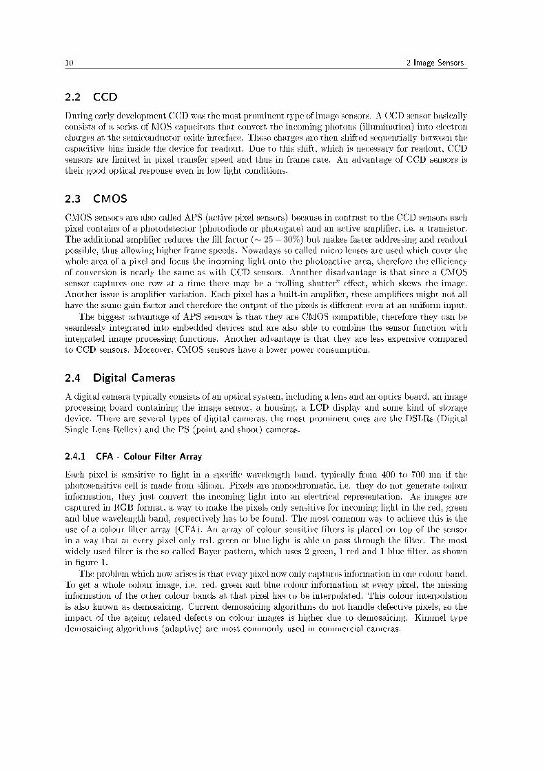
During early development CCD was the most prominent type of image sensors. A CCD sensor basicallyconsists of a series of MOS capacitors that convert the incoming photons (illumination) into electroncharges at the semiconductor-oxide interface. These charges are then shifted sequentially between thecapacitive bins inside the device for readout. Due to this shift, which is necessary for readout, CCDsensors are limited in pixel transfer speed and thus in frame rate. An advantage of CCD sensors istheir good optical response even in low light conditions.
2.3 CMOS
CMOS sensors are also called APS (active pixel sensors) because in contrast to the CCD sensors eachpixel contains of a photodetector (photodiode or photogate) and an active ampli�er, i.e. a transistor.The additional ampli�er reduces the �ll factor (∼ 25− 30%) but makes faster addressing and readoutpossible, thus allowing higher frame speeds. Nowadays so called micro lenses are used which cover thewhole area of a pixel and focus the incoming light onto the photoactive area, therefore the e�ciencyof conversion is nearly the same as with CCD sensors. Another disadvantage is that since a CMOSsensor captures one row at a time there may be a �rolling shutter� e�ect, which skews the image.Another issue is ampli�er variation. Each pixel has a built-in ampli�er, these ampli�ers might not allhave the same gain factor and therefore the output of the pixels is di�erent even at an uniform input.
The biggest advantage of APS sensors is that they are CMOS compatible, therefore they can beseamlessly integrated into embedded devices and are also able to combine the sensor function withintegrated image processing functions. Another advantage is that they are less expensive comparedto CCD sensors. Moreover, CMOS sensors have a lower power consumption.
2.4 Digital Cameras
A digital camera typically consists of an optical system, including a lens and an optics board, an imageprocessing board containing the image sensor, a housing, a LCD display and some kind of storagedevice. There are several types of digital cameras, the most prominent ones are the DSLRs (DigitalSingle Lens Re�ex) and the PS (point and shoot) cameras.
2.4.1 CFA - Colour Filter Array
Each pixel is sensitive to light in a speci�c wavelength band, typically from 400 to 700 nm if thephotosensitive cell is made from silicon. Pixels are monochromatic, i.e. they do not generate colourinformation, they just convert the incoming light into an electrical representation. As images arecaptured in RGB format, a way to make the pixels only sensitive for incoming light in the red, greenand blue wavelength band, respectively has to be found. The most common way to achieve this is theuse of a colour �lter array (CFA). An array of colour sensitive �lters is placed on top of the sensorin a way that at every pixel only red, green or blue light is able to pass through the �lter. The mostwidely used �lter is the so called Bayer pattern, which uses 2 green, 1 red and 1 blue �lter, as shownin �gure 1.
The problem which now arises is that every pixel now only captures information in one colour band.To get a whole colour image, i.e. red, green and blue colour information at every pixel, the missinginformation of the other colour bands at that pixel has to be interpolated. This colour interpolationis also known as demosaicing. Current demosaicing algorithms do not handle defective pixels, so theimpact of the ageing related defects on colour images is higher due to demosaicing. Kimmel typedemosaicing algorithms (adaptive) are most commonly used in commercial cameras.

2.4 Digital Cameras 11
Fig. 1: Bayer CFA pattern [14]
Another problem with the colour �lter array is the reduction of the overall sensitivity of the sensor.As with each �lter only one colour band is allowed to pass through and reach the sensor surface, theremaining components of the incoming illumination are lost. Only 50% of the green and 25% of theblue and red intensity is retained.

12 2 Image Sensors

13
3 Sensor Defects
Digital image sensors enjoy a widespread use today and become more and more popular. Startingfrom consumer cameras to mobile phones, cars and also other consumer electronic devices such asnotebook computers, TV sets, etc. Like every creature also electronic components age over time.Unlike other electronic components, image sensors show ageing related defects soon after fabrication.Sensor defects occur in the form of defective pixels, which show a di�erent characteristic than atmanufacturing time. Some are completely insensitive to incoming light, others add an o�set andare more sensitive to illumination than the other pixels. The accumulation of these defective pixelsdegrades the quality of the output image but fortunately they do not prevent the sensor from stillproviding useful output data. The main source causing these defective pixels is radiation. Unlike otherdevices, at which radiation causes mainly transient soft errors, i.e. errors that recover after a sensorreset or a certain amount of time, these image sensor ageing related pixel defects are permanent, i.e.they do not heal over time, their characteristics do not change and their number increases continuouslywith time.
In this chapter the di�erent types of pixel defects are explained and a pixel model to describe thedefective pixels is presented. The spatial and temporal distribution of the defects is studied, whichgives some hints indicating the source causing the defects. The e�ect of colour demosaicing on singlepixel faults is analysed, followed by an overview of di�erent defect identi�cation techniques. Finallythe impact of sensor parameters on the defect growth rate is investigated.
3.1 Material Degradation Related Defects
Defects related to material degradation are mainly caused by to limitations and impurities during themanufacturing process of the sensor. These defects make the sensor more vulnerable and lead to earlymaterial breakdown. There can be minor faults like errors in the output image but also severe faultslike a complete failure of the sensor.
Manufacture time defects are those which occur before the image sensor leaves the factory. Suchdefects exist but as the manufacturer does a so called factory calibration, i.e. generating a defect mapand using this map to mask out the defective pixels during the colour interpolation (demosaicing)step and additionally by performing a dark frame subtraction after each image capture, these defectsare not noticeable.
Defects related to material degradation that occur in-�eld are e.g. gate oxide thinning, hot carriersand electromigration. These defects are localized in a small area and will usually result in a cluster ofspatially close defects which all develop at around the same time. The number of material degradationrelated defects rises exponentially with time and as it is shown in section 3.3.1 and 3.3.2 that bothconditions do not apply for typical in-�eld pixel defects, material degradation cannot be the mainsource causing in-�eld defects. Therefore these defects are not explained in more detail here.
3.2 In-Field Defects
In contrast to manufacture time defects, in-�eld defects develop while the sensor is in use. But theynot only develop while it is in use, also while it is stored. The most prominent types of in-�elddefects are single pixel failures like hot or stuck pixels. The impact of these defects could be overcomeby performing a factory calibration. This is not only expensive but also infeasible for imagers inembedded devices and in remote sensing applications. Some researchers [13] found exclusively hotpixels and no other types of defects, which indicates that the source causing hot pixel defects doesnot lead to other defect types like stuck and abnormal sensitivity defects. Details of the defect typesare described below.

14 3 Sensor Defects
There are other types of in-�eld defects related to electrical stress, e.g. �uctuations in the supplyvoltage and also electrostatic discharge, which are not discussed here.
3.3 Mechanism Causing the Defects
According to the literature, the main mechanism causing sensor defects is cosmic ray radiation.
Albert Theuwissen [3, 4] studied the in�uence of terrestrial cosmic rays on the number and para-meters of newly generated pixel defects in image sensors. Terrestrial cosmic rays are the result of highenergy particles originating from space (primary cosmic rays) which hit the atmosphere and producesecondary particles (secondary cosmic rays). He showed that the main mechanism causing the defectsare neutrons, which are part of the terrestrial cosmic rays, that lead to displacement damage in thesilicon bulk. The energy and density of cosmic rays is dependent on the altitude, the latitude as wellas on the earth's magnetic �eld. During an air plane �ight, the density of neutrons in the cosmicray total �ux is about 100-300 times higher compared to ground level. To show that the terrestrialcosmic rays are the cause of the sensor defects, he evaluated several image sensors which were storedon-the-shelf, others were kept running and others were shipped around the world in air planes. Asthe radiation due to cosmic rays is higher during transatlantic �ights, sensors shipped by air planeshould show a higher defect rate. He indeed showed that there is an increase in the hot spot density ofthe shipped sensors compared to the stored ones (about 100 times higher which is in correlation withthe increase in neutron density). Moreover he discovered that the probability to develop hot pixelswith high amplitudes is relatively higher for sensors after the �ights. He also stored some sensors atelevated altitudes and discovered what was expected, an increase in the number of hot spots comparedto the sensors stored at sea level. In addition he stored some sensors underground, which should leadto an improvement, i.e. a lower number of hot spots, but the results of his experiment did not con�rmthis, which indicates that cosmic rays are not the only source generating new pixel defects. Leunget al. [13, 14] also noticed a similar increase in defect growth rate or defect count, respectively, aftertransatlantic �ights present at their tested cameras.
Another mechanism causing sensor defects might be the increase of the dark current level overtime. If the dark current increases, also the amplitudes of the hot pixels increase and therefore theybecome more visible.
Albert Theuwissen [3] concluded from his experiments that hot pixels with high amplitudes aremainly created due to the damage in the bulk of the silicon substrate caused by terrestrial cosmicrays. A high-energy neutron of the cosmic rays may hit a silicon atom right in its centre, which leadsto a displacement of this atom from its rigid crystal structure, creating an interstitial and a vacancy,which are unstable. They migrate to energetically favourable positions in the lattice and may becometrapped near impurity atoms due to the stress imposed on the lattice by the impurities and remainin a stable position there, creating a hot spot [4]. Hot pixels with lower amplitudes are most likelycaused due to damage created at the Si-SiO2 interface, which results in an overall increase of the darkcurrent. He also showed that the creation of new hot pixels is independent of technology, architecture,sensor type and vendor, but the amplitude of the hot pixels can depend on the sensor parameters.
In the second part of his experiments [4] he showed that also the storage temperature has anin�uence on the generation of new pixel defects. According to his results storing an image sensor athigher temperatures than room temperature results in an overall improvement, i.e. a reduction ofthe number of hot pixels with a high amplitude and reduces the generation of defects considerably.At 180° C hot pixels with a high amplitude no longer show up but the number of hot pixels with asmall amplitude increases. The best storage temperature for image sensors is between 60° C and 110°C. He concludes that there has to be an instant annealing e�ect of hot pixels generated by cosmicrays but on the other hand another mechanism causing the generation of new hot pixels at highertemperatures.

3.3 Mechanism Causing the Defects 15
In addition he performed annealing experiments with sensors usually stored at room temperatureand found out that annealing at 100° C for 24 h seems to be very e�cient in reducing the numberof hotspots. This statement is true for hot spots of all amplitudes [4]. Therefore an anneal of 24h at relatively low temperatures can be a good alternative to the storage at elevated temperatures.The overall e�ect seems to be the same. After 24h at 110° C most of the hot spots are annealed[4]. So this means that the hot pixels are not completely permanent as they can be annealed athigher temperatures. This and the in�uence of higher temperatures can by explained by the fact thatthe mobility of the vacancies and interstitial silicon atoms increases with increasing temperature, sothe chance that a vacancy and interstitial recombine becomes higher. Moreover, the energy of thevacancies becomes larger so that a vacancy is instantly released from the trap again.
3.3.1 Spatial Distribution of Defects
The spatial distribution of the defects across the sensor area follows a normal random distribution(also true among di�erent ISO levels) which means that the defect source is neither related to themanufacturing process, e.g. the design of the pixels, nor to material degradation. Material degradationwould lead to defect clusters as described above.
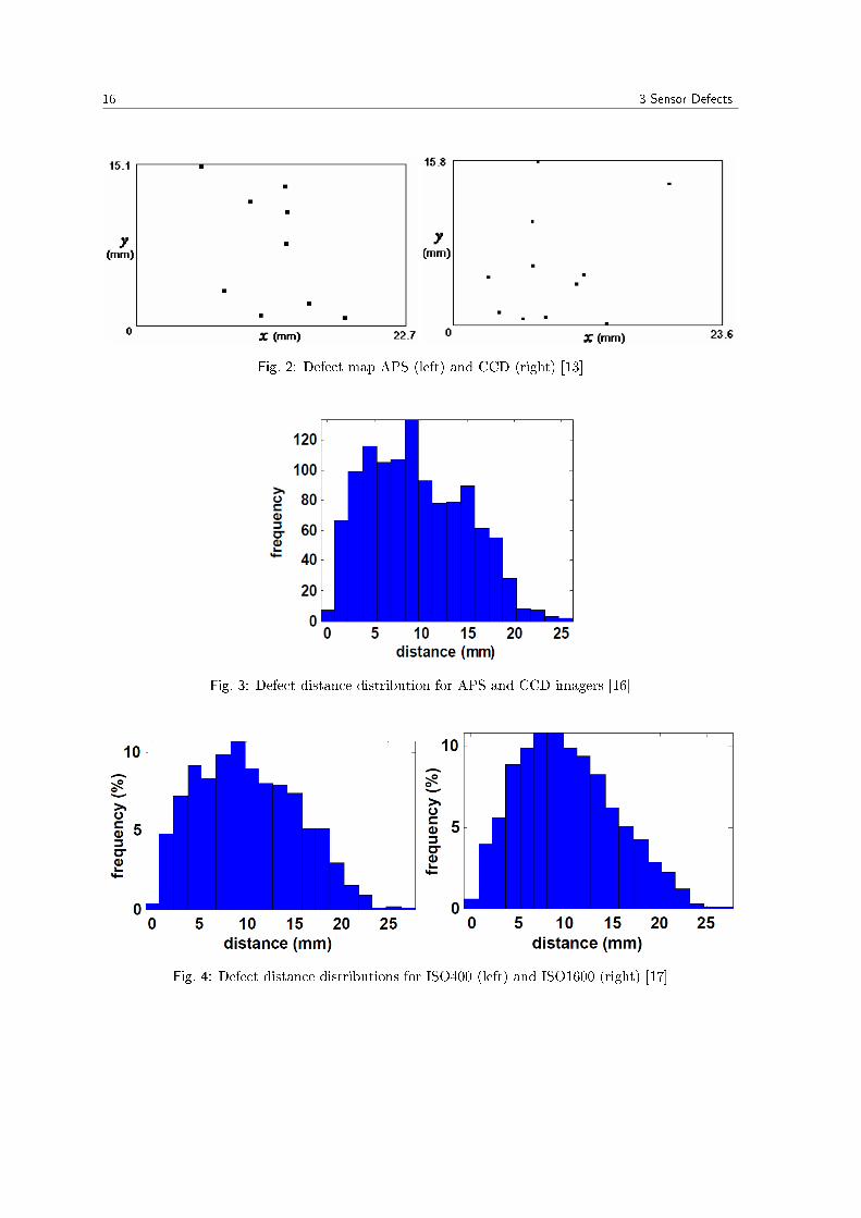
Leung et al. [13, 16] applied statistical analysis to the defect distribution, showing that it is indeeda random distribution. First they used the defect map and inter-defect distance distribution andcompared it with a normal distribution. They showed that there was no signi�cant bias towards shortor long distances [7], which would be the case for defect clustering. This can be seen in the histogramsfor defect distances of APS and CCD image sensors, shown in �gures 3 and 4. This was followed by achi-squared goodness of �t test, which also showed that the hypothesis was correct. In addition theydid a distance to the nearest defective neighbour analysis with subsequent statistical tests (Z-score)and �nally a Monte-Carlo simulation by which they found out that the minimum distance betweentwo defects is 17 µm (at a pixel size of 6-7 µm) [14], inter-defect distances follow a broad distributionand the average distance is 10 mm [13]. This again supports the hypothesis that the defects areindeed randomly distributed. In other words no single event and also no material degradation relatede�ect can be the source causing the defects. They [13] also estimated the size of the defect creatinga hot pixel using statistical methods and found out that it is very small (<0.07 µm [19]/0.2 µm[13]/<0.04 µm [20]) compared to a usual pixel size of 2.2 µm, i.e. the defects are nearly point like,which contributes to the hypothesis that the defects are isolated and not clustered and therefore notcaused by material degradation. As the defects are caused by a point like source, the overall darkcurrent magnitude of the pixel should remain the same independent of the pixel size.
Albert Theuwissen [3] showed that the number of defects is increasing if the camera is exposedto higher cosmic ray radiation (e.g. transatlantic �ights), which is another indicator that the mainsource of the in-�eld defects is cosmic ray radiation. He also found out that the neutrons of the cosmicray radiation are causing these defects.
3.3.2 Temporal Distribution of Defects
Leung et al. [14] analysed the temporal distribution of the defects using two di�erent methods. Firstthey did dark-frame calibrations at regular time intervals (i.e. on a yearly basis) followed by a manualcalibration and second they used an automated defect trace algorithm to determine the point in timewhen the defect �rst occurred. This algorithm works with regular scene images and is described insection 4.4.
If the defects are caused by a causal mechanism, i.e. constant stress to the image sensor, likecosmic ray radiation, the number of defects should increase linearly with time, contrary to a suddenincrease if they were caused by a single traumatic event, like a shock or an exponential increase, i.e.
16 3 Sensor Defects
Fig. 2: Defect map APS (left) and CCD (right) [13]
Fig. 3: Defect distance distribution for APS and CCD imagers [16]
Fig. 4: Defect distance distributions for ISO400 (left) and ISO1600 (right) [17]

3.4 Defect Types 17
Fig. 5: Temporal growth of defects [16]
the time between two consecutive defects gets shorter with increasing age, if they were caused bymaterial degradation, respectively.
They showed that the defects were indeed increasing in number linearly with time, that the defectsare permanent, which means if a defect is there it will not disappear and the defect parameters do notchange over time. They also analysed the inter-defect times, i.e. the timespan between two consecutiveoccurring pixel defects, using statistical methods, which lead to the result that the inter-defect timesare following an exponential distribution. This indicates a constant defect rate which can be modelledby a Poisson process and is in contradiction to material degradation as defect source because thenthe defect rate would increase with time. Another important result is that the sensitivity to defectsdoes not increase with time [7]. Moreover they calculated the defect growth rate for several types ofimagers and Chapman et al. [9] carried on their work by developing a formula showing the in�uenceof the imager properties on the growth rate, which is explained in section 3.7.
3.4 Defect Types
According to the more recent literature there are several defect types which can be distinguished bytheir photoresponse. Table 1 taken from [21] summarizes the most prominent defect types which occureither in-�eld or during the manufacturing process.
3.4.1 Pixel Defect Model (Fridrich)
A pixel model considers the incoming illumination and the impact of pixel defects on the raw outputof the pixel or the sensor, respectively. Jessica Fridrich [18] used the following pixel model:
Y = I + I ◦K + τD + C + Θ
with Y, I,K,D,C,Θ ∈ Rw×h; τ ∈ R and w, h ∈ Z
where Y is the sensor output, i.e. the image, I is the intensity of the incoming light (incidentillumination), I ◦K is the photo-response non-uniformity PRNU, τD the dark current (with τ beinga multiplicative factor taking into account the exposure setting, sensor temperature, ...), C is a light-independent o�set and Θ is some additive modelling noise.

18 3 Sensor Defects
Responsive
to light
Defect type Output function Description
NOStuck high f(x) = 1 Appears as a bright pixel at all the time
Stuck low f(x) = 0 Appears as a dark pixel at all the time
YES
Partially-stuck f(x) = x+ b O�set 0 < b < 1
Hot pixel
(standard)
f(x) = x+Rdark · Texp Illumination independent o�set that
increases linearly with exposure time, i.e.
IdarkHot pixel
(partially-stuck)
f(x) = x+Rdark · Texp + b Has two illumination independet o�sets:(1) increases with exposure time, Rdark
(2) o�set at all the time, b
Tab. 1: Characteristics of di�erent defect types
Fig. 6: Defective pixel example (left: whole image, right: detail of the defect region) [18]

3.4 Defect Types 19
According to this model, a pixel with an extremely high dark current value D is called a hot pixeland is the most common point defect occurring on an image sensor. Another defect type, the stuckpixel, has a high o�set value C. Both pixel defects occur randomly, are uniformly distributed overthe sensor area and are independent from each other. Coming to sensor defects the interesting thingare the two defect matrices D and C, which can be estimated using several images taken by the samesensor. This is done by applying the maximum likelihood method and by working with the noiseresiduals W = Y − F (Y ) = I ◦K + τD + C + I − F (Y ) + Θ, obtained using a denoising �lter F , toimprove the signal-to-noise ratio. As hot and stuck pixels are spiky in nature, a non-linear �lter, likea median �lter is a good choice for extracting the spiky pattern correctly.
Yk, k = 1...d are d images taken from regular scenes at known points in time. Using the noiseresiduals and the pixel model above:
Wk(i) = Ik(i) ◦K(i) + τkD(i) + c(i) + Ξk(i)
with Ξk(i) = Ik(i) − F (Yk(i)) + Θk(i), modelled as an i.i.d. Gaussian sequence with zero meanand variance σ2(i), where k and i are the image and pixel indices, respectively. According to themaximum likelihood principle, the unknown parameter vector Θ = (K,D, c, σ) for a �xed pixel i canbe estimated using (for details see [18]):
θ = argmaxθ
L(W1, ...,Wd|θ)
Simpli�cation of this Model by Bergmüller et. al For this work I adopted the pixel model ofBergmüller et al. [22] which is a simpli�ed version of Jessica Fridrich's pixel model and show that itis similar to the one proposed by Dudas et al. Even if the pixel models of Dudas et al. and JessicaFridrich seem quite di�erent at �rst sight, they are not. Dudas et al. simply do not include the PRNUand the additional modelling noise.
Since all pixels are independent and all operations are done element-wise, the matrix elementsyx,y ∈ Y are denoted as y ∈ Y for simplicity, the same for i ∈ I, k ∈ K, d ∈ D, c ∈ C andθ ∈ Θ. All age independent e�ects can be eliminated since I am interested in the ageing e�ect ofone speci�c sensor, so the PRNU can be eliminated. As I aim for reproducible tests, modelling noiseand environmental in�uences should be minimized, in fact they can be eliminated completely in asimulation, therefore k = θ = 0. For all images taken with the sensor the same exposure settings areused (typically true for �ngerprint, �nger vein and hand vein scanners), therefore τ = const. and τ = 1for simplicity. According to the literature the dark current level is very low for short exposure timeswhich are normally used for standard photographs but also for �ngerprint images to avoid motionblur. Taking all this into account a simpli�ed pixel model can be derived:
y = i+ d+ c with y, i, c, d ∈ R
The most prominent defect types that develop over a sensor's lifetime are hot and stuck pixels. Ifthe dark current d of a pixel is extremely high it is often denoted as hot pixel, whereas if the o�set cis high this results in a saturated pixel and is denoted as a stuck pixel then. As the de�nitions in theliterature are not consistent, Bergmüller et al. [22] de�ned the following model for pixel defects:
y = c
y = i+ d
where the �rst one is light independent and has a constant value c, denoted as stuck pixel andthe second one adds an o�set to the incident illumination and is referred either as partially-stuck or

20 3 Sensor Defects
hot pixel. The cause for hot pixels is a higher dark current at that pixel compared to others. Thedark current level depends on the temperature and exposure time, which are both kept constant inthe experiments, thus the dark current level is constant and therefore there is no di�erence between ahot and a partially-stuck pixel, thus it is simply denoted as hot pixel. This model for stuck pixels canbe directly compared to the one used by Dudas et al. If one takes their hot pixel model (see Equation1), set m = 1 , TExp = 1 , RDark = 0 and set IPixel = y , RPhoto = i and b = d (as discussed before),this reveals the same hot pixel model as it was derived above.
This leads us to the following pixel model for 8 bit grey-scale images:
Y (x, y) =
{C(x, y) if C(x, y) 6= 0
I(x, y) +D(x, y) otherwise
with Y,C, I,D ∈ (Z : [0; 255]w×h)
where C and D are the defect matrices. A pixel's output Y (x, y) saturates at 0 and 255 if intervalborders are exceeded.
This pixel model is the basis for the ageing simulation algorithm, described in section 5.
3.4.2 Pixel Defect Model (Dudas and Leung)
During their �rst experiments, Dudas et al. [12] modelled several defect types using the followingequations, where the output range of a pixel is 0−1 and x = Iphoto ·Tintegration measures the incidentillumination:
fGood(x) = x
fStuck−Low(x) = 0
fStuck−High(x) = 1
fStuck−Mid(x) = c, 0 < c < 1
fPartially−Stuck(x) = x+ b
fAbnormal−Sensitivity(x) = m · x+ b
fHot−Pixel(x) = m · x+ b+ IHotTIntegration
But afterwards they simpli�ed their model to only include hot pixels and partially-stuck hot pixels.They [12, 17] modelled the response I of a pixel using the following equation, which also includes theISO level:
IPixel(Rphoto, RDark, Texp, b) = m · (Rphoto · Texp +RDark · Texp + b) (1)
where Rphoto measures the incident illumination, RDark is the dark current rate, Texp is theexposure time, b is the dark o�set and m is the ampli�cation proportional to the ISO setting.

3.4 Defect Types 21
Fridrich [18] Bergmüller [22] Dudas [12, 17]
IPixel(Rphoto, RDark, Texp, b) =
Model Y = I + I ◦K + τD + C + Θ y = i+ d+ c m · (Rphoto · Texp +RDark · Texp + b)
fStuck−Mid(x) = c, 0 < c < 1
Sensor/Pixel Whole sensor Whole sensor Single pixel
Sensor/Pixel output Y y IPixel
Noise Θ n.a. n.a.
PRNU I ◦K n.a. n.a.
Dark current τD d RDark · TexpIllumination I i Rphoto · TexpHot pixel D >> y = i+ d IPixel = m · (Rphoto · Texp +RDark · Texp)
Stuck pixel C >> y = c fStuck = c, 0 < c < 1
Tab. 2: Comparison of pixel defect models
For an ideal good pixel, both RDark and b are 0 and the output is only proportional to the incidentillumination. A hot pixel now adds a signal on top of the pixel's output, therefore the output of adefective pixel will appear brighter.
As it can be seen, this pixel model only includes hot pixels and partially-stuck hot pixels. Dudas etal. did measurements over the last 7 years and they never found a true stuck pixel, even though theyare discussed in the literature. Moreover they did not �nd any abnormal sensitivity pixels. Insteadthey found partially-stuck hot pixels with a high o�set, appearing as stuck high pixels. Thereforethey use this simple pixel model, which only considers hot and partially-stuck hot pixels. During theirmeasurements [5] they also found out that nearly 80% of the hot pixels are of the partially-stuck type.
3.4.3 Comparison of Defect Models
Table 2 compares the defect models of Jessica Fridrich, Bergmüller et al. and Dudas et al. Pleasenote that some of the entities listed in the table cannot be directly compared, i.e. their units do notmatch, but they are a�ecting the output of the sensor or a single pixel in the same way.
3.4.4 Stuck-High
A stuck high defect is a pixel which output always has the same �xed output value, independent fromthe incoming illumination. A stuck high pixel will appear always bright in the output, i.e. it is stuckon a high value, according to the pixel model above this means the value 1. Dudas and Leung et al.[12, 17] never found a true stuck-high pixel. Instead they found partially-stuck hot pixels with a higho�set (especially if a high ISO settings is chosen) so they suggest that the development of stuck highpixels in the �eld may actually be due to the presence of hot pixels with high o�sets.
3.4.5 Stuck-Low
A stuck low defect is basically the same as a stuck high one, except that its �xed output value is 0,which means this pixel always appears as a dark spot dark in the output image. If cosmic ray radiationis the main source causing the defects and if the mechanisms are like Albert Theuwissen [3, 4, 23]described, then a stuck-low pixel cannot be explained by cosmic ray radiation as source causing thedefects. Defective pixels due to radiation damage can only appear brighter in the output image.
According to Dudas et al. [12], stuck-high and stuck-low pixels are solely factory time defects,which are corrected using factory time mapping. Therefore, they have not found a single stuck defect

22 3 Sensor Defects
Fig. 7: Stuck low and stuck high pixel [11]
during their tests.
3.4.6 Stuck-Mid or Fully-Stuck
A stuck-mid [12] or also called fully-stuck [13] pixel is a generalised form of stuck-high and stuck-lowpixels, which is stuck at an arbitrary but �xed value c in the range 0 ≤ c ≤ 1. Thus a fully-stuckpixel will always have the same output under all illuminations. As with the stuck-low and stuck-highpixels, Dudas and Leung at al. never found a true fully-stuck pixel. A fully-stuck pixel is thereforealso assumed to be a factory time defect, which is corrected by factory mapping.
3.4.7 Partially-Stuck
A partially-stuck pixel has an illumination independent o�set b like a fully stuck one, but also anillumination dependent component. Therefore the output of a partially-stuck pixel is not always thesame under all illuminations. It depends on the exposure time. Again Dudas et al. [12] found outthat all partially-stuck defects that they described earlier were actually also hot pixels, which suggeststhat a common mechanism may lead to both defects.
3.4.8 Abnormal Sensitivity
There are basically two types of abnormal sensitivity pixels, low sensitivity ones, showing only afraction of their incident illumination and high sensitivity ones, showing more than the correspondingincident illumination on the output. This type of defect is identi�ed by comparing the illuminationresponse of the pixel with its neighbours. As the neighbouring pixels should have the same sensitivity,variations in sensitivity indicate the presence of an abnormal sensitivity pixel defect. Once moreDudas et al. [13, 12] never found an abnormal sensitivity defect.
3.4.9 Hot Pixel
A hot pixel is a defect that has an illumination independent component which increases linearly withexposure time. Whereas the dark response of a good pixel should be close to 0 (due to sensor noiseit is not exactly 0), the dark response of a hot pixel increases with the exposure time. The output ofa hot pixel is di�erent from noise and it appears as a bright spot with a �xed location in the outputimage. The added dark response limits the light collection capacity of the pixel, causing it to saturateat a lower illumination level, which reduces the pixel's dynamic range. As a hot pixel results fromnon-light generated charge at the pixel, i.e. an increased dark current, it is also called gain enhanced

3.4 Defect Types 23
Fig. 8: Abnormal sensitivity pixel [11]
Fig. 9: Hot pixel response [15]
defect. According to Leung et al. [17], the majority of hot pixel defects found in larger sensor areaDSLRs are low impact defects with a low dark current level. Therefore, these defects are almostinvisible in images captured under normal conditions (short exposure time and low ISO level) andhave only little in�uence on the image quality.
A typical method to compensate hot pixels used by many camera manufacturers is to capture adark frame of the same exposure time right after the image is captured and subtract this one fromthe original image, which should eliminate the dark signal then. An interesting fact is that hot pixelsbecome more visible if many images are captured in rapid succession while the response of good pixelsremains the same. This might be due to heating of the image sensor, which leads to an increased darkcurrent and therefore a higher hot pixel amplitude. Thus the automatic detection of hot pixels getseven more challenging because of the varying dark signal and therefore varying hot pixel amplitude.

24 3 Sensor Defects
3.4.10 Partially-Stuck Hot Pixel
The literature is not completely clear about how to name this defect. According to Leung et al.[14], a partially stuck hot pixel has an additional component (o�set) that is independent from theillumination and exposure time. Therefore, it can even be observed at no exposure (0 exposure time)and will in general appear brighter than a standard hot pixel. Thus it has a higher impact on theimage quality because the pixel goes into saturation at a lower illumination level, which further reducesthe dynamic range of the pixel. In addition partially-stuck hot pixels cannot be compensated by thesimple method described above for standard hot pixels, because if the combined illumination and darksignal causes the pixel to saturate, just by subtracting the dark response will not recover the originalsignal. Jessica Fridrich [18] does not explicitly mention partially stuck hot pixels.
3.5 Defects in Colour Images
Unless images are captured in RAW mode, several imaging functions are applied to the output imagescaptured in colour mode, which is the usual mode used in photography. These imaging functionsinclude demosaicing, noise reduction, white balance etc. Although they are intended to improve theimage quality, they ignore the presence of defects, i.e. defective pixels are treated as good ones, so theymight not only amplify but also spread the impact of a defective pixel to its neighbouring good pixels.Especially demosaicing, which is the �rst function applied in the imaging pipeline, has a signi�cantimpact on the appearance of defective pixels. It is needed for every CFA image sensor to recover themissing two colour channels at each pixel. This is done by interpolation using the neighbouring pixelsbut ignoring the presence of defects, which will lead to incorrect interpolation values. Depending onthe type of interpolation used, it will distort the defective pixel, causing a singe defect to appear asa virtual cluster. Such a defect cluster is more visible than a single pixel defect. Thus sensor defectsare highly undesirable in colour images. Nowadays the most widely used demosaicing algorithms areadaptive ones, taking the characteristics of the image into account, similar to the Kimmel algorithm,which reduces the Moire pattern. But these more advanced demosaicing algorithms also have a higherimpact on the defect appearance compared to simple bilinear interpolation and may even spreaddefects into other colour channels. To be able to detect the defect location, each local cluster isconsidered as one defective pixel and the peak of the defect cluster appearing in the output image isused as defect location.
Most cameras use JPEG compression for colour images. This compression reduces the peak error,but may spread a single defective pixel or a virtual defect cluster even wider, which of course has anegative e�ect on the output image. JPEG compression also suppresses colour variations of all thethree colour planes which lowers the impact of the defective pixels.
All these imaging functions applied to colour images have an irreversible impact on the pixel defectsin colour images, in the way that they further degrade the quality of output images and make thedetermination of the exact defect location more di�cult, but the defect itself may be easier to detectbecause its higher impact. Therefore, a suitable defect detection algorithm has to be adopted to beable to handle colour images correctly.
3.6 Defect Identi�cation Techniques
There are di�erent techniques which can be used to identify the di�erent types of defective pixels.With DSLR cameras all of these techniques can be used, because these cameras do not only providethe RAW format, but also manual control of camera parameters, especially exposure control. If PS(point-and-shoot) or mobile phone cameras should be investigated some of these techniques cannotbe used at all or have to be adopted.

3.6 Defect Identi�cation Techniques 25
Fig. 10: Defect cluster after demosaicing [14]
Fig. 11: Red hot pixel in RAW image (left) and after processing (right) (from: http://www.
pixelfixer.org/faq.html)
3.6.1 Dark Field Calibration
The dark �eld calibration can be used to identify stuck-high, fully-stuck, hot and partially-stuck hotpixels. Standard dark �eld calibration uses a dark �eld exposure, i.e. taking an image with no incidentillumination. Therefore the output image should be completely black and a stuck high or hot pixelwould appear as bright dot. Dark �eld calibration can be easily done even with digital cameras nothaving a shutter. A stuck high or a hot pixel's location can be identi�ed using a simple threshold testto distinguish a sensor defect from random noise, e.g. if the output of the suspect pixel is 3 timeshigher than the noise signal it is declared as defective. Figure 12 shows an example of a dark �eldcalibration image.
The distinction between stuck high and hot pixels can be made by capturing several dark �eldimages with increasing exposure times. According to the pixel model of Leung et al. [13, 14], a hotpixel has an illumination-independent component that increases linearly with exposure time, so it willappear brighter if the exposure time is increased, while a stuck pixel does not change its intensityvalue.
The dark response Ioffset of a hot pixel, also called combined dark o�set, can be estimated bysetting Rphoto = 0 in the pixel model (section 3.4.2), then it becomes
Ioffset(RDark, Texp, b) = m · (RDark · Texp + b)
which is independent of the incident illumination. A linear function can be used to estimate thedefect parameters RDark (slope of the pixel's response) and b (o�set along the y-axis of the pixel'sresponse), see �gure 9 for details. For a standard hot pixel b = 0 while for a partially-stuck hot pixelan additional, illumination and exposure independent o�set is added and b 6= 0. Standard hot pixels

26 3 Sensor Defects
Fig. 12: Dark �eld capture example [18]
are most visible in images taken with long exposure times, while partially-stuck ones are visible in allimages depending on the o�set value b. The hot pixels are then identi�ed using a threshold test toeliminate sensor noise.
3.6.2 Bright Field Calibration
Similar to the dark �eld calibration, in bright �eld calibration a bright �eld exposure is used. Thistechnique can be used to identify stuck-low defects and also fully-stuck defects. Dudas et al. [12]capture an image with uniform illumination near saturation. In the output image all good pixelsshould have the same intensity value, whereas stuck low pixels would appear darker. Like in a dark�eld image, also here the pixel defects can be detected using a simple threshold test. According toLeung et al. [16] they never found a single stuck low pixel (except for manufacturing time defectswhich are normally masked out). Jessica Fridrich [18] suggests to capture an image of a partlycloudy sky instead. In such an image also stuck high pixels are visible if they are stuck on a veryhigh value near saturation. Especially for bright �eld calibration a set of calibrated equipment isnecessary to reproduce a uniform illumination at a known intensity, which is necessary to estimatethe defect parameters in addition to the defect location. So the complexity and high costs makethese defect detection method impractical for in-�eld use and thus it is typically used by image sensormanufacturers only.
3.6.3 Defect Identi�cation for PS and Cellphone Cameras
Leung et al. [14] pointed out that the dark �eld calibration procedure as described above cannotbe used for PS and mobile phone cameras due to the limited exposure control. In fact the cameraexposure system has to be tricked to give maximum exposure time, which is necessary to be able to doa dark frame calibration at all, but there is no ability to use increasing exposure times. Thus it cannotbe distinguished between a stuck-high and a hot pixel. Moreover these cameras do not provide the

3.7 Impact of Sensor Parameters on Defect Growth Rate 27
RAW format, therefore the calibration images are captured in colour mode. As described in section3.5, in colour mode several imaging functions are applied (main problem is the colour demosaicing),therefore a single defect will appear as a virtual cluster. Thus each local cluster has to be consideredas one defective pixel using its peak output as the defect location. Each time they captured a seriesof 3 images and used the common result to eliminate false detection due to noise.
Another problem regarding mobile phone cameras is that for cost reasons there is no factorycalibration done. Therefore it cannot be distinguished between factory time and in-�eld defects at the�rst measurement (initial number of defects may include factory time defects) but only on subsequentmeasurements. This is also the reason why there might not only be hot pixel defects but also stuckand low sensitivity pixel defects found across these types of cameras.
3.7 Impact of Sensor Parameters on Defect Growth Rate
Chapman et al. [9, 6, 7] showed by continued empirical measurements of several imagers with di�erentcharacteristics (DSLRs, PS cameras and mobile phone cameras) that the rate of newly generated pixeldefects depends on the sensor technology (CCD or APS) and on sensor design parameters like sensorarea, pixel size and gain (which is adjusted using the ISO value), pointing out important trends indefect development. They showed that the defect rates scale linearly with the sensor area, so theyintroduced a metric called defect density measured in defects/year/mm². The dependence of thedefect density on pixel size and ISO is not linear. Instead they found the best �t by using a powerlaw relationship, according to:
D = A · SB · ISOC (2)
where D is the defect density (defects/year/mm²), A is the number of defects/year/mm² if the pixelsize is 1µm, S is the pixel size in µm, ISO is the ISO level and B and C are constants dependingon the sensor type. For a CCD sensor A = 0.0141, B = −2.25 and C = 0.69 and for an APS sensorA = 0.0742, B = −3.07 and C = 0.5.
3.7.1 Sensor Type
In general, CCD sensors tend to have a higher defect count than APS ones of the same age (∼ 3xhigher than APS for DSLR sensors with the same size at all ISO levels). If cosmic ray radiationis the main source of the defects, then an explanation why CCD sensors are more sensitive to thedevelopment of in-�eld defects is that on the one hand the size of a CCD sensor pixel is 2x largerthan the size of an APS pixel and on the other hand CCD sensors have a higher �ll factor (70-90%)than APS sensors (∼ 25 − 30%). This means that at the same pixel size, the photosensitive area ofeach pixel is only about 25% for an APS sensor compared to about 80% for an CCD sensor. As thephotosensitive area increases and because the cosmic ray total �ux is constant per area, the defectrate is also increased.
But this is only true for pixel sizes of about 6 − 7µm. For a pixel size of 2.1µm, APS and CCDsensors would have the same defect density. For even smaller pixels, APS sensors would have a higherdefect rate than CCD ones. This means that CCD pixels are not as sensitive to a shrinkage in pixelsize as APS ones, which can also be seen from the value of B in the formula. The impact of the pixelsize on the defect density is described below.
3.7.2 Sensor Area
The linear increase in the defect density with increasing sensor area can also be explained based oncosmic ray radiation as the main source causing the defects. According to [3, 4] the cosmic ray total�ux per area is a random process with only minimal changes over time in a given location, i.e. it

28 3 Sensor Defects
scales with the area and therefore a larger photosensitive area increases the exposure to the radiation.But the defect rate only scales linearly with the area if the pixel size remains the same. Otherwisethe change in the defect density also depends on the change in pixel size as described below.
3.7.3 Pixel Size
The pixel size has a high impact on the defect density. In the last few years the sensor sizes haveremained the same, but the number of pixels increased. This can only be achieved by reducing thepixel size. Especially sensors equipped in mobile phones have very small pixel sizes (side length of 1-2µm). If the pixel size would have no impact, one would expect the sensor with the highest area todevelop the most defects if the pixel size is kept constant. But instead the expected rate from scalingup the defect rates of PS and cellphone cameras by the sensor area is much higher than the observedrates for the DSLRs. As the equation 2 shows, the defect density increases rapidly with decreasingpixel size. It scales approximately inverse linear with the pixel area for CCD sensors and much morethan inverse linear with the pixel area for APS sensors, which means that sensors with smaller pixelsare more sensitive to developing defects. As the relationship between pixel size and defect rate isexponential, the impact of reducing the pixel size is much higher than increasing the sensor size. Asmost of the smaller sensors are APS ones, this has a great impact on the quality of the output images.If the pixel size shrinks down to 1 µm the increasing defect rate will require a signi�cant amount ofdefect suppression and even the usual mapping done by the manufacturers to ignore the output ofhot pixels and replace their values by interpolation from other pixels may fail as a defect correctionstrategy.
According to Chapman et al. [5] one reason for this much higher defect rate might be that dueto the smaller area per pixel only a smaller fraction of the incoming light (about 10% compared toDSLRs) is collected. Therefore to create a similar output, the scaling factor m in the pixel modelhas to be increased. This is similar to increasing the ISO level as described below, therefore also theimpact of the defects, especially IOffset increases. This means that hot pixels which would have a lowin�uence on a sensor having a larger pixel size are much more visible at this small pixel size. Anotherreason is that the dark current of a hot pixel, which is caused by the defect source, remains the sameas the pixel size shrinks, but the sensitivity of the pixel to each electron increases and therefore evena small hot pixel damage will cause a signi�cant e�ect on a smaller pixel. Currently the reason forthe di�erence in sensitivity between CCD and APS sensors if it comes to pixel size is not completelyclear and needs to be explored.
3.7.4 ISO Level
In previous times the usable ISO range was limited by the sensor noise. But as sensors got better,the noise level decreased and in addition noise suppression algorithms are utilized, pushing the usableISO ranges for modern DSLR cameras up to 25600 now. Capturing images at high ISO levels enablesnatural light photography without the need for a �ash or resorting to long exposure times which isa great bene�t for photographers. But unfortunately the pixel defects are increasing in their numberwith higher ISO values. Leung et al. [17] showed this by performing the dark frame calibration atvarious ISO levels. The reason is that the ISO setting is nothing else than a numerical gain (see thepixel model in equation 1), thus also the defect parameters (o�set and dark current) are ampli�ed(scaling linearly with the ISO level), enhancing the brightness of a hot pixel. As the o�set is ampli�ed,partially-stuck hot pixels are going into saturation even at short exposure times, making them appearlike a stuck high defect. This is also a major drawback for the pixel's operation, because this higho�set reduces the dynamic range of the pixel. Of course the threshold for determining a defect alsohas to be increased as the sensor noise increases. But the brightness of the defects increases at amuch higher rate than the background noise signal, therefore at higher ISO levels more defects can be

3.7 Impact of Sensor Parameters on Defect Growth Rate 29
Fig. 13: Dark response at various ISO levels [9]
found, because they are more distinguishable from the noise. Leung et al. [19] noticed a substantialincrease in the number of defects detected at ISO 3200 compared to ISO 100. The reason for thisincrease is that many of the defects are barely visible at lower ISO settings due to low RDark and bvalues, i.e. they cannot be distinguished from the noise signal, so they may not pass the thresholdtest. The defects present at higher ISO levels a�ect a wider range of exposure times and are visibleeven at short exposure times (due to their high o�set). According to the quantitative values, CCDsensors are more sensitive to an increase in the ISO level than the APS ones.

30 3 Sensor Defects

31
4 Defect Detection Algorithm
Each image is a snapshot of the sensor's state at a given time, i.e. of all of its pixels, including thedefective ones. As described above, defects are usually detected using special calibration images (darkand bright �eld exposure). Unfortunately such images were not available for the type of �ngerprint,�nger vein and hand vein sensors utilised to capture the databases I worked with during my evaluations.Using calibration images the incident illumination is uniform and known, therefore the defects canbe easily detected and their parameters can be estimated. If only �ngerprint, �nger- or hand veinimages, respectively, captured by a speci�c sensor are available, the illumination is neither uniformnor known. Moreover, factors like the ISO level, exposure time and the complexity of the image scenewill a�ect the visibility of the defects. In this case, some kind of statistical approach using a sequenceof images has to be used to identify the defects.
Of course all of the methods described below are only heuristics and will never achieve an accuracyof 100%, i.e. identify each defect correctly. Thus the number of defects and their parameters detectedby these methods can only be an approximation of the real values. The majority of photographsare taken at short exposure times (∼ 1/30 s) and low ISO settings (<ISO800) [17], thus low impactdefects, especially hot pixels with a low dark current magnitude, are barely visible in these imagesand might not be detected at all. Long exposure times are not used often, because camera motionwill cause blur in the image unless a tripod is used.
The EXIF data provides additional information (exposure time, ISO setting, capture date), whichcan be used to estimate the parameters of the defects (dark current amplitude, o�set, etc.) butunfortunately this information is not available for most �ngerprint, �nger vein and hand vein images,because these are usually stored in lossless formats like Bitmap (bmp), Portable Network Graphics(png) or TIFF which do not contain EXIF data.
4.1 Filters for Defect Identi�cation
Sensor ageing related defects occur in the form of single pixel, point like defects as discussed above.Therefore �lters like median, ring averaging and 4NN and 8NN minimum distance are suitable todetect the defects. The image is �ltered, then the actual pixel value is compared with the one in the�ltered image. The probability for the centre pixel to be defective corresponds to the di�erence of thepixel values.
4.1.1 Median Filter
The median �lter is de�ned by:
y(i, j) = median(m,n)∈G(i,j)
{I(m,n)}
where the pixel (i, j) is the centre pixel which is under examination, y(i, j) is the output of the�lter, G(i, j) denotes the locations of pixels within a neighbourhood around the centre pixel. This canbe any type of neighbourhood. I(m,n) are the outputs of the neighbouring pixels.
4.1.2 n× n Ring Averaging Filter
In contrast to the standard averaging �lter, which takes the average of all the pixels inside a squareor rectangular neighbourhood around the centre pixel, this �lter only takes the average of all pixelsinside a ring, centred at the centre pixel as output value. This mitigates the e�ect of defect spreadingdue to colour demosaicing, which mostly a�ects pixels directly neighbouring the defective centre pixel,as only pixels on an outer ring are considered for the calculation of the interpolation value.

32 4 Defect Detection Algorithm
Fig. 14: n× n ring averaging �lter [16]
Fig. 15: 4NN �lter [16]
4.1.3 4NN Filter
This �lter basically takes the mean of the centre pixel's north, south, east and west neighbour asoutput value.
4.1.4 4NN and 8NN Minimum Distance Filter
The minimum neighbouring pixel di�erence �lter can be de�ned by:
y(i, j) = min(m,n)∈G(i,j)
{|I(i, j)− I(m,n)|}
where the pixel (i, j) is the centre pixel which is under examination, G(i, j) denotes the locations ofpixels within a neighbourhood around the centre pixel. This can be an 8 neighbourhood (3x3 windowcentred at the pixel and using all pixels without the centre one) or a 4 neighbourhood (using onlythe pixel directly south, north, west and east of the centre one) or any other type of neighbourhood.I(i, j) is the output of the centre pixel and I(m,n) are the outputs of the neighbouring pixels.
4.2 Thresholding Based Approach
This is a two step approach. At �rst the stuck pixels are identi�ed using the same property as inthe statistical approach proposed by Bergmüller et. al [22], which is described below, but no hardcomparison (a stuck pixel is supposed to have exactly the same value in all images) is used. Instead acertain threshold can be set (in percent of the maximum pixel value) to account for sensor, analog todigital conversion and transmission noise, respectively, which means a stuck pixel might not always

4.3 Statistical Approach 33
have exactly the same pixel value. The second threshold de�nes in how many images (also in percentof the total number of images) the pixel must have the same value within the tolerance to be identi�edas stuck pixel.
In [24] a pixel is identi�ed as low sensitivity pixel if:
|∑Nk=1 P (k)
N− P (0)| ≥ C, C = 10%
where P (k) describes the value (output) of a pixel, the pixels k = 1...N describing a neighbourhood(e.g. window centred at the pixel) around the pixel and P (0) is the output of the centre pixel. C = 10%means 10% of the maximum possible output value of a pixel. A pixel is identi�ed as stuck low, i.e. ithas a value of 0 if:
|∑Nk=1 P (k)
N| ≥ C011
P (0) ≤ C012
where C011 and C012 are 50% and 10% of the maximum possible output value of a pixel, re-spectively. This means that a pixel is only identi�ed as stuck low if it has a value near zero and itsneighbouring pixels have a value greater than or equal to127 (for 8 bit images) on average. A pixel isidenti�ed as stuck high if:
|∑Nk=1 P (k)
N| ≤ C101
P (0) ≥ C102
where C101 and C102 are 90% and 50% of the maximum pixel value, respectively. This means thatsimilar to stuck low pixels, a pixel is only identi�ed as stuck high if its value is near the maximumvalue and its neighbouring pixel values are below or equal to 127 on average. Of course the thresholdvalues C can be adjusted according to the input images. In the original paper only a single image isused, not an image sequence. This approach was also tested for the implementation with an imagesequence but did not improve the result, so the simple method using the two thresholds was used.
The next step is the identi�cation of the hot pixels. A hot pixel is a point defect, i.e. a single pixel,which appears brighter than its neighbouring pixels, so it can be identi�ed by comparing the pixel'svalue to the value of its neighbouring pixels. Therefore, the �lters described above can be used togenerate an interpolation (prediction) image and compare the prediction with the actual pixel valuethen. If the error is above a certain threshold, the pixel is identi�ed as hot pixel in the current imageand again if this pixel is identi�ed as hot one in a certain percentage of all images (above the secondthreshold) it is �nally identi�ed as hot pixel. This approach is only able to estimate the number ofhot pixels but not their parameters.
4.3 Statistical Approach
This approach was proposed by Bergmüller et. al [22] to estimate the defect growth rates and amp-litudes using two image sets, taken with the same sensor at di�erent points in time. Y0...YK is asequence of K images taken in a very short period of time. A stuck pixel has the same value in eachimage of this sequence, therefore a pixel at a given position is stuck if:
y0 = y1 = ... = yK

34 4 Defect Detection Algorithm
A partially stuck pixel1 at position (x, y) adds a light independent o�set to the pixel's output atthat position yk = Yk(x, y). First the pixel's mean y is computed from the whole image sequence.The mean is then substituted using the pixel model from section 3.4.1. Because stuck pixels can bedetected using the above method, the possibility of a pixel being stuck can be ruled out, thus c is notconsidered here. To take impredictable impacts during acquisition into account, some modelling noiseis added, leading to the following equations:
y =1
K
K∑k=1
yk
y =1
K
K∑k=1
(ik + d+ θk)
If K is su�ciently large, the mean of a uniformly distributed modelling noise θ cancels out. Underthe assumption that there are no pixel defects present, the o�set d = 0 which is denoted as d′. Underthis assumption ik = yk can be substituted and the pixel's mean y is denoted as y′. The partially-stuck (I denote it as hot pixels) defect matrix d contributes to each pixel's output uniformly, thusit is independent of k. If there are no pixel defects and if the pixel means y mostly have identicalvalues in a q × q neighbourhood, the identity y′ ≡ median(y, q) holds. This is the case if only pixelmeans of image regions with mostly uniform brightness and texture, e.g.. outside the �nger area in�ngerprint images, are considered. Thus regions covered by the �nger area have to be masked out(Bergmüller et al. [22] originally masked out the area where the iris texture is). As the defects aredistributed uniformly across the sensor area (i.e. inside the image) it is su�cient to use only a certainpart of the image, search for defects in this area and derive the total number of defects inside thewhole image based on the percentage of the whole image area which is covered by the part used tosearch for defects.
Sparse outliers within the q × q region are �ltered out due to the non-linear nature of the median�lter. Such outliers occur if there is a pixel defect. Thus the median is able to compute a pixel'smean y′ disregarding the in�uence of pixel defects. Using this relation, y′ → median(y, q) is set and
thus d′ → d can be used as an estimator for the o�set, which is added to the incident illumination ik,leading to the pixel's output yk.
y′ = d′ +1
K
K∑k=1
(yk)
d =1
K
K∑k=1
yk −median(y, q)
Not only information about the partially-stuck pixels but also information about the PRNU iscontained in d. The PRNU is likely to be normally distributed, therefore the size of the median kernelq has to be chosen large enough to minimize this in�uence on the median(y, q), which is the case if anormal distribution in the logarithmic histogram is observed inside the q× q neighbourhood, like it isthe case for the whole image.
A pixel is identi�ed as partially-stuck if d is an outlier with respect to the normal distribution,i.e. it has a much higher sensitivity than expected from the PRNU. This is done using a decisionthreshold d > τps which is chosen manually.
1 It is usually denoted as hot pixel during this thesis. But to comply with their original explanation it is calledpartially stuck pixel in the following.

4.4 Bayesian Inference Based Approach (Dudas) 35
4.4 Bayesian Inference Based Approach (Dudas)
This is another statistical approach but in contrast to the one above it uses Bayesian inferences tocalculate the probability of each state for each pixel separately from a series of images taken by thesensor within a short timespan. It is based on the defect model described in section 3.4.2, whichmodels an imager as an array of W ×H pixels where the illumination present at a pixel at position(i, j) is denoted as xi,j . The output (response) of each pixel is denoted as yi,j , is in the range of [0, 1]and can be written as a linear function of the incident illumination:
yi,j = mi,j · xi,j + bi,j
where the subscripts are omitted for simplicity. m is the sensitivity or gain and b is the bias oro�set, both having characteristic values for speci�c defect types (see pixel model in section 3.4.2). Anideal, non-defective pixel would have m = 1 and b = 0. Each defect type can therefore be described bya combination of gain m and o�set b and is referred as D = (m, b). A stuck high pixel can be describedby (0, 1) and a stuck low one by (0, 0). The probability of the occurrence of a speci�c defect type(m, b) is denoted as p(m,b) and the total probability of any defect occurring, i.e. the defect density,can be calculated by ptotal =
∑{D} p(m,b). To completely calibrate an image sensor, the parameters
m and b, i.e. the sensitivity and bias of each pixel has to be determined.As the defects cannot be reliably determined solely based on one image, a sequence of images
has to be used. These are images captured in the �eld under normal operation conditions which areanalysed and the statistics of each image and defect type are accumulated using Bayesian inferences.The details of the algorithm are described in [10, 11]. After capturing T + 1 images the samples
Y = y(0)i,j , y
(1)i,j , ..., y
(T )i,j from a speci�c pixel at position (i, j) are available. Using Bayesian inferences
the probability of each defect type D at each pixel position (i, j) can be estimated based on thecollected evidence (image samples) using (subscripts are omitted for simplicity):
P (D|Y = y(0), y(1), ..., y(T )) =P (Y |D) · P (D)∑
D′={allD}P (Y |D′) · P (D′)
where the conditional probability P (Y |D) is the most important term, which encapsulates theprobability of observing the data Y under the assumption that the given defect type D is present atthat pixel. This likelihood has to be evaluated within the context of the image being processed. TheBayesian function accumulates the statistics over a sequence of images to estimate the probability ofa pixel to be of a certain defect type D. There are two schemes for the evaluation of this data basedon statistical metrics calculated from the image, which are described in the following subsections.P (D) denotes prior knowledge of the occurrence probability of each defect type and can be obtainedfrom manufacturing test data. These calculations are done recursively, such that each image in thesequence is processed individually. The previous iterations lead to the a priori probability at iterationk. This is expressed by the following formula for the k-th iteration:
P (D|Y = y(0), y(1), ..., y(k)) =P (y(k)|D) · P (D|y(0), y(1), ..., y(k−1))∑
D′={allD}P (y(k)|D′) · P (D′|y(0), y(1), ..., y(k−1))
This conditional likelihood term is evaluated for the whole sequence of T images and after that, thedefect type with the highest likelihood at a given pixel is taken as resulting defect type. Of course theset of all defect types should also include good pixels to be complete. The parameter T is set beforethe testing begins. T should not simply be chosen to use all available images, because long sequencesmay cause the statistics to saturate. Other termination criteria, like a pre-determined con�dence

36 4 Defect Detection Algorithm
level, i.e. likelihood threshold are also possible. Then the convergence speed is strongly a�ected bythe content of the images in the sequence. A �owchart of this approach is shown in �gure 17.
Especially if not only the defect location but also the earliest date in time where the defect showedup should be determined (which can be done if the image sequence covers a longer timespan), a slidingwindow approach should be used, at which only the n most recent images are used to calculate theaccumulation. According to Leung et al. [15], a window length of 3 is best for accurate temporaldetection of low visibility defects. For an accurate detection of the date when the defect occurred�rst in time, a dark-frame calibration image is essential, from which the �rst prior probabilities P (D)for each pixel and defect type can be derived. Changes in the accumulated probability indicate thepresence or absence of defects. Therefore, the date when a pixel �rst got defective can be eitherdetermined using a simple threshold test, i.e. if P (Good|y(x)) falls below a certain threshold or usinga probability ratio threshold test: P (Good|y(x))/P (Good|y(k−1)) > threshold.
A problem regarding this approach might occur if only a certain type of images, e.g. landscapescenes with large black and underexposed areas are used. Then defects like stuck low pixels cannot bedetected. In �ngerprint images where the outer image regions are rather bright all the time, defectslike hot pixels might remain undetected if their amplitude is rather low. Finger-vein images are usuallydark grey to black outside the �nger region, consequently the detection of stuck low pixels may notbe possible. Also hand vein images may exhibit such low brightness regions if not only a ROI butthe whole image of the hand including the surrounding areas is used. According to Dudas et al. [12]this method can only be used to detect hot pixels if images with su�ciently long exposure times areavailable.
4.4.1 Image Statistics Method
This technique relies on image wide statistics to derive the probability for each defect type and istherefore called image statistics method [25]. It relies on the image-wide distribution of pixel values inthe form of the density function PX(x), which is estimated for each image using the image histogramPY (y). E.g. the likelihood P (y(k)|D) for a pixel to be stuck at a value c simply is:
P (y(k)|D(0, c)) =
{1 y(k) = c
0 otherwise
and for a pixel with half sensitivity it is:
P (y(k)|D(0.5, 0)) = PX(2y(k))
The problem of this simple approach is that a stuck pixel might not always have the same outputdue to noise. Thus the conditional probability models have to be adjusted in a way that the statist-ical distributions do not represent a single impulse function but a smooth function, like a Gaussiandistribution with its mean value at the stuck pixel value and a small variance. The likelihood fora pixel being good is given by P (y(k)|D(1, 0)) = PX(y(k)). If the output for a speci�c defect typegives unlikely values after testing many images, that defect type is not very likely to be present atthat pixel. Therefore, pixels that are consistently having an output of 0 or 1 are not very likely to begood, because these extreme values are not likely to occur very often in typical images. But if onlyglobal information is used and local information around the pixel of interest is not taken into account,this may lead to false identi�cations depending on the images contained in the sequence. E.g. in thecontext of �ngerprint images the outer region might always be rather bright depending on the type ofsensor, which might lead to the false identi�cation of stuck high pixels. Finger- and hand vein imagesshow rather large bright parts and only little dark parts where the veins actually are. Outside thehand or �nger region there are some quite dark parts. This may lead to both, the false detection of

4.4 Bayesian Inference Based Approach (Dudas) 37
stuck-low and stuck-high pixels inside the respective parts. If the information of neighbouring pixelsis additionally used, these false identi�cations can be avoided, because it is unlikely that not only asingle pixel is stuck high but also all of its neighbours are. In a photograph saturated white areasare undesirable, therefore the dynamic range of the image is limited by the image processing chainof many cameras, which could a�ect the image statistics PX(x) and PY (y) in undesirable ways. Thisleads us to the interpolation technique which is described next.
4.4.2 Interpolation Method
The more successful technique for calculating P (Y |D) or P (y(k)|D), respectively uses informationfrom the pixel's neighbourhood. The details of this approach are described in [11]. The output ofeach pixel is compared to its neighbours and the probability that this pixel is faulty is calculated,assuming that most of the pixels in the neighbourhood of a defective pixel are good ones. This isdone by �rst estimating the incident illumination at the pixel's location (i, j) by interpolating itsneighbouring pixels' values. Of course the choice of the interpolation scheme has a signi�cant impacton the accuracy of the detection method. Although several interpolation schemes can be used, for thisapplication the emphasis is placed on di�erent performance parameters than for typical applications.E.g. many schemes try to maintain high-frequency components in the output and try to use as muchof the surrounding data as possible, which is both contra productive for defect detection. The authorsproposed the 4NN and ring averaging schemes, which are shown in the �gure 16. The smaller theinterpolation region and the closer this region is located towards the pixel under investigation, thebetter will be the estimate of the pixel's value. According to Jenny Leung [21], the 5x5 ring averaging�lter provides the best tradeo� between accurate pixel estimation and avoiding the defect spreadingproblem caused by colour interpolation if dealing with colour images. If the estimated pixel valueat position (i, j) is denoted as zi,j , then the estimation error can be calculated by ei,j = zi,j − yi,jfor each pixel in the image. Based on the estimation error, the estimation error density PDF pE(e)is calculated over the whole image and its statistics are accumulated in the probability distribution(CDF) PE(e), which also describes the e�ectiveness of the estimation scheme. Now the likelihood foreach defect type can be determined by calculating the expected error eD at each pixel, for each defecttype D and retrieving the probability for this defect type from the distribution PE(eD) using
P (y(k)|D) = PE(e(k)D = fD(z)− y(k))
P (y(k)|(m, b)) = PE(e(k)D = z − [
y(k)
m− b])
where fD describes the transfer function of the defect type. E.g. a pixel stuck at value c has
P (y(k)|D(0, c)) =
{1 y(k) = c
0 otherwiseand a a half sensitivity pixel has P (y(k)|D(0.5, 0)) = PE(z − 2 · y).
Like before, the predicted defect type at the pixel (i, j) is the one with the highest likelihood then.The estimate from the interpolation does not need to precisely predict xi,j at each image, becauseusing a certain number of test images, the results should be reasonably accurate. Thus this schemeis more e�ective than the image statistics method. The authors claim that only 50 ordinary imagesare su�cient to accurately identify all faults without falsely diagnosing good pixels as faulty [11].They also found out that the 8NN or 3x3 averaging �lter work better than the 4NN averaging �lterbecause due to the smaller weighting of each single pixel defects have less impact on the interpolationresults. Furthermore adding noise only slows down convergence rates but does not a�ect the falsepositive detections. Using other interpolation schemes like the 4 round-robin technique, which is amodi�cation of the 4NN scheme and described in [10] further mitigates the e�ects of a catastrophic

38 4 Defect Detection Algorithm
Fig. 16: Filters for interpolation method [15]
error but might be less accurate. It basically splits the 4NN interpolation into 4 separate tests anduses a majority voting scheme. At �rst the pixel is compared to its left neighbour and the probabilityP (D|y(k)) is evaluated, then it is compared to the neighbour above, again evaluating the probabilityusing the left pixel's test probability as prior probability. This is continued until all 4 neighbourshave been examined. If the interpolation error becomes very large this causes issues within theBayesian statistical methods (saturation), which leads to false positive detections and should thereforebe avoided.
As mentioned before if only colour images are available for defect detection, the single pixel defectsare distorted by the multiple steps in the image processing chain of the camera to produce a colourimage from the raw data, including demosaicing, white balance, noise reduction, linearisation, imagescaling, dark signal removal, exposure compensation and compression. All these imaging functionswill make a single pixel defect look like a defect cluster, which cannot be detected by the simpleinterpolation schemes any longer. A possibility to deal with this is to use a 5x5 or 7x7 ring averaging�lter, because the pixel's nearest neighbours are a�ected most by the colour demosaicing. Thusinterpolating using pixels further away can mitigate this e�ect, but also leads to a less accurateinterpolation, i.e. a higher interpolation error, because of the larger interpolation region. As aconsequence the detection result might not be very robust. The defect location might be detected(actually easier because it is more visible), but the defect parameters cannot be detected reliably.Thus access to the raw data is favourable for an accurate defect detection.
Another issue might be if the defect density gets rather high (5% of all pixels are defective). Thenthe performance of this scheme su�ers because the distribution of PE(e) is derived from an image withdefects and the more defects the less accurate this CDF becomes. Another reason might be that somedefect locations are better to detect defects than others, depending on the surrounding pixels' values.The more defects there are the higher is the probability of defects to be in these regions and thus itgets more di�cult to accurately detect them. The performance of this scheme reduces dramatically ifmultiple defects within a 3x3 pixel area are allowed, because of the interpolation technique used. Theaccuracy of the estimate of P (D|Y ) highly depends on the estimate of zi,j , which is calculated by aninterpolation of the neighbouring pixels' outputs. If these pixels are also defective, the interpolatedvalues will be incorrect, which leads to an incorrect estimate of the probability P (D|Y ). Theseproblems illustrate the shortcomings of using local information from a pixel's neighbourhood to detectdefective pixels. They also illustrate the importance of statistically evaluating data instead of using�xed thresholds and explain why statistical methods are more reliable. A large interpolation error incombination with �xed thresholds may lead to a large number of false positive detections using �xedthresholds, but due to the Bayesian inferences these e�ects might be mitigated or at least be not ascatastrophic when using this statistical approach.

4.4 Bayesian Inference Based Approach (Dudas) 39
Fig. 17: Flowchart of the defect detection scheme [11]

40 4 Defect Detection Algorithm
4.4.3 Extension for Hot Pixels
Leung et al. [14] found out that most observed in-�eld defects are hot pixels. Therefore they extendedor actually modi�ed the above method to distinguish between good and hot pixels only, thus beingmore accurate at the detection of hot pixels [15]. The transfer function of a hot pixel is:
fHot−Pixel(x) = m · x+ b+ IHotTIntegration
For simplicity only a hot pixel with no additional o�set (which is called partially-stuck hot pixel bythe authors then) is modelled. The output y of a pixel can then be modelled by:
y = x+ (Texp · IDark) = x+ ∆
where a good pixel has ∆ = 0.This is an extension of the interpolation method: Like before an interpolation image is generated
to estimate the expected pixel value based on its neighbouring pixels' values. Then the interpolationerror is calculated using the actual pixel value by ei,j = zi,j − yi,j . pE(e) describes the probabilitydensity function (PDF) of this error over the whole image. For a good pixel it should be near 0 if awell performing interpolation scheme is used. If yi,j is the output of a hot pixel then the error shouldbe approximately ∆.
In the following, the subscripts (i, j) will be omitted for simplicity. y denotes the value of a givenpixel at (i, j) and yk denotes the output of this pixel in the k-th image. Now there are only good andhot pixels, thus the Bayes formula for a pixel to be good after the k-th image can be written as:
P (Good|yk) =P (yk|Good) · P (Good|yk−1)
P (yk|Good) · P (Good|yk−1) + P (yk|Hot) · P (Hot|yk−1)
Another consequence is that the likelihood of a pixel being a hot one is simply the compliment ofP (Good|yk):
P (Hot|yk) = 1− P (Good|yk)
The conditional probabilities P (yk|Good) and P (yk|Hot) are again estimated using the interpola-tion error PDF pE(e):
P (yk|Good) = pE(yk − zk)
P (yk|Hot) = pE(yk − (Texp · IDark)− zk) = pE(yk −∆− zk)
The index k is omitted from here on for simplicity. The above equation suggests that the darkcurrent value is a known constant (IDark and as a consequence ∆ is known), but in practice the darkcurrent will change signi�cantly from image to image due to temperature variations and di�erentexposure times additionally in�uencing ∆. So the computed error e = y − ∆ − z will not be anaccurate estimate of the error caused by a hot pixel over several images. Thus the dark current or ∆is modelled as a �uctuating quantity instead, by the procedure described below.
The dark current is measured at calibration time for each pixel at �rst. Then the �rst iterationis started with a conservative underestimate of the dark o�set denoted by ∆min. With ∆ being thedark o�set, the estimate of P (y|Hot) is corrected using an upper and lower bound of the dark o�setby:
P (y|Hot) = P (y|∆min ≤ ∆ ≤ ∆max) =
∆maxˆ
∆min
pE(y −∆− z) · p∆(∆)d∆

4.4 Bayesian Inference Based Approach (Dudas) 41
As the PDF pE(e) is just a 512 element vector, the integral can be reduced to the followingsummation:
P (y|Hot) =
255∑∆=∆min
pE(y −∆− z) · 1
255−∆min + 1=
1
255−∆min + 1· [
(y−z)−∆min∑x=(y−z)−255
pE(x)]
assuming a uniform distribution of dark current values. This summation is the cumulative distri-bution function (CDF) of the interpolation error pE(e). If the cumulative sum of pE(e) is calculatedand stored, the summation can further be simpli�ed to (PE(e) denotes the CDF of pE(e)):
P (y|Hot) =1
255−∆min + 1· [PE(y − z −∆min)− PE(y − z − 255)]
Because there are no calibration images available, the value ∆min is set manually. If a dark �eldcalibration image is available, ∆min can be set to:
∆min = m · ((IDark)min · Texp + b)
where (IDark)min and b are derived from the calibration image andm = ISOxISOcalibrated
is a correction
factor for the current image, taken at ISOx. A problem pointed out by the authors [15] is that theperformance of the Bayesian statistics may �uctuate signi�cantly due to the dark current magnitude.But on the other hand due to the accumulative nature of the Bayesian inference method, small changesin P (yk|Good) and P (yk|Hot) are re�ected in the accumulated statistics. Thus also hot pixel defectsin images with low exposure time can be detected [16].
4.4.4 Correction using Local Region Analysis
There are many external factors which in�uence the performance of the detection algorithm, like thecomplexity of the image scenes, ISO and exposure settings, the dark current magnitude, additionalnoise, etc. The main factor limiting the accuracy of the detection algorithm are false detections causedby the scene complexity due to large interpolation errors. Especially image regions containing edgesor �ne details exhibit more colour variations than usual, which leads to high interpolation errors thatcould be interpreted as being caused by a hot pixel. Another problem with images taken with a highISO level is that they are grainier due to the sensor noise, which means that a region with similarcolours can still result in large interpolation errors. To improve the performance of the detectionalgorithm, i.e. reduce false positives, in [14] it is proposed to analyse the image on these factors.Just ignoring images containing �ne details would discard much useful information. Thus it is moreadvantageous to only exclude the image areas containing �ne details. This can be done by applyinga post procedure, which extracts information about the local region around the pixel of interest. Tobe more speci�c, the complexity of a local region can be described by the mean and variance of theregion. Thus setting a threshold on these statistical values of the neighbouring region can be used tocorrect the detection, by simply not taking pixels into account if the variance exceeds a prede�nedthreshold. If this approach is used to track the time of the �rst appearance of a defective pixel, theauthors [17, 14] suggest to ignore the whole image if the variance is above a preset threshold.

42 4 Defect Detection Algorithm

43
5 Ageing Simulation Algorithm
The impact of the defects cannot be measured using two images of the same �nger or hand, respectively,taken at di�erent points in time, because then all other external parameters and in�uences wouldhave to be exactly the same. In addition other in�uences are also present and one cannot distinguishbetween the impact of the sensor ageing related pixel defects and the other in�uences, in particularhuman ageing. So one would need to have identical data (i.e. �ngerprint, �nger vein or hand veinimages), captured at least at two signi�cantly di�erent points in time, but this is practically impossible.It would not be possible to distinguish between the subject's ageing and the sensor ageing. Thereforethe only possible solution to study solely the impact of sensor ageing is to take a given set of �ngerprint,�nger vein or hand vein images, respectively and arti�cially age them by simulating the sensor defects.
The simulation only includes hot and stuck pixels. The parameters needed for the simulationshould have been found by comparing images of the CASIA2009 and CASIA2013 �ngerprint databaseimages and extracting defective pixels caused by sensor defects. Unfortunately it became clear thatthere were di�erent sensors used in 2009 and 2013 for capturing the images. Thus the pixel defectrate and parameters could not be estimated based on the CASIA the images. Therefore, an empiricformula was used to estimate the defect growth rate based on the sensor parameters, described insection 8.4.1.
5.1 Algorithm
Based on the pixel model in section 3.4.1, the algorithm computes the defect matrices C and D andthen applies them to the images. An ideal sensor would have C and D as time-invariant zero matrices.But in practice each sensor starts developing defects at some point in time T0 with a constant defectgrowth rate. According to Jessica Fridrich [18], this can be modelled by a Poisson process, whichmeans the number of stuck and hot pixel defects can be calculated as follows:
ns(T ) = (T − T0)λs
nps(T ) = (T − T0)λps
where λs and λps are the growth rate of the stuck and hot pixel defects2, respectively. According to
research done by Leung et al. [13, 16, 15, 19] and also Albert Theuwissen [3, 4], the defects are beingindependent from each other and do not develop in clusters, so they can be modelled by a uniformdistribution in a 2D sensor array. This means that the defective pixel's position sk ∈ w×h of the k-thdefect is obtained from uniformly distributed random variables for the simulation. For a stuck pixelthe corresponding value according to the position in the matrix C has to be set and for a hot pixelthe value corresponding to the position in the matrix D has to be set. as is the maximum amplitudeof a stuck pixel and aps is the maximum amplitude (o�set) of a hot pixel (based on 8 Bit grey-scaleimages). Then the corresponding value in the matrix C and D is obtained by
C(sk) = raas
D(sk) = raaps
for a stuck or a partially-stuck pixel at sk respectively, where ra ∈ R : [0; 1] is a uniformlydistributed random number.
2 Bergmüller et al. used the term partially-stuck pixels instead of hot pixels, thus the subscripts are ps. I use theterm hot pixel instead but left the notation as it is proposed in their paper.

44 5 Ageing Simulation Algorithm
According to Leung et al. [15], the dark current is known to �uctuate due to heat variationsbetween each image capture. They modelled the dark current with a �uctuation constant Vdark andupdated the dark o�set according to: ∆ = Idark ·Vdark ·Texp. As discussed above, I assume during mysimulations that the same sensor is used and all environmental conditions like temperature are keptconstant. Thus also the dark current value and so the dark o�set are constant. Hot pixels are mostobservable at long exposure times and the dark o�set ∆ is a function of the exposure time, but as Iassume that all the �ngerprint, �nger vein and hand vein images, respectively are captured using thesame exposure time and thus a constant dark o�set value can be used.
The simulation uses images captured at a speci�c point in time T0 as basis and adds ageing relatedsensor defects to each image YT0
. Of course there might already be some defective pixels due to sensordefects contained in the images taken at T0, but as only the change over time (increase in the numberof defects) is of interest, it does not matter which time frame is observed and especially if there arealready some defects present at T0 or not. The results of the later experiments are relative comparedto the baseline performance achieved using the T0 images, so the defects already contained in theimages at T0 do not in�uence the results of the experiments. The sensor defects according to thedefect matrices C and D at a speci�c point in time Ti are added to the image YT0
, which results inthe aged image YTi then. This image captures the same scene as at T0 but the sensor defects whichoccurred during the timespan Ti−T0 are also present in the image. For the evaluation of sensor ageingrelated pixel defects on �nger- and hand-image based biometric recognition systems, a sequence ofsubsequentially aged images (YTi)i=1...m is generated by applying the defect matrices C and D to theimages taken at T0. Therefore, at �rst the sequences of the defect matrices C and D, each representingthe state of the sensor at a speci�c point in time Ti has to be calculated. This sequences are denotedas
(DTi)i=0...m and (CTi)i=0...m
The following listing (Listing 1) describes the original sensor ageing algorithm in pseudo code asproposed by Bergmüller et al. [22] to generate the defect matrices and also the sequence of agedimages, based on a single source image YT0
(defect matrices can simply be applied to a set of sourceimages to generate sets of aged images at the speci�c points in time) and sample points in timeT0...Tm:
As the number of defects always increases and existing defects do neither disappear nor heal overtime, the defect matrices C and D are calculated recursively, i.e. defects are only added and earlierdefects are maintained.
The �rst step at each iteration is to calculate the number of additional defects ∆ns and ∆npscompared to the previous step. Therefore, the locations and the amplitudes of the new defects in thei-th ageing step are determined using random numbers and the new defects are stored in the defectmatrices CTi and DTi . These are then used to calculate the aged image YTi . According to the pixelmodel, the incident illumination I would have to be used, but as the incident illumination which leadto the image YT0 is not known, the image YT0 is used directly instead of I using the argument ofrelative evaluation again. The output of the algorithm is a sequence of aged images (YTi)i=1...m.
For the present work an extended version of this algorithm with a few additions was used. Aminimum distance between two defects can be set to avoid clustering of sensor defects which does notoccur in practice (e.g. Leung et al. showed that the minimum distance between two neighbouringdefects is between 79 to 340 pixels [13, 15]) but might occur in the simulation. Dudas et al. [11] usedthe restriction that no two defects may fall in the same 3x3 pixel region while testing their algorithmusing Monte Carlo Simulations. This is done using the checkNeighbours(pos, size) function in thepseudo code. In addition the amplitudes or the o�sets of the hot pixels, respectively are not drawnfrom a uniform distribution, but from an exponential distribution, which is denoted as expd(µ) in thepseudo code. The extended algorithm is shown in the second listing (Listing 2).

5.1 Algorithm 45
Listing 1: Sensor ageing simulation algorithm
1 procedure AgedImageSequence (YT0 )2 f o r i =1 . . .m do3 ∆ns ← ns(Ti − T0)− ns(Ti−1 − T0)4 ∆nps ← nps(Ti − T0)− nps(Ti−1 − T0)5 DTi = DTi−1
6 CTi = CTi−1
7 f o r k=1 . . .∆ns do8 ra ← random in [ 0 ; 1 ]9 sk ← random in w × h10 CTi(sk)← ra · as11 endfor12 f o r k=1 . . .∆nps do13 ra ← random in [ 0 ; 1 ]14 sk ← random in w × h15 DTi(sk)← ra · aps16 endfor
17 YTi(x, y) =
{CTi(x, y) if CTi(x, y) 6= 0;
YT0(x, y) +DTi(x, y) otherwise.
18 endfor19 return (YTi)i=1...m
20 end procedure

46 5 Ageing Simulation Algorithm
Listing 2: Extended sensor ageing simulation algorithm
1 procedure AgedImageSequence (YT0)
2 f o r i =1 . . .m do3 ∆ns ← ns(Ti − T0)− ns(Ti−1 − T0)4 ∆nps ← nps(Ti − T0)− nps(Ti−1 − T0)5 DTi = DTi−1
6 CTi = CTi−1
7 f o r k=1 . . .∆ns do8 ra ← random in [ 0 ; 1 ]9 do10 sk ← random in w × h11 whi l e checkNeighbours (sk , 3) = 112 CTi(sk)← ra · as13 endfor14 f o r k=1 . . .∆nps do15 ra ← drawn from expd ( 0 . 1 5 )16 do17 sk ← random in w × h18 whi l e checkNeighbours (sk , 3) = 119 DTi(sk)← ra · aps20 endfor
21 YTi(x, y) =
{CTi(x, y) if CTi(x, y) 6= 0;
YT0(x, y) +DTi(x, y) otherwise.
22 endfor23 return (YTi)i=1...m
24 end procedure

47
6 Fingerprint Recognition
6.1 Biometric Recognition Systems
The aim of biometric recognition systems is to identify human beings using some kind of biometrictrait. A biometric trait is based on a certain distinctive anatomical or behavioural characteristic ofan individual. The most common modalities are �ngerprint, iris, face, palmprint, �nger vein, etc. Abiometric trait cannot be shared or misplaced and is therefore ideally suitable for identi�cation andauthentication purposes. It also helps in reducing fraud and abuses and improves user convenience, asusers do not have to remember multiple complex passwords any more. In addition, only by applyingbiometrics, negative recognition, i.e. the system checks if the individual is the one it denies to be,is possible. There are some important properties which are either desired or necessary for biometrictraits:
• Uniqueness: Is the trait distinctive across users? This means that the trait must be distinctiveenough between two di�erent subjects, which is called inter-person variability. This variabilityshould be as high as possible, i.e. the trait has a high discriminative power, to achieve a lownumber of misclassi�cations.
• Permanence: Does the trait change over time? There is an intrinsic variability for each biometrictrait from one capture to another for the same person, which is called intra-person variability.This is due to ageing processes and di�erent environmental conditions at the point in time ofcapture. Of course this variability should be as low as possible.
• Stability: qualitative property of a trait with high distinctiveness and high permanence.
• Universality: Does each person have the biometric trait?
• Collectability: Can the trait be measured quantitatively? This is mainly provided by the sensortechnology used, but also the processing chain has to guarantee a certain quality. The time thatit takes to acquire the sample of the trait is also important and should be as little as possible.
• Performance: Does it meet error rate, throughput? This is mainly in�uenced by the speed ofsensor technology, processing, matching and scalability in terms of the number of users, detectionaccuracy and resources needed to provide a given accuracy.
• Acceptability: Is the capturing of the trait acceptable to the users? Are the users willing to usethe system if they have to? The system should be non-invasive, require only a minimal level ofuser experience to use it, should be easy to use in general and of course be convenient for theusers.
• Vulnerability: Can the trait be easily spoofed, attacked or even circumvented?
• Integration: Can the trait be embedded in the application? The question here is if the traitcan be applied in an existing application with some adoptions or if it is not usable for a givenapplication at all. E.g. a �ngerprint based authentication system is not the best choice for coalmine workers, because the dirt and abrasion due to their work might make the capturing of a�ngerprint image with su�cient quality impossible. Here an iris scanner or a hand- or �ngervein based system would be a better choice.
A biometric recognition system operates in two steps. The �rst step is the enrolment process, wherethe biometric samples of a subject are captured for the �rst time and stored in a database underthe ID of the subject. Most of the time not the raw input data, e.g. a �ngerprint image is stored,

48 6 Fingerprint Recognition
instead there is a feature extraction stage, at which certain features, e.g. the minutiae points areextracted, preceded by a quality check and a preprocessing step. Then only the extracted featuresare stored in the database, which are called a biometric template. The raw input data can be storedin addition to the template, which can optionally be encrypted and compressed, to be able to do analternative feature extraction at a later point in time. The next step is the authentication procedure,where another sample is captured and used to verify or determine the identity of a given subject.In the veri�cation scenario the captured sample is compared against the template stored inside thedatabase under the ID the subject claims to have, i.e. a 1 to 1 comparison. The same steps likeduring enrolment are performed, i.e. also a quality check, preprocessing and feature extraction is doneprior to calculating the match score using the extracted features and comparing these to the onesstored inside the database. According to this comparison, a matching score is calculated and using athreshold, the system decides whether it is the same subject or not. In contrast to veri�cation, there isalso the identi�cation scenario: The current capture of the sample is from an unknown subject and iscompared to each sample stored in the database to �nd the best match, which has a certain likelihoodto be from the same subject as the current capture, i.e. a 1 to N comparison is performed. In thisscenario it is not su�cient to return the ID of the template, which achieved the highest matchingscore and say that this is the unknown subject's ID. A likelihood test is also necessary to determinethe probability that it is really this subject, depending on the matching scores of the current captureagainst all other templates inside the database. Especially for the identi�cation scenario a very lowEER is essential to get a reliable result.
6.2 Fingerprint Recognition Systems
In �ngerprint recognition the used biometric trait are images of the subject's �ngers, more preciselythe impression of the friction ridges on the inside of the �ngertips. Fingerprints meet the requirementsfor biometric traits as they are highly distinctive and unique, they are supposed not to change severelyduring the lifetime of a person, are publicly accepted as reliable, their acquisition is easy and convenientfor the users and �ngerprint sensors can be integrated into most existing authentication systems.The vulnerability can be reduced by performing a fake �ngerprint detection using e.g. livelinesschecks, which can be done based on physical (e.g. elasticity), visual (e.g. colour) or electrical (e.g.resistance, capacitance) properties of the skin or based on generated signals like pulsation, bloodpressure, perspiration, etc. Fingerprint images are captured using di�erent types of scanners, e.g.optical sensors, which work most like a digital camera or sweep sensors, integrated into most modernnotebook computers. Also silicon based sensors are common. Today the most widely used sensorsare optical ones working based on the FTIR principle. Like all other biometric recognition systems,�ngerprint recognition systems operate in two steps, enrolment and authentication. The second stepis di�erent for veri�cation and identi�cation. The schematic procedures for enrolment, veri�cationand identi�cation can be seen in �gures 18, 19 and 20. As quality metric the NFIQ (Nist FingerprintImage Quality) is the de facto standard for evaluating the quality of �ngerprint images. To achievea higher robustness, not only the image of one �nger of each person is captured during enrolment,but at least two �ngers are used. The subject may hurt one �nger and would then not be able toauthenticate himself if only one �nger is enrolled. In addition in some applications, a re-enrolmentmay be possible to store an updated version of a subject's �ngerprint, whereas in others this mightbe prohibited, like in high-security applications to avoid forging attacks.
6.2.1 Fingerprint Sensors
Here the di�erent types of �ngerprint sensors which are available should be discussed brie�y with afocus on optical sensors using a CCD/CMOS image sensor as only these sensors are a�ected by the

6.2 Fingerprint Recognition Systems 49
Computer
ScannerFingerprint QualityChecker
FeatureExtractor
TemplateStorage
Enrollment
Fig. 18: Enrolment step
Fig. 19: Veri�cation process
Fig. 20: Identi�cation process

50 6 Fingerprint Recognition
kind of sensor ageing related pixel defects as described in section 3.4. Of course also thermal andother sensors are a�ected by ageing related e�ects but to the best of my knowledge the impact on thesensor output has not yet been investigated and there is no defect model available. Consequently thefocus of this thesis is on biometric sensors using a CCD or CMOS image sensor.
O�-line acquisition In forensics, so called latent �ngerprints are captured o�-line. If a �nger touchesan object, there remains a moisture or grease �lm on it, which renders the ridge and valley structure.This �lm can be made visibly by di�erent methods, e.g. using powder or chemical treatment.
Also for authentication systems the so called ink technique is used to capture �ngerprints o�-line.Therefore the �nger is put onto an ink pad and then pressed against a cardboard. Here the whole�ngerprint, from nail to nail can be captured which stores more information than by using an FTIRsensor. The quality of the �ngerprint not only depends on the uniform dispensation of the ink, butalso on the condition of the �nger itself (fat, dirt, sweat, moisture). The print on the cardboard isthen converted into a digital image using a scanner or camera.
Optical - FTIR and Direct FTIR, which stands for frustrated total internal re�ection, is the mostcommon used �ngerprint sensor technology. The �nger is placed on top of a glass prism, the ridgesdirectly touch the prism and the valleys form a small gap, where there is air closed up between theskin and the prism surface. One side of the prism is illuminated, the light is being absorbed at theridges and re�ected at the valleys, thus the valleys appear bright and the ridges appear dark. There�ected light passes out of the prism on the other side, where it is focused on a CCD image sensorthrough a lens. The optical distortion, which is introduced by the prism, has to be corrected opticallyor by software. The size of the prism can be reduced by using a sheet prism, but this reduces thequality.
The Direct sensor technology uses an optical �bre with a CCD sensor directly applied to it, whichreplaces the prism and the lens. Residual light originating from the �nger is being transferred throughthe optical �bre and captured without the need of an external light source. The large CCD sensorarea leads to high costs, which is the main disadvantage.
Electro-Optical These sensors consist of two layers. The �rst one is a light emitting polymer, whichlight intensity depends on the electric potential applied on the side of it. The ridges touch the surfacewhereas the valleys not, so they have a di�erent potential and thus the emitted light has a di�erentintensity. The second layer consists of photodiodes, arranged in an array, which capture the emittedlight and transform it into an electric signal, which is then converted to the digital image. Thesesensors can be built in very small sizes, but the quality is inferior compared to FTIR sensors.
Silicon - Capacitive Silicon based sensors are also called solid-state sensors and consist of an arrayof pixels where each pixel is a sensor on its own. The �nger directly touches the silicon surface. Theyonly di�er in the way the physical information (ridge and valley structure) is translated into electricalsignals.
A capacitive sensor consists of an array of micro capacitors, in particular only one capacitor plate.The second plate is the �nger itself. If the �nger touches the surface, this results in small electrostaticcharges and according to the laws of the electrostatic �eld, the magnitudes of the resulting charges aredependent on the distance between the two plates, i.e. the distance between the sensor's surface andthe skin surface of the �nger. Thus the ridges and valleys cause charges with a di�erent magnitudewhich can be measured. The surface has to be protected using a protection layer and it has to beresistant against electrostatic discharges. These sensors cannot be tricked by a photograph of the�nger.

6.2 Fingerprint Recognition Systems 51
Silicon - Thermal Each individual sensor is made of a pyro-electrical material, which generates anelectrical current dependent on temperature di�erences. The sensor is kept at a certain temperature,higher than room temperature, to provide a high enough temperature di�erence to the skin temperat-ure. As the ridges directly touch the sensor surface and the valleys not (the air in between isolates itthermally), the sensor surface is cooled down where the ridges are. Due to the temperature compens-ation the image is only visible a short amount of time, even if the �nger still stays on the sensor. Thusa dynamic capturing method like sweeping should be used. These sensors are more robust againstdischarges and the protective layer can be thicker.
Silicon - Piezoelectrical Each pixel contained on the sensor is pressure-sensitive and the electricoutput signal depends on the pressure applied to each pixel. The pressure at the ridges is higherthan at the valleys, which causes a di�erent output signal. The currently available materials are notsensitive enough, the problem with the protective layer is not yet solved and the output is a binaryimage.
Silicon - Electric Field The sensor generates an electric �eld, which is distorted by the structure ofthe skin surface. These distortions can be measured and converted to an output signal. This type ofsensor is also vulnerable to electrostatic discharges.
Ultrasonic Ultrasonic sensors work with acoustic signals in the ultrasonic range, which are re�ectedat the ridge and valley structure of the �nger. The re�ected sound waves are captured by a sensorand based on the di�erent points in time when they are captured, the distances that the signals havetravelled can be determined. Sound waves re�ected at ridges have shorter distances than the onesre�ected at valleys. The quality of the output images is quite good and is it not in�uenced by dust,dirt, wearing gloves etc. The main disadvantages are the size of such a sensor, the high costs and thelong acquisition time of a few seconds.
Touch and Sweep Touch means the �nger is simply placed on top of the sensor surface. No trainingof the user is necessary but the sensor surface may get polluted fast. This reduces the image quality,moreover the �nger can be placed rotated or misaligned and a latent �ngerprint resides on the sensorafter the capture.
Sweep means that the �nger is moved over the sensor in a vertical sweeping motion. The sensor hasto be as wide as the �nger and should be at least several pixels high to enable a robust reconstructionof the image from the slices. The production costs are lower, the sensor does not get polluted so easilyas it is constantly cleaned while sweeping and the �nger cannot be placed rotated. However the userneeds some training to perform an even sweeping motion with the right speed, the sensor has to befast enough to capture the image slices while sweeping and the image has to be reconstructed fromthe slices, which may introduce additional errors.
6.2.2 Fingerprint Image Examples captured by Di�erent Sensors
Figure 21 shows some �ngerprint images acquired with di�erent types of �ngerprint sensors. HiScan,MSO350, UareU4000 and Veri�er 300 LC 2.0 are FTIR sensors. FingerChip AT77C101B is a thermalsweep sensor. AES 4000 is a representative of an electric �eld sensor and TouchChip TCS1 is acapacitive sensor.

52 6 Fingerprint Recognition
(a) HiScan (b) MSO350 (c) FingerChipAT77C101B
(d) Veri�er 300LC 2.0
(e) AES 4000 (f) UareU4000 (g) TouchChipTCS1
Fig. 21: Example images captured by di�erent �ngerprint scanners [26]
Fig. 22: Minutiae types [27]
6.3 Fingerprint Anatomy
The skin on the inside of human feet and hands is covered with concentric raised patterns, formingridges and valleys. These ridges provide friction making it easier for humans to hold and grasp objects.The pattern shown in �gure 22 which is formed by these ridges is called a �ngerprint. A �ngerprintconsists of mainly parallel �owing lines called ridge lines, forming a pattern called ridge pattern. Theselines are not continuous or straight, instead they are broken, forked or change direction. Points onwhich the ridges change, fork or end are called minutiae points. These minutiae points, which areextracted and used as features by the most common matchers, are determined by the termination orbifurcations of the ridge lines and can be classi�ed in:
1. Ridge Ending: end of a ridge
2. Ridge Bifurcation: a single ridge divides into two ridges
3. Independent Ridge: the ridge begins and ends again already after a short distance
4. Island: a small ridge inside a short ridge
5. Spur: a bifurcation, at which a short ridge branches out of a longer one
6. Crossover: a short ridge running between two parallel ridges

6.4 Feature Extraction and Matching 53
7. Delta: ridges meeting in a Y-shape
8. Core: a U-turn of a ridge
The most commonly used types are ridge endings and ridge bifurcations. There are other localstructures produced by the ridge lines, the most common ones are a whorl, a loop and an arch, whichcan be used for a coarse classi�cation of �ngerprint images and therefore as a �rst matching step.These singularities are most commonly found by a method based on the Poincaré index.
In addition, there are more local features, which are only visible at a very high resolution of thescanner, e.g. at 1000 dpi, which include sweat pores, creases and incipient ridges. These features canalso be used to perform an even more accurate matching but require a high quality and high resolutioninput image.
6.4 Feature Extraction and Matching
For the traditional minutiae based approach the feature extraction stage begins with a segmentation ofthe input image to separate the foreground (�ngerprint area) from the background. This is followed byderiving an orientation, a �ngerprint shape and a frequency image, respectively, from the segmented�ngerprint image. Based on the orientation image the singularities, e.g. deltas and whorls are found.The three images are then used to derive a ridge pattern, out of which the di�erent minutiae pointsare extracted. This can also be done quite simple by �rst binarising the input image, then performinga thinning operation on the binarised image and the minutiae points can then be detected using asimple image scan (e.g. �ltering the image with prede�ned �lters). Most feature extractors use atleast the minutiae type, direction and position.
Based on this simple method of minutiae extraction there are some intrinsic problems. First ofall a certain amount of information may be lost during the binarisation step. Moreover binarisationtechniques provide unsatisfactory results in low-quality image regions and thinning may introduceadditional spurious minutiae. Thus other types of feature extraction methods have been developed,especially for low quality images, which do not use minutiae points, but some other features like localridge features, including local ridge orientation and frequency and also correlation based approaches,which use the global ridge and furrow structure.
Di�erent types of �ngerprint recognition schemes react di�erently to quality degradations, thusfundamentally di�erent types of �ngerprint feature extraction and matching schemes are consideredto be able to study the in�uence of sensor ageing related defects on each one of them. After the imageis captured, di�erent features are extracted from the image based on the discriminative characteristicsa �ngerprint contains. The di�erent approaches used during the evaluation are described below.
6.4.1 Correlation Based Matcher
In contrast to the minutiae based matchers, a �ngerprint image in its entirety is used at the featureextraction stage, i.e. the global ridge and furrow structure is decisive. The �ngerprint images arecorrelated using di�erent translational and rotational alignments. During the experiments done in thisthesis, a custom implementation of the phase only correlation (POC) matcher [28] done by MichaelPober was used. This POC matcher works as follows: At �rst the DFT (discrete Fourier transform)of each of the two images, which should be matched against each other, is calculated. Afterwards thenormalised cross spectrum (or cross-phase spectrum) is calculated in the Fourier domain. Finally theinverse DFT of the normalised cross spectrum is computed, which is the actual POC then. POC hassome advantageous properties like shift invariance, brightness invariance and immunity to noise, whichmakes template alignment easier. The rotational alignment is done by computing the POC for rotatedversions of the original �ngerprint images in a range of ±20° with a step size of 1°. The rotated version

54 6 Fingerprint Recognition
with the highest POC score is used for matching. The POC peak is used to perform displacementalignment and subsequently probe and gallery images are cropped to the common area of intersection,as non-overlapping regions would lead to uncorrelated noise in the POC function. For the �nal scorea band limited version of the POC is computed. Band limiting is done in a way trying to limit thefrequency spectrum to only those regions in the �ngerprint image that are related to actual �ngerprintdata, especially the ones originating from the ridge and furrow structure and excluding high frequencyareas with interfering components. The last step is the calculation of the �nal matching score whichis computed by summing up the P highest peaks. In the custom implementation P = 1, i.e. only thehighest peak is used. Fingerprint enhancement as suggested in [29] is done before feature extractionto improve the matching results.
6.4.2 Ridge Feature Based Matcher
This type of matcher uses the overall ridge and furrow structure not in a global manner like thecorrelation based one but in a localised manner. Features like local ridge orientation and local ridgefrequency are extracted and used to represent the individual �ngerprint. During this thesis, as arepresentative of this category, a custom implementation of the �ngercode (FC) approach [30] doneby Michael Pober was used, which is based on Gabor �lters. Again with this custom implementationthe �ngerprint enhancement strategy suggested in [29] is used.
Prior to the actual feature extraction, normalisation is applied to the input images by pixel-wiseadjusting the grey-levels to get an image with a speci�c mean and variance. A least squares estimateof the local ridge orientation, computed in 16 x16 pixel blocks is then calculated using a Marr-Hildrethoperator. This is followed by applying a low-pass operator to smoothen the output, which forms theso called orientation image. This orientation image in combination with the normalised �ngerprintimage is then used to create the frequency image, containing the local ridge frequency. Then thex-signature is calculated per block using an oriented window by projecting the respective grey levelsof the normalised �ngerprint image onto the length of the window, which is placed in a directionorthogonal to the local ridge orientation of each block. Using the reciprocal of the average distancebetween the peaks in x-signature, the frequency is determined. In addition interpolation of invalidblocks, i.e. blocks where the x-signature does not follow a discrete sinusoidal-shape wave, is doneusing a discrete Gaussian kernel.
Feature extraction is based on a bank of eight separate Gabor �lters, each one oriented at adi�erent, constant angle. The image is convolved with each of the eight �lters, resulting in eightdistinct �ltered images, each of them containing the response of the particular Gabor �lter applied tothe ridge and furrow structure of the �ngerprint. For each image the standard deviation at every pixelposition in a 16 x 16 block, centred at the pixel under investigation, is computed. The union over alleight standard deviation images is denoted as Standard Deviation Map. During the enrolment step theimage is subsampled by a factor of 16 to generate ridge feature images, which union forms the RidgeFeature Map. Di�erently displaced ridge feature images are correlated in the Fourier domain and byidentifying the image with maximal correlation, compensation for shift and translational alignmentis done. Rotational alignment is performed by simply storing a set of ridge feature maps calculatedfrom rotated versions of the �ngerprint images in a range of ±20° with 1° step width and then againusing the one achieving the maximum correlation value. Finally the matching score is computed bycalculating the Euclidean distance between the aligned ridge feature map entries.
6.4.3 Minutiae Based Matcher
Each minutia of the �ngerprint is determined, represented at least by its type, location and directionand stored in a list. The matching process then simply tries to �nd an optimal alignment betweentwo sets (lists) of minutiae points of the two �ngerprints to be matched, resulting in a maximum

6.4 Feature Extraction and Matching 55
number of pairings (including some kind of distance metric) between the minutiae from the one setto compatible ones from the other set.
NFIS2 (mindtct and bozorth3) The �rst representative of a minutiae based matcher used in thiswork is mindtct (feature extraction) and bozorth3 (matching), both contained in the �NIST BiometricImage Software (NBIS)� package, available at http://fingerprint.nist.gov/NBIS/. mindtct loc-ates and extracts minutiae points contained in the input �ngerprint image and assigns type, location,orientation and quality to each point. The process can be divided into 6 steps:
1. Generation of image quality map
2. Binarisation
3. Minutiae detection
4. Removal of false minutiae including lakes, holes, islands, hooks, overlaps, side minutiae, minutiaein low quality image regions, minutiae that are too wide or too narrow (pores)
5. Counting of ridges between each minutiae point and its nearest neighbours
6. Minutiae quality assessment
The minutiae detection is unreliable in low quality image regions. Therefore, the �rst step is todetermine image areas that have low quality using characteristics like low contrast, high curvatureand incoherent ridge �ow. These characteristics represent unstable image areas and are used to assigna quality level to each image area in order to generate an image quality map. The image is dividedinto non-overlapping blocks and to each block a quality level from 1 to 5 is assigned. This is followedby a binarisation step. Afterwards the minutiae detector scans the binarised image, trying to identifylocal pixel patterns that indicate splitting or ending of a ridge. The candidate minutiae points arethen detected by comparing the patterns to a set of minutiae patterns. In the next step, false minutiaepoints are removed and the remaining ones are considered as correct minutiae of the �ngerprint. Apartfrom the minutiae information itself, mindtct also extracts additional information, in particular theridge count between each minutiae point and its nearest neighbours. In the last step, a quality scoreis assigned to each of the remaining minutiae points, because some false minutiae may still remain inthe list after the removal stage. The quality score is based on two measures. The �rst one is takendirectly from the quality map of the image at the location of the minutia point and the second oneis based on pixel intensity statistics of the minutia point's neighbourhood, i.e. mean and standarddeviation.
bozorth3 is the matching algorithm which computes a match score between all the minutiae pointsfrom two �ngerprints. Although mindtct extracts type, location, orientation and quality of eachminutia point, bozorth3 uses only the location and orientation information of the minutiae pointsto calculate a match score. It is rotation and translation invariant. The matching score is based oncomputing appropriate scores for each pair of minutiae points of the two images, based on the distancebetween the two minutiae and the angle between each minutia's orientation and the intervening linebetween both minutiae.
VeriFinger (Neurotechnology) The second representative is a commercial one, developed by Neur-otechnology and called VeriFinger, which is available as trial version of the VeriFinger SDK, version7.0 at http://www.neurotechnology.com/download.html#verifinger_sdk_trial. According toNeurotechnology's website3: �The VeriFinger algorithm follows the commonly accepted �ngerprint
3 http://www.neurotechnology.com/verifinger-technology.html

56 6 Fingerprint Recognition
identi�cation scheme, which uses a set of speci�c �ngerprint points (minutiae) along with a numberof proprietary algorithmic solutions that enhance system performance and reliability.� VeriFinger istolerant to �ngerprint deformations and able to match �at against rolled �ngerprints and vice versa.It is robust against translation, rotations, and deformation. In addition stuck ridges, ridge rupturesand noise are eliminated prior to minutiae extraction to get more reliable results even from poor qual-ity �ngerprints. Even if the template and the query �ngerprint image have 5 � 7 matching minutiaeonly an identi�cation should still be possible. It uses a feature generalization mode, i.e. features areextracted from several �ngerprint images of the same �nger, analysed and then combined into a singlegeneralized feature collection, which is stored in the database. This makes the enrolled features morereliable and increases the recognition quality.
MCC - Minutia Cylinder Code The Minutia Cylinder Code approach is no combined feature ex-traction and matching technique. Instead it is a new local matching approach for previously extractedminutiae points. In contrast to global minutiae matching algorithms, which are computationally de-manding and not robust against non-linear �ngerprint distortions, local ones use attributes that areinvariant to global transformations, e.g. rotation, translation, scaling and aim to be less computa-tionally demanding. But as only local minutiae arrangements are used for matching, the informationcontained in global spatial relationships is not available and therefore there is less discriminative in-formation available for matching the �ngerprints. This might lead to a lower matching performancecompared to the usual global approaches. This approach could be used in a hybrid two-stage strategy.At �rst the local matching is used to reduce the number of candidate matches and then a globalmatching approach is used to make the �nal decision.
According to the Cappelli et al. [31] the main advantages of their approach are:
• it is a �xed-radius approach and therefore it tolerates missing and spurious minutiae better thannearest neighbor-based approaches;
• unlike traditional �xed-radius techniques, it relies on a �xed-length invariant coding for eachminutia and this makes the computation of local structure similarities very simple;
• border problems are gracefully managed without extra burden in the coding and matching stages;
• local distortion and small feature extraction errors are tolerated thanks to the adoption of smoothedfunctions (i.e., error tolerant) in the coding stage;
• it e�ectively deals with noisy �ngerprint regions where minutiae extraction algorithms tend toplace numerous spurious minutiae (close to each other); this is made possible by the saturatione�ect produced by a limiting function;
• the bit-oriented coding makes cylinder matching extremely simple and fast, reducing it to asequence of bit-wise operations (e.g., AND, XOR) that can be e�ciently implemented even onvery simple CPUs.
MCC represents each minutia using a local structure, which encodes the spatial and directional rela-tionships between the minutia and its neighbourhood. This structure can be represented as a cylinderwith its base and height depending on the spatial and directional information.
Matching is done using a local similarity measure, based on a vector correlation measure. A bit-based version of this measure can be implemented and used on architectures where �oating pointoperations are not available or rather slow to speed up the matching process.

6.4 Feature Extraction and Matching 57
Fig. 23: Local 3D structure representation [31]
Fig. 24: Matching two cylinders [31]

58 6 Fingerprint Recognition
6.5 Factors In�uencing Recognition Accuracy
In the identi�cation (not veri�cation), thus in an 1:n and not an 1:1 matching scenario, a high matchingaccuracy, i.e. a low equal error rate, is necessary to successfully identify an individual. If everythingwould be perfect, then either two �ngerprints would match exactly or they would not match at all.But unfortunately even though the ridge pattern does not change signi�cantly over time, �ngerprintimages can vary a lot due to di�erent skin conditions, dirt and abrasion. This can go as far as tohave two �ngerprints of di�erent �ngers look like they are taken from the same �nger, e.g. due tocreases or worn �ngerprints, which makes feature extraction very challenging. Especially in forensicapplications, where most of the time latent �ngerprints are used, there are many factors that in�uencethe quality of the �ngerprint and therefore the recognition accuracy. Moreover, the higher the numberof templates, the higher is the likelihood of two �ngerprints looking like the same if they are not. So itis vital to know which feature extraction/matching scheme is robust against di�erent types of qualitydegrading factors, to be able to choose the right one for the given purpose.
6.5.1 Acquisition Area
The most important parameter is the acquisition area. The larger it is, the higher is the accuracy,i.e. the lower the EER. An acquisition area of 240 mm² should be the minimal area used. For goodresults an acquisition area of 350 mm² or higher is recommended. Using an acquisition area of only210 mm², the average performance drop in terms of EER is about 70%.
6.5.2 Displacement and Rotation
If there is a high displacement or a high degree of rotation, only a small overlap between the templateand the current sample exists, which makes matching di�cult even if the input image has a highquality. The problem gets worse for small area sensors. Another problem is motion blur, resultingfrom small movements of the �nger while capturing the image, which can be reduced using shortexposure times.
6.5.3 Non-Linear Distortion
The sensor performs a mapping of the 3D structure of the �nger onto the 2D surface of the sensor,which results in a non-linear distortion. This distortion is not always the same due to the skinplasticity, which could result in images of two di�erent �ngers looking very similar.
6.5.4 Pressure
Especially uneven and non-uniform pressure applied to the �nger while put on the sensor surfacecauses problems, as it further distorts the image in a non-linear way. Some of these e�ects can becorrected using preprocessing, trying to model the skin distortion at �rst and then �ltering the e�ectsaccording to the modelled distortion.
6.5.5 Skin Conditions
The condition of the �nger's skin, which is placed on the �ngerprint sensor may also in�uence thequality of the captured �ngerprint image and therefore the recognition accuracy. Especially dust, cutsand dirt on the �nger lead to disruptions in the ridge and valley lines, causing the extraction of minutiapoints to be more di�cult. Dryness of the skin, sweat, grease and high air humidity may lead to apoor overall image quality, depending on the sensor type, which might make the extraction of minutiae

6.5 Factors In�uencing Recognition Accuracy 59
points nearly impossible. Thus other feature extraction and matching schemes, e.g. correlation- andridge-feature based matchers have to be used.
6.5.6 Sensor Noise
Sensor noise may be caused due to a high ISO level, which results in shot noise in the output image.A high ISO level is used to achieve short exposure times in low light conditions, helping to reducemotion blur. This is a problem especially for sensors having a very small pixel size, as each single pixelmay only be collecting a few thousand photons. The output of the pixel is then a�ected by randomstatistical �uctuations in the photon density, which leads to noise in the output image. Another typeof sensor noise is the quantization noise, which is caused by the quantization of a single pixel's output.Additional noise may be introduced by the sensors electronics, errors in signal transmission anderrors on the storage medium. Sensor noise is typically also dependent on environmental conditions,especially on the temperature.
Another type of sensor noise are pixel defects due to sensor ageing. These defective pixels furtherdegrade the image quality and their in�uence on the recognition accuracy of biometric recognitionsystems is the main topic of this thesis.
6.5.7 Fingerprint Image Enhancement
Sensor noise can be reduced using a denoising �lter. If a sensor's characteristics and its noise patternare known, this can be used to reduce the sensor noise to a great extent by using deconvolution.Displacement and rotation can be corrected by trying to align the images or by computing the matchingscore for di�erent translations and rotations. The best approach for further enhancement of �ngerprintimages is using contextual �lters, e.g. Gabor Filters, trying to extract exclusively the ridge and valleystructure. Despite all enhancement techniques, today humans still outperform automatic �ngerprintfeature extraction algorithms in extracting features from very low-quality input �ngerprint images.

60 6 Fingerprint Recognition

61
7 Finger and Hand Vein Recognition
For authentication and identi�cation not only �ngerprints can be used but also �nger and hand vein4
images. Basically these images capture the pattern of the blood vessels inside the �ngers and handsof a human.
Using the vein patterns has several advantages over the well established �ngerprints. First of allthe veins are underneath the skin and only visible in near infrared light, thus the vein pattern isresistant to forgery. Moreover, liveness detection is easily possible. The most important advantageis that the vein patterns are insensitive to abrasion and �nger surface conditions, like moisture, dirt,dryness, cuts and so on.
On the other hand there are also some disadvantages. First of all it is not completely clear ifthe vein patterns exhibit su�ciently distinctive features to reliably perform biometric identi�cationamong large user groups. The data sets which are currently public available, are limited in theirsize and therefore, this issue cannot be clearly answered by now. The second disadvantage are thecapturing devices needed for taking images of the vein pattern. It is necessary to illuminate the humanhand or �ngers with infrared light to make the inside veins visible. There are two ways of doing this,either by re�ected light or using transillumination. Transillumination is able to make also vein linesfurther underneath the skin visible, leading to more distinctive output images. But scanners usingtransillumination are rather big compared to �ngerprint sensors. An example can be seen in �gures25 and 26. The vein structure is in�uenced by temperature, physical activity and certain injuries anddiseases. Although the impact and e�ects of these in�uences on the recognition performance has notyet been studied it is known that especially the width of the veins changes due to temperature changesand physical activity. Thus a suitable feature extraction technique should not depend on the widthof the veins.
Nevertheless, there are already some uses of �nger vein scanners nowadays, e.g. the UK BarclaysBank uses �nger vein scanners to approve transactions in their local branches5 and now introduced�nger vein scanner for their customers to approve online banking transactions as well6.
7.1 Finger and Hand Vein Scanners
7.1.1 Finger Vein Scanner from Veldhuis et al.
The UTFVP data set provided by R.N.J Veldhuis [33] was captured using a custom designed transil-lumination device. Finger and hand veins are underneath the skin and not apparent in visible light,but they are visible in infrared light. All capturing devices utilize the fact that blood has a higherabsorbency than surrounding tissue in the near infrared spectrum, so the veins appear as dark lines,which is due to the haemoglobin in the blood. Images are thus captured using near infrared light,typically with a wavelength between 780 and 930 nm. Veldhuis et al. used infrared LEDs with awavelength of 850 nm.
Their �nger vein scanner consists of an infrared sensitive camera with an additional �lter for visiblelight, a mirror (to minimize the height of the device) and eight individual infrared LEDs, each withits own control loop to achieve uniform light intensity along the �nger. Figure 26 shows a schematicand an image of the capturing device.
4 Actually it are not only the veins that are used for authentication but also the arteries so the more correct termwould be hand and �nger vascular pattern.
5 http://www.theguardian.com/business/2014/sep/05/barclays-introduce-fingervein-id-readers6 http://www.newsroom.barclays.com/Press-releases/Barclays-first-in-UK-to-launch-new-Biometric-
Reader-for-customers-bab.aspx

62 7 Finger and Hand Vein Recognition
Fig. 25: Barclays Bank �nger vein scanner [32]
Fig. 26: Image capturing device for �nger vein images [33]

7.2 Image Preprocessing 63
Fig. 27: Example �nger vein images [33]
7.1.2 University of Salzburg Hand Vein Scanner
The hand vein image database used during this work was collected at the University of Salzburg usinga custom made prototype hand vein scanner. This device basically consists of an infrared light sourceunderneath a glass plate with pegs for alignment, where the hand is placed, for transillumination andanother infrared light source on top of the device for re�ected light. A modi�ed DSLR is used tocapture the images. The infrared light �lter of the DSLR has been removed and an additional �lterto cut o� visible light has been added. All the components are �tted in a wooden box to block o�the ambient light, which also has some infrared component and might infer with the controlled lightsources.
7.2 Image Preprocessing
One of the main problems regarding �nger and also hand vein images is that although a capturingdevice with an individually controllable light source is used, the images have a rather low contrastand low quality in general. It highly depends on the subject how well the vein structure is visible inthe captured images. Figure 27 shows two example �nger vein images, a rather good one at the topand a bad one at the bottom, at which the vein structure is only barely visible.
To achieve a higher recognition accuracy, the images have to be preprocessed prior to the featureextraction stage, with the aim to make the vein structure more visible and make it easier for the

64 7 Finger and Hand Vein Recognition
feature extraction methods to accurately extract it.Several preprocessing methods were used, starting from the detection of the �nger region and
borders and aligning the image based on the �nger edges to compensate rotations. The most basicmethod used for contrast enhancement is an adaptive histogram equalisation (CLAHE), which iswidely used in the literature. In addition some methods speci�cally designed to enhance the veinpattern are used, which are High Frequency Emphasis Filtering and a Circular Gabor Filter basedtechnique. Furthermore, sharpening using Unsharp Masking and denoising using a median �lter andan adaptive Wiener �lter were tested.
7.2.1 Detecting Finger Region (LeeRegion [1])
LeeRegion is a quite simple method for detecting the �nger region and setting all pixels outside itto black, which is favourable for further preprocessing (histogram equalisation). It uses the factthat the �nger region is brighter than the background and determines the �nger boundaries using asimple 20 x 4 mask, containing 2 rows of 1 followed by 2 rows of -1 for the upper boundary and ahorizontally mirrored one for the lower boundary. The position at which the masking value is maximalis determined as the �nger edge (boundary).
7.2.2 Finger Position Normalisation [2]
Due to slight variations in the positioning of the �nger on the capturing device, the orientation ofthe �nger does not always have to be the same. Therefore, this method tries to align the �nger tothe centre of the image, compensating rotations and translations. It uses the �nger edges detected byLeeRegion and attempts to �t a straight line between these detected edges. The parameters of thisline are then used to perform an a�ne transformation, which aligns the �nger.
7.2.3 CLAHE (Contrast Limited Adaptive Histogram Equalization)
CLAHE is suggested by most authors as a preprocessing step for �nger vein images due to theirlow contrast. CLAHE is a local contrast enhancement technique, similar to histogram equalization.Standard histogram equalization modi�es global image contrast to achieve a nearly uniform histogram.It does not work well with images containing bright areas with high detail and low contrast background.In this case details are lost. CLAHE divides the image into small blocks, each block is then histogramequalized separately. Contrast limiting is applied to avoid ampli�cation of noise: any histogram binover a de�ned limit is clipped and those pixels are distributed uniformly to other bins. As a �nal,step bilinear interpolation is used to reduce border artefacts at the block boundaries.
7.2.4 High Frequency Emphasis Filtering
High Frequency Emphasis Filtering (HFE) is applied in the Fourier domain. It was �rst proposedby Zhao et al. [34]. They used it for hand vein image enhancement. At �rst the discrete Fouriertransform F (u, v) of the image f(x, y) is calculated. The transform is then centred (image is multipliedby (−1)x+y ) and the high frequency emphasis �lter:
G(u, v) = Hhe(u, v) · F (u, v)
Hhe(u, v) = a+ b ·Hhp(u, v)
where
Hhp(u, v) =1
1 + ( D0
D(u,v) )2n

7.2 Image Preprocessing 65
is a Butterworth high-pass �lter of order n, is applied. a , b , D0 and n are the parameters of the�lter. Afterwards the inverse Fourier transform of the enhanced image G(u, v) is computed and itsreal part is used as result. Finally the resulting image is multiplied by (−1)x+y to get the enhancedimage g(x, y). The authors used histogram equalization on the �ltered image afterwards to furtherenhance the image contrast.
7.2.5 Circular Gabor Filter
The Circular Gabor Filter (CGF) was proposed by Zhang et al. [35] in combination with grey levelgrouping for contrast enhancement. Here only the Circular Gabor Filter is used and CLAHE isperformed afterwards instead of grey level grouping.
Circular Gabor Filters are rotation invariant and can achieve optimal joint localisation in both,spatial and frequency domain. Here an even-symmetric circular Gabor �lter is used:
GC(x, y) = g(x, y) · cos(2πfc ·√x2 + y2)
where
g(x, y) =1
2πσ2· e−
x2+y2
2σ2
is a 2-D isotropic Gaussian envelope. The Relation between σ and fc is:
σ · fc =1
π·√ln(2)
2· 2∆F + 1
2∆F − 1
σ and ∆F are the parameters of the �lter. The enhanced image is then computed using convolution:
F (x, y) = GC(x, y) ? I(x, y)
where ? denotes the 2-D convolution operator.
7.2.6 Further Preprocessing
A median �lter (5 x 5) and an adaptive Wiener �lter (7 x 7) for denoising were tested but did notimprove the results except for LBP were the EER could be improved. As the implementations providedby B.T. Ton [36] resized the images by a factor of 2, the images were also resized to half of its originalsize in order to comply with the test procedure and to lower the runtimes.
7.2.7 Best Combination
Here the best preprocessing combinations for the di�erent feature extraction/matching methods re-garding �nger vein recognition are summarized. Figure 28 shows the e�ect of the best preprocessingcombination found for SIFT on the two example �nger vein images of �gure 27. The original imageis depicted on the left and the preprocessed one on the right. It can be clearly seen that the veinstructure becomes more visible in both images.
• For SIFT / SURF: LeeRegion, HFE Filter, Circular Gabor Filter, Resize (0.5)
• For Maximum Curvature, Repeated Line Tracking, Huang Wide Line Detector and TemplateMatching: LeeRegion, Normalisation, Gabor Filter, Resize (0.5)
• For Local Binary Patterns: LeeRegion, Normalisation, Gabor Filter, Denoising, Resize (0.5)
It has to be noted that CLAHE was used in conjunction with the HFE Filter and the Circular GaborFilter (as a replacement for the grey level grouping), so this is why CLAHE is not explicitly listedabove.

66 7 Finger and Hand Vein Recognition
Fig. 28: Example of best preprocessing combination (for SIFT)
7.3 Feature Extraction and Matching Techniques
The �rst 3 techniques, which are discussed now and used during this thesis, basically aim to extractthe vein pattern from the background using di�erent approaches, which lead to a binary image. Thesebinary images are then compared using a simple correlation measure. Also a custom implementationof a keypoint based technique using SIFT/SURF keypoints was used. Another feature extractiontechnique is an LBP based one, which uses the hamming distance for matching two feature images.None of these feature extraction techniques uses characteristics of the veins, e.g. vein crossings andendings, which are like minutiae in �ngerprints. The last one is a simple template matching techniqueusing adaptive local thresholding for binarisation of the input images and then again using a correlationmeasure for matching the images.
7.3.1 Maximum Curvature
This technique proposed by Miura et al. [37] emphasises the centre lines of the veins and is thereforeinsensitive to changes in the width of the veins. Processing of the �nger vein image is done in threesteps.
The �rst step is to extract the centre positions of the veins. F is the �nger image, F (x, y) isthe intensity value of a pixel at position (x, y). Pf (z) is the cross-sectional pro�le of F (x, y) at anydirection and position, where z is a position in the pro�le. To relate a position of Pf (z) to F (x, y)there is the mapping function Trs de�ned as: F (x, y) = Trs(Pf (z)). To �nd the centre positions, thelocal maximum curvature in the cross-sectional pro�le Pf in four directions, horizontal, vertical andthe two oblique directions, based on the �rst and second derivatives is determined. The curvatureκ(z) can be represented as:
κ(z) =d2Pf (z)/dz2
{1 + (dPf (z)/dz)2} 32
Each pro�le is then classi�ed as being concave or convex (curvature positive or negative). Only localmaxima of κ(z) in concave pro�les are calculated and indicate the centre positions of the veins. Thepositions of these points are de�ned as z′i where i = 0, 1, ..., N − 1 and N is the number of local

7.3 Feature Extraction and Matching Techniques 67
Fig. 29: Pro�le, curvature and probability score of veins [37]
maximum points in the pro�le. Each centre position is then assigned a score Scr(z), according to thewidth Wr(i) and curvature κ(z′i) of the region where z′i is located.
Scr(z′i) = κ(z′i)×Wr(i)
The scores are assigned to a place V , which is the result of emphasising the veins:
V (x′i, y′i) = V (x′i, y
′i) + Scr(z
′i)
where (x′i, y′i) represents a point de�ned by F (x′i, y
′i) = Trs(Pf (z′i)). The relation of the cross-
sectional pro�le, the curvature and the score can be seen in �gure 29.
Afterwards the centre positions of the veins are connected. Due to noise or other distortions, somepixels may not have been classi�ed correctly at the �rst step, so a �ltering operation is applied to allpixels in all four directions.
Cd1(x, y) = min{max{V (x+ 1, y), V (x+ 2, y)) +max(V (x− 1, y), V (x− 2, y))}}
This �lter just compares the central pixel with its two neighbours. If the central pixel has a smallvalue but the neighbours have large values, it is assumed to be a vein and its value is increased toconnect the line. If only the central pixel but none of its neighbours has a high value it is assumed tobe noise and its value is decreased. If all pixels have high values nothing is changed. Subsequently themaximum of Cd1, Cd2, Cd3, Cd4 is selected at each pixel position and forms the so called locus spaceimage G(x, y).
Finally a binary image is generated from G(x, y), representing the vein pattern using the medianof the locus space as a threshold.

68 7 Finger and Hand Vein Recognition
7.3.2 Repeated Line Tracking
This approach also proposed by Miura et al. [38] is based on tracking dark lines starting repeatedlyat various random positions in the image. Veins appear as valleys in the cross-sectional pro�le of theimage. At �rst the locus space Tr is initialized, which is a matrix with the same size of the input image,where every entry stores the number of times the corresponding pixel has been tracked as dark line.At each round the tracking point is initialized at a random position (xc, yc) and a locus position tableTc is initialized, where all tracking points found in the current round are stored. The tracking pointis then moved pixel by pixel along a dark line, where the depth of the valley indicates the movementdirection (the pixel is moved to where the valley is deepest, i.e. the value of Vl = (s+ t)− 2p has itsmaximum). Figure 30 shows the detection of a dark or vein line, respectively. The detailed steps are:
De�ning the moving-direction attributes Dlr and Dud. They are de�ned at the beginning of eachround to bias the selection of the next tracking point towards a given direction, as veins tend to movein straight lines. As the tracking point is forced to go into that direction, this prevents the track fromcurving excessively.
Dlr =
{(1, 0) if Rnd(2) < 1
(−1, 0) else
Dud =
{(0, 1) if Rnd(2) < 1
(0,−1) else
where Rnd(n) is a uniform random value between 0 and n.The next step is to �nd a candidate new tracking point, if possible. Candidates are the neighbouring
pixels, which have not been previously assigned as tracking point in the current round. Formally thiscan be written as:
Nc = Tc ∩Rf ∩Nr(xc, yc)with Nc as the set of candidate pixels for the new tracking point. Nr(xc, yc) is the neighbouring
pixels function, de�ned as:
Nr(xc, yc) =
N3(Dlr)(xc, yc) if Rnd(100) < plr
N3(Dud)(xc, yc) if plr + 1 ≤ Rnd(100) < plr + pud
N8(xc, yc) if plr + pud + 1 ≤ Rnd(100)
with plr and pud as the probability that a horizontal or a vertical direction is chosen, respectively,N8 is the eight-neighbourhood of the pixel (xc, yc) and N3 is a set of 3 neighbouring pixels, whichdirection is determined by the moving direction attribute D:
N3(D)(x, y) = {(Dx + x,Dy + y), (Dx −Dy + x,Dy −Dx + y), (Dx +Dy + x,Dy +Dx + y)}
where D can be either Dlr or Dud.The �nal step is to �nd the direction that has the deepest valley in the cross sectional pro�le.
Therefore a line evaluation function is used:
Vl = max(xi,yi)∈Nc
F (xc + rcosθi −W
2sinθi, yc + rsinθi +
W
2cosθi)
+F (xc + rcosθi +W
2sinθi, yc + rsinθi −
W
2cosθi)
−2F (xc + rcosθi, yc + rsinθi)

7.3 Feature Extraction and Matching Techniques 69
Fig. 30: Dark line detection [38]
where F (x, y) is the pixel value at position (x, y) in the image, r is the distance between (xc, yc) andthe cross section, θi is the angle between line segments (xc, yc)− (xc + 1, yc) and (xc, yc)− (xi, yi) andW is the width of the pro�les in the cross section.
To speed up the process, only a certain number of angles θi is checked. If Vl is positive, the pixelis the new tracking point, it is added to Tc and used as starting point for the next iteration. If Vl isnegative or zero, none of the neighbouring pixels are valid candidate points, i.e. they are not insidea vein or in other words there is no valley detected. In this case the current round is �nished, Tr isupdated by incrementing all values that are set to 1 in Tc and a new tracking operation is started ata random point.
The number of times each pixel is tracked as a dark line is recorded in the locus space matrix Tr.Pixels that are tracked multiple times as being a line statistically have a high likelihood of belongingto a blood vessel, i.e. they have a high value in locus space image. The tracking procedure is repeatedN times. The higher N , the more accurate are the vein pattern results, but the computation timeincreases. The authors suggest to use at least a value of N > 3000 for good results. Finally againbinarisation is applied to the locus space image the get the binary output vein image.
The parameters of this approach are N (number of starting times), W (valley width) and r (searchradius).
7.3.3 Wide Line Detector
Huang et al. [2] suggested a quite simple method to extract the vein lines. This technique is essen-tially a local adaptive thresholding one using isotropic non-linear �ltering, i.e. thresholding inside aneighbourhood region. Each pixel has a circular neighbourhood
N(x0, y0) = {(x, y)|√
(x− x0)2 + (y − y0)2 ≤ r}
with a radius r. A centre pixel with its circular neighbourhood is depicted in �gure 31. The di�erenceof each pixel inside the neighbourhood to the central pixel is determined:
s(x, y, x0, y0, t) =
{0 F (x, y)− F (x0, y0) > t
1 else

70 7 Finger and Hand Vein Recognition
Fig. 31: Circular neighbourhood region [2]
Then the number of pixels inside this neighbourhood, which have a di�erence smaller than a setthreshold, is determined:
m(x0, y0) =∑
(x,y)εN(x0,y0)
s(x, y, x0, y0, t)
This number is again thresholded to get a binary vein image:
V (x0, y0) =
{0 m(x0, y0) > g
255 else
7.3.4 Matching using Correlation (Miura Matcher)
For matching the binary output images the approach used in [38] and [37] was adopted, which isessentially the calculation of the correlation between the input and reference image. As the inputimages are not registered to each other and only coarsely aligned (using LeeRegion), the correlationbetween the input image I(x, y) and the reference one is calculated several times, while shifting thereference image R(x, y) in x- and y-direction.
Nm(s, t) =
h−2ch−1∑y=0
w−2cw−1∑x=0
I(s+ x, t+ y)R(cw + x, ch + y)
where Nm(s, t) is the correlation value.
The maximum value of the correlation is normalised and used as matching score:
score =Nmmax
t0+h−2ch−1∑y=t0
s0+w−2cw−1∑x=s0
I(x, y) +h−2ch−1∑y=ch
w−2cw−1∑x=cw
R(x, y)
where s0 and to are the indices of Nmmax in the correlation matrix Nm(s, t) . The resulting scorevalues are in the range of 0 ≤ score ≤ 0.5.
7.3.5 Local Binary Patterns (LBP)
This feature extraction scheme is based on the use of local binary patterns (LBP). LBP compares thegrey level of a centre pixel to its neighbouring pixels and assigns a value depending on the correspondingbinary code resulting from the binary pattern of the neighbourhood pixels. The original LBP is a

7.3 Feature Extraction and Matching Techniques 71
3x3 non-parametric operator. It can also be de�ned as an ordered set of binary values determined bycomparing the grey values of a centre pixel to its 8 neighbouring pixels:
LBP (xc, yc) =
7∑n=0
s(in − ic) · 2n, s(x) =
{1 if x ≥ 0
0 if x < 0
I used a multi-scale version of LBP. Matching is done based on Hamming distance. The Hammingdistance is basically calculated by applying XOR to the two feature images combined with an additionalmask:
HD =||(codeA⊗ codeB) ∪maskA ∪maskB||
||maskA ∪maskB||
where codeA and codeB are the extracted local binary patterns, maskA andmaskB are binary masks,where 1 means the pixel is inside a vein region and 0 means it is not. The masks are calculated usinga 3 × 3 window in which the standard deviation of the pixels from the centre pixel is determined.If it is above a threshold (2), it is denoted as a vein region, otherwise not. Note that the extractedpatterns are not binary, thus ⊗ is an XOR operator between the corresponding pairs of bits in theextracted patterns (binary representation of the integer values). ∪ is an OR operator. The Hammingdistance values are in a range of 0...1 where 0 means a perfect match. Note that this matcher alsoperforms a shifting of the codes (images), done to compensate misalignments of the input images,which is not stated in the equations above. Shifting is done in the same way as by the correlationmatcher described above.
7.3.6 Template Matching
A basic adaptive binarisation approach [39] was used to assess the advanced binarisation techniques,which try to model the vein shape in their binarisation strategy. This technique uses adaptivethresholding for generating the binary vein image. The resulting binary images can then be com-pared against each other using XOR, Hamming distance or a correlation measure.
7.3.7 SIFT / SURF
Keypoint based techniques try to use information from the most discriminative points as well asconsidering the neighbourhood and context information of these points by extracting keypoints andassigning a descriptor to each keypoint. In this thesis SIFT [40] (Scale Invariant Feature Transform)was used instead of SURF [41] (Speeded Up Robust Features) because its performance was superior.
Especially in the case of SURF many strong keypoints are along the �nger boundaries. As theclassi�cation should not be based on the �nger shape but on the vein pattern and descriptors of thesekeypoints may also contain irrelevant background information, a �ltering step was implemented atwhich all keypoints inside a window with a prede�ned width along the �nger boundaries are discarded.Using the keypoints along the �nger boundaries could lead to false or ambiguous matches. In additiona minimum number of keypoints can be de�ned and if after �ltering only too few keypoints remain,the feature extraction is re-run with adapted parameters to extract more keypoints until at least theminimum number of keypoints are found. Note that there is no upper bound, i.e. no maximumnumber of keypoints de�ned.
SIFT and SURF matching is done based on the keypoint descriptors. The keypoint with thesmallest distance to the reference keypoint is the matched one (nearest neighbour search) if thedistance is below a certain threshold or otherwise the keypoint cannot be matched. A keypoint couldhave small distances to more than one other keypoint and this would lead to ambiguous matches, thus

72 7 Finger and Hand Vein Recognition
a ratio threshold is used: a match is only valid if the distance of the best matched keypoint is at leastk times smaller than to the second best one (or all other points).
Matching returns a set of matched keypoints with associated distances. The simplest way tocompute a �nal matching score is to use the number of matched keypoints only. A slightly better wayis to use the ratio of matched keypoints to the maximum number of possible matches. There are alsotechniques involving the distances between the matched keypoints but they performed worse than thetwo simple techniques, so they have not been considered.

73
8 Experimental Setup
In this chapter details regarding the experimental setup to evaluate the impact of sensor ageing relatedpixel defects in �ngerprint, �nger- and hand vein images on the matching performance of di�erentfeature extraction and matching approaches are explained. At �rst the databases used for �ngerprint,�nger vein and hand vein evaluation, respectively, and also the test protocol are described. This isfollowed by the determination of the simulation parameters.
8.1 Fingerprint Database
8.1.1 Casia 2009 and 2013
In order to estimate the defect growth rate and the pixel defect parameters (defect o�set and distri-bution of defect amplitudes) the images of the Casia Fingerprint Database7 should have been used.There is one set of images which was acquired in 2009 and another set of images acquired in 2013, sothere is a time span of 4 years in between, which should be enough for at least some sensor ageingrelated pixel defects to develop.
The 2009 data was captured using an URU4000B �ngerprint sensor from Digital Persona8. Thereare a total of 3920 images acquired from 49 subjects in 3 sessions. The 2013 data was captured usingthree di�erent �ngerprint sensors, an URU4000B from Digital Persona, an URU4500 also from DigitalPersona, which is the successor of the URU4000 and an Atmel Fingerchip T2. The images capturedwith the URU4000B and also the URU4500 are split in two directories, which indicates that therewere two di�erent sensors of this model used as I found out later. For the Atmel Fingerchip T2 there isonly one directory but as this is a thermal sensor these images were not used during the experiments.There are a total of 1960 images acquired from 49 subjects for the URU4000B �ngerprint sensor andalso for the URU4500.
It later turned out that the images in 2009 and in 2013 were not captured with the same sensor.This means that an estimation of the defect growth rate and the defect parameters is not possibleas the most important requirement, that the same sensor is used for both sets of images, is violated.Following is a proof by contradiction that the images have truly been captured with at least twodi�erent sensors.
8.1.2 Sensor Identi�cation
It was not clear if the same sensor which was used in 2009 was again used in 2013, but in order tobe able to determine the sensor's defect growth rate for the Casia data sets it is inevitable, that bothimage sets were taken using the same sensor. To check whether the sensor used in 2013 is the sameas the one used in 2009 and vice versa, the sensor identi�cation methodology of Höller and Uhl [42],which is based on the PRNU noise residuals of the sensor, was adopted.
The check was done using proof by contradiction so the assumption is that the two data sets wereacquired using di�erent sensors and it was tried to derive a contradiction to the assumption from theresults.
The methodology works as follows: At �rst the PRNU noise residual of every image is extractedusing 4 patches with a size of 128x128 pixels, located in the corners of each image. Then 850 imagesare chosen randomly from each data set which results in a total of 1700 images. 50 images of each ofthese 850 images per data set are used to calculate a PRNU �ngerprint K for the data set and theremaining 800 images are used to calculate the normalised cross correlation (NCC) scores between the
7 CASIA-FingerprintV5, http://biometrics.idealtest.org/8 They are now part of Crossmatch Technologies. No information regarding the URU4000B �ngerprint sensor could
be found on their new website http://www.crossmatch.com/.

74 8 Experimental Setup
1 2 3 4 5 6 7
�nger_uru4000 (1)�nger_uru4000_�nger0358 (2) 49.9722�nger_uru4000_�nger1267 (3) 49.8889 49.3056
uru4000_1 (4) 0 0 0uru4000_2 (5) 0 0.0556 0 0uru4500_1 (6) 0 0.0556 0 0 0uru4500_2 (7) 0 0 0 0 0 0
Tab. 3: Cross-sensor matching results
�ngerprints and the noise residuals. As there are two data sets with 800 remaining images each, thisleads to 800 matching and 800 non-matching scores, at which the �ngerprint K comes from the samesensor as the images and the �ngerprint K comes from a di�erent sensor as the images, respectively.Afterwards, the equal error rate (EER) is calculated using all correlation values ρ by comparing thetwo data sets. A con�dence interval (CI) of 95% is used to estimate the real variability of thesevalues. For this purpose the EER and the corresponding threshold are calculated 1000 times on aset of m matching and n non-matching ρ values. The m matching correlation values and the n non-matching correlation values are drawn from the matching and non-matching data set, respectively,using sampling with replacement. The range which contains 95% of the total 1000 values (i.e. 950values then) is the interval of con�dence.
If the same sensor has been used for both data sets, the resulting EER would be very high, i.e.nearly 50%, which means the matching and non-matching NCC scores are almost identical. So thematching scores cannot be distinguished from the assumed non-matching ones, because the PRNU�ngerprints K are present in the images from the same as well as in the images from the other data set.This would be in contradiction to the assumption that di�erent sensors have been used and thereforethe same sensor must have been used for both data sets.
Results for Casia 2009 and 2013 Database The results for the cross-sensor matching are shownin table 3. The Casia Database consists of 2 directories, one for 2009 and one for 2013. The�rst one contains 3 sub-directories: �nger_uru4000 (1), �nger_uru4000_�nger0358 (2) and �n-ger_uru4000_�nger1267 (3). The second one contains 5 sub-directories: Finger_T2, uru4000_1(4), uru4000_2 (5), uru4500_1 (6) and uru4500_2 (7). The directory named Finger_T2 was notevaluated because the images were captured with a thermal sensor and not with one of the URUsensors. Cross matching was done between all the di�erent directories. As it can be seen from theresults, the EER is high, i.e. nearly 50%. Thus the images in the directories �nger_uru4000, �n-ger_uru4000_�nger0358 and �nger_uru4000_�nger1267 were captured using the same sensor. Asall other determined EERs are 0 or close to 0, thus none of the images in the other directories havebeen captured with the same sensor, especially the images from 2013 have all been captured withdi�erent sensors than the ones in 2009. Thus it does not make sense to try to detect sensor ageingrelated pixel defects inside the images as they do not have a temporal relationship. There were noother data sets of the sensors used with a timelapse in between available to be able to estimate theapproximate defect growth rates and parameters directly from the images. So I used an empiricalformula to estimate the defect growth rate based on the image sensor characteristics as described insection 8.4.1.

8.1 Fingerprint Database 75
Sensor Type Model Image Size Resolution
DB1 Optical CrossMatch V300 640× 480 500 dpiDB2 Optical Digital Persona U.are.U 4000 328× 364 500 dpiDB3 Thermal Sweep Atmel FingerChip 300× 480 512 dpiDB4 Synthetic SFinGe v3.0 288× 384 500 dpi
Tab. 4: Databases of the FVC2004 data set
8.1.3 FVC2004 Dataset
For the ageing simulation experiments in this work, the example �ngerprint images from the FVC2004[43] data set were used and also the test procedure was adopted. The FVC (Fingerprint Veri�cationCompetition) was a contest organised by the Biometric System Laboratory of the University of Bo-logna, the Biometric Test Centre of San Jose State University and the Biometrics Research Lab -ATVS of the Universidad Autonoma de Madrid comparing the performance of di�erent �ngerprintmatching algorithms. Further information on the FVC can be found on their website9.
The data set consists of three databases containing �ngerprint images, acquired with di�erentsensors and one containing synthetic �ngerprint images. The images are provided in uncompressedTIFF format.
Each database consists of two sets of images:
• Set A consists of 100 �ngers with 8 images per �nger, which is a total of 800 images. This oneis only used in the �nal experiments.
• Set B consists of 10 �ngers with 8 images per �nger, which is a total of 80 images. This set isused for preliminary tests and parameter tuning.
As the fourth database (DB4) contains synthetic images and in the present thesis the impact of sensorageing related defects should be investigated, DB4 was not used because the images are not acquiredusing an image sensor. DB3 was acquired using a thermal sensor and it is not clear how this type ofsensor is a�ected by ageing, thus DB3 was also not used. So only DB1 and DB2, which were bothacquired using an optical sensor, were used during the experiments.
The implementation of the non-minutiae based matchers has a rather low processing speed, thusthe images of DB1 were resized to 512×512 pixels because a 2D Fast Fourier Transform is used, whichcan only be applied to images that have dimensions of a power of 2, i.e. the images of DB1, havingan original resolution of 640× 480, would have been automatically resized to 1024× 512 pixels, whichwould further extend the processing time. Resizing was done by �rst cropping the images on the leftand right side, i.e. a stripe of 64 pixels width was removed on the left and right side leaving the centrearea and resulting in an image size of 512 × 480. Afterwards the top and bottom of the image wasextended by a stripe which is 16 pixels high and its pixels were set to white (255), which correspondsto the background of the original images.
Test Procedure The test procedure of all the FVC contests basically consists of two types of tests:
• Genuine Tests: To determine the False Non Match Rate (FNMR) the genuine tests have to becarried out. Each sample image is matched against all remaining samples of the same �nger.No symmetric matches are performed. Based on the Set A of databases from the FVC2004 data
9 http://bias.csr.unibo.it/fvc2004/

76 8 Experimental Setup
Fig. 32: Example images of the FVC2004 database (left: DB1, right: DB2)
set, containing 100 �ngers with 8 images each, the number of genuine tests is:
nimages · (nimages − 1)
2· nfingers =
8 · 72· 100 = 2800
• Impostor Tests: These tests are used to determine the False Match Rate (FMR). Therefore, the�rst imprint of each �nger is matched against the �rst imprint of all the remaining �ngers. Aswith the genuine tests, no symmetric matches are performed. Again based on the Set A of thedatabases, the number of impostor tests is:
nfingers · (nfingers − 1)
2=
100 · 99
2= 4950
8.2 Finger Vein Database
For the evaluation I used the University of Twente Finger Vascular Pattern Database (UTFVP) [33],kindly provided by R.N.J Veldhuis. This data set consists of a total of 1440 images, taken from 60persons, 6 �ngers per person (index, ring and middle �nger of each hand) and 4 images of each �nger.The images were acquired in 2 sessions with a time lapse of 15 days between the sessions. Each �ngerwas captured twice during one session. 73% of the subjects were male and 82% were right handed.The images have a resolution of 672 x 380 pixels, a density of 126 pixels/cm and are stored in 8 bitgrey scale PNG format. The width of the visible blood vessels is 4 - 20 pixels.
8.2.1 Test Procedure
The original test procedure from [33] was �nally not used during this work due to its high numberof impostor matches. To determine the EER at �rst the positive and negative match scores haveto be determined, which is similar to the determination of the FNMR and FMR, respectively. Forcomputing the FNMR and FMR the test protocol of the FVC2004 was adopted:
• Genuine Matches: Each image of each �nger is compared with all remaining images of thesame �nger. No symmetric matches are performed. The total number of positive compares istherefore:
4 · 32· 360 = 2160
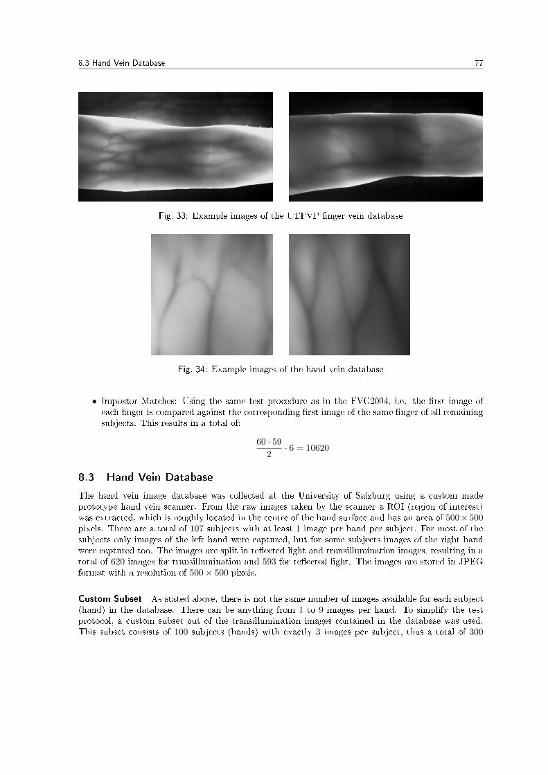
8.3 Hand Vein Database 77
Fig. 33: Example images of the UTFVP �nger vein database
Fig. 34: Example images of the hand vein database
• Impostor Matches: Using the same test procedure as in the FVC2004, i.e. the �rst image ofeach �nger is compared against the corresponding �rst image of the same �nger of all remainingsubjects. This results in a total of:
60 · 59
2· 6 = 10620
8.3 Hand Vein Database
The hand vein image database was collected at the University of Salzburg using a custom madeprototype hand vein scanner. From the raw images taken by the scanner a ROI (region of interest)was extracted, which is roughly located in the centre of the hand surface and has an area of 500× 500pixels. There are a total of 107 subjects with at least 1 image per hand per subject. For most of thesubjects only images of the left hand were captured, but for some subjects images of the right handwere captured too. The images are split in re�ected light and transillumination images, resulting in atotal of 620 images for transillumination and 593 for re�ected light. The images are stored in JPEGformat with a resolution of 500× 500 pixels.
Custom Subset As stated above, there is not the same number of images available for each subject(hand) in the database. There can be anything from 1 to 9 images per hand. To simplify the testprotocol, a custom subset out of the transillumination images contained in the database was used.This subset consists of 100 subjects (hands) with exactly 3 images per subject, thus a total of 300

78 8 Experimental Setup
images. Only transillumination images were used, because the achieved EER is higher compared tousing re�ected light images only and also to using both, transillumination and re�ected light images.
8.3.1 Test Procedure
Again for the hand vein experiments the test protocol of the FVC2004 was adopted.
• Genuine Tests: Each sample image is matched against all remaining samples of the same hand.No symmetric matches are performed. Based on the the custom subset used for evaluation,containing 100 hands with 3 images each, the number of genuine tests is:
nimages · (nimages − 1)
2· nhands =
3 · 22· 100 = 300
• Impostor Tests: Following the FVC2004 test protocol the �rst image of each hand is matchedagainst the �rst image of all remaining hands. As with the genuine tests, no symmetric matchesare performed. Again based on the custom subset, the number of impostor tests is:
nhands · (nhands − 1)
2=
100 · 99
2= 4950
8.4 Simulation Settings
As I was not able to determine the number and parameters of the sensor ageing related pixel defectsdirectly from images captured by the respective sensor due to the lack of usable data, i.e. I had no twodata sets acquired by the same sensor with a timespan of several years in between, the defect growthrate could not be estimated directly. Thus, I used the formula of Chapman et al. [9] to estimate thedefect growth rate for the di�erent sensor types according to the parameters of the particular imagesensor.
8.4.1 Defect Growth Rate
Fingerprint Scanner As I showed in 8.1.2 the Casia data sets of 2013 and 2009 were captured usingdi�erent sensors and thus it was not able to derive the defect growth rate and defect parameters fromthese data sets. So I had to estimate the defect growth rate using the following formula from Chapmanet al. [9], explained in 3.7 :
D = A · SB · ISOC
As I have not got technical information from Digital Persona10 regarding their U.are.U4000B andU.are.U4500 �ngerprint sensors, I did some research on commonly used image sensors for that purpose.The most widely used ones are CMOS sensors with a pixel sizes between 5.0µm and 7.4µm (squarepixels).
I also ordered an U.are.U4000B �ngerprint sensor and disassembled it to have a look at the imagesensor. There was no label on it but I was able to measure the sensor size. In �gure 35 a picture of theimage sensor can be seen. The outside dimensions (dark yellow square) are 10.6× 10.6mm or about410 × 410 pixels in the image. The actual image sensor area (red to yellow rectangle in the left andblue rectangle in the right picture) is about 77× 66 pixels. This means that the sensor's dimensionsare 1.99× 1.71mm which corresponds to a sensor area of 3.404mm2.
The images captured by the U.are.U 4000b and U.are.U 4500 have a resolution of 356×328 pixels,thus, with the measured sensor size of 3.404mm2 the pixel size is: 1.99
356 ×1.71328 = 5.59 × 5.21µm. I
10 http://www.crossmatch.com/UareU4500Reader/
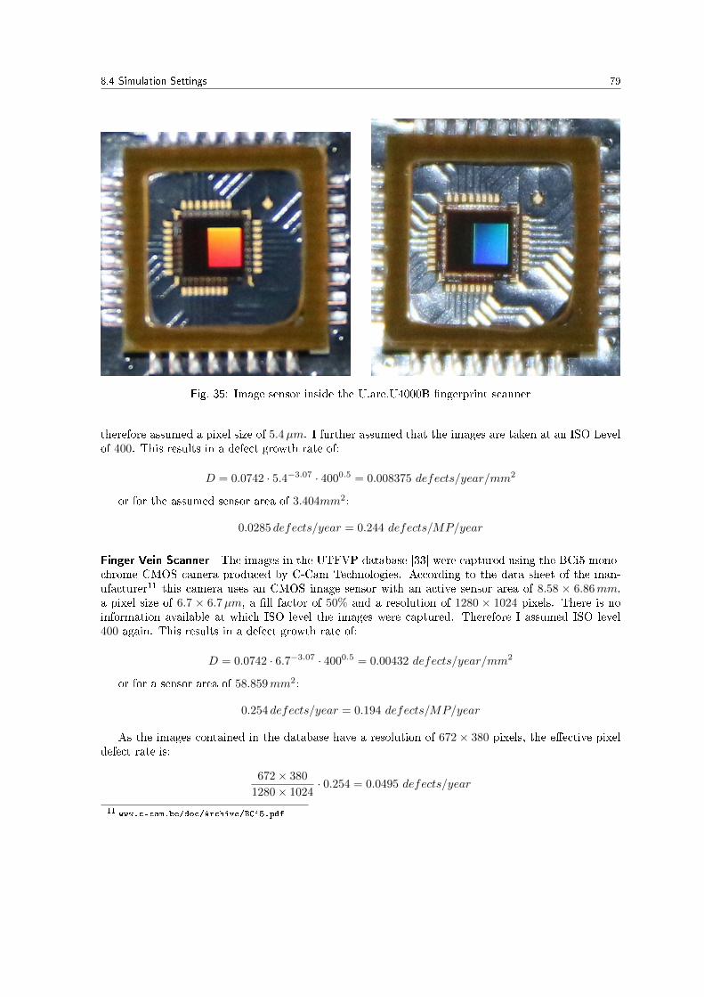
8.4 Simulation Settings 79
Fig. 35: Image sensor inside the U.are.U4000B �ngerprint scanner
therefore assumed a pixel size of 5.4µm. I further assumed that the images are taken at an ISO Levelof 400. This results in a defect growth rate of:
D = 0.0742 · 5.4−3.07 · 4000.5 = 0.008375 defects/year/mm2
or for the assumed sensor area of 3.404mm2:
0.0285 defects/year = 0.244 defects/MP/year
Finger Vein Scanner The images in the UTFVP database [33] were captured using the BCi5 mono-chrome CMOS camera produced by C-Cam Technologies. According to the data sheet of the man-ufacturer11 this camera uses an CMOS image sensor with an active sensor area of 8.58 × 6.86mm,a pixel size of 6.7 × 6.7µm, a �ll factor of 50% and a resolution of 1280 × 1024 pixels. There is noinformation available at which ISO level the images were captured. Therefore I assumed ISO level400 again. This results in a defect growth rate of:
D = 0.0742 · 6.7−3.07 · 4000.5 = 0.00432 defects/year/mm2
or for a sensor area of 58.859mm2:
0.254 defects/year = 0.194 defects/MP/year
As the images contained in the database have a resolution of 672 × 380 pixels, the e�ective pixeldefect rate is:
672× 380
1280× 1024· 0.254 = 0.0495 defects/year
11 www.c-cam.be/doc/Archive/BCi5.pdf

80 8 Experimental Setup
Hand Vein Scanner The custom build hand vein scanner uses a Canon EOS 5D Mark II DLSRcamera as image capturing device. According to Canon this camera uses a CMOS image sensor with asize of 36.0×24.0mm and a resolution of 5616×3744 pixels. Thus it has a pixel size of 6.41×6.41µm.The images were taken at ISO level 800. This results in a defect growth rate of:
D = 0.0742 · 6.41−3.07 · 8000.5 = 0.006997 defects/year/mm2
or for a sensor area of 864mm2:
6.045 defects/year = 0.287 defects/MP/year
According to the literature [6] DSLRs develop between 0.5 and 10 defects per year at ISO Level400 so a value of 6.045 defects per year seems reasonable.
As only a ROI (region of interest) with a size of 500× 500 pixels is used the e�ective pixel defectrate is:
500× 500
5616× 3744· 6.045 = 0.0719 defects/year
8.4.2 Hot and Stuck Pixel Amplitudes
Jessica Fridrich [18] and also others found out that there are stuck low, stuck high and in generalstuck pixels with any value between 0 and 255 (for 8 Bit images). Thus, I assumed that stuck pixelscan appear with any value between 0 and 255, uniformly distributed. According to Chapman et al.[6] but also Albert Theuwissen [3] the additional o�set IOffset of hot pixels or the dark current value,respectively follows an exponential distribution, i.e. hot pixels with a lower amplitude are more likelyto occur.
Estimating the Exponential Distribution To be sure to use an accurate model for the distributionof the hot pixel amplitudes it has to be veri�ed whether they are really exponentially distributed andthen a �tting exponential distribution with the parameter µ has to be determined. First of all, theactual values of the hot pixel amplitudes and the number of hot pixels having these amplitudes haveto be determined. As basis for that �gure 3 (a) in [5], at an exposure time of 1/2 s and for ISO Level400, was used to get the reference data. Chapman uses an Ioffset value, which is according to thepixel model in section 3.4.2, the dark response of a hot pixel, i.e. an additional o�set to the electricalcurrent induced by the incident light, depending on the dark current amplitude, the exposure timeand the ISO level. For each database or set of images I tested, all images were captured using thesame exposure time, ISO level and roughly the same environmental conditions like temperature, i.e.the dark current amplitude should remain constant. So instead of an Ioffset value I used the pixelvalue o�set directly for the simulation of pixel defects. As pixel values between 0 and 255 are used, anIoffset value of 0 simply corresponds to a pixel o�set value of 0 and an Ioffset value of 1 correspondsto a pixel value of 255.
As second source of reference data �gure 6 from [3] was used. There the number of hot spots persensor per day versus the hot spot amplitude in DN (digital numbers) is shown. I assumed that aDN value of 4500 corresponds to a pixel value of 255 and used the corresponding values as pixel o�setvalues then. The values from the two �gures were extracted as follows:
A suitable exponential distribution with its parameter µ was determined using MATLAB's built-ingraphical distribution �t tool dfittool.
For the Chapman data which is given as a histogram, a bin width of 0.2 was used for the inputdata and a corresponding exponential distribution with µ = 0.1438 at a standard error of 0.00045437was found.

8.4 Simulation Settings 81
Fig. 36: Hot pixel amplitudes, top: Chapman et al. [5], bottom: Theuwissen, Albert [3]

82 8 Experimental Setup
Ioffset defect count (%)
0.1 87.3
0.3 8.3
0.5 1.9
0.7 1.2
0.9 0.2
1 1.1
Hot Spot Amplitude (DN) Number of hot spots
0 0.6856
250 0.1208
500 0.06122
750 0.03475
1000 0.02569
1250 0.01762
1500 0.01254
1750 0.00893
2000 0.00712
2250 0.005264
2500 0.003892
2750 0.003346
3000 0.002668
3250 0.001973
3500 0.00119
Tab. 5: Defect counts of hot pixels with a certain amplitude, left: Chapman data, right: Theuwissendata
For the Theuwissen data at �rst the DN values were normalised by dividing each value by 4500 toget values in the interval of [0, 1]. But at �rst no suitable exponential distribution was found, so the�rst value which corresponds to DN = 0 and actually means that it is no hot pixel at all (having a hotspot amplitude of 0) was omitted. Still no exponential distribution could be found, so I interpretedthe diagram as a histogram with a bin width of 250
4500 = 0.05556 and then best �t was obtained usingµ = 0.16839 with a standard error of 0.000961.
8.4.3 Simulation Parameters
The resulting defect rates according to the estimations are rather low, ranging from 0.028 to 0.072defects per year, i.e. less than 1 defect per year. Statistically, even in 30 years there would only be1 or 2 defective pixels visible in the �nger or hand images. I started the simulations using a defectrate of 1 defect per year, with a simulation timespan of 30 years to get realistic results (no one woulduse a camera or biometric sensor for more than 30 years). The defect rate was doubled each time, i.e.2 defects per year, 4 defects per year and so on, and the simulation was run again until there werenoticeable e�ects on the recognition accuracy. As the defects were only barely noticeable below 1000defects contained in a single image, I modi�ed the simulation parameters and ran the simulation witha defect rate of 1000 defects per year for a time span of 10 years, which results in a total of 10000hot or stuck pixel defects or 20000 hot and stuck pixels combined, respectively. Note that using both,stuck and hot pixel defects, the defect rate is twice as high as using a single defect type. The resultsonly show the total number of defects, i.e. the combined defect rate is given.
The �ngerprint images of the FVC2004 DB1 and DB2 have di�erent resolutions. Also the �ngervein and hand vein image resolutions are di�erent from that of the �ngerprint images. If a defectrate of 1000 defects per year is used, this results in a higher defect density for images with a smallerresolution and a lower defect density for images with a higher resolution, respectively. A higher defectdensity has a higher impact on the recognition accuracy. To be able to compare the results among eachother, a defect rate per year per MP was used. The simulations were done for �nger vein images �rstusing a defect rate of 1000 defects per year. These images have a resolution of 672× 380 = 0.255MP ,

8.4 Simulation Settings 83
thus for the other simulations a defect rate of 4000 defects/MP/year was used.The stuck pixel amplitudes were drawn uniformly out of the interval [0, 255] and the hot pixel
amplitudes were drawn according to an exponential distribution with µ = 0.15.All simulations were run using only stuck pixel defects, only hot pixel defects and then both, stuck
and hot pixel defects, respectively.During the tests two sets of images were used: the gallery database, which contains the unaged
images and the probe database, which contains the aged images. In other words the template imageswere not aged, only the probe images were. This means that in each pair of matched images only oneis aged, the other one is the original image from the data set. In addition for some of the experiments,also the template images were aged using the same defective pixels as the probe images to be ableto examine the e�ects. In the case of gallery images aged, this is denoted with TA (templates aged)in the diagrams and in the text. An application scenario where also the gallery images are a�ectedby sensor ageing is the use of an �old� biometric sensor, i.e. a sensor that was in use for at least afew years, for establishing a biometric database. In this case the probe images will contain ageingrelated pixel defects which will become more severe with increasing sensor age. In addition also thegallery images will contain some ageing related pixel defects, depending on the point in time when thedatabase was established. For a thorough investigation of course all combinations of di�erent progressin the ageing process should be tested. E.g. the database could have been established in year 1 andthe probe images could be captured in year 12, or the database could be established in year 10 andthe probe images also captured in year 10. Due to time restraints this would have been beyond thescope of this thesis so only the combinations where the gallery and probe images are captured at thesame point in time, i.e. show the same ageing related pixel defects, were tested.

84 8 Experimental Setup

85
9 Results
This section presents the experimental results from running the ageing simulation for the di�erentbiometric traits, i.e. �ngerprint, �nger vein and hand vein, and also the di�erent matchers used foreach trait aimed to investigate the impact of sensor ageing related pixel defects on the recognitionperformance of each of the feature extraction and matching schemes used for the di�erent biometrictraits. More information on the experimental settings, especially the simulation parameters, the testdata sets and the test protocol, can be found in section 8. The following subsection introduces someabbreviations for the evaluated feature extraction and matching schemes. After that each subsectiondeals with a speci�c biometric trait, beginning with �nger veins, followed by hand veins and �nally�ngerprints. In each of these three subsections �rst of all the tested schemes are listed and speci�csettings or tests are described, if any. In addition some sample aged images for each trait are given.Afterwards the experimental results are provided in form of a table, stating the baseline EER and theEERs for the aged images, and diagrams showing the EER at di�erent numbers of defective pixelsfor each of the evaluated approaches. This is followed by a discussion of the results. Not only theresults of each individual approach are discussed but they are also compared to the other approachesthat were tested. In addition I also try to give some explanations why some approaches are in�uencedwhereas other are not and how to reduce the impact in general.
9.1 Abbreviations
The following list shows the abbreviations for the di�erent feature extraction and matching schemesused in the diagrams and the text.
• MC: Maximum Curvature, described in section 7.3.1. Feature extraction method which wasused for �nger vein and also for hand vein evaluations.
• SIFT: SIFT based feature extraction method, also used for �nger vein and hand vein evaluations,described in section 7.3.7.
• WLD: Huang Wide Line Detector, described in section 7.3.3. This is the second feature extrac-tion method which is used for �nger vein and hand vein experiments.
• RLT: Repeated Line Tracking, feature extraction method used only for �nger vein experimentsdue to its high runtime and inferior results on hand vein images. Described in section 7.3.2.
• LBP: Local Binary Patterns, another feature extraction method which is described in section7.3.5. This was only used for �nger vein images due to its inferior results on hand vein imagescompared to MC and SIFT.
• AB: Adaptive Binarisation or Template Matching as the last feature extraction method whichwas used for �nger vein and hand vein experiments. Details are described in section 7.3.6.
• NBIS: Means the mindtct minutiae extractor and bozorth3 matcher from the NIST BiometricImage Software package. Details can be found in section 6.4.3. NBIS was used for �ngerprintimages only.
• VF: VeriFinger matcher from Neurotechnology. This is a commercial package of a minutiaebased feature extractor and matcher for �ngerprint images. Details can be found in section6.4.3. A trial version was used during the �ngerprint evaluations.
• POC: Phase Only Correlation, a correlation based matcher for �ngerprint images. A customimplementation was used, details are described in section 6.4.1.

86 9 Results
• FC: Finger Code is a ridge feature based matcher for �ngerprint images. Details of the customimplementation which was used during the evaluations can be found in section 6.4.2.
9.2 Finger Vein Results
In this subsection the results of the �nger vein experiments are lined out. MC, RLT, WLD, LBP,AB and the SIFT based approach were tested. The simulations were run for hot pixels only, stuckpixels only and combined hot and stuck pixels. All simulations were run 5 times, i.e. 5 test sets withaged images are created. All the feature extraction and matching schemes are evaluated for each testset. The sensor defects are randomly distributed over the image and also the amplitudes or hot pixelo�sets, respectively, are random values. Due to the random nature of the defect locations and values,some defective pixels may have a larger in�uence on the recognition accuracy than others, e.g. if thereare several hot pixels inside a vein. Running the simulations 5 times should mitigate these e�ects but,as it can be seen on the results, not completely as there are still some statistical �uctuations. Themean of the EER is used as �nal result.
In addition, all evaluations were done using a denoising �lter (median �lter followed by an adaptiveWiener �lter) during the preprocessing step, which reduces the sensor ageing related impact to a greatamount even for those schemes which are heavily in�uenced. One drawback is that the baseline EERrises, i.e. the recognition accuracy drops if denoising is used. Also note that the results for LBP arethe same with and without denoising as LBP uses denoising by default.
9.2.1 Sample Aged Images and Corresponding Feature Extraction
In �gure 37 some sample �nger vein images with no defects, 1000 and 10000 pixel defects and thecorresponding region of the feature extraction image for MC, RLT and WLD are shown. One canclearly see that for MC due to the pixel defects the lines get broken and an additional line appears at10000 defects which is clearly not a vein. The vein lines do not get broken in the case of RLT but theyappear wider with some additional noise at the vein boundaries. WLD does not show much usefulinformation any more at 10000 defects due to the noise caused by the defective pixels which appearsas small circles inside the image.
9.2.2 Simulation Results
Table 6 shows the baseline EER for all the tested approaches with and without denoising. As statedabove, in the case of MC, RLT and SIFT the baseline EER rises when denoising is used. In additionalso the EER for 10000 defects present in the images (5000 hot and 5000 stuck pixels) are shown withand without denoising. Furthermore the percental rise of the EER compared to the correspondingbaseline EER is given right next to each absolute EER value. By comparing the baseline EER valuesof the di�erent approaches, it can be clearly seen that MC performs best with an EER of 0.006. Thesecond best performing approach is RLT closely followed by SIFT, both achieving an EER of 0.02which is more than 3 times higher than MC. On the fourth place is WLD with an EER of 0.031followed by AB with 0.036. The worst performing approach is the LBP based one with an EER of0.063, which is more than 10 times higher than the best performing approach, MC.
Figure 38 shows that not only SIFT and MC but also the simple AB scheme (presumably becauseit additionally relies on the �nger outline and not solely on the vein structure) is hardly in�uencedat all by hot pixel defects, even if there are 10000 defects inside the image. The EER of MC risesto 0.0074 at 10000 defects but it is still the best performing approach. The EER of RLT doubles at10000 defects but stays still below 0.045 so it is on the fourth place while SIFT gets on the secondone with an EER of 0.024. The EER of AB rises to 0.043, which is a bit better than RLT and on thethird place regarding the matching performance. WLD, as it is quite a simple thresholding method, is
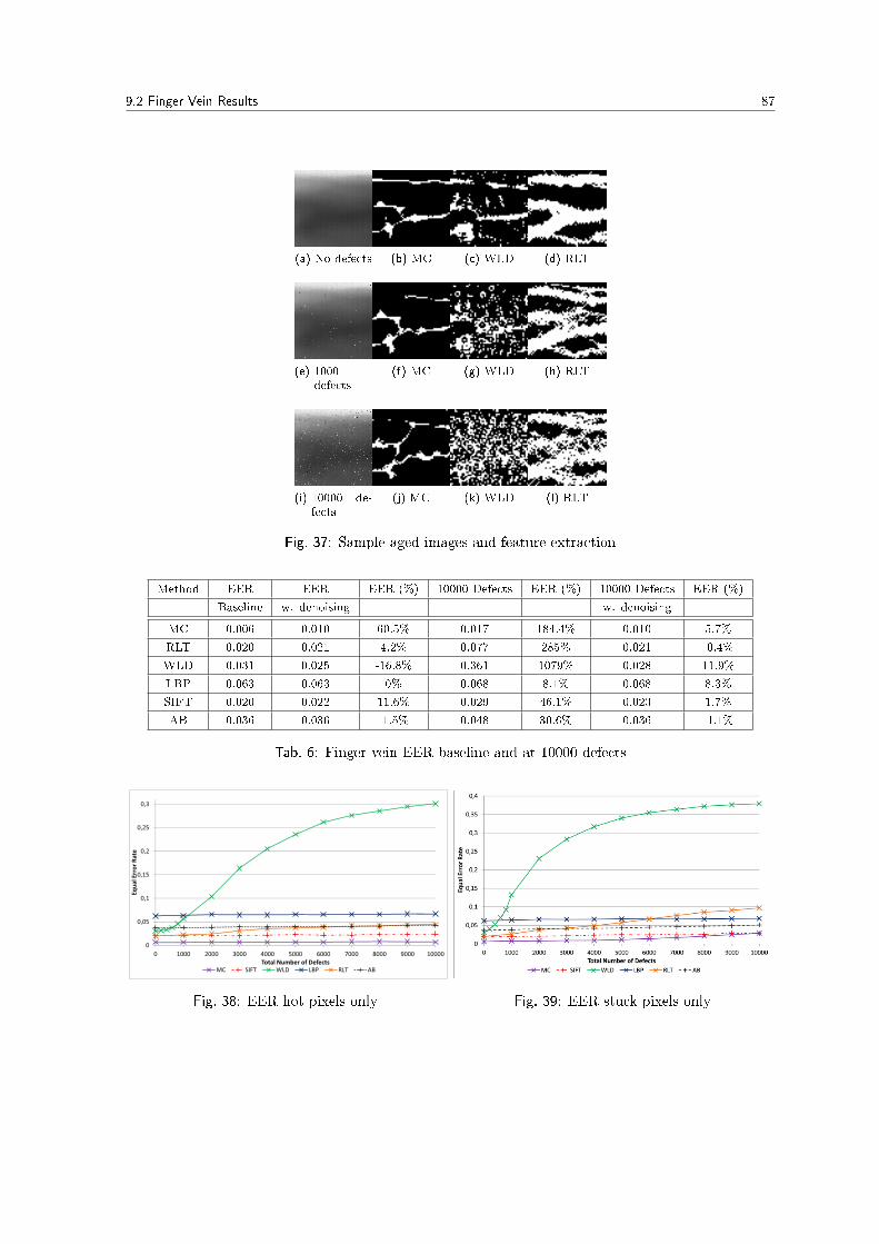
9.2 Finger Vein Results 87
(a) No defects (b) MC (c) WLD (d) RLT
(e) 1000defects
(f) MC (g) WLD (h) RLT
(i) 10000 de-fects
(j) MC (k) WLD (l) RLT
Fig. 37: Sample aged images and feature extraction
Method EER EER EER (%) 10000 Defects EER (%) 10000 Defects EER (%)
Baseline w. denoising w. denoising
MC 0.006 0.010 60.5% 0.017 184.4% 0.010 5.7%
RLT 0.020 0.021 4.2% 0.077 285% 0.021 -0.4%
WLD 0.031 0.025 -16.8% 0.361 1079% 0.028 11.9%
LBP 0.063 0.063 0% 0.068 8.1% 0.068 8.3%
SIFT 0.020 0.022 11.6% 0.029 46.1% 0.023 1.7%
AB 0.036 0.036 -1.5% 0.048 30.6% 0.036 -1.1%
Tab. 6: Finger-vein EER baseline and at 10000 defects
�
����
���
����
���
����
���
� ���� ���� ���� ���� ���� ���� ��� ��� ���� �����
��������������
������������ ��� ����
� ���� ��� ��� ��� ��
Fig. 38: EER hot pixels only Fig. 39: EER stuck pixels only

88 9 Results
�
����
���
����
���
����
���
����
���
� ���� ���� ���� ��� ����� ����� ����� ����� ���� �����
��������������
������������ ��� ����
� � �� ��� ��� ��� ��
Fig. 40: EER hot and stuck pixels
in�uenced dramatically. At 10000 defects the EER is 0.301 and thus ten times higher than its baselineEER. Hence it is the worst performing approach. The performance of LBP is hardly in�uenced at allby the noise introduced due to sensor ageing, even in the case of 10000 defects, its EER is 0.067 whichcorresponds to an increase of 6.5%. LBP uses denoising by default but it is still no better than the�fth place regarding the performance ranking.
In �gure 39 it can be seen that the in�uence of stuck pixels is more severe than of hot pixels.The average amplitude or hot pixel o�set, respectively, is quite low thus the original grey value isonly slightly changed. Stuck pixels always have the same �xed value, independent of the original greyvalue, so they are actually more likely to �break� the vein lines inside the image.
SIFT is again quite stable with an EER of 0.028 at 10000 hot pixel defects, which is now placed�rst in the performance ranking. MC is a�ected more by stuck than by hot pixels and at 10000 defectsthe performance of MC gets slightly worse than the SIFT one with an EER of 0.029, which meansit is the second best approach. Also the performance of AB is in�uenced more by stuck pixels thanby hot ones as the EER rises to 0.051 at 10000 stuck defects in comparison to 0.043 for hot ones butit is again on the third place. RLT is in�uenced more than MC and AB as its EER rises to 0.097 incomparison 0.045 at 10000 hot pixel defects and thus it is on the fourth place. In accordance with MC,AB, RLT and SIFT, WLD is also in�uenced more by the stuck pixel defects. The EER of WLD risesto 0.379 at 10000 stuck pixel defects, which is again the last place regarding matching performance.Only for LBP the impact of stuck pixels is not signi�cantly higher than for hot pixels due to denoising.Its EER for 10000 stuck pixels is 0.069 and it is on place four in the ranking this time.
If both, hot and stuck pixel defects, are present in the images, similar results as with the singledefect types can be seen. WLD is in�uenced most and again the worst performing approach, whereasthe performance of SIFT is quite stable, even if 20000 defects in total (10000 hot and 10000 stuckpixels) are present, i.e. the EER rises to 0.032. SIFT is the best performing approach at 20000 defects.The performance of MC gets worse than SIFT at 14000 defects (MC: 0.03 and SIFT: 0.027) and at20000 defects it is the second best performing approach, only slightly ahead of AB which is on thethird place. RLT is a�ected more than by hot pixels only but not as much as by stuck pixel defectsonly. At 20000 defects it performs worse than LBP and is the second worst performing approach. ItsEER for a total of 10000 defects is 0.077 and at 20000 defects it is 0.111. The in�uence on LBP andAB is again negligible. The EER of LBP at 20000 defects is 0.07, thus it is on the fourth place in theperformance ranking. AB achieves an EER of 0.054 at 20000 defects, which means it is the third bestperforming approach.
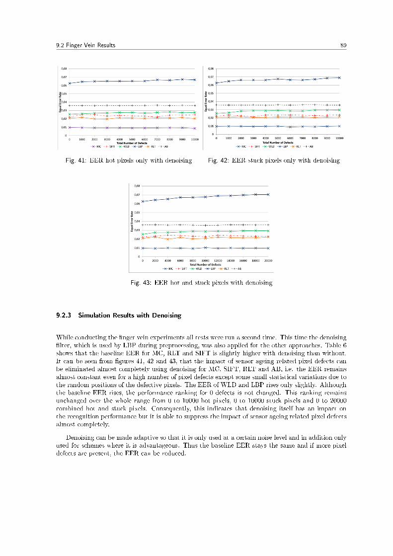
9.2 Finger Vein Results 89
Fig. 41: EER hot pixels only with denoising Fig. 42: EER stuck pixels only with denoising
Fig. 43: EER hot and stuck pixels with denoising
9.2.3 Simulation Results with Denoising
While conducting the �nger vein experiments all tests were run a second time. This time the denoising�lter, which is used by LBP during preprocessing, was also applied for the other approaches. Table 6shows that the baseline EER for MC, RLT and SIFT is slightly higher with denoising than without.It can be seen from �gures 41, 42 and 43, that the impact of sensor ageing related pixel defects canbe eliminated almost completely using denoising for MC, SIFT, RLT and AB, i.e. the EER remainsalmost constant even for a high number of pixel defects except some small statistical variations due tothe random positions of the defective pixels. The EER of WLD and LBP rises only slightly. Althoughthe baseline EER rises, the performance ranking for 0 defects is not changed. This ranking remainsunchanged over the whole range from 0 to 10000 hot pixels, 0 to 10000 stuck pixels and 0 to 20000combined hot and stuck pixels. Consequently, this indicates that denoising itself has an impact onthe recognition performance but it is able to suppress the impact of sensor ageing related pixel defectsalmost completely.
Denoising can be made adaptive so that it is only used at a certain noise level and in addition onlyused for schemes where it is advantageous. Thus the baseline EER stays the same and if more pixeldefects are present, the EER can be reduced.

90 9 Results
9.2.4 Interpretation of the Results
MC MC tries to emphasise the centre lines of the veins, thus it generates binary images where thewidth of the vein lines should be 1 pixel. In addition MC uses a �ltering operation to connect brokenvein lines. Therefore it is quite insensitive to sensor ageing related pixel defects, which are pointlike, single pixel defects. On the one hand the �ltering operation reconnects vein lines that might getbroken due to defective pixels, on the other hand if a vein might get thicker due to stuck low pixels,this e�ect is mitigated by emphasising only the centre lines of the veins. If the number of defectivepixels rises, vein lines might get broken because the �ltering operation cannot connect them any more.This is why the performance of MC drops at some point. As it can be seen from the �gures, MC ishardly in�uenced at all if only hot pixels are present. A hot pixel simply adds an o�set to a pixelvalue, thus the pixel appears brighter. As the veins appear as dark lines in the image, bright pixelswill only break the vein lines, which is corrected by the �ltering operation of MC. Stuck pixels have amore severe in�uence on MC because they might be stuck at any pixel value between 0 and 255, i.e.also dark values. Thus, a stuck pixel can �extend� a vein line at least by one pixel and if there areseveral stuck pixels in the same image area, the �ltering operation might connect the stuck pixel and�generate� a false vein line.
Using a denoising �lter reduces the baseline performance of MC because it gets more di�cult toaccurately extract the centre lines of the veins as due to denoising the vein boundaries get less sharpthan without it. But this simple denoising �lter is able to mitigate the e�ect of hot and also stuckpixels on MC almost completely as the EER remains nearly constant not only up to 10000 hot or stuckpixels, respectively, but also up to 20000 pixel defects in total (10000 hot and 10000 stuck pixels).
SIFT SIFT tries to extract keypoints only out of �relevant� areas inside the image, i.e. it is alsoable to handle noise contained in the image. The keypoint extraction algorithm tries to extract thekeypoints according to image information, like edges, high frequency content, etc. It is able to handlea certain amount of point like noise well. Like MC also SIFT is in�uenced more by stuck than byhot pixels. But the in�uence for a realistic number of pixel defects occurring in practical applications,which are much less than 1000 defects per sensor, is negligible. Even for 20000 defects in total its EERonly rises from 0.02 to 0.032 which is a rise of 60%. Although SIFT is only the second best performingscheme, it is less in�uenced by pixel defects than the best performing approach, MC, which can beseen by comparing the percental rise of the EER. The in�uence of hot pixels might be lower than forstuck pixels because a hot pixel only adds an o�set to a pixel value, i.e. the region containing thepixel stays smooth to a certain degree, whereas a stuck pixel has an arbitrary but �xed value, whichmight be totally di�erent compared to its surrounding pixels.
Using denoising the baseline EER of SIFT gets higher but as with MC it remains almost constantup to 20000 pixel defects except some statistical variations. This means that also the SIFT basedapproach has no di�culties to deal with sensor ageing related pixel defects in practice.
RLT As it can be seen in �gure 37, the vein lines do not get broken if Repeated Line Trackingis used as feature extraction method. But they appear brighter and have some additional noise onthe vein boundaries. This is because of the way RLT works. It tries to extract the vein lines byrepeatedly tracking dark lines inside the image. Dark means the pixel's value is darker compared toits neighbours. If there are several hot pixels inside the image, a pixel which actually does not belongto a vein line might appear dark enough for RLT to count it as vein. RLT records the number oftimes each pixel is detected as belonging to a vein and applies a simple thresholding to these valuesafterwards to get the binary output image. This means that it is not independent of the vein widthand especially if there are some hot pixels present along the boundaries of the veins, additional pixels,that are actually outside the vein but appear not as bright as the pixels further outside, may be

9.2 Finger Vein Results 91
detected as still belonging to the vein because the pixels further outside appear brighter due to thehot pixels. The EER of RLT rises from its baseline EER of 0.02 to 0.043 for 10000 hot pixels. Againthe in�uence of stuck pixels is more severe as the EER rises to 0.051 for 10000 stuck pixels. The sameas in the case of MC holds, i.e. a stuck low pixel is directly counted as vein line, thus especially stucklow pixels have a high in�uence on RLT. But also stuck high pixels lead to a drop in the recognitionaccuracy because they have the same e�ect as hot pixels and might lead to an increase in the widthof the extracted vein lines with some additional noise on the vein boundaries.
The simple denoising �lter is again able to mitigate the e�ects of sensor ageing almost completely.The EER of RLT remains quite constant even up to 10000 hot, 10000 stuck or 20000 combined hotand stuck pixel defects. Its baseline EER rises from 0.02 to 0.021 which is only a rise of 4%. ItsEER for 10000 hot pixels is 0.0205, for 10000 stuck pixels it is 0.0211 and for 20000 pixel defects itis 0.0228 which results in a rise of 9% in the worst case. Thus also RLT can be made robust againstsensor ageing related pixel defects using a simple denoising �lter with only a small drop in the baselinerecognition performance.
WLD WLD basically uses a simple local adaptive thresholding technique to extract the vein linesfrom the background. It compares the centre pixel to its neighbouring pixels inside a circular neigh-bourhood. If the centre pixel is in�uenced by a hot or a stuck pixel defect, this has a severe in�uenceon the binary output image. As it can be seen in �gure 37, the defective pixels are causing noise thatappears as small circles in the binary output images. This is the main reason why WLD is heavilyin�uenced by both, hot and stuck pixel defects. Again the in�uence of stuck pixels is higher than forhot pixels, that is mainly due to the rather low hot pixel o�sets, which do not in�uence the adaptivethresholding so much. But it is the approach, which is in�uenced most by sensor ageing related pixeldefects as its EER is more than 10 times higher than the baseline EER for 10000 hot and also for10000 stuck pixel defects. This suggests that WLD is also sensitive to other types of image distortions,which may occur during practical use of �nger vein recognition systems.
Again denoising is able to reduce the impact of the sensor ageing related pixel defects to a minimum.For WLD the baseline EER improves when using denoising as it is only 0.025 compared to 0.031without denoising. The EER for 10000 hot pixels is 0.028, for 10000 stuck pixels it is 0.03 and for20000 combined stuck and hot pixels it is 0.029, which is even lower than for 10000 stuck and onlyslightly higher than for 10000 hot pixel defects. In either case the rise of the EER is less than 17%(8.4% for hot, 16.3% for stuck and 14.8% for hot and stuck pixels combined).
LBP LBP compares the value of a centre pixel to its neighbouring pixels where the output valuedepends on the binary pattern of the neighbouring pixels inside a 3× 3 neighbourhood. Here a multi-scale LBP operator was used, which repeats this comparison for several resized versions of the imagetrying to make the output more robust against noise and small perturbations. As stated above, LBPuses denoising during preprocessing by default. Thus the impact of hot and stuck pixels is relativelylow compared to LBP without denoising which was also tested. This is quite obvious because alreadya single pixel, which changes its value inside the neighbourhood, changes the output value completely.Also the baseline EER of LBP would much higher without denoising and LBP was only evaluated withdenoising. Using denoising the image is smoothed and the spiky noise is suppressed. Thus the impactof the pixel defects is manageable but LBP has the worst performance of all the tested approaches. Itsbaseline EER is 0.063, which is more than 6 times higher than the baseline EER of the best performingapproach, MC. LBP is in�uenced slightly more by stuck pixels than by hot pixels only as its EERfor 10000 stuck pixels rises to 0.069 compared to 0.067 for 10000 hot pixels only. Its EER for 20000combined stuck and hot pixels rises to 0.07 which is a rise of 12% and thus the second highest dropin recognition performance after WLD (with denoising).

92 9 Results
AB The adaptive binarisation or template matching approach is a generic adaptive thresholdingtechnique, which is even simpler than WLD but it is much less in�uenced by sensor ageing thanWLD. If the binary output images of AB are inspected, the �nger boundaries can be clearly seen,whereas small veins do not appear in the output images. Single pixel defects mostly in�uence smallstructures inside the image like the small and thin veins but bigger structures like the �nger boundariesare not in�uenced so much. Thus my assumption is that AB relies on the �nger outline to a greatextent and on thicker vein lines, which reduces its baseline EER compared to the other approaches, butmakes it more robust against single pixel defects. For 10000 hot pixel defects and also for 10000 stuckpixel defects it performs better than RLT, LBP and WLD. For 20000 combined defects it performsnearly as good as MC. Its EER rises only slightly even without denoising. Its baseline EER is 0.036and its EER for 10000 hot pixel defects is 0.043, for 10000 stuck pixel defects it is 0.051 and for20000 combined defects it is 0.055. This means a rise of 17.5%, 40% and 50%, respectively. The factthat the rise in the EER is higher compared to hand veins shows that it does not solely rely on the�nger outline as there is no �nger or hand outline visible in the hand vein ROI pictures used duringevaluation.
Using denoising the baseline EER of AB remains nearly the same (it actually slightly drops) andin addition it remains constant except some very small statistical variations for hot, stuck and alsocombined hot and stuck pixels. Thus in the case of AB denoising is able to mitigate the e�ect ofsensor ageing on the recognition performance completely.
9.2.5 Finger Vein Conclusion
According to the estimation done with the empiric formula in section 8.4.1 a defect rate of 0.05defects/year would occur for the type of sensor used in the �nger vein scanner. This defect rate isreally low and would statistically lead to 1.5 defective pixels over a reasonable long sensor lifetime of30 years. I showed that the impact of less than 1000 pixel defects per image is negligible for all of thetested approaches. Thus, the impact of sensor ageing and its related pixel defects for a reasonable,i.e. realistic number of defective pixels that will occur in practice, is negligible.
Even for the unrealistic number of 10000 (which is about 10000 times the number of defects thewhole sensor would develop in 20 years) pixel defects, SIFT is hardly in�uenced at all because itskey point extraction algorithm is robust against that type of noise. The in�uence on MC is quitelow because it emphasises only the centre lines of the veins and uses a �ltering operation, whichreconnects broken vein lines and �lters out some noise at the vein boundaries. RLT, LBP and thesimple AB scheme are also relatively robust against the defects up to a rather high number of defectivepixels. Only the performance of WLD drops signi�cantly. Using a simple denoising �lter the baselineperformance slightly drops, i.e. the EER rises, but the in�uence of sensor ageing can be substantiallyreduced even for WLD. As mentioned above denoising can be made adaptive, so that it is only usedif the performance drop is higher than it would be due to denoising.
In conclusion sensor ageing is not an issue for practical applications of �nger vein recognition.
9.3 Hand Vein Results
This subsection presents the results regarding simulations and experiments done using the hand veindata. For evaluating the impact of sensor ageing on hand vein based biometric recognition systems,some of the feature extraction and matching schemes from �nger vein recognition have been used.Speci�cally MC, SIFT, WLD and AB were used during the experiments. Again all simulations wererun 5 times for hot pixels only, stuck pixels only and combined hot and stuck pixels using a defectrate of 4000 defects/MP/year for 10 years with a time step of 1 year.
As the rotation correction done for �nger vein images is based on the �nger outline and cannotbe done for the hand vein images (only the ROI images are used which do not contain the outline of
9.3 Hand Vein Results 93
Method Baseline EER 10000 Hot EER (%) 10000 Stuck EER (%) 10000 Hot+Stuck EER (%)
MC 0.013 0.016 19.2% 0.017 25.8% 0.016 20.6%
MC TA 0.013 0.016 20.6% 0.022 61.4% 0.019 40%
SIFT 0.02 0.027 30.7% 0.03 47.6% 0.029 43.9%
SIFT TA 0.02 0.024 16.9% 0.023 14.1% 0.021 2.6%
WLD 0.073 0.112 52.9% 0.177 142.1% 0.161 120.2%
AB 0.157 0.163 3.9% 0.185 18% 0.174 11.2%
Tab. 7: Hand-vein EER baseline, 10000 hot, stuck and combined hot and stuck pixels
the hand or �ngers), the rotation correction has to be done during the matching process. Thereforethe Miura matcher was extended to repeat the matching process several times using rotated versionsof the test image. Of course also the vertical and horizontal shift correction in the same way as with�nger vein images is still performed (matching with slightly shifted versions of the image and usingthe highest matching score as result). I found out that the best compromise between runtime andmatching performance is to use steps of 0.5° in a range of ±5°. A more sophisticated way of doingrotation and translation correction would be an alignment based on the vein crossings like it is done in[1]. On the one hand such an alignment is more complex and prone to errors because the vein patternshave to be extracted at �rst and then the vein �minutiae� have to be found and matched. On theother hand it will speed up the matching process and may improve the matching results. Note thatthis is not necessary for SIFT as it is rotation invariant. In addition, as the structures of hand veinsare di�erent compared, to �nger veins the parameters of the preprocessing �lters were adjusted. Inparticular the parameters of the Circular Gabor Filter and the High Frequency Emphasis Filter wereslightly modi�ed. Furthermore, the feature extraction parameters for WLD and AB were adjusted toaccount for the wider veins compared to �nger veins.
9.3.1 Sample Aged Images
Figure 44 shows 2 hand vein images and the corresponding aged images containing 10000 defectivepixels (5000 hot and 5000 stuck pixels).
9.3.2 Simulation Results
In table 7 the baseline EER for all the tested hand vein approaches and also the EER at 10000 hotpixels, at 10000 stuck pixels and at 10000 combined hot and stuck pixels is listed. Again also thepercental rise of the EER compared to the corresponding baseline EER is given right next to eachabsolute EER value. By comparing the baseline EER values of the four tested approaches, it clearlyshows that MC is the best approach again with an EER of 0.013. The performance of MC is lower forhand veins than for �nger veins (baseline EER is more than doubled). The second best performingapproach is SIFT, achieving an EER of 0.02 which is nearly the same as with �nger veins and thistime only 1.5 times higher than MC. On the third place is WLD with an EER of 0.073 which is muchhigher than for �nger veins. The worst performing method is the simple thresholding scheme, ABwith an EER of 0.157, which is also much higher than for �nger veins. The other methods, i.e. RLTand LBP, were not tested because their performance was inferior compared to the the four testedschemes.
Figure 45 shows the performance in terms of the EER if only hot pixels are present in the probeimages. First of all, it can be seen that the ranking of the 4 tested schemes does not change, evenup to 10000 hot pixels. MC is the best, followed by SIFT, then WLD and the worst performingscheme is AB. It also shows that in the context of hand vein recognition MC is hardly in�uenced
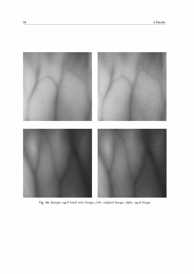
94 9 Results
Fig. 44: Sample aged hand vein images, left: original image, right: aged image

9.3 Hand Vein Results 95
Fig. 45: EER hot pixels only
�
����
����
����
����
���
����
����
����
����
���
� ���� ���� ���� ���� ��� ���� ��� ���� ���� �����
��������������
������������ ��� ����
� �� �� ��� ��
Fig. 46: EER stuck pixels only
at all by hot pixels, it EER at 10000 hot pixel defects is 0.016 which means a rise of 17.6%. EvenSIFT is in�uenced more than MC for hand vein recognition as its EER at 10000 hot pixel defects is0.027, which corresponds to a rise of 30.7% compared to its baseline EER. The simple AB scheme,although the worst performing approach, is in�uenced least. Its EER at 10000 hot pixels is 0.163,which corresponds to a rise of only 3.9%. Like for �nger veins also for hand veins, WLD is in�uencedmost by hot pixel defects and shows an EER of 0.11 or a rise in EER of 50.2%, respectively, at 10000hot pixel defects. Due to the larger width of the hand veins compared to �nger veins this rise is lesssevere than for �nger veins.
The next �gure, �gure 46, shows the EER behaviour if the images are aged with stuck pixels only.Again the ranking of the 4 approaches does not change up to 10000 stuck pixels. The best approachis MC, followed by SIFT, then WLD and AB as last one. Similar to the situation with �nger veinrecognition also here the in�uence of stuck pixels is higher than of hot ones which is most visible forWLD and AB. The EER of WLD at 10000 stuck pixels has a value of 0.176 which is a rise of 140%compared to the baseline EER. This is nearly 3 times higher than for hot pixels. The EER of ABincreases by 18% to 0.185 which is more than 4 times the increase for hot pixels. MC settles at anEER of 0.0168 for 10000 stuck pixels, which is equal to a rise of 26% and thus more than for hotpixels.
The following are the results for both, hot and stuck pixels combined, which can be seen in �gure47. Once again the ranking of all the tested schemes does not change during the whole range of 0 to20000 defects in total, except that WLD gets worse than AB at 20000 defects. Here it is the samesituation as with �nger veins again. The impact of combined hot and stuck pixels is higher than forhot pixels only but it is lower than for stuck pixels only, which is another hint that stuck pixels have ahigher in�uence in general. Please note that the x-coordinate ranges up to 20000 defects in total butto make a more meaningful comparison possible, I mainly state the values at 10000 defects in total.MC achieves an EER of 0.15 at 10000 defects in total, which is even better than for hot pixel defectsonly. SIFT settles at an EER of 0.029, which is higher than for hot but lower than for stuck pixelsonly. WLD has an EER of 0.162, which is a bit lower than for stuck pixels only and higher than forhot pixels only. AB is in�uenced less than for stuck pixels only and hits an EER of 0.174 for 10000defects in total, again following the trend that the EER is higher than for hot pixels only and lowerthan for stuck pixels only.
9.3.3 Interpretation of the Results
MC First of all the performance of MC in the context of hand vein recognition is lower comparedto �nger vein recognition. This might be because there are less veins visible in the images compared

96 9 Results
�
����
����
����
����
���
����
����
����
����
���
� ���� ���� ���� ���� ����� ����� ����� ����� ����� �����
��������������
������������ ��� ����
�� � ��� ��
Fig. 47: EER hot and stuck pixels
to �nger vein images, thus the extracted vein patterns exhibit fewer distinctions. As it can be seenin the �gures 45, 46 and 47, the in�uence of the sensor ageing related pixel defects is lower comparedto �nger veins for all types of defects, i.e. hot pixels only, stuck pixels only and also hot and stuckpixels combined. Figure 44 shows some samples of aged hand vein images. It can be clearly seen thatthe vein structures are bigger compared to the relatively thin �nger veins, i.e. hand veins are widerthan �nger veins. Thus the single pixel defects have less in�uence on the visible vein pattern insidethe image, i.e. they cannot break the vein lines so easily. As mentioned before, MC only extractsthe centre lines of the veins and uses a �ltering operation to reconnect broken vein lines and to �lterout noise at the vein boundaries. Due to that, the in�uence of single pixel defects on the featureextraction is rather low, even lower as with �nger veins, as long as the number of defects stays withina reasonable range. Although the in�uence on MC for hand veins is lower than for �nger veins, stuckpixels have a higher in�uence than hot and stuck pixels combined, which have a higher in�uence thanhot pixels only like it is the case for �nger veins.
SIFT The baseline performance of SIFT is nearly the same as with �nger veins. Figures 45, 46and 47 show that there are some variations in the EER values with an increasing number of sensordefects but there is still a clear trend visible. These variations are due to score calculation methodused for SIFT, which is �count only� instead of �ratio score calculation� as it showed superior results.Count only means that the matching score is simply the total number of keypoints, which could havebeen matched between the two images. Ratio score calculation would divide this number by the totalnumber of possible matches. Consequently, there are only discrete score values, thus the operatingpoint for determining the EER cannot be set to such a �ne degree (decimal values between two scorevalues would not make sense). This also reduces the number of possible resulting EER values, whichlimits the accuracy of the resulting EER leading to the variations, that can be seen in the diagrams. Incontrast to the situation for �nger veins, when SIFT is used for hand vein recognition it is in�uencedmore by the sensor ageing related pixel defects, i.e. the percental rise of the EER is higher thanfor MC. Hand veins exhibit bigger structures than �nger veins, but the vein pattern has neither asmany crossings nor intersections. In addition there is only a fewer number of veins visible in theimage. This leads to a lower number of SIFT keypoints that can be extracted from the images. Ifthere is the additional noise, induced by the pixel defects, present in the images, SIFT tries not toextract keypoints in noisy areas, which further reduces the number of keypoints that can be extracted.Consequently due to the count only score calculation, there are even fewer possible score values, i.e.less distinction between individual score values in general and between impostor and genuine scores inparticular. The recognition performance drops because the score distributions of genuine and impostor

9.3 Hand Vein Results 97
scores start to overlap and thus the distinction between genuine and impostor scores gets more di�cult(i.e. there are more false positives or more false negatives or both). Nevertheless, SIFT is still thesecond best performing approach.
WLD Like MC, the performance of WLD if used for hand veins is worse than for �nger veins. Itsbaseline EER is more than twice as high compared to �nger veins. This is mainly because the adaptivelocal thresholding is optimized for smaller structures, i.e. smaller vein width. Of course I tried tooptimize the feature extraction parameters to get usable binary vein images. The most importantparameters to tune are the radius of the local neighbourhood and the thresholds. If the radius is toosmall, the images get highly noisy as WLD also detects ridges and valleys on the skin surface as veinlines. Thus, the actual veins are covered by these smaller but more frequently appearing lines whichare no veins at all. If the radius is too large, only the most prominent, i.e. widest and darkest, veinlines are detected and extracted. Consequently, the binary output images do only show a few thickvein lines and cannot exhibit many distinctions any more. Therefore a suitable compromise betweenthe noise on the one hand and too few vein lines on the other hand has to be found. I experimentedwith the parameters for quite a while and a baseline EER of 0.073 was the best that could be achieved.Again like MC, the relative in�uence on the recognition performance is lower on hand veins than on�nger veins using WLD, which is clearly indicated by the percental rise of the EER. The in�uence isless because the hot and stuck pixels due to sensor ageing do not complete break vein lines or generatearti�cial vein lines that might appear as vein lines in the binary output image. Due to the largerradius parameter used compared to �nger veins, the defective pixels do not cause noise appearingas small circles in the feature extracted output images, which were the main reason for WLD's badperformance in �nger vein recognition. Besides that, WLD is again in�uenced most by stuck pixelsonly, followed by hot and stuck pixels and least by hot pixels only.
AB Following the trend of MC and WLD also the performance of AB in the context of hand veinrecognition is worse than for �nger vein recognition. This is another hint that AB really relies on the�nger outline, which is strikingly visible in the �nger vein images, to a certain extend at least. Thehand vein images do not exhibit the outline of the hand or the �ngers as only a ROI, which is a regionextracted from the centre of the hand surface, is used. Thus AB can only rely on the veins, that arenot as clearly visible at the �nger or hand boundaries and so the recognition performance drops. ABachieves a baseline performance, i.e. an EER of 0.157 which is more than 4 times higher than for�nger veins. It is again the scheme, which is least in�uenced by hot and stuck pixels as it can be seenfrom the percental values in table 7. Although the basic principle of WLD and AB is quite similar,both are using an adaptive thresholding technique, AB uses a much larger window size compared toWLD. Thus a small number of defective pixels does not in�uence the thresholding result as much asit does for WLD. The same argument as with MC and WLD can also be used in the context of AB.As the hand veins are wider than �nger veins, the single pixel defects in�uence the visible structuresof the veins to a smaller extent. Thus also the drop in the recognition performance is less comparedto �nger veins.
9.3.4 Simulation Results with Templates Aged
For MC and SIFT the experiments were run a second time, again all simulations 5 times, with themean of the EER as �nal result. This time not only the probe images but also the gallery images(or template images) were aged. A comparison of the matching performance for MC and SIFT with(denoted as TA) and without templates aged can be see in �gures 48, 49 and 50. With templatesaged, the same trend as without can be seen. Hot pixels alone have the least in�uence, followed bycombined hot and stuck pixels and stuck pixels have the highest in�uence.

98 9 Results
SIFT behaves as expected, i.e. if the templates are aged, the performance is increased. Thediagrams also show that the EER of SIFT TA is lower than the one of SIFT across the whole rangeof defects. I say this is the expected behaviour. If the templates are also aged, the images get moresimilar again compared to the case where only the probe images are aged. If the images are moresimilar, the additional noise introduced by the pixel defects should have less in�uence on the matchingresults. I already mentioned that SIFT tries not to extract keypoints in noisy image areas. If only oneof the images to compare is aged, there is a di�erent number of keypoints, which can be extracted.The aged image will tend to have less keypoints than the unaged one. Such an unbalanced number ofkeypoints may cause unambiguous matches and makes matching keypoints more di�cult. Thus thematching performance drops. If both images are aged, only the total number of potentially matchablekeypoints decreases which leads to a lower number of possible score values as explained before. Butit does not necessarily decrease the matching performance. Summing up SIFT performs better if notonly the probe images but also the template images are aged.
Looking at MC the situation is di�erent. First of all if only hot pixels are concerned, there is notmuch di�erence if the gallery images are aged or not. There are only some statistical variations, butthe general trend remains the same and neither the EER of MC TA nor the one of MC is signi�cantlybetter. For stuck pixels only the situation changes. With an increasing number of stuck pixel defectspresent, the gap between MC and MC TA gets bigger. This general trend is not surprising. Theinteresting thing is that MC outperforms MC TA. Although the images are more similar in the caseof MC TA, the recognition performance drops as the EER rises. The explanation for this behaviour isnot obvious at �rst sight. Having a closer look at the scores distribution for 10000 combined defects,shown in �gure 51a, it can be seen that the impostor scores are shifted to the right towards the genuinescores. Also the genuine scores are slightly shifted to the right. This indicates that the images appearmore similar in general (also images from di�erent hands). Figure 51b shows the FAR and FRR forMC and MC TA, revealing that the FAR of MC TA is increased. Note that FAR is the same asFMR and FRR is the same as FNMR here, respectively. Thus the number of false positive matchesincreases for MC TA in comparison to MC. This is the main reason why MC TA performs worse thanMC. Now the question is, why do the false positive matches increase? This can be explained havinga closer look on the feature extraction results (binary vein images) and by having a look on how MCgenerates the binary images. If more and more stuck pixels are present, the simple �lter operationused by MC is not able to reliably reconnect broken vein lines and �lter out the outliers at the veinboundaries. In addition it tends to generate �arti�cial veins�, i.e. vein lines visible in the binaryoutput images where there are actually no veins in the image. This is mainly caused by the stucklow pixels starting from a certain number of stuck pixels. While the defective pixels are randomlydistributed over the image, their position and parameters do not change for the same image sensor.One assumption for the simulations is that all images are taken with the same sensor, else evaluatingsensor ageing e�ects would not make much sense either. Consequently, the pixel defects are the same,especially they are at the same spatial location for all images inside the database. If they lead tobroken vein lines and arti�cial veins, these are located at exactly the same position in every featurespace image. Matching is done using a simple correlation measure, which compares to feature spaceimages and calculates the correlation based on their corresponding pixel values (0 or 1). Thus theimages appear more similar, not only images of the same hand, but also images from di�erent handsas they exhibit the same pattern of arti�cial and missing veins. If images from di�erent hands appearmore similar, this induces more false positive matches and thus the overall matching performancedecreases. Finally looking at hot and stuck pixels combined the situation is similar to stuck pixelsonly. Starting at around 8000 pixel defects, the performance of MC TA gets signi�cantly worse thanMC. At 16000 defective pixels the performance starts to decrease rapidly (EER rises faster), at 18000defective pixels it gets worse than SIFT TA.

9.3 Hand Vein Results 99
�
�����
����
�����
����
�����
����
� ���� ���� ���� ���� ���� ���� ��� ��� ���� �����
��������������
������������ ��� ����
� �� � ����� ����� ��
Fig. 48: EER MC + SIFT TA hot pixels only
�
�����
����
�����
����
�����
����
�����
� ���� ���� ���� ���� ���� ���� ��� ��� ���� �����
��������������
������������ ��� ����
� �� � ����� ����� ��
Fig. 49: EER MC + SIFT TA stuck pixels only
�
�����
����
�����
����
�����
����
�����
� ���� ���� ���� ��� ����� ����� ����� ����� ���� �����
��������������
������������ ��� ����
�� �� � � ��� � ��
Fig. 50: EER MC + SIFT TA hot and stuck pixels
0.05 0.1 0.15 0.2 0.25 0.3 0.35 0.40
10
20
30
40
50
60
70
Genuine MC TAImpostor MC TAGenuine MCImpostor MC
(a) Scores distribution
0.05 0.1 0.15 0.2 0.25 0.3 0.35 0.40
10
20
30
40
50
60
70
80
90
100
Threshold
Err
or
FAR vs FRR graph
FRR MC TAFAR MC TAFRR MCFAR MC
(b) FAR/FRR
Fig. 51: Scores distribution and FAR/FRR for MC and MC TA at 10000 defects

100 9 Results
Note on the Fluctuations The attentive reader may have noted that although all simulations wererun 5 times, there are still �uctuations in the EER values with an increasing number of defects, forsome approaches more and less for others, but they are always present. Especially �gures 48, 49 and50 reveal this �uctuations because they only show a limited range on the y-axis, thus small variationsbecome more apparent. First of all, I should explain why there are these �uctuations as they indicatethat an increasing number of defects not always decreases the recognition performance. Accordingto the pixel model, which was used as a basis for the simulations and thus for the experiments andevaluations, the defective pixels are randomly distributed over the sensor area. Consequently, theyhave random spatial positions in the images and also their parameters follow random distributions.However, their positions and parameters remain constant for all images taken with the same sensorat the same time, which was my assumption for all of the images in one database (either the groundtruth or the aged ones). Now there are three things that can happen. First, a defective pixel (either astuck or a hot one) may break a vein line at a speci�c location or may even extend a vein by at leastone pixel if it is a stuck low pixel. With an increasing number of defective pixels these e�ect becomesmore prominent, which leads to a general decrease of the recognition accuracy, because at some pointthe preprocessing and feature extraction methods are not able to cope with the increasing numberof defects any more. This is of course also true for �ngerprints, at which the ridges and valleys getinterrupted by the defective pixels. This is what one would expected with an increasing number ofdefects. The second thing which may happen is exactly the opposite. A defective pixel may connecttwo parts of a vein line, where they appear broken due to bad image contrast, dust on the scanner orother distortions during the image capturing process. Actually it does not really need to reconnect thetwo parts, it may be su�cient if e.g. a stuck low pixel or a several stuck low pixels are located in thegap between the two vein parts. The preprocessing and feature extraction techniques are then ableto reconnect the vein line, whereas without the additional stuck pixels they would not. Consequently.the matching performance increases. This is only one descriptive example. Of course this also appliesfor �ngerprints and not only stuck pixels but also hot pixels can help to �improve� the vital parts ofthe image for feature extraction. Finally, a defective pixel may also have no impact at all, dependingon its position. If it is a single stuck or hot pixel, located outside the veins or in the middle of a vein,the chance that it is �ltered out during preprocessing and feature extraction is high and thus it has noimpact on the matching result at all. Note that this e�ect is always per image only, i.e. a pixel defectwhich improves one image may corrupt another image. Hence an increase in the number of defectivepixels does not necessarily lead to a decrease in matching performance. It may have no e�ect at allor even lead to an increase in matching performance. Returning to the initial question, this explainswhy there need not always be a linear increase in the EER with an increasing number of pixel defectsconsidering a single simulation run. As a consequence, the simulations were run 5 times and usingthe mean of the EER as �nal result as this should smoothen the results. But statistically 5 runs areinsu�cient to cancel out all statistical variations due to the random positions and parameters of thedefects. If the simulations are repeated 100 or 1000 times, the results will exhibit less variations. Asa consequence of the high computational demand of most of the tested approaches and thus the highruntime of some of the tests, this was not feasible in the scope of this thesis.
9.3.5 Hand Vein Conclusion
As some of the approaches originally designed for �nger veins were used during the hand vein eval-uations, basically the same things that were concluded for �nger veins also apply for hand veins.Although the baseline EER, except for SIFT, is higher due to the lower number of veins visible inthe images, the in�uence of sensor ageing related pixel defects is less than for �nger veins. Becausehand veins are wider, single pixel defects do a�ect the visible vein patterns to a smaller extent andthus also the feature extraction is less in�uenced. Consequently, the drop in matching performance is

9.4 Fingerprint Results 101
relatively lower compared to �nger veins. AB is in�uenced least, this time followed by MC and thenSIFT. Again WLD is in�uenced most. According to section 8.4.1, a defect rate of 0.072 defects/yearwould occur. Based on this defect rate, there would statistically occur 2.16 defects during a periodof 30 years. It can be clearly seen that the in�uence of less than 1000 defective pixels is not worthmentioning. 2 defects would have practically no impact at all on the recognition performance. Al-though there is an impact for the high number of defects that were tested during the evaluations, isis still rather low for MC, SIFT and AB. Even though it was not tested, denoising could also be usedin the context of hand vein recognition and is supposed to further reduce the impact of sensor ageing,most likely at the cost of a slightly increased baseline EER. The experiments with additional templateageing showed that SIFT behaves as expected as the results get better if also the templates are aged.MC behaves contrary, but only for stuck and combined hot and stuck pixels starting from a certainnumber of defects. A practical scenario where also the templates are a�ected by sensor ageing relatedpixel defects would be if the template database is created using an old scanner, which already showsageing e�ects. In real life scenarios almost exclusively hot pixels occur, thus aged templates have noadditional impact on hand or �nger vein recognition systems.
In conclusion sensor ageing is not an issue when it comes to hand vein based biometric recognitionsystems.
9.4 Fingerprint Results
In the following, the results of the �ngerprint experiments are given. As stated above, DB1 andDB2 from the FVC2004 data set were used during the experiments. FC, POC, NBIS and VF wereevaluated. Due to the high runtime of FC and POC the simulation was only run once, for NBISand VF it was run 5 times and the mean of the EER is used as �nal result. For NBIS and VF theexperiments were repeated with aged gallery (template) images, denoted as TA in the diagrams andin the text.
MCC (Minutia Cylinder Code, see section 6.4.3 for details) was not evaluated. It is only a matchingscheme. which relies on an external feature extractor. For this purpose the mindtct feature extractorfrom the NBIS package was used. The results of MCC were inferior to NBIS (EER more than twiceas high as with NBIS). In addition also the runtime was several orders of magnitude higher comparedto bozorth3 from NBIS. As mindtct is used for feature extraction and the sensor ageing related pixeldefects mainly in�uence the feature extraction stage, evaluating MCC would mean to evaluate mindtcta second time with another matcher, which is the reason why I decided not to evaluate MCC.
9.4.1 Sample Aged Images and Minutiae Extraction
Figure 52 shows some sample images, the �rst and second row are from FVC2004 DB1, the thirdand last row are from FVC2004 DB2 (image 1_3 each time) and the corresponding minutia pointsextracted using VeriFinger. In the �rst and third row the unaged versions of the images are shown,second and last row show the aged versions with 10000 combined hot and stuck pixel defects presentin the images.
As it can be seen for the DB1 image there are not many di�erences between the minutiae in theunaged and aged version. The aged image shows two additional minutia points in the top left and twoin the middle left section (one above the seventh green line starting from the bottom and one left belowthe left triangle). All other minutiae in the centre part of the image do neither change nor disappear.Even the type and orientation of the extracted minutia points remain the same. This clearly indicatesthat minutiae based approaches are robust against sensor ageing related pixel defects as the extractedfeatures are only faintly a�ected. If the feature extraction is robust against the defects, the matchingprocess and thus the matching results will not change signi�cantly.

102 9 Results
The DB2 images show similar e�ects as the DB1 images. Most of the extracted minutiae pointsremain the same, also with the same type and orientation. Especially all minutiae located in thecentre region of the image are not changed at all. Only some points on the right border of the imageare missing in the aged version and in the top right area there are some additional points appearing.There is one interesting thing that can be seen on the left side of the image. The aged version showstwo green lines, which indicate ridges, but there is not even a �ngerprint visible at this position inthe image. The same thing can be seen on the right edge of the image, where two additional verticalridges appear (one on the top and one in the middle part). This indicates that presumably mainlythe stuck pixel defects around the edges of the grey trapezoid in the image in combination with thepreprocessing and �ltering operations used by VeriFinger to enhance the image lead to false ridges andvalleys. However there are no minutiae points extracted at these arti�cial ridge and valley lines. Thusit does not in�uence the feature extraction and the matching result. But this reveals that minutiaebased approaches, at least VeriFinger, are not completely insensitive to sensor ageing related pixeldefects and there might be a measurable in�uence for a higher number of defects.
9.4.2 Simulation Results DB1
The following table 8 shows the EER results for the FVC2004 DB1 achieved by FC, POC, NBIS andVF, which are the 4 matchers evaluated on �ngerprints. First of all the baseline EER is given, followedby the EER values at a defect density of 40000 hot pixels per MP, 40000 stuck pixels per MP and40000 combined hot and stuck pixels per MP, each one followed by the percental increase of the EERcompared to the baseline one.
Note that for the �ngerprint evaluations not the total number of defects present in the image isgiven. Instead the defect density per MP is shown. The images contained in DB1 and DB2 havedi�erent resolutions (DB1: 640 × 480, DB2: 326 × 364), thus giving a total number of defects perimage would make comparing the results of DB1 against DB2 more di�cult. Not the total number ofdefects per image is the crucial point, but rather the defect density, which corresponds to the in�uenceon the recognition accuracy. The same total number of defects per image for DB1 and DB2 means,that the defect density is about 3 times higher for DB2 as the images have only 1
3 the size of the DB1images. Thus there are more defects per area and consequently the defective pixels are located closerto each other. The closer they are, the higher is the in�uence on the performance of the matchers asthe defects then tend to break the ridge and valley lines or generate arti�cial ones. Consequently, theimpact on the recognition performance if evaluating the DB2 images at the same number of defects perimage is higher as with DB1. Using the defect density instead, a much more meaningful comparisonbetween DB1 and DB2 results can be done.
Also note that the results for FC and POC exhibit a higher degree of �uctuations across the wholetest range as the simulations were run only once due to the high computational demand and thus highruntimes of FC and POC. This is also the reason why the additional experiments with aged templateswere only done with NBIS and VF and not with FC and POC.
As the baseline EER values show, the commercial matcher from Neurotechnology, VeriFinger, isby far the best performing matcher, achieving an EER of 0.025 for DB1. On the second place is FCwith a baseline EER of 0.126, closely followed by NBIS, reaching an EER of 0.136 for DB1. The worstperforming matcher is POC, which baseline EER is nearly 9 times higher then the EER of VF.
The impact of hot pixel defects is shown in �gure 53. First of all, same as with hand veinrecognition, the ranking of the tested �ngerprint matchers does not change over the whole range from0 defects up to a defect density of 40000 defects/MP. It can also be seen that none of the matchers isreally a�ected, as the EER rises very slightly with an increasing defect rate. FC is in�uenced least,its EER actually slightly drops at 40000 defects/MP. FC does not exhibit many statistical variationsacross the whole range, i.e. the line is nearly a straight one, although the simulation and tests were

9.4 Fingerprint Results 103
Fig. 52: Sample aged �ngerprint images, left: original image, right: extracted minutia points

104 9 Results
Method Baseline EER 40000 EER (%) 40000 EER (%) 40000 EER (%)
Hot/MP Stuck/MP Hot+Stuck/MP
FC 0.126 0.125 -0.6% 0.13 2.8% 0.137 8.7%
POC 0.216 0.223 3.7% 0.204 -5.2% 0.199 -7.9%
NBIS 0.136 0.15 10.6% 0.156 14.9% 0.157 15.3%
NBIS TA 0.136 0.152 12.1% 0.153 12.9% 0.155 13.8%
VF 0.025 0.027 7.4% 0.027 10.6% 0.025 2.6%
VF TA 0.025 0.027 10.4% 0.029 16.5% 0.027 7.5%
Tab. 8: Fingerprint DB1 EER baseline and for hot, stuck and combined hot and stuck pixels
�
����
����
����
����
���
����
����
����
����
���
����
� ���� ���� ����� ����� ����� ����� ����� ����� ����� �����
��������������
����������������
�� � ��� �
Fig. 53: Fingerprint DB1 EER hot pixels only
�
����
����
����
����
���
����
����
����
����
���
����
� ���� ���� ����� ����� ����� ����� ����� ����� ����� �����
��������������
����������������
�� � ��� �
Fig. 54: Fingerprint DB1 EER stuck pixels only
only run once. This indicates that FC is robust against hot pixel defects to a great extent. The secondrobust matcher is POC, which EER rises by 3.7%, but the line shows some small variations. The twominutiae based matchers, NBIS and VF are in�uenced more than the ridge-feature based one and thecorrelation based one. NBIS is in�uenced most with an EER rise of 10.6%, Its EER remains quitestable up to 12000 defects/MP, then there is a rise in the EER and starting from 24000 defects/MPit remains almost stable again. VF is performing slightly better as its EER rises by 7.4% only andit rises almost monotonically. Nevertheless VF performs best of all tested matchers across the wholetested range in terms of EER and in addition it does not exhibit any major �uctuations regarding itsmatching performance.
Now the focus is on stuck pixels only. Figure 54 shows the impact of stuck pixels for DB1 on the4 tested �ngerprint matchers. Again the ranking of all 4 matchers does not change. VF is the bestperforming matcher, followed by FC, third is NBIS and the worst performing matcher is POC. NBISshows a sharp rise in EER at the beginning, which continues up to 16000 defects/MP, but with �atterrise and then it remains almost constant at a value of about 0.155 until 40000 defects/MP. Lookingat the percental rise values in table 8 reveals that NBIS is a�ected most by stuck pixel defects. AgainVF is the best performing matcher, but it is a�ected second most if comparing the percental increasesof its EER. The EER increases almost linearly with an increasing defect density. POC shows aninteresting behaviour. At �rst its matching performance improves, i.e. its EER decreases up to 28000defects/MP, where it starts to rise again. But its EER value at 40000 defects/MP is still below itsbaseline EER. This might indicate that POC performs better if stuck pixel defects are present, butit could also be an e�ect due to bene�cial positions and values of the stuck pixels inside the imageas explained in Paragraph 9.3.4. The EER of FC rises until 20000 defects/MP and then drops again.Nevertheless its value at 40000 defects/MP is above its baseline EER, i.e. an increase of 2.8%. I would

9.4 Fingerprint Results 105
�
����
����
����
����
���
����
����
����
����
���
����
� ���� ����� ����� ����� ����� ����� ���� ����� ���� �����
��������������
����������������
�� � �� ��� ��
Fig. 55: Fingerprint DB1 EER hot and stuck pixels
argue that the rise at �rst followed by the drop is again due to statistical variations caused by therandom positions of the stuck pixels and does not re�ect a general trend. Once again, the minutiaebased matchers are in�uenced to a greater extent than the non minutiae based ones.
The last �gure 55 for DB1 shows the impact of combined hot and stuck pixels. Following thetrend of hot and stuck pixels only, the ranking of the matchers does not change. VF again shows analmost linear increase in its EER, which is increased by 2.6% at 40000 defects/MP. NBIS shows asteep rise at the beginning up to 16000 defects/MP, then another slight rise up to 40000 defects/MP,and remains nearly stable up to 64000 defects/MP. Then there is a slight drop, followed by anothersteep rise starting from 72000 defects/MP. The EER of FC rises up to 32000 defects/MP, remainsconstant until 48000 defects/MP and then drops again. Its EER at 40000 defects/MP is 0.137 butat 80000 defects/MP its EER is only 0.13, which is slightly higher than the baseline EER. As thesimulation for FC was only run once, this does not indicate a general trend. POC is again the worstperforming matcher and shows the highest �uctuations. Regarding the percental increases of the EERvalues, this time VF is in�uenced least, which is quite interesting because it is in�uenced second mostfor hot only and also stuck only defects. NBIS is in�uenced most, which is in accordance with stuckand hot only defects.
Although there is of course an in�uence on the matching performance, this in�uence is not dra-matically in any case. As the highest increase in EER is only about 15% even for an extremely highnumber of pixel defects, it is not worth mentioning in practice. In contrast to the situation whenevaluation �nger and hand vein recognition, here the in�uence of stuck pixels only is less then thein�uence of stuck and hot pixels combined. However hot pixels have the least in�uence again.
9.4.3 Simulation Results DB2
Table 9 summarizes the evaluation results for all tested �ngerprint matchers on FVC2004 DB2. Com-paring the baseline EER values reveals the performance ranking of the matchers. By far the bestperforming matcher is again VF, achieving an EER of 0.025 for DB2, same as with DB1. On thesecond place is NBIS with a baseline EER of 0.093. FC is able to achieve a baseline EER of 0.101,slightly better than POC with an EER of 0.104. Thus POC is the worst performing matcher, same aswith DB1 and FC is on the third place for DB2, whereas it was the second best performing matcheron DB1. On DB2 both minutiae based matchers perform better than the correlation- and the ridgefeature-based one. This indicates that not only the matching performance of each individual matcherdepends on the data set, but some matchers perform relatively better compared to others, dependingon the data set. The question why there are di�erences is not the topic of the present thesis, butan interesting question is if there are also di�erences in the sensitivity to sensor ageing related pixel

106 9 Results
Method Baseline EER 40000 EER (%) 40000 EER (%) 40000 EER (%)
Hot/MP Stuck/MP Hot+Stuck/MP
FC 0.101 0.103 2.5% 0.177 76.1% 0.155 54.1%
POC 0.104 0.104 0.5% 0.116 11.9% 0.111 7.6%
NBIS 0.093 0.099 6.5% 0.119 27.6% 0.109 17.3%
NBIS TA 0.093 0.109 16.8% 0.133 43.1% 0.119 27.4%
VF 0.025 0.025 -1.8% 0.029 16.5% 0.027 9.1%
VF TA 0.025 0.027 9.3% 0.03 20.4% 0.028 13.4%
Tab. 9: Fingerprint DB2 EER baseline and for hot, stuck and combined hot and stuck pixels
�
����
����
����
����
���
� ���� ���� ����� ����� ����� ����� ����� ����� ����� �����
��������������
����������������
�� � ��� �
Fig. 56: Fingerprint DB2 EER hot pixels only
�
����
����
����
����
���
����
����
����
����
� ���� ���� ����� ����� ����� ����� ����� ����� ����� �����
��������������
����������������
�� � ��� �
Fig. 57: Fingerprint DB2 EER stuck pixels only
defects between the two data sets. This question is going to be answered below.
The evaluations for hot pixel defects using DB2 show that �rst of all the recognition performancesin terms of the EER of 3 of the tested matchers are close together. These are FC, POC and NBIS.Figure 56 shows that their performances stay close together if only hot pixels are present in the images.At �rst NBIS performs best of this triple up to a defect density of 20000 defects/MP. There all threeperform almost equally with an EER of about 0.098. If the defect density is further increased, NBISagain performs best until 32000 defects/MP. Starting from about 34000 defects/MP, POC outperformsboth, NBIS and FC. But at 40000 defects/MP, NBIS again performs best and FC and POC are havingan almost equal EER of 0.104. As the �uctuations of the EER are rather large, no clear predictionwhich matcher is in�uenced most and which of the 3 is in�uenced least can be made. Also the percentalrise values in table 9 can only provide some hints. Based on these, POC is in�uenced least, followedby FC and NBIS is in�uenced most. Up to now, only NBIS, FC and POC were compared againsteach other. Regarding the overall ranking, VF is in�uenced second most in terms of the percentalEER change. But �gure 56 clearly shows that the EER decreases starting at 16000 defects/MP upto 40000 defects/MP, where its EER is 1.8% lower compared to the baseline EER. Thus I would sayVF is not in�uenced least but it is in�uenced least negatively by hot pixel defects. In addition, VFclearly shows a monotonically decreasing EER starting at 16000 defects/MP.
The situation for stuck pixels is di�erent as it can be seen in �gure 57. Here the ranking of thematchers does not change, except that POC outperforms NBIS at 40000 defects/MP and FC has aslightly better baseline performance than POC. Apart from that, the best performing matcher is by farVF, followed by NBIS. POC is able to achieve the third place and the worst performing matcher is FC.Regarding the in�uence of stuck pixels on the matching performance, this time a trend is more visiblethan for hot pixels. POC is in�uenced least as its EER increases just by 11.9% at 40000 defects/MP.
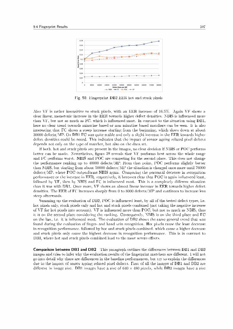
9.4 Fingerprint Results 107
�
����
����
����
����
���
����
����
����
����
� ���� ����� ����� ����� ����� ����� ���� ����� ���� �����
��������������
����������������
�� � �� ��� ��
Fig. 58: Fingerprint DB2 EER hot and stuck pixels
Also VF is rather insensitive to stuck pixels, with an EER increase of 16.5%. Again VF shows aclear linear, monotonic increase in the EER towards higher defect densities. NBIS is in�uenced morethan VF, but not as much as FC, which is in�uenced most. In contrast to the situation using DB1,here no clear trend towards minutiae based or non minutiae based matchers can be seen. It is alsointeresting that FC shows a steep increase starting from the beginning, which slows down at about30000 defects/MP. On DB1 FC was quite stable and only a slight increase in the EER towards higherdefect densities could be noted. This indicates that the impact of sensor ageing related pixel defectsdepends not only on the type of matcher, but also on the data set.
If both, hot and stuck pixels are present in the images, no clear decision if NBIS or POC performsbetter can be made. Nevertheless, �gure 58 reveals that VF performs best across the whole rangeand FC performs worst. NBIS and POC are competing for the second place. This does not changethe performance ranking up to 40000 defects/MP. From that point, POC performs slightly betterthan NBIS, but starting from about 50000 defects/MP the situation is changed once more until 76000defects/MP, where POC outperforms NBIS again. Comparing the percental decrease in recognitionperformance or the increase in EER, respectively, it becomes clear that POC is again in�uenced least,followed by VF, then by NBIS and FC is in�uenced most. This is a completely di�erent situationthan it was with DB1. Once more, VF shows an almost linear increase in EER towards higher defectdensities. The EER of FC increases sharply from 0 to 8000 defects/MP and continues to increase lesssteep afterwards.
Summing up the evaluation of DB2, POC is in�uenced least, by all of the tested defect types, i.e.hot pixels only, stuck pixels only and hot and stuck pixels combined (not taking the negative increaseof VF for hot pixels into account). VF is in�uenced more than POC, but not as much as NBIS, thusit is on the second place considering the ranking. Consequently, NBIS is on the third place and FCon the last, i.e. it is in�uenced most. The evaluation of DB2 shows the same general trend that wasfound during the evaluation of �nger- and hand vein recognition. Hot pixels cause the least decreasein recognition performance, followed by hot and stuck pixels combined, which cause a higher decreaseand stuck pixels only cause the highest decrease in recognition performance. This is in contrast toDB1, where hot and stuck pixels combined lead to the most severe e�ects.
Comparison between DB1 and DB2 This paragraph outlines the di�erences between DB1 and DB2images and tries to infer why the evaluation results of the �ngerprint matchers are di�erent. I will notgo into detail why there are di�erences in the baseline performances, but try to explain the di�erencesdue to the impact of sensor ageing related pixel defects. First of all the images of DB1 and DB2 aredi�erent in image size. DB1 images have a size of 640 × 480 pixels, while DB2 images have a size
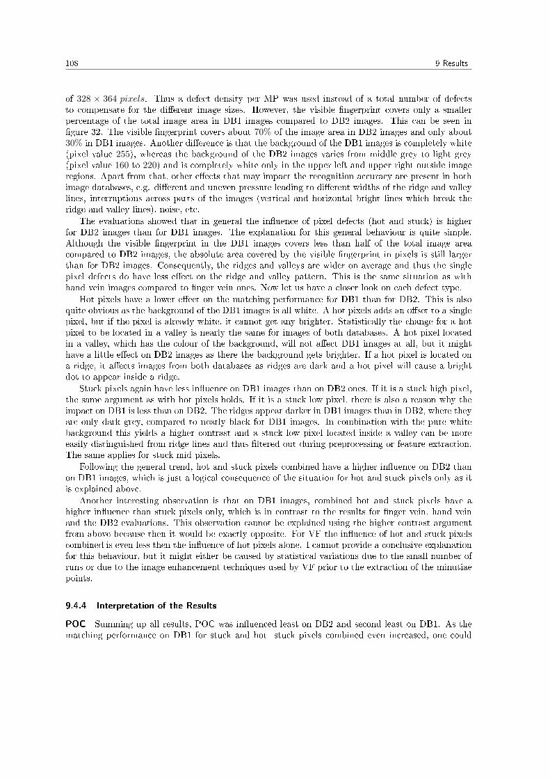
108 9 Results
of 328 × 364 pixels. Thus a defect density per MP was used instead of a total number of defectsto compensate for the di�erent image sizes. However, the visible �ngerprint covers only a smallerpercentage of the total image area in DB1 images compared to DB2 images. This can be seen in�gure 32. The visible �ngerprint covers about 70% of the image area in DB2 images and only about30% in DB1 images. Another di�erence is that the background of the DB1 images is completely white(pixel value 255), whereas the background of the DB2 images varies from middle grey to light grey(pixel value 160 to 220) and is completely white only in the upper left and upper right outside imageregions. Apart from that, other e�ects that may impact the recognition accuracy are present in bothimage databases, e.g. di�erent and uneven pressure leading to di�erent widths of the ridge and valleylines, interruptions across parts of the images (vertical and horizontal bright lines which break theridge and valley lines), noise, etc.
The evaluations showed that in general the in�uence of pixel defects (hot and stuck) is higherfor DB2 images than for DB1 images. The explanation for this general behaviour is quite simple.Although the visible �ngerprint in the DB1 images covers less than half of the total image areacompared to DB2 images, the absolute area covered by the visible �ngerprint in pixels is still largerthan for DB2 images. Consequently, the ridges and valleys are wider on average and thus the singlepixel defects do have less e�ect on the ridge and valley pattern. This is the same situation as withhand vein images compared to �nger vein ones. Now let us have a closer look on each defect type.
Hot pixels have a lower e�ect on the matching performance for DB1 than for DB2. This is alsoquite obvious as the background of the DB1 images is all white. A hot pixels adds an o�set to a singlepixel, but if the pixel is already white, it cannot get any brighter. Statistically the change for a hotpixel to be located in a valley is nearly the same for images of both databases. A hot pixel locatedin a valley, which has the colour of the background, will not a�ect DB1 images at all, but it mighthave a little e�ect on DB2 images as there the background gets brighter. If a hot pixel is located ona ridge, it a�ects images from both databases as ridges are dark and a hot pixel will cause a brightdot to appear inside a ridge.
Stuck pixels again have less in�uence on DB1 images than on DB2 ones. If it is a stuck high pixel,the same argument as with hot pixels holds. If it is a stuck low pixel, there is also a reason why theimpact on DB1 is less than on DB2. The ridges appear darker in DB1 images than in DB2, where theyare only dark grey, compared to nearly black for DB1 images. In combination with the pure whitebackground this yields a higher contrast and a stuck low pixel located inside a valley can be moreeasily distinguished from ridge lines and thus �ltered out during preprocessing or feature extraction.The same applies for stuck mid pixels.
Following the general trend, hot and stuck pixels combined have a higher in�uence on DB2 thanon DB1 images, which is just a logical consequence of the situation for hot and stuck pixels only as itis explained above.
Another interesting observation is that on DB1 images, combined hot and stuck pixels have ahigher in�uence than stuck pixels only, which is in contrast to the results for �nger vein, hand veinand the DB2 evaluations. This observation cannot be explained using the higher contrast argumentfrom above because then it would be exactly opposite. For VF the in�uence of hot and stuck pixelscombined is even less then the in�uence of hot pixels alone. I cannot provide a conclusive explanationfor this behaviour, but it might either be caused by statistical variations due to the small number ofruns or due to the image enhancement techniques used by VF prior to the extraction of the minutiaepoints.
9.4.4 Interpretation of the Results
POC Summing up all results, POC was in�uenced least on DB2 and second least on DB1. As thematching performance on DB1 for stuck and hot+stuck pixels combined even increased, one could

9.4 Fingerprint Results 109
also say that POC was most insensitive on DB1, depending if sensitive means any change regardlessin which direction or it only means negative changes. POC uses a �ngerprint enhancement techniqueprior to feature extraction, which is designed to remove noise from the �ngerprint images. Thisenhancement technique may also suppress most of the spiky shot noise caused by defective pixels.This is not surprising as both, POC and FC have been designed to be used especially for low-qualityimages and in the end, sensor ageing related pixel defects are just a kind of noise. POC correlates theimages in the frequency domain which has some advantages like brightness invariance and immunityto noise. In addition, only a band limited version of the normalised cross spectrum is used, limitedin a way that only those regions that are related to �ngerprint data are contained in the spectrum.This additionally �lters out interfering high frequency components like shot noise. Therefore POC isintrinsically robust against sensor ageing related pixel defects.
FC On DB1 FC was least in�uenced by sensor ageing related pixel defects compared to the othermatchers, not taking into account that the performance of POC increased. On DB2 FC performedworst for stuck and combined hot and stuck pixels and is on the third place for hot pixels. FCuses a di�erent feature extraction strategy than POC. Unlike POC, which uses the global ridge andvalley structure of the entire �ngerprint, FC uses this structure in a more local manner. Local ridgeorientation and local ridge frequency are extracted and used during matching. Local structures arealways more prone to small distortions like noise than global ones, thus FC is more sensitive todefective pixels. FC uses a normalisation step prior to feature extraction to adjust the images havinga speci�c grey-level mean and variance. Especially stuck pixels have a high in�uence on the grey-levelmean and variance in certain image regions, thus this normalisation step is of course a�ected. Duringfeature extraction FC is based on a bank of Gabor �lters, which are tuned to be responsive to theridge and furrow structure of the �ngerprint only. Therefore the feature extraction may again reducethe impact of the defective pixels. FC and POC both use the same additional �ngerprint enhancementstrategy prior to feature extraction. As FC is in�uenced more than POC, this enhancement strategyis able to reduce the impact of defective pixels only to a certain extent. Nevertheless, FC is in somecases more robust against sensor ageing e�ects than pure minutiae based matchers like NBIS, as itperformed better on DB1 and on DB2 for hot pixels at least.
NBIS NBIS is a typical example of a minutiae based matcher. At �rst it generates a quality map toexclude image regions with low quality in the feature extraction step. Then a binarisation is appliedto the images, mainly using morphological operations. This is followed by the minutiae extraction andan additional �ltering of false minutiae. The remaining minutiae are then used during the matchingprocess. Minutia points can also be regarded as local image features and thus they are a�ected moreby pixel defects than global structures. This is con�rmed by the evaluations as NBIS is the mosta�ected matcher on DB1 and the second most a�ected one on DB2. NBIS does not use an additionalimage enhancement prior to binarisation. The defective pixels in combination with the morphologicaloperations used during binarisation of the input �ngerprint images may cause ridges to be interruptedand ridge ends to be connected to each other. As the sensor ageing related pixel defects only introduceshot noise, these image regions are not marked as bad quality in the �rst step and thus they are ofcourse included in the feature extraction stage. The altered ridges and valleys cause some minutiaepoints to disappear, while others may be arti�cially generated. This can be seen on the DB2 imageexample in �gure 52. These false minutia points may be �ltered out, but some of them will remainafter the �ltering step, which in�uences the matching scores. There will be more minutia points thatcannot be matched even for genuine matches, thus the genuine scores decrease, leading to more falsenegative matches.

110 9 Results
VF VF is another minutiae based matcher. As it is a commercial one, there are no details aboutthe principles behind the feature extraction and matching process available. The only thing I know isthat it uses some advanced image enhancement techniques prior to feature extraction which is surelyone of the reasons why it performed best during all the tests, on DB1 and also on DB2. On DB1 itis most robust against hot and stuck pixel defects combined and on DB2 its matching performanceeven increases if only hot pixels are present. This indicates that VF is really robust against hot pixeldefects. According to Neurotechnology, VF is able to deal with sweat pores that are naturally presentin �ngerprint images exhibiting a certain resolution. Especially hot pixels located on a ridge are verysimilar to sweat pores and thus VF should be able to deal with hot pixels.
9.4.5 Simulation Results with Templates aged
The following �gures 59, 60 and 61 and �gures 62, 63 and 64 show the results with templates agedagainst only probe images aged for NBIS and VF on DB1 and DB2, respectively.
Let us �rst have a look on VF. Although the percental increases of VF's EER on DB1 suggest thatVF TA is in�uenced more than VF, a closer look on the diagrams reveals that there is no clear trendvisible. Sometimes VF outperforms VF TA and sometimes the situation changes, except for combinedhot and stuck pixels starting from a defect density of 48000 defects/MP. There VF TA performs worsethan VF, i.e. VF is in�uenced more by the defective pixels if also the template images are aged thanif only the probe images are. But in general neither VF nor VF TA is in�uenced more compared tothe other. Investigating the results on DB2 reveals that again VF TA's percental rise of all the EERvalues is higher compared to VF, but again the diagrams show that there is no obvious trend visible.The two lines di�er only slightly and again sometimes VF TA is in�uenced more than VF and viceversa, except for stuck pixels only where VF TA performs slightly worse than VF across the wholerange. Thus I would say for VF there is no distinction if the templates are aged or not, because thematching performance does hardly change.
Now the focus is on NBIS. NBIS TA and NBIS perform equally for hot pixels on DB1. Althoughthe percental rise of the EER at 40000 defects/MP may suggest that NBIS TA performs worse, thediagram clearly shows that there is absolutely no trend visible. However for stuck and combinedhot+stuck pixels there is a trend visible. The diagrams and also the EER values show that NBIS TAperforms better than NBIS, which is in a way the expected behaviour. If the templates are aged, theimages will be more similar again and this should lead to improved matching results. Therefore NBISTA behaves as expected on DB1. On DB2 the situation is completely di�erent. For all three testeddefect types, i.e. hot pixels only, stuck pixels only and combined hot+stuck pixels, the EER valuesin table 9 indicate that NBIS clearly outperforms NBIS TA with an increasing defect density. This iscon�rmed by the �gures 62, 63 and 64. The question now is, why is NBIS TA in�uenced more thanNBIS? Once again a look into the scores distribution can help to answer this question. The scoresdistribution for NBIS and NBIS TA at a defect rate of 24000 stuck pixel defects/MP is shown in�gure 65a. It can be seen that again the impostor scores are shifted to the right towards the genuineones. Figure 65b shows the FAR and FRR. There it can be seen that the FAR of NBIS TA is highercompared to NBIS. Both reveals an increased number of false positive matches for NBIS TA with anincreasing defect density, which is the reason for the lower matching performance. Actually the sameargument that was used to explain the expected behaviour can be used to explain this behaviour. OnDB2 the lower contrast and darker background in combination with the stuck and hot pixels leads tomore ridge and valley structures that are arti�cially generated and appear in the binarised images asit was explained in Paragraph 9.4.3. These structures appear in each image present in the database.If these lead to false minutiae during feature extraction, these minutia points will also be extractedfrom each of the images. Consequently, this leads to lower matching scores as these minutiae canalways be matched. This lowers the genuine match scores but also the impostor scores and leads to

9.4 Fingerprint Results 111
Fig. 59: Fingerprint DB1 EER NBIS + VF TA hotpixels only
Fig. 60: Fingerprint DB1 EER NBIS + VF TAstuck pixels only
�
����
����
����
����
���
����
����
����
� ���� ����� ����� ����� ����� ����� ���� ����� ���� �����
��������������
����������������
�� � �� ���� ����� ��
Fig. 61: Fingerprint DB1 EER NBIS + VF TA hot + stuck pixels
more overlapping of the genuine and impostor scores distributions. Thus the number of false positivematches increases and as a result the matching performance drops.
9.4.6 Fingerprint Conclusion
The evaluations on DB1 and DB2 showed that the impact of sensor ageing related pixel defects doesnot only depend on the type of pixel defects and on the particular matcher, but also on the imagesitself. The in�uence on DB1 images is in general less then on DB2 images. This is also true for theexperiments with additional template ageing. On DB1 the behaviour is as expected, while on DB2 dueto the higher in�uence of defective pixels in general it is not. On DB1 the minutiae based matchers arein�uenced more than the non minutiae based ones, which can be explained by the fact that minutiapoints are local image features that are more a�ected by single pixel defects. On DB1 FC is in�uencedleast, followed by POC (if counting the positive in�uence just as in�uenced, else they would switchplaces), next is VF and NBIS is in�uenced most. The situation for DB2 is di�erent. There POCis in�uenced least, followed by VF and NBIS, whereas FC is in�uenced most. Thus no clear trend,if minutiae based matchers are in�uenced more or not, can be seen. The only thing which can beseen is that VF performed best in terms of its absolute EER values for both databases. Although thein�uence on DB2 is higher, having a look at the two least in�uenced matchers, the rise in their EERstill stays below 17% (for stuck pixels, it is even lower for hot ones). According to section 8.4.1 anddepending on the �ngerprint scanner used, a defect rate of 0.03 defects/year (for the U.are.U 4000B
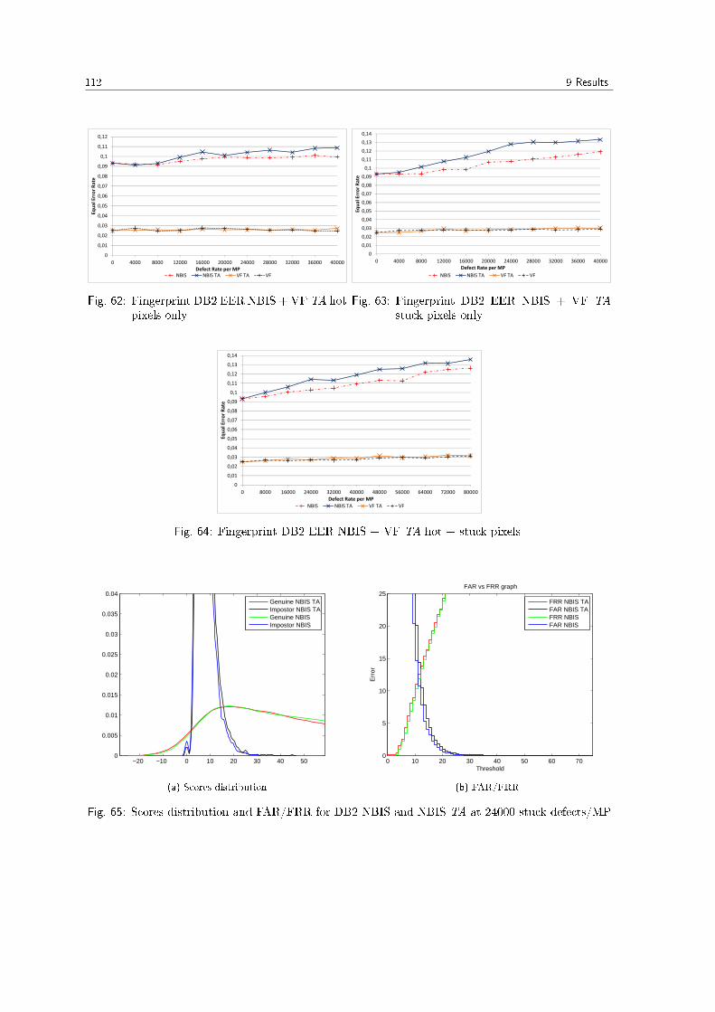
112 9 Results
�
����
����
����
����
����
����
���
���
����
���
����
����
� ���� ��� ����� ����� ����� ����� ���� ����� ����� �����
��������������
����������������
� �� � ����� ����� ��
Fig. 62: Fingerprint DB2 EER NBIS + VF TA hotpixels only
�
����
����
����
����
����
����
���
���
����
���
����
����
����
����
� ���� ��� ����� ����� ����� ����� ���� ����� ����� �����
��������������
����������������
� �� � ����� ����� ��
Fig. 63: Fingerprint DB2 EER NBIS + VF TAstuck pixels only
�
����
����
����
����
����
����
���
���
����
���
����
����
����
����
� ��� ����� ����� ����� ����� ���� ����� ����� ���� ����
��������������
����������������
� �� � ����� ����� ��
Fig. 64: Fingerprint DB2 EER NBIS + VF TA hot + stuck pixels
−20 −10 0 10 20 30 40 500
0.005
0.01
0.015
0.02
0.025
0.03
0.035
0.04
Genuine NBIS TAImpostor NBIS TAGenuine NBISImpostor NBIS
(a) Scores distribution
0 10 20 30 40 50 60 700
5
10
15
20
25
Threshold
Err
or
FAR vs FRR graph
FRR NBIS TAFAR NBIS TAFRR NBISFAR NBIS
(b) FAR/FRR
Fig. 65: Scores distribution and FAR/FRR for DB2 NBIS and NBIS TA at 24000 stuck defects/MP

9.4 Fingerprint Results 113
scanner) would occur. Statistically, this not even leads to a single defective pixel during a period of30 years. Despite FC showing a steep rise in its EER starting from a low number of defects on DB2for stuck and hot+stuck pixels combined, all other tested matchers only show a slight rise or even adecrease for a low number of defects. Stuck pixels are not reported to occur in real world applications.Furthermore, there would not be a single defective pixel and even if there are up to 100 pixel defects,the in�uence on the recognition accuracy is not worth mentioning. Following the trend of �nger andhand vein recognition, sensor ageing is not an issue in �ngerprint recognition systems.

114 9 Results

115
10 Summary
The main research topic of the present thesis was:
�Evaluating the impact of sensor ageing on the recognition accuracy of �nger image based biometricrecognition systems�.
According to my experimental results, there is no considerable in�uence on either of the testedschemes for a realistic number of defective pixels. In the following, I will give a short review of thepresent thesis at �rst and then I am going to conclude the evaluation results based on the di�erentbiometric traits, which are �nger veins, hand veins and �ngerprints to obtain this �nal statement. Iwill not go into details on each speci�c trait or any speci�c matcher once again as this was alreadydone in the corresponding subsection of the results section.
This thesis started with a short introduction on biometric recognition systems, widely used forauthentication purposes nowadays. Then the main impact of image sensor ageing, defective pixels,were described, followed by a quick overview over the existing literature regarding sensor ageing.Despite extensive literature research, by the time of writing this thesis, no literature could be foundregarding the impact of sensor ageing on the recognition accuracy of biometric recognition systems.This lead to the main topic of the present thesis:
To be able to evaluate solely the impact of sensor ageing, the pixel defects had to be simulated, i.e.the images were arti�cially �aged�. This procedure was selected in order to make sure that no otherin�uences than sensor ageing related pixel defects are present in the images and thus a�ect the results.In the scope of the evaluations, �ngerprint, �nger vein and hand vein based feature extraction andmatching schemes were evaluated: Two minutiae based �ngerprint matcher, one ridge feature basedmatcher and one correlation based matcher for �ngerprints, 5 binarisation type and one keypointbased approach for �nger veins and 3 binarisation type and 1 keypoint based approach for hand veins.All evaluations were conducted using some well established data sets as ground truth and then ageingthe images using the proposed ageing simulation algorithm. Usually only the probe images were aged,but in addition some experiments were conducted with aged template images one more time.
After the introductory section there was a short section about image sensors and their functionalprinciples, to be able to explain the ageing related e�ects, which were described in the next section then.This section not only stated the di�erent types of defects, it also mentioned some defect identi�cationtechniques and outlined the impact of di�erent sensor parameters on the defect growth rate. Section4 described several defect detection algorithms, which can be used to estimate the defect growth rateand the defect parameters from real world images. Section 5 explained the ageing simulation algorithmused to create the defect matrices and embed the pixel defects into the images.
Section 6 was about �ngerprint recognition and also reviewed some general principles of biometricrecognition systems. Besides �ngerprint matchers also �nger- and hand vein ones were evaluated, thussection 7 dealt with �nger and hand vein recognition. Afterwards section 8 stated the experimentalsetup with the databases used for each biometric trait and the simulation settings which were estimatedusing an empiric formula. This was followed by a detailed analysis of the evaluation results, whichcan be found in section 9 and brings us �nally back to this conclusion.
During the experiments, �ngerprint, �nger vein and hand vein matchers were evaluated and theresults were analysed and interpreted. Each of the single results showed that for a realistic numberof defective pixels, i.e. a realistic defect rate, there is no impact on the recognition accuracy. Theestimated defect rates are between 0.03− 0.07 defects/year and would lead to 1− 2 defective pixelsover a reasonable long sensor lifetime of 30 years. The evaluations showed that for such a low numberof defective pixels none of the tested matchers was in�uenced.
There can be application scenarios where the defect rate is considerably higher. Pixel defects occurdue to cosmic ray radiation, which is dependent on the altitude and and can lead to a pixel defect ratethat is up to 300 times higher during transatlantic �ights than on the ground. Such a scenario would

116 10 Summary
be a biometric authentication system for air plane pilots. Then there could be up to 600 defects perimage.
The evaluations showed that particular matchers are in�uenced by defective pixels due to sensorageing, not only negatively but also positively. In general the in�uence is again negligible even upto 10000 defects per image for some of the tested schemes. This clearly shows that most featureextraction and matching schemes are quite robust against these single pixel defects, although they arenot completely insensitive.
For �nger veins a simple denoising �lter was tested and the results showed that it is able toeliminate the impact of sensor ageing induced pixel defects almost completely at the cost of a slightlydecreased baseline performance. If sensor ageing related pixel defects become a problem, such a simpledenoising �lter can be used to suppress the impact on the recognition performance. Although it wasneither tested for hand vein recognition nor for �ngerprints it is not far-fetched that denoising wouldfurther mitigate the in�uence of sensor ageing on these biometric recognition systems. If a simpledenoising �lter is really able to cancel out the in�uence of the defective pixels caused by sensor ageingon �ngerprint and hand vein based recognition systems, will be part of my future work.
Referring back to the main question of this thesis I can now conclude that sensor ageing hasno impact at all on real world applications of �nger image based biometric recognition systems.Consequently, most state of the art �ngerprint, �nger- and hand vein recognition systems are alreadyable to deal with the level of defective pixels caused by sensor ageing during every day operation, i.e.they are already robust against sensor ageing related pixel defects.
Yet another interesting research question would be if there is a noticeable impact due to sensorageing related e�ects on non-optical biometric sensors, e.g. thermal �ngerprint sensors. Therefore,at �rst the ageing processes on these sensors have to be studied. Afterwards a suitable defect modelbased on the ageing related e�ects has to be found, which can then be used in a simulation to evaluatethe impact on the recognition accuracy like it was done for optical sensors during this work.

References 117
References
[1] Eui Chul Lee, Hyeon Chang Lee, and Kang Ryoung Park. Finger vein recognition using minutia-based alignment and local binary pattern-based feature extraction. International Journal ofImaging Systems and Technology, 19(3):179�186, 2009.
[2] Beining Huang, Yanggang Dai, Rongfeng Li, Darun Tang, and Wenxin Li. Finger-vein authen-tication based on wide line detector and pattern normalization. In Pattern Recognition (ICPR),2010 20th International Conference on, pages 1269�1272. IEEE, 2010.
[3] Albert JP Theuwissen. In�uence of terrestrial cosmic rays on the reliability of ccd image sensors-part 1: Experiments at room temperature. Electron Devices, IEEE Transactions on, 54(12):3260�3266, 2007.
[4] Albert JP Theuwissen. In�uence of terrestrial cosmic rays on the reliability of ccd imagesensors-part 2: Experiments at elevated temperature. Electron Devices, IEEE Transactions on,55(9):2324�2328, 2008.
[5] Glenn H Chapman, Jenny Leung, Israel Koren, and Zahava Koren. Tradeo�s in imager designwith respect to pixel defect rates. In Defect and Fault Tolerance in VLSI Systems (DFT), 2010IEEE 25th International Symposium on, pages 231�239. IEEE, 2010.
[6] Glenn H Chapman, Jenny Leung, Ana Namburete, Israel Koren, and Zahava Koren. Predictingpixel defect rates based on image sensor parameters. In Defect and Fault Tolerance in VLSI andNanotechnology Systems (DFT), 2011 IEEE International Symposium on, pages 408�416. IEEE,2011.
[7] Glenn H Chapman, Israel Koren, and Zahava Koren. Do more camera pixels result in a betterpicture? In On-Line Testing Symposium (IOLTS), 2012 IEEE 18th International, pages 73�78.IEEE, 2012.
[8] Glenn H Chapman, Jenny Leung, Rohit Thomas, Ana Namburete, Zahava Koren, and IsraelKoren. Projecting the rate of in-�eld pixel defects based on pixel size, sensor area, and iso.In IS&T/SPIE Electronic Imaging, pages 82980E�82980E. International Society for Optics andPhotonics, 2012.
[9] Glenn H Chapman, Rohit Thomas, Zahava Koren, and Israel Koren. Empirical formula for ratesof hot pixel defects based on pixel size, sensor area, and iso. In IS&T/SPIE Electronic Imaging,pages 86590C�86590C. International Society for Optics and Photonics, 2013.
[10] Jozsef Dudas, Cory Jung, Linda Wu, Glenn H Chapman, Israel Koren, and Zahava Koren. On-line mapping of in-�eld defects in image sensor arrays. In Defect and Fault Tolerance in VLSISystems, 2006. DFT'06. 21st IEEE International Symposium on, pages 439�447. IEEE, 2006.
[11] Jozsef Dudas, Cory Jung, Glenn H Chapman, Zahava Koren, and Israel Koren. Robust detectionof defects in imaging arrays. In Electronic Imaging 2006, pages 60590X�60590X. InternationalSociety for Optics and Photonics, 2006.
[12] Jozsef Dudas, Linda M Wu, Cory Jung, Glenn H Chapman, Zahava Koren, and Israel Koren.Identi�cation of in-�eld defect development in digital image sensors. In Electronic Imaging 2007,pages 65020Y�65020Y. International Society for Optics and Photonics, 2007.

118 References
[13] Jenny Leung, Jozsef Dudas, Glenn H Chapman, Israel Koren, and Zahava Koren. Quantitativeanalysis of in-�eld defects in image sensor arrays. In Defect and Fault-Tolerance in VLSI Systems,2007. DFT'07. 22nd IEEE International Symposium on, pages 526�534. IEEE, 2007.
[14] Jenny Leung, Glenn H Chapman, Israel Koren, and Zahava Koren. Automatic detection of in-�eld defect growth in image sensors. In Defect and Fault Tolerance of VLSI Systems, 2008.DFTVS'08. IEEE International Symposium on, pages 305�313. IEEE, 2008.
[15] Jenny Leung, Jozsef Dudas, Glenn H Chapman, Zahava Koren, and Israel Koren. Characterizationof pixel defect development during digital imager lifetime. In Electronic Imaging 2008, pages68160A�68160A. International Society for Optics and Photonics, 2008.
[16] Jenny Leung, Glenn H Chapman, Zahava Koren, and Israel Koren. Statistical identi�cationand analysis of defect development in digital imagers. In IS&T/SPIE Electronic Imaging, pages72500W�72500W. International Society for Optics and Photonics, 2009.
[17] Jenny Leung, Glenn H Chapman, Yong H Choi, Rohit Thomas, Zahava Koren, and Israel Koren.Analyzing the impact of iso on digital imager defects with an automated defect trace algorithm.In Proc. SPIE, volume 7536, page 75360F, 2010.
[18] Jessica Fridrich. Sensor defects in digital image forensic. In Digital Image Forensics, pages179�218. Springer, 2013.
[19] Jenny Leung, Glenn H Chapman, Israel Koren, and Zahava Koren. Characterization of gainenhanced in-�eld defects in digital imagers. In Defect and Fault Tolerance in VLSI Systems,2009. DFT'09. 24th IEEE International Symposium on, pages 155�163. IEEE, 2009.
[20] Jozsef Dudas. Characterization and avoidance of in-�eld defects in solid-state image sensors.PhD thesis, SIMON FRASER UNIVERSITY, 2008.
[21] Jenny Leung. Measurement and analysis of defect development in digital imagers. PhD thesis,Applied Science: School of Engineering Science, 2011.
[22] Thomas Bergmüller, Luca Debiasi, Andreas Uhl, and Zhenan Sun. Impact of sensor ageing oniris recognition. In Proceedings of the IAPR/IEEE International Joint Conference on Biometrics(IJCB'14), 2014.
[23] Albert JP Theuwissen. In�uence of terrestrial cosmic rays on the reliability of ccd image sensors.In Electron Devices Meeting, 2005. IEDM Technical Digest. IEEE International, pages 811�814.IEEE, 2005.
[24] Byoungjae Jin, Nohpill Park, Kayikkalthop M George, Minsu Choi, and Mark B Yeary. Mod-eling and analysis of soft-test/repair for ccd-based digital x-ray systems. Instrumentation andMeasurement, IEEE Transactions on, 52(6):1713�1721, 2003.
[25] G.H. Chapman, I Koren, Z. Koren, J. Dudas, and C. Jung. On-line identi�cation of faults infault-tolerant imagers. In Defect and Fault Tolerance in VLSI Systems, 2005. DFT 2005. 20thIEEE International Symposium on, pages 149�157, Oct 2005.
[26] Davide Maltoni, Dario Maio, Anil K Jain, and Salil Prabhakar. Handbook of �ngerprint recogni-tion. springer, 2009.
[27] Pietro Coli. Vitality detection in personal authentication systems using �ngerprints. 2008.

References 119
[28] Hiroshi NAKAJIMA, Koji KOBAYASHI, and Tatsuo HIGUCHI. A �ngerprint matching al-gorithm using phase-only correlation. IEICE Transactions on Fundamentals of Electronics, Com-munications and Computer Sciences, 87(3):682�691, 2004.
[29] Lin Hong, Yifei Wan, and Anil Jain. Fingerprint image enhancement: algorithm and performanceevaluation. Pattern Analysis and Machine Intelligence, IEEE Transactions on, 20(8):777�789,1998.
[30] Anil K Jain, Salil Prabhakar, Lin Hong, and Sharath Pankanti. Filterbank-based �ngerprintmatching. Image Processing, IEEE Transactions on, 9(5):846�859, 2000.
[31] Ra�aele Cappelli, Matteo Ferrara, and Davide Maltoni. Minutia cylinder-code: A new rep-resentation and matching technique for �ngerprint recognition. Pattern Analysis and MachineIntelligence, IEEE Transactions on, 32(12):2128�2141, 2010.
[32] Barclays UK. Barclays newsroom, �rst in uk to lauch new biometric reader for cus-tomers. http://www.newsroom.barclays.com/Press-releases/Barclays-first-in-UK-to-
launch-new-Biometric-Reader-for-customers-bab.aspx, June 2014. [Online; accessed 19-June-2014].
[33] B.T. Ton and R.N.J. Veldhuis. A high quality �nger vascular pattern dataset collected using acustom designed capturing device. In International Conference on Biometrics, ICB 2013. IEEE,2013.
[34] Jianjun Zhao, Hogliang Tian, Weixing Xu, and Xin Li. A new approach to hand vein imageenhancement. In Intelligent Computation Technology and Automation, 2009. ICICTA'09. SecondInternational Conference on, volume 1, pages 499�501. IEEE, 2009.
[35] Jing Zhang and Jinfeng Yang. Finger-vein image enhancement based on combination of gray-level grouping and circular gabor �lter. In Information Engineering and Computer Science, 2009.ICIECS 2009. International Conference on, pages 1�4. IEEE, 2009.
[36] B. Ton . Vascular patern of the �nger: biometric of the future? sensor design, data collectionand performance veri�cation, July 2012.
[37] Naoto Miura, Akio Nagasaka, and Takafumi Miyatake. Extraction of �nger-vein patterns usingmaximum curvature points in image pro�les. IEICE transactions on information and systems,90(8):1185�1194, 2007.
[38] Naoto Miura, Akio Nagasaka, and Takafumi Miyatake. Feature extraction of �nger-vein patternsbased on repeated line tracking and its application to personal identi�cation. Machine Visionand Applications, 15(4):194�203, 2004.
[39] Nobuyuki Otsu. A threshold selection method from gray-level histograms. Automatica, 11(285-296):23�27, 1975.
[40] David G Lowe. Object recognition from local scale-invariant features. In Computer vision, 1999.The proceedings of the seventh IEEE international conference on, volume 2, pages 1150�1157.Ieee, 1999.
[41] Herbert Bay, Tinne Tuytelaars, and Luc Van Gool. Surf: Speeded up robust features. In ComputerVision�ECCV 2006, pages 404�417. Springer, 2006.
[42] Andreas Uhl and Y Holler. Iris-sensor authentication using camera prnu �ngerprints. In Biomet-rics (ICB), 2012 5th IAPR International Conference on, pages 230�237. IEEE, 2012.

120 References
[43] Dario Maio, Davide Maltoni, Ra�aele Cappelli, Jim L Wayman, and Anil K Jain. Fvc2004: Third�ngerprint veri�cation competition. In Biometric Authentication, pages 1�7. Springer, 2004.
[44] Jessica Fridrich. Digital image forensics. Signal Processing Magazine, IEEE, 26(2):26�37, 2009.
[45] Gayathri G Nampoothiri and Albert JP Theuwissen. Investigating the ageing e�ects on imagesensors due to terrestrial cosmic radiation.
[46] Yap-Peng Tan and T. Acharya. A robust sequential approach for the detection of defective pixelsin an image sensor. In Acoustics, Speech, and Signal Processing, 1999. Proceedings., 1999 IEEEInternational Conference on, volume 4, pages 2239�2242 vol.4, Mar 1999.
[47] Javier Alda et al. Bad pixel identi�cation by means of principal components analysis. Opticalengineering, 41(9):2152�2157, 2002.
[48] Christof Kauba, Jakob Reissig, and Andreas Uhl. Pre-processing cascades and fusion in �ngervein recognition. In Proceedings of the International Conference of the Biometrics Special InterestGroup (BIOSIG'14), Darmstadt, Germany, September 2014.
[49] Karel Zuiderveld. Contrast limited adaptive histogram equalization. In Graphics gems IV, pages474�485. Academic Press Professional, Inc., 1994.
[50] Olympus America Inc. Building a charge-coupled device. http://olympusmicro.com/primer/
java/digitalimaging/ccd/virtual2/index.html, June 2014. [Online; accessed 19-June-2014].
[51] National Institute of Standards and Technology (NIST). Nist biometric image software (nbis).http://fingerprint.nist.gov/NBIS/, June 2014. [Online; accessed 19-June-2014].
[52] Neurotechnology. Veri�nger 7.0 sdk. http://www.neurotechnology.com/download.html#
verifinger_sdk_trial, June 2014. [Online; accessed 19-June-2014].
[53] Anouar Ben Khalifa, Sami Gazzah, and Najoua Essoukri BenAmara. Adaptive score normaliz-ation: A novel approach for multimodal biometric systems. International Journal of Computer,Information Science and Engineering, 7:18�26, 2013.
[54] EC Lee and KR Park. Restoration method of skin scattering blurred vein image for �nger veinrecognition. Electronics letters, 45(21):1074�1076, 2009.
[55] Jialiang Peng, Ning Wang, Ahmed A Abd El-Latif, Qiong Li, and Xiamu Niu. Finger-veinveri�cation using gabor �lter and sift feature matching. In Intelligent Information Hiding andMultimedia Signal Processing (IIH-MSP), 2012 Eighth International Conference on, pages 45�48.IEEE, 2012.