Embed Size (px)
Citation preview
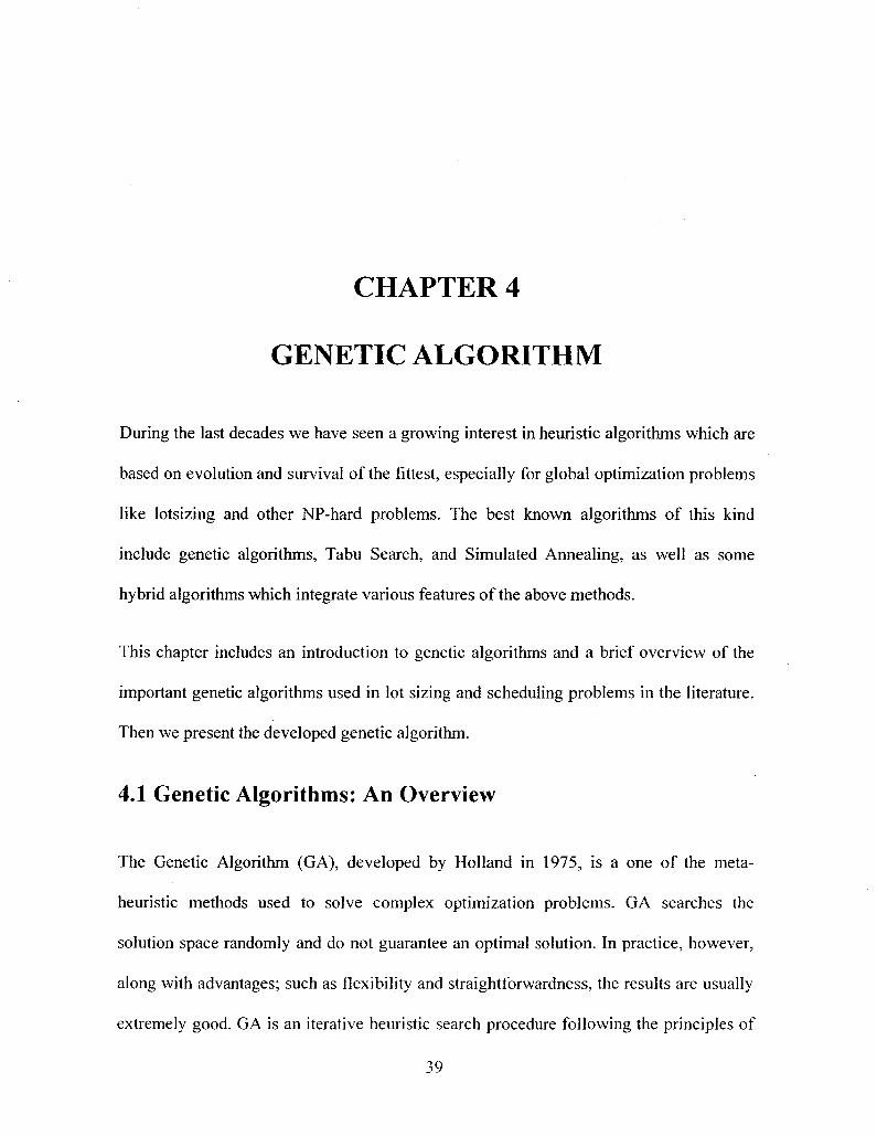
Integrating Capacitated Lot-Sizing and Lot Streaming In Flowshop Schedules
with Time Varying Demand
Alipasha Bayat
A Thesis
in
The Department
of
Mechanical and Industrial Engineering
Presented in Partial Fulfillment of the Requirements for the Degree of Master of Applied Science (Industrial Engineering) at
Concordia University Montreal, Quebec, Canada
December 2008
© Alipasha Bayat, 2008
1*1 Library and Archives Canada
Published Heritage Branch
395 Wellington Street Ottawa ON K1A 0N4 Canada
Bibliotheque et Archives Canada
Direction du Patrimoine de I'edition
395, rue Wellington OttawaONK1A0N4 Canada
Your file Votre reference ISBN: 978-0-494-63294-9 Our file Notre reference ISBN: 978-0-494-63294-9
NOTICE: AVIS:
The author has granted a nonexclusive license allowing Library and Archives Canada to reproduce, publish, archive, preserve, conserve, communicate to the public by telecommunication or on the Internet, loan, distribute and sell theses worldwide, for commercial or noncommercial purposes, in microform, paper, electronic and/or any other formats.
L'auteur a accorde une licence non exclusive permettant a la Bibliotheque et Archives Canada de reproduire, publier, archiver, sauvegarder, conserver, transmettre au public par telecommunication ou par I'lnternet, preter, distribuer et vendre des theses partout dans le monde, a des fins commerciales ou autres, sur support microforme, papier, electronique et/ou autres formats.
The author retains copyright ownership and moral rights in this thesis. Neither the thesis nor substantial extracts from it may be printed or otherwise reproduced without the author's permission.
L'auteur conserve la propriete du droit d'auteur et des droits moraux qui protege cette these. Ni la these ni des extraits substantiels de celle-ci ne doivent etre imprimes ou autrement reproduits sans son autorisation.
In compliance with the Canadian Privacy Act some supporting forms may have been removed from this thesis.
Conformement a la loi canadienne sur la protection de la vie privee, quelques formulaires secondaires ont ete enleves de cette these.
While these forms may be included in the document page count, their removal does not represent any loss of content from the thesis.
Bien que ces formulaires aient inclus dans la pagination, il n'y aura aucun contenu manquant.
1+1
Canada
ABSTRACT
Integrating Capacitated Lot-Sizing and Lot Streaming In Flowshop
Schedules with Time Varying Demand
Alipasha Bayat
Any reasonable production planning contains three important decisions on lot size, lead
time, and capacity. The common approach in the literature is to divide the planning
problem into lot sizing, lot sequencing, and lot splitting sub-problems. Very few studies,
to the best of our knowledge, have been conducted on the interdependencies and three-
way interaction of lead-time, lot size, and actual capacity usage. A particular lot size
calculated by the sub-problem method, however, will likely yield an infeasible solution or
at least result in schedule instability (nervousness). This is just because in most
capacitated lot sizing models, the capacity constraints in the model only take into
consideration the available time on each work station, ignoring the sequencing of lots,
sublot sizes, and their effect on makespan and lead times. In this thesis we bridge the gap
between lot sizing and scheduling in flowshops, and examine the use of the lot splitting
and sequencing techniques to reduce schedule instability. A mixed integer programming
formulation is presented, which enables us to simultaneously find the optimal lot sizes as
well as the corresponding sublot sizes and sequence of jobs. With this model, small size
problems can be solved within a reasonable time. The computational results confirm that
this model can be advantageous in dampening the scheduling nervousness. For larger size
instances, a Genetic algorithm is proposed.
iii

Acknowledgements
This thesis is dedicated to the memory of my beloved father and to my mother, Maliheh,
for her love and support throughout my life. As always, I am deeply grateful to her.
I would like to express my sincere gratitude to my supervisor, Professor Dr. Akif Asil
Bulgak, for his patience, kindness, constructive comments, and for his general support
throughout this work. I appreciate all that you did for me and I will miss working with
you very much.
Special thanks to my friend Mohammad Jabbari Hagh for his many hours of assistance
with programming and for all I have learned from him.
I must extend my thanks to Dr. Fantahun Defersha and also to my friends and colleagues
Iman Niroomand and Amir Khataie for our academic discussions.
IV
Table of Contents
List of Figures vii
List of Tables viii
List of Acronyms ix
CHAPTER 1 INTRODUCTION 1
1.1 Motivation 1
1.2 Objectives and Contributions 4
1.3 Overview of this Thesis 5
CHAPTER 2 LITERATURE REVIEW 6
2.1 Lot-Sizing 6
2.1.1 Simple and Common Sense Techniques 7
2.1.2 Exact Optimization Methods 7
2.1.3 Heuristics. 9
2.1.4 General Characteristics of Lot Sizing Problems 11
2.2 Scheduling (Sequencing and Lot-Streaming) 12
2.2.1 Notions and Classifications 15
2.2.2 Common Solution Methods 18
2.3 Integrated Lot-Sizing and Scheduling 21
2.4 Lead Time 27
CHAPTER 3 MATEMATICAL FORMULATION 29
3.1 Assumptions and Limitations 29
3.2 Notations 30
3.3 Mathematical Model 32
v
3.4 Computational Experiments 34
3.4.1 A Numerical Example 34
3.4.2 Analytical Examples 35
CHAPTER 4 GENETIC ALGORITHM 39
4.1 Genetic Algorithms: An Overview 39
4.1.1 GA Design Factors 41
4.1.2 GA Parameters 45
4.2 Proposed Genetic Algorithm 45
4.2.1 Chromosome Representation 46
4.2.2 Decoding Algorithm 48
4.2.3 Genetic Algorithm Procedure 53
4.2.4 Fitness Function Evaluation 54
4.2.5 Genetic Operators 55
4.2.6 Selection Mechanism. 56
4.3 Tuning GA Parameters 57
4.4 Computational Results 59
CHAPTER 5 CONCLUSIONS AND FUTURE WORK 62
Bibliography 65
APPENDIX 1: Classification of Lot Sizing Problems 71
APPENDIX 2: Classification of Lot Streaming Problems 72
APPENDIX 3: Lingo Code 73
APPENDIX 4: Decoding Algorithm Pseudo Code 75
APPENDIX 5: Genetic Algorithm Programming Code 76
vi
List of Figures
Figure 1 -1: Hierarchical Planning Approach 3
Figure 2-1: m-Machine Flowshop 13
Figure 2-2: Gantt Charts of Different sublot Sizes 17
Figure 2-3: The Integrated Framework of Scheduling System 24
Figure 3-1: Gantt Chart of Production in Month of March. 35
Figure 4-1: The GA Procedure 40
Figure 4-2: Chromosome for Single Item Lot Sizing 46
Figure 4-3: Chromosome for 3-Item Lot Sizing and Sequencing 47
Figure 4-4: Flowchart of Decoding Algorithm 50
Figure 4-5: Chromosome 3-Itemand 6 Periods 51
Figure 4-6: Global Genetic Algorithm 54
Figure 4-7: Crossover Operator 55
Figure 4-8: Selection Mechanism 57
Figure 4-9: Comparison between Lingo objective bound and GA objective value 61
vn
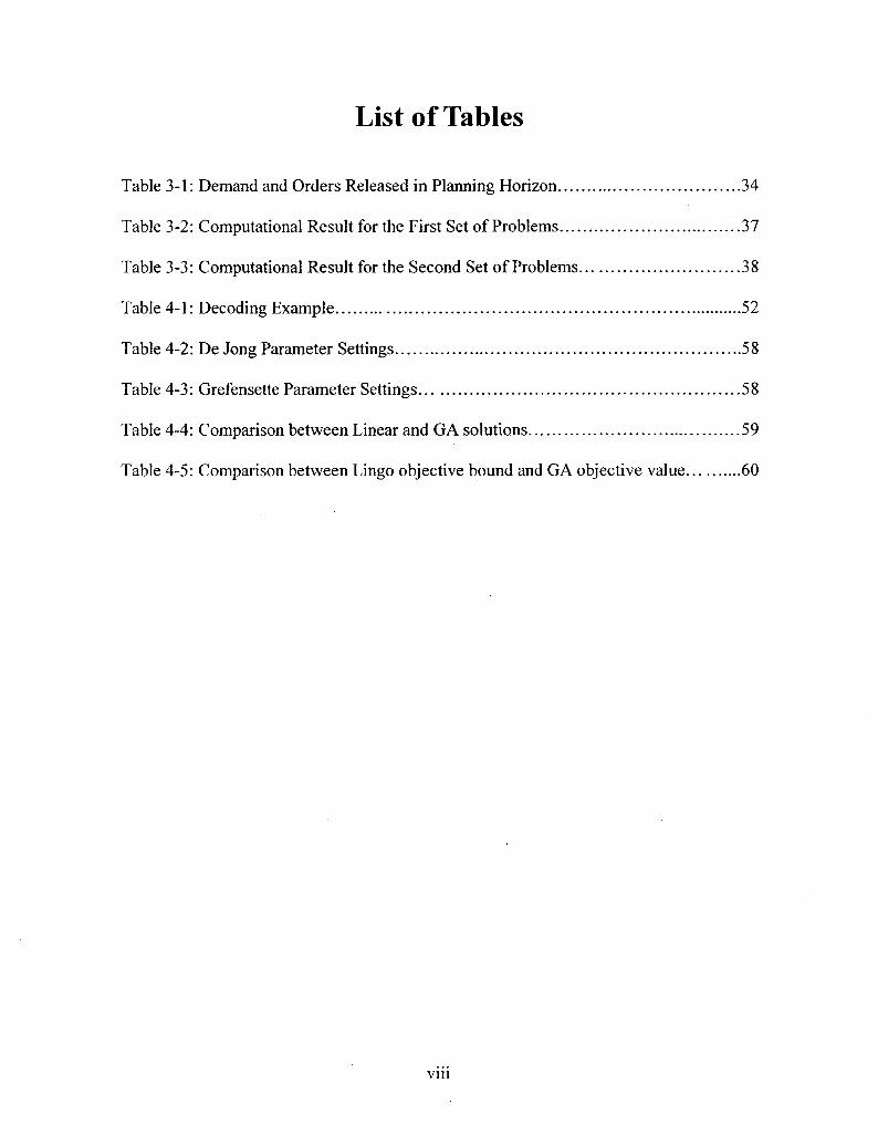
List of Tables
Table 3-1: Demand and Orders Released in Planning Horizon 34
Table 3-2: Computational Result for the First Set of Problems 37
Table 3 -3: Computational Result for the Second Set of Problems 38
Table 4-1: Decoding Example 52
Table 4-2: De Jong Parameter Settings 58
Table 4-3: Grefensette Parameter Settings 58
Table 4-4: Comparison between Linear and GA solutions 59
Table 4-5: Comparison between Lingo objective bound and GA objective value 60
V1I1
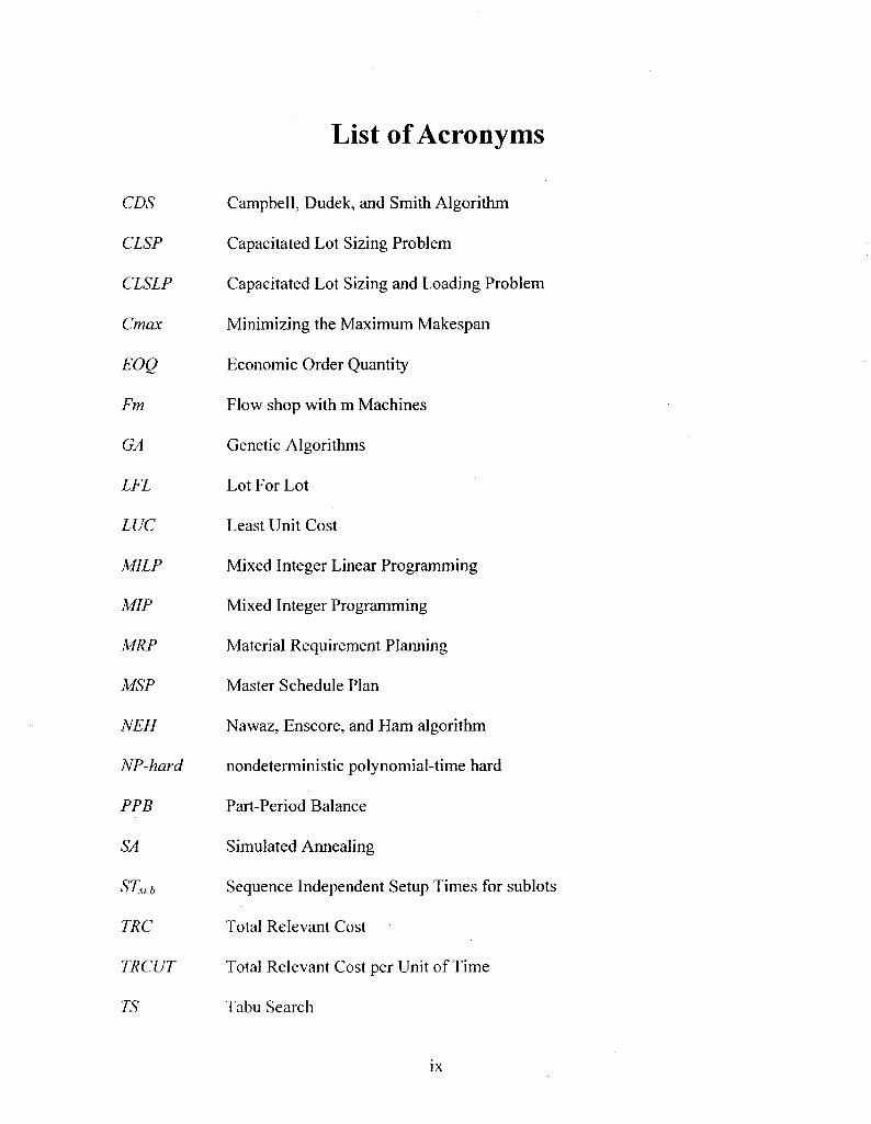
List of Acronyms
CDS
CLSP
CLSLP
Cmax
EOQ
Fm
GA
LFL
LUC
M1LP
MIP
MRP
MSP
NEH
NP-hard
PPB
SA
STsij,
TRC
TRCUT
TS
Campbell, Dudek, and Smith Algorithm
Capacitated Lot Sizing Problem
Capacitated Lot Sizing and Loading Problem
Minimizing the Maximum Makespan
Economic Order Quantity
Flow shop with m Machines
Genetic Algorithms
Lot For Lot
Least Unit Cost
Mixed Integer Linear Programming
Mixed Integer Programming
Material Requirement Planning
Master Schedule Plan
Nawaz, Enscore, and Ham algorithm
nondeterministic polynomial-time hard
Part-Period Balance
Simulated Annealing
Sequence Independent Setup Times for sublots
Total Relevant Cost
Total Relevant Cost per Unit of Time
Tabu Search
]X
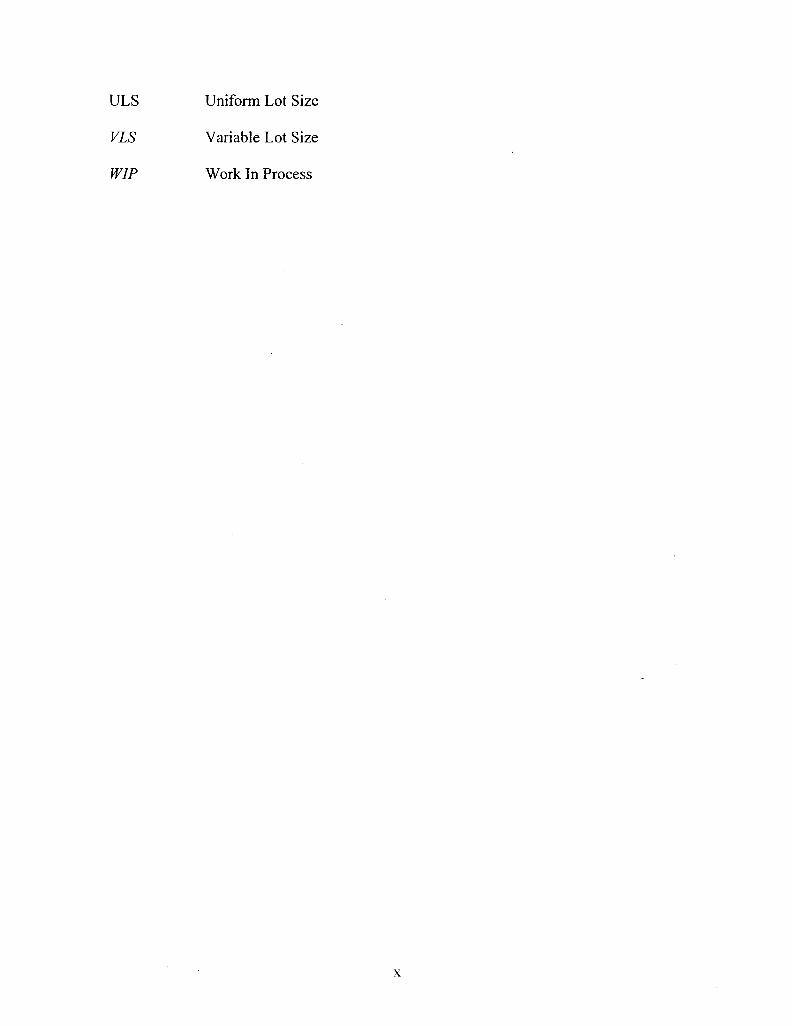
ULS Uniform Lot Size
VIS Variable Lot Size
W1P Work In Process
x
CHAPTER 1
INTRODUCTION
1.1 Motivation
The aim of lot-sizing research is to minimize setup and holding costs by determining
production lot size and inventory levels to meet a given demand. Lot streaming (Biskup
and Feldmann, 2006), on the other hand, aims to divide lots into sublots in order to allow
overlapping process in a multi-stage production system to accelerate the flow of material
and reduce the lead-time.
The common approach in the literature (known as the "hierarchical approach") is to
divide planning problem into lot sizing, lot splitting, and sequencing sub-problems. First,
using the master production plan, supported by bill of materials, and production structure,
the lot size for each product or part would be found. Then, after orders are released to
shop floor, lot splitting and sequencing techniques will be used to find the optimal
production sequence and sublot sizes. A particular lot size calculated by this common
practice might, however, gives an infeasible, or at least a poor solution in respect to other
aspects such as work in process (W1P), inventory holding cost, and set up costs. This
1
infeasibility forces the planner to frequently change the master production plan which
results in schedule instability (nervousness). This is because most capacitated lot sizing
models have four major unrealistic assumptions:
First, conventional capacitated lot sizing models, also known as CLSP, assume that the
time spent by each lot on each work center is small and negligible. This only makes
physical sense when a single item transfers from one work center to another (lots of size
one). However, when the production is by lots, the processing time of a lot depends on
the size of the lot and may not be negligible. For example, the time spent on machine 1
by a lot of "«" items with "i>" being the processing time is "n*P". Additionally, machine
2 would be idle for "n*P" units of time since the first job scheduled on machine 2 cannot
start until it is completed on machine 1. Thus, the capacity available for production
depends on the size of the production sublots.
Second, in most capacitated lot sizing models, the capacity constraints are nothing more
than the available time of each machine. Again, this assumption is only valid, if there is
zero idling time. In a flow shop in which production is done in lots, assuming zero idling
times means ignoring the effects of sequencing and sublot sizes, on makespan and lead
time.
Third, in presence of setup times, the limited capacity available for production may be
reduced by changeovers, causing sequence- dependent setup times. Lot sizing and
capacity usage therefore depend on both the sequence and the size of the sublots.
2
Fourth, conventional capacitated lot-sizing models consider the lead time as a fixed and
controllable input data, when it is really an output of other decisions, especially lot sizing
and sequencing (Lasserre, 2003).
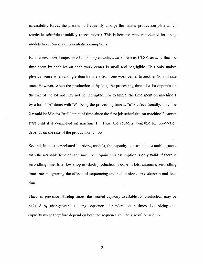
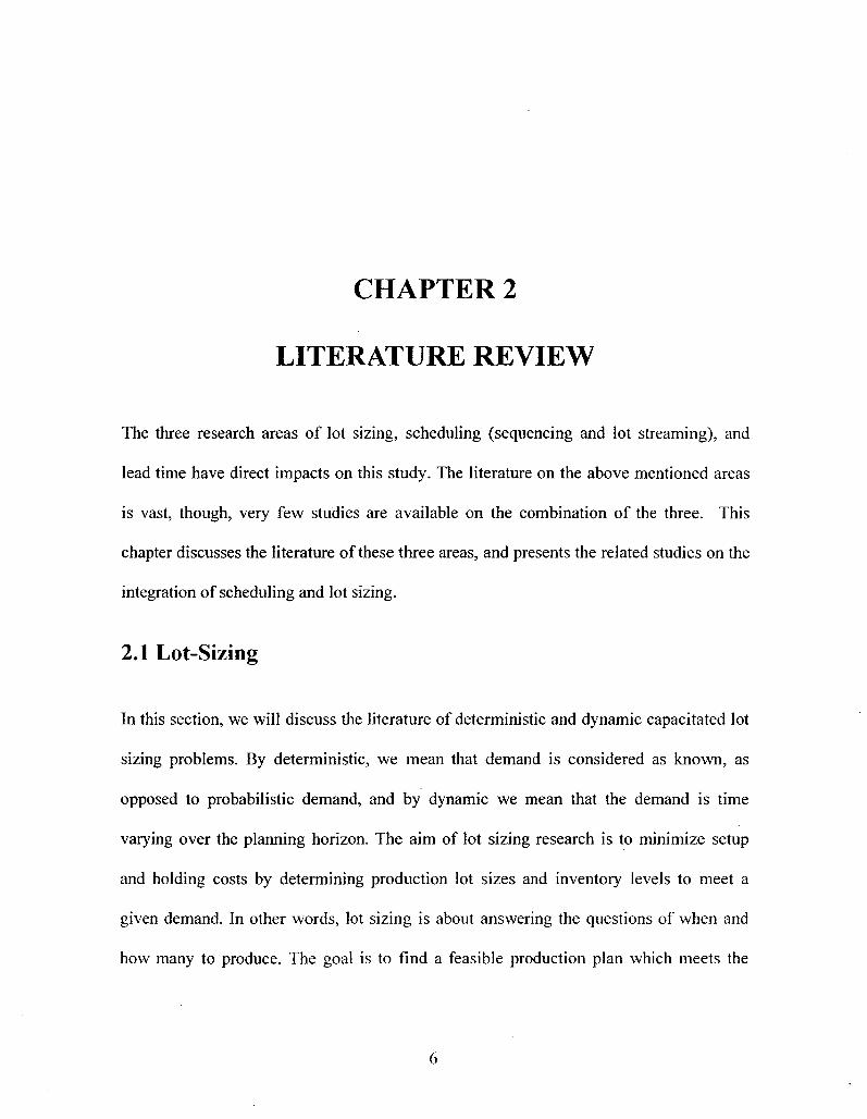
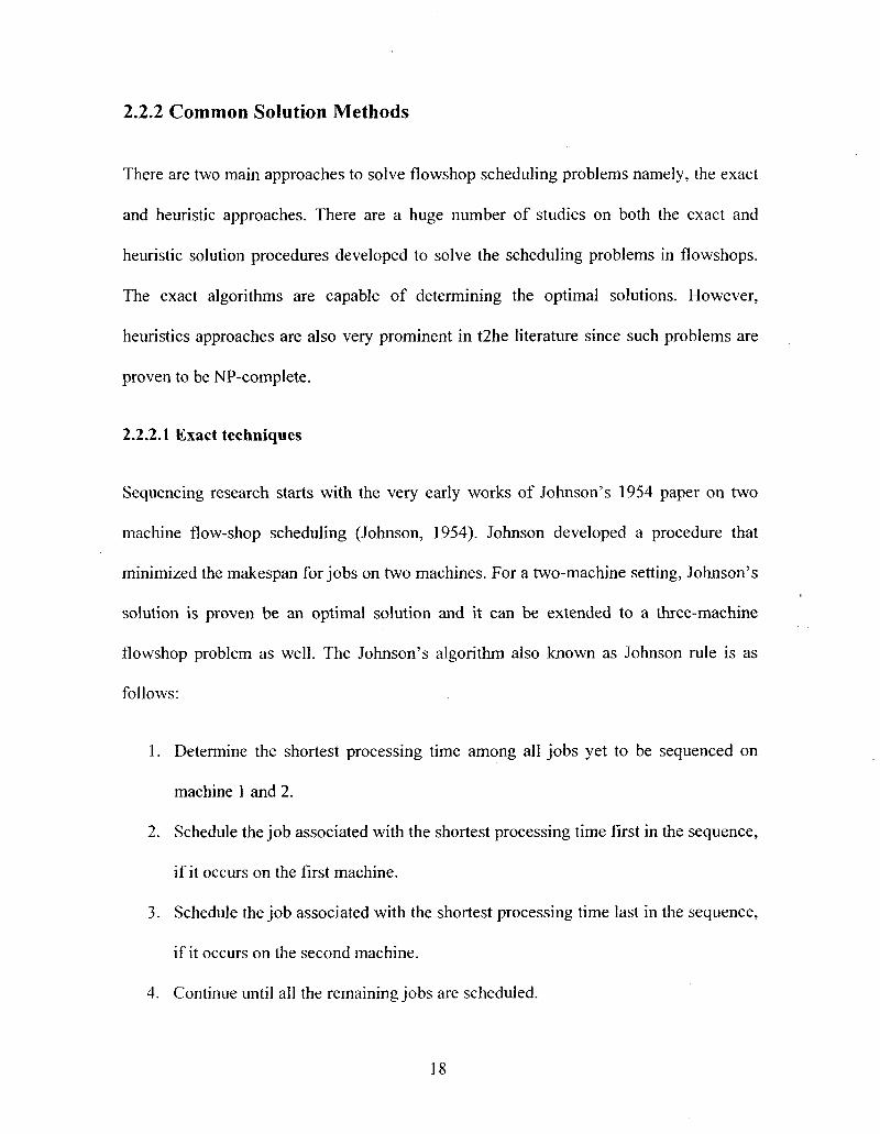
Capacity Planning
, ' *
K. N
Aggregate Production Planning
'' Master Production
Schedule
1' Material Planning
(Lot Sizing)
'' Scheduling
(Sequencing & splitting)
I J
J
>
[ j
Long term
Medium term
Short term
Figure 1-1: Hierarchical Planning Approach
Making any of the above assumptions would result in failure to plan capacity and in
scheduling instability. Scheduling instability is a severe problem in any production
planning system. It can be caused by one of the following reasons:
• Uncertain events occurring within or outside the production system such as
forecast errors and machine breakdowns,
• Operating factors such as lotsizing rules and capacity utilization
Traditionally, there are two options for dealing with instability: first to maintain safety
stock, safety lead time and safety capacity, and second to change the master production
schedule (MPS). There is a large cost associated with first option, and frequent
rescheduling leads to system instability.
Ho (1998) concluded that although forecast errors have impact on instability, use of an
appropriate lot sizing rule may neutralize the negative impact of forecast errors. He also
examined dampening effect of different lot sizing rules (Ho, 2005). He concluded that
part period balancing rule and least total cost rule turn out to be two effective lot sizing
rules to reduce system nervousness (Ho, 1986; Ho and Law, 1995; Ho, 2005).
1.2 Objectives and Contributions
In this thesis we focus on the problem of finding the optimal lot size for multiple items
with time varying demand in a multistage production system, when lot streaming and
sequencing are applied simultaneously to ensure order's feasibility and reduce the need
for rescheduling of the master production plan. The main contribution of this thesis is the
integration of sequencing and scheduling decisions with lot sizing. We make our decision
on the sequence of production and the sublot sizes simultaneously in advance, thus, we
have better schedule because we know the idling times of machines and we can fill them
with jobs. Moreover this can help us to have better estimate of the lead times. In order
achieve our goal we propose the following:
• Formulated the problem as a mixed integer linear programming problem model
• Developed a genetic algorithm (GA)
• Generated random problems to evaluate and compare the linear model and genetic
algorithm
4
1.3 Overview of this Thesis
Chapter 2 is an introduction to existing literature on the three subjects of lot sizing,
scheduling, and lead time. It introduces some of the works done on the integration of
these three subjects. This literature review focuses mainly on the flowshop problem.
Chapter 3 presents a mixed integer linear formulation of the problem. Later in Chapter 5
this exact solution will be used as a benchmark for evaluating the genetic algorithm.
Chapter 4 provides a study on design of genetic algorithms (GA), their design factors,
and their parameters. Then, it presents our proposed genetic algorithm to solve the lot
sizing problem (combined with scheduling) in more detail. It also presents numerical
examples and comparison with the exact solution presented in chapter 3 in order to
illustrate the efficiency of genetic algorithm.
Chapter 5 is the summary of this thesis and provides some direction for future research
works.
5
CHAPTER 2
LITERATURE REVIEW
The three research areas of lot sizing, scheduling (sequencing and lot streaming), and
lead time have direct impacts on this study. The literature on the above mentioned areas
is vast, though, very few studies are available on the combination of the three. This
chapter discusses the literature of these three areas, and presents the related studies on the
integration of scheduling and lot sizing.
2.1 Lot-Sizing
In this section, we will discuss the literature of deterministic and dynamic capacitated lot
sizing problems. By deterministic, we mean that demand is considered as known, as
opposed to probabilistic demand, and by dynamic we mean that the demand is time
varying over the planning horizon. The aim of lot sizing research is to minimize setup
and holding costs by determining production lot sizes and inventory levels to meet a
given demand. In other words, lot sizing is about answering the questions of when and
how many to produce. The goal is to find a feasible production plan which meets the
6
demand as stated in master schedule plan (MSP), while having the minimum setup and
inventory holding cost.
Based on the literature, solution methods of lot sizing problems can be classified into
three main categories: simple and common sense techniques, exact optimization methods,
and heuristic methods.
2.1.1 Simple and Common Sense Techniques
Lot sizing research began with simple techniques like EOQ, fixed order quantity, and lot
for lot (LFL) models and developed further to handle various cases. The EOQ model is
single level, single item production with no capacity constraints. The demand is
deterministic and assumed to have constant rate. EOQ model is a continuous time model
and it is very easy to solve. When the demand variation is small, we can ignore the time
variability of demand and use the basic EOQ model.
In the lot for lot method, which is considered to be the simplest method, order quantities
are the same as demand in each period. This it is not the best method when the setup cost
is high.
2.1.2 Exact Optimization Methods
The most cited optimization method for solving lotsizing problems is the Wagner-Whitin
algorithm, which uses integer or mixed programming. Development of the dynamic
method of Wagner-Whitin constitutes a major improvement in solving lot sizing
problems. Wagner-Whitin (Wagner, 1958) assumes a finite planning horizon which is
divided into discrete periods. Demand is time-varying and considered to be deterministic
7
and known for each period. But still it was un-capacitated and single level and a single
item problem.
The next generation of models is a combination of dynamic methods like Wagner-Whitin
and the capacity constraints, called the capacitated lot sizing problem (CLSP). Single
level lot-sizing problem is reviewed by many scholars. In the next sections, we present
the mathematical formulation and the basic assumptions of this model.
2.1.2.1 Assumptions and Limitations
To find the best amount and timing of production, following assumptions were made for
solving the single item capacitated lot sizing problem:
• The demand rate is known and deterministic,
• The cost factors do not change with time. In other words inflation is negligible
• No shortage is allowed
• The carrying cost is only applicable to the inventory that is carried over from one
period to the next period
• The production has to be completed at the end of each period to meet the demand
of the next period
• Jobs should be processed in sequence on m machines or stages
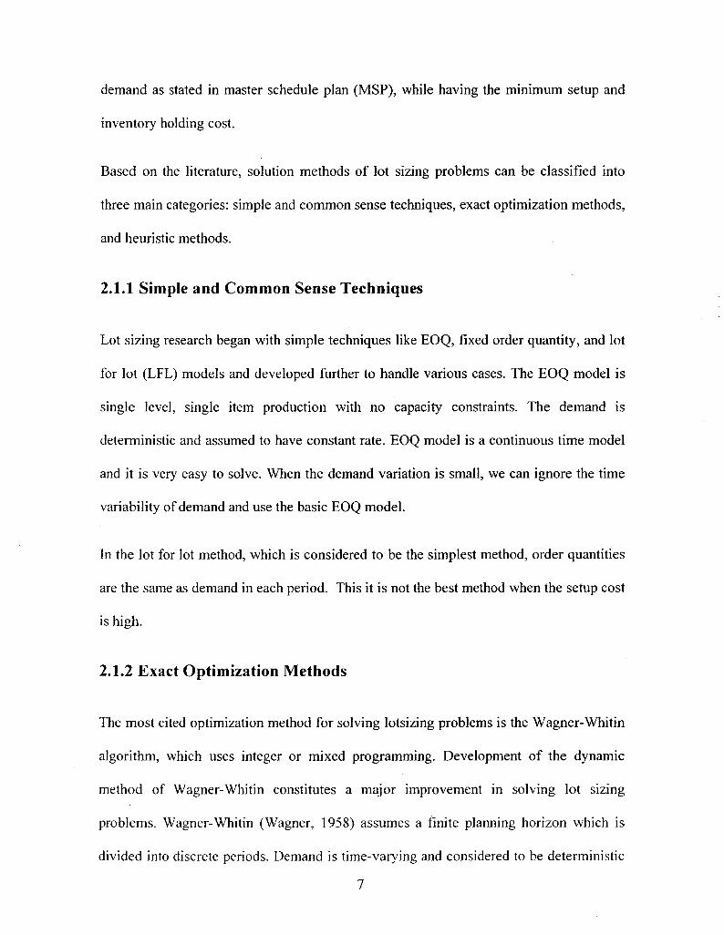
2.1.2.2 Mathematical Model
The single item capacitated lot sizing problem (CLSP) can be formulated as follows:
8
(2-1) Minimize TRC = £ AY; + I fh 7 = 1
ST.
Ij = / , + Qj - DJ
j = 1,..., t
7 y > 0
JO = {o,i}
Demand for each period (Dj) is given. The objective function minimizes the total relevant
cost of production (TRC) which is the summation of setup (A) and inventory holding
costs (h). In each period with production a set up cost will be incurred and this is modeled
by using a binary coefficient in the objective function. The first constraint is flow-balance
which shows the requirement in each period will produce at least one period before
needed period. As experiments showed, lot-sizing problems are NP-hard which is why
this field is dominated by heuristic techniques. The heuristic and meta-heuristic models
will be discussed in the next sections.
2.1.3 Heuristics
Heuristic methods are iterative procedures to solve a problem but do not grantee an
optimal solution. Heuristic methods are used for NP-hard problems when it is
computationally infeasible to find an optimal solution. The most common heuristic
approaches used to solve the lot sizing problem for dynamic demand are the Silver-Meal
(Meal, 1969), Least Unit Cost (LUC), and Part-Period Balance (PPB) methods.
9
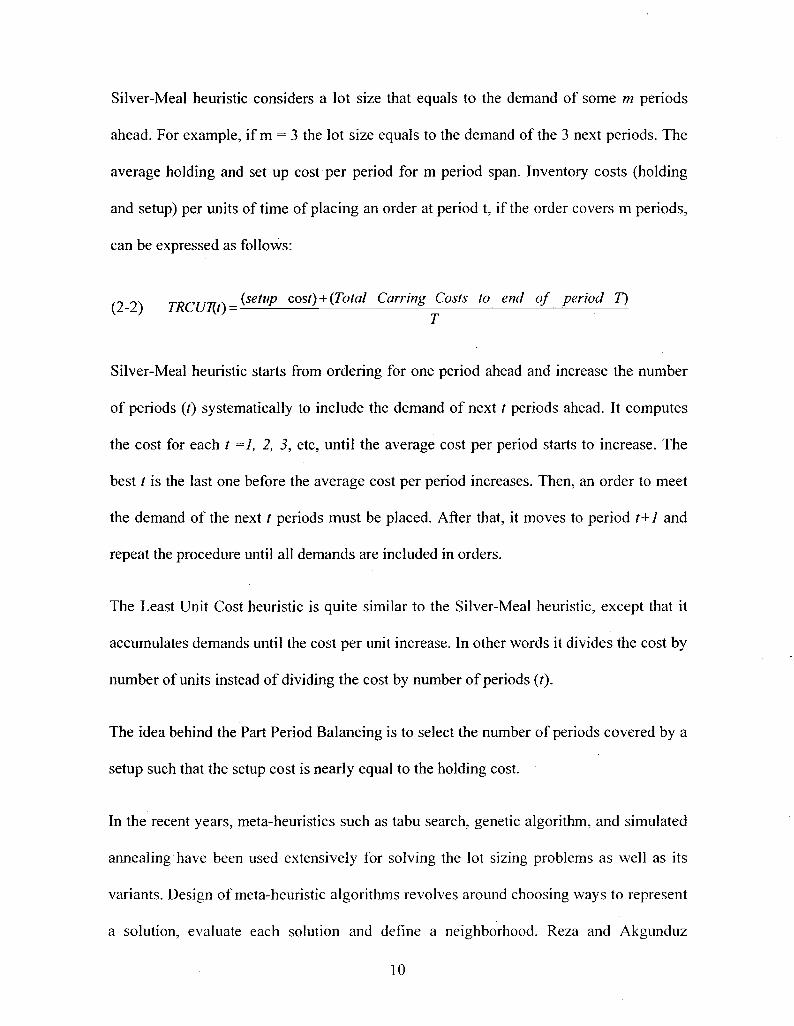
Silver-Meal heuristic considers a lot size that equals to the demand of some m periods
ahead. For example, if m = 3 the lot size equals to the demand of the 3 next periods. The
average holding and set up cost per period for m period span. Inventory costs (holding
and setup) per units of time of placing an order at period t, if the order covers m periods,
can be expressed as follows:
n 1 , T-omrn \ (settlP cost) + (Total Carring Costs to end of period T) (1-2.) lKLUl(t)-
Silver-Meal heuristic starts from ordering for one period ahead and increase the number
of periods (t) systematically to include the demand of next t periods ahead. It computes
the cost for each / =1, 2, 3, etc, until the average cost per period starts to increase. The
best t is the last one before the average cost per period increases. Then, an order to meet
the demand of the next t periods must be placed. After that, it moves to period t+1 and
repeat the procedure until all demands are included in orders.
The Least Unit Cost heuristic is quite similar to the Silver-Meal heuristic, except that it
accumulates demands until the cost per unit increase. In other words it divides the cost by
number of units instead of dividing the cost by number of periods (/).
The idea behind the Part Period Balancing is to select the number of periods covered by a
setup such that the setup cost is nearly equal to the holding cost.
In the recent years, meta-heuristics such as tabu search, genetic algorithm, and simulated
annealing have been used extensively for solving the lot sizing problems as well as its
variants. Design of meta-heuristic algorithms revolves around choosing ways to represent
a solution, evaluate each solution and define a neighborhood. Reza and Akgunduz
10
(2007), Ozdamar et al. (2002), Meyr (2000), and Sikora (1996), are a few examples of
the huge number of the existing literature on different variants of lot sizing. We will
discuss the design of their algorithms in more detail in the next sections and especially
those who use genetic algorithm in chapter 4.
2.1.4 General Characteristics of Lot Sizing Problems
There are many comprehensive reviews on the lot-sizing literature. Karimi et al. (2003)
classified the lot sizing problems into four categories based on the number of products
(single-item or multi-item) and the capacity (un-capacitated, capacitated). They also
introduced eight characteristic for lot sizing models. The following characteristics are to
be noted in any lot sizing models:
Planning horizon: Planning horizon can be discrete or continuous and it can also be
finite or infinite. For finite planning horizon with deterministic and time varying demand,
dynamic models like Wagner-Whitin are usually used.
Planning horizon can be categorized as either big bucket or small bucket. Big bucket
horizons are those where the time period is long enough to produce multi items, while for
small bucket problems the time period is so short that only one item can be produced in
each time period.
Production level: Production level can be either single or multi-level. Multi-level
production can further be categorized as serial, assembly, disassembly, and general. In a
single level production system, the final product with independent demand is directly
produced from raw or purchased materials, whereas in a multi-level production system, in
11
which items have the hierarchal relationship and output of one item is the input for
another one.
Number of products: There are two types of production with respect to the number of
products, namely single item and multi-item. Presence of sequence dependent setup times
and costs increase the complexity of planning for production of multi-item.
Demand for the end item: Demand can be deterministic (known in advance) or
probabilistic (not known exactly). It can be static (i.e. it will not change over time), or
time varying and dynamic.
Setup: Setup can be simple (independent of scheduling decisions) or complex. Complex
setups can further be categorized as setup with carry over, sequence dependent, and
family or major setup.
Deterioration of items: For items which can deteriorate, another constraint would
restrict the inventory holding time and add to complexity of the problem.
Inventory shortage: Backlogging and lost sales are two inventory characteristics which
can be allowed or not. Backlogging means that the demand of a period can be satisfied in
future.
2.2 Scheduling (Sequencing and Lot-Streaming)
A production setting, in which «-job should proceed in sequence of m machines or stages
and all the jobs are processed in the same sequence, is called a flowshop. Processing
times of different jobs on different machines may vary. All jobs are assumed to be
12
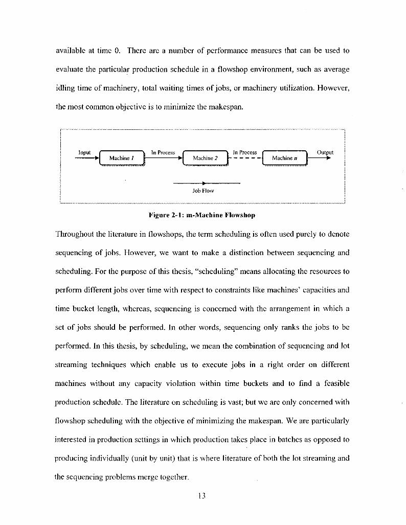
available at time 0. There are a number of performance measures that can be used to
evaluate the particular production schedule in a flowshop environment, such as average
idling time of machinery, total waiting times of jobs, or machinery utilization. However,
the most common objective is to minimize the makespan.
Input Machine /
In Process Machine 2
In Process ( Machine n
Output •
Job Flow
Figure 2-1: m-Machine Flowshop
Throughout the literature in flowshops, the term scheduling is often used purely to denote
sequencing of jobs. However, we want to make a distinction between sequencing and
scheduling. For the purpose of this thesis, "scheduling" means allocating the resources to
perform different jobs over time with respect to constraints like machines' capacities and
time bucket length, whereas, sequencing is concerned with the arrangement in which a
set of jobs should be performed. In other words, sequencing only ranks the jobs to be
performed. In this thesis, by scheduling, we mean the combination of sequencing and lot
streaming techniques which enable us to execute jobs in a right order on different
machines without any capacity violation within time buckets and to find a feasible
production schedule. The literature on scheduling is vast; but we are only concerned with
flowshop scheduling with the objective of minimizing the makespan. We are particularly
interested in production settings in which production takes place in batches as opposed to
producing individually (unit by unit) that is where literature of both the lot streaming and
the sequencing problems merge together.
We follow the three-field classes of scheduling problems introduced by Graham et al.
(1979). We use Fm/STsitt/Cmax to denote the problem studied in this thesis. In this
classification problems can be specified in terms of the three-field classification a /p / y
where a specifies the production environment, p specifies the job characteristics, and y
describes the objective function.
Fm represents flowshops with m-machines, in the second field, "STSj, t," sequence
independent setup times for sublots, and "Cmax " represents the performance measure of
minimization of makespan. In the rest of this section, the important notions and
definitions will first be discussed and then the literature of lot streaming and sequencing
will be presented briefly.
Sequencing research starts with the very early works of Johnson's 1954 paper on two
machine flow-shop scheduling (Johnson, 1954). Reiter (1966) introduced the concept of
lot streaming.
Lot streaming is the process of splitting a job or a lot to allow overlapping between
successive operations in a multi-stage production system. This usually results in a shorter
makespan. In the context of multi-product lot streaming in addition to the sublot sizes and
the number sublots the production sequence of items is another decision variable.
Chang and Chiu (2005) classified lot streaming problems into four categories based on
number of products (single or multiple) and the performance measurements (time-related
and cost-related). They described lot streaming problems with three main dimensions,
namely system configuration, sub-lot-related feature, and performance measurement.
14
They also introduced seven sub-dimensions which has several levels as shown in
appendix 2.
2.2.1 Notions and Classifications
In the rest of this section, we introduce the necessary definitions and classifications.
1. In an m-machine flowshop, a schedule is called permutation if the job sequence
stays the same on all the machines or stages. Otherwise, it is a non-permutation
schedule.
2. Sequencing problem in a flowshop can be categorized further to those with
independent setup and those with sequence dependent setup times.
3. A setup is attached if it cannot be started before the production lot or sublot
becomes available on the machine. If it can starts before availability of sublot a
setup is detached.
4. Lot or sublot sizes can be consistent, equal, or variable. Consistent batches have
the same size over the different stages or machines. If all the sublots' sizes are
equal it would be called equal sublots otherwise, it would be called variable sublot
size.
5. Idling can be allowed or not. Machines can be idle between sublots if intermittent
idling is allowed. Non-idling means that sublots should be processed one after the
other on a particular machine or stage.
6. Setup, production, and transportation are the three types of activities that involve
a series of operation.
15
7. Sublot size can be a real number or an integer (discrete or continuous). For
discrete sublots, the number of item in a sublot has to be integer number. While,
for continuous sublots size there is no restriction on the sublot size. For example,
in chemical industries sublots take continuous numbers.
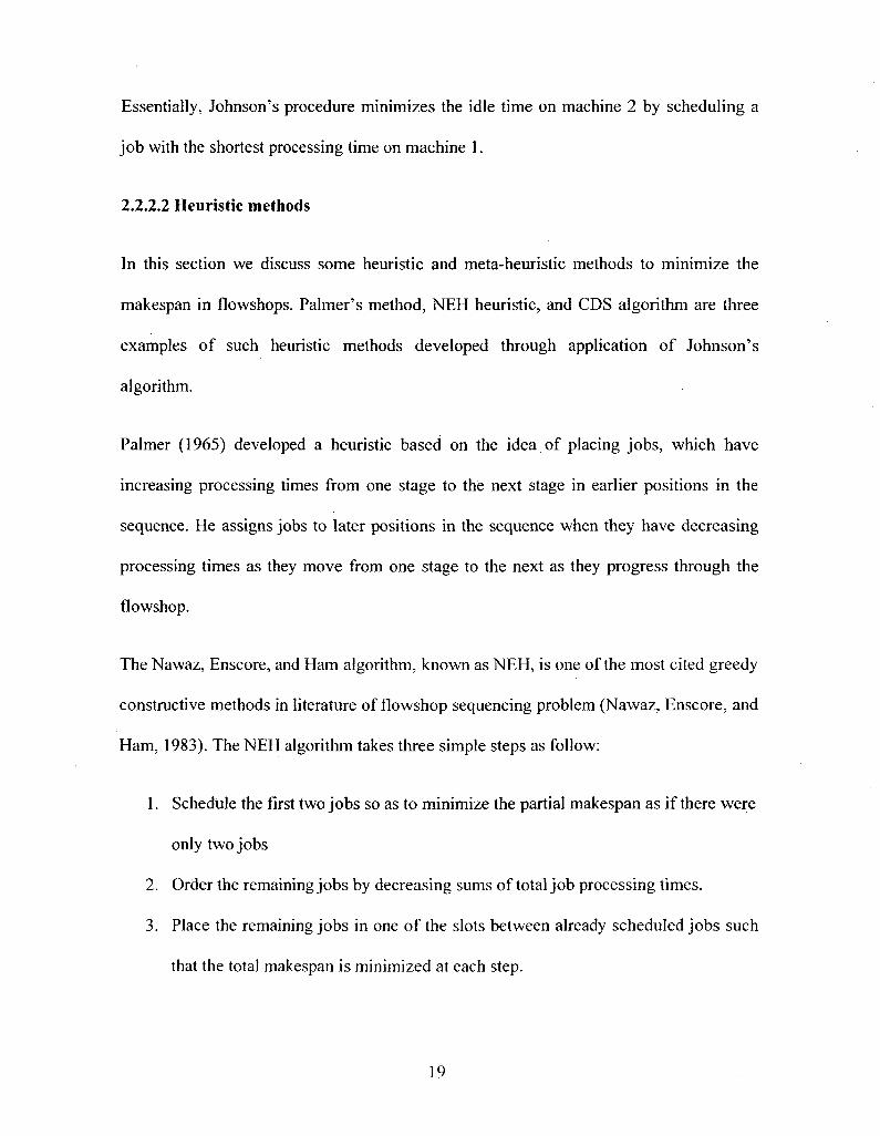
In multi-product setting, if intermingling sublots (preemptions) is allowed, the sequence
of sublots of a given product may be interrupted by sublots of another product. For non-
intermingling sublots, no interruption in the sequence of sublots of a product is allowed
(Defersha and Chen 2008). In other words, production of a particular product on one
machine or stage can be started once the last sublot of the previous product is finished.
Figure 2-2, in the next page, shows the benefits of lot streaming in reducing the
makespan (Chang and Chiu, 2005).
16
M ]
M2
M3
i:*!!
;..S()
1 JO
| Without Splitting!
,.{!>
12!)
i;>»>
t i i n c
M l
M2
M3
<)<> w)
'111
w l M )
f>0
*.""
<>0
S » t
Two Equal Sublots
t i m e
M l
M3
-10 -»<> •H>
~ j t >
( • t o -1(1
-SO
-It)
-SO
*SU
-1(1
^Mt
(Three Equal Sublots!
t i m e
M 1
M2
M3
"0 5tt
Vi(>
7{i 5is
71 >
M M
M»
<•«)
| Consistent Subk
11 rnc
Figure 2-2: Gantt Charts of Different Sublot Sizes
17
2.2.2 Common Solution Methods
There are two main approaches to solve flowshop scheduling problems namely, the exact
and heuristic approaches. There are a huge number of studies on both the exact and
heuristic solution procedures developed to solve the scheduling problems in flowshops.
The exact algorithms are capable of determining the optimal solutions. However,
heuristics approaches are also very prominent in t2he literature since such problems are
proven to be NP-complete.
2.2.2.1 Exact techniques
Sequencing research starts with the very early works of Johnson's 1954 paper on two
machine flow-shop scheduling (Johnson, 1954). Johnson developed a procedure that
minimized the makespan for jobs on two machines. For a two-machine setting, Johnson's
solution is proven be an optimal solution and it can be extended to a three-machine
flowshop problem as well. The Johnson's algorithm also known as Johnson rule is as
follows:
1. Determine the shortest processing time among all jobs yet to be sequenced on
machine 1 and 2.
2. Schedule the job associated with the shortest processing time first in the sequence,
if it occurs on the first machine.
3. Schedule the job associated with the shortest processing time last in the sequence,
if it occurs on the second machine.
4. Continue until all the remaining jobs are scheduled.
18
Essentially, Johnson's procedure minimizes the idle time on machine 2 by scheduling a
job with the shortest processing time on machine 1.
2.2.2.2 Heuristic methods
In this section we discuss some heuristic and meta-heuristic methods to minimize the
makespan in flowshops. Palmer's method, NEH heuristic, and CDS algorithm are three
examples of such heuristic methods developed through application of Johnson's
algorithm.
Palmer (1965) developed a heuristic based on the idea of placing jobs, which have
increasing processing times from one stage to the next stage in earlier positions in the
sequence. He assigns jobs to later positions in the sequence when they have decreasing
processing times as they move from one stage to the next as they progress through the
flowshop.
The Nawaz, Enscore, and Ham algorithm, known as NEH, is one of the most cited greedy
constructive methods in literature of flowshop sequencing problem (Nawaz, Enscore, and
Ham, 1983). The NEH algorithm takes three simple steps as follow:
1. Schedule the first two jobs so as to minimize the partial makespan as if there were
only two jobs
2. Order the remaining jobs by decreasing sums of total job processing times.
3. Place the remaining jobs in one of the slots between already scheduled jobs such
that the total makespan is minimized at each step.
19
Campbell et al. (1970) developed an algorithm; known as the CDS algorithm which uses
Johnson's rules. The algorithm breaks the m-machine problem into several two-machine
problems, then each of two-machine problems is solved using Johnson's two-machine
algorithm.
Sriskandarajah and Wagneur (1999) considered the problem of minimizing makespan in
two-machine and no-wait flow shop with multiple products. Their objective is to
determine sublot sizes and sequence the jobs simultaneously. They develop a heuristic
procedure to solve sequencing and lot streaming of multiple products. Computational
results are shown to be close to the optimal. Later, Kumar et al. (2000) extends the two-
machine model of Sriskandarajah and Wagneur to m-machines lot streaming problem.
Lot streaming for multiple products in a multi-stage flow shop with equal sublots and no
intermingling is discussed by Kalir and Sarin (2001). Their objective was to minimize the
makespan by finding the right sequence for jobs. They developed a heuristic procedure
for the lot-streaming and sequencing problems. They used an example to show the
importance of sequencing in lot streaming problems.
Hall et al. (2003) studied the problem of minimizing the makespan in flowshop with lot
streaming. Their model required the sublots to be processed consecutively on each
machine. Setups occur only between sublots of different families. Setups are either all
detached or all attached. They showed that this problem can be formulated as a general
traveling salesman problem. Furthermore, they proposed a heuristic for multiple
products, no wait processing and lot streaming flowshop problem.
20
Biskup and Feldmann (2006) introduced the very first MIP formulation for single item in
multi-stage production settings with variable sublots sizes. They showed that significant
makespan reduction can be achieved by using variable sublot sizes. Defersha and Chen
(2008) extended the single item lot streaming model of Biskup and Feldmann (2006) to
multiple products and proposed a genetic algorithm. Their model is outstanding in
tackling the sequencing and splitting problem simultaneously. Their model also
outperforms that of earlier approaches because their model of variable sublots also allows
intermingling of sublots.
2.3 Integrated Lot-Sizing and Scheduling
In the most of the literature of production planning, lot sizing and scheduling problems
are solved independently and, for the sake of simplifying the problem, the
interdependencies of lot size, sequence, and capacity usage are ignored. The problem
discussed here is the lot sizing and scheduling of ^-product in a flowshop consist of m
machines with the objective of minimizing total inventory holding cost and setup costs.
Demand has a deterministic and dynamic pattern over a finite planning horizon and must
be met without back-logging. Production takes place in lots. In this condition, lot sizing
and scheduling of jobs should be done simultaneously because we encounter sequence
dependent setup times and production which takes place in lots.
First, in presence of sequence dependent setup times, the limited capacity available for
production may be reduced by changeovers causing sequence-dependent setup times.
Thus, lot sizing and capacity usage depends on both the sequence and the size of the
sublots.
21
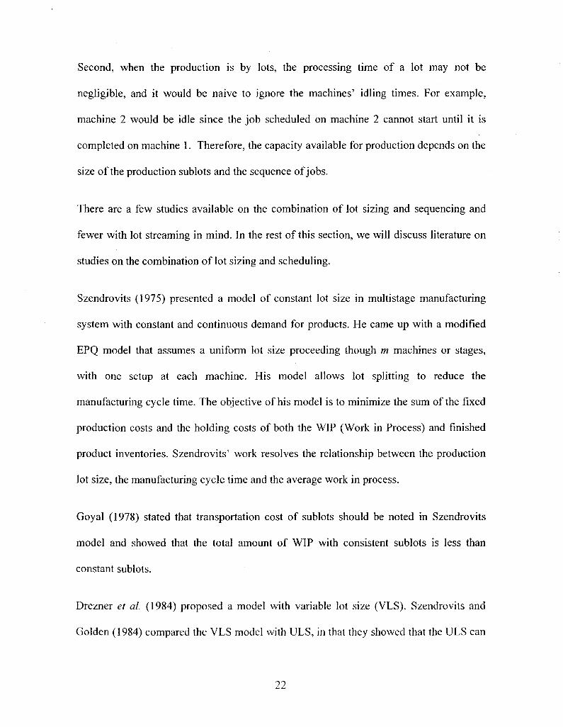
Second, when the production is by lots, the processing time of a lot may not be
negligible, and it would be naive to ignore the machines' idling times. For example,
machine 2 would be idle since the job scheduled on machine 2 cannot start until it is
completed on machine 1. Therefore, the capacity available for production depends on the
size of the production sublots and the sequence of jobs.
There are a few studies available on the combination of lot sizing and sequencing and
fewer with lot streaming in mind. In the rest of this section, we will discuss literature on
studies on the combination of lot sizing and scheduling.
Szendrovits (1975) presented a model of constant lot size in multistage manufacturing
system with constant and continuous demand for products. He came up with a modified
EPQ model that assumes a uniform lot size proceeding though m machines or stages,
with one setup at each machine. His model allows lot splitting to reduce the
manufacturing cycle time. The objective of his model is to minimize the sum of the fixed
production costs and the holding costs of both the WIP (Work in Process) and finished
product inventories. Szendrovits' work resolves the relationship between the production
lot size, the manufacturing cycle time and the average work in process.
Goyal (1978) stated that transportation cost of sublots should be noted in Szendrovits
model and showed that the total amount of WIP with consistent sublots is less than
constant sublots.
Drezner et al. (1984) proposed a model with variable lot size (VLS). Szendrovits and
Golden (1984) compared the VLS model with ULS, in that they showed that the ULS can
22
give a better result in minimizing the cost in some situations but it depends on the sublot
transportation cost.
Smith and Ritzman (1988) presented a mixed integer programming formulation for lot
sizing problem considering the sequencing problem. Their formulation considers
sequence dependent set-up times and capacity constraints. However, the MIP formulation
is not always able to solve real size (large) problems.
Sikora et al. (1995) studied the problem of flowshops with finite scheduling horizon with
objective of minimizing the makespan and inventory holding cost. The flowshop they
discused has the following characteristics:
• Sequence dependent setup times,
• Limited intermediate buffer space,
• capacity constraints,
• In addition jobs are assigned with due dates that have to be met.
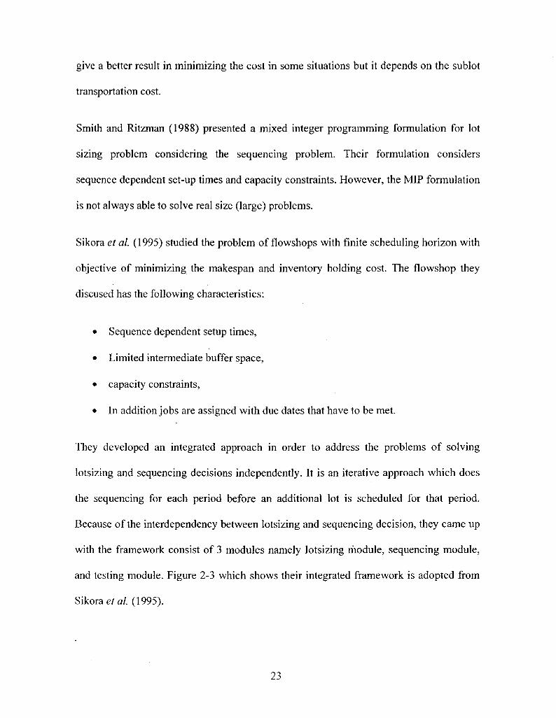
They developed an integrated approach in order to address the problems of solving
lotsizing and sequencing decisions independently. It is an iterative approach which does
the sequencing for each period before an additional lot is scheduled for that period.
Because of the interdependency between lotsizing and sequencing decision, they came up
with the framework consist of 3 modules namely lotsizing module, sequencing module,
and testing module. Figure 2-3 which shows their integrated framework is adopted from
Sikora et al. (1995).
23
Daily Demand"
Lot Sizing
Available Capacity
Setups
Sequence
Lot Sizing
J
Lot Sizing 1
Makespan
Manufacturing Environment
Daily Schedule
Figure 2-3: The Integrated Framework of Scheduling System
In each iteration, the lot sizing module calls the sequencing module to find the optimal
sequences which minimize the makespan. Then, the testing module calculates the
makespan and residual capacity on the bottleneck machine for the given lot size and
sequence and information will be returned to lot sizing module before any additional lot
be scheduled in the period.
The lot sizing module uses a modified version of Silver Meal heuristic that allows lot
splitting in order to increase the capacity usage. It calculates b, which is the fraction of
the next period's (7/ + 1) demand that can be produced in the current period without
violating the capacity constraints. Then, it quantifies the TRCUT (total relevant cost per
unit of time) based on this fraction (b), using the following formulation:
24
. . ,, remaining capacit (2-3) 9 =mirKl,—
Wa </;+i)
A+h^id-T'^+h.D^b, (2-4) TRCUT(Ti+l,bi) = ^
T.-T
Where:
kj Required capacity for producing one unit of product i
D^ Demand of item / in period d
Aj Setup cost for item /
hi Inventory holding cost for item /
T* The current period
Tj The number of periods ahead in planning horizon
The sequencing module uses an improved version of palmer heuristic and the pair-wise
exchanged which incorporates the sequence dependent set up times and the limited buffer
capacities.
Sikora (1996) developed a genetic algorithm for integrating lot sizing and sequencing
problems in a flowshops with all the characteristics of the integrated approach described
previously by Sikora et al. (1995). In their proposed genetic algorithm, each possible
solution is represented by a string of paired values for each period in the time horizon.
The first number of any pair indicates the type of job and the second number indicates the
number of units of that job type that have to be produced (lot-size). The order of the pairs
indicates the sequence of jobs.
25
In order to enable the genetic algorithm to manipulate both data of lot sizing and
sequencing, they use separate crossover and mutation operators. Their GA uses
tournament selection mechanism. The feasibility of the initial population is assured by
scheduling the lot size s equal to demand in that period. Finally, experiments showed that
their genetic algorithm outperforms both the integrated and sequential approaches.
Ozdamar and Birbil (1998) developed a hybrid heuristic consisting of meta-heuristics
such as simulated annealing (SA), tabu search (TS) and genetic algorithms (GA) for
solving the capacitated lot sizing and loading problem (CLSLP). They define the CLSLP
problem as determining the lot size of product families and loading them on parallel
machines.
Meyr (2000) introduced another model for solving lotsizing and scheduling problems
simultaneously in a capacitated flowshop with sequence dependent setup times. Their
model combines a simulated annealing heuristic with the mixed integer model to solve
the problem by fixing the binary variable of setup sequence and solve the sub-problems
by heuristic. Then, they discuss that solving each of sub-problems to optimality is too
time consuming. They develop a mathematical solution which remodels the problem as a
dual network flow problem. The computational tests prove that their procedure is
efficient.
Ramasesh et al. (2000) proposed an EOQ model for a single item in multistage when lot
streaming is applied. They develop a total cost function consisting of the inventory
holding costs, setup cost, transportation cost, and also WIP carrying cost, and then they
discuss a procedure to find the optimal production lot size that minimizes the total cost.
26
Their contribution is twofold; they capture more accurately the components of the
manufacturing lead time that are encountered in a multistage production environment,
and they use the lot streaming in a multistage system MRP.
Hoque and Goyal (2003) claimed that Ramasesh model (Ramasesh, 2000) is not only a
special case of the model of Hoque and Kingsman (1995) but also is not able to find the
minimum cost. They solved two examples, which one of them had been solved by
Ramasesh (2000) and the results showed a significant reduction in cost.
2.4 Lead Time
Lead times in MRP systems represent the planned amount of time allowed for orders to
flow through the manufacturing system (Kanet, 1986). Lead time is important because it
can affect every component of an MRP-based manufacturing and it is related to capacity
planning. Lead time structure or the way that lead times are estimated is under
management's complete control, and can change the pattern of planned order releases as
well as flow time and the amount of inventory.
Lead-time determination can change the pattern of planned order releases in an MRP
system. Moreover, by changing the order release pattern the bottleneck facilities would
change. This results in unpredictable lead times and capacity. Kanet (1986) compared
different lead time structures but did not find any evidence to show which structure is
better. In other studies, the results show that the commonly used structure (processing
time + setup + waiting time) does not have a better result, especially when the criterion is
tardiness (Kanet, 1981).
27
Many researchers believe that holding planned lead times down will decrease the
inventory and eventually yield benefits. They argue that there is a vicious circle of lead
time, which means that an increase in lead time encourages shop personnel to ignore
deadlines. As a result more increases in lead time are required. Furthermore, it becomes
increasingly difficult to plan the MPS because as lead times increase forecasts become
more inaccurate. However, Kanet (1986) categorizes the inventory and creates an
example that shows lowering the lead times does not always result in reduction in
inventory levels. He also came up with a simple and very intuitive rule:
"If storeroom inventory contains less early inventory than delayed
inventory then lead times should be increased. If storeroom inventory
contains earlier inventory than delayed inventory, then lead times
should be reduced."
From the above mentioned studies we conclude that we cannot ignore the interaction of
lead time, lot size, and capacity usage. Since different lot size, sublot size, and sequence
has direct impact in on lead time we should find way to find the actual lead time while we
are deciding on lot size.
28
CHAPTER 3
MATEMATICAL FORMULATION
As mentioned in previous chapters, our objective is to decide the sequence of the
production and the sublot sizes while solving the lot sizing problem. This will result in
better scheduling, since the sublot sizes and the sequence of production are known, we
will know the idling times of machines and be able to fill them with jobs, and the orders
released to shop floor will be definitely feasible.
In this chapter, a mixed integer linear programming (MILP) formulation is presented. It
enables us to simultaneously find the optimal lot sizes, as well as the corresponding
sublot sizes and sequences. This model takes the demand as an input and gives the
optimal lot size, sublot size, and the sequence of production as an output. With this
model, small size problems can be solved within a reasonable time. This model also
calculates the makespan, in order to ensure that makespan is less than the available time
in each period. Moreover, the lead time is explicitly computed in the model.
3.1 Assumptions and Limitations
To find the best production batch size will make a number of simplifying assumptions:
29
1) The demand is time varying, known and deterministic
2) The inventory holding cost is only applicable to the inventory that is carried over
from one period to the next
3) Production must be completed at the end of each period to meet the demand,
4) Jobs should be processed in sequence M machines or stages,
5) Each production order (lot size) consists of Q identical items which would be
divided into sublots
6) Items become available for processing at the next machine whenever the
processing of the whole sublot has been finished on the previous machine
7) The entire production lot is produced with a single setup on each machine and
transferred to the next machine in one or more sublots
8) The cost factors do not change with time. In other words, inflation is negligible
9) No shortage is allowed
The proposed linear programming formulation to solve the lot sizing problem with the
above assumptions is a combination of the conventional model of lot sizing commonly
abbreviated as CLSP (Karimi, Fatemi, and Wilson, 2003) and lot splitting with variable
lot size quite similar to (Biskup and Feldmann, 2006).
3.2 Notations
Let the parameters be:
Djt Demand for the Product j in period /
St m Setup time of machine m for the Product j
Sc/ Setup cost for the Product /
30
r Processing time for one unit of the Product / on machine m
/ Fixed minimum lead time (not include an estimate of delay due to
machines idling times or capacity constraints)
h Inventory holding cost
Capml Available time on machine m in period t
TBr Available units of time (time bucket) in period /
S Number of sublots
s Indices for sublots, s = \,...,S
N Number of products
j Indices for products, 7 = 1,...,N
M Number of machines
m Index for the machines, m = 1,...,M
A Sufficiently large number
Let the Decision variables be:
Lj, Lot Size (quantity to be produced from product j in each period/)
U j s, Size of the sublot s of the Product j in period /
/ ., Ending inventory of the Product j in period /
Xj k, Binary variable, which takes the value 1 if the Product j on machine m
has started before the Product k , takes 0 otherwise.
Yj, Binary variable, which takes value 1 if production of the Product J take
place in period t
31
b sml Starting time of the sublot s of product j on machine m in period t
Pjsml Processing time of sublot 5 of product j on machine m in period/
3.3 Mathematical Model
(3-D MIN = x z /,., * *+z i > , * Y.,.> 7 = 1 / = 1 ,/ = l 1 = 1
(3-2) / ; ,_, + Lji_r - ihi = DJI j = ],..., N / = /%..., T
(3-3) ^{L^r^+Stj^Yj^KCap^ t = \,...,T m = ],...,M y=i
(3-4) bjSMj + PJiSMj < TB, j = 1,..., N t = I,..., T
(3-5) LJI-A*YJI < 0 j = \,...,N t = ],...,T
(3-6) ! > , , , , = ^ , J = l-,N / = !,...,r
(3-7) Pj,s,m.,=Uj,s,,*rj,m j = 1,...,N t = ],...,T m = h...,M s = \,...,S
(3-8) 6,,s,m,, + PJM + Stkm *Ykl < bksm, + (1 - X j k , ) A
j,k = ],..., N j<k s = ],..., S m = ],..., M t = ],...,T
(3-9) bksm_, + Pk^, + Stjm * Yhl < bJsml + xJkl * A
j , k = ],..., N j <k s = ],..., S t = 1,..., T m = 1,..., M
(3-10) bJ]ni,>bJlm_ll+P/Xm_]l+Sthm j = ],...,N t = ],...,T m = 2,...,M
(3-11) bJAXl>St„ j = \,...,N t=l,...,T
(3-12) ^ „ , , > ^ _ L „ , , + ^ . . ( . , . „ , ,
32
j = 1,..., N , t = 1,..., T, m = 1,..., M s = 2,..., S
(3-13) y,,, > * M , j,k = },...,N t = \,...j
(3-14) / 7 „ ^ / , ^ , , ^ m „ / > / j m , >0 y = l,...,iV / = l,...,r » = 1 M i = l 5
(3-15)7,,, = 0,or 1 J = l-,N t = ],...,T
(3-16)Xj.k..=°>or} j,k = ],...,N j<k / = ],..,r
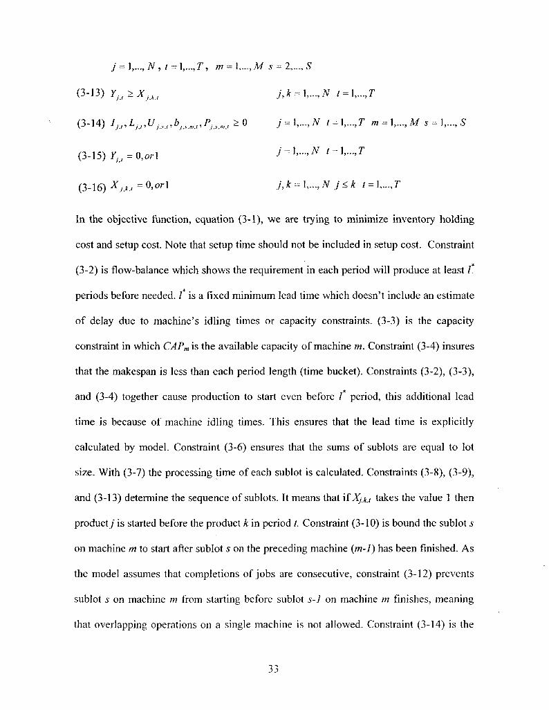
In the objective function, equation (3-1), we are trying to minimize inventory holding
cost and setup cost. Note that setup time should not be included in setup cost. Constraint
(3-2) is flow-balance which shows the requirement in each period will produce at least /
periods before needed. / is a fixed minimum lead time which doesn't include an estimate
of delay due to machine's idling times or capacity constraints. (3-3) is the capacity
constraint in which CAPm\s the available capacity of machine m. Constraint (3-4) insures
that the makespan is less than each period length (time bucket). Constraints (3-2), (3-3),
and (3-4) together cause production to start even before / period, this additional lead
time is because of machine idling times. This ensures that the lead time is explicitly
calculated by model. Constraint (3-6) ensures that the sums of sublots are equal to lot
size. With (3-7) the processing time of each sublot is calculated. Constraints (3-8), (3-9),
and (3-13) determine the sequence of sublots. It means that \iXjxt takes the value 1 then
product/ is started before the product k in period /. Constraint (3-10) is bound the sublot s
on machine m to start after sublot s on the preceding machine {m-1) has been finished. As
the model assumes that completions of jobs are consecutive, constraint (3-12) prevents
sublot 5 on machine m from starting before sublot s-l on machine m finishes, meaning
that overlapping operations on a single machine is not allowed. Constraint (3-14) is the
33
non negativity constraint. Constraints (3-15) and (3-16) restricts X and Y variables to
binary form.
3.4 Computational Experiments
3.4.1 A Numerical Example
Through the following example we will show how simultaneous lot streaming can affect
lot sizing process and how it ensures the feasibility of the orders released to shop floor
and reduces scheduling nervousness. Assuming a production setting of a single product in
which each lot of Q units must proceed in sequence of 4 machines with associated unit
processing time of 8, 4, 8, and 4 respectively on each machine. The availabilities on each
machine are 160, 80, 160, and 70 units of time respectively. Each lot may be divided into
4 sublots, though the entire production lot is produced with a single setup of $100 on
each machine. The inventory holding cost of $10 is only applicable to inventory that is
carried over from one period to the next period. For each period (Month) we assumed 200
working units of time. Demand over the planned horizon, order released by conventional
lot sizing models, and order released by our model are as shown in table 3-1.
Month Demand Order released by conventional model Order released by our model
Jan 10 5 6
Feb 5 14 16
Mar 10 17 16
Apr 20 17 16
May 15 17 16
Jun 20 0 0
Table 3-1: Demand and Order released in Planning Horizon
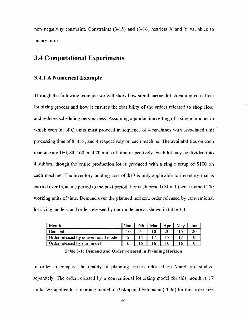
In order to compare the quality of planning, orders released on March are studied
separately. The order released by a conventional lot sizing model for this month is 17
units. We applied lot streaming model of Biskup and Feldmann (2006) for this order size
34
(Q=17), and as shown in figure 3-1 (a), the optimal sublot size would be 5, 5, 5, and 2
with the makespan of 208 hours. This would be an infeasible order because there are only
200 available working hours per month. In other words, the conventional lot sizing
model assigned a load that exceeds the shop floor's available time by 8 hours during the
months of March, April, and May. Figure 3-1 (b) illustrates order released by our model
(Q=16) with four sublots of size 4 and the makespan of 200 hours. Given the net required
values are the same as ones been proposed by conventional lotsizing models, our model
is able to resolve the infeasibility without changing the Master Schedule Plan (MSP).
M l
Mi
M i
M l
&;*S | &.-eS 1 , „ 5 1 1 .1
| |
c 1 - 1
S««$ |
c
l - l hi &aS | !*;:«* | j V>i*2 |
2R3
- 1 l ~ l l - I ' l ao 2c JO y t so a ; 3o sc- sc iso n e u c iso i-*c i>o ; t o i ;o i sc ist> ?oc 2i5 ^20
b.
M l
M2
Mi
M i l
1
1
4
|
1
1 1 «
1 1 - 1 1
r7" i
i
i i
i
Z3
1 • 1 1 * 1
X*a
1 - 1 - 1 LiJ 3 SO '.'P JO *-•> SO ICO 111? 12C HO 1*0 1>C IttV l?C 3ST 130 ?0O 2S« 2.:.'
Figure 3-1: Gantt Chart of Production in Month of March
3.4.2 Analytical Examples
For testing, this mathematical model was coded for Lingo 10.0 (see the appendix 3). We
also generated two sets of random problems with different number of machines, products.
and number of planning periods. Then, we solved each problem twice with different time
bucket length. The required parameters of problems are as follows:
• Number of periods in the planning horizon is 6 or 12.
• The number of products N:{ 3,7,9,10,12,14,15,17}
• The number of machines M: {4, 5, 6, 7, 8, 10, 12,15}
• Maximum number of sublots allowed is 4
• Inventory holding costs and setup costs are considered constant and equal to 10,
100 respectively.
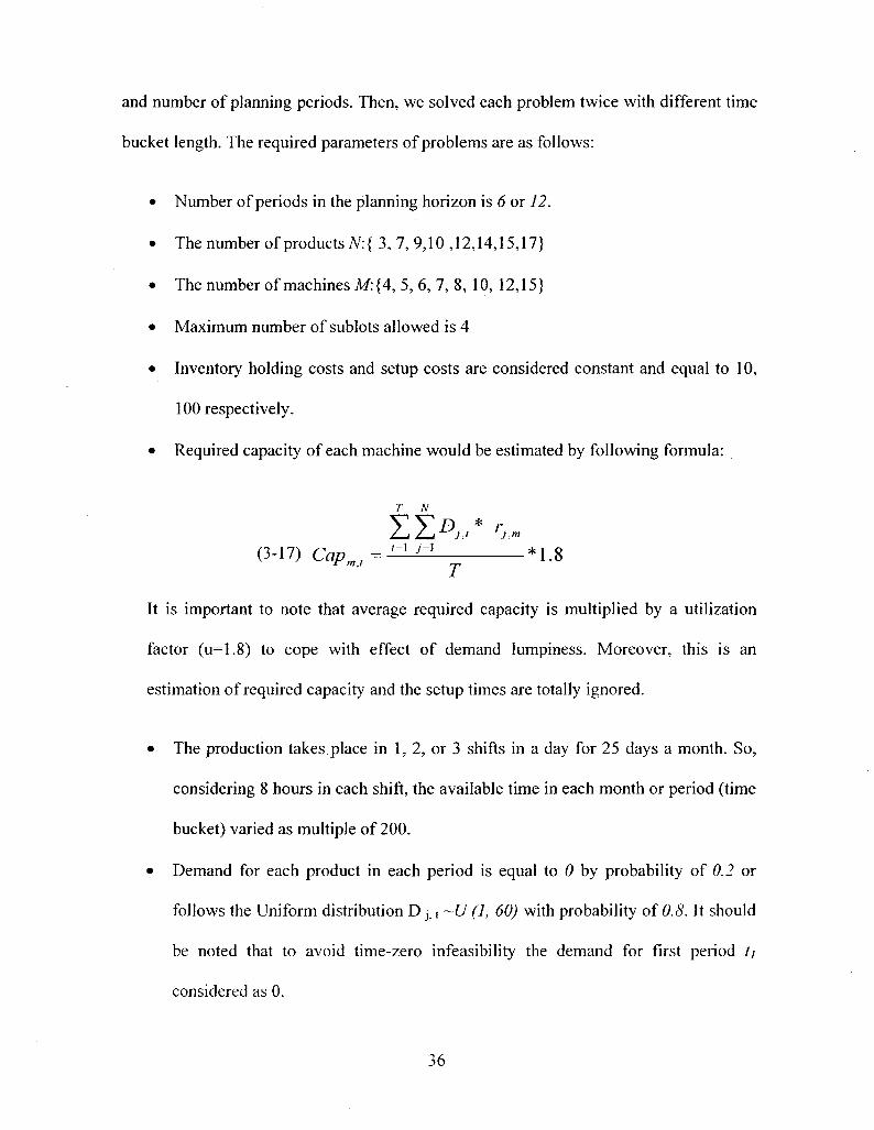
• Required capacity of each machine would be estimated by following formula:
T N
(3-17) CapmJ=SU^—. *1.8
It is important to note that average required capacity is multiplied by a utilization
factor (u=1.8) to cope with effect of demand lumpiness. Moreover, this is an
estimation of required capacity and the setup times are totally ignored.
• The production takes place in 1, 2, or 3 shifts in a day for 25 days a month. So,
considering 8 hours in each shift, the available time in each month or period (time
bucket) varied as multiple of 200.
• Demand for each product in each period is equal to 0 by probability of 0.2 or
follows the Uniform distribution D j. t ~U (1, 60) with probability of 0.8. It should
be noted that to avoid time-zero infeasibility the demand for first period tj
considered as 0.
36
• Processing times of each units of product on each machine m follows the Uniform
distribution r7 m ~U (1, 5).
• Setup times follow Uniform distribution St j : m ~U (5, 20).
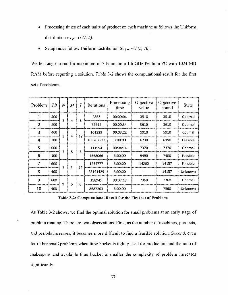
We let Lingo to run for maximum of 3 hours on a 1.6 GHz Pentium PC with 1024 MB
RAM before reporting a solution. Table 3-2 shows the computational result for the first
set of problems.
Problem
1
2
3
4
5
6
7
8
9
10
TB
400
200
400
200
600
400
600
400
600
400
N
3
3
7
7
9
M
4
4
5
5
6
T
6
12
6
12
6
Iterations
2853
72212
101239
108702522
111594
4668066
1234777
28141429
158945
8687203
Processing time
00:00:04
00:00:54
00:03:22
3:00:00
00:04:14
3:00:00
3:00:00
3:00:00
00:07:18
3:00:00
Objective value
3510
3610
5910
6230
7370
9490
14200
-
7360
"
Objective bound
3510
3610
5910
6190
7370
7400
14157
14157
7360
7360
State
Optimal
Optimal
optimal
Feasible
Optimal
Feasible
Feasible
Unknown
Optimal
Unknown
Table 3-2: Computational Result for the First set of Problems
As Table 3-2 shows, we find the optimal solution for small problems at an early stage of
problem running. There are two observations. First, as the number of machines, products,
and periods increases, it becomes more difficult to find a feasible solution. Second, even
for rather small problems when time bucket is tightly used for production and the ratio of
makespans and available time bucket is smaller the complexity of problem increases
significantly.
37
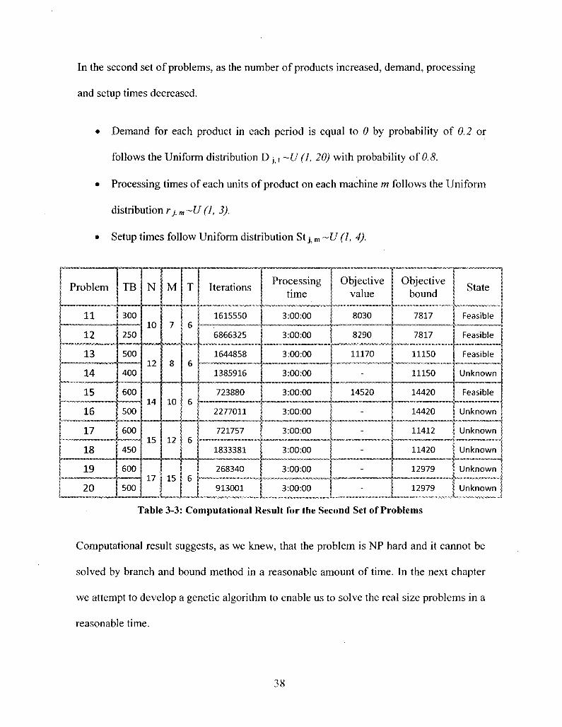
In the second set of problems, as the number of products increased, demand, processing
and setup times decreased.
• Demand for each product in each period is equal to 0 by probability of 0.2 or
follows the Uniform distribution D j . t ~U (1, 20) with probability of 0.8.
• Processing times of each units of product on each machine m follows the Uniform
distribution r7> m ~U (J, 3).
• Setup times follow Uniform distribution St j . m ~U (I, 4).
Problem
11
12
13
14
15
16
17
18
19
20
TB
300
250
500
400
600
500
600
450
600
500
N
10
12
14
15
17
M
7
8
10
12
15
T
6
6
6
6
6
Iterations
1615550
6866325
1644858
1385916
723880
2277011
721757
1833381
268340 [ ™ *""""•
913001
Processing time
3:00:00
3:00:00
3:00:00
3:00:00
3:00:00
3:00:00
3:00:00
3:00:00
3:00:00
3:00:00
Objective value
8030
8290
11170
-
14520
-
-
-
-
0^ j eCt i;e 1 State bound |
7817 j Feasible
7817 | Feasible
11150 I Feasible
11150 J Unknown
14420 Feasible
14420 1 Unknown
11412 J Unknown
| 11420 Unknown
8
12979 j Unknown
12979 Unknown
Table 3-3: Computational Result for the Second Set of Problems
Computational result suggests, as we knew, that the problem is NP hard and it cannot be
solved by branch and bound method in a reasonable amount of time. In the next chapter
we attempt to develop a genetic algorithm to enable us to solve the real size problems in a
reasonable time.
38
CHAPTER 4
GENETIC ALGORITHM
During the last decades we have seen a growing interest in heuristic algorithms which are
based on evolution and survival of the fittest, especially for global optimization problems
like lotsizing and other NP-hard problems. The best known algorithms of this kind
include genetic algorithms, Tabu Search, and Simulated Annealing, as well as some
hybrid algorithms which integrate various features of the above methods.
This chapter includes an introduction to genetic algorithms and a brief overview of the
important genetic algorithms used in lot sizing and scheduling problems in the literature.
Then we present the developed genetic algorithm.
4.1 Genetic Algorithms: An Overview
The Genetic Algorithm (GA), developed by Holland in 1975, is a one of the meta-
heuristic methods used to solve complex optimization problems. GA searches the
solution space randomly and do not guarantee an optimal solution. In practice, however,
along with advantages; such as flexibility and straightforwardness, the results are usually
extremely good. GA is an iterative heuristic search procedure following the principles of
39
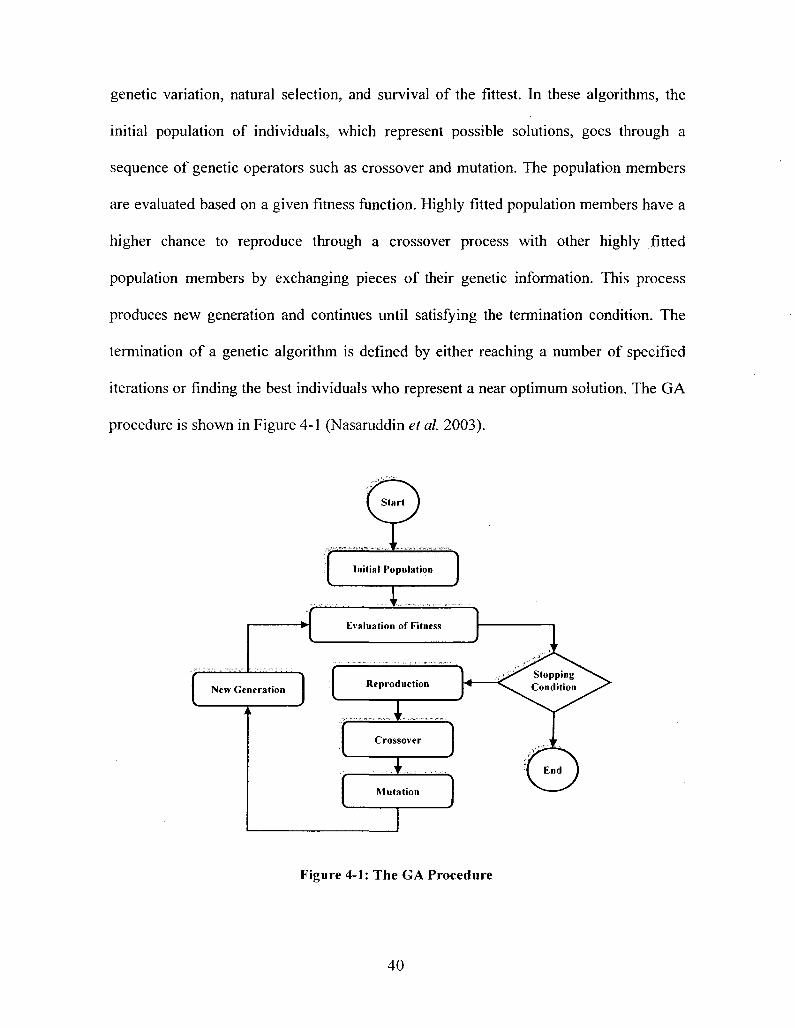
genetic variation, natural selection, and survival of the fittest. In these algorithms, the
initial population of individuals, which represent possible solutions, goes through a
sequence of genetic operators such as crossover and mutation. The population members
are evaluated based on a given fitness function. Highly fitted population members have a
higher chance to reproduce through a crossover process with other highly fitted
population members by exchanging pieces of their genetic information. This process
produces new generation and continues until satisfying the termination condition. The
termination of a genetic algorithm is defined by either reaching a number of specified
iterations or finding the best individuals who represent a near optimum solution. The GA
procedure is shown in Figure 4-1 (Nasaruddin et al. 2003).
Initial Population
Evaluation of Fitness
New Generation
i i
, Reproduction
. • • . - , • , - « . , , „ , . - . ^ r,,.,„.,., ._„,„..
Crossover
....... v .......... Mutation
Figure 4-1: The GA Procedure
40
4.1.1 GA Design Factors
Design of a GA revolves around choosing four important factors which must be
addressed systematically:
1. Solution representation
2. Evaluation of each solution
3. Genetic operators
4. Choice of a selection mechanism
These factors are interrelated and, used in the right combination, enable GA to solve
optimization problems like capacitated lot sizing more efficiently. In the rest of this
section we discuss them along with some of the fundamental terminologies used in the
genetic algorithms.
4.1.1.1 Solution representation
In a GA, the possible solution of a problem is presented with a string of genes
(chromosomes). Each gene in a chromosome can have a binary digit, integer, or real
value. Our mixed integer programming model for CPLS problems contains two binary
variables along with integer or continuous variables. The first set of binary variables is
used to indicate the setups and the second is used for the sequencing decisions. The
integer and continuous variables indicate the production order quantities. There are two
methods for representing a solution (chromosome). In the first option, the solution
representation includes both the binary variables and the production quantities (Ozdamar,
Bilbil, and Portmann, 2002; Ponnambalam, and Reddy, 2003). In the second option, the
41
solution representation only shows the binary variables, and production quantities can be
found by solving the relaxed MIP. A very good example of this is presented by William
Hernandez and Sue (1999) and Hung and Chien (2000). It should be noted that in this
article we use the three words "individual", "chromosome", and "possible solution"
interchangeably.
4.1.1.2 Evaluation of each Solution
As mentioned before a GA is an iterative algorithm. In each iteration, all individuals
(solutions) are evaluated and some individuals are selected for reproduction operators.
The most common method for evaluating a solution is using the objective function. It is,
however, possible to obtain an infeasible solution after applying the genetic operators. In
capacitated lot sizing problems, capacity constraints cannot be violated otherwise the
solution would be infeasible. In order to treat such infeasible solutions, one method is to
impose penalty cost proportional to infeasibility. An example of this is imposing a
backlog cost in Xie and Dong's paper (2002). Another good example is penalty for
capacity violation in Ozdamar and Birbil (1998). Another method is using a decoder
method. The decoder method uses the knowledge of lot sizing to avoid infeasible solution
in the first place. A very good example of decoder method can be found in Xie and Dong
(2002).
4.1.1.3 Genetic Operators
Two genetic operators, crossover and mutation, are used to explore the entire solution
space. The choice or design of operator depends on the problem and the representation
model used.
42
Mutation is the procedure by which individuals are randomly modified. The mutation
operator forces the algorithm search a new solution area to escape from local optima by
changing a single solution. The most common mutation operator is bit flip in which when
mutation takes place the binary value switches from 1 to 0 or vice versa. Example of bit
flip can be found in (Hernandez and Sure, 1999). When solution presentation includes
production quantities the mutation operator can change the lot size by a random amount
or switch the quantities of different periods (Ponnambalam and Reddy, 2003). An
important issue here is that applying mutation should not lead to an infeasible solution, or
that the infeasibility should be treated in some way. Applying a penalty for capacity
violation or very high cost for demand which cannot be met is some ways can be seen
throughout the literature.
Crossovers combine existing solutions (parents) and create new solutions (children). In
crossover process, population members exchange pieces of their genetic information.
This process produces new generation that are hopefully better than both of the parents.
Crossover occurs according to a pre-definable probability. In the one point crossover the
strings of the two parents are cut in two at some random point and are recombined into
one new solution (Xie and Dong, 2002; Hernandez and Suer, 1999). There are also more
complex crossovers in literature (Hung and Chien, 2000; Ozdamar, Bilbil, and, Portmann,
2002).
4.1.1.4 Choice of a Selection Mechanism
The selection mechanism is the procedure by which chromosomes are chosen from the
current population in order to apply genetic operators (crossover and mutation) and
43
generate the new population. How to choose individuals for crossing and how many
offspring each create are questions that should be answered by selection mechanism. The
selection mechanism randomly selects chromosomes that have higher evaluation function
or fitter individuals in a population in hopes that their off springs have higher fitness
values.
Proportionate selection, ranking selection, elitist selection, and tournament selection are
some of the commonly used mechanisms. In the popular proportionate reproduction the
probability of selection of each chromosome is proportional to its fitness value
(Hernandez and Suer, 1999; Hung and Chien 2000). In these mechanisms the probability
of selection of ith chromosome {Pi) from the population of size N is calculated as follows:
(4-1) r> N
1=1
Two problems are associated with proportionate selection mechanism. The first one
occurs when a few strings with high fitness values force the selection mechanism to
allocate a large number of offspring to them and take over the population, which causes
premature convergence. The second one occurs in the later stages of the GA, when the
population has converged and the variance between strings fitness values becomes small,
the proportionate selection scheme allocates approximately equal numbers of offspring to
all strings; thereby reducing the chances of selecting better strings. To prevent those
problems, ranking procedures can be included.
44
Elitist mechanism keeps the best chromosomes from the current population in the next
population (Ozdamar and Bozyel, 2004). It copies the best solutions had found into the
next generation without any change in their genetic information. An advantage of elitist is
that good solutions are never lost. Moreover, in most cases it will result in faster
convergence.
Tournament selection is another well known selection procedure. Tournament selection
ta'kes number of different chromosomes from the population and replaces the worst. An
advantage of tournament is fewer sorting required by algorithm.
4.1.2 GA Parameters
The main parameters of the design of a GA are crossover and mutation probability,
population size, number of generations, crossover and mutation type, and selection.
Different values of parameters have effects on convergence, computation time, and may
result in different solution. Low crossover frequency decreases the speed of convergence.
High mutation rates introduce high diversity in the population.
4.2 Proposed Genetic Algorithm
As previously discussed, designing a GA is revolves around four important factors
solution representation (chromosome), evaluation of each solution, genetic operators, and
choice of a selection mechanism. The most important issue is how to fit the lot sizing and
scheduling problem into the design of genetic algorithm. It is very important for
chromosome representation and genetic operators to be able to produce and manipulate
data both for order quantity and item sequencing. The genetic algorithm proposed
45
attempts to include the problem specific knowledge of lotsizing and lot streaming. In
order to do that a decoding method for lot sizes procedure with penalty considerations is
designed.
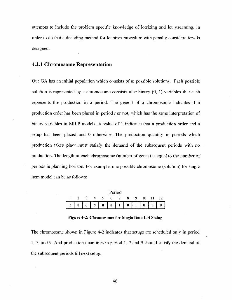
4.2.1 Chromosome Representation
Our GA has an initial population which consists of m possible solutions. Each possible
solution is represented by a chromosome consists of n binary (0, 1) variables that each
represents the production in a period. The gene f of a chromosome indicates if a
production order has been placed in period t or not, which has the same interpretation of
binary variables in MILP models. A value of 1 indicates that a production order and a
setup has been placed and 0 otherwise. The production quantity in periods which
production takes place must satisfy the demand of the subsequent periods with no
production. The length of each chromosome (number of genes) is equal to the number of
periods in planning horizon. For example, one possible chromosome (solution) for single
item model can be as follows:
Period 1 2 3 4 5 6 7 8 9 10 11 12
1 0 0 0 0 0 1 0 1 0 0 0
Figure 4-2: Chromosome for Single Item Lot Sizing
The chromosome shown in Figure 4-2 indicates that setups are scheduled only in period
1, 7, and 9. And production quantities in period 1, 7 and 9 should satisfy the demand of
the subsequent periods till next setup.
46
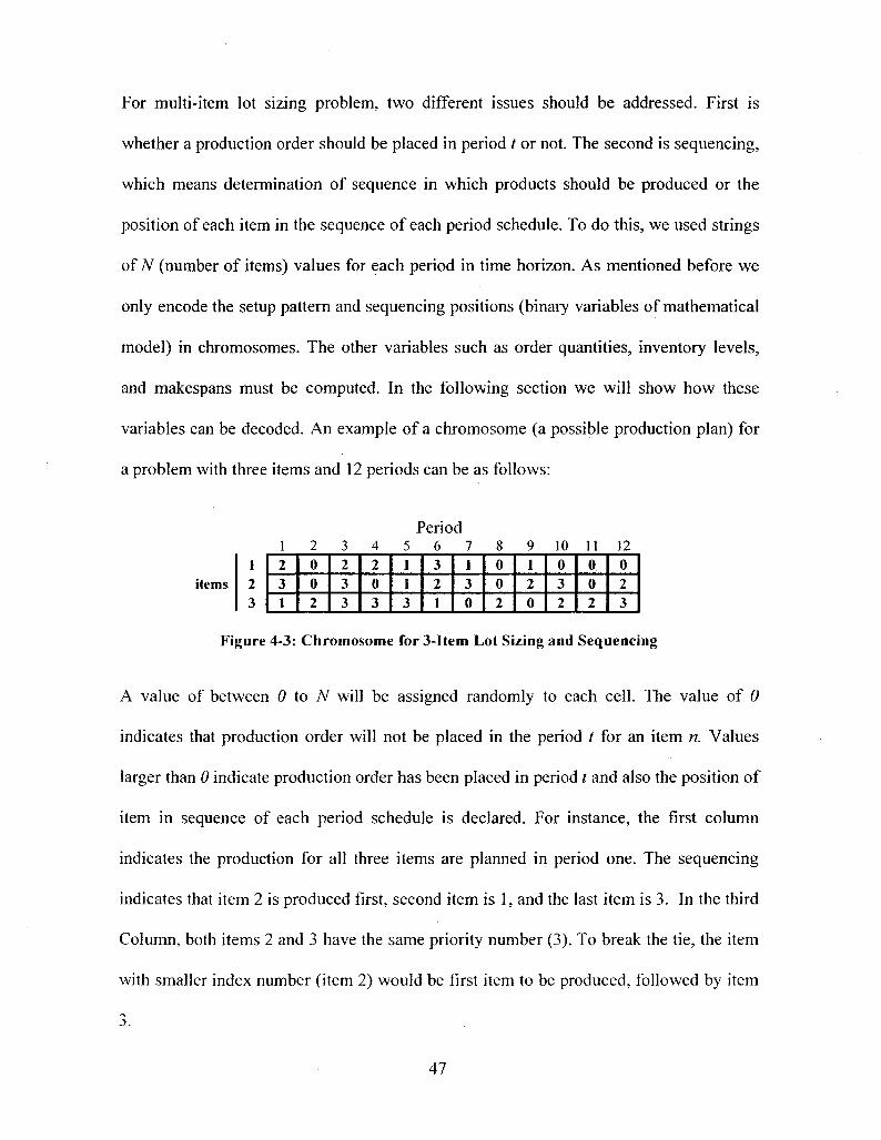
For multi-item lot sizing problem, two different issues should be addressed. First is
whether a production order should be placed in period / or not. The second is sequencing,
which means determination of sequence in which products should be produced or the
position of each item in the sequence of each period schedule. To do this, we used strings
of TV (number of items) values for each period in time horizon. As mentioned before we
only encode the setup pattern and sequencing positions (binary variables of mathematical
model) in chromosomes. The other variables such as order quantities, inventory levels,
and makespans must be computed. In the following section we will show how these
variables can be decoded. An example of a chromosome (a possible production plan) for
a problem with three items and 12 periods can be as follows:
Period 1 2 3 4 5 6 7 8 9 10 11 12 2 3 1
0 0 2
2 3 3
2 0 3
1 1 3
3 2 1
1 3 0
0 0 2
1 2 0
0 3 2
0 0 2
0 2 3
Figure 4-3: Chromosome for 3-Item Lot Sizing and Sequencing
A value of between 0 to N will be assigned randomly to each cell. The value of 0
indicates that production order will not be placed in the period t for an item n. Values
larger than 0 indicate production order has been placed in period t and also the position of
item in sequence of each period schedule is declared. For instance, the first column
indicates the production for all three items are planned in period one. The sequencing
indicates that item 2 is produced first, second item is 1, and the last item is 3. In the third
Column, both items 2 and 3 have the same priority number (3). To break the tie, the item
with smaller index number (item 2) would be first item to be produced, followed by item
47
4.2.2 Decoding Algorithm
The details of orders released, inventory levels of items, and their corresponding
makespan must be determined using a decoding algorithm. The decoding algorithm takes
each chromosome or encoded solution and decodes it into a real solution. Decoding is
performed to determine the order quantities, inventory levels, and makespans. Ultimately,
the total relevant cost is determined by adding inventory holding cost and setup cost.
The decoding algorithm computes the solution as follows: The schedule is generated
backward. It first computes the lot size in last period (7), and then it goes back to period
T-l and continues, until the production decisions are made for all the periods.
Now, consider a period t, when we had made our production decisions for all the
subsequent periods in time horizon. The cumulative demand for each itemy" in period t
(Cdjt) which should be satisfied in period / or its previous periods is equal to the demands
of itemy in subsequent periods minus ordered quantities of itemy in subsequent periods.
(4-2) CdJt=Y.{D]s-Ljs)
The minimum of Cdy, or the quantity of item j that can be produced by the available
capacity of machines will be assigned for production. This means that splitting of demand
is allowed when cumulative demand cannot be completely scheduled for production due
to capacity restrictions. The objective of demand splitting is to increase capacity usage
and reduce the total relevant cost. Before making decision for next item, makespan for
equal number sublots will be calculated and if the makespan exceeds the time bucket the
48
quantity of last item scheduled in the period is reduced by one and the makespan is
recalculated. This procedure continues till a feasible production order is found. Then,
cumulative demand for item j and the residual capacity on machines in the period t will
be updated.
(4-3) RCam,=Caml-fjrjm*L/l 7=1
At this point, the possibility of production and amount of the item with the second
position in the sequence of each period will be checked until decisions are made for the
all items in the period /. The flowchart for the decoding algorithm is shown in figure 4-4
and the pseudo code for algorithm is presented in the appendix 4.
49
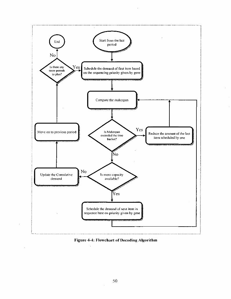
Schedule the demand of first item based on the sequencing priority given by gene
Reduce the amount of the last item scheduled bv one
Schedule the demand of next item in sequence base on priority given by gene
Figure 4-4: Flowchart of Decoding Algorithm
50
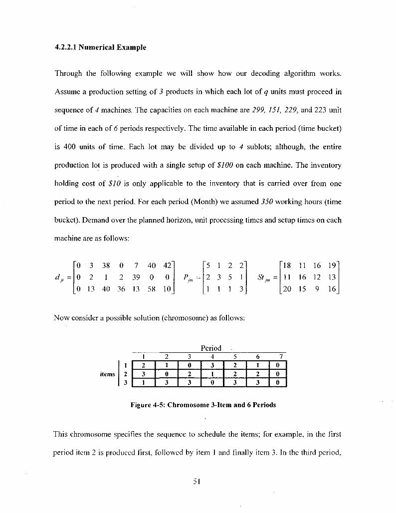
4.2.2.1 Numerical Example
Through the following example we will show how our decoding algorithm works.
Assume a production setting of 3 products in which each lot of q units must proceed in
sequence of 4 machines. The capacities on each machine are 299, 151, 229, and 223 unit
of time in each of 6 periods respectively. The time available in each period (time bucket)
is 400 units of time. Each lot may be divided up to 4 sublots; although, the entire
production lot is produced with a single setup of $100 on each machine. The inventory
holding cost of $10 is only applicable to the inventory that is carried over from one
period to the next period. For each period (Month) we assumed 350 working hours (time
bucket). Demand over the planned horizon, unit processing times and setup times on each
machine are as follows:
d j , =
0 3 38 0 7 40 42
0 2 1 2 39 0 0
0 13 40 36 13 58 10
p» =
5 1 2 2 2 3 5 1
1 1 1 3 stjm =
18 11
20
11 16
15
16 12
9
19 13
16
Now consider a possible solution (chromosome) as follows:
Period
items 1 2 3
2 3 1
1 0 3
0 2 3
3 1 0
2 2 3
1 2 3
0 0 0
Figure 4-5: Chromosome 3-Item and 6 Periods
This chromosome specifies the sequence to schedule the items; for example, in the first
period item 2 is produced first, followed by item 1 and finally item 3. In the third period,
51
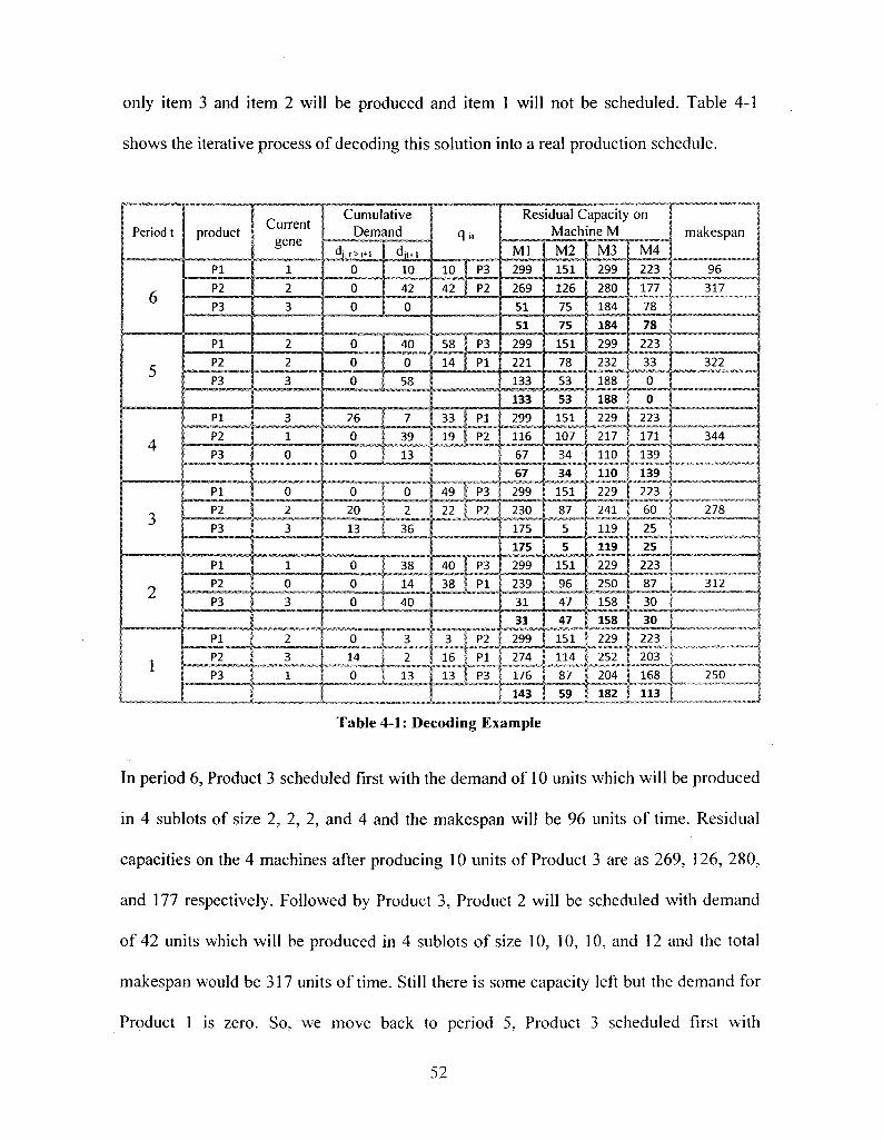
only item 3 and item 2 will be produced and item 1 will not be scheduled. Table 4-1
shows the iterative process of decoding this solution into a real production schedule.
Period t
6
5
4
3
2
1
product
PI
P2
P3
PI
P2
P3
PI
P2
P3
PI
P2
P3
PI
P2
P3 1
PI
P2
P3
Current gene
1
2
3
2
2
3
3
1
_ _ J L _
0
- 2 . 3
1
0
3
Cumulative Demand
^JJJJI>I+II
0
0
0
_ & ! i ' 10
42
0
0 J 40
~*T~~iir" ^ T ^ J ~ 5 8
o h*~ —JL—ILi3™,
0
20
1 13
0
—^1—
° ™t 38
0
14
40 • * • " ' " " " • ' " ' —
* " Y " I 0 ~ ~j_~13 ~
J
q il
™10™T*P3 _ _ ^ _ _ ,
58
14
P3
PI
_ _ _ _ _ _ _
19 P2
4 9 T J E L . L_LL__L
40 P3
I B J P T '
— <
« _ 3
P2
PI
iDP3
Residual Capacity Machine M
Ml 299
269
51
51
299
221
_J33_ 133
_ _ _ _ _ 116
, _ _ .
67
___L
175_
175
299
239
31
31
299
274
176
143
M2 151
126
75
75
151
78
53
53
_J51_ 107
h _ _ i
34
M3 299
280
184
184
299
232
188
188
229
217
110
no ^ 151_ | 229_
' "87** | 241
5
5
151
119
119
229
96 | 250
47
1 4 7 JL_L
158 151 i 229
114 * 252
59 182
on
M4 223
177
78
78
_ 2 2 3 _
33 '
0
0
223
makespan
9 6
317
™ . _ _ _ _ _ _ _
171 ! 344
139
139 . . __ J 223 j ^
""60 f ~278
25 j *
25
223
87 j 312
30 |
30 I
223 i „ _ _
203 _
T 6 8 | 250
113 I
Table 4-1: Decoding Example
In period 6, Product 3 scheduled first with the demand of 10 units which will be produced
in 4 sublots of size 2, 2, 2, and 4 and the makespan will be 96 units of time. Residual
capacities on the 4 machines after producing 10 units of Product 3 are as 269, 126, 280,
and 177 respectively. Followed by Product 3, Product 2 will be scheduled with demand
of 42 units which will be produced in 4 sublots of size 10, 10, 10, and 12 and the total
makespan would be 317 units of time. Still there is some capacity left but the demand for
Product 1 is zero. So, we move back to period 5, Product 3 scheduled first with
52
cumulative demand of 58 units. Makespan is checked and then the capacity is up dated.
The next product in the sequence is Product 1 with total cumulative demand of 40 units.
However, the residual capacity of 33 units of time on machine 4 allows maximum
production of 14 units of Product 1. So, the remaining demand (26 = 40 - 14) should be
produced in the previous periods (1 to 4).
Moving back to period 4, first position belongs to Product 1 with cumulative demand of
33, second position belongs to Product 2 with cumulative demand of 39. However, even
though we have enough capacity we cannot produce 39 unites of Product 2 because the
makespan of producing 33 unites of Product 1 and 39 units of Product 2 (both with 4 sub-
lots) would be larger than the available time bucket (350 units); therefore, in order to find
a feasible schedule, the production quantity of Product 2 should be reduced. Thus, we can
only produce 19 units of Product 2 in period 4 and 20 units remaining demand should be
produced in the previous periods (1 to 3). In the same way, we move backward to period
2 and 1 to decode each chromosome and find the feasible production schedule.
4.2.3 Genetic Algorithm Procedure
The global genetic algorithm continues iteratively until the termination condition is
reached. The termination condition we use for our genetic algorithm is a maximum
generations. This means the GA will stop after of specific number of generations. The
pseudo code for global genetic algorithm is shown in figure 4-6 and the programming
code is presented the appendix 5.
53
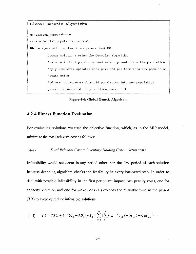
Global Genetic Algorithm
generation number^ 0
create
While
initial population randomly
(g eneration number < max generation) DO
Decode solutions using the decoding algor
Evaluate initial population and select pa
ithm
rents
Apply crossover operator each pair and put them
Mutate child
Add best chromosomes form old population
4- • 1_ ^ A. • 1_
generation number generation number
from
intc
the population
new population
into new populc
+ 1
tion
Figure 4-6: Global Genetic Algorithm
4.2.4 Fitness Function Evaluation
For evaluating solutions we used the objective function, which, as in the MIP model,
minimize the total relevant cost as follows:
(4-4) Total Relevant Cost = Inventory Holding Cost + Setup costs
Infeasibility would not occur in any period other than the first period of each solution
because decoding algorithm checks the feasibility in every backward step. In order to
deal with possible infeasibility in the first period we impose two penalty costs, one for
capacity violation and one for makespans (C) exceeds the available time in the period
(TB) to avoid or reduce infeasible solutions.
M .1
(4-5) T C= TRC + /> * (C, - TB,) + P2 * £ ( £ ((Z.„ • r„ ) + Stjm ) - Capm,) •
54
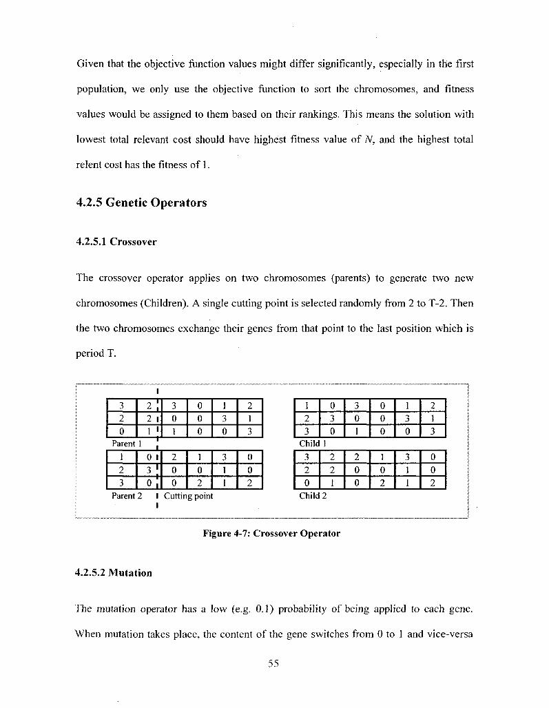
Given that the objective function values might differ significantly, especially in the first
population, we only use the objective function to sort the chromosomes, and fitness
values would be assigned to them based on their rankings. This means the solution with
lowest total relevant cost should have highest fitness value of N, and the highest total
relent cost has the fitness of 1.
4.2.5 Genetic Operators
4.2.5.1 Crossover
The crossover operator applies on two chromosomes (parents) to generate two new
chromosomes (Children). A single cutting point is selected randomly from 2 to T-2. Then
the two chromosomes exchange their genes from that point to the last position which is
period T.
3
2 0
2 ] 2 i
1 l Parent 1 J
1
2 3
0 1
3 '
0 ! Parent 2 1
3 0
1
0 0
0
2
0
0
1
0 2
Cutting point
1
3
0
3
1 1
2
1
3
0
0 2
1
2
3
0
3
0 Child 1
3
2
0
2
2
1 Child 2
3
0 1
2
0
0
0
0
0
1
0 2
1
3
0
3
1 1
2 1
3
0
0
2
Figure 4-7: Crossover Operator
4.2.5.2 Mutation
The mutation operator has a low (e.g. 0.1) probability of being applied to each gene.
When mutation takes place, the content of the gene switches from 0 to 1 and vice-versa
55
(in the single item case). For multi-item problems, when mutation takes place, another set
of random numbers will be assigned to the gene regardless of its original content. Thus,
the mutation operator not only might change the decision of whether or not to produce an
item in particular period; but also, the sequence of items (products) can be changed
randomly in each scheduled period.
4.2.6 Selection Mechanism
In order to be able to regulate selection pressure and population diversity, we used a
combination of ranking and elitist selection mechanisms.
In the proportionate selection chromosomes with high fitness values have higher chances
of being selected and might take over the population, causing premature convergence,
whereas ranking selection results in low convergence. The ranking selection also
maintains the selection pressure in the last generation when the fitness variance is low,
and proved to successfully search the entire solution. We also combined the elitism
mechanism into our search mechanism to keep some of the best individuals in the
population and increase the convergence pressure.
First, we sort current population base on the objective function values and each
chromosome is given a fitness value of 1 to TV (Population size). Then the % of best
chromosomes and their off-springs are copied to the next generation. After copying the
best chromosomes to the next population, the rest of chromosomes are selected by the
ranking mechanism. Genetic operators (crossover and mutation) are applied to generate
the new population. This procedure is repeated for each generation for a specific number
of generations. The pseudo code for the selection mechanism is as follow:
56
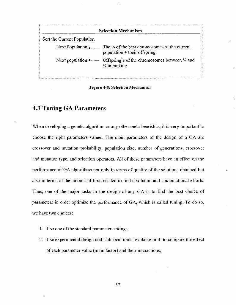
Selection Mechanism
Sort the Current Population
Next Population^ The % of the best chromosomes of the current population + their offspring
Next population < Offspring's of the chromosomes between V* and % in ranking
Figure 4-8: Selection Mechanism
4.3 Tuning GA Parameters
When developing a genetic algorithm or any other meta-heuristics, it is very important to
choose the right parameters values. The main parameters of the design of a GA are
crossover and mutation probability, population size, number of generations, crossover
and mutation type, and selection operators. All of these parameters have an effect on the
performance of GA algorithms not only in terms of quality of the solutions obtained but
also in terms of the amount of time needed to find a solution and computational efforts.
Thus, one of the major tasks in the design of any GA is to find the best choice of
parameters in order optimize the performance of GA, which is called tuning. To do so,
we have two choices:
1. Use one of the standard parameter settings;
2. Use experimental design and statistical tools available in it to compare the effect
of each parameter value (main factor) and their interactions,
57
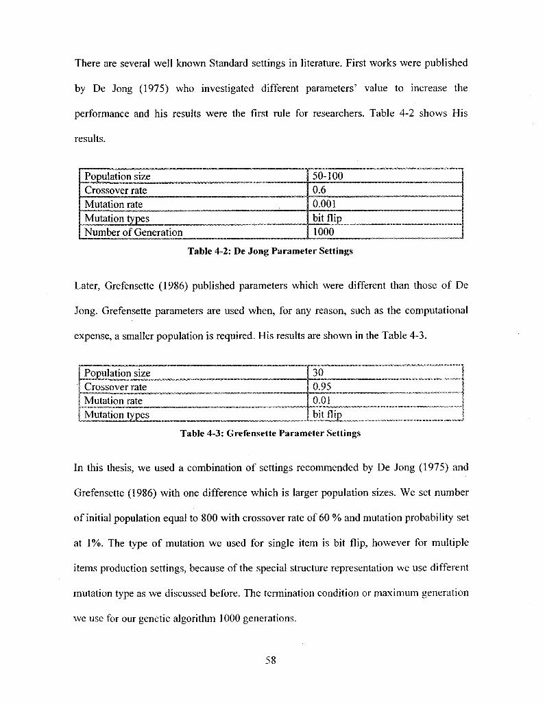
There are several well known Standard settings in literature. First works were published
by De Jong (1975) who investigated different parameters' value to increase the
performance and his results were the first rule for researchers. Table 4-2 shows His
results.
Population size Crossover rate Mutation rate Mutation types Number of Generation
50-100 | 0.6 0.001 bit flip 1000
Table 4-2: De Jong Parameter Settings
Later, Grefensette (1986) published parameters which were different than those of De
Jong. Grefensette parameters are used when, for any reason, such as the computational
expense, a smaller population is required. His results are shown in the Table 4-3.
Population size Crossover rate Mutation rate Mutation types
~"~~IZIIZI IZ I ~** _ _ _ ^ _ _ _ _ _
_ _ _ _ _ _ _ _ ™ ^
[bitflip .... I Table 4-3: Grefensette Parameter Settings
In this thesis, we used a combination of settings recommended by De Jong (1975) and
Grefensette (1986) with one difference which is larger population sizes. We set number
of initial population equal to 800 with crossover rate of 60 % and mutation probability set
at 1%. The type of mutation we used for single item is bit flip, however for multiple
items production settings, because of the special structure representation we use different
mutation type as we discussed before. The termination condition or maximum generation
we use for our genetic algorithm 1000 generations.
58
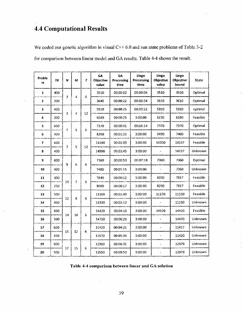
4.4 Computational Results
We coded our genetic algorithm in visual C++ 6.0 and run same problems of Table 3-2
for comparison between linear model and GA results. Table 4-4 shows the result.
Proble m
1
2
3
4
5
6
7
8
9
10
11
12
13
14
15
16
17
18
19
20
TB
400
200
400
200
N
3
3
600 I
400
600
400
600
400
300
250
1 500
400
600
500
600
450
/
7
9
10
12
14
15
• " — — ! )
600 J _ | 1 7
500 1
_ L
M
4
4
5
5
6
7
8
10
12
15
r
6
12
6
12
6
6
6
6
6
6
_ 1
- - — — — — I
GA Objective
value
3510
3640
5910
6540
7370
8350
14180
14990
7360
7480
7840
8000
11160
11330
14420
14710
11420
11570
12980
13550
GA Processing
time
00:00:02
00:00:22
00:00:25
00:00:25
00:00:41
00:01:22
00:01:09
00:03:45
00:00:53
00:01:15
00:00:12
00:00:17
00:01:40
00:02:12
00:04:10
00:06:21
00:04:21
00:05:34
00:06:31
00:09:53
Lingo Processing
time
00:00:04
00:00:54
00:03:22
3:00:00
00:04:14
3:00:00
3:00:00
3:00:00
00:07:18
3:00:00
3:00:00
3:00:00
3:00:00
3:00:00
3:00:00
3:00:00
3:00:00
3:00:00
3:00:00
3:00:00
Lingo Objective
value
3510
3610
5910
6230
7370
9490
14200
-
7360
-
8030
8290
11170
-
14520
-
-
-
-
-
Lingo Objective
bound
3510
3610
5910
6190
7370
7400
14157
14157
7360
7360
7817
7817
11150
11150
14420
14420
11412
11420
12979
12979
State
Optimal
Optimal
optimal
Feasible
Optimal
Feasible
Feasible
Unknown
Optimal
Unknown
Feasible
Feasible
Feasible
Unknown
Feasible
Unknown
Unknown
Unknown
Unknown
Unknown
Table 4-4 comparison between linear and GA solution
59
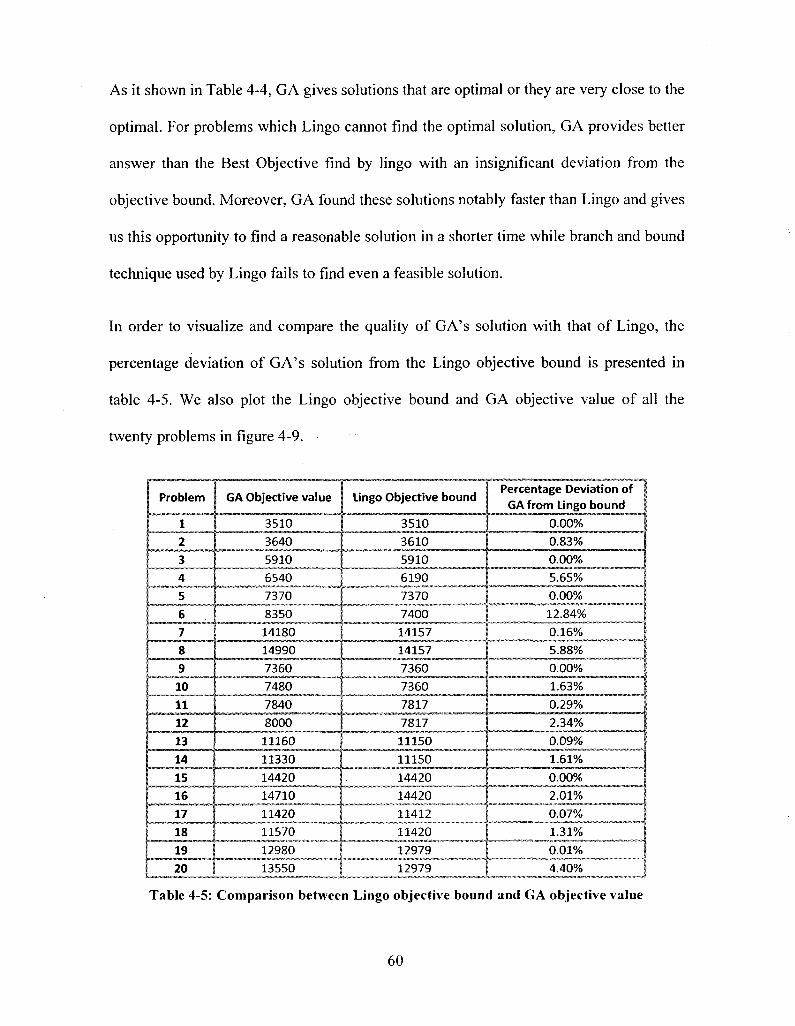
As it shown in Table 4-4, GA gives solutions that are optimal or they are very close to the
optimal. For problems which Lingo cannot find the optimal solution, GA provides better
answer than the Best Objective find by lingo with an insignificant deviation from the
objective bound. Moreover, GA found these solutions notably faster than Lingo and gives
us this opportunity to find a reasonable solution in a shorter time while branch and bound
technique used by Lingo fails to find even a feasible solution.
In order to visualize and compare the quality of GA's solution with that of Lingo, the
percentage deviation of GA's solution from the Lingo objective bound is presented in
table 4-5. We also plot the Lingo objective bound and GA objective value of all the
twenty problems in figure 4-9.
Problem
1
2
3
4
5
6 '
7
8
9
10
11
12
, _ j y t _ 14 15
16
17
18
19 "
20
GA Objective value
3510
3640
5910
6540
7370
8350
14180
Lingo Objective bound
3510
3610
5910
6190
7370
7400
14157
14990 | 14157
7360
7480
7360
7360
7840 I 7817
8000 T~ 7817
11160 _ _ _
11330
11150
11150
14420 1. 14420
14710 1 14420
11420
11570
13550
11412
11420
12979
12979
Percentage Deviation of GA from Lingo bound
0.00%
0.83%
0.00%
5.65%
"o.oo% 12.84%
0.16%
5.88%
0.00%
1.63%
0.29%
2.34%
0.09%
1.61%
0.00% _ J 2.01% 1
0.07% _ _ _ j
1.31% _ J 0.01% 1 4.40% \
Table 4-5: Comparison between Lingo objective bound and GA objective value
60
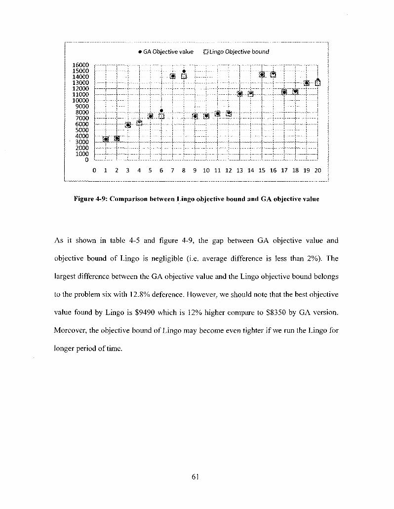
• GA Objective value Q Lingo Objective bound
16000 15000 14000 13000 12000 11000 10000
9000 8000 7000 6000 5000 4000 3000 2000 1000
0
—
»
—
ra
• -
J
r-
I ' in i
^ - . JSL •
_ L i
i !
""I I
* !
| f ~ i
t
i
1 ! •:
;
B - a * — • - - --4- - J — l
i
0 1 2 3 4 5 6 7 8 9 10 11 12 13 14 15 16 17 18 19 20
Figure 4-9: Comparison between Lingo objective bound and GA objective value
As it shown in table 4-5 and figure 4-9, the gap between GA objective value and
objective bound of Lingo is negligible (i.e. average difference is less than 2%). The
largest difference between the GA objective value and the Lingo objective bound belongs
to the problem six with 12.8% deference. However, we should note that the best objective
value found by Lingo is $9490 which is 12% higher compare to $8350 by GA version.
Moreover, the objective bound of Lingo may become even tighter if we run the Lingo for
longer period of time.
61

CHAPTER 5
CONCLUSIONS AND FUTURE WORK
This thesis presents two solution procedures to find the optimal lot size for multiple items
with time varying demand in a multistage production system, when lot streaming and
sequencing are applied simultaneously to ensure orders feasibility and reduce the need for
rescheduling of master production plan. Moreover, it considers machine capacity
constraints, and limited time bucket length, and independent setup times in flowshop
environment.
First, the problem is formulated as a mixed integer linear programming problem (MILP)
and coded with Lingo 10 software. This model takes the demand as an input and gives
the optimal lot size, corresponding sublot size, and the sequence of production as an
output. This model also calculates the makespan in order to ensure that makespan of the
production orders released to shop floor is less than available time in each period. A
small set of problems is generated randomly to test the proposed model. The optimal
solution for small and medium size problems could be found within a reasonable time.
However for larger size problems, because of the NP-hard nature of lot sizing and lot
streaming problems, finding even a feasible solution is hard.
62
Second, a genetic algorithm is developed in order to solve the larger size problems, when
the linear model is unable to function. Then, GA solutions are compared with optimal
solutions and for the larger size problem with the objective bound of linear model. It is
concluded that GA results are acceptable. The proposed genetic algorithm attempts to
include the problem specific knowledge of lotsizing and lot streaming. Because of that,
this genetic algorithm only works on the two binary variables of mathematical model
namely setup pattern and sequencing positions. Then, another heuristic algorithm is used
to decode a solution represented by GA and find the other variables in model like order
quantities, inventory levels, and makespans.
One thing that should be done in future is to use the Experimental Design and the
statistical tools available in it to tune the GA main parameters. The main parameters of
GAs are crossover and mutation probability, population size, number of generations,
crossover and mutation type, and selection operators, which all affect the performance
of GA algorithms not only in terms of quality of the solutions obtained but also in terms
of the amount of time needed to find a solution and computational efforts. Experimental
Design allows us to compare the effect of each parameter value and their interactions.
Another possible future work is to solve more problems to investigate the effect of
different problem configurations like different ratios of holding cost to setup cost, or
different capacity utilization rates on the complexity of the problem.
This thesis only considered independent setup times. However, in presence of dependent
setup times, the limited capacity available for production may be reduced by changeovers
that cause larger setup times; and the need for simultaneous lot sizing and scheduling
63
become more vital. Thus, including the dependent setup times and cost in the model
would make it much more realistic and could be very useful.
Furthermore, like the studies Ho had done between years 1986 and 2005(Ho, 2005; Ho
and law 1995; Ho, 1986). A thorough study of dampening effect of this model and the
impact of it on reduction of the planning instability could be a future work.
64
Bibliography
Adar A. Kalir, S. C. (2001). A near-optimal heuristic for the sequencing problem in
multiple-batch fow-shops with small equal sublots. International Journal of Management
Science, 577-584.
Biskup, D., and Feldmann, M. (2006). Lot streaming with variable sub-lots: an integer
programming formulation. Journal of the Operational Research Society , 296-303.
Campbell, H., Dudek, R., and Smith, M. (1970). A heuristic algorithm for the n-job, m-
machine sequencing problem . Management Science , 630-637.
Chang, J. H., and Chiu, H. N. (2005). A comprehensive review of lot streaming.
International Journal of Production Research , 1515 - 1536.
Cohen, J. (1988). Statistical Power Analysis for Behavioral Science. New York:
Academic Press.
Czarn, A., MacNish, C, Vijayan, K., Turlach, B., and Gupta, R. (2004) Statistical
exploratory analysis of genetic algorithms. IEEE Transaction on Evolutionary
Computation , 405-421.
De Jong, K. (1975). An analysis of behavior of a class of genetic adaptive systems,
Doctoral Thesis, Department of Computer and Communication Sciences. University of
Michigan, Ann Arbor.
Defersha, F. M , and Chen, M. (2008). A Genetic Algorithm for One-Job M-Machine
Flowshop Lot Streaming with Variable Sublots. In the proceeding of the sixth annual
65
international symposium on Supply Chain Management, October 15-17, 2008, Alberta,
Calgary, Canada
Defersha, F. M, and Chen, M, (2008). A hybrid Genetic Algorithm for Flowshop Lot
Streaming with Setup and Variable Sublots. To appear in the International Journal of
Production Research
Defersha, F. M., and Chen, ML, (2006). Lot streaming with variable sub-lots: an integer
programming formulation. Journal of the Operational Research Society (2006) 57, 296—
303,296-303.
Drezner, Z. A. (1984 ). Multi-stage production with variable lot sizes and transportation
of partial lots. European Journal of Operational Research , 221-231.
Goyal, M. A. (2003). On lot streaming in multistage production systems . International
Journal of Production Economics , 195-202.
Goyal, S. K. (1978). Economic batch quantity in a multi-stage production system.
International Journal of Production Research , 267-73.
Graham, R. L. (1966). Bounds for Certain Multiprocessor Timing Anomalies. Bell
System Technical Journal, 1563-1581.
Graham, R., Lawler, E., Lenstr, J., and A. K. (1979). Optimization and approximation in
deterministic sequencing and scheduling. Annals of Discrete Mathematics .
Grefenstette. (1986). Optimization of Control Parameters for Genetic Algorithms. IEEE
Transactions on Systems, Man and Cybernetics , 122-128.
Haase, K., and Kohlmorgen. U. (1996). Parallel genetic algorithm for the capacitated lot-
sizing problem. Karlsruhe : Operations research proceedings.
66
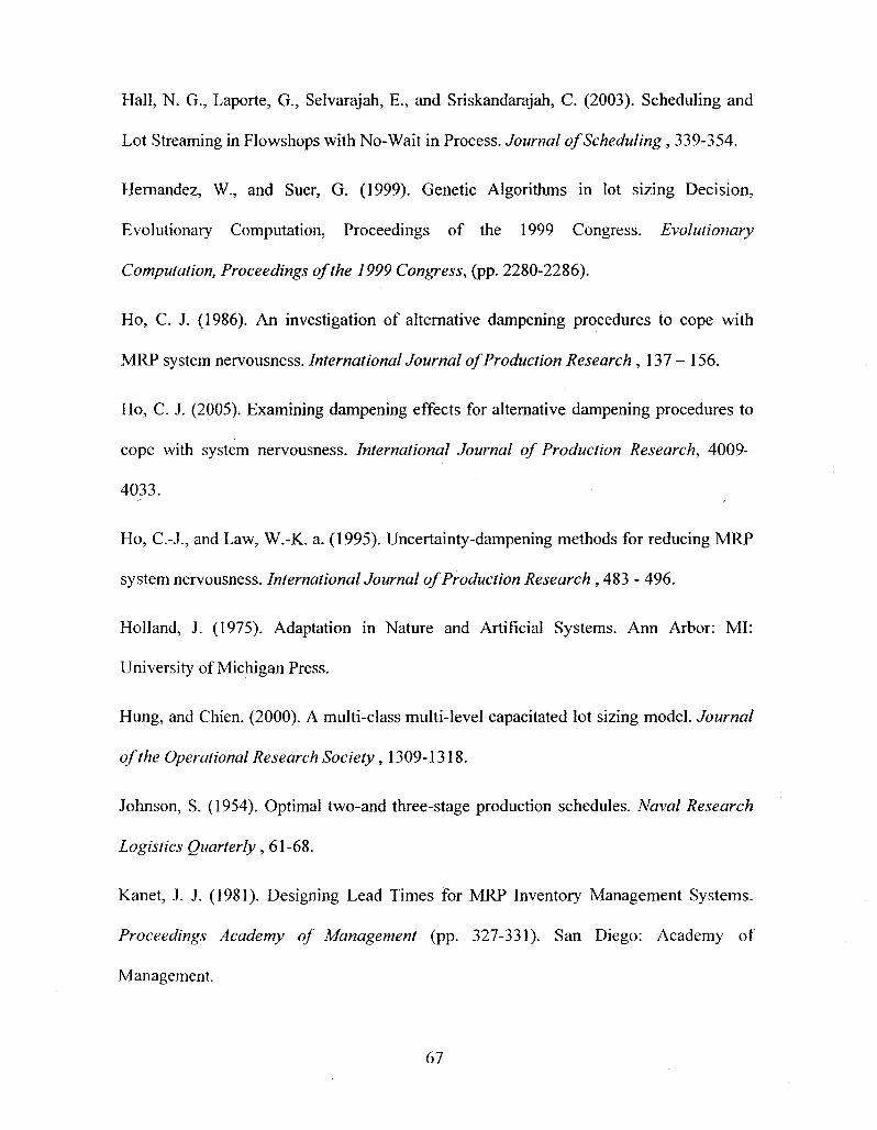
Hall, N. G., Laporte, G., Selvarajah, E., and Sriskandarajah, C. (2003). Scheduling and
Lot Streaming in Flowshops with No-Wait in Process. Journal of Scheduling, 339-354.
Hernandez, W., and Suer, G. (1999). Genetic Algorithms in lot sizing Decision,
Evolutionary Computation, Proceedings of the 1999 Congress. Evolutionary
Computation, Proceedings of the 1999 Congress, (pp. 2280-2286).
Ho, C. J. (1986). An investigation of alternative dampening procedures to cope with
MRP system nervousness. International Journal of Production Research , 137-156.
Ho, C. J. (2005). Examining dampening effects for alternative dampening procedures to
cope with system nervousness. International Journal of Production Research, 4009—
4033.
Ho, C.-J., and Law, W.-K. a. (1995). Uncertainty-dampening methods for reducing MRP
system nervousness. International Journal of Production Research , 483 - 496.
Holland, J. (1975). Adaptation in Nature and Artificial Systems. Ann Arbor: MI:
University of Michigan Press.
Hung, and Chien. (2000). A multi-class multi-level capacitated lot sizing model. Journal
of the Operational Research Society, 1309-1318.
Johnson, S. (1954). Optimal two-and three-stage production schedules. Naval Research
Logistics Quarterly, 61-68.
Kanet, J. J. (1981). Designing Lead Times for MRP Inventory Management Systems.
Proceedings Academy of Management (pp. 327-331). San Diego: Academy of
Management.
67
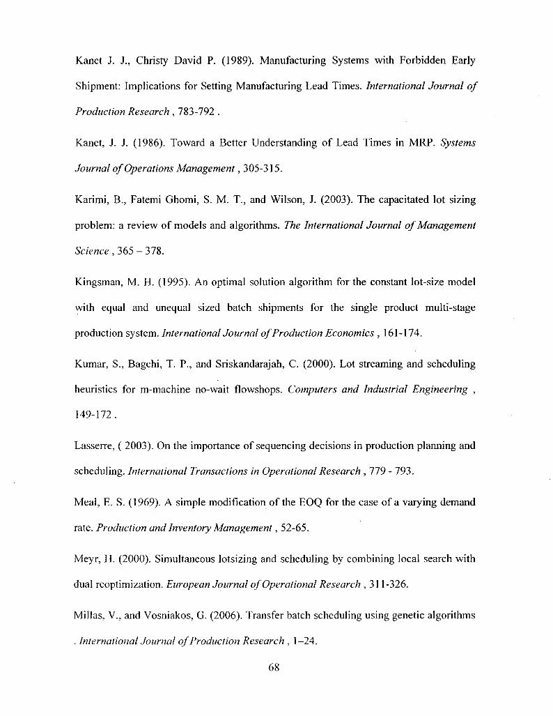
Kanet J. J., Christy David P. (1989). Manufacturing Systems with Forbidden Early
Shipment: Implications for Setting Manufacturing Lead Times. International Journal of
Production Research , 783-792 .
Kanet, J. J. (1986). Toward a Better Understanding of Lead Times in MRP. Systems
Journal of Operations Management, 305-315.
Karimi, B., Fatemi Ghomi, S. M. T., and Wilson, J. (2003). The capacitated lot sizing
problem: a review of models and algorithms. The International Journal of Management
Science , 365 - 378.
Kingsman, M. H. (1995). An optimal solution algorithm for the constant lot-size model
with equal and unequal sized batch shipments for the single product multi-stage
production system. International Journal of Production Economics , 161-174.
Kumar, S., Bagchi, T. P., and Sriskandarajah, C. (2000). Lot streaming and scheduling
heuristics for m-machine no-wait flowshops. Computers and Industrial Engineering ,
149-172.
Lasserre, ( 2003). On the importance of sequencing decisions in production planning and
scheduling. International Transactions in Operational Research , 779 - 793.
Meal, E. S. (1969). A simple modification of the EOQ for the case of a varying demand
rate. Production and Inventory Management, 52-65.
Meyr, H. (2000). Simultaneous lotsizing and scheduling by combining local search with
dual reoptimization. European Journal of Operational Research , 311-326.
Millas, V., and Vosniakos, G. (2006). Transfer batch scheduling using genetic algorithms
. International Journal of Production Research . 1-24.
68
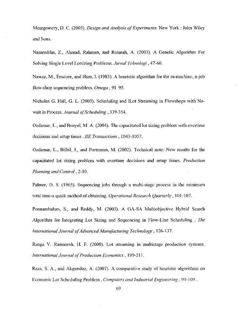
Montgomery, D. C. (2005). Design and Analysis of Experiments. New York : John Wiley
and Sons.
Nasaruddin, Z., Ahmad, Rahman, and Rosmah, A. (2003). A Genetic Algorithm For
Solving Single Level Lotsizing Problems. Jurnal Teknologi, 47-66.
Nawaz, M , Enscore, and Ham, I. (1983). A heuristic algorithm for the m-machine, n-job
flow-shop sequencing problem. Omega , 91-95.
Nicholas G. Hall, G. L. (2003). Scheduling and lLot Streaming in Flowshops with No-
wait in Process. Journal of Scheduling , 339-354.
Ozdamar, L., and Bozyel, M. A. (2004). The capacitated lot sizing problem with overtime
decisions and setup times . HE Transactions , 1043-1057.
Ozdamar, L., Bilbil, I., and Portmann, M. (2002). Technical note: New results for the
capacitated lot sizing problem with overtime decisions and setup times. Production
Planning and Control ,2-10.
Palmer, D. S. (1965). Sequencing jobs through a multi-stage process in the minimum
total time-a quick method of obtaining. Operational Research Quarterly , 101-107.
Ponnambalam, S., and Reddy, M. (2003). A GA-SA Multiobjective Hybrid Search
Algorithm for Integrating Lot Sizing and Sequencing in Flow-Line Scheduling . The
InternationalJournal of Advanced Manufacturing Technology , 126-137.
Ranga V. Ramasesh, H. F. (2000). Lot streaming in multistage production systems.
InternationalJournal of Production Economics , 199-211.
Raza, S. A., and Akgunduz, A. (2007). A comparative study of heuristic algorithms on
Economic Lot Scheduling Problem . Computers and Industrial Engineering , 94-109 .
69
Reiter, S. (1966). A system for managing a job-shop scheduling. Journal of Business .
Sikora, R. (1996). A genetic algorithm for integrating lot-sizing and sequencing in
scheduling a capacitated flow line. Computers and Industrial Engineering , 969-981.
Sikora. R., Chhajed, D., and Shaw, M. J. (1995). Integrating the Lot-Sizing and
Sequencing Decision for Scheduling a Capacitated Flow Line. Computers and Industrial
Engineering, 659-679.
Smith-Daniels, V. L., and Ritzman, L. P. (1988). A model for lot sizing and sequencing
in process industries. International Journal of Production Research , 647 - 674 .
Sriskandarajah, C , and Wagneur, E. (1999). Lot streaming and scheduling multiple
products in two-machine no-wait flowshops. HE Transactions , 695-707.
Sugihara, K. (1997). Measures for performance evaluation of genetic algorithms. Proc.
3rd Joint Conference on Information Sciences . Hawaii.
Szendrovits, A. Z. (1975). Manufacturing cycle time determination for a multi-stage
economic production quantity model. Management Science , 298-308.
Szendrovits, A. Z., and Golden, M. (1984). The effect of two classes of process
organizations on multi-stage production/inventory systems. EFFECT OF TWO CLASSES
Canadian Journal of Operational Research and Information Processing, 40-55.
Wagner, H. M. (1958). Dynamic Version of the Economic Lot Size Model. Management
Science, 89-96.
Xie, J., and Dong, J. (2002). Heuristic genetic algorithms for general capacitated lot-
sizing problem. Computers and Mathematics with Applications , 263-276 .
70
APPENDIX 1: Classification of Lot Sizing Problems
\
1. Planning horizon f
Small buckets
Large buckets
2. Set up Structure f
Simple
Complex
3. Inventory 1
4. Demand |
Lost sales
Backlog
Deterministic
Probabilistic
! !
[
I
Discrete 1
Continues 1
Discrete |
~ ~- _ ^
Continues |
Carr>' over |
Major an minor |
Sequence dependent 1
71
APPENDIX 2: Classification of Lot Streaming Problems
1. System Configuration H
2. Sublot-relate Feature
3. Performance Criterion H
Production Type t-Flow Shop
Job Shop
Open Shop
Arborescent Shop
Number of Products
Single Product
Multi-Product
1 1
Time Model y-
Makespan
Mean Flow Time
Total Flow Time
Mean Tardiness
Number of Tardy
Total Deviation
Cost Model
Total Cost (TC)
Total Cost (TC (C „,„, K)) 1
72
APPENDIX 3: Lingo Code
MODEL: ! MULTI PRODUCTS INTEGRATED LOT STREAMING AND LOT SIZING INTERMINGLING;
SETS: MACHINE/1..12/:CAP; PRODUCT/1..15/; SUBLOT/1..4/; PERIOD/1..7/:C,A_T; UNIT_PROCESSING_TIME(PRODUCT,MACHINE):r PRODUCTION_LOT(PRODUCT, PERIOD):D,Q,Y,I FORMULA1(PRODUCT,SUBLOT,PERIOD):L; FORMULA2(PRODUCT,SUBLOT,MACHINE,PERIOD) FORMULA3(PRODUCT,PRODUCT,PERIOD):X; END SETS
St; E,F;
:P,B;
DATA: A=1000000; SETUP_COST=100; H=10; A_T=600; r=@OLE('C:\Documents and Settings\Data.xls' D=@OLE('C:\Documents and Settings\Data.xls1
st=@OLE('C:\Documents and Settings\Data.xls' CAP=@OLE('C:\Documents @OLE('C:\Documents and @OLE('C:\Documents and ©OLE('C:\Documents and @OLE('C:\Documents and ©OLE('C:\Documents and Settings\Data.xls' END DATA
'Unite_Processing_Time') 'Demand'); , 'Setup_ time');
and Settings\Data.xls','Capacity') Settings\Data.xls','L')=Q; Settings\Data.xls' Settings\Data.xls' Settings\Data.xls'
'Inventory')= 'Sublot_Size' ' v' ) =B ,-•P')=P;
I; )=L;
! OBJECTIVE FUNCTION; ! Minimizing the Total Relevant Cost;
MIN=@sum(PRODUCTION_LOT(j,t):H*I(j,t))+ @sum(PRODUCTION_LOT(j,t):SETUP_COST*Y(j,t));
! SUBJECT TO;
!l; @FOR(PRODUCTION_LOT(j,t) |t#GE#2:I(j,t)=I(j,t-l)+Q(j,t)-D(j,t)) ;
!1-1; @for(PRODUCTION_LOT(j,t):I(j,1)=Q(j,1)); @for(PRODUCTION_LOT(j,t)|t#GE#2:I(j,t-l)>=D(j,t));
!2; ©FOR(MACHINE(m): @FOR(PERIOD(t):
@SUM(PRODUCT(j):Q(j,t)*r(j,m))+ ©SUM(PRODUCT(j):st(j,m)*Y(j,t))<=CAP(m) ));
! 2 - 1 ; ©FOR(PERIOD(t):
C(t) <= A T(t));
!3; @FOR(PRODUCTION_LOT(j,t):Q(j,t)-A*Y(j,t)<=0)
73
!4; @for(PRODUCT)j):
@for(PERIOD(t): @sum (SUBLOT (s) : L (j , s, t) ) =Q (j , t) ) ) ,-
!5; @FOR(F0RMULA2(j,s,m,t):P(j,s,m,t)=L(j,s,t)*r(j,m));
!6; @FOR(MACHINE(m): @FOR(FORMULA3(j,k,t):
Ofor(FORMULA2(j,s,m,t)|j#LT#k :B(j,4,m,t)+P(j,4,m,t)+st(k,m)*Y(k/t)<=B(k/s,m,t) + (l-X(j,k,t))*A) )) ;
!7; ©FOR(MACHINE(m): ©FOR(FORMULA3(j,k,t):
@FOR(FORMULA2(j,s,m,t)|j#LT#k:B(k,4,m,t)+P(k,4,m,t)+st(j,m)*Y(j,t) <=B(j,s,m,t)+X(j,k,t)*A)));
!8; ©FOR(FORMULA2(j,s,m,t) |m#GE#2:B(j,1, m,t)>=B (j , 1, m-1, t)+P (j , l,m-1,t)+st (j,m));
!9; @FOR(FORMULA2(j,s,m,t) :B(j,1,1,t)>=st(j, 1) ) ;
!10; @FOR(F0RMULA2(j,s,ra,t) | m#GE#2 :B (j , s , m, t)>=B(j,s,m-1,t)+P(j,s, m-1, t) ) ;
•11; @FOR(FORMULA2(j,s,m,t) |s#GE#2:B(j , s, m,t)>=B(j,s-l,m,t)+P(j,s-l,m, t) ) ;
! 12 ; @FOR(FORMULA3(j,k,t) :Y(j,t)>=X(j,k,t)) ;
!13; ©FOR(PRODUCTION_LOT(j,t):c(t)>=B(j,4,12,t)+P(j,4,12,t)) ;
!15; @for(PRODUCTION_LOT(j,t):@BIN(Y(j,t)));
!16; @FOR(FORMULA3(j,k,t) |j#LT#k:@BIN(X(j,k,t))) ;
! Integer; @FOR(FORMULAl(j,S,t):@GIN(L(j,S,t)));
Icostant sublot size;
!@F0R(F0RMULA1(j,S,t) |s#GE#2 #AND# S#LE#3:L(j,S,t)=L(j,s-1,t) ) ;
!@FOR(FORMULAl(j,S,t)|s#EQ#4:L(j,s,t)>=L(j,s-l,t));
74
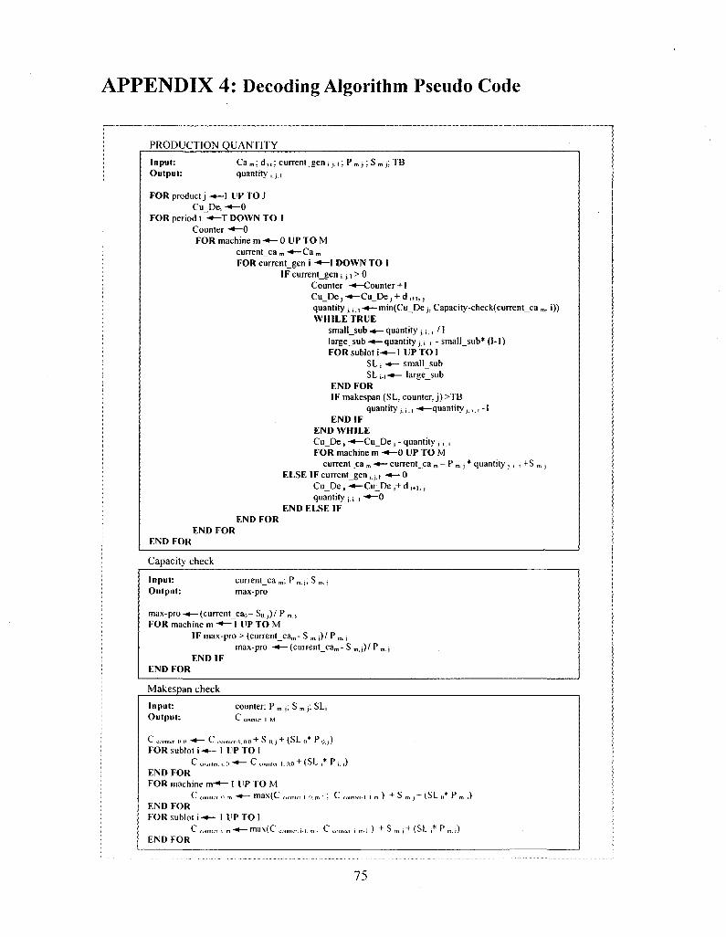
APPENDIX 4: Decoding Algorithm Pseudo Code
PRODUCTION QUANTITY
Input: Output:
Ca m; d j , ; currentgen ;. j. i; P , quantity -, , i
:TB
FOR product j - * - l UP TO J CuDej - * -0
FOR period t -*-T DOWN TO 1 Counter -•—0 FOR machine m -*- 0 UP TO M
currentca m -*—Ca m
FOR current gen i •*- ! DOWN TO 1 IF currentgen j j.i > 0
Counter -*—Counter + 1 Cu_De j -»-Cu De j + d ,„,,}
quantity jTi,,-*—min(Cu_Dei, Capacity-check(current_ca „. i)) WHILE TRUE
smallsub -<— quantity; t\,, /1 largesub -•—quantity j iS , - smallsub* (1-1) FORsubloti-*—1 UPTOl
SL i -«— smallsub SL i_i-<— largesub
END FOR IF makespan (SL. counter, j) >TB
quantity j, \., -*—quantity , , , -1 END IF
END WHILE CuDe j •*—CuDe , - quantity ; , , FOR machine m - * - 0 UP TO M
currentca m -*— currentca m - P m j * quantity j, i , +S m , ELSE IFcurrentgen , j j -*—0
Cu_De j •*— Cu_De ,+ d I+1,, quantity j i i •*— 0
END ELSE IF END FOR
END FOR END FOR
Capacity check
Input: current ca „,; P m j ; S m j
Output: max-pro
max-pro -*— (current cao- So.j)/ P m. i FOR machine m -*— 1 DP TO M
IF max-pro > (current_cam- S m j)/ Pm.j max-pro -«—(current ca„,-S„
END IF END FOR
i ' P . ,
Makespan check
Input: Output:
*~ counter. 0. 0 ^ *~
FOR sublot i -*— C olunk,
END FOR FOR machine rrr"
C END FOR FOR sublol i - * -
r *- inunii'r END FOR
counter: P m ,; S m ,: SL, *- cimnler. 1 M
,«-,.i.ao + S „ . l + ( S L 0 * P 0 , ) 1 U P T O I i. 0 ~< C counltT-l. 0.0 + ( S L j * P j . j )
• - 1 UP T O M o. m -•— max(C n „ i „ . k n „,.,: C „„,
1 I T TO 1 . m -*— max(C 0,„„ur. i i . m ; C 0 , „„„ .
w-I.l.m) + S m j + ( S L „ * P m . ; )
, „ . , ) + S „ , , + (SL,*P i n . , )
75
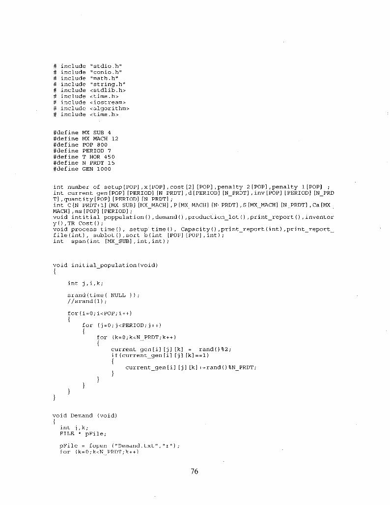
# include "stdio.h" # include "conio.h" # include "math.h" # include "string.h" # include <stdlib.h> # include <time.h> # include <iostream> # include <algorithm> # include <time.h>
#define MX SUB 4 #define MX MACH 12 #define POP 800 #define PERIOD 7 #define T HOR 450 #define N PRDT 15 #define GEN 1000
int number of setup[POP],x [POP],cost [2] [POP],penalty 2[POP],penalty 1 [POP] ; int current gen[POP] [PERIOD] [N PRDT] ,d[PERIOD] [N_PRDT] ,inv[POP] [PERIOD] [N_PRD T],quantity[POP][PERIOD][N PRDT]; int C[N PRDT+1] [MX SUB] [MX_MACH] ,P [MX_MACH] [N_PRDT] ,S[MX_MACH] [N_PRDT] ,Ca [MX_ MACH] ,ms [POP] [PERIOD] ; void intitial poppulation(),demand(),production_lot(),print_report(),inventor y() ,TR CostO ; void process timet), setup timed, Capacity(),print_report(int),print_report_ file(int), sublot() ,sort b(int [POP] [POP] ,int) ; int span(int [MX_SUB],int,int);
void initial_population(void)
int j,i,k;
srand(time( NULL ) ) ,-//srand(l);
for (i = 0;i<POP,-i + + ) {
for (j = 0;j<PERIOD;j + + ) {
for (k=0;k<N PRDT;k++) {
c u r r e n t g e n [ i ] [ j ] [ k ] = rand()%2; i f ( c u r r e n t g e n [ i ] [ j] [k]= = l ) {
c u r r e n t _ g e n [ i ] [j] [k]+=rand()%N_PRDT;
void Demand (void) { int j,k; FILE * pFile;
pFile = fopen ( "Demand . txt ", "r" ) ,-for (k=0;k<N PRDT;k++)
76
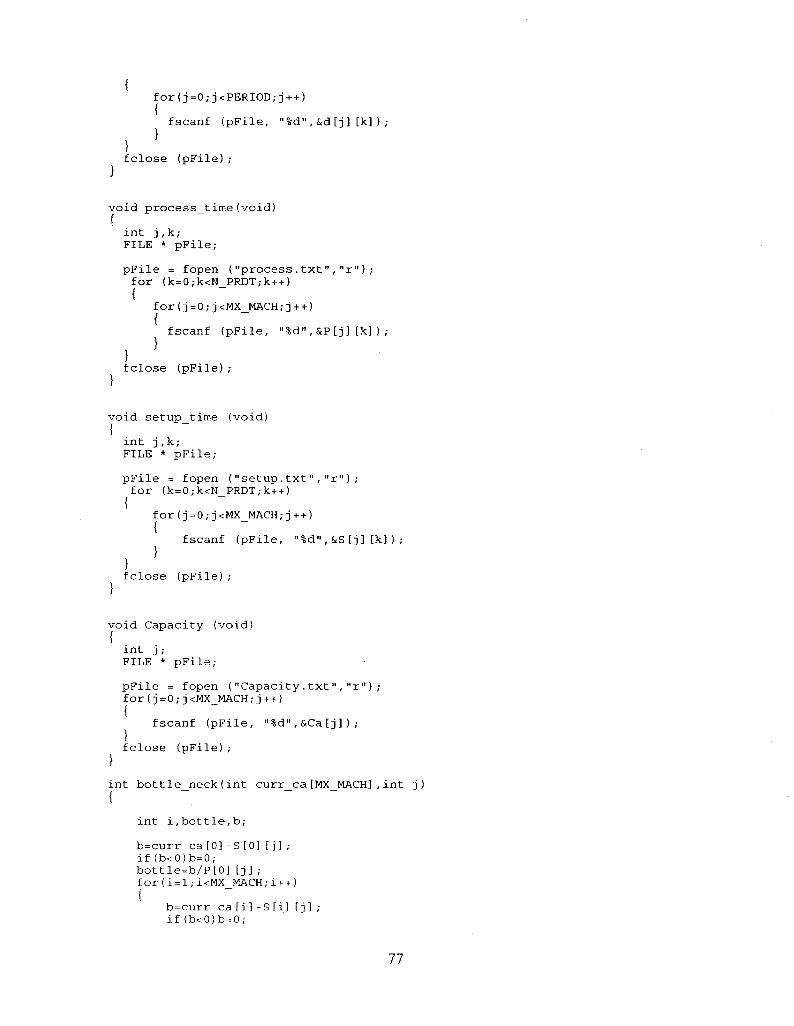
{ for(j=0;j<PERIOD;j++)
{ fscanf (pFile, "%d",&d[j][k]);
fclose (pFile); }
void process time(void)
{ int j,k; FILE * pFile;
pFile = fopen ("process.txt","r"); for (k=0;k<N PRDT;k++)
{ for(j=0;j<MX MACH;j++)
{ fscanf (pFile, "%d",&P [j] [k]);
fclose (pFile); }
void setup time (void)
{ int j,k; FILE * pFile;
pFile = fopen ("setup.txt","r"); for (k=0;k<N PRDT;k++)
{ for(j=0;j<MX MACH;j++)
{ f s c a n f ( p F i l e , "%d" , &S [ j ] [k] ) ,-
f c l o s e ( p F i l e ) ;
void Capacity (void)
{ int j ; FILE * pFile;
pFile = fopen ("Capacity.txt","r"); for (j = 0;j<MX MACH;j+ + )
{ fscanf (pFile, "%d",&Ca [j]);
} fclose (pFile);
} int bottle neck(int curr ca[MX MACH],int j) {
int i,bottle,b;
b = c u r r c a [ 0 ] - S [ 0 ] [ j ] ; i f ( b < 0 ) b = 0 ; b o t t l e = b / P [ 0 ] [ j ] ; f o r ( i = l ; i < M X MACH;i++) {
b = c u r r c a [ i ] - S [ i ] [ j ] ; i f ( b < 0 ) b = 0 ;
77
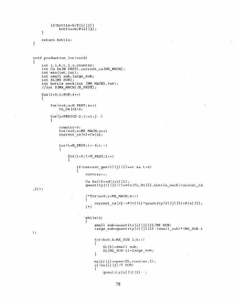
i f ( b o t t l e > b / P [ i ] [ j ] ) b o t t l e = b / P [ i ] [ j ]
return bottle;
void production lot(void) {
int j,i,k,t,1,z,counter; i n t Cu De[N PRDT],current_ca[MX_MACH]; i n t m i n ( i n t , i n t ) ; int small sub,large_sub; int SL [MX SUB] ; i n t b o t t l e n e c k ( i n t [MX M A C H ] , i n t ) ; / / i n t S[MX_MACH][N_PRDT];
f o r ( i = 0 ; i < P O P ; i + + )
f o r ( z = 0 ; Z < N PRDT;Z++) Cu_De [ z ] = 0 ;
f or'( j =PERIOD-2 ; j > = 1 ; j - - ) {
c o u n t e r = 0 ; for(z=0;Z<MX MACH;z++) c u r r e n t c a [ z ] = C a [ z ] ;
for(t=N PRDT;t>=0;t--) {
for(l=0;l<N PRDT;l++) {
.1));
if(current gen[i][j][l]==t && t>0) {
counter++ ,-
Cu D e [ l ] + = d [ j + l ] [1] ,-q u a n t i t y [ i ] [ j ] [ 1 ] = m i n ( C u _ D e [ 1 ] , b o t t l e _ n e c k ( c u r r e n t _ c a
/ * fo r ( z=0 ;Z<MX MACH;Z++) {
c u r r e n t c a [ z ] - = P [ z ] [ 1 ] * q u a n t i t y [ i ] [ j ] [1]+S [z] [1] ; } * /
w h i l e ( l ) {
s m a l l s u b = q u a n t i t y [ i ] [ j ] [ 1 ] / M X SUB; l a r g e _ s u b = q u a n t i t y [ i ] [ j ] [ 1 ] - ( s m a l l _ s u b ) * ( M X _ S U B - 1
for(k=0;k<MX SUB- l ;k++) {
SL [k] =smal 1 s u b ,-SL[MX_SUB-1]= la rge_sub ;
nns [ i ] [ j ] =span (SL, c o u n t e r , 1) i f ( m s [ i ] [j]>T_HOR) {
q u a n t i t y t i ] [ j ] [1] - - ;
78
} e l s e {
Cu D e [ l ] - = q u a n t i t y [ i ] [ j ] [ 1 ] ; b reak ;
f o r ( z = 0;z<MX MACH,-z + + ) {
c u r r e n t ca [z ] -=P[z ] [1] * q u a n t i t y [i] [j] [1]+S[z] [1] }
} e l s e i f ( c u r r e n t gen [ i ] [j] [ l ]==t && t==0) {
Cu De[ l ]+=d[ j + l ] [1] ; q u a n t i t y [ i ] [j] [1]=0;
} } / / end of p roduc t seq s e a r c h ( l )
}//end of s e q ( t ) }//end of p e r i o d ( j )
/ / f i r s t month j = 0; counter=0; for(t=N PRDT;t>=0;t-
fo r ( l=0 ; l<N PRDT/1++) {
i f ( cu r ren t g e n [ i ] [j] [ l ]==t) {
counter++;
Cu De[ l ]+=d[ j+ l ] [1] ; q u a n t i t y [ i ] [ j] [l]=Cu_De[l] ;
small s u b = q u a n t i t y [ i ] [ j ] [ 1 ] / M X SUB; la rge_sub=quant i ty [ i ] [ j ] [1 ] - ( smal l_sub)*(MX_SUB-1)
for(k=0;k<MX SUB-l;k++) {
/*SL[k]=smal l sub; SL[MX SUB-l]=large s u b ; * / SL[k]=large sub; SL[MX_SUB-1]=small_sub;
}
ms[i] [j]=span(SL,counter,1);
} }// end of product seq search(1)
}//end of seq(t)
}//end of pop(i)
void inventory()
int j,i,1,z;
for(i=0;i<POP;i++) {
79
} }
f o r ( z = 0 ; z < N PRDT;z++) {
i n v [ i ] [0] [ z ] = g u a n t i t y [ i ] [0] [z] ; / / - d [ 0 ] [z] ; }
f o r ( j = l ; j < P E R I O D ; j + + ) {
f o r ( l = 0 ; l < N PRDT;l++) {
i n v [ i ] [ j ] [1]= i n v [ i ] [ j - 1 ] [1]+ q u a n t i t y [ i ] [ j ] [ l ] - d [ j ] [1] }
}
i n t m a x ( i n t a , i n t b) {
i n t o u t p u t ; o u t p u t = a ; i f ( b > a )
o u t p u t = b ; r e t u r n o u t p u t ;
}
i n t m i n ( i n t a , i n t b) {
int output; output=a; if(b<a)
output=b; return output;
int span (int SL [MX SUB],int counter,int 1) {
int max(int,int); int i, j;
C [ c o u n t e r ] [0] [0]=C [ c o u n t e r - 1 ] [MX_SUB-1] [0 ]+S[0 ] [1] + ( S L [ 0 ] * P [ 0 ] [1] ) ; f o r ( i = l ; i < M X SUB;i++) {
C [ c o u n t e r ] [ i ] [0] = C [ c o u n t e r ] [ i - 1 ] [0] + ( S L [ i ] * P [ 0 ] [1] ) ; }
f o r ( j = 1 ; j <MX_MACH;j ++) {
C [ c o u n t e r ] [0] [ j ] = m a x ( C [ c o u n t e r ] [0] [ j - 1 ] , C [ c o u n t e r - 1 ] [MX_SUB-1] [ j ] ) + S [ j ] [ l ] + ( S L [ 0 ] * P t j ] [1]) ;
}
f o r ( i = l ; i < M X _ S U B ; i + + ) {
f o r ( j = l ; j < M X MACH;j++) {
C [ c o u n t e r ] [ i ] [ j ] = m a x ( C [ c o u n t e r ] [ i - 1 ] [ j ] , C [ c o u n t e r ] [ i ] [ j - 1 ] ) + S L [ i ] * P [ j ] [1] ;
} } r e t u r n C [ c o u n t e r ] [MX SUB-1] [MX MACH-1] ;
v o i d TR C o s t ( v o i d )
80
int i, j,1,z; int TCU[MX_MACH];
for(i=0;i<POP;i++) {
number of setup [i]=0; for(j=0;j<PERIOD;j++) {
for(l=0;l<N PRDT;l++) {
i f ( q u a n t i t y [ i ] [ j ] [ 1 ] > 0 ) n u m b e r _ o f _ s e t u p [ i ] + = 1 ;
}
for(i=0;i<POP;i++) {
x[i]=0; for(j=0;j<PERIOD;j++) {
for(l=0;l<N PRDT/1++) {
x [ i ] + = i n v [ i ] [ j ] [1] ; }
f o r ( i = 0 ; i < P O P ; i + + ) {
p e n a l t y 2 [ i ] = 0 ; f o r ( j = 0 ; j < P E R I O D ; j + + ) {
i f ( m s [ i ] [ j ] > T HOR) p e n a l t y 2 [ i ] + = m s [ i ] [ j ] - T HOR;
} p e n a l t y 1 [ i ] = 0 ; f o r ( j = 0 ; j < P E R I O D ; j + + ) {
for(z=0;Z<MX MACH;z++)
TCU[z]=0; for(1=0;1<N_PRDT;1++)
{ i f ( q u a n t i t y [ i ] [ j ] [1]>0)
T C U [ z ] + = q u a n t i t y [ i ] [ j ] [ l ] * P [ z ] [1]+ S [z] [1] }
i f ( T C U f z ] > C a [ z ] ) p e n a l t y _ l [ i ] + = T C U [ z ] - C a [ z ] ;
c o s t [0] [ i ] = i ; c o s t [1] [ i ] = x [ i ] * 1 0 + n u m b e r _ o f _ s e t u p [ i ] * 1 0 0 + p e n a l t y _ 2 [ i ] * 5 0 0 0 + p e n
a l t y 1 [ i ] * 5 0 0 0 ; . }
v o i d p r i n t r e p o r t ( i n t genno) {
81

int i,j,k,t;
printf("Process time on machine j:\n") for(j=0;j<MX MACH;j++)
{ for (k=0;k<N PRDT;k++) printf("%4d", P[j][k]); printf("\n");
printf("\n\n");
printf("Setup time on machine j: \n") for(j = 0;j <MX_MACH;j + +)
for (k=0;k<N PRDT;k++) printf("%4d", S[j][k]);
printf ("\n");
printf ("\n\n") ,-
printf ( "Capacity of machine j: \n"),-for(j=0;j<MX MACH;j++)
{ printf("%6d", Ca [j]) ;
printf("\n\n");
for(i=0;i<POP;i++) {
printf {" \n") printf (" \n") printf("Generation: %d\n",genno); printf (" \n") printf (" \n")
printf("Chromosome %d\n",i); for (k=0;k<N PRDT;k++) {
for(j=0;j<PERIOD;j++) p r i n t f ("%5d" , cu r ren t_gen [ i ] [j] [k] ) ,-printf("\n");
} printf("\n"); printf("Demand for Products :" "\n\n" ) ,-printf(" Jan Feb Mar April May Jun July " " \ n " ) ;
for (k=0;k<N PRDT;k++)
{ for(j=0;j<PERIOD;j++) printf ("%5d" ,d [j] [k] ) ,-printf("\n");
} printf("\n"); printf("Order Released for each Product:""\n\n"); printf(" Jan Feb Mar April May Jun July ""\n"); for (k=0;k<N PRDT;k++)
{ for(j=0;j<PERI0D;j++) printf ("%5d" .quantity [i] tj] [k] ) ,-
82
printf("\n");
printf("\n");
printf("Makespans:""\n\n"); for(j =0;j<PERIOD;j ++) {
pr in t f ("%5d", m s t i l t j l ) ; p r i n t f ( " \ n \ n " ) ;
printf ("Inventory of each product at the end of each period:""\n\n") ; printf(" Jan Feb Mar April May Jun July ""\n"),-for (k=0;k<N PRDT;k++) {
for(j=0;j<PERI0D;j++) printf("%5d",inv[i][j][k]); printf("\n");
} printf("\n");
printf ("\n \n ") ; printf("number of setups %4d",number_of_setup [i]); printf("\n"),-printf("total Inventory %4d",x[i]); printf("\n"); p r i n t f ( " C a p a c i t y v i o l a t i o n Pena l t y % 4 d " , p e n a l t y _ l [ i ] ) ; p r i n t f ("\n") ,-printf("time horizon Penalty %4d" ,penalty_2 [i] ) ,-printf ("\n") ,-for(t=l;t<P0P;t++)
if(cost [0] [t]==i) printf("total relevant cost $%4d",cost [1] [t]) ;
printf("\n"); printf("\n\n\n");
void print_report_file(int genno)
int i,j,k,t; FILE *report;
report=fopen("report.txt","w");
fprintf (report, "Process time on machine j:\n" ),-for(j = 0;j <MX_MACH;j + + )
for (k=0;k<N PRDT;k++) fprintf (report, "%4d", P[j] [k] ) ,-fprintf(report,"\n");
} fprintf(report,"\n\n");
fprintf(report,"Setup time on machine j: \ n " ) ; for(j=0;j<MX MACH;j++) { for (k=0;k<N PRDT;k++)
f p r i n t f ( r e p o r t , "%4d", S [ j ] [k]) ; f p r i n t f ( r e p o r t , " \ n " ) ;
fprintf(report,"\n\n");
83
fprintf(report,"Capacity of machine j: \n") for(j=0;j<MX MACH;j++)
{ fprintf(report,"%6d", Ca[j]),-
} fprintf(report,"\n\n");
for (i = 0,-i<POP;i + + )
{
f print f (report," \n") ; fprintf (report, " \n") ; fprintf(report,"Generation: %d\n",genno); fprintf (report, " \n") ; fprintf (report," \n" ) ,-
fprintf(report,"Chromosome %d\n",i); for (k=0;k<N PRDT;k++)
{ for(j=0;j<PERIOD;j++) f p r i n t f ( r e p o r t , " % 5 d " , c u r r e n t _ g e n [ i ] [ j ] [ k ] ) ; fprintf(report,"\n");
} fprintf(report,"\n"); fprintf(report,"Demand for Products:""\n\n"); fprintf (report, " Jan Feb Mar April May Jun July ""\n"),-for (k=0;k<N PRDT;k++)
{ for(j=0;j<PERIOD;j++) fprintf(report,"%5d",d[j][k] ) ; fprintf (report, "\n" ) ,-
} fprintf(report,"\n"); fprintf(report,"Order Released for each Product:""\n\n"),-fprintf(report," Jan Feb Mar April May Jun July ""\n"); for (k=0,-k<N PRDT;k+ + )
{ for(j=0;j<PERIOD;j++) fprintf(report,"%5d",quantity [i] [j] [k] ) ; fprintf(report,"\n");
} fprintf(report,"\n"); fprintf(report,"Makespans:""\n\n"),-for(j=0;j<PERIOD;j++)
{ fprintf(report,"%5d", ms[i] [j]);
} fprintf(report,"\n\n"); fprintf(report,"Inventory of each product at the end of each period:"
"\n\n"); fprintf(report," Jan Feb Mar April May Jun July ""\n"); for (k=0;k<N PRDT;k++)
{ for(j=0;j<PERIOD;j++) fprintf(report,"%5d",inv[i][j][k]); fprintf(report,"\n");
} fprintf(report,"\n");
fprintf (report ,"\n \
84
n") ; fprintf(report,"number of setups %4d",number_of_setup [1J) ; fprintf(report,"\n"); fprintf(report,"total Inventory %4d",x [i]); fprintf(report,"\n"); fprintf(report,"Capacity violation Penalty %4d" ,penalty_l [i] ) ,-fprintf(report,"\n"); fprintf(report,"time horizon Penalty %4d",penalty_2 [i]) ; fprintf(report,"\n"); for(t=l,-t<POP;t++)
if(cost [0] [t]==i) fprintf(report,"total relevant cost $%4d",cost[1][t]);
fprintf(report,"\n"); fprintf(report,"\n\n\n");
void sort b(int list [POP] [POP],int count) {
int i,j,temp; for(i=0;i<count;i++)
for(j=count;j>=i;--j) i f ( l i s t [1] [ j - l ] > l i s t [ l ] [ j ] ) {
t e m p = l i s t [ 0 ] [ j - 1 ] ; l i s t [0] [ j - l ] = l i s t [0] [ j ] ; l i s t [0] [ j ] = t e m p ; t e m p = l i s t [ 1 ] [ j - 1 ] ; l i s t [1] [ j - l ] = l i s t [ l ] [ j ] ; l i s t [1] [ j ] = t e m p ;
}
v o i d g e n ( ) {
i n t i , j , c u r r e n t _ g e n _ n e x t [ P O P ] [PERIOD] [N_PRDT] , p a r e n t 1 , p a r e n t 2 , 1 , r a n d o m _ b a d , b a d s [ P O P / 4 ] ;
/ / s o r t s o r t _ b ( c o s t , P O P - 1 ) ;
/ / c r o s s o v e r f i r s t b e s t 1/4 f o r ( i = 0 ; i < ( P O P / 4 ) ; i + = 2 ) {
p a r e n t l = c o s t [0] [ i ] ; p a r e n t 2 = c o s t [0] [ i+1] ;
f o r ( j = 0 ; j < P E R I O D ; j + + ) {
f o r ( l = 0 ; l < N PRDT/1++) {
c u r r e n t gen n e x t [ i ] [ j ] [1] ^ c u r r e n t g e n [ p a r e n t l ] [ j ] [1] ; c u r r e n t _ g e n _ n e x t [ i + 1] [ j ] [1] = c u r r e n t _ g e n [ p a r e n t 2 ] [ j ] [1] ,-
}
for(j=0;j<PERI0D;j++) if(j<(PERIOD/2))
{ for(l = 0;l<N PRDT.-1 + +)
{ c u r r e n t _ g e n _ n e x t [ ( P O P / 4 ) + i ] [ j ] [ 1 ] = c u r r e n t _ g e n [ p a r e n t l ] [ j ]
[1] ; c u r r e n t _ g e n _ n e x t [ ( P O P / 4 ) + l + i ] [ j ] [ 1 ] = c u r r e n t _ g e n [ p a r e n t 2 ] [
j ] [1] ;
85
[ 1 ] ;
j ] t l ]
e l s e {
fo r ( l=0 ; l<N PRDT;1++) {
cur ren t_gen_next [ (POP/4)+i ] [ j] [1 ]=cur ren t_gen[paren t2 ] [j] cur ren t_gen_next [ (POP/4)+l + i ] [j] [1]=current_gen [ p a r e n t l ] [
//version 1 for(i=P0P/2;i<P0P;i++)
for(j=0;j<PERIOD;j++) for(l=0;l<N PRDT;l++)
c u r r e n t _ g e n _ n e x t [ i ] [ j ] [ 1 ] = c u r r e n t _ g e n [ i - P O P / 4 ] [ j ] [ 1 ] ;
/ / v e r s i o n 2 / * fo r (i=P0P/2,-i< (3*P0P/4) ; i + +)
for(j=0;j<PERIOD;j++) fo r ( l=0 ; l<N PRDT/1++)
c u r r e n t g e n _ n e x t [ i ] [ j ] [ 1 ] = c u r r e n t _ g e n [ i - P O P / 4 ] [ j ] [ 1 ] ; for ( i=0; i<POP/4; i++) {
random bad=rand()%(POP/2)+POP/2; for(j=0;j<i;j++)
if(badstj]==random bad)
{ random_bad=rand()%(POP/2)+P0P/2; j = -l;
} bads[j]=random bad;
} for(i=(3*POP/4) ; i<POP;i + + )
for(j=0;j<PERIOD;j++) fo r ( l=0 ; l<N PRDT;l++)
cur ren t_gen_nex t [i] [j] [1 ]=cur ren t_gen[bads [ i - (3*POP/4) ] ] [j] [1
/ / change g e n e r a t i o n s for( i=0; i<POP;i++)
for(j=0;j<PERIOD;j++) fo r ( l=0 ; l<N PRDT;l++)
cu r ren t_gen [ i ] [j] [1] =current_gen_next [ i ] [ j] [1] ,-
/ / m u t a t i o n for ( i = 0;i<POP,-i + + )
for(j=0;j<PERIOD;j++) fo r ( l=0 ; l<N PRDT;l++)
if(rand()%25==0) {
c u r r e n t g e n [ i ] [ j ] [ 1 ] = r a n d ( ) % 2 ; i f ( c u r r e n t gen [ i ] [ j ] [1]= = 1)
current_gen[ i ] [ j ] [1]+=rand()%N_PRDT;
vo id main(void) {
i n t i ; time t s t a r t , e n d ;
86
start = time (NULL);
printf("Generating initial population.\n"); initial population(); Demand () ,-setup time () ,-process time (),-Capacity!),-
printf("running the GA\n"); for(i=0;i<GEN;i++) {
if (i>0) gen();
production lot () ,-inventory(); TR Cost(); //getchO ;
end = time (NULL);
print report(i); print report filed); printf("\nTime: %d\n",end-start);
}
87