Two-machine Flowshop Scheduling - Hong Kong …ira.lib.polyu.edu.hk/bitstream/10397/1153/1/(Revised... · · 2018-03-26Two-machine Flowshop Scheduling . ... developed a branch-and-bound

Two-machine Flowshop Scheduling

with Job Class Setups to Minimize Total Flowtime

Xiuli Wanga T. C. E. Chengb, #

aCollege of Electrical Engineering Zhejiang University, P. R. China

bDepartment of Logistics

The Hong Kong Polytechnic University Hung Hom, Kowloon, Hong Kong E-mail: [email protected]

Abstract

This paper studies the two-machine flowshop scheduling problem with job class setups to

minimize the total flowtime. The jobs are classified into classes, and a setup is required on a

machine if it switches processing of jobs from one class to another class, but no setup is

required if the jobs are from the same class. For some special cases, we derive a number of

properties of the optimal solution, based on which we design heuristics and branch-and-bound

algorithms to solve these problems. Computational results show that these algorithms are

effective in yielding near-optimal or optimal solutions to the tested problems.

Keywords: Flowshop scheduling, job class setups, heuristics, branch-and-bound algorithms,

total flowtime.

______________________________

#Corresponding author.

1

This is the Pre-Published Version.

1. Introduction

In many manufacturing settings classes of jobs are processed on one or more machines. On

each machine, a setup is required at the beginning of each batch, where a batch is a maximal

set of consecutively processed jobs from the same class. A machine can only process one job at

a time, and cannot perform any processing while undergoing a setup. For the objective of

minimizing the total flowtime, a schedule defines how batches are formed and specifies the

processing order of the batches and that of the jobs within the batches.

The single-machine job class scheduling problem to minimize the (weighted) total flowtime

has been widely studied by many researchers. For the case of two job classes, Gupta (1984)

and Potts (1991) proposed a polynomial time algorithm and a dynamic programming algorithm,

respectively. However, Gupta’s algorithm is not optimal. For the case of multiple job classes,

Gupta (1988), and Ahn and Hyun (1990) proposed different heuristics. Mason and Anderson

(1991) developed a branch-and-bound algorithm for the problem to minimize the mean and

weighted flowtime. Crauwels et al. (1998), too, proposed a branch-and-bound algorithm, which

is superior to that of Mason and Anderson (1991) by using the derived lower bounds from a

Lagrangian relaxation of the machine capacity constraints. Crauwels et al. (1997) also

developed several local search heuristics, whose performance is superior to the method in Ahn

and Hyun (1990). Reviews on this topic have been presented by Potts and Van Wassenhove

(1992), Webster and Baker (1995), and Potts and Kovalyov (2000).

In contrast to the existence of many significant research results on the single-machine job

class scheduling problem to minimize the (weighted) total flowtime, there have been few

attempts to study the problem involving two or more machines (see, for example, Cheng et al.,

2000). The two-machine flowshop job class scheduling problem is evidently NP-hard because

if all the setup times of the job classes are zero, it becomes the classical two-machine flowshop

scheduling problem, which is NP-hard (Gonzalez and Sahni, 1978). For the two-machine

flowshop scheduling problem to minimize the mean flowtime, Woo and Yim (1998) proposed

an efficient heuristic algorithm. Ho and Gupta (1995) proposed polynomial time algorithms

under the dominant machine situation. When each job belongs to a different job class, the

problem becomes the two-machine flowshop scheduling problem with sequence-independent

2

setup times, for which Allahverdi (2000) developed a branch-and-bound algorithm and a

heuristic. For the general case, it is highly unlikely that a polynomial algorithm can be found to

solve the problem. In this paper we study several special cases of the two-machine flowshop

job class scheduling problem and develop efficient algorithms for them. We solve two special

cases of the problem and develop several heuristics and branch-and-bound algorithms for the

other cases. The efficiency and effectiveness of the heuristics and branch-and-bound algorithms

are numerically evaluated.

2. Problem description and notation

For the classical two-machine flowshop scheduling problem with the objective of

minimizing the total flowtime, there exists an optimal permutation schedule. To the best of our

knowledge, the issue of whether this property can be extended to the corresponding problem

with class setups has remained unresolved. However, we assume in this paper that all jobs are

available at time zero and no jobs are allowed to pass. In other words, the job sequence is the

same on both machines. We are given n jobs that are divided into c classes. Each class i, for

, contains cci ,,2,1 L= i jobs. For the jth job of class i, which we denote by job (i, j), the

following notation is defined:

iks : setup time of class i on machine k, k = 1, 2;

ija : processing time of job (i, j) on machine 1, c i ,,2,1 L= , i c j ,,2,1 L= ;

ijb : processing time of job (i, j) on machine 2, c i ,,2,1 L= , i c j ,,2,1 L= ;

ijC : completion time of job (i, j) on machine 2, c i ,,2,1 L= , i c j ,,2,1 L= .

A schedule S is an ordered set of the n jobs. It is convenient to regard a schedule as a

sequence of batches, where a batch is a maximal consecutive subsequence of the jobs from the

same class in S. Let r denote the number of batches and ni the number of jobs in the ith batch.

And let job [i, j] denote the jth job processed in the ith batch in schedule S. We define

kis ],[ : setup time of the ith batch on machine k, k = 1, 2;

],[ jia : processing time of job [i, j] on machine 1, r i ,,2,1 L= , i n j ,,2,1 L= ;

3

],[ jib : processing time of job [i, j] on machine 2, r i ,,2,1 L= , i n j ,,2,1 L= ;

],[ jiC : completion time of job [i, j] on machine 2, r i ,,2,1 L= , i n j ,,2,1 L= .

We now define the total flowtime of the jobs under S as

∑∑= =

=r

i

n

jji

i

CF1 1

],[ .

Let Aij denote the sum of the setup times of the batches in positions and the

processing times of the jobs in positions from the first job to job [i, j] on machine 1. Then we

have

, i,, , L21

. 1 if },max{1 if },max{

),()(

],[]1,[],[1,

],[2],[],1[],[1],[,1],[

1 1],[1],[],[1],[

1

1

11

⎩⎨⎧

>++=++++

=

+++=

−−

−−

= =

−

=

−−

∑ ∑∑

jbCaAjbsCasA

C

asasA

jijijiji

jiinijiiniji

n

l

j

lliilkk

i

kij

ii

k

In order to unify the notation, we set and to be zero. ],0[100 ,, jj CAA ]0,1[C

Adopting the notation in Brucker (1995), we denote the two-machine flowshop job class

scheduling problem to minimize the total flowtime under study as . ∑ ],[//2 jiCclassF

Suppose that all the processing times of the jobs on machines 1 and 2 are equal to a constant

t, and each class setup time on machine 1 is no less than that on machine 2. Then this case can

be denoted as ∑==≥ ],[21 /,,/2 jiijijii CclasstbassF .

Suppose that the processing times of all jobs on machines 1 and 2 are equal to a constant t,

and each job class setup time on machine 2 is no less than the sum of t and the setup time on

machine 1. Then this case can be denoted as . ∑==≤+ ],[21 /,,/2 jiijijii CclasstbastsF

For the classical flowshop scheduling problem where no setups or job classes are involved,

Ho and Gupta (1995) have studied two special structure flowshops with dominant machines.

The cases considered in this paper are described as follows.

If 21 ii ss ≥ and for},max{}min{ ijij ba ≥ c i ,,2,1 L= , i c j ,,2,1 L= , we claim that

machine 1 dominates machine 2, denoted by M1 f M2. This case can be denoted as

∑ ],[21 /,/2 jiCclassMMF f .

4

If , where | any job (i, j) whose iii ass +≥ 12 min{ iji aa = }},,,,min{ 21 iiciiij bbbb L= and

, for ,}max{}min{ ijij ab ≥ c i ,,2,1 L= i c j ,,2,1 L= , we claim that machine 2 dominates

machine 1, denoted by M2 f M1. This case can be denoted as . ∑ ],[12 /,/2 jiCclassMMF f

Suppose that the processing time of any job on machine 1 is equal to that on machine 2, and

the setup time of each class on machine 1 is also equal to that on machine 2. Then this case can

be denoted as ∑=== ],[21 /,,/2 jiijijijii CclasstbassF .

For the first two cases, we will see that the restrictions on the general problem lead to these

cases to be solved in polynomial time. It is evident that the last three cases are NP-hard even

though they are special cases of the general problem. Furthermore, the cases with dominant

machines are natural extensions of the classical problem to the processing environment with

class setups, and the last case has a different structure characteristic from the single machine

class scheduling problem. Therefore, the derivation of theoretical results and the development

of effective heuristics and branch-and-bound algorithms for these three special cases are

challenging and valuable. Moreover, the findings of this research may shed light on the general

problem and provide hints for its solution.

3. Properties of optimal solutions

In this section we study several special cases of the general problem .

Some properties of the optimal solutions are derived in the following.

∑ ],[//2 jiCclassF

3.1 ∑==≥ ],[21 /,,/2 jiijijii CclasstbassF .

Theorem 1 For the ∑==≥ ],[21 /,,/2 jiijijii CclasstbassF problem, there exists an

optimal schedule in which each batch consists of all the jobs of a class, and the batches are

sequenced in ascending order of . ii ns /1],[

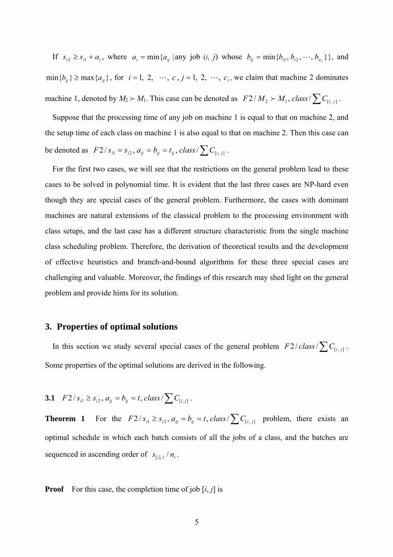
Proof For this case, the completion time of job [i, j] is

5

tjnsCi

kk

i

kkji )1(

1

111],[],[ +++= ∑∑

−

==

.

The total flowtime is

.)()(

)]()([

)(

])1([

1 11],[

11],[1],1[1],2[1],1[21],1[1

1 11 11 11],[

1

1

111],[

1

1 1],[

11

11

∑ ∑ ∑

∑

∑∑∑ ∑∑ ∑

∑ ∑∑∑

∑∑

= = =

=

= ==

+++

+++== =

=

−

===

= =

++=

++++++++=

++=

+++=

=

−

−

r

i

r

ik

n

jki

n

jrr

r

i

n

j

r

i

nnn

nnj

r

i

i

kki

r

i

i

kk

i

kk

n

j

r

i

n

jji

tnjns

ntjtssnssnsn

tjtsn

tjns

CF

iii

i

i

i

LL

L

L

i) For all schedules that consist of r batches, if a schedule satisfies

, then it has the smallest value of the total flowtime.

21],2[11],1[ // nsns ≤

rr ns /1],[≤≤L

Let σ1 denote a schedule where the batches are sequenced by

, and σrr nsnsns /// 1],[21],2[11],1[ ≤≤≤ L 2 denote a schedule that is obtained from σ1 by

interchanging the batches only in positions i and i+k . Denoting the total flowtime of σ)1( ≥k 1

and σ2 as F(σ1) and F(σ2), respectively, we have

.)()()(

)([)(

),()(

1],[1

1],1[1],[1

1],1[

11],1[1],[

11],1[

11],1[

12

1],[1

1],1[1

1

∑∑∑∑

∑∑∑∑∑

∑∑∑

=++=+++

+=+

−+=−+

++=

+=

+−=

−==

===

+++−++−++

+−+++++++=

++++=

r

rjjr

r

kijjkikii

r

kijjikii

r

kijjki

kii

r

ijji

r

ijjki

r

ijji

r

jj

n

j

r

rjjr

r

jj

n

j

nsnsnnnsnnns

nnnsnsnsnsjtntF

nsnsjtntF

L

LL

L

σ

σ

Then,

),()]()([

)]()([

)()(

))(())(()()(

1],[1],[1],1[1],1[111],[

111],[1],1[1],1[

11],[11],[

1],1[1],1[1],[1],[12

kiiikikiikikiiki

kiiikiii

rkikikirkiii

kiikiirkiiiki

nsnsssnnns

nnsssn

nnnsnnns

ssnnnnnssFF

++−+++−+++

−++−++

++++++

−+++++

−+++−+++

++−++=

+++−++++

++−+++++−=−

LL

LL

LL

LLL

σσ

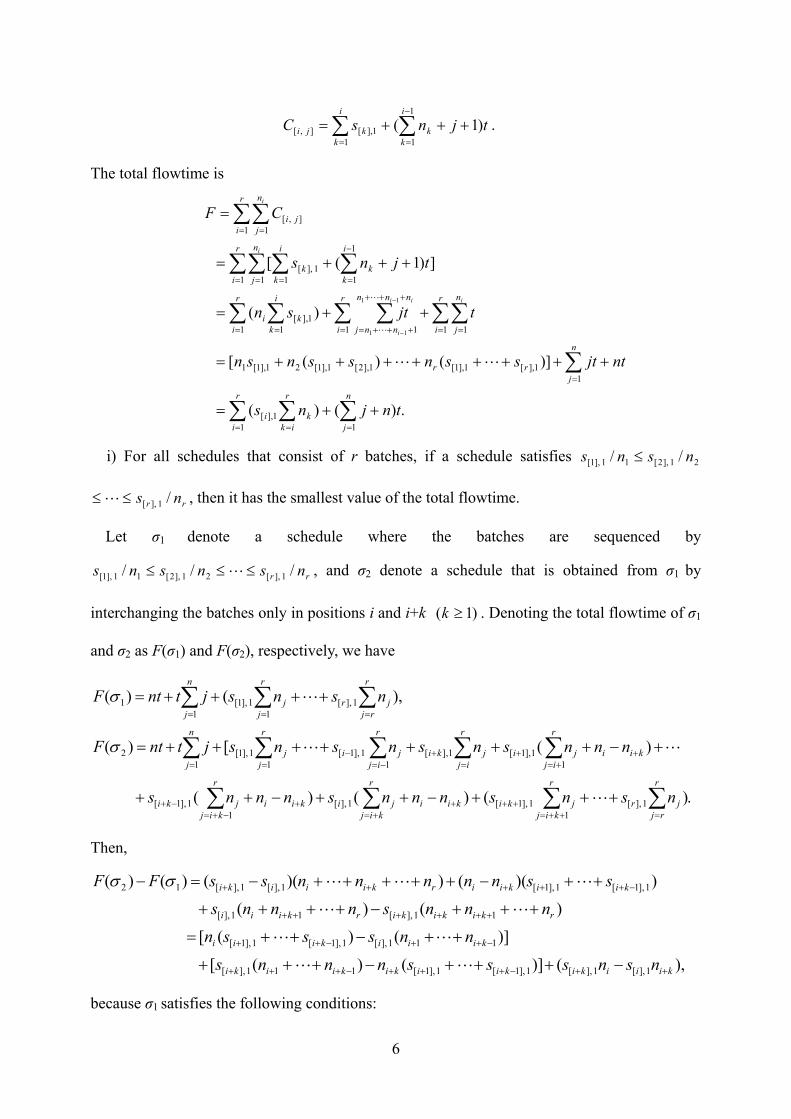
because σ1 satisfies the following conditions:

6

, rr nsnsns /// 1],[21],2[11],1[ ≤≤≤ L

we have

.

),()(

),()(

1],[1],[

1],1[1],1[111],[

111],[1],1[1],1[

kiiiki

kiikikiiki

kiiikiii

nsns

ssnnns

nnsssn

++

−+++−+++

−++−++

≥

++≥++

++≥++

LL

LL

Therefore, 0)()( 12 ≥− σσ FF .

ii) Given a schedule (denoted as σ1) in which the batches are sequenced in ascending order

of , if the kth and lth batches (k + 1 < l) belong to the same job class, then we merge

the two batches and again sequence all batches in ascending order of . The total

flowtime of the resulting schedule (denoted as σ

ii ns /1],[

ii ns /1],[

2) is less than that of the original schedule σ1.

We assume that the merged batch is in the ith position of schedule σ2. Obviously, ki ≤

because kklkk nsnns /)/( 1],[1],[ <+ . We have

)()( 1],[1

1],1[1

1 ∑∑∑===

++++=r

rjjr

r

jj

n

j

nsnsjtntF Lσ

and

.

)()()(

)()(

1],[1

1],1[

11],1[

11],1[

11],1[

1],[1],[1

1],1[1

1],1[1

2

∑∑

∑∑∑

∑∑∑∑∑

=+=+

−=−

+=+

−=−

==−=−

==

+++

−++−+−−++

−−++++++=

r

rjjr

r

ljjl

l

r

ljjll

r

kjjklk

r

kjjk

lk

r

ijji

r

ijjk

r

ijji

r

jj

n

j

nsns

nnsnnsnnns

nnnsnsnsnsjtntF

L

LL

L

σ

Then,

).(

)())(()()()(

111],[

1],1[1],1[1],1[1],[1],[21

−+

−+−

+++−

+++++++++=−

kiik

llklkkirll

nnns

nssnnssnnsFF

L

LLL

σσ

Note that schedule σ2 satisfies the following condition:

.///)/( 11],1[11],1[1],[1],[ −−++ ≤≤≤≤+ kkiiiilkk nsnsnsnns L

So, we have

))(()( 1],1[1],1[1],[111],[ lkkiikiik nnsssnnns ++++≤+++ −+−+ LL .

7

Therefore, F(σ1) − F(σ2) > 0.

From i) and ii), we reach the conclusion of the theorem. □

According to Theorem 1, an algorithm that treats a job class as a single batch and sequences

the batches in ascending order of produces an optimal solution. ii ns /1],[

3.2 ∑==≤+ ],[21 /,,/2 jiijijii CclasstbastsF .

Theorem 2 For the ∑==≤+ ],[21 /,,/2 jiijijii CclasstbastsF problem, an optimal

schedule can be obtained if a batch consists of all the jobs of a class, and the batches are

sequenced in ascending order of . ii ns /2],[

Proof Similar to the proof of Theorem 1. □

According to Theorem 2, an algorithm that treats a job class as a single batch and sequences

all batches in ascending order of produces an optimal solution. ii ns /2],[

3.3 . ∑ ],[21 /,/2 jiCclassMMF f

Theorem 3 For the ∑ ],[21 /,/2 jiCclassMMF f problem, there exists an optimal

schedule where the jobs in a batch i are sequenced in ascending order of . ],[ jia

Proof Let σ1 denote a schedule that comprises r batches. Let σ2 denote a schedule obtained

by interchanging only the jobs [i, j] and [i, j+k] in schedule σ)1( ≥k 1. Obviously, the

completion times of the jobs up to job [i, j–1] or after job [i, j+k] in the same positions of σ1

and σ2 are equal. In schedule σ1, we have

,)( ],[1

],[

1

1 1],[

11],[],[1 ji

j

qqi

i

p

n

qqp

i

ppji baasC

p

+++= ∑∑∑∑=

−

= ==

σ

8

],[1

],[

1

1 1],[

11],[],[1 )( hji

hj

qqi

i

p

n

qqp

i

pphji baasC

p

+

+

=

−

= ==+ +++= ∑∑∑∑σ , for .,,2,1 kh L=

In schedule σ2, we have

],[],[

1

1],[

1

1 1],[

11],[],[2 )( kjikji

j

qqi

i

p

n

qqp

i

ppji baaasC

p

++

−

=

−

= ==

++++= ∑∑∑∑σ ,

],[1

],[],[

1

1],[

1

1 1],[

11],[],[2 )( hji

hj

jqqikji

j

qqi

i

p

n

qqp

i

pphji baaaasC

p

+

+

+=+

−

=

−

= ==+ +++++= ∑∑∑∑∑σ , for 1,,2,1 −= kh L ,

.)( ],[1

],[

1

1 1],[

11],[],[2 ji

kj

qqi

i

p

n

qqp

i

ppkji baasC

p

∑∑∑∑+

=

−

= ==+ +++=σ

Then

)()()( ],[],[],[1],[2 jikji

ki

jqqi

kj

jqqi aakCC −+= +

+

=

+

=∑∑ σσ .

If , then the total flowtime F(σ],[],[ kjiji aa +≤ 1) and F(σ2) of schedules σ1 and σ2, respectively,

have the following relation

∑∑∑∑= == =

=≤=r

p

n

qqp

r

p

n

qqp

pp

CFCF1 1

],[221 1

],[11 )()()()( σσσσ .

Hence, schedule σ1 is no worse than schedule σ2. □


schedule where the batches are sequenced in ascending order of . i

n

jjii nas

i

/)(1

],[1],[ ∑=

+

Proof In the ith batch, we have

],[1

],[

1

1 1],[

11],[],[ ji

j

lli

i

k

n

llk

i

llji baasC

k

+++= ∑∑∑∑=

−

= ==

, for inj ,,2,1 L= ,

.)1(1

],[],[1

1

1 1],[

11],[

1],[ ∑∑∑∑∑∑

==

−

= ===

++−++=iiki n

llili

n

li

i

k

n

llki

i

lli

n

jji balnansnC

In the (i+1)st batch, we have

9

∑∑∑∑∑∑+++

=++

=+

= =+

+

=+

=+ ++−++=

111

1],1[],1[

11

1 1],[1

1

11],[1

1],1[ )1(

iiki n

llili

n

li

i

k

n

llki

i

lli

n

jji balnansnC .

Then

.)1()1(

)()()(

11

1

1],1[

1],[],1[

11],[

11],[1

1],1[11],[1

1

1 1],[1

1

11],[1

1],1[

1],[

∑∑∑∑∑

∑∑∑∑∑++

+

=+

=+

=+

==+

+++

−

= =+

−

=+

=+

=

+++−++−++

++++++=+

iiiii

kii

n

lli

n

llili

n

lili

n

li

n

llii

iiiii

i

k

n

llkii

i

llii

n

jji

n

jji

bbalnalnan

snsnnannsnnCC

Interchanging the ith and (i+1)st batches, the sum of the job completion times within the two

batches is

.)1()1(

)()()(

1],[

1],1[],[

1],1[

11

1],1[

1],[1],1[1

1

1 1],[1

1

11],[1

1],1[

1],[

111

1

∑∑∑∑∑

∑∑∑∑∑

==+

=+

=+

=+

++

−

= =+

−

=+

=+

=

+++−++−++

++++++=′+′

+++

+

iiiii

kii

n

lli

n

llili

n

lili

n

li

n

jjii

iiiii

i

k

n

llkii

i

llii

n

jji

n

jji

bbalnalnan

snsnnannsnnCC

Clearly, the completion times of the jobs before the ith batch or after the (i+1)st batch are not

changed after interchanging the ith and (i+1)st batches. Then, for the total completion time F

and F′ before and after interchanging, respectively, we have

).()(

)()(

1

11

1],1[1],1[

1],[1],[1

1],1[

1],[

1],1[

1],[

∑∑

∑∑∑∑+

++

=++

=+

=+

==+

=

+−+=

′+′−+=′−

ii

iiii

n

jjiii

n

jjiii

n

jji

n

jji

n

jji

n

jji

asnasn

CCCCFF

If , we have 11

],1[1],1[1

],[1],[ /)(/)(1

+=

++=

∑∑+

+≤+ i

n

jjiii

n

jjii nasnas

ii

0≤′− FF . □

Theorem 5 For the ∑ ],[21 /,/2 jiCclassMMF f problem, where the jobs in the ith and

(i+k)th batches belong to the same job class, there exists an optimal schedule where ] and

satisfy the following condition

,[ inia

]1,[ kia +

]1,[

1

1

1

1 1],[

11],[],[ /)( ki

k

lli

k

l

n

jjli

k

llini anasa

li

i +

−

=+

−

= =+

=+ ≤+≤ ∑∑∑∑

+

. (1)

Proof. In a schedule S, we denote all the processed jobs between job [i, ni] and job [i+k, 1] as

a partial sequence σ. Let S′ be the sequence formed by moving job [i+k, 1] to the last of the ith

10

batch in S. Clearly, the completion times of the jobs sequenced before job [i, ni] or after job

[i+k, 1] are not changed. Let F and F′ denote the total flowtime of S and S′, respectively. In

schedule S, we have

],[1

],[

1

1 1],[

11],[],[ jli

j

ggli

li

h

n

ggh

li

hhjli baasC

h

+=

+

−+

= =

+

=+ +++= ∑∑∑∑ , for ,,,2,1,1,,2,1 linjkl +=−= LL

.]1,[]1,[

1

1 1],[

11],[]1,[ kiki

ki

h

n

ggh

ki

hhki baasC

h

++

−+

= =

+

=+ +++= ∑ ∑∑

In schedule S′, we have

.,,2,1,1,,2,1for

),(

]1,[],[],[

11],[

1

1 1],[]1,[

]1,[]1,[1 1

],[1

1],[]1,[

likijlijli

k

hhi

k

h

n

jjhiki

kiki

i

h

n

jjh

i

hhni

njklaCC

saC

baasC

hi

h

i

++++

=+

−

= =++

++= ==

+

=−=+=′

+−=

+++=′

∑∑∑

∑∑∑+

LL ,

Then,

)(1

1 1],[

11],[]1,[

1

1]1,[

1

1 1],[]1,[

1

1 1],[ ∑∑∑∑∑∑∑∑

−

= =+

=++

−

=++

−

= =++

−

= =+

+++

+−++=′+′k

h

n

jjhi

k

hhiki

k

lliki

k

l

n

jjlini

k

l

n

jjli

hili

i

li

asCnaCCC .

Therefore,

)(1

1 1],[

11],[

1

1]1,[ ∑∑∑∑

−

= =+

=+

−

=++

+

+−=−′k

h

n

jjhi

k

hhi

k

lliki

hi

asnaFF .

Therefore, if the right hand side of inequality (1) holds, i.e., F′– F ≥ 0, which means that job

[i+k ,1] should not be moved to the last position of the ith batch to minimize the total flowtime.

Similar to the above, we can also prove that if the left hand side of inequality (1) holds, job [i,

ni] should not be moved to the beginning position of the (i+k)th batch to minimize the total

flowtime. □

3.4 . ∑ ],[12 /,/2 jiCclassMMF f


schedule where the jobs in a batch i are sequenced in ascending order of . ],[ jib

11



schedule where the batches are sequenced in ascending order of . i

n

jjii nbs

i

/)(1

],[2],[ ∑=

+


Theorem 8 For the ∑ ],[12 /,/2 jiCclassMMF f problem, where the jobs of the ith and

(i+k)th batches belong to the same job class, there exists an optimal schedule where and

satisfy the following condition

],[ inib

]1,[ kib +

∑ ∑∑∑−

=+

−

=+

=+

=+ ≤+≤

+1

1]1,[

1

11],[

12],[],[ /)(

k

lki

k

lli

n

jjli

k

llini bnbsb

li

i.


3.5 ∑=== ],[21 /,,/2 jiijijijii CclasstbassF .

For convenience, we set si1 = si2 = si, for ,,,2,1 ci L= and ai j = bi j= ti j, for

. For this special case, we can derive some optimal properties in the following.

,1=i ,,,2 cL

icj ,,2,1 L=

Theorem 9 For the ∑=== ],[21 /,,/2 jiijijijii CclasstbassF problem, there exists an

optimal schedule where the jobs in a batch i are sequenced in ascending order of . ],[ jit

Proof Let σ1 denote a sequence where the jobs within a batch are sequenced in ascending

order of t[i, j]. Let σ2 denote a sequence that is obtained from σ1 by swapping the jobs [i, j] and [i,

j+1]. Obviously, the completion times of all jobs before job [i, j] are equal in σ1 and σ2. In

schedule σ1, we have

12

,},max{)( ],[]1,[],[1,],[1 jijijijiji tCtAC ++= −−σ

]1,[],[1]1,[],[1,]1,[1 })(,max{)( ++−+ +++= jijijijijiji tCttAC σσ

]1,[],[]1,[],[1,]1,[1, },,max{ +−−+− ++++= jijijijijijiji ttCtAtA

,},max{ ]1,[],[]1,[]1,[1, +−+− +++= jijijijiji ttCtA (2)

},max{)()( ]1,[],[1,]1,[1],[1 −−+ +=+ jijijijiji CtACC σσ

.2},max{ ]1,[],[]1,[]1,[1, +−+− ++++ jijijijiji ttCtA (3)


,},max{)( ]1,[]1,[]1,[1,],[2 +−+− ++= jijijijiji tCtAC σ

],[],[2],[]1,[1,]1,[2 })(,max{)( jijijijijiji tCttAC +++= +−+ σσ

]1,[],[]1,[]1,[1,],[1, },,max{ +−+−− ++++= jijijijijijiji ttCtAtA

,},max{ ]1,[],[]1,[]1,[1, +−+− +++= jijijijiji ttCtA (4)

.2},max{2)()( ]1,[],[]1,[]1,[1,]1,[2],[2 +−+−+ +++=+ jijijijijijiji ttCtACC σσ (5)

From (2) and (4), we have ]1,[2]1,[1 )()( ++ = jiji CC σσ . And, obviously, swapping job [i, j] and

job [i, j+1] will not change the completion time of the last of these two jobs on machine 1. So

the completion times of all jobs after job [i, j+1] in σ1 are not changed in σ2. From (3) and (5),

we have

]1,[2],[2]1,[1],[1 )()()()( ++ +≤+ jijijiji CCCC σσσσ .

Then, the total flowtime of σ1 is no greater than the total flowtime of σ2. □

Theorem 10 For the ∑=== ],[21 /,,/2 jiijijijii CclasstbassF problem, in a sequence where

batches i and k are adjacent, let the jobs within batch i (or k) be sequenced in ascending order

of their processing times on machine 1 or 2. In order to minimize the total flowtime, batch i

should precede batch k, if

1kin tti≤ and . (6) k

n

jkjki

n

jiji ntsnts

ki

/)(/)(11∑∑==

+≤+

13

Proof We assume that batches i and k are in positions h and h+1 in a sequence σ1,

respectively, and sequence σ2 is obtained by swapping batches i and k. Obviously, the

completion times of any job before the hth batch are equal in σ1 and σ2. For the hth and (h+1)st

batches in sequence σ1, we have

ijjiiinhijiinhjh tttsCttsAChh

+++++++++= −−− −−},max{)( 1,1],1[1,1],[1 11

LLσ

,},max{)( ],1[,11

11

−− −−=

+++= ∑ hh nhijnh

j

lili CtAts for ,,,2,1 inj L=

,},,max{)()(

)}(

,)(,)(max{)(

})(,max{)(

})(,max{)(

],1[,1,111

1],1[

1,1

1,1

1

],[1,1

1,1],[11,],1[1

111

1

11

−−−

−

−−

−−−==

=−

=−

=−

=

=

−+

++++++=

++

++++++++=

+++=

+++++++++=

∑∑

∑

∑∑∑

∑

hihh

i

i

h

i

i

h

i

h

ik

ih

nhinnhkjnh

j

lklk

n

lili

n

lilinh

in

n

lilinhkj

n

lilinh

j

lklk

nhkjnh

j

lklk

kjjkkknhkjkknhjh

CtAtAtsts

tsC

ttsAttsAts

CtAts

tttsCttsAC

σ

σσ LL

for (7) ,,,2,1 knj L=

∑∑∑∑===

+=

+−++++=+iiki n

lili

n

lilkkkiki

n

jjh

n

jjh tlntnsnsnnCC

111],1[1

1],[1 )1()()()( σσ

},{max)1( ],1[,111

11 −− −−==

+++−+ ∑∑ hh

ik

nhilnh

n

l

n

lklk CtAtln

. (8) },,{max ],1[,1,11

111 −−− −−−=

+++∑ hihh

k

nhinnhklnh

n

l

CtAtA

For the hth and (h+1)st batches in sequence σ2, similar to the above, we can derive

},,max{)()( ],1[,11

],[2 11 −− −−=

+++= ∑ hh nhkjnh

j

lklkjh CtAtsC σ for ,,,2,1 knj L=

}.,,max{)()()( ],1[,1,111

],1[2 111 −−− −−−==

+ ++++++= ∑∑ hkhh

k

nhknnhijnh

j

lili

n

lklkjh CtAtAtstsC σ

for inj ,,2,1 L= , (9)

14

∑ ∑

∑ ∑ ∑ ∑

= =−−

= = = =+

−−+++−+

+−++++=+

i k

hh

k i k k

n

l

n

lnhklnhili

kl

n

j

n

j

n

l

n

lkkliiikkijhjh

CtAtln

tlntnsnsnnCC

1 1],1[,1

1 1 1 1],1[2],[2

},max{)1(

)1()()()(

11

σσ

(10) .},,max{1

],1[,1,1 111∑=

−−− −−−+++

i

hkhh

n

lnhknnhilnh CtAtA

From (7) and (9), we have

],1[2],1[1 )()(ik nhnh CC ++ = σσ .

Then, the completion times of any job after the (h+1)st batch in σ1 and σ2 are equal.

From (6), (8) and (10), we have

∑ ∑ ∑∑= = =

++=

+≤+k i ki n

j

n

j

n

jjhjhjh

n

jjh CCCC

1 1 1],[2],1[2],1[1

1],[1 )()()()( σσσσ .

Thus, if the condition of the theorem holds, then the conclusion is valid. □

Theorem 11 For the ∑=== ],[21 /,,/2 jiijijijii CclasstbassF problem, jobs within any

batches are sequenced in ascending order of their processing times on machine 1 or 2, and the

jobs in the ith and (i+k)th batches belong to the same job class. In order to minimize the total

flowtime,

i) job [i+k, 1] should move to the last position of the ith batch, if , for

;

]1,[]1,[ liki tt ++ ≤

1,,2,1 −= kl L

ii) job should move to the first position of the (i+k)th batch, if , for

.

],[ ini ],[],[ lii nlini tt++≥

1,,2,1 −= kl L

Proof i) Let σ1 denote the original schedule, and σ2 a schedule obtained from σ1 by moving

the first job in the (i+k)th batch to the last position of the ith batch. Obviously, the completion

times of all the jobs from the first job up to job [i, ni] in σ1 and σ2 are equal. Under the

assumptions of the theorem, in schedule σ1, we have

15

},max{)( ],[],1[1

],1[]1[],1[1 ii nijini

j

lliiji CtAtsC +

=+++ +++= ∑σ , for ,,,2,1 1+= inj L

},,,,max{)( ],[],[],1[],1[],[1 11 iiliiii nijlininlinininijli CtAtAtAC +−+++ +++=−++

Lσ

∑∑∑∑=

+

−

= =+

=+ +++

+ j

hhli

l

h

n

jjhi

l

hhi tts

hi

1],[

1

1 1],[

1][ , for linjkl +== ,,2,1,,,2 LL . (11)


, },max{)( ]1,[],[]1,[]1,[2 kinikinini tCtACiii +++ ++=σ

]1,[],1[1],1[2 )()( kijiji tCC +++ += σσ , for ,,,2,1 1+= inj L

},,,,,max{)( ],[]1,[],[],1[],1[],[2 11 iiiliiii nikinijlininlinininijli CtAtAtAtAC ++−+++ ++++=−++

Lσ

,]1,[1

],[

1

1 1],[

1][ ki

j

hhli

l

h

n

jjhi

l

hhi ttts

hi

+=

+

−

= =+

=+ ++++ ∑∑∑∑

+

for ,,,2,1,1,,2 linjkl +=−= LL

},(max{)()()()( ],[]1,[

1

1 1],[1]1,[1

1

1 1],[2]1,[2 ii

lili

i nikini

k

l

n

jjliki

k

l

n

jjlini CtACCCC +

−

= =++

−

= =++ +++=+ ∑∑∑∑

++

σσσσ

}),,,,max{ ],[]1,[],1[],1[ 11 iikiiii nikininkininini CtAtAtA +−++ +++−−++

L

,)( 1

][

1

1 1],[

1

1]1,[ ∑∑∑∑

=+

−

= =+

−

=++ −−+

+ k

hhi

k

h

n

jjhi

k

lliki stnt

ih

(12)

},,,,,max{)( ],[]2,[],1[],1[]1,[]1,[2 11 iikiiiii nikininkinininikiniki CtAtAtAtAC +−++++ ++++=−++

Lσ

.]2,[]1,[

1

1 1],[

1][ kiki

k

h

n

jjhi

k

hhi ttts

hi

++

−

= =+

=+ ++++ ∑∑∑

+

(13)

From (11) and (13), considering that ]2,[]1,[ kiki tt ++ ≤ , we have ]1,[2]2,[1 )()( kiki CC ++ = σσ . So, the

completion times of all the jobs after job [i+k, 1] in schedule σ1 are the same as those in

schedule σ2.

Furthermore, from (12), taking into account that ]1,[]1,[ liki tt ++ ≤ , 1,,2,1 −= kl L , we have

∑∑∑∑−

= =++

−

= =++

++

+<+1

1 1],[1]1,[1

1

1 1],[2]1,[2 )()()()(

k

l

n

jjliki

k

l

n

jjlini

lili

iCCCC σσσσ .

Therefore, the total flowtime of σ2 is less than the total flowtime of σ1.

ii) Similar to the proof of i). □

16

4. Algorithms

In the previous section, we have derived some properties of the optimal solutions for several

special cases. Since Theorems 1 and 2 state the conditions for the optimal solutions for cases

3.1 and 3.2, respectively, it is easy to develop polynomial time solution algorithms for these

two cases. In this section, we develop some heuristics and branch-and-bound algorithms for

cases 3.3, 3.4 and 3.5.

4.1 Heuristic algorithms

Our heuristic algorithms use a construction procedure to find an initial schedule, and then

improve the performance of the solutions according to the optimal properties stated in the

various theorems in the previous section.

For , we construct the following algorithms. ∑ ],[21 /,/2 jiCclassMMF f

Heuristic algorithm A1(HAA1)

Step 1. Let )],(,),2,(),1,([ ii cijobijobijob L=σ be the sequence in ascending order of

their processing times on machine 1, ci ,,2,1 L= , and set Φ=β (empty set).

Step 2. Select a job (i, 1) such that },,2,1|min{ 1111 ckasas kkii L=+=+ . Remove job (i, 1)

from iσ and place it in the first position of β , and set h = i.

Step 3. If Φ=∪∪∪ cσσσ L21 , go to step 4, else

If Φ≠hσ and ikihm asa +≤ 1 , remove job (h, m) from hσ and place it in the last position

of β . Otherwise, remove job (i, k) from iσ and place it in the last position of β , and set h

= I, where job (h, m) is the first job in hσ , and job (i, k) satisfies si1 + aik = min{sg1+ ag l | job

(g, l) is the first job in gσ , }. Go to step 3. hg ≠

17

Step 4. For sequence β , calculate for its batches, and sequence all

batches of

i

n

jjii nas

i

/)(1

],[1],[ ∑=

+

β in ascending order of . i

n

jjii nas

i

/)(1

],[1],[ ∑=

+

Step 5. For the two batches containing the jobs of the same class, move their jobs that satisfy

the conditions for the optimal solution given in Theorem 5. Denote the obtained sequence as β .

Step 6. Repeat step 4 if necessary. Stop.

Heuristic algorithm A2 (HAA2)

This heuristic is similar to HAA1 except step 3. We rewrite step 3 as follows.


If Φ≠hσ and ikimhhm asaa +≤+ + 11, 2/)( , remove jobs (h, m) and (h, m+1) from hσ and

place them in the last two positions of β . Otherwise, remove job (i, k) from iσ and place it

in the last position of β , and set h = I, where jobs (h, m) and (h, m+1) are the first two jobs in

hσ , and job (i, k) satisfies si1 + aik = min{sg1+ ag l | job (g, l) is the first job in gσ , }. Go

to step 3.

hg ≠

For , we have the following algorithms. ∑ ],[12 /,/2 jiCclassMMF f

Heuristic algorithm B1 (HAB1)

Step 1. Let )],(,),2,(),1,([ ii cijobijobijob L=σ be the sequence in ascending order of

their processing times on machine 2, ci ,,2,1 L= , and set Φ=β .

Step 2. Select a job (i, 1) such that },,2,1|min{ 1212 ckbsbs kkii L=+=+ . Remove job (i,

1) from iσ and place it in the first position of β , and set h = i.


18

If Φ≠hσ and ikihm bsb +≤ 2 , remove job (h, m) from hσ and place it in the last position

of β . Otherwise, remove job (i, k) from iσ and place it in the last position of β , and set h

= I, where job (h, m) is the first job in hσ , and job (i, k) satisfies si2 + bik = min{sg2+ bg l | job (g,

l) is the first job in gσ , }. Go to step 3. hg ≠

Step 4. For sequence β , calculate for its batches, and sequence all

batches of

i

n

jjii nbs

i

/)(1

],[2],[ ∑=

+

β in ascending order of . i

n

jjii nbs

i

/)(1

],[2],[ ∑=

+

Step 5. For the two batches containing jobs of the same class, move their jobs that satisfy the

conditions for the optimal solution given in Theorem 8. Denote the obtained sequence as β .

Step 6. Repeat step 4 if necessary. Stop.

Heuristic algorithm B2 (HAB2)

This heuristic is similar to HAB1 except step 3. We rewrite step 3 as follows.


If Φ≠hσ and ikimhhm bsbb +≤+ + 21, 2/)( , remove jobs (h, m) and (h, m+1) from hσ and



hσ , and job (i, k) satisfies si2 + bik = min{sg2+ bg l | job (g, l) is the first job in gσ , }. Go

to step 3.

hg ≠

For ∑=== ],[21 /,,/2 jiijijijii CclasstbassF , we construct the following algorithms.

Heuristic algorithm C1 (HAC1)

Step 1. Let )],(,),2,(),1,([ ii cijobijobijob L=σ be a sequence in ascending order of

19

their processing times on machine 1 or 2, ci ,,2,1 L= , and set Φ=β .

Step 2. Select a job (i, 1) such that },,2,1|min{ 11 cktsts kkii L=+=+ . Remove job (i, 1)

from iσ and place it in the first position of β , and set h = i.


If Φ≠hσ and , remove job (h, m) from ikihm tst +≤ hσ and place it in the last position of

β . Otherwise, remove job (i, k) from iσ and place it in the last position of β , and set h = I,

where job (h, m) is the first job in hσ , and job (i, k) satisfies si + tik = min{sg+ tg l | job (g, l) is

the first job in gσ , }. Go to step 3. hg ≠

Step 4. For sequence β , interchange the adjacent pairs of batches to improve the objective

function.

Step 5. For the two batches containing jobs of the same class, move their jobs that satisfy the

conditions for the optimal solution given in Theorem 11. Stop.

Heuristic algorithm C2 (HAC2)

This heuristic is similar to HAC1 except step 3. We rewrite step 3 as follows.


If Φ≠hσ and (thm + th, m+1) / 2 ≤ si + tik , remove jobs (h, m) and (h, m+1) from hσ and



hσ , and job (i, k) satisfies si + tik = min{sg+ tg l | job (g, l) is the first job in gσ , }. Go to

step 3.

hg ≠

4.2 Branch-and-bound algorithms

For each of the above cases, we derive a lower bound that can be used to reduce the size of

the search tree generated by the branch-and-bound procedure.

20

We assume that a partial sequence σ1 has been determined, in which job (p, q) is the last job,

and σ2 is the complement of σ1, which include α unscheduled jobs.

For case 3.3, in set σ2, let denote the processing time of job (i, j) on

machine 1, where job (i, j) is the kth job when being sequenced among these

),,2,1( αL=kakij

α jobs in

increasing order of their processing times on machine 1. Let nil > 0 ( β,,2,1 L=l ) denote the

job number of class i in σ2 (excluding class p), where l denotes the lth position in increasing

order of sli 1 / ni

l, and sil1 denotes the setup time of these nl

i jobs on machine 1. A lower bound

for the case 3.3 can be expressed as follows:

∑∑ ∑∑∑∈∈ ===

++−+−++=21 ),(),( 1

11

)1()()(1σσ

αββ

ααji

ijkij

ji kpqpq

lk

ki

li

lij bakbCnsCLB . (14)


machine 2, where job (i, j) is the kth job when being sequenced among these

),,2,1( αL=kbkij

α jobs in

increasing order of their processing times on machine 2. Let nil >0 ( β,,2,1 L=l ) denote the

job number of class i in σ2 (excluding class p), where l denotes the lth position in increasing

order of sil2 / ni

l and sil2 denotes the setup time of these ni

l jobs on machine 2. A lower bound for

the case 3.4 can be expressed as follows:

kij

ji kpq

lk

ki

li

lij bkCnsCLB ∑ ∑∑∑

∈ ===

+−+++=1),( 1

21

)1()(2σ

αββ

αα . (15)


machine 1 or 2, where job (i, j) is the kth job when being sequenced among these

),,2,1( αL=kt kij

α jobs in

increasing order of their processing times on machine 1 or 2. Let nil >0 ( β,,2,1 L=l ) denote

the job number of class i in σ2 (excluding class p), where l denotes the lth position in increasing

order of si / nil and si

l denotes the setup time of these nil jobs on machine 1 or 2. A lower bound

for the case 3.5 can be expressed as follows:

}.0,{max)1()(31),( 111

pqkijpq

ji k

kij

kpq

lk

ki

l

liij CtAtkCnsCLB −+++−+++= ∑ ∑∑∑∑

∈ ====σ

ααββ

αα (16)

The branch-and-bound algorithm for case 3.3 can be described as follows: At the root node

of the branch-and-bound search tree, the best result generated by HAA1 and HAA2 is applied

21

as an initial upper bound. At each node of the branch-and-bound search tree, the optimal

properties of Theorems 3 to 5 are used as pruning devices, and if the current lower bound is

greater than the upper bound, this node is pruned.


of the branch-and-bound search tree, the best result generated by HAB1 and HAB2 is applied





of the branch-and-bound search tree, the best result generated by HAC1 and HAC2 is applied




5. Computational results

The measures of the effectiveness of the heuristic algorithms are the average relative error

and maximal relative error from the optimal total flowtime, where the relative error is defined

as: relative error (%) = [(heuristic total flowtime – optimal total flowtime) x 100]/[optimal total

flowtime]. The branch-and-bound algorithms are evaluated with respect to the average CPU

time in seconds and the average number of nodes searched. The procedures were coded in VB

5.0 and run on a Celeron 300 PC.

Fifty random instances were generated for each of feasible combinations of n = 20, 30 jobs

and different numbers of job classes. The job processing times for case 3.3 on machines 1 and

2 were uniformly distributed integers between 50 and 100 and between 1 and 50, respectively.

The job processing times for case 3.4 on machines 1 and 2 were uniformly distributed integers

between 1 and 50, and between 50 and 100, respectively. The job processing times for case 3.5

were uniformly distributed integers between 1 and 100. The class setup times for case 3.3 on

machine 1, and case 3.5 on machines 1 and 2 were uniformly distributed integers between 1

and 100. The class setup times for case 3.4 on machine 2 were uniformly distributed integers

22

between 50 and 100. The class setup times for case 3.3 on machine 2, and for case 3.4 on

machine 1 were randomly generated integers according to the definitions of cases 3.3 and 3.4,

respectively. We present a summary of our findings in Tables 1, 2 and 3.

Table 1 reports the performance of HAA1 and HAA2 of case 3.3. It is obvious that HAA1 is

better than HAA2 except that for 30 jobs divided into 3 classes. We notice that the flowtime is

made up of the job processing times and the job class setups. In general, the optimal objective

is obtained through balancing these two items. Since HAA2 tends to produce more batches

than HAA1, HAA2 is more likely to produce a better solution for the scheduling problem with

fewer job classes. It seems that the mean relative errors for the two heuristics are independent

of the number of jobs. The mean relative error for HAA1 decreases as the number of class

decreases.

Table 1 also reveals that the branch-and-bound algorithm can find the optimal solutions for

all the problems generated. Both the searched nodes and CPU time tend to decrease as the

number of classes increases, which is indicated by the expression of the lower bound (14) as

the more the jobs are divided into job classes, the tighter the lower bound becomes.

Table 2 reports the performance of HAB1 and HAB2 and the branch-and-bound algorithm

for case 3.4, and Table 3 the performance of HAC1 and HAC2 and the branch-and-bound

algorithm for case 3.5. The algorithms for cases 3.4 and 3.5 have similar characters as those of

the algorithms for case 3.3.

Since the conditions for the optimal solution for case 3.5 are stricter than those for cases 3.3

and 3.4, it is evident that the branch-and-bound algorithm for case 3.5 searches more nodes and

requires more CPU time than those for cases 3.3 and 3.4.

6. Conclusions

In this paper we have considered several special cases of the two-machine flowshop

scheduling with job class setups and derived some optimal solution properties for these

problems to minimize the total flowtime. We have discussed the use of these optimal properties

to develop heuristic algorithms. We have also developed branch-and-bound algorithms for

cases 3.3, 3.4 and 3.5, in which the best solution of two heuristic algorithms is used as an initial

23

upper bound, and the derived lower bounds and optimal properties are used to reduce the size

of the search tree. We have conducted computational experiments to test these algorithms and

the results demonstrate that all of the algorithms are very efficient and effective in solving the

special cases under study.

Acknowledgements

This research was supported in part by The Hong Kong Polytechnic University under a grant

from the Area of Strategic Development in China Business Services. We are grateful to two

anonymous referees for their helpful comments on an earlier version of this paper.

References

B.-H. Ahn and J.-H. Hyun, “Single facility multi-class job scheduling”, Computers &

Operations Research, 1990, 17, 265-272.

A. Allahverdi, “Minimizing mean flowtime in a two-machine flowshop with sequence

independent setup times”, Computers & Operations Research, 2000, 27, 111-127.

P. Brucker, Scheduling Algorithms, Spring-Verlag, Berlin, 1995.

T.C.E. Cheng, J.N.D. Gupta and G.Q. Wang, “A review of flowshop scheduling with setup

times”, Production and Operations Management, 2000, 9, 262-282.

H.A.J. Crauwels, A.M.A. Hariri, C.N. Potts and L.N. Van Wassenhove, “Branch and bound

algorithms for single-machine scheduling with batch set-up times to minimize total

weighted completion time”, Annals of Operations Research, 1998, 83, 59-76.

H.A.J. Crauwels, C.N. Potts and L.N. Van Wassenhove, “Local search heuristics for single

machine scheduling with batch set-up times to minimize total weighted completion

time”, Annals of Operations Research, 1997, 70, 261-279.

T. Gonzalez and S. Sahni, “Flowshop and job shop schedules: complexity and approximation”,


J.N.D. Gupta, “Optimal schedules for single facility with two job classes”, Computers &


J.N.D. Gupta, “Single facility scheduling with multiple job classes”, European Journal of

24

Operational Research, 1988, 8, 42-45.

J.C. Ho and J.N.D. Gupta, “Flowshop scheduling with dominant machines”, Computers &


A.J. Mason and E.J. Anderson, “Minimizing flow time on a single machine with job classes

and setup times”, Naval Research Logistics, 1991, 38, 333-350.

C.N. Potts, “Scheduling two job classes on a single machine”, Computers & Operations

Research, 1991, 18, 411-415.

C.N. Potts and M.Y. Kovalyov, “Scheduling with batching: a review”, European Journal of

Operational Research, 2000, 120, 228-249.

C.N. Potts and L.N. Van Wassenhove, “Integrating scheduling with batching and lot-sizing: a

review of algorithms and complexity”, Journal of the Operational Research Society,

1992, 43, 395-406.

S. Webster and K.R. Baker, “Scheduling groups of jobs on a single machine”, Operations

Research, 1995, 43, 692-704.

H.-S. Woo and D.-S. Yim, “A heuristic algorithm for mean flowtime objective in flowshop

scheduling”, Computers & Operations Research, 1998, 25, 175-182.

25

Table 1. Performance evaluation of HAA1, HAA2 and the branch-and-bound algorithm.

HAA1 HAA2 Branch-and-bound No. of jobs

No. of classes Mean(%) Max(%) Mean(%) Max(%) Nodes Times

20 2 0.050 0.573 0.092 0.869 4179 25.95 4 0.000 0.000 0.046 0.919 968 5.97 5 0.000 0.000 0.000 0.000 30 0.22 10 0.000 0.000 0.000 0.000 17 0.284

30 3 0.838 3.426 0.497 3.426 65945 1181.52 5 0.017 0.330 0.060 0.129 2646 44.658 6 0.000 0.000 0.284 4.947 37 0.759 10 0.006 0.366 0.024 0.146 29 0.832

Table 2. Performance evaluation of HAB1, HAB2 and the branch-and-bound algorithm.

HAB1 HAB2 Branch-and-bound No. of

jobs No. of classes Mean(%) Max(%) Mean(%) Max(%) Nodes Times

20 2 0.923 3.766 0.922 3.716 5614 36.227 4 0.499 4.428 0.055 4.428 3481 19.538 5 0.000 0.000 0.002 0.045 37 0.2265 10 0.000 0.000 0.000 0.000 18 0.291

30 3 0.941 2.137 0.542 4.221 58723 1102.12 5 0.018 0.356 0.044 0.701 9675 130.06 6 0.004 0.078 0.948 6.221 613 8.192 10 0.000 0.000 0.018 0.066 30 0.789

Table 3. Performance evaluation of HAC1, HAC2 and the branch-and-bound algorithm.

HAC1 HAC2 Branch-and-bound No. of jobs

No. of classes Mean(%) Max(%) Mean(%) Max(%) Nodes Times

20 2 0.947 1.392 0.787 1.351 7042 57.45 4 0.108 2.153 0.985 9.038 5433 44.45 5 0.066 1.257 1.351 6.761 228 1.6185 10 0.000 0.000 0.000 0.000 117 0.897

30 3 1.796 3.969 1.395 3.462 96536 1326.70 5 0.534 4.900 0.476 2.980 14759 443.45 6 0.000 0.000 0.532 1.432 110 2.861 10 0.048 0.894 1.669 5.339 89 0.914

26

Documents

Two-machine Flowshop Scheduling - Hong Kong …ira.lib.polyu.edu.hk/bitstream/10397/1153/1/(Revised... · · 2018-03-26Two-machine Flowshop Scheduling . ... developed a branch-and-bound