Introduction to Magnetic Resonance Imaging

Howard Halpern

Basic Interaction

• Magnetic Moment m (let bold indicate vectors)

• Magnetic Field B• Energy of interaction:

– E = -µ∙B = -µB cos(θ)

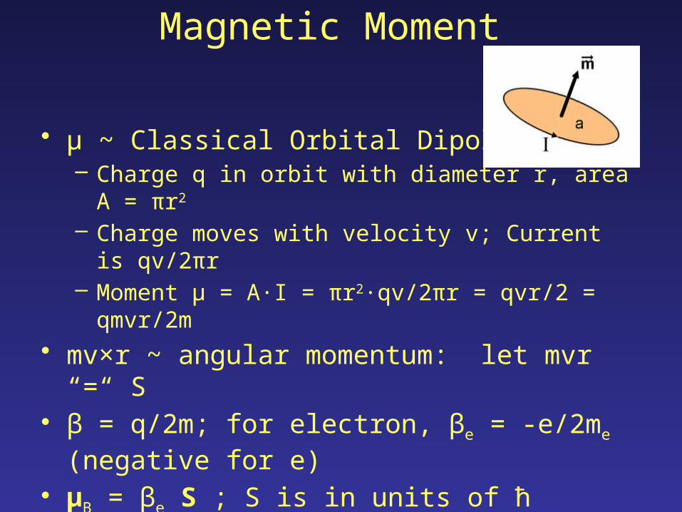
Magnetic Moment

• μ ~ Classical Orbital Dipole Moment– Charge q in orbit with diameter r, area A = πr2

– Charge moves with velocity v; Current is qv/2πr– Moment µ = A∙I = πr2∙qv/2πr = qvr/2 = qmvr/2m

• mv×r ~ angular momentum: let mvr “=“ S• β = q/2m; for electron, βe = -e/2me (negative for e)

• µB = βe S ; S is in units of ħ

–Key 1/m relationship between µ and m• µB (the electron Bohr Magneton) = -9.27 10-24 J/T

• µP (the proton Bohr Magneton) = 5.05 10-27 J/T****

Magnitude of the Dipole Moments

• Key relationship: |µ| ~ 1/m• Source of principle difference between

– EPR experiment– NMR experiment

• This is why EPR can be done with cheap electromagnets and magnetic fields ~ 10mT not requiring superconducting magnets

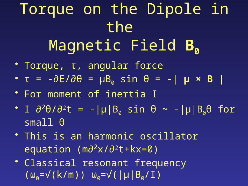
Torque on the Dipole in the Magnetic Field B0

• Torque, τ, angular force• τ = -∂E/∂θ = µB0 sin θ = -| µ × B |

• For moment of inertia I

• I ∂2θ/∂2t = -|µ|B0 sin θ ~ -|µ|B0θ for small θ

• This is an harmonic oscillator equation (m∂2x/∂2t+kx=0)

• Classical resonant frequency (ω0=√(k/m)) ω0=√(|µ|B0/I)

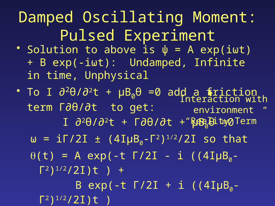
Damped Oscillating Moment: Pulsed Experiment

• Solution to above is ψ = A exp(iωt) + B exp(-iωt): Undamped, Infinite in time, Unphysical

• To I ∂2θ/∂2t + µB0θ =0 add a friction term Γ∂θ/∂t to

get:

I ∂2θ/∂2t + Γ∂θ/∂t + µB0θ =0

ω = iΓ/2I ± (4IµB0-Γ2)1/2/2I so that

(t) = A exp(-t Γ/2I - i ((4IµB0-Γ2)1/2/2I)t ) +

B exp(-t Γ/2I + i ((4IµB0-Γ2)1/2/2I)t )

Lifetime: T ~ 2I/ Γ

Redfield Theory: Γ~µ2 so T1s &T2s α 1/μ2

Interaction with environment

“Reality Term”

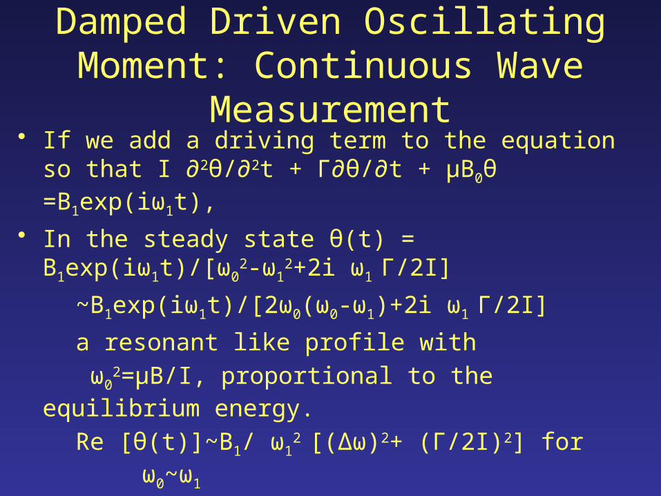
Damped Driven Oscillating Moment: Continuous Wave Measurement

• If we add a driving term to the equation so that I ∂2θ/∂2t + Γ∂θ/∂t + µB0θ =B1exp(iω1t),

• In the steady state θ(t) = B1exp(iω1t)/[ω02-ω1

2+2i ω1 Γ/2I]

~B1exp(iω1t)/[2ω0(ω0-ω1)+2i ω1 Γ/2I]

a resonant like profile with

ω02=µB/I, proportional to the equilibrium energy.

Re [θ(t)]~B1/ ω12 [(Δω)2+ (Γ/2I)2] for

ω0~ω1

Lorentzian shape, Linewidth Γ/2I

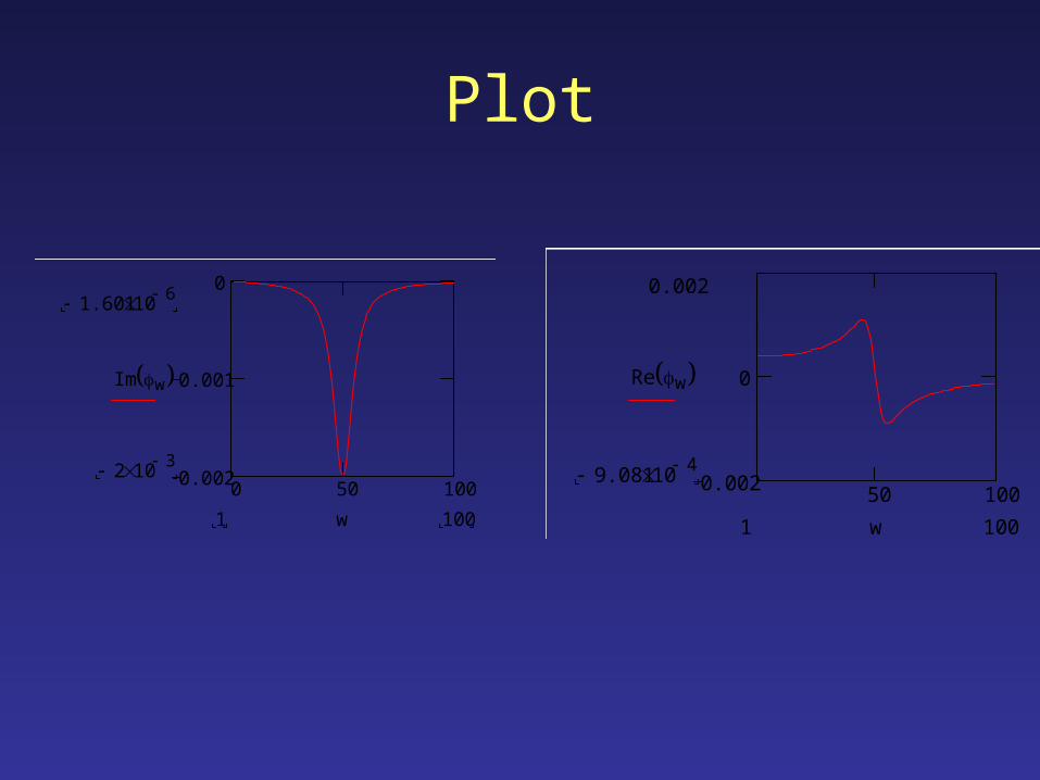
Plot

0 50 1000.002

0.001

01.601 10

6

2 103

Im w

1001 w50 100

0.002

0

0.002

9.081 104

Re w

1001 w

Profile of MRI Resonator

• Traditionally resonator thought to amplify the resonant signal

• The resonant frequency ω0 and the linewidth term Γ/2I are expressed as a ratio characterizing the sharpness of the resonance line: Q= ω0/(Γ/2I)

• This is also the resonator amplification term• ω0/Q also characterizes the width of frequencies

passed by the resonator: ω0/Q = Δω

Q.M. Time Evolution of the Magnetization

• S is the spin, an operator• H is the Hamiltonian or Energy Operator• In Heisenberg Representation:

∂S/ ∂t = 1/iћ [H,S], Recall, H= -µB∙B =- βe S ∙B. [H,Si]=HSi-SiH=-βe(SjSi-SiSj)Bj= βeiћS x B

∂S/ ∂t = βe S x B; follows also classically from the

torque on a magnetic moment ~ S x B as seen above.

Bloch Equations follow with (let M = S, M averaging over S):

∂S/ ∂t = βe S x B -1/T2(Sxî +Syĵ)-1/T1(Sz-S0)ķ

Density Matrix • Define an Operator ρ associating another operator S with

its average value:• <S> = Tr(ρS) ; ρ=Σ|ai><ai|; basically is an average over

quantum states or wavefunctions of the system• ρ : Density Matrix: Characterizes the System• ∂ρ/∂t = 1/iћ [H, ρ], 1/iћ [H0+H1, ρ],

• ρ*= exp(iH0t/ћ) ρ exp(-iH0t/ћ)=e+ ρ e-; H1*=e+H1e-

• ∂ρ*/∂t = 1/iћ [H*1(t), ρ*(t)], • ρ*~ ρ*(0) +1/iћ ∫dt’ [H*(t’)1, ρ*(0)]+ 0

(1/iћ)2 ∫dt’dt”[H*1(t’),[H*1(t”), ρ*(0)]

Here we break the Hamiltonian into two terms, the basic energy term, H0 = -µ∙B0, and a random driving term H1=µ∙Br(t), characterizing the friction of the damping

The Damping Term (Redfield)

• ∂ρ*/∂t=1/iћ [H*(t’)1, ρ*(0)]+ 0

(1/iћ)2 ∫dt’[H*1(t),[H*1(t-t’), ρ*(t’)]

• Each of the H*1 has a term in it with H= -µ∙Br and µ ~ q/m

• ∂ρ*/∂t~ (-) µ2 ρ* This is the damping term:• ρ*~exp(- µ2t with other terms)• Thus, state lifetimes, e.g. T2, are inversely

proportional to the square of the coupling constant, µ2

• The state lifetimes, e.g. T2 are proportional to the square of the mass, m2

Consequences of the Damping Term

• The coupling of the electron to the magnetic field is 103 times larger than that of a water proton so that the states relax 106 times faster

• No time for Fourier Imaging techniques• For CW we must use

1. Fixed stepped gradients 1. Vary both gradient direction & magnitude (3 angles)

2. Back projection reconstruction in 4-D

Major consequence on image technique

• µelectron=658 µproton (its not quite 1/m);• Proton has anomalous magnetic moment

due to “non point like” charge distribution (strong interaction effects)

• mproton= 1836 melectron

• Anomalous effect multiplies the magnetic moment of the proton by 2.79 so the moment ratio is 658

Relaxtion times:

• Water protons: Longitudinal relaxation times, T1 also referred to as spin lattice relaxation time ~ 1 sec

T2 transverse relaxtion time or phase coherence time ~ 100s of milliseconds• Electrons

T1e 100s of ns to µs

T2e 10s of ns to µs

Magnetization: Magnetic Resonance Experiment

• Above touches on the important concept ofmagnetization M as opposed to

spin S

• From the above, M=Tr(ρS), • Thus magnetization M is an average of the spin

operator over the states of the spin system• These can be

– coherently prepared or,– as is most often the case, incoherent states – Or mixed coherent and incoherent

Magnetization

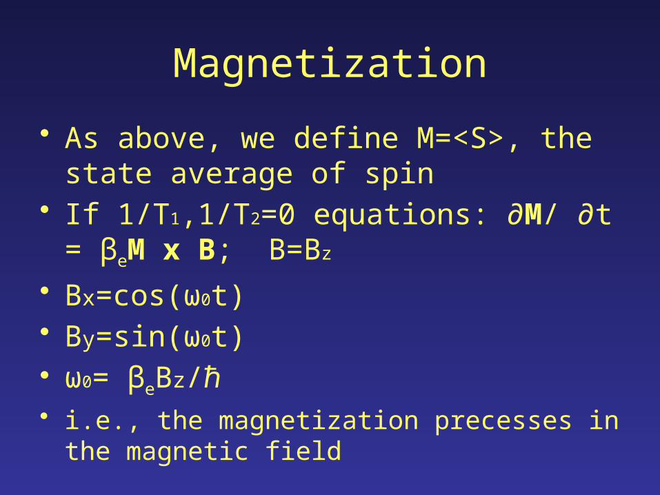
• As above, we define M=<S>, the state average of spin

• If 1/T1,1/T2=0 equations: ∂M/ ∂t = βeM x B; B=Bz

• Bx=cos(ω0t)• By=sin(ω0t)• ω0= βeBz/ℏ

• i.e., the magnetization precesses in the magnetic field

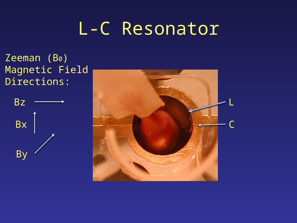
L-C Resonator

C

L

Zeeman (B0)Magnetic Field Directions:

Bz

Bx

By

Resonator Functions

1. Generate Radiofrequency/Microwave fields to stimulate resonant absorption and dispersion at resonance condition: hn=mB0

2. Sense the precessing induction from the spin sample

1. Spin sample magnetization M couples through resonator inductance

2. Creates an oscillating voltage at the resonator output

Two modes

• Continuous wave detection• Pulse

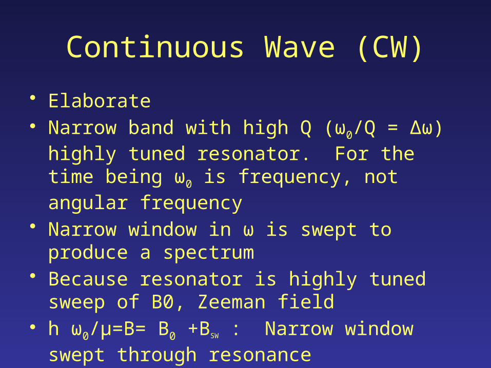
Continuous Wave (CW)

• Elaborate• Narrow band with high Q (ω0/Q = Δω) highly tuned

resonator. For the time being ω0 is frequency, not angular frequency

• Narrow window in ω is swept to produce a spectrum• Because resonator is highly tuned sweep of B0,

Zeeman field• h ω0/μ=B= B0 +BSW : Narrow window swept through

resonance

Bridge

• Generally the resonator is part of a “bridge” analogous to the Wheatstone bridge to measure a resistance by balancing voltage drops across resistance and zeroing the current

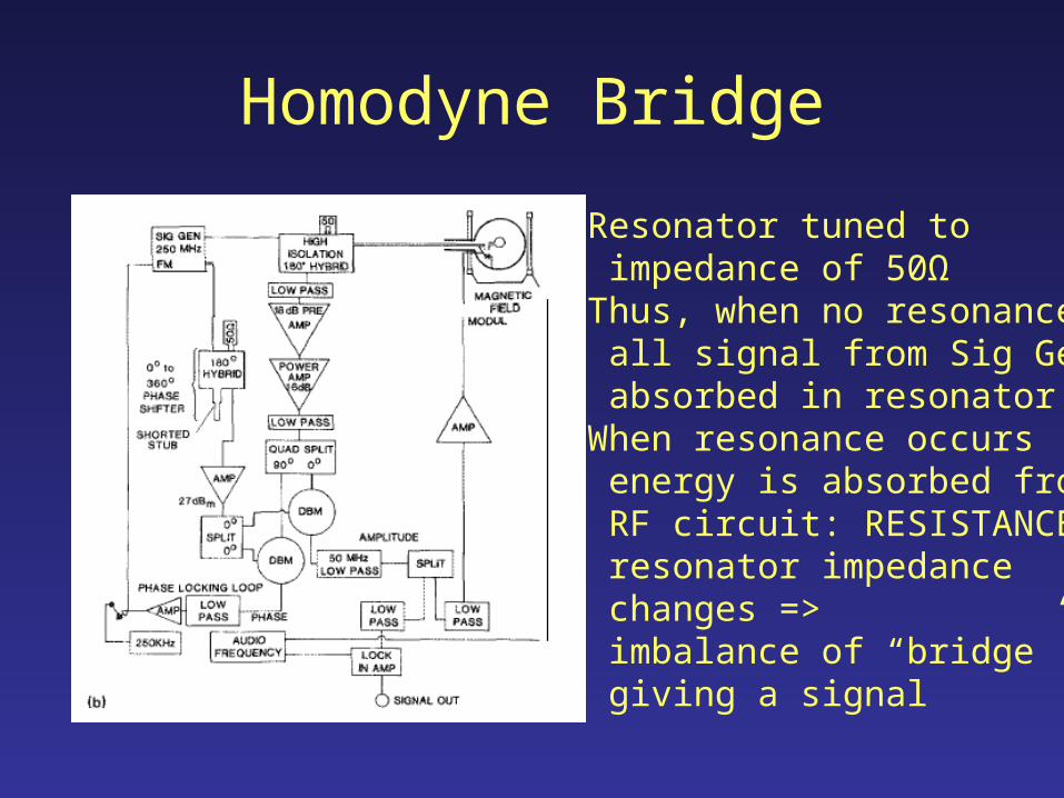
Homodyne Bridge

Resonator tuned to impedance of 50ΩThus, when no resonance all signal from Sig Gen absorbed in resonatorWhen resonance occurs energy is absorbed from RF circuit: RESISTANCE resonator impedance changes => imbalance of “bridge” giving a signal

For this “Bridge” balance with system impedance (resistance): 50 Ω• Resonance involves absorption of energy from the RF

circuit, appearing as a proportional resistance • Bridge loses balance: resonator impedance no longer

50 Ω.• Signal: 250 MHz voltage• Mixers combine reference from SIG GEN• Multiply Acoswt*coswt= A[cos( + )w w t+cos( -w

)w t]=A + high frequency which we filter• Demodulating the Carrier Frequency.

More

• Field modulation• Very low frequency “baseline” drift: 1/f noise• Solution: Zeeman field modulation• Add to B0 a Bmod=coswmodt term where wmod is

~audio frequency.• Detect with a Lock-in amplifier whose output is the

input amplitude at a multiple (harmonic) of wmod • First harmonic ~ first derivative like spectrum

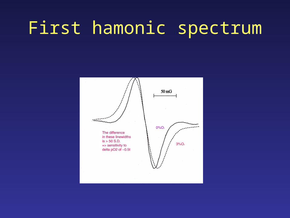
First hamonic spectrum

Pulse

• Offensive lineman’s approach to magnetic resonance• Depositing a broad-band pulse into the spin system

and then detect its precession and its decay times• CW: driving a harmonic oscillator with frequency w

and measuring amplitude response• Pulse: striking mass on spring and measuring

oscillation response including many modes each with– A frequency– An amplitude– Fourier transform give spectral frequency response

Broadband Pulse

• Real Uncertainty principle in signal theory:• ΔνΔT=1• Exercise: For a signal with temporal

distribution F(t)=exp(-t^2) what is the product of the FWHH of the temporal distribution and that of its Fourier transform?

• What is that of F(t)=exp(-(at)^2)?

MRI broadband

• ΔT=1μs• Δν=1 MHz• Water proton gyromagnetic ratio: 42

MH/T• => 1μs pulse give 0.024 T excitation

(.24 KGauss)

EPR Broadband

• 1 ns pulse => 1 GHz excitation• Electron gyromagnetic ratio: 28 GHz/T• 1 ns pulse gives 0.035 T wide excitation• NMR lines typically much narrower than EPR• EPR is a hard way to live

Pulse bridge

• Simpler particularly for MRI• Requires same carrier demodulation• Requires lower Q for broad pass band• Excites all spins in the passband window so, in

principle, more efficient acqusition

Magnetic field gradients encode position or location

• Postulated by Lauterbur in landmark 1973 Nature paper

• Overcomes diffraction limit on 40 MHz RF– λ = 7.5 m

• Gradient: Gi= dB/dxi where x1=x; x2=y; x3=z• B is likewise a vector but generally take to be

Bz.

Standard MRI z slice selection

• z dimension distinguished by pulsing a large gradient during the acqusition

• GzΔz = ∂Bz/∂zΔz = ΔB = hΔν/βe

• Δν = GzΔz/hβe

• If Δν > ω0/Q the frequency pass band of the resonator, then the sensitive slice thickness is defined by Δz= hβeω0/QGz

X and Y location encoding

• For standard water proton MRI, within the z selected plane

• Apply Gradient Gx-Gy plane• Frequency and phase encoding

Phase encoding

• Generally one of the Gx or Gy direction generating gradients selected. Say Gy

• The gradient is pulsed for a fixed time Δt before signal from the precessing magnetization is measured.

• Magnetization develops a phase proportional to the distance along the y coordinate Δφ=2πyGy/βp where βp is the proton gyromagnetic ratio.

Frequency Encoding

• The orthogonal direction say x has the gradient imposed in that direction during the acquisition of the magnetization precession signal

• This shifts the frequency of the precession proportional to the x coordinate magnitude Δω=xGx

Signal Amplitude vs location

• The complex Fourier transform of the voltage induced in the resonator by the precession of the magnetization gives the signal amplitude as a function of frequency and phase

• The signal amplitude as a function of these parameters is the amplitude of the magnetization as a function of location in the sample

EPR: No time for Phase Encoding

• Generally use fixed stepped gradients• Both for CW and Pulse• Tomographic or FBP based reconstruction

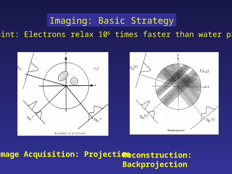
Imaging: Basic Strategy

Constraint: Electrons relax 106 times faster than water protons

Image Acquisition: Projection Reconstruction: Backprojection

Key for EPR Images

• Spectroscopic imaging• Obtain a spectrum from each voxel• EPRI usually uses an injected reporter

molecule• Spectral information from the reporter

molecule from each voxel quantitatively reports condition of the fluids of the distribution volume of the reporter

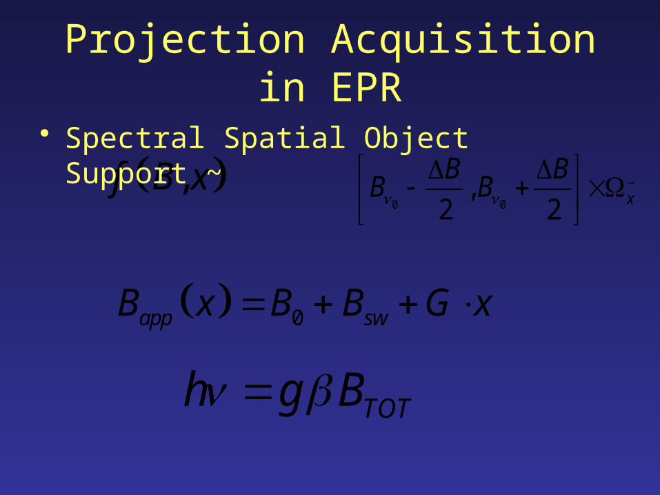
Projection Acquisition in EPR

,f B x

0 0,

2 2 x

B BB B

0app swB x B B G x

• Spectral Spatial Object Support ~

TOTh g B

=α

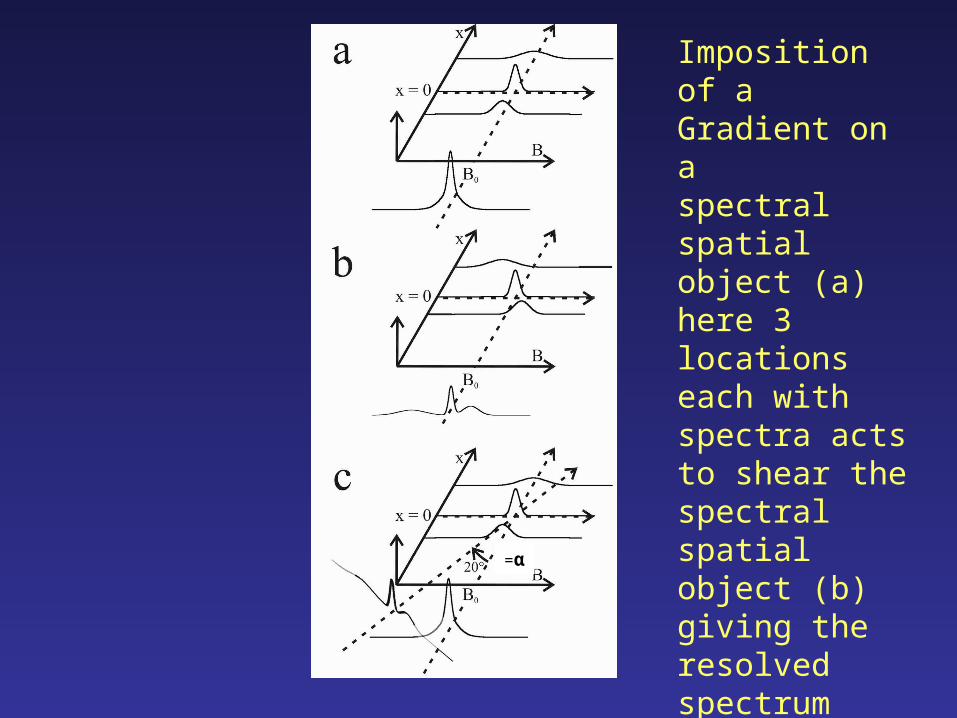
Imposition of a Gradient on aspectral spatialobject (a) here 3 locations each with spectra acts to shear the spectral spatial object (b) giving the resolved spectrum shown. This is equivalent to observing (a) at an angle a (c). This is a Spectral-Spatial Projection.

Projection Description

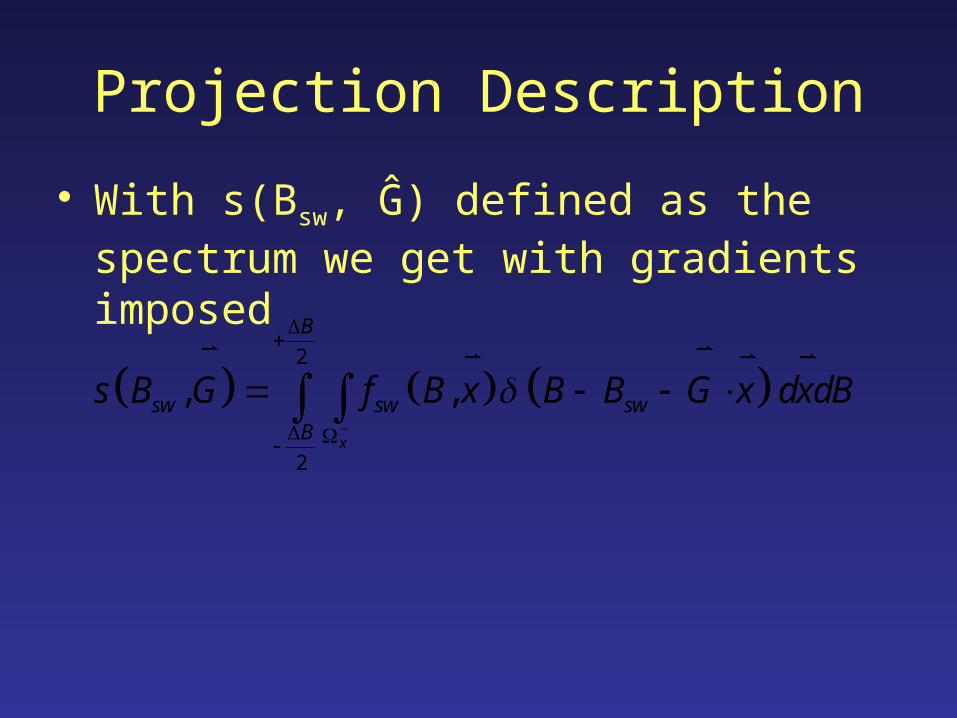
• With s(Bsw, Ĝ) defined as the spectrum we get with gradients imposed

2

2

, ,x

B

sw sw swB

s B G f B x B B G x dxdB

More Projection

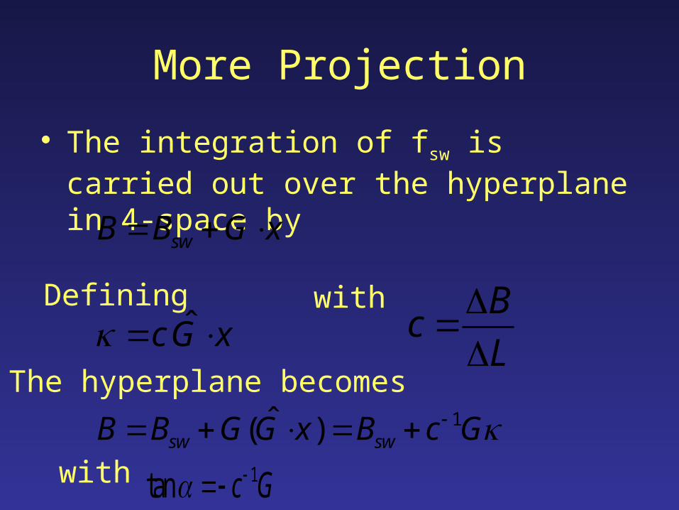
• The integration of fsw is carried out over the hyperplane in 4-space by

swB B G x

DefiningˆcG x

Bc

L

with

The hyperplane becomes1ˆ( )sw swB B G G x B c G

with 1tan c G

And a Little More

2

2

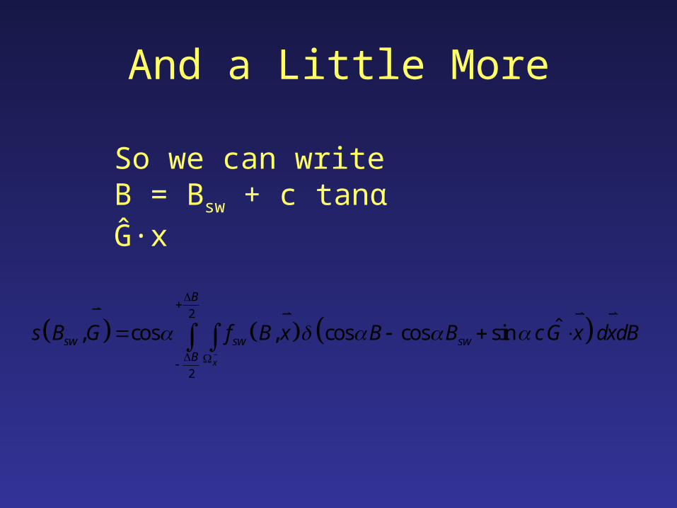
ˆ, cos , cos cos sinx

B

sw sw swB

s B G f B x B B cG x dxdB

So we can write B = Bsw + c tanα Ĝ∙x

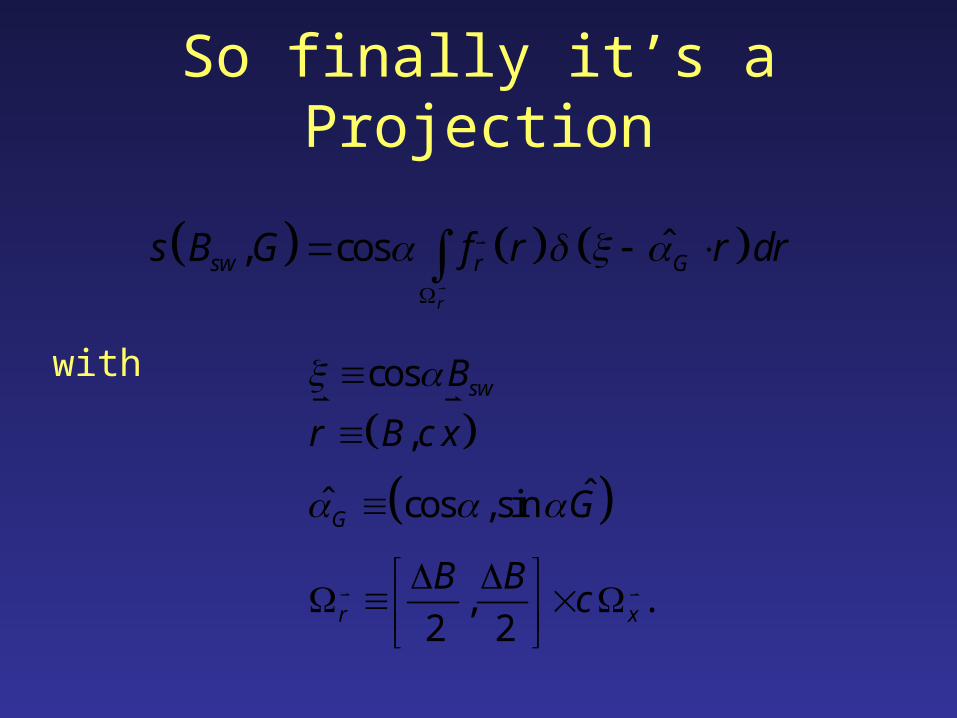
So finally it’s a Projection

ˆ, cosr

sw r Gs B G f r r dr

with

cos

,

ˆˆ cos ,sin

, .2 2

sw

G

r x

B

r B c x

G

B Bc

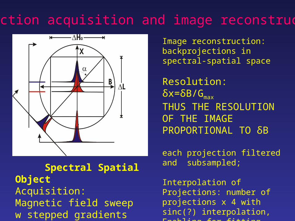
Projection acquisition and image reconstruction

Image reconstruction: backprojections in spectral-spatial space

Resolution: δx=δB/Gmax THUS THE RESOLUTION OF THE IMAGE PROPORTIONAL TO δB

each projection filtered and subsampled;

Interpolation of Projections: number of projections x 4 with sinc(?) interpolation,Enabling for fitting

Spectral Spatial ObjectAcquisition: Magnetic field sweep w stepped gradients (G)Projections: Angle a: tan( )a =G*DL/DH

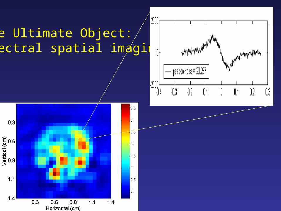
The Ultimate Object:Spectral spatial imaging

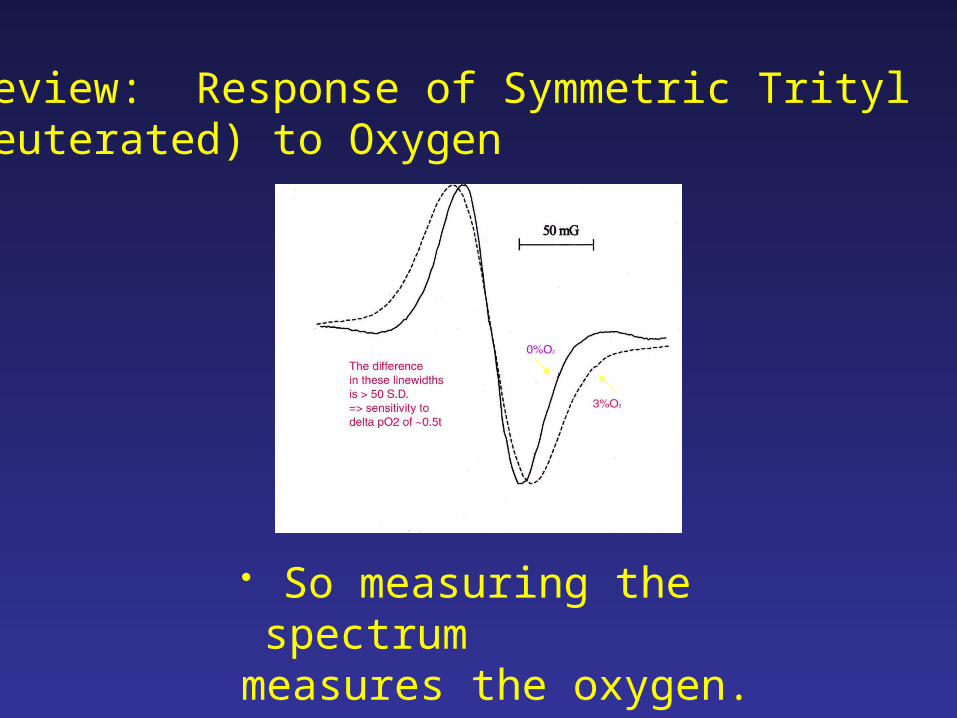
Preview: Response of Symmetric Trityl (deuterated) to Oxygen

• So measuring the spectrummeasures the oxygen. Imaging the spectrum: Oxygen Image