Embed Size (px)
Citation preview
University of UtahMathematical Biology
theImagine Possibilities
Introduction to PhysiologyII: Control of Cell Volume and Membrane
Potential
J. P. Keener
Mathematics Department
University of Utah
Math Physiology – p.1/23
University of UtahMathematical Biology
theImagine Possibilities
Basic Problem
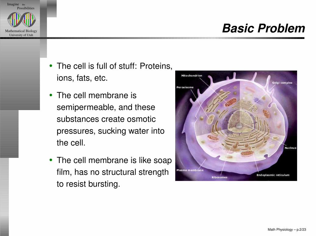
• The cell is full of stuff: Proteins,ions, fats, etc.
• The cell membrane issemipermeable, and thesesubstances create osmoticpressures, sucking water intothe cell.
• The cell membrane is like soapfilm, has no structural strengthto resist bursting.
Math Physiology – p.2/23
University of UtahMathematical Biology
theImagine Possibilities
Basic Solution
• Carefully regulate the intracellular ionic concentrations sothat there are no net osmotic pressures.
• As a result, the major ions (Na+, K+, Cl− and Ca++) havedifferent intracellular and extracellular concentrations.
• Consequently, there is an electrical potential differenceacross the cell membrane, the membrane potential.
Math Physiology – p.3/23
University of UtahMathematical Biology
theImagine Possibilities
Membrane Transporters
+
+ ++KNa
+
ATP
Na
� � � � � � � � � � � � � � � � � � � � � � � � � � � � � � � � � � � � � � � � � � � � � � � � � � � � �
� � � � � � � � � � � � � � � � � � � � � � � � � � � � � � � � � � � � � � � � � � � � � � � � � � � � �
� � � � � � � � � � � � � � � � � � � � � � � � � � � � � � � � � � � � � � � � � � � � � � � � � � � � �
� � � � � � � � � � � � � � � � � � � � � � � � � � � � � � � � � � � � � � � � � � � � � � � � � � � � �
� � � � � � � � � � � � � � � � � � � � � � � � � � � � � � � � � � � � � � � � � � � � � � � � � � � � �
O CO2 2
GlucoseH O2
+CaK
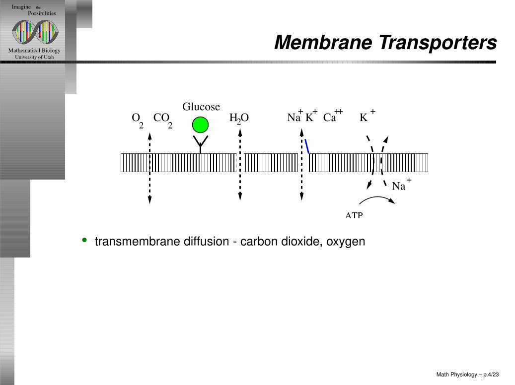
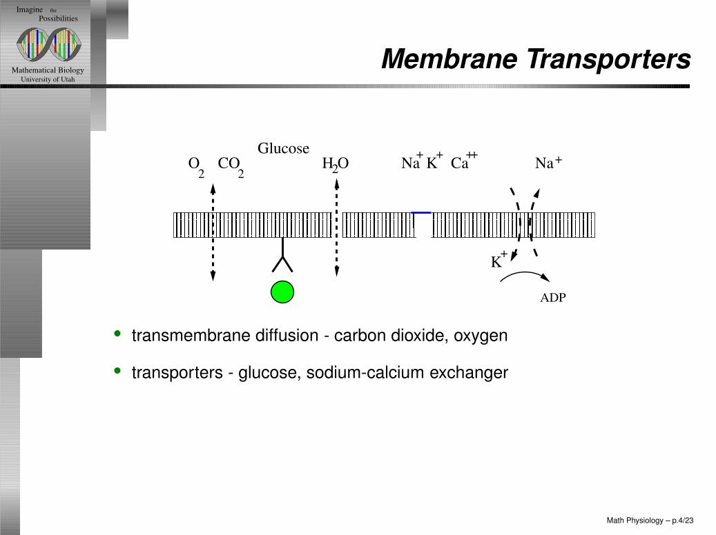
• transmembrane diffusion - carbon dioxide, oxygen
• transporters - glucose, sodium-calcium exchanger
• pores - water
• ion-selective, gated channels - sodium, potassium, calcium
• ATPase exchangers - sodium-potassium ATPase, SERCA
Math Physiology – p.4/23
University of UtahMathematical Biology
theImagine Possibilities
Membrane Transporters
+
++Na Na+
ADP
K
� � � � � � � � � � � � � � � � � � � � � � � � � � � � � � � � � � � � � � � � � � � � � � � � � � � � � �
� � � � � � � � � � � � � � � � � � � � � � � � � � � � � � � � � � � � � � � � � � � � � � � � � � � � � �
� � � � � � � � � � � � � � � � � � � � � � � � � � � � � � � � � � � � � � � � � � � � � � � � � � � � �
� � � � � � � � � � � � � � � � � � � � � � � � � � � � � � � � � � � � � � � � � � � � � � � � � � � � �
O CO2 2
GlucoseH O2
+CaK
+
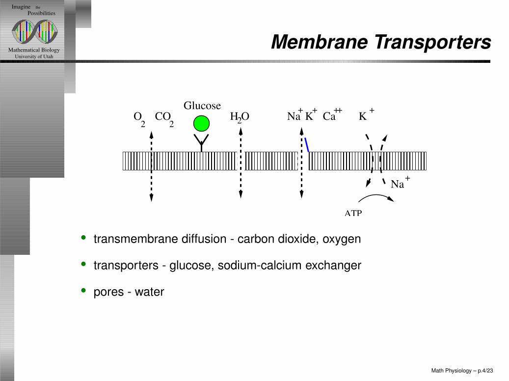
• transmembrane diffusion - carbon dioxide, oxygen
• transporters - glucose, sodium-calcium exchanger
• pores - water
• ion-selective, gated channels - sodium, potassium, calcium
• ATPase exchangers - sodium-potassium ATPase, SERCA
Math Physiology – p.4/23
University of UtahMathematical Biology
theImagine Possibilities
Membrane Transporters
+
+ ++KNa
+
ATP
Na
� � � � � � � � � � � � � � � � � � � � � � � � � � � � � � � � � � � � � � � � � � � � � � � � � � � � �
� � � � � � � � � � � � � � � � � � � � � � � � � � � � � � � � � � � � � � � � � � � � � � � � � � � � �
� � � � � � � � � � � � � � � � � � � � � � � � � � � � � � � � � � � � � � � � � � � � � � � � � � � � �
� � � � � � � � � � � � � � � � � � � � � � � � � � � � � � � � � � � � � � � � � � � � � � � � � � � � �
� � � � � � � � � � � � � � � � � � � � � � � � � � � � � � � � � � � � � � � � � � � � � � � � � � � � �
O CO2 2
GlucoseH O2
+CaK
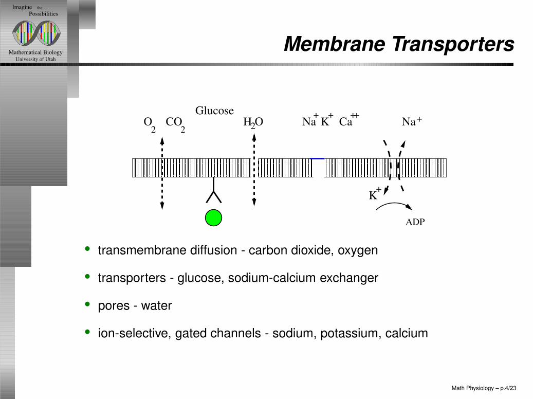
• transmembrane diffusion - carbon dioxide, oxygen
• transporters - glucose, sodium-calcium exchanger
• pores - water
• ion-selective, gated channels - sodium, potassium, calcium
• ATPase exchangers - sodium-potassium ATPase, SERCA
Math Physiology – p.4/23
University of UtahMathematical Biology
theImagine Possibilities
Membrane Transporters
+
++Na Na+
ADP
K
� � � � � � � � � � � � � � � � � � � � � � � � � � � � � � � � � � � � � � � � � � � � � � � � � � � � � �
� � � � � � � � � � � � � � � � � � � � � � � � � � � � � � � � � � � � � � � � � � � � � � � � � � � � � �
� � � � � � � � � � � � � � � � � � � � � � � � � � � � � � � � � � � � � � � � � � � � � � � � � � � � �
� � � � � � � � � � � � � � � � � � � � � � � � � � � � � � � � � � � � � � � � � � � � � � � � � � � � �
O CO2 2
GlucoseH O2
+CaK
+
• transmembrane diffusion - carbon dioxide, oxygen
• transporters - glucose, sodium-calcium exchanger
• pores - water
• ion-selective, gated channels - sodium, potassium, calcium
• ATPase exchangers - sodium-potassium ATPase, SERCA
Math Physiology – p.4/23

University of UtahMathematical Biology
theImagine Possibilities
Membrane Transporters
+
+ ++KNa
+
ATP
Na
� � � � � � � � � � � � � � � � � � � � � � � � � � � � � � � � � � � � � � � � � � � � � � � � � � � � �
� � � � � � � � � � � � � � � � � � � � � � � � � � � � � � � � � � � � � � � � � � � � � � � � � � � � �
� � � � � � � � � � � � � � � � � � � � � � � � � � � � � � � � � � � � � � � � � � � � � � � � � � � � �
O CO2 2
GlucoseH O2
+CaK
• transmembrane diffusion - carbon dioxide, oxygen
• transporters - glucose, sodium-calcium exchanger
• pores - water
• ion-selective, gated channels - sodium, potassium, calcium
• ATPase exchangers - sodium-potassium ATPase, SERCA
Math Physiology – p.4/23
University of UtahMathematical Biology
theImagine Possibilities
How Things Move
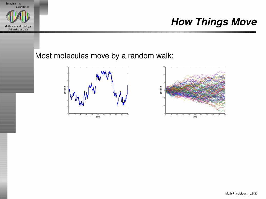
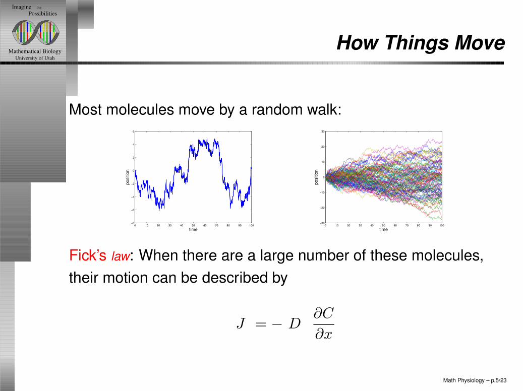
Most molecules move by a random walk:
0 10 20 30 40 50 60 70 80 90 100−8
−6
−4
−2
0
2
4
6
time
posi
tion
0 10 20 30 40 50 60 70 80 90 100−30
−20
−10
0
10
20
30
time
posi
tion
Fick’s law: When there are a large number of these molecules,their motion can be described by
Math Physiology – p.5/23
University of UtahMathematical Biology
theImagine Possibilities
How Things Move
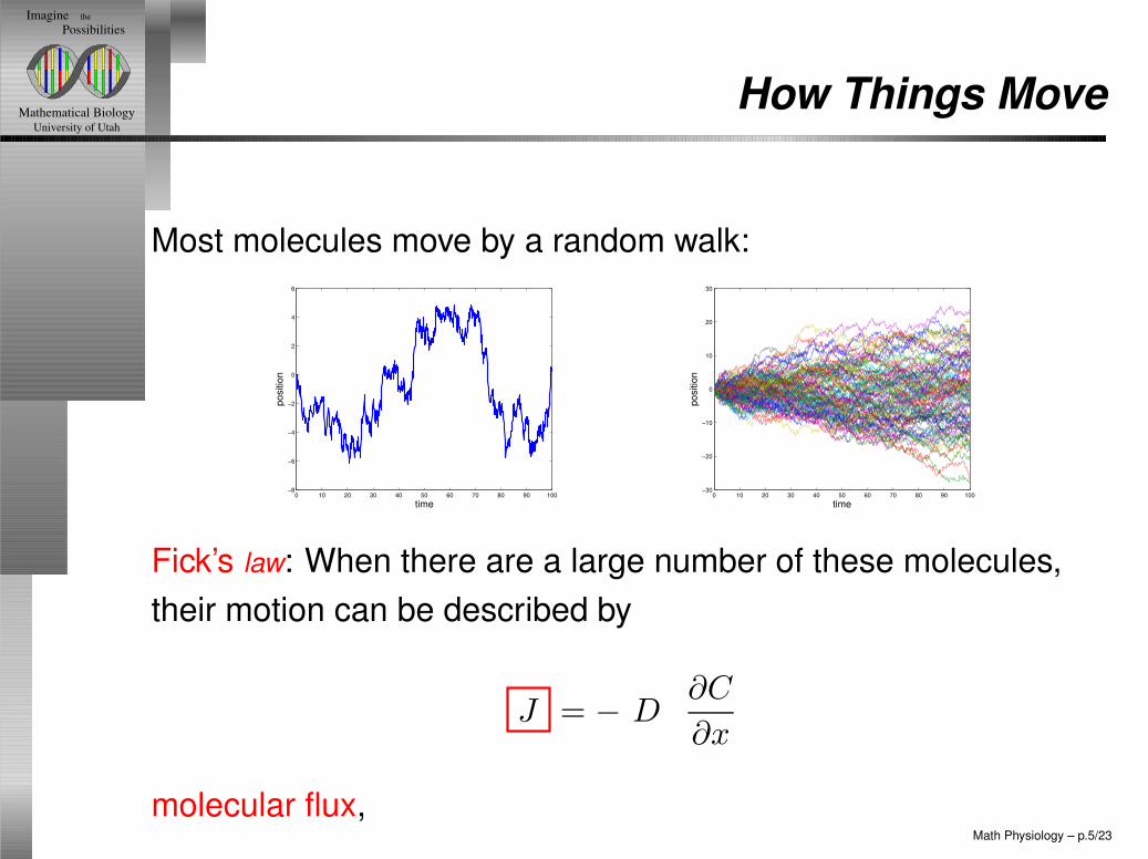
Most molecules move by a random walk:
0 10 20 30 40 50 60 70 80 90 100−8
−6
−4
−2
0
2
4
6
time
posi
tion
0 10 20 30 40 50 60 70 80 90 100−30
−20
−10
0
10
20
30
time
posi
tion
Fick’s law: When there are a large number of these molecules,their motion can be described by
J = − D∂C
∂x
Math Physiology – p.5/23
University of UtahMathematical Biology
theImagine Possibilities
How Things Move
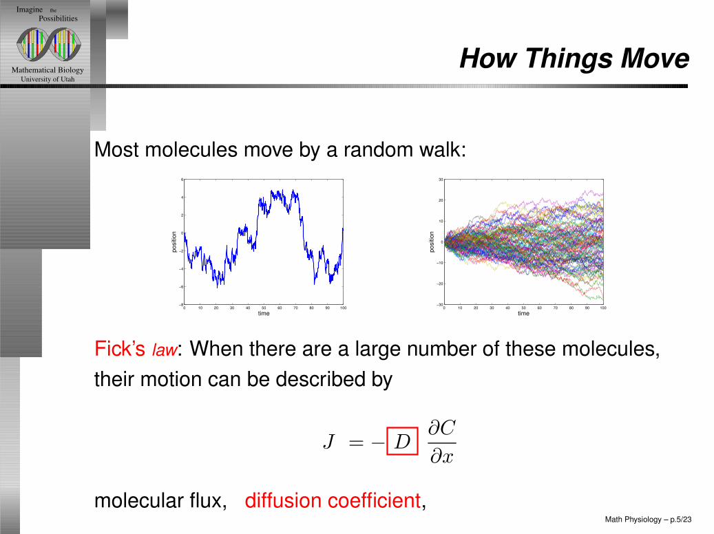
Most molecules move by a random walk:
0 10 20 30 40 50 60 70 80 90 100−8
−6
−4
−2
0
2
4
6
time
posi
tion
0 10 20 30 40 50 60 70 80 90 100−30
−20
−10
0
10
20
30
time
posi
tion
Fick’s law: When there are a large number of these molecules,their motion can be described by
J = − D∂C
∂x
molecular flux,Math Physiology – p.5/23
University of UtahMathematical Biology
theImagine Possibilities
How Things Move
Most molecules move by a random walk:
0 10 20 30 40 50 60 70 80 90 100−8
−6
−4
−2
0
2
4
6
time
posi
tion
0 10 20 30 40 50 60 70 80 90 100−30
−20
−10
0
10
20
30
time
posi
tion
Fick’s law: When there are a large number of these molecules,their motion can be described by
J = − D∂C
∂x
molecular flux, diffusion coefficient,Math Physiology – p.5/23
University of UtahMathematical Biology
theImagine Possibilities
How Things Move
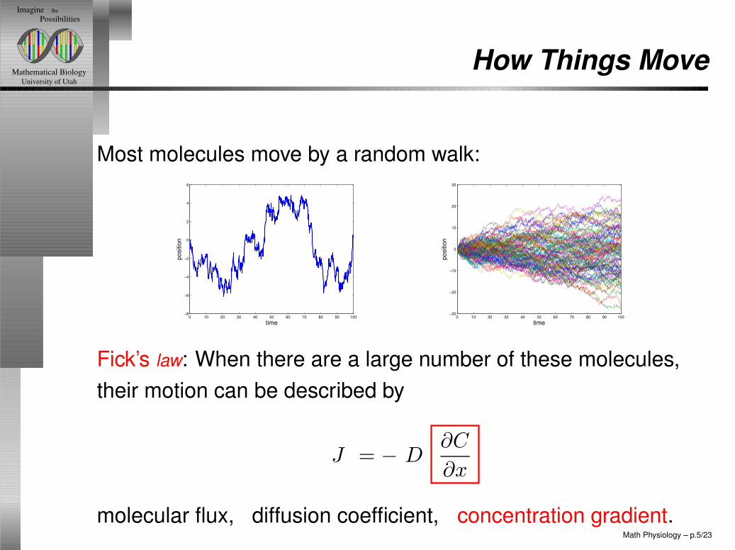
Most molecules move by a random walk:
0 10 20 30 40 50 60 70 80 90 100−8
−6
−4
−2
0
2
4
6
time
posi
tion
0 10 20 30 40 50 60 70 80 90 100−30
−20
−10
0
10
20
30
time
posi
tion
Fick’s law: When there are a large number of these molecules,their motion can be described by
J = − D∂C
∂x
molecular flux, diffusion coefficient, concentration gradient.Math Physiology – p.5/23
University of UtahMathematical Biology
theImagine Possibilities
Conservation Law
Conservation:∂C
∂t+
∂J
∂x= 0
leading to the Diffusion Equation
∂C
∂t=
∂
∂x(D
∂C
∂x).
Math Physiology – p.6/23
University of UtahMathematical Biology
theImagine Possibilities
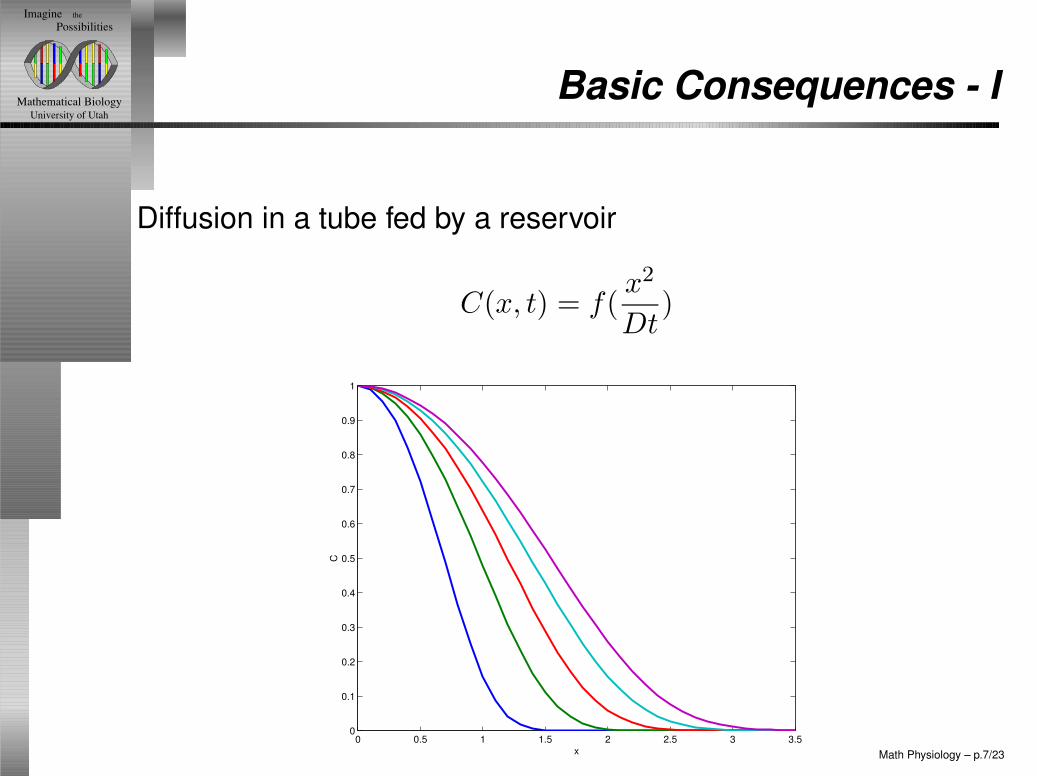
Basic Consequences - I
Diffusion in a tube fed by a reservoir
C(x, t) = f(x2
Dt)
0 0.5 1 1.5 2 2.5 3 3.50
0.1
0.2
0.3
0.4
0.5
0.6
0.7
0.8
0.9
1
x
C
Math Physiology – p.7/23
University of UtahMathematical Biology
theImagine Possibilities
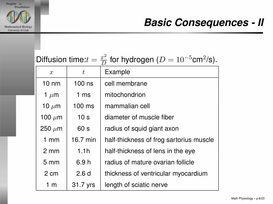
Basic Consequences - II
Diffusion time:t = x2
Dfor hydrogen (D = 10−5cm2/s).
x t Example
10 nm 100 ns cell membrane
1 µm 1 ms mitochondrion
10 µm 100 ms mammalian cell
100 µm 10 s diameter of muscle fiber
250 µm 60 s radius of squid giant axon
1 mm 16.7 min half-thickness of frog sartorius muscle
2 mm 1.1h half-thickness of lens in the eye
5 mm 6.9 h radius of mature ovarian follicle
2 cm 2.6 d thickness of ventricular myocardium
1 m 31.7 yrs length of sciatic nerve
Math Physiology – p.8/23
University of UtahMathematical Biology
theImagine Possibilities
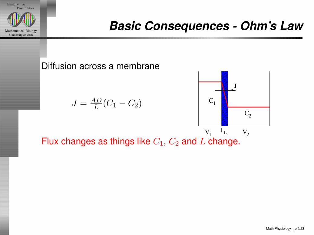
Basic Consequences - Ohm’s Law
Diffusion across a membrane
J = ADL
(C1 − C2)
��
����
����
����
���
V
C2
1 V2L
C1
J
Flux changes as things like C1, C2 and L change.
Math Physiology – p.9/23

University of UtahMathematical Biology
theImagine Possibilities
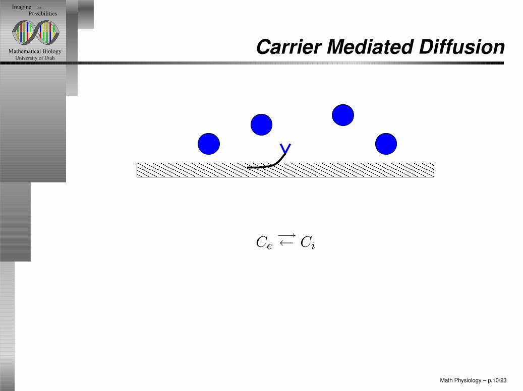
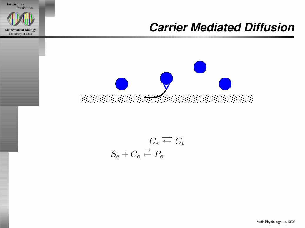
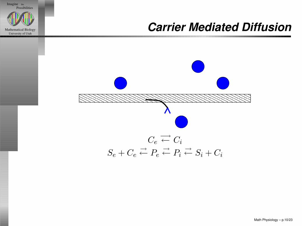
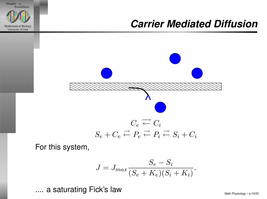
Carrier Mediated Diffusion
� � � � � � � � � � � � � � � � � � � � �� � � � � � � � � � � � � � � � � � � � �
Ce−→
← Ci
Se + Ce→
← Pe→
← Pi→
← Si + Ci
For this system,
J = JmaxSe − Si
(Se + Ke)(Si + Ki).
.... a saturating Fick’s law
Math Physiology – p.10/23

University of UtahMathematical Biology
theImagine Possibilities
Carrier Mediated Diffusion
� � � � � � � � � � � � � � � � � � � � �� � � � � � � � � � � � � � � � � � � � �� � � � � � � � � � � � � � � � � � � � �� � � � � � � � � � � � � � � � � � � � �
Ce−→
← Ci
Se + Ce→
← Pe→
← Pi→
← Si + Ci
For this system,
J = JmaxSe − Si
(Se + Ke)(Si + Ki).
.... a saturating Fick’s law
Math Physiology – p.10/23
University of UtahMathematical Biology
theImagine Possibilities
Carrier Mediated Diffusion
� � � � � � � � � � � � � � � � � � � � �� � � � � � � � � � � � � � � � � � � � �� � � � � � � � � � � � � � � � � � � � �� � � � � � � � � � � � � � � � � � � � �
Ce−→
← Ci
Se + Ce→
← Pe
→
← Pi→
← Si + Ci
For this system,
J = JmaxSe − Si
(Se + Ke)(Si + Ki).
.... a saturating Fick’s law
Math Physiology – p.10/23

University of UtahMathematical Biology
theImagine Possibilities
Carrier Mediated Diffusion
� � � � � � � � � � � � � � � � � � � � �� � � � � � � � � � � � � � � � � � � � �� � � � � � � � � � � � � � � � � � � � �� � � � � � � � � � � � � � � � � � � � �
Ce−→
← Ci
Se + Ce→
← Pe→
← Pi
→
← Si + Ci
For this system,
J = JmaxSe − Si
(Se + Ke)(Si + Ki).
.... a saturating Fick’s law
Math Physiology – p.10/23
University of UtahMathematical Biology
theImagine Possibilities
Carrier Mediated Diffusion
� � � � � � � � � � � � � � � � � � � � �� � � � � � � � � � � � � � � � � � � � �� � � � � � � � � � � � � � � � � � � � �� � � � � � � � � � � � � � � � � � � � �
Ce−→
← Ci
Se + Ce→
← Pe→
← Pi→
← Si + Ci
For this system,
J = JmaxSe − Si
(Se + Ke)(Si + Ki).
.... a saturating Fick’s law
Math Physiology – p.10/23
University of UtahMathematical Biology
theImagine Possibilities
Carrier Mediated Diffusion
� � � � � � � � � � � � � � � � � � � � �� � � � � � � � � � � � � � � � � � � � �� � � � � � � � � � � � � � � � � � � � �� � � � � � � � � � � � � � � � � � � � �
Ce−→
← Ci
Se + Ce→
← Pe→
← Pi→
← Si + Ci
For this system,
J = JmaxSe − Si
(Se + Ke)(Si + Ki).
.... a saturating Fick’s lawMath Physiology – p.10/23
University of UtahMathematical Biology
theImagine Possibilities
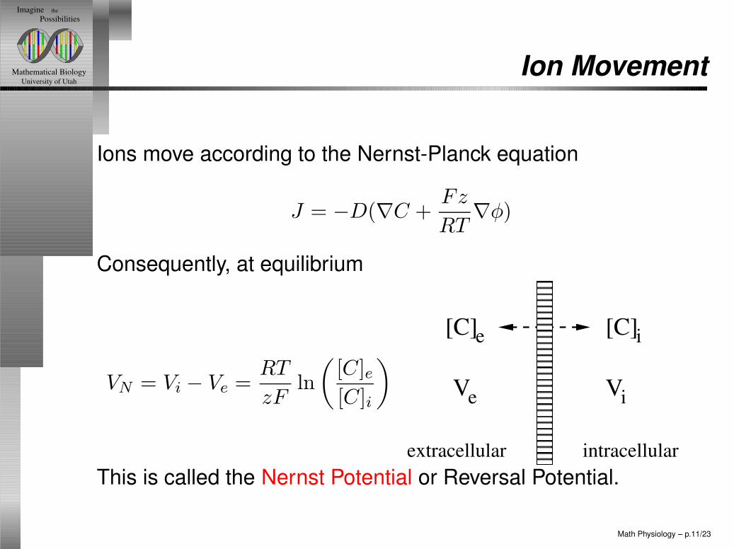
Ion Movement
Ions move according to the Nernst-Planck equation
J = −D(∇C +Fz
RT∇φ)
Consequently, at equilibrium
VN = Vi − Ve =RT
zFln
(
[C]e[C]i
)
i
Ve Vi
extracellular intracellular
[C] [C]e
This is called the Nernst Potential or Reversal Potential.
Math Physiology – p.11/23
University of UtahMathematical Biology
theImagine Possibilities
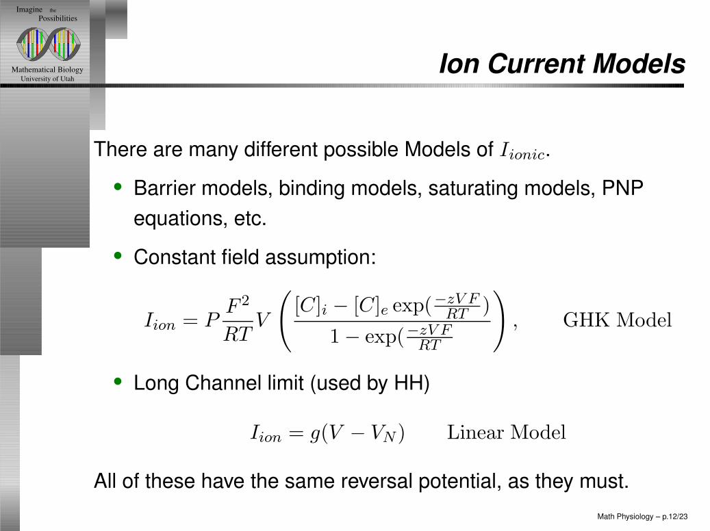
Ion Current Models
There are many different possible Models of Iionic.
• Barrier models, binding models, saturating models, PNPequations, etc.
• Constant field assumption:
Iion = PF 2
RTV
(
[C]i − [C]e exp(−zV FRT
)
1− exp(−zV FRT
)
, GHK Model
• Long Channel limit (used by HH)
Iion = g(V − VN ) Linear Model
All of these have the same reversal potential, as they must.Math Physiology – p.12/23
University of UtahMathematical Biology
theImagine Possibilities
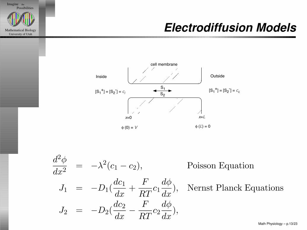
Electrodiffusion Models
x=0 x=L
[S1+] = [S2
-] = ci[S1
+] = [S2-] = ce
S1
S2
Inside Outside
φ (0) = V φ (L) = 0
cell membrane
d2φ
dx2= −λ2(c1 − c2), Poisson Equation
J1 = −D1(dc1
dx+
F
RTc1
dφ
dx), Nernst Planck Equations
J2 = −D2(dc2
dx−
F
RTc2
dφ
dx),
Math Physiology – p.13/23
University of UtahMathematical Biology
theImagine Possibilities
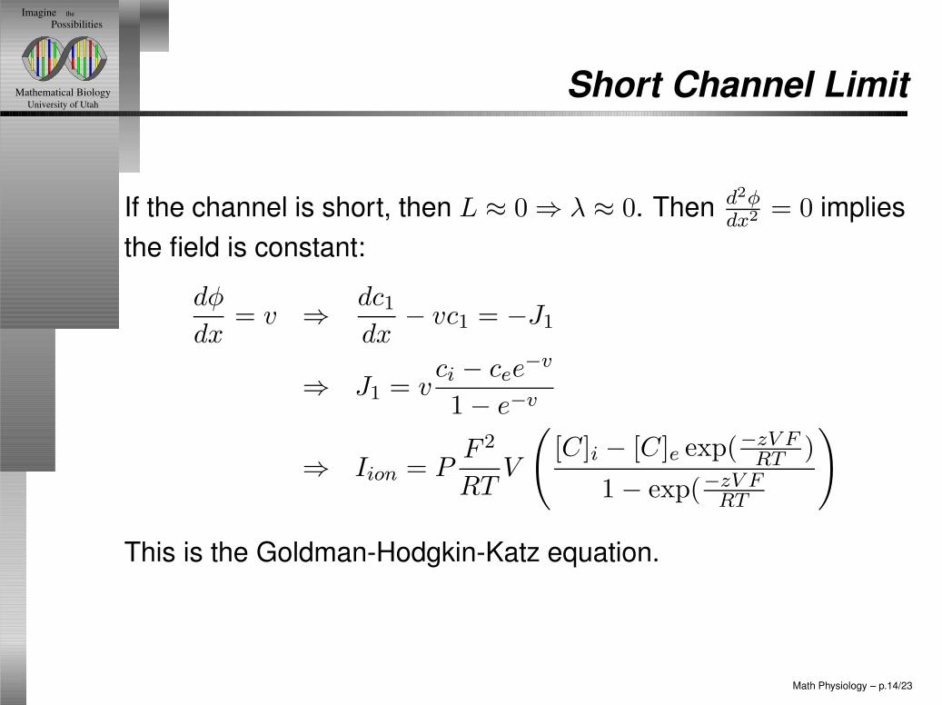
Short Channel Limit
If the channel is short, then L ≈ 0⇒ λ ≈ 0. Then d2φdx2 = 0 implies
the field is constant:
dφ
dx= v ⇒
dc1
dx− vc1 = −J1
⇒ J1 = vci − cee
−v
1− e−v
⇒ Iion = PF 2
RTV
(
[C]i − [C]e exp(−zV FRT
)
1− exp(−zV FRT
)
This is the Goldman-Hodgkin-Katz equation.
Math Physiology – p.14/23
University of UtahMathematical Biology
theImagine Possibilities
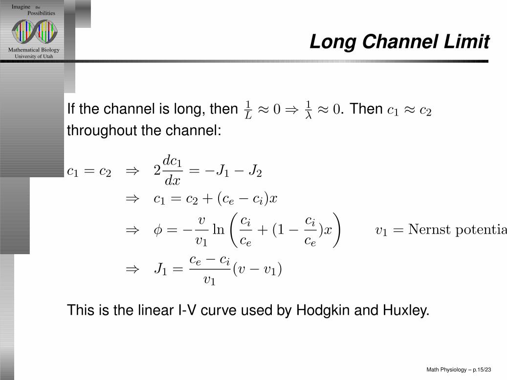
Long Channel Limit
If the channel is long, then 1
L≈ 0⇒ 1
λ≈ 0. Then c1 ≈ c2
throughout the channel:
c1 = c2 ⇒ 2dc1
dx= −J1 − J2
⇒ c1 = c2 + (ce − ci)x
⇒ φ = −v
v1
ln
(
ci
ce+ (1−
ci
ce)x
)
v1 = Nernst potential
⇒ J1 =ce − ci
v1
(v − v1)
This is the linear I-V curve used by Hodgkin and Huxley.
Math Physiology – p.15/23
University of UtahMathematical Biology
theImagine Possibilities
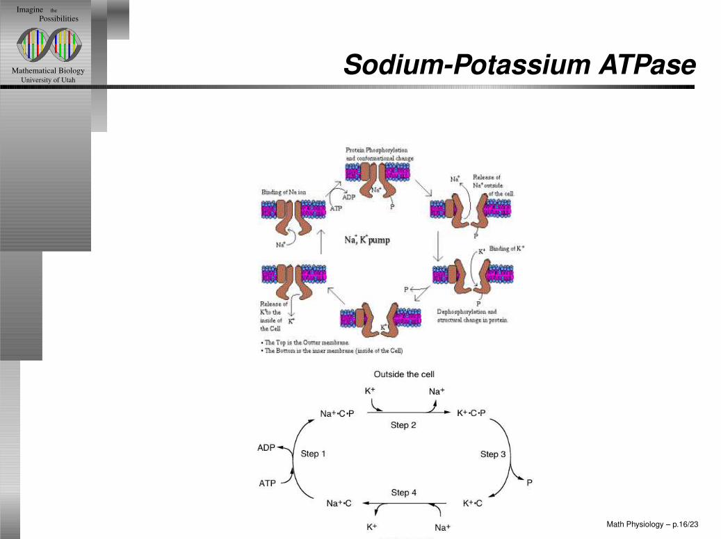
Sodium-Potassium ATPase
Math Physiology – p.16/23
University of UtahMathematical Biology
theImagine Possibilities
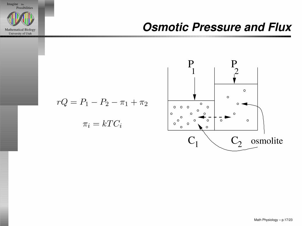
Osmotic Pressure and Flux
rQ = P1 − P2 − π1 + π2
πi = kTCi
osmolite
P P1 2
C C1 2
Math Physiology – p.17/23
University of UtahMathematical Biology
theImagine Possibilities
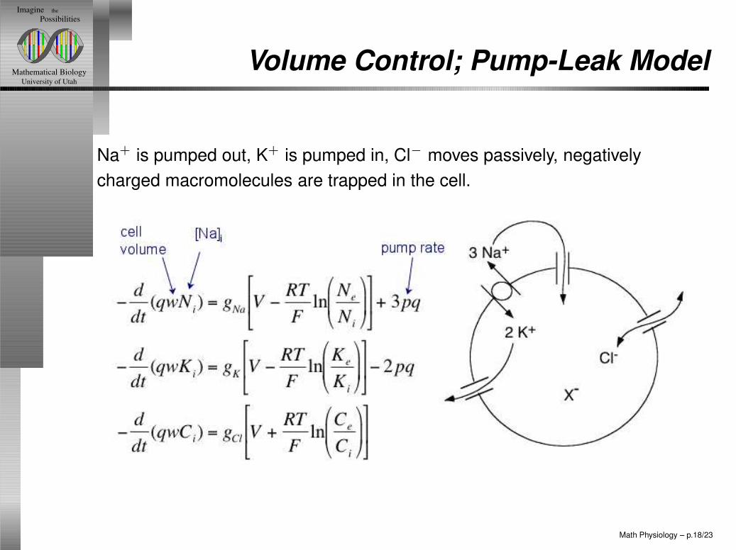
Volume Control; Pump-Leak Model
Na+ is pumped out, K+ is pumped in, Cl− moves passively, negativelycharged macromolecules are trapped in the cell.
Math Physiology – p.18/23
University of UtahMathematical Biology
theImagine Possibilities Charge Balance and Osmotic
Balance
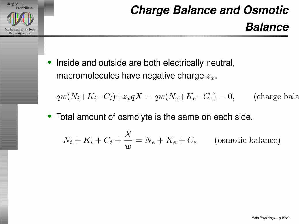
• Inside and outside are both electrically neutral,macromolecules have negative charge zx.
qw(Ni+Ki−Ci)+zxqX = qw(Ne+Ke−Ce) = 0, (charge balance)
• Total amount of osmolyte is the same on each side.
Ni + Ki + Ci +X
w= Ne + Ke + Ce (osmotic balance)
Math Physiology – p.19/23
University of UtahMathematical Biology
theImagine Possibilities
The Solution
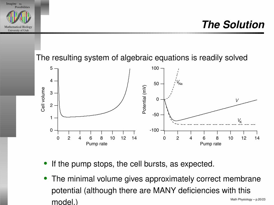
The resulting system of algebraic equations is readily solved5
4
3
2
1
0
Ce
ll vo
lum
e
14121086420
Pump rate
-100
-50
0
50
100
Po
ten
tia
l (m
V)
14121086420
Pump rate
VNa
VK
V
• If the pump stops, the cell bursts, as expected.
• The minimal volume gives approximately correct membranepotential (although there are MANY deficiencies with thismodel.) Math Physiology – p.20/23
University of UtahMathematical Biology
theImagine Possibilities
Volume Control and Ion Transport
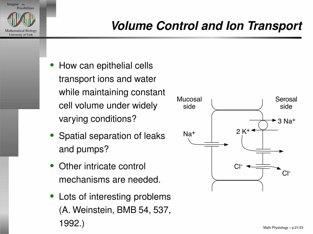
• How can epithelial cellstransport ions and waterwhile maintaining constantcell volume under widelyvarying conditions?
• Spatial separation of leaksand pumps?
• Other intricate controlmechanisms are needed.
• Lots of interesting problems(A. Weinstein, BMB 54, 537,1992.)
3 Na+
2 K+
Mucosal
side
Serosal
side
Na+
Cl-
Cl-
Math Physiology – p.21/23
University of UtahMathematical Biology
theImagine Possibilities
Inner Meduullary Collecting Duct
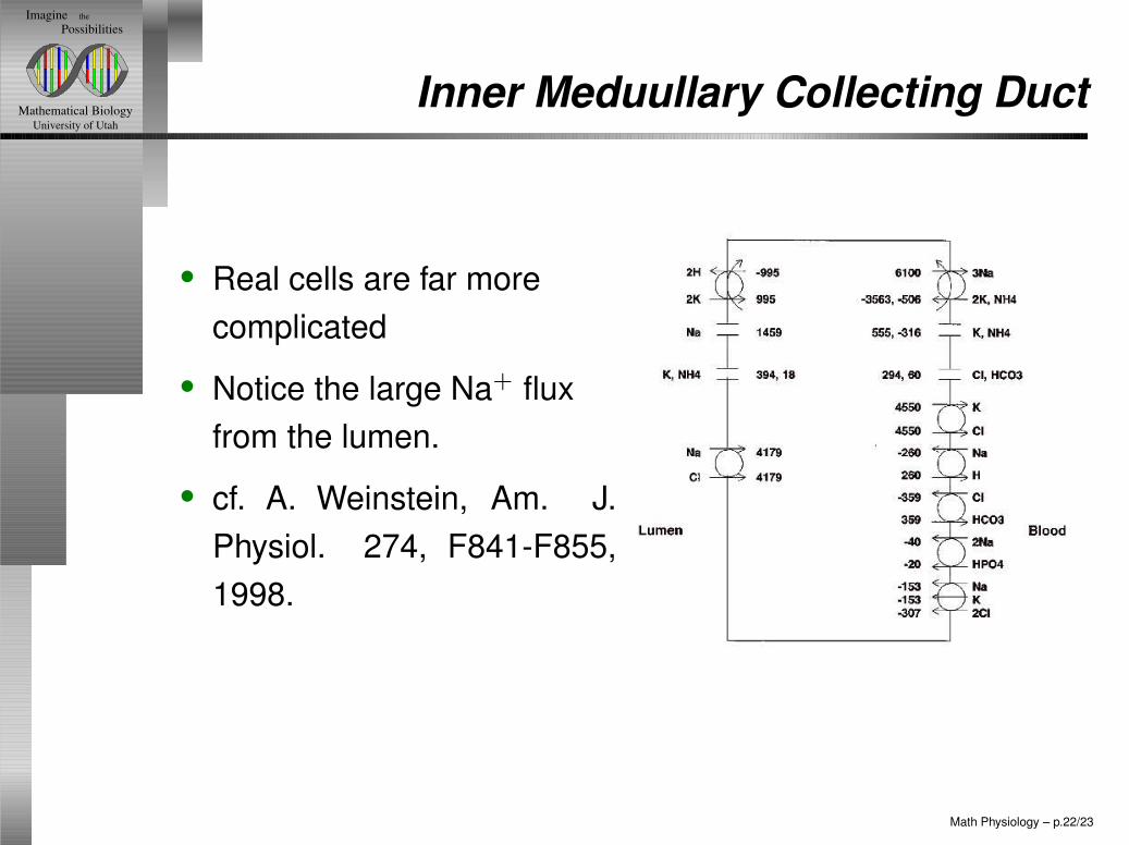
• Real cells are far morecomplicated
• Notice the large Na+ fluxfrom the lumen.
• cf. A. Weinstein, Am. J.Physiol. 274, F841-F855,1998.
Math Physiology – p.22/23
University of UtahMathematical Biology
theImagine Possibilities Interesting Problems (suitable for
projects)
• How do organism (e.g., T. Californicus living in tidal basins)adjust to dramatic environmental changes?
• How do plants in arid, salty regions, prevent dehydration?(They make proline)
• How do fish (e.g., salmon) adjust to both freshwater and saltwater?
• What happens to a cell and its environment when there isischemia (loss of ATP)?
• How do cell in high salt environments (epithelial cell inkidney) maintain constant volume?
Math Physiology – p.23/23