Introduction to R

Contents

1 Hello, R! 2

2 Starting R 2

3 Simple mathematics 33.1 Variables . . . . . . . . . . . . . . . . . . . . . . . . . . . . . . . 43.2 Standard functions . . . . . . . . . . . . . . . . . . . . . . . . . . 5

4 Getting help 6

5 Vectors 75.1 Working with vectors . . . . . . . . . . . . . . . . . . . . . . . . . 8

5.1.1 Entrywise operation on vectors . . . . . . . . . . . . . . . 95.1.2 Summarizing a vector . . . . . . . . . . . . . . . . . . . . 9

5.2 Extracting parts of a vector . . . . . . . . . . . . . . . . . . . . . 105.3 Sorting . . . . . . . . . . . . . . . . . . . . . . . . . . . . . . . . . 12

6 Matrices 136.1 Working with rows and columns . . . . . . . . . . . . . . . . . . 156.2 Vectors are not matrices . . . . . . . . . . . . . . . . . . . . . . . 15

7 Lists 16

8 Meta information 17

9 Functions 179.1 Peeping inside the body of a function . . . . . . . . . . . . . . . . 199.2 Functions returning multiple values . . . . . . . . . . . . . . . . . 209.3 Named arguments . . . . . . . . . . . . . . . . . . . . . . . . . . 209.4 Defaults . . . . . . . . . . . . . . . . . . . . . . . . . . . . . . . . 219.5 Optional arguments . . . . . . . . . . . . . . . . . . . . . . . . . 229.6 Object-orientedness . . . . . . . . . . . . . . . . . . . . . . . . . . 23

10 Control structures 25

11 Packages 26

12 Troubleshooting 27

13 The working directory/folder of R 28

14 File handling 28

1

15 Different ways of running R 3015.1 Script files . . . . . . . . . . . . . . . . . . . . . . . . . . . . . . . 30

16 Running R in batch mode 31

17 Hints for selected exercises 31

1 Hello, R!

R is a free statistical software. It has many uses including

1. performing simple calculations (like a very powerful pocket calculator)

2. making plots (graphs, diagrams etc),

3. analyzing data using ready-made statistical tools (e.g.,, regression),

4. and above all it is a powerful programming language.

We shall acquaint ourselves with the basics of R in this tutorial.

2 Starting R

First you must have R installed in your computer. Then you’ll have to do one ofa number of things depending on your computer set up. The simplest techniqueis to turn to the guy who has worked with R in your lab, and ask for help! Ifno such guy is at hand, then you may try one of these.

• Windows: If you see an icon like then (double) clicking on it shouldwork.

• Linux/Unix: Open a command window (xterm, say) and try typing R.

• Search for the path where R is installed, and navigate to its bin folder.Then run the appropriate executible file in it.

If everything goes well, you should see something like this.

R version 2.13.0 (2011-04-13)

Copyright (C) 2011 The R Foundation for Statistical Computing

ISBN 3-900051-07-0

Platform: i386-pc-mingw32/i386 (32-bit)

R is free software and comes with ABSOLUTELY NO WARRANTY.

You are welcome to redistribute it under certain conditions.

Type ’license()’ or ’licence()’ for distribution details.

2

R is a collaborative project with many contributors.

Type ’contributors()’ for more information and

’citation()’ on how to cite R or R packages in publications.

Type ’demo()’ for some demos, ’help()’ for on-line help, or

’help.start()’ for an HTML browser interface to help.

Type ’q()’ to quit R.

>

The > is the R prompt. You have to type commands in front of this prompt and

press the key on your keyboard.

3 Simple mathematics

R may be used like a simple calculator. Type the following command in front

of the prompt and hit .

2 + 3

[1] 5

Ignore the [1] in the output for the time being. We shall learn its meaninglater. Now try

2 / 3

What about the following? Wait! Don’t type these all over again. Just hit the

key of your keyboard to replay the last line. Now use the and cursor

keys and the key to make the necessary changes.

2 * 3

2 - 3

Exercise 1: What does R say to the following?

2/0

3

Guess the result of

2/Inf

and of

Inf/Inf

�

So now you know about three different types of ‘numbers’ that R can handle:ordinary numbers, infinities, NaN (Not a Number).

3.1 Variables

R can work with variables. For example

x = 4

assigns the value 4 to the variable x. This assignment occurs silently, so you donot see any visible effect immediately. To see the value of x type

x

Here is an important thing to remember: To see the value of the variable just

type its name and hit .Let us create a new variable

y = -4

Try the following.

x + y

x - 2*y

x^2 + 1/y

4

The caret (̂ ) in the last line denotes power.

Exercise 2: What happens if you type the following?

z-2*x

and what about the next line?

X + Y #oops!

�

The part of a line after # is called a comment. It is meant for U, the UseRwho use R! R does not care about comments.

Exercise 3: Can you explain the effect of this?

x = 2*x

�

Unlike many other languages, R allows the dot character (.) as part of a variablename. Thus you can write

speed.light = 3e8 # 3e8 means 3 times 10 to the power 8

3.2 Standard functions

R knows most of the standard functions.

Exercise 4: Try

x=1

sin(x)

cos(0)

sin(pi) #pi is a built-in constant

tan(pi/2)

�

Exercise 5: While you are in the mood of using R as a calculator you may also try

5

exp(1)

log(3)

log(-3)

log(0)

log(x-y)

Can you guess the base of the logarithm? �

4 Getting help

R has many many features and it is impossible to keep all its nuances in one’shead. So R has an efficient online help system. The next exercise introducesyou to this.

Exercise 6: Suppose that you desperately need logarithm to the base 10. You wantto know if R has a ready-made function to compute that. So type

?log

A new window (the help window) will pop up. Do you find what you need? �

Always look up the help of anything that does not seem clear. The techniqueis to type a question mark followed by the name of the thing you are interestedin. All words written like this in this tutorial have online help.Sometimes, you may not know the exact name of the function that you areinterested in. Then you can try the help.search function.

help.search("sin")

It has a simple abbreviation:

??sin

Exercise 7: Can R compute the Gamma function? As your first effort try

Gamma(2) #oops!

Apparently this is not the Gamma function you are looking for. So try

6

help.search("Gamma")

This will list all the topics that involve Gamma. After some deliberation you can seethat “Special Functions of Mathematics” matches your need most closely. So type

?Special

Got the information you needed? �

Searching for functions with names known only approximately is often frustrat-ing.Usually it is easier to google the internet than perform help.search!

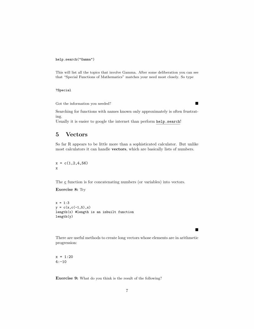
5 Vectors

So far R appears to be little more than a sophisticated calculator. But unlikemost calculators it can handle vectors, which are basically lists of numbers.

x = c(1,2,4,56)

x

The c function is for concatenating numbers (or variables) into vectors.

Exercise 8: Try

x = 1:3

y = c(x,c(-1,5),x)

length(x) #length is an inbuilt function

length(y)

�

There are useful methods to create long vectors whose elements are in arithmeticprogression:

x = 1:20

4:-10

Exercise 9: What do you think is the result of the following?

7

n = 10

1:n+1

�

If the common difference is not 1 or −1 then we can use the seq function

y=seq(2,5,0.3)

y

Exercise 10: Try the following

1:100

Do you see the meaning of the numbers inside the square brackets? �

Exercise 11: How to create the following vector in R without typing out the entirelist?

1, 1.1, 1.2, , ... 1.9, 2, 2, 1.9, 1.8, ... 1.1, 1

�

The rep function is another useful thing to know:

rep(1,10) #a vector of 1’s having length 10

rep(1:3,10) #1,2,3, 1,2,3, 1,2,3,...ten times

5.1 Working with vectors

Now that we know how to create vectors in R, it is time to use them. There arebasically three different types of functions to handle vectors.

1. those that work entrywise

2. those that summarize a vector into a few numbers (like summing all thenumbers)

3. others

8

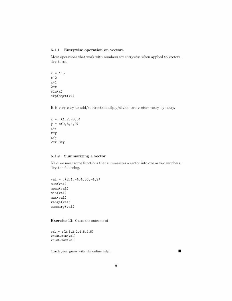
5.1.1 Entrywise operation on vectors

Most operations that work with numbers act entrywise when applied to vectors.Try these.

x = 1:5

x^2

x+1

2*x

sin(x)

exp(sqrt(x))

It is very easy to add/subtract/multiply/divide two vectors entry by entry.

x = c(1,2,-3,0)

y = c(0,3,4,0)

x+y

x*y

x/y

2*x-3*y

5.1.2 Summarizing a vector

Next we meet some functions that summarizes a vector into one or two numbers.Try the following.

val = c(2,1,-4,4,56,-4,2)

sum(val)

mean(val)

min(val)

max(val)

range(val)

summary(val)

Exercise 12: Guess the outcome of

val = c(2,3,2,2,4,5,2,5)

which.min(val)

which.max(val)

Check your guess with the online help. �

9

5.2 Extracting parts of a vector

If x is a vector of length 3 then its entries may be accessed as x[1], x[2] and x[3].Note that the counting starts from 1 and proceeds left-to-right. The quantityinside the square brackets is called the subscript or index. C/C++ and Javausers beware: indexing in R starts from 1, and not from 0.

x = c(2,4,-1)

x[1]

x[2]+x[3]

i = 3

x[i]

x[i-1]

x[4]

It is also possible to access multiple entries of a vector by using a subscript thatis itself a vector.

x = 3:10

x[1:4]

x[c(2,4,1)]

What is the effect of the following?

x = c(10,3,4,1)

ind = c(3,2,4,1) #a permutation of 1,2,3,4

x[ind]

This technique is often useful to rearrange a vector.

Exercise 13: Try the following to find how R interprets negative subscripts.

x = 3:10

x

x[-1]

x[-c(1,3)]

�

Exercise 14: Does R allow fractional subscripts? Find out using the following lines.

10

x = 10:20

x[3.9]

�

Subscripting allows us to find one or more entries in a vector if we know the po-sition(s) in the vector. There is a different (and very useful) form of subscriptingthat allows us to extract entries with some given property.

x = c(100,2,200,4)

x[x>50]

The second line extracts all the entries in x that exceed 50. There are somenifty things that we can achieve using this kind of subscripting. To find thesum of all entries exceeding 50 we can use

sum(x[x>50])

How does this work? If you type

x>50

you will get a vector of TRUEs and FALSEs. A TRUE stands for a case where theentry exceeds 50. When such a TRUE-FALSE vector is used as the subscript onlythe entries corresponding to the TRUEs are retained:

x[c(T,T,F,T)] #T means TRUE, F means FALSE

Even that is not all. Internally a TRUE is basically a 1, while a FALSE is a 0. Soif you type

sum(x>50)

you will get the number of entries exceeding 50.The number of entries satisfying some given property (like “less than 4”)maybe found easily like

11

sum(x<4)

Exercise 15: If

val = c(1,30,10,24,24,30,10,45)

then what will be the result of the following?

sum(val >= 10 & val <= 40)

sum(val > 40 | val < 10) # | means "OR"

sum(val == 30) #we are using == and not =

sum(val != 24)

Be careful with ==. It is different from =. The former means comparing for equality,

while the latter means assignment of a value to a variable. �

Exercise 16: What does

mean(x>50)

compute? No, it is not the mean of all the x’s exceeding 50. �

Exercise 17: Try and interpret the results of the following.

x = c(100,2,200,4)

sum(x>=4)

mean(x!=2)

x==100

mean(x[x>500]) #Oops!

�

5.3 Sorting

x = c(2,3,4,5,3,1)

y = sort(x)

y #sorted

x #unchanged

12

Exercise 18: Look up the help of the sort function to find out how to sort in

decreasing order. �

Sometimes we need to order one vector according to another vector.

x = c(2,3,4,5,3,1)

y = c(3,4,1,3,8,9)

ord = order(x)

ord

Notice that ord[1] is the position of the smallest number, ord[2] is the positionof the next smallest number, and so on.

x[ord] #same as sort(x)

y[ord] #y sorted according to x

6 Matrices

R has no direct way to create an arbitrary matrix. You have to first list all theentries of the matrix as a single vector (an m by n matrix will need a vector oflength mn) and then fold the vector into a matrix. To create[

1 23 4

]we first list the entries column by column to get

1, 3, 2, 4.

To fold it into a matrix:

A = matrix(c(1,3,2,4),nrow=2)

A

The nrow=2 command tells R that the matrix has 2 rows (then R can computethe number of columns by dividing the length of the vector by nrow.) You couldhave also typed the following.

A <- matrix(c(1,3,2,4),ncol=2) #<- is same as =

13

Some people prefer to use ‘<-’ instead of ‘=’ to assign values to a variable. Formost purposes they are equivalent, except that the former requires extra typing.Also be careful about the distinction between x < -1 and x<-1.Notice that R folds a vector into a matrix column by column. Sometimes,however, we may need to fold row by row :

A = matrix(c(1,3,2,4),nrow=2,byrow=T)

The T is same as TRUE.

Exercise 19: Matrix operations in R are more or less straight forward. Try thefollowing.

A = matrix(c(1,3,2,4),ncol=2)

B = matrix(2:7,nrow=2)

C = matrix(5:2,ncol=2)

dim(B) #dimension

nrow(B)

ncol(B)

A+C

A-C

A%*%C #matrix multiplication

A*C #entrywise multiplication

A%*%B

t(B)

�

Subscripting a matrix is done much like subscripting a vector, except that for amatrix we need two subscripts. To see the (1,2)-th entry (i.e., the entry in row1 and column 2) of A type

A[1,2]

Exercise 20: Try out the following commands to find what they do.

A[1,]

B[1,c(2,3)]

B[,-1]

�

14

6.1 Working with rows and columns

Consider the following.

A = matrix(c(1,3,2,4),ncol=2)

sin(A)

Here the sin function applies entrywise. Now suppose that we want to find thesum of each column. So we want to apply the sum function columnwise. Weachieve this by using the apply function like this:

apply(A,2,sum)

The 2 above means columnwise. If we need to find the rowwise means we canuse

apply(A,1,mean)

6.2 Vectors are not matrices

This is a jolt to Matlab users, and is the cause of many a trouble in R. SometimesR treats a vector as a (row/column) matrix, sometimes not.

x = 1:3 #a vector

A = matrix(1:9,3,3) #a matrix

A %*% x #x is treated as a column vector

x %*% A #x is treated as a row vector

Let’s check the dimension using the dim function:

dim(A)

dim(x)

The as.matrix function converts a vector to a column matrix.

x1 = as.matrix(x)

dim(x1)

15

Here is an example to show how the confusion between vectors and matricesmay lead to trouble. The diag function has two purposes:

• when applied to matrices it extracts the diagonal entries

• when applied to vectors, it creates a diagonal matrix.

Try out the following and see the difference.

diag(A)

diag(x)

diag(x1)

Exercise 21: Now try to guess the output of the following.

x = 1:2

A = matrix(1:4,2,2)

diag(A %*% x)

�

7 Lists

Vectors and matrices in R are two ways to work with a collection of objects.Lists provide a third method. Unlike a vector or a matrix a list can holddifferent kinds of objects. Thus, one entry in a list may be a number, while thenext is a matrix, while a third is a character string (like ”Hello R!”). Lists areuseful to store different pieces of information about some common entity. Thefollowing list, for example, stores details about a student.

x = list(name="Chang", nationality="Chinese",

height=5.5, grades=c(95,45,80))

We can now extract the different fields of x as

names(x)

x$name

x$hei #abbrevs are OK

x$grades

x$g[2]

x$na #oops!

16

Lists are useful in R because they allow R functions (we shall learn about themsoon) to return multiple values.Most statistical functions in R usually return their results in the form of lists.So we must know how to unpack a list using the $ symbol as above.To see the online help about symbols like $ type

?"$"

Notice the quotes surrounding the symbol.

8 Meta information

An interesting feature of R is that allows arbitrary meta-information to be as-sociated with any variable. These are called attributes. For example, supposethat we have a vector x

x = 1:10

and we want to associate an attribute date with it. Then we shall use

attr(x,’date’) = "June 6, 2011"

You may find the attributes associated with an object using the attributes

function:

attributes(x) #Looking up all attributes.

attr(x,’date’) #Looking up a specific attribute.

Certain attributes are special and are used internally by R. One such is the dim

attribute that stores the dimension of an array. A 3 × 4 matrix in R is, forinstance, nothing but a vector of length 12, along with an attribute dim equalto (3, 4).

9 Functions

We can type

sin(1)

17

to get the value sin(1). Here sin is a standard built-in function. R allows us tocreate new functions of our own. For example, suppose that some computationrequires you to find the value of

f(x) = x/(1− x)

repeatedly. Then we can write function to do this as follows.

f = function(x) x/(1-x)

Here is an more elaborate but equivalent form:

f = function(x) {

x/(1-x)

}

The braces are compulsory for functions with more than one line. By default afunction returns the value of the very last line executed. So one does not have tomention return explicitly. But the following form is also allowed. In R return

is a function, and so the parentheses after it are compulsory.

f = function(x) {

return( x/(1-x) )

}

Once f is defined you may type things like

f(2)

y = 4

f(y)

f(2*y)

Here f is the name of the function. It can be any name of your choice (as longas it does not conflict with the keywords.

Anatomy of an R function

18

A couple of points are in order here. First, the choice of the name dependscompletely on you. Second, the name of the argument is also a matter ofpersonal choice. But you must use the same name also inside the body of thefunction.It is also possible to write functions of more than one variable.

Exercise 22: Try out the following.

g = function(x,y) (x+2*y)/3

g(1,2)

g(2,1)

�

Exercise 23: Write a function with name myfun that computes x + 2y/3. Use it to

compute 2 + 2 × 3/3. �

Exercise 24: Consider the trivial function

f = function(x,y) x+2*y

Now try out the following and explain the output.

f(1:2,2:3)

f(1:4,2:3) #The two input vectors are of different lengths!

f(1:4,1:5) #Oops!

�

9.1 Peeping inside the body of a function

Sometimes you may be curious as to how a certain function is implemented.A simple way to peep inside the definition of a function is to type the nameof the function (sans any parentheses or arguments) at the command prompt,

and hit . The entire body of the function will be listed on screen.While the output will often be overwhelmingly long (and somewhat cryptic), itis nevertheless a great way to learn new R programming tricks. The functioncov computes covariances. Type

cov

to get a feel for what goes inside its body!

19

9.2 Functions returning multiple values

An R function is allowed to return only a single R object. Sometimes we needfunctions computing more than one value. Then lists come in handy.Suppose that we want to write a function that finds the length, total and meanof a vector. Since the function is returning three different pieces of informationwe should use lists.

f = function(x) list(len=length(x),total=sum(x),mean=mean(x))

Now we can use it like this:

dat = 1:10

result = f(dat)

names(result) #a sneak peek into the returned list

result$len

result$tot

result$mean

9.3 Named arguments

It is not uncommon for an R function to have a large number of parameters.It is difficult to remember the order of the parameters of such functions. Thenone can use named arguments. Consider, for example,

f = function(x,y,z) {

cat("x = ",x," y = ",y," z = ",z,"\n")

}

See the difference in the effects of the following two lines.

f(1,2,3)

f(y=1,x=2,z=3)

The name of an argument may be abbreviated as long as there is no ambiguity.Consider the following function.

f = function(maxval, minval, mintol)

cat("maxval = ",maxval," minval = ",minval," mintol = ",mintol,"\n")

20

The cat function is a output function that can print a sequence objects in anunformatted way (unlike print that prints a single object in a formatted way).Now try

f(max=10, minv=1, mint = 5)

f(max=10, min=1, mint = 5) #oops!

9.4 Defaults

Like many other softwares, R tries to be scalable. This means that it triesto allow simple things to be done simply and yet keep the provision open foradding complexity for more detailed output. One mechanism to achieve this isby allowing function parameters to have default values. Most sophisticated Rfunctions have a long list of parameters with default values. These parametersremain transparent to a novice user, and yet allow advanced users to fine tunethe computation. Here is an example.

f = function(x,y,z=3) {

cat("x = ",x," y = ",y," z = ",z,"\n")

}

Now try

f(1,2,3)

f(1,2)

f(y=5,x=2)

f(x=4) #oops!

Exercise 25: Consider

g = function(x,y=2,z)

cat("x = ",x," y = ",y," z = ",z,"\n")

}

What will the command

g(1,3)

21

produce? How can you call the function with x and z equal to 1 and 3, respectively,

and using the default value for y? �

A default value can be an expression also as shown next.

f = function(x, y=x+2*z, z) {

cat("x = ",x," y = ",y," z = ",z,"\n")

}

Try

f(1,z=2)

To see it in action.

9.5 Optional arguments

An R function can call other R functions. A common situation is where astatistical function needs to call the plot function to plot something. As maybe guessed, the plot function has a large number of parameters (with defaultvalues for most) to provide fine control over the plot. Now the user of thestatistical function may want to play with these plotting parameters. In such ascenario the statistical function provides direct access to the plotting parametersby using optional parameters.In order to understand the following example, just remember that the two vari-ants of the plot command1.

plot(x,y) #makes a scatterplot of (xi,yi)’s

plot(x,y,col=’red’) #same thing, but red in color

Now consider an example with optional parameters (denoted by the ellipsissymbol).

statFun = function(x,y,...) {

#Do whatever analysis you want, eg, compute

#the following two new variables, say.

newX = 2*x

newY = x+y

plot(newX,newY,...)

}

1We shall talk more about plotting later.

22

Now try the following.

statFun(1:10,3:13)

statFun(1:10,3:13,col=’red’)

9.6 Object-orientedness

R has a simple object-oriented structure, that allows the ”same” function tobehave differently for different classes of the first argument. One example isthe summary function.

x = 1:12

summary(x)

y = matrix(x,3,4)

summary(y)

To see the reason behind the difference in behavior let’s look at the classes ofx and y.

class(x)

class(y)

By the way, class is just an attribute. So the last line could also be written as

attr(y,’class’)

Now, the summary function is just a wrapper. Behind the screen there are two2

functions called summary.matrix and summary.default. For an object of classmatrix the function that actually gets invoked is summary.matrix. Notice thestructure of the name:

name of wrapper . name of class

Now there is no function called summary.numeric, so the call summary(x) ex-pands into summary.default(x).Throughout this course we shall encounter many different classes, and such“overloaded” functions. So it will help to familiarize ourselves with this mech-anism.

2In fact, many more

23

Suppose that we want to have a function area that will compute area of botha rectangle as well as a circle. We shall specify a rectangle in terms of thecoordinates of a pair of diagonally opposite corners(x1, y1), (x2, y2). A circle will be represented by the center (x, y) and the radiusr.First we create the wrapper.

area = function(shape) {

UseMethod("area")

}

Now let us create two work horse functions.

area.circle = function(shape) pi * shape$r^2

area.rect = function(shape) abs((shape$x1-shape$x2) * (shape$y1-shape$y2))

It is a good idea to create a default function, which in our case does nothingbut produce an error message.

area.default = function(shape) stop("Not a known shape")

Now let us put these to use.

x = list(x1=3,y1=5,x2=4,y2=10)

class(x) = "rect"

y = list(x=3,y=5,r=4)

class(y) = "circle"

area(x)

area(y)

area(1:10) #oops!

By the way you can also use the “expanded” form

area.circle(y)

area.rect(x)

area.rect(y) #oops!

24

Thus the same function name may correspond to multiple definitions, one foreach class (plus one default). One may be interested in knowing a list of all thedefinitions corresponding to the same function name. The function methods

allows us to query just that!

methods(area)

methods(summary)

Sometimes we want to make the opposite query: How many functions are therefor a given class? Again the methods function comes to the rescue.

methods(class="matrix")

10 Control structures

R is a powerful programming language, and has the standard control structureslike loops and conditional jumps. In this course, we shall make only sparing useof the advanced programming features of R, but here are some simple examplesfor the interested readers.

for(i in 1:10) {

if(i < 5) {

print("Small")

}

else {

print("Large")

}

}

Incidentally, loops like the above are pretty slow in R, and are often avoided bynifty tricks. The above code for example can be reduced to the more efficientline using the ifelse function:

ifelse((1:10)<5, "Small", "Large")

Another nifty trick for avoiding explicit loops is the sapply function, which weshall learn to use once we later. It applies a function to the elements of a vector:

25

f = function(x) print("Hello")

x = sapply(1:5, f)

We can even abbreviate to

x = sapply(1:5, function(x) print("Hello"))

Here we see an example of an anonymous function.We shall learn more about these tricks as and when we shall use them.

11 Packages

The R software may be considered as made of two parts. The core and the extrapackages. The core is what you install when you install R3. The extra packages(and there are many, the count increasing by the day) may be added as andwhen needed. This package mechanism gives R its true power.A package is nothing but a collection of R functions and data sets, along withsome documentation, neatly arranged in a standardized format. Any one cancreate a package and make it available to fellow users over the internet. Indeed,there is a h..u..g..e web repository of R packages called the The Comprehen-sive R Archive Network (CRAN) at http://cran.r-project.org/As we shall be spending a large amount to time working with downloaded pack-ages, let us familiarize ourselves with the usage.There are four steps to use a package:

1. find the name of the package (Google is a great help here!)

2. download it (typically as a .tar.gz file)

3. install it

4. load it into an R session.

The first three steps are to be done only once. The last step needs to be donefor each R session using that package. Once you learn the name of a package(say zyp) with some functionality you want, you type the following at the Rprompt.

install.packages(’zyp’) #Quotes (single/double) are must!

3Actually, a few standard packages also get installed by default.

26

Assuming that you have an active internet connection, this will prompt youto choose a mirror (the CRAN is spread over mirror sites all throughout theglobe). Once you choose a mirror, the download will start, and the packagewill get installed automatically. If the package requires some other packagenot already installed in your system then those will also be downloaded andinstalled.In order to load the installed package you use the library function.

library(zyp) #You may or may not use quotes.

12 Troubleshooting

Any software is prone to bugs, and a software like R that relies on textual inputfrom the user (as opposed to point-n-click), typos can wreak havoc. Unfortu-nately, the default error mechanism of R is rather crude and produces crypticerror messages. Let’s see an example

f = function(day,tempInC) {

tempInF = 32+1.8*tempInC

plot(day,tempInF)

}

Consider using it as

f(1:10,1:11) #oops!

R complains:

Error in xy.coords(x, y, xlabel, ylabel, log) :

’x’ and ’y’ lengths differ

You’ll get a rather cryptic error message involving names that you have possiblynever heard of! Fortunately R has a smarter debugging facility that we shownext.

options(error=quote(dump.frames("testdump"))) #preparing to trap bugs

#code to be debugged

f(1:10,1:11) #oops!

options(error=NULL) #close the trap

debugger(testdump) #inspect

27

13 The working directory/folder of R

During its course of action R has to often handle files (e.g., reading data/commands,writing output). In any operating system files are stored hierarchically in direc-tories/folders. R treats one of these folders as its working directory. You cansee it by the command

getwd() #get working directory

By default R will read files from this folder, and files created by R will reside inthis folder. We can of course change the default folder using the setwd function:

#You may use ’/’ in any operating system

setwd("c:/whatever/path/you/want")

#’$\backslash$’ only for Windows

setwd("c:$\backslash$whatever$\backslash$path$\backslash$you$\backslash$want")

It is also possible to use relative paths like

setwd("..") #parent directory

In a Windows machine the default folder may be selected via the File menu aswell. When you run R in a Penn State lab machine, the initial default directoryis somewhere that you do not have write access to. So you will need the followingcommand:

setwd(’v:/Desktop’)

14 File handling

There are two aspects to file handling in R: writing and reading. The highestlevel output function is print. It prints any R output in a formatted way onthe screen. We can redirect the output to a file using the sink command.

x = matrix(1:12,3,4) # Some R object

sink(’myfile.txt’) # redirecting the output

summary(x) #Nothing is printed on screen

sink() #redirecting output back to screen

28

If we want finer control on what we want to print then we can use the low levelfunction cat:

y = 20

cat("The answer is",y,"\n",file="myfile.txt")

cat("This is a second line\n",file="myfile.txt",append=T)

If we want to dump the value of an R object in a human readable way then thewrite function comes handy.

x = matrix(1:12,3,4)

write(x,ncol=4,file=’myfile.txt’)

Exercise 26: What is difference between the following two lines? Read the onlinehelp to find out.

write(x)

write(x,file=’’)

�

But if our sole aim is to dump the value of an R object to be read back in afuture session then the simplest way is to use the save and load functions.

save(x,file=’abc’)

Now let’s delete the object x:

rm(x)

x #Oops!

Now we shall reload it from the file:

load(’abc’)

x #It’s back!

R allows reading data in many different formats. We shall discuss them in thenext tutorial.

29

15 Different ways of running R

15.1 Script files

So far we are using R interactively where we type commands at the prompt andthe R executes a line before we type the next line. But sometimes we may wantto submit many lines of commands to R at a single go. Then we need to usescripts.Use script files to save frequently used command sequences. Script files are alsouseful for replaying an analysis at a later date.A script file in R is a text file containing R commands (much as you wouldtype them at the prompt). As an example, open a text editor (e.g., notepad inWindows, or gedit in Linux). Avoid fancy editors like MSWord. Create a filecalled, say, test.r containing the following lines.

x = seq(0,10,0.1)

y = sin(x)

plot(x,y,ty="l")

Save the file in some folder (say F:\astro).In order to make R execute this script type

source("F:/astro/test.r") #We are specifying the entire path.

#So no need to care about default

#folder.

In this as well as other examples involving files, you must use the actual path onyour system for things to work. The examples give the paths that work in mymachine. If your script has any mistake in it then R will produce error messagesat this point. Otherwise, it will execute your script.The variables x and y created inside the command file are available for use fromthe prompt now. For example, you can check the value of x by simply typingits name at the prompt.

x

Commands inside a script file are executed pretty much like commands typedat the prompt. One important difference is that in order to print the value ofa variable x on the screen you have to write

print(x)

30

Merely writing

x

on a line by itself will not do inside a script file.Printing results of the intermediate steps using print from inside a script fileis a good way to debug R scripts.

16 Running R in batch mode

Let us first create a script file called test.r containing the following lines. Keepthe file on your desktop.

cat("It works!\n") #cat simply prints its arguments without

#any embellishment.

x = 1:100

print(x)

Now open a command prompt, navigate to your desktop folder and type

17 Hints for selected exercises

2. Well, I should have told you already: R is case sensitive!3. The value of x gets doubled.

31

4. tan π2 is actually undefined. But R cannot store π

2 exactly. R’s representa-tion of π

2 happens to be a bit less than π2 . So tan(pi/2) becomes a very large

number.5. Natural logarithm.8. length(x) is 3, and length(y) is 8.9. Same as 2:11. So use 1:(n+1) if we want to have 1:11.10. They are actually the indices of the first numbers in each line.11. We may use c(10:20,20:10)/10 or use the rev function x=seq(1,2,0.1);

c(x,rev(x))

12. The position of the first occurrence of minimum or maximum.13. The corresponding entries are suppressed. They are not deleted from theoriginal vector, by the way!14. x[3.9] is the same as x[3]. Thus x[a] is the same as x[floor(a)].16. The proportion of elements greater than 50. To find the mean of all thex’s greater than 50, you need mean(x[x>50]).18. sort(x,decreasing=T)

20. B[,-1] means B without its first column.21. R treats A %*% x as a matrix, and so diag extracts its diagonal element,which happens to be 7. If, instead, we wanted to have a 2× 2 diagonal matrixwith diagonal given by the vector A %*% x, we should use

diag(as.vector(A %*% x))

23. f = function(x,y) x+2*y/3. Don’t forget the *!24. A function automatically applied entrywise on vectors. Shorter vectorsare recycled to match the longer one. Warning is issued if fractional number ofrecycling is required.25. Error, since the value 1 goes to x, 2 goes to y, but z gets no value, andhas no default! g(x=1,z=3) or g(1,z=3) will both work.26. write(x) writes x to a file called data in the default folder. The otherline dumps x on the screen.

32