Inventory Management

Lecture Outline

• Elements of Inventory Management

• Inventory Control Systems

• Economic Order Quantity Models

• Quantity Discounts

• Reorder Point

• Order Quantity for a Periodic Inventory System

What Is Inventory?

• Stock of items kept to meet future demand

• Purpose of inventory management

• how many units to order

• when to order

Importance of Inventory

• Balance the advantages and

disadvantages of small and large

inventories

• Pressures for small inventories

• Inventory holding cost

• Cost of capital

• Storage and handling costs

• Taxes, insurance, and shrinkage

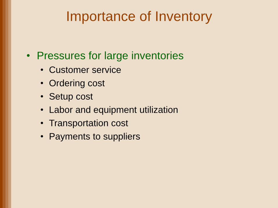
Importance of Inventory

• Pressures for large inventories

• Customer service

• Ordering cost

• Setup cost

• Labor and equipment utilization

• Transportation cost

• Payments to suppliers

Reasons for Holding Inventory

• To meet anticipated customer demand

• To protect against stock outs

• To take advantage of economic order cycles

• To maintain independence of operations

• To allow for smooth and flexible production

operations

• To guard against price increases

In Short,

Buffer against uncertainty in…..

Supply (Raw material inventories)

Production process ( Work in process inventories)

&

Demand (Finished good inventories)

Supply Chain Management

• Bullwhip effect• demand information is distorted as it moves away

from the end-use customer

• higher safety stock inventories to are stored to compensate

• Seasonal or cyclical demand

• Inventory provides independence from vendors

• Take advantage of price discounts

• Inventory provides independence between stages and avoids work stoppages

Inventory Management

To have the correct inventory at the right place at

the right time to minimize system costs while

satisfying customer service requirements

•Raw material/WIP/Finished goods

Inventory Policy

The strategy, approach, or set of techniques used to determine how to manage inventory

Quality Management in the Supply Chain

• Customers usually perceive quality service as

availability of goods they want when they want

them

• Inventory must be sufficient to provide high-

quality customer service in QM

Type of Inventory

Process

stage

Demand

TypeOthers

Raw Materials

WIP

Finished Goods

Independent

Dependent

Spares

Consumable

Purpose

Cycle

Safety

Seasonal

Pipeline

Independent Demand(demand for item is independent

of demand for any other item)

Dependent Demand(demand for item is dependent

upon the demand for some

other item)

Independent vs. Dependent Demand

Independent vs. Dependent Demand..

ItemMaterials With

Independent Demand

Materials With

Dependent Demand

Demand

SourceCompany Customers Parent Items

Material

TypeFinished Goods WIP & Raw Materials

Method of

Estimating

Demand

Forecast & Booked

Customer Orders

Calculated

Planning

MethodEOQ & ROP MRP

Inventory Type : Purpose

• Seasonal stocks– These are accumulated to absorb seasonal fluctuations in

supply or demand.

• Cycle stocks– Due to fixed transportation and handling charges or set up

requirements, it is economical to order or produce largequantities at a time.

• Safety stocks– These are built as a hedge against uncertainties in supply or

demand.

• Pipeline stocks– Inventories in-transit.

Inventory Costs

• Carrying cost

• cost of holding an item in inventory

• Ordering cost

• cost of replenishing inventory

• Shortage cost

• temporary or permanent loss of sales when

demand cannot be met

What are these costs made of? How to estimate these?

Terms used in Inventory

• Material cost = Ci (Average price paid per unit purchased is a key cost in the lot-

sizing decision )

• Fixed ordering cost = Co (Fixed ordering cost includes all costs that do not vary

with the size of the order but are incurred each time an order is placed)

• Holding cost = CH = %*Ci (Holding cost is the cost of carrying one unit in

inventory for a specified period of time i.e. $ CH/Unit/Year)

• Quantity in a lot or batch size = Q (Quantity is either produced or purchased at

a time, EOQ* = Q* )

• Demand per unit time = D (i.e. Demand in one 1 year, d = average demand per

week, So, D = d *52 / year)

Inventory Cost

Holding Costs (CH)

• Obsolescence

• Insurance

• Extra staffing

• Interest

• Pilferage

• Damage

• Warehousing

• etc.

Ordering Costs (Co)

• Supplies

• Forms

• Order processing

• Clerical support

• etc.

• Clean-up costs

• Re-tooling costs

• Adjustment costs

• etc.

Setup Costs (Cs)

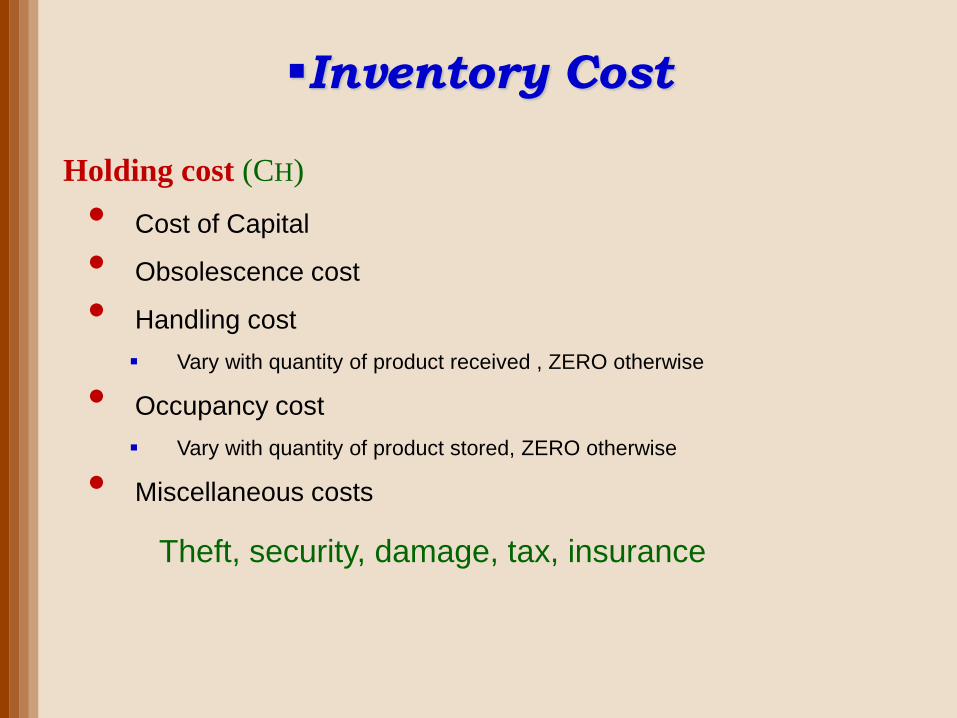
Holding cost (CH)

• Cost of Capital

• Obsolescence cost

• Handling cost

Vary with quantity of product received , ZERO otherwise

• Occupancy cost

Vary with quantity of product stored, ZERO otherwise

• Miscellaneous costs

Theft, security, damage, tax, insurance

Inventory Cost

Ordering cost (Co)

• Buyer time

Time of buyer for placing extra order, ZERO otherwise

Internet and communication has reduced this cost significantly

• Receiving costs

Administrative work such as purchase order matching with updating

inventory records

Quantity dependent should not be included here

• Transportation costs

Fixed cost should be included here

Inventory Cost

Shortage Costs

When occurs, company faces two

possibilities…..

• It can meet the shortage with some type

of rush, special handling or priority

shipment

• It cannot meet the shortage at all

So…. It depends on

How company handles the problem ?

• Permanent– Lost profits due to unsatisfied demand

– Lost profits of future sales

• Temporary (CB)– Backordered, so not necessarily lost

– Special clerical & paperwork costs

– Extraordinary transportation cost to cutomer

Shortage Costs

Inventory policy considerations:

• Customer demand: known/random

• Replenishment lead time: known/random

• Product variety (# of SKUs)

• Length of planning horizon

• Costs: Order costs Vs Inventory costs

• Service level requirements

Inventory management policies/ control

systems:

• Periodic review policy• No tracking of inventory position on a regular basis.

• Inventory position is reviewed after a fixed period,

• Based on a pre-specified order up to level the firm decides the order size.

• Continuous review policy• As soon as the inventory position goes down a certain pre-

specified level the order is placed.

Since most firms have real time inventory information systems in place, the continuous review policy would be the focus.

ABC Analysis

• Stock-keeping units (SKU)

• Identify the classes so management can

control inventory levels

• A Pareto chart

ABC Classification

• Class A

• 5 – 15 % of units

• 70 – 80 % of value

• Class B

• 30 % of units

• 15 % of value

• Class C

• 50 – 60 % of units

• 5 – 10 % of value

ABC Classification

1 $ 60 90

2 350 40

3 30 130

4 80 60

5 30 100

6 20 180

7 10 170

8 320 50

9 510 60

10 20 120

PART UNIT COST ANNUAL USAGE

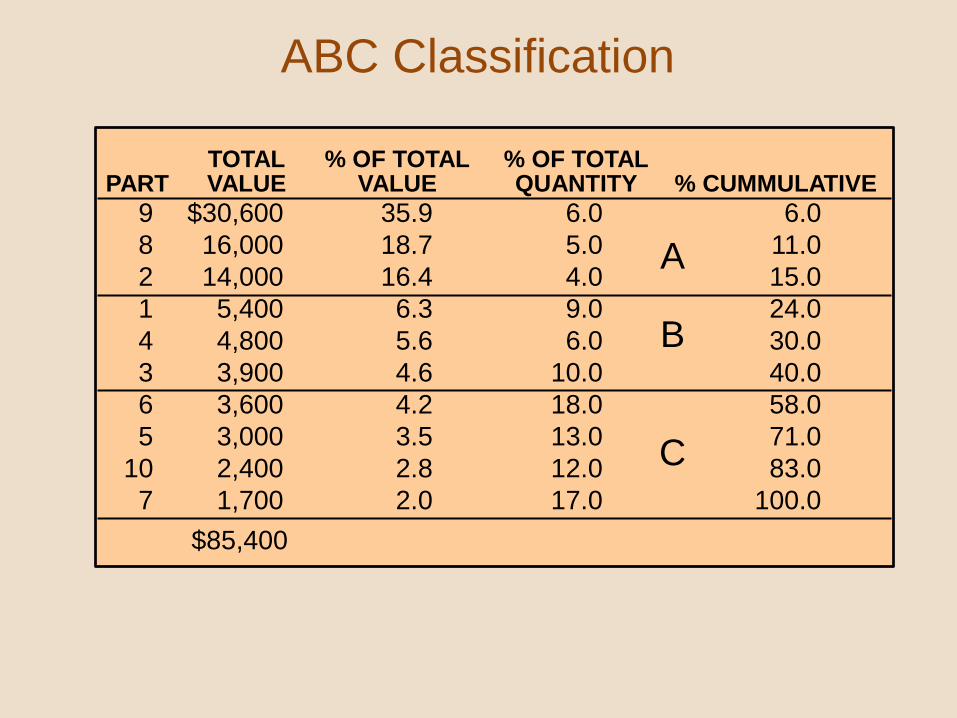
ABC Classification

9 $30,600 35.9 6.0 6.0

8 16,000 18.7 5.0 11.0

2 14,000 16.4 4.0 15.0

1 5,400 6.3 9.0 24.0

4 4,800 5.6 6.0 30.0

3 3,900 4.6 10.0 40.0

6 3,600 4.2 18.0 58.0

5 3,000 3.5 13.0 71.0

10 2,400 2.8 12.0 83.0

7 1,700 2.0 17.0 100.0

TOTAL % OF TOTAL % OF TOTALPART VALUE VALUE QUANTITY % CUMMULATIVE

A

B

C

$85,400

ABC Classification

% OF TOTAL % OF TOTALCLASS ITEMS VALUE QUANTITY

A 9, 8, 2 71.0 15.0

B 1, 4, 3 16.5 25.0

C 6, 5, 10, 7 12.5 60.0

ABC Problem

Booker’s Book Bindery divides SKUs into three classes, according to their dollar usage.

Calculate the usage values of the following SKUs and determine which is most likely to be classified as class A.

SKU Number DescriptionQuantity Used

per YearUnit Value

($)

1 Boxes 500 3.00

2 Cardboard (square feet)

18,000 0.02

3 Cover stock 10,000 0.75

4 Glue (gallons) 75 40.00

5 Inside covers 20,000 0.05

6 Reinforcing tape (meters)

3,000 0.15

7 Signatures 150,000 0.45

Economic Order Quantity

(EOQ) Models

• EOQ

• optimal order quantity that will minimize

total inventory costs

• Basic EOQ model

• Production quantity model

Assumptions of Basic EOQ Model

• Demand is known with certainty and is constant over time

• No shortages are allowed

• Lead time for the receipt of orders is constant

• Order quantity is received all at once

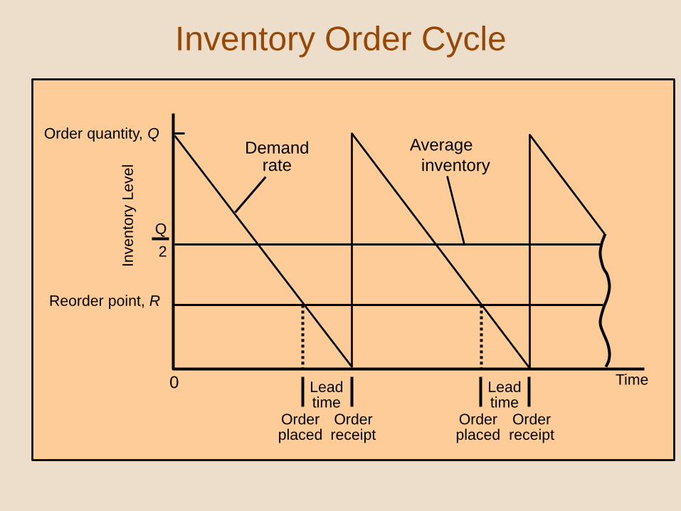
Inventory Order Cycle

Demand rate

TimeLead time

Lead time

Order placed

Order placed

Order receipt

Order receipt

Invento

ry L

evel

Reorder point, R

Order quantity, Q

0

Average

inventory

Q

2

EOQ Cost Model

Co - cost of placing order D - annual demand

Cc - annual per-unit carrying cost Q - order quantity

Annual ordering cost =CoD

Q

Annual carrying cost =CcQ

2

Total cost = +CoD

Q

CcQ

2

EOQ Cost Model

TC = +CoD

Q

CcQ

2

= – +CoD

Q2

Cc

2

TC

Q

0 = – +C0D

Q2

Cc

2

Qopt =2CoD

Cc

Deriving Qopt Proving equality of costs at optimal point

=CoD

Q

CcQ

2

Q2 =2CoD

Cc

Qopt =2CoD

Cc

EOQ Cost Model

Order Quantity, Q

Annual cost ($) Total Cost

Carrying Cost =CcQ

2

Slope = 0

Minimum total cost

Optimal orderQopt

Ordering Cost =CoD

Q

EOQ Example

Cc = $0.75 per gallon Co = $150 D = 10,000 gallons

Qopt =2CoD

Cc

Qopt =2(150)(10,000)

(0.75)

Qopt = 2,000 gallons

TCmin = +CoD

Q

CcQ

2

TCmin = +(150)(10,000)

2,000

(0.75)(2,000)

2

TCmin = $750 + $750 = $1,500

Orders per year = D/Qopt

= 10,000/2,000

= 5 orders/year

Order cycle time = 311 days/(D/Qopt)

= 311/5

= 62.2 store days

Production Quantity Model

• Order is received gradually, as inventory is

simultaneously being depleted

• AKA non-instantaneous receipt model

• assumption that Q is received all at once is relaxed

• p - daily rate at which an order is received over

time, a.k.a. production rate

• d - daily rate at which inventory is demanded

Production Quantity Model

Q(1-d/p)

Inventory

level

(1-d/p)Q

2

Time0

Order

receipt period

Begin

order

receipt

End

order

receipt

Maximum

inventory

level

Average

inventory

level

Production Quantity Model

p = production rate d = demand rate

Maximum inventory level = Q - d

= Q 1 -

Q

p

d

p

Average inventory level = 1 -Q

2

d

p

TC = + 1 -d

p

CoD

Q

CcQ

2

Qopt =

2CoD

Cc 1 -d

p

Production Quantity Model

Cc = $0.75 per gallon Co = $150 D = 10,000 gallons

d = 10,000/311 = 32.2 gallons per day p = 150 gallons per day

Qopt = = = 2,256.8 gallons

2CoD

Cc 1 - d

p

2(150)(10,000)

0.75 1 -32.2

150

TC = + 1 - = $1,329d

p

CoD

Q

CcQ

2

Production run = = = 15.05 days per orderQ

p

2,256.8

150

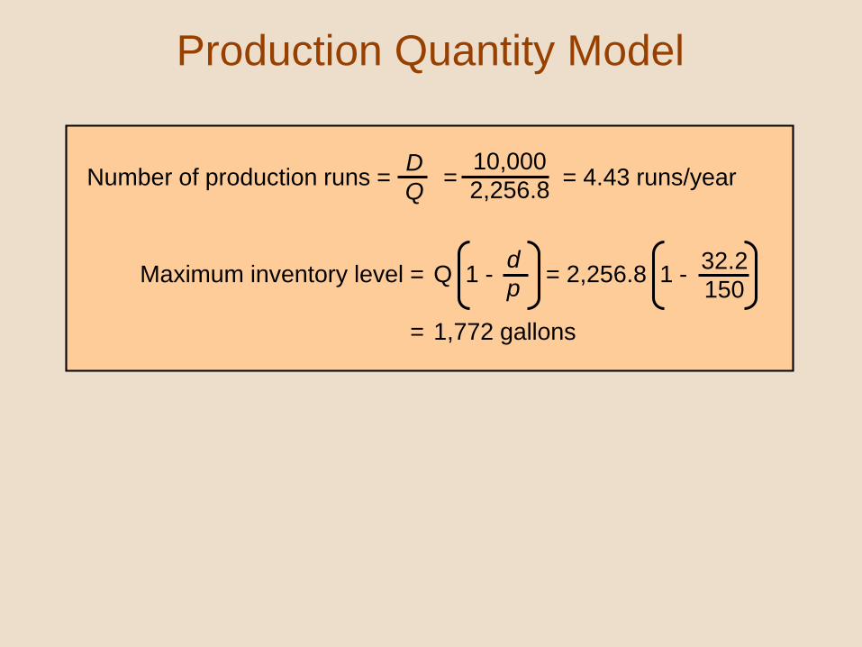
Production Quantity Model

Number of production runs = = = 4.43 runs/yearD

Q

10,000

2,256.8

Maximum inventory level = Q 1 - = 2,256.8 1 -

= 1,772 gallons

d

p32.2

150

Solution of EOQ Models With Excel

The optimal order

size, Q, in cell D8

Solution of EOQ Models With Excel

The formula for Q

in cell D10

=(D4*D5/D10)+(D3*D10/2)*(1-(D7/D8))

=D10*(1-(D7/D8))

Solution of EOQ Models With OM Tools

Quantity Discounts

Price per unit decreases as order

quantity increases

TC = + + PDCoD

Q

CcQ

2

where

P = per unit price of the item

D = annual demand

Quantity Discount Model

Qopt

Carrying cost

Ordering cost

Invento

ry c

ost ($

)

Q(d1 ) = 100 Q(d2 ) = 200

TC (d2 = $6 )

TC (d1 = $8 )

TC = ($10 )ORDER SIZE PRICE

0 - 99 $10

100 – 199 8 (d1)

200+ 6 (d2)

Quantity Discount

QUANTITY PRICE

1 - 49 $1,400

50 - 89 1,100

90+ 900

Co = $2,500

Cc = $190 per TV

D = 200 TVs per year

Qopt = = = 72.5 TVs2CoD

Cc

2(2500)(200)

190

TC = + + PD = $233,784 CoD

Qopt

CcQopt

2

For Q = 72.5

TC = + + PD = $194,105CoD

Q

CcQ

2

For Q = 90

Quantity Discount Model With Excel

=(D4*D5/E10)+(D3*E10/2)+C10*D5=IF(D10>B10,D10,B10)

Reorder Point

• Inventory level at which a new order is placed

R = dL

where

d = demand rate per period

L = lead time

Reorder Point

Demand = 10,000 gallons/year

Store open 311 days/year

Daily demand = 10,000 / 311 = 32.154

gallons/day

Lead time = L = 10 days

R = dL = (32.154)(10) = 321.54 gallons

Safety Stock

• Safety stock

• buffer added to on hand inventory during lead time

• Stockout

• an inventory shortage

• Service level

• probability that the inventory available during lead

time will meet demand

• P(Demand during lead time <= Reorder Point)

Variable Demand With Reorder Point

Reorder

point, R

Q

LT

Time

LT

Inve

nto

ry le

ve

l

0

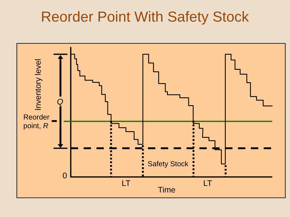
Reorder Point With Safety Stock

Reorder

point, R

Q

LTTime

LT

Inve

nto

ry le

ve

l

0

Safety Stock

Reorder Point With Variable Demand

R = dL + zd L

where

d = average daily demand

L = lead time

d = the standard deviation of daily demand

z = number of standard deviations

corresponding to the service level

probability

zd L = safety stock

Reorder Point For a Service Level

Probability of meeting demand during lead time = service level

Probability of a stockout

R

Safety stock

dL

Demand

zd L

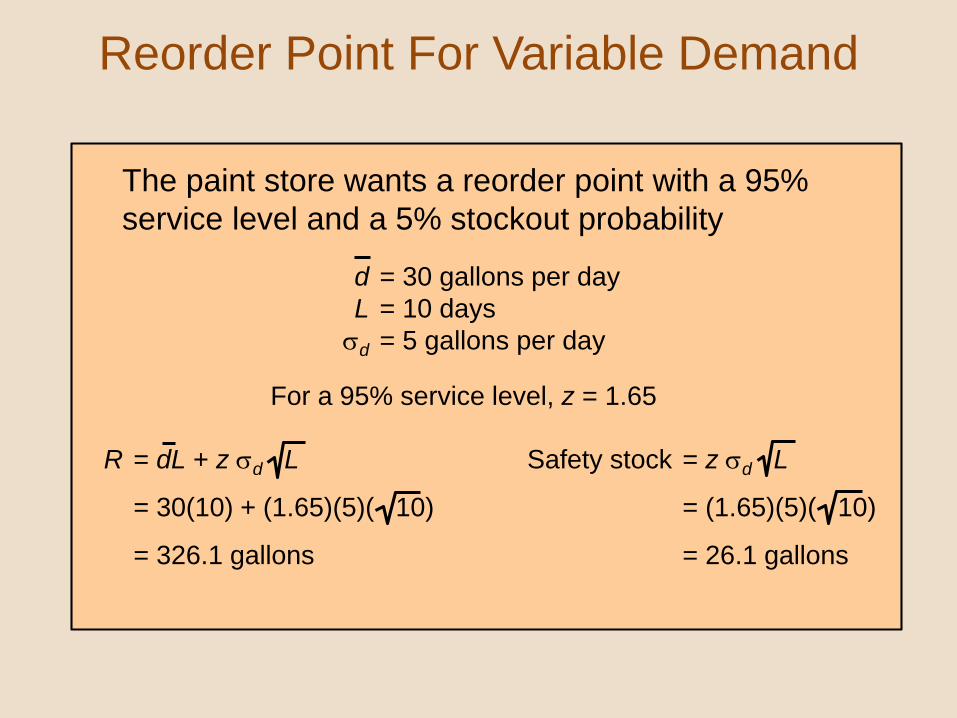
Reorder Point For Variable Demand

The paint store wants a reorder point with a 95%

service level and a 5% stockout probability

d = 30 gallons per day

L = 10 days

d = 5 gallons per day

For a 95% service level, z = 1.65

R = dL + z d L

= 30(10) + (1.65)(5)( 10)

= 326.1 gallons

Safety stock = z d L

= (1.65)(5)( 10)

= 26.1 gallons

Determining Reorder Point with Excel

The reorder point

formula in cell E7

Order Quantity for a Periodic Inventory System

Q = d(tb + L) + zd tb + L - I

where

d = average demand rate

tb = the fixed time between orders

L = lead time

d = standard deviation of demand

zd tb + L = safety stock

I = inventory level

Periodic Inventory System

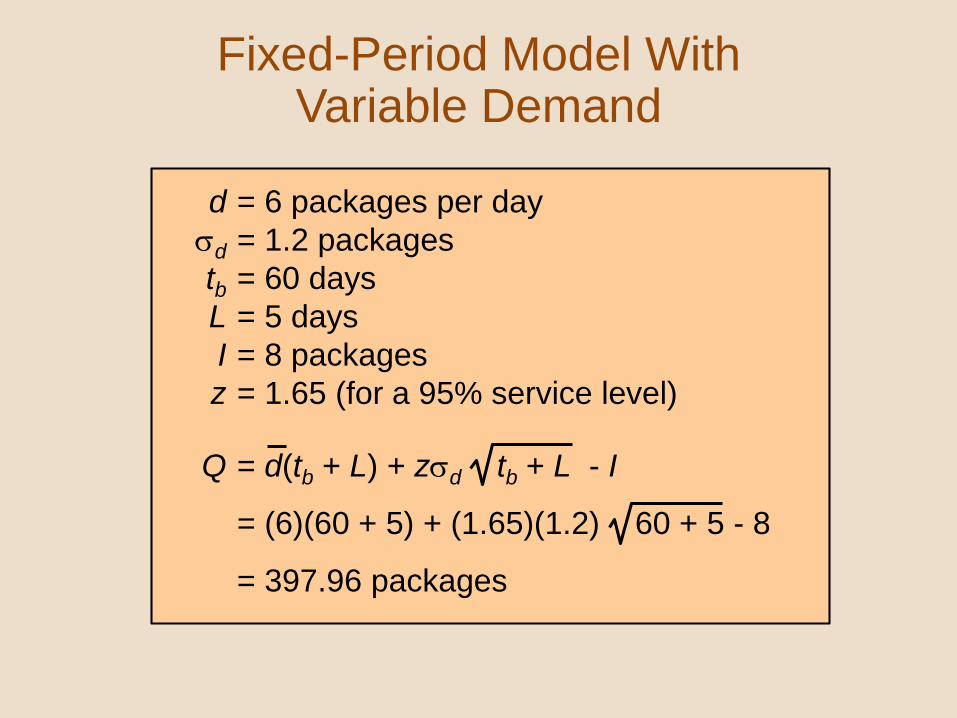
Fixed-Period Model With Variable Demand

d = 6 packages per day

d = 1.2 packages

tb = 60 days

L = 5 days

I = 8 packages

z = 1.65 (for a 95% service level)

Q = d(tb + L) + zd tb + L - I

= (6)(60 + 5) + (1.65)(1.2) 60 + 5 - 8

= 397.96 packages

Fixed-Period Model with Excel

Formula for order

size, Q, in cell D10