Knowledge discovery in a direct marketing case using least squares support vector machines

Knowledge Discovery in a DirectMarketing Case using Least SquaresSupport Vector MachinesS. Viaene,1, * B. Baesens,1 T. Van Gestel,2 J. A. K. Suykens,2

D. Van den Poel,3 J. Vanthienen,1 B. De Moor,2 G. Dedene1

1 K.U. Leuven, Department of Applied Economic Sciences, Naamsestraat 69,B-3000 Leuven, Belgium2 K.U. Leuven, Department of Electrical Engineering ESAT-SISTA, KasteelparkArenberg 10, B-3001 Leuven, Belgium3 Ghent University, Department of Marketing, Hoveniersberg 24, B-9000 Ghent,Belgium

We study the problem of repeat-purchase modeling in a direct marketing setting usingBelgian data. More specifically, we investigate the detection and qualification of the mostrelevant explanatory variables for predicting purchase incidence. The analysis is based ona wrapped form of input selection using a sensitivity based pruning heuristic to guide agreedy, stepwise, and backward traversal of the input space. For this purpose, we make

Ž .use of a powerful and promising least squares support vector machine LS-SVMclassifier formulation. This study extends beyond the standard recency frequency mone-

Ž . Ž .tary RFM modeling semantics in two ways: 1 by including alternative operationaliza-Ž . Ž .tions of the RFM variables, and 2 by adding several other non-RFM predictors.

Results indicate that elimination of redundant�irrelevant inputs allows significant reduc-tion of model complexity. The empirical findings also highlight the importance offrequency and monetary variables, while the recency variable category seems to be ofsomewhat lesser importance to the case at hand. Results also point to the added value ofincluding non-RFM variables for improving customer profiling. More specifically, cus-tomer�company interaction, measured using indicators of information requests andcomplaints, and merchandise returns provide additional predictive power to purchaseincidence modeling for database marketing. � 2001 John Wiley & Sons, Inc.

* Author to whom correspondence should be addressed; e-mail: [email protected].

ŽContract grant sponsor: Flemish government Research Council K.U. Leuven:.GOA-Mefisto; FWO-Flanders: ICCoS and AN-MMM; IWT: STWW Eureka .

Contract grant sponsor: Belgium government.Contract grant number: IUAP-IV�02, IV-24.Contract grant sponsor: European Commission.Contract grant number: TMR, ERNSI.

Ž .INTERNATIONAL JOURNAL OF INTELLIGENT SYSTEMS, VOL. 16, 1023�1036 2001� 2001 John Wiley & Sons, Inc.

VIAENE ET AL.1024

I. INTRODUCTION

The main objective of this paper involves the detection and qualification ofthe most relevant variables for repeat-purchase modeling in a direct marketingsetting. This knowledge is believed to vastly enrich customer profiling and thuscontribute directly to more targeted customer contact.

The empirical study focuses on the purchase incidence, i.e., the issuewhether or not a purchase is made from any product category offered by thedirect mailing company. Standard recency frequency monetary modeling seman-

1 Žtics underlie the discussed purchase incidence model. This binary buyer versus.nonbuyer classification problem is being tackled in this paper by using least

Ž .squares support vector machine LS-SVM classifiers. LS-SVMs have recentlybeen introduced in the literature2 and excellent benchmark results have beenreported.3 Having constructed an LS-SVM classifier with all available predictors,we engage in an input selection experiment. Input selection has been an activearea of research in the datamining field for many years now. A compact, yet

Ž .highly accurate model may come in very handy in on-line customer profilingsystems. Furthermore, by reducing the number of input features, both humanunderstanding and computational performance can often be vastly enhanced.

Section II elaborates on some response modeling issues including a litera-ture review and description of the data set. In Section III, we discuss the basicunderpinnings of LS-SVMs for binary classification. The input selection experi-ment and corresponding results are presented and discussed in Section IV.

II. THE RESPONSE MODELING CASE FOR DIRECT MARKETING

A. Response Modeling in Direct Marketing

Cullinan is generally credited for identifying the three sets of variables mostŽ . 1,4,5often used in response modeling: recency, frequency, and monetary RFM .

Since then, the literature has provided so many uses of these three variablecategories, that there is overwhelming evidence both from academically re-viewed studies as well as from practitioners’ experience that the RFM variablesare an important set of predictors for modeling mail-order repeat purchasing.However, the beneficial effect of including other variables into the responsemodel has also been investigated.

For mail-order response modeling, several alternative problem formulationshave been proposed based on the choice of the dependent variable. The firstcategory is purchase incidence modeling.6 In this problem formulation, the mainquestion is whether a customer will purchase during the next mailing period, i.e.,

Žone tries to predict the purchase incidence within a fixed time interval typically.half a year . Other authors have investigated related problems dealing with both

the purchase incidence and the amount of purchase in a joint model.7,8 A thirdalternative perspective for response modeling is to model interpurchase time

Ž .through survival analysis or split- hazard rate models which model whether apurchase takes place together with the duration of time until a purchase

KNOWLEDGE DISCOVERY IN DIRECT MARKETING 1025

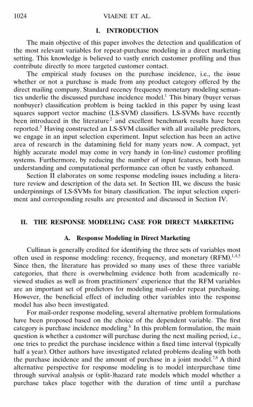
occurs.9,10 Table I provides a summary of contributions with regard to the threeŽ .alternative problem formulations. We observe that the first purchase incidence

formulation is clearly the most popular in the existing literature.11 Moreover,most studies include many predictors, even though only a minority includes allcategories.

This paper focuses on the first type of problem, i.e., purchase incidencemodeling. This choice is motivated by the fact that the majority of previousresearch in the direct marketing literature focuses on the purchase incidenceproblem.12,13 Furthermore, this is exactly the setting that mail-order companiesare typically confronted with. They have to decide whether or not a specific

Ž .offering will be sent to a potential customer during a certain mailing period.Given a tendency of rising mailing costs and increasing competition, we caneasily see an increasing importance for response modeling.14 Improving thetargeting of the offers may indeed counter these two challenges by lowering

Žnonresponse. Moreover, from the perspective of the recipient of the direct.mail messages, mail-order companies do not want to overload consumers with

catalogs. The importance of response modeling to the mail-order industry isfurther illustrated by the fact that the issue of improving targeting was amongthe top three concerns with 73.5% of the catalogers in the sample mentioned inRef. 15.

B. The Data Set

From a major Belgian mail-order company, we obtained data on pastpurchase behavior at the order-line level, i.e., we know when a customerpurchased what quantity of a particular product at which price as part of whatorder. This allowed us, in close cooperation with domain experts and guided bythe extensive literature, to derive all the necessary purchase behavior variablesfor a total sample size of 5,000 customers, of which 37.94% represent buyers.For each customer, these variables were measured for the period between 1 July1993 and 30 June 1997. The goal is to predict whether an existing customer willrepurchase in the observation period between 1 July 1997 and 31 December1997 using the information provided by the purchase behavior variables. Thisproblem boils down to a binary classification problem: Will a customer repur-chase or not? Notice that the focus is on customer retention and not oncustomer acquisition.

The recency, frequency, and monetary variables have then been modeled asdescribed in detail in Ref. 11. We used two time horizons for all RFM variables.The Hist horizon refers to the fact that the variable is measured for the periodbetween 1 July 1993 and 30 June 1997. The Year horizon refers to the fact thatthe variable is measured over the last year. Including both time horizons allowsus to check whether more recent data are more relevant than historical data. AllRFM variables are modeled both with and without the occurrence of returnedmerchandise, indicated by R and N in the variable name, respectively. Theformer is operationalized by including the counts of returned merchandise inthe variable values, whereas in the latter case these counts are omitted. Taking

VIAENE ET AL.1026

Tab

leI.

Lite

ratu

rere

view

ofre

spon

sem

odel

ing

pape

rs.

Inde

pend

entV

aria

ble

Dep

ende

ntV

aria

ble

Con

text

ofA

pplic

atio

n

Oth

erSo

cio-

Cat

alog

orB

ehav

iora

lD

emog

raph

icB

inar

y&

Bin

ary

&F

und-

Cat

alog

Spec

ialty

Ž.

Ref

eren

ceR

FM

Var

iabl

esV

aria

bles

Bin

ary

Am

ount

Tim

ing

Rai

sing

gene

ral

Mai

ling

16Ž

.B

erge

ran

dM

aglio

zzi

1992

XX

XX

XX

17Ž

.B

itran

and

Mon

dsch

ein

1996

XX

XX

X18

Ž.

Bul

tan

dW

ittin

k19

96X

XX

XX

19Ž

.B

ult

1993

XX

XX

X20

Ž.

Bul

tet

al.

1997

XX

XX

XX

X21

Ž.

Gon

ulan

dSh

i19

98X

XX

X¨

¨22

Ž.

Kas

low

1997

XX

XX

XX

X7

Ž.

Lev

inan

dZ

ahav

i19

98X

XX

XX

XX

X23

Ž.

Mag

liozz

iand

Ber

ger

1993

XX

XX

X24

Ž.

Mag

liozz

i19

89X

XX

XX

25Ž

.T

hras

her

1991

XX

XX

XX

10Ž

.V

ande

nPo

el&

Leu

nis

1998

XX

XX

XX

11Ž

.V

ande

nPo

el19

99X

XX

XX

XX

8Ž

.V

ande

rSc

heer

1998

XX

XX

Ž.1

3Z

ahav

iand

Lev

in19

97X

XX

XX

X


Ž .into account both time horizons Year versus Hist and inclusion versus exclu-Ž .sion of returned items R versus N , we arrive at a 2 � 2 design in which each

RFM variable is operationalized in four ways.For the recency variable, many operationalizations have already been

suggested. In this paper, we define the recency variable as the number of daysŽ .since the last purchase within a specific time window Hist versus Year and in-

Ž . 4or excluding returned merchandise R versus N . Recency has been found to beinversely related to the probability of the next purchase, i.e., the longer the timedelay since the last purchase the lower the probability of a next purchase withinthe specific period.1

In the context of direct mail, it has generally been observed that multibuy-Ž .ers buyers who already purchased several times are more likely to repurchase

than buyers who only purchased once.4,26 Although no detailed results arereported because of the proprietary nature of most studies, the frequencyvariable is generally considered to be the most important of the RFM variables� �12 . Bauer suggests to operationalize the frequency variable as the number ofpurchases divided by the time on the customer list since the first purchase.4 Wechoose to operationalize the frequency variable as the number of purchases

Ž .made in a certain time period Hist versus Year while in- or excluding returnedŽ .merchandise R versus N .

In the direct marketing literature, the general convention is that the moremoney a person has spent with a company, the higher his�her likelihood ofpurchasing the next offering.27 Nash suggests to operationalize monetary valueas the highest transaction sale or as the average order size.12 Levin and Zahavipropose to use the average amount of money per purchase.27 We model themonetary variable as the total accumulated monetary amount of spending by a

Ž .customer during a certain time period Hist versus Year while in- or excludingŽ .returned merchandise R versus N . Additionally, we include the natural loga-Ž .rithmic transformation ln of all monetary variables as a means to reduce the

skewness of the distributions.Apart from the RFM variables, we also included nine other customer

profiling inputs.11 The type and frequency of contact which customers have withthe mail-order company may yield important information about their futurepurchasing behavior. The GenInfo and GenCust are binary customer�companyinteraction variables indicating whether the customer asked for general informa-

Ž . Ž .tion respectively, filed general complaints . Since customer dis satisfaction maynot only be revealed by general complaints but also by returning items, weincluded two extra variables. The RetMerch variable is a binary variableindicating whether the customer has ever returned an item that was previouslyordered from the mail-order company. The RetPerc variable measures the totalmonetary amount of returned orders divided by the total amount of spending.The Ndays variable models the length of the customer relationship in days. It iscommonly believed that consumers�households with a longer relationship withthe company have a higher probability of repurchase than households withshorter relationships. IncrHist and IncrYear are operationalizations of a behav-ioral loyalty measure. We propose to perform a median split of the length of the

VIAENE ET AL.1028

Ž .relationship time since the household became a customer . This enables us toŽ .compare the number of purchases i.e., frequency between the first and last half

of the time window. The following formula is used:

purchases second half�purchases first half1Ž .

purchases first half

When the above measure is positive, this may give us an indication of increasingŽ .loyalty by that customer to the mail-order company, and ipso facto satisfaction

with the current level of service. Remember that the suffix Hist reflects that thewhole purchase history is used, whereas in the case of the suffix Year, onlytransactions from the last year are included. The ProdclaT respectively Prod-

Ž . � Ž .�claM variables represent the total T respectively, mean M forward-lookingweighted product index. The weighting procedure represents the ‘‘forward-look-ing’’ nature of a product category purchase, derived from another sample ofdata.

Table II gives an overview of the variables discussed above. Notice that allmissing values were handled by the mean imputation procedure28 and that allpredictor variables were normalized to zero mean and unit variance prior totheir inclusion in the model.29

III. LEAST SQUARES SVM CLASSIFICATION

A. LS-SVMs for Binary Classification

� 4N nGiven a training set x , y with input data x � � and correspondingi i i�1 i� 4binary class labels y � �1, �1 , the SVM classifier, according to Vapnik’si

original formulation,30 � 33 satisfies the following conditions:

wT� x � b � �1 if y � �1Ž .i i2Ž .

wT� x � b �1 if y � �1Ž .i i

Ž .Table II. A listing of all inputs both RFM and non-RFM includedin the direct marketing case.

Recency Frequency Monetary Other

RecYearR FrYearR MonHistR ProdclaTRecYearN FrYearN MonHistN ProdclaMRecHistR FrHistR MonYearR GenCustRecHistN FrHistN MonYearN GenInfo

Ž .ln MonHistR NdaysŽ .ln MonHistN IncrHistŽ .ln MonYearR IncrYearŽ .ln MonYearN RetMerch

RetPerc


which is equivalent to:

Ty w � x � b � 1 i � 1, . . . , N 3Ž . Ž .i i

Ž . n nhThe nonlinear function � � : � � � maps the input space to a high dimen-Ž .sional and possibly infinite dimensional feature space. In primal weight space

the classifier then takes the form:

Ty x � sign w � x � b 4Ž . Ž . Ž .

however, it is never evaluated in this form. One defines the optimizationproblem as:

N1Tmin TT w , � � w w � c � 5Ž . Ž .Ý i2w , b , � i�1

subject to:

Ty w � x � b � 1 � � i � 1, . . . , NŽ .i i i6Ž .

� � 0 i � 1, . . . , Ni

The variables � are slack variables which are needed to allow misclassificationsiŽ .in the set of inequalities e.g., due to overlapping distributions . The positive real

constant c should be considered as a tuning parameter in the algorithm. Fornonlinear SVMs, the QP-problem and the classifier are never solved andevaluated in this form. Instead, a dual space formulation and representation are

Ž .obtained by applying the Mercer condition see Refs. 30�33 for details .Vapnik’s SVM classifier formulation was modified by Suykens and Vande-

walle2 into the following LS-SVM formulation:

N1 1T 2min TT w , e � w w � � e 7Ž . Ž .Ý i2 2w , b , e i�1

subject to the equality constraints:

Ty w � x � b � 1 � e , i � 1, . . . , N 8Ž . Ž .i i i

This formulation now consists of equality instead of inequality constraints andtakes into account a squared error with a regularization term similar to ridgeregression. The solution is obtained after constructing the Lagrangian:

NTLL w , b , e ; � � TT w , e � � y w � x � b � 1 � e 9Ž . Ž . Ž . Ž .� 4Ý i i i i

i�1

where � are the Lagrange multipliers. After taking the conditions for optimal-iity, one obtains the following linear system2:

T b 00 Y� 10Ž .�1 � 1Y � � � I

VIAENE ET AL.1030

� Ž .T Ž .T � � � � �where Z � � x y ; . . . ; � x y , Y � y ; . . . ; y , 1 � 1; . . . ; 1 , � �1 1 N N 1 N� � T 2� ; . . . ; � , � � ZZ , and Mercer’s condition is applied within the � matrix:1 N

T� � y y � x � xŽ . Ž .i j i j i j

11Ž .� y y K x , xŽ .i j i j

Ž .For the kernel function K �, � one typically has the following choices:

K x , x � xT x , linear kernelŽ . Ž .i i

dTK x , x � x x � 1 , polynomial kernel of degree dŽ . Ž .Ž .i i

� � 2 2K x , x � exp � x � x �� , radial basis function RFB kernelŽ . Ž .Ž .� 42i i

K x , x � tanh xT x � , multilayer perceptron MLP kernelŽ . Ž .Ž .Ž .i i

where d, � , , and are constants. Notice that the Mercer condition holds forall � � �� and d � � values in the RBF and the polynomial cases, but not forall possible choices of and in the MLP case. The LS-SVM classifier is thenconstructed as follows:

N

y x � sign � y K x , x � b 12Ž . Ž . Ž .Ý i i ii�1

Ž . Ž . Ž .Note that the matrix in 10 is of dimension N � 1 � N � 1 . For large valuesof N, this matrix cannot easily be stored, such that an iterative solution methodfor solving it is needed. A Hestenes�Stiefel conjugate gradient algorithm issuggested in Ref. 34 to overcome this problem. Basically, the latter rests upon a

Ž . 34transformation of the matrix in 10 to a positive definite form. A straightfor-ward extension of LS-SVMs to multiclass problems has been proposed in Ref.35, where additional outputs are taken to encode multiclasses as is often done inclassical neural network methodology.29 A drawback of LS-SVMs is that sparse-ness is lost due to the choice of a 2-norm. However, this can be circumvented ina second stage by a pruning procedure which is based upon removing trainingpoints guided by the sorted support value spectrum.36

B. Calibrating the RBF LS-SVM Classifier

All classifiers were trained using RBF kernels.3 Estimation of the general-ization ability of the RBF LS-SVM classifier is then realized by the followingexperimental setup3:

3 1Ž .1 Set aside of the data for the training set and the remaining for testing,4 4respecting the original class distribution.

Ž . Ž .2 Perform 10-fold cross validation on the training data for each � , � combina-tion from the initial candidate tuning sets � and � typically chosen as follows:

'� 4� � 0.5, 5, 10, 15, 25, 50, 100, 250, 500 � n

1� 4� � 0.01, 0.5, 1, 10, 50, 100, 500, 1000 �

N


2' � �The square root n of the number of inputs n is introduced, since x � x in2i1the RBF kernel is proportional to n and the factor is introduced such that theN

misclassification term �ÝN e2 is normalized with the size of the data set.i�1 iŽ . Ž .3 Choose optimal � , � from the initial candidate tuning sets � and � by looking

Ž .at the best cross validation performance for each � , � combination.Ž .4 Refine � and � iteratively by means of a grid search mechanism to further

Ž .optimize the tuning parameters � , � . In our experiments, we repeated thisstep three times.

Ž .5 Construct the LS-SVM classifier using the total training set for the optimalŽ .choice of the tuned hyperparameters � , � .

Ž .6 Assess the generalization ability by means of the independent test set.

Following the procedure outlined above, one obtained the results depicted3in Table III. The optimized RBF LS-SVM classifier, trained on of the data set,4

achieves a percentage correctly classified on the training data of 77.54% with� � 13.75 and � � 1.50. Performance on the independent test data amounts to74.48% correctly classified. We contrasted these results with those obtainedusing a linear kernel for the LS-SVM classifier. As can be observed from TableIII, the percentage correctly classified drops to 76.26% on the training set and to73.76% on the independent test set.

IV. THE INPUT SELECTION EXPERIMENT

A. Input Selection in a Nutshell

Input selection is a commonly adhered technique to reduce model complex-ity. The goal is to find a reduced coordinate system that allows one to projectthe data on a more compact representation. The general assumption underlyingthis operation and justifying it, is that the studied data approximately lie withinthe bounds of this reduced space. As such, models with fewer inputs are capableof improving both human understanding and computational performance. More-over, elimination of redundant and�or irrelevant inputs may also improve thepredictive power of an algorithm.37 Selecting the best subset of a set of npredictors is a nontrivial problem. This follows from the fact that the optimalinput subset can only be obtained when the input space is exhaustively searched.When n inputs are present, this would imply the need to evaluate 2 n�1 inputsubsets. Unfortunately, as n grows, this very quickly becomes computationallyinfeasible. For that reason, heuristic search procedures are often preferred.Input selection can then either be performed as a preprocessing step, indepen-

Table III. Classification accuracy of the optimized RFB LS-SVMclassifier versus an LS-SVM optimized using a linear kernel.

LS-SVM LS-SVMClassification Accuracy RBF Kernel Linear Kernel

Ž .Training 3750 observations 77.54% 76.26%Ž .Test 1250 observations 74.48% 73.76%

VIAENE ET AL.1032

dent of the induction algorithm, or explicitly make use of it. The formerapproach is termed filter, the latter wrapper.38 Filter methods operate indepen-dently of the learning algorithm. Undesirable inputs are filtered out of the databefore induction commences. Focus39 and Relief 40 are well-known filter meth-ods. Wrapper methods make use of the actual target learning algorithm toevaluate the usefulness of inputs. Typically, the input evaluation heuristic that isused is based upon inspection of the trained parameters and�or comparison ofpredictive performance under different input subset configurations. Input selec-tion is then often performed in a sequential fashion, e.g., guided by a best-firstinput selection strategy. The backward selection scheme starts from a full inputset and stepwise prunes input variables that are undesirable. The forwardselection scheme starts from the empty input set and stepwise adds inputvariables that are desirable. Hybrids of the above also exist.

B. Wrapping the Optimized LS-SVM Classifier

Input selection effectively starts at the moment the LS-SVM classifier hasbeen constructed on the full set of n available predictors. The input selection

Ž .procedure is based upon a greedy best-first heuristic, guiding a backwardsearch mechanism through the input space.38 The mechanics of the imple-mented heuristic for assessing the sensitivity of the classifier to a certain inputare quite straightforward. We apply a strategy of constant substitution in whichan input is perturbed to its mean while all other inputs keep their values andcompute the impact of this operation on the performance of the obtainedLS-SVM classifier without reestimation of the LS-SVM parameters � and b.This assessment is done using the separate pruning set to obtain an unbiasedestimate of the change in classification accuracy of the constructed classifier.The pruning set consists of 1250 observations that were randomly selected fromthe training set of 3750 observations. Figure 1 provides a concise overview of thedifferent steps of the experimental procedure.

Figure 1.


Starting with a full input set F , all n inputs are pruned sequentially, i.e.,1one by one. The first input f to be removed, is determined at the end of Step 1p� Ž .�task 4 . After having removed this input from F , the reduced input set1

� 4F � F f is used for subsequent input removal. At this moment, an itera-2 1 ption of identical Steps i is started, in which, in a first phase, the LS-SVM

� Ž . �parameters � and b are re-estimated on the training set task 1 of Step i ,however, without recalibration for � and � , and the generalization ability of the

� Ž . �classifier is quantified on the independent test set task 2 of Step i . Notice thatŽ .the originally optimized � and � values obtained in task 1 of Step 1 remain

unchanged during the entire input selection phase. Again, input sensitivities ofŽ .the resulting classification model without re-estimation of � and b are

assessed on the pruning set to identify the input to which the classifier is least� Ž . �sensitive when perturbed to its mean task 3 of Step i . This input is then

pruned from the remaining input subset and disregarded for further analysis.The pruning procedure is thereupon resumed with a reduced input set, until allinputs are eventually removed. Once all inputs have been pruned, the preferredreduced model is then determined by means of the highest pruning set perfor-mance.

Table IV summarizes the empirical findings of the pruning procedure forthe RFM case. Observe how the suggested input selection method allows

Ž .significant reduction of model complexity from 25 to 9 inputs without anysignificant degradation of the generalization behavior on the independent testset. The test set performance amounts to 73.92% for the full model and 73.52%for the reduced model.

The order of input removal as depicted in Table V, provides further insightŽ .into the relative importance of the predictor categories cf. Table II . The

reduced model consists of the nine inputs that are underlined in Table V. ThisŽ .reduced set of predictors consists of frequency, monetary, and other non-RFM

variables. It is especially important to note that the reduced model includesinformation on returned merchandise. Furthermore, notice the absence of therecency component in the reduced input set. Inspection of the order of removalof inputs, while further pruning this reduced input set, highlights the relativeimportance of the frequency variables. More specifically, the last two variablesto be removed belong to this predictor category. Note that an input setconsisting of only these two inputs, still yields a percentage correctly classified at72.00% on the test set. Results also point to the beneficial effect of including the

Table IV. Empirical assessment of the RBF LS-SVM classifiers forthe full and reduced models.

Classification Accuracy Full Model Reduced Model

Ž .Training 2500 observations 77.36% 76.04%Ž .Pruning 1250 observations 76.72% 77.20%

Ž .Test 1250 observations 73.92% 73.52%Number of Inputs 25 9

VIAENE ET AL.1034

Table V. Order of input removal. Each input is qualified by its category with r, f, m andŽ .o respectively standing for recency, frequency, monetary and other cf. Table II .

Pruning Steps

1�5 6�10 11�15 16�20 21�25

RetPerc o ProdclaM o RecHistN r FrYearN f MonYearR mŽ . Ž .ln MonHistN m MonHistR m IncrHist o ln MonHistR m MonYearN m

RecHistR r IncrYear o RecYearR r MonHistN m GenInfo oŽ .Ndays o ln MonYearR m RecYearN r GenCust o FrHistR fŽ .ProdclaT o ln MonYearN m FrHistN f RetMerch o FrYearR f

non-RFM customer profiling variables GenInfo and GenCust for improvingpredictive accuracy. They underline that customer�company interaction vari-ables, here measured by indicators of information requests and complaints,provide additional predictive power to purchase incidence modeling for databasemarketing.

V. CONCLUSION

In this paper, we applied an LS-SVM based input selection wrapper to areal-life direct marketing case involving the modeling of repeat-purchase behav-ior. Based on a thorough review of the literature, we extended the well-known

Ž . Ž .recency, frequency, monetary RFM framework 1 by using alternative opera-Ž .tionalizations of the original variables, and 2 by including several additional

behavioral variables. The sensitivity based, stepwise input selection method,constructed as a wrapper around the LS-SVM classifier, allows significantreduction of model complexity without degrading predictive performance. Theempirical findings highlight the role of frequency and monetary variables in thereduced model, while the recency variable category seems to be of somewhatlesser importance within the response model. Results also point to the beneficialeffect of including non-RFM customer profiling variables for improving predic-tive accuracy. More specifically, customer�company interaction, measured byindicators of information requests and complaints, and merchandise returnsprovide additional predictive power to purchase incidence modeling for databasemarketing.

This work was partly carried out at the Leuven Institute for Research on Informa-Ž .tion Systems LIRIS of the Department of Applied Economic Sciences of the K.U.

Leuven in the framework of the KBC Insurance Research Chair. This work was partlycarried out at the ESAT laboratory and the Interdisciplinary Center of Neural NetworksICNN of the K.U. Leuven. S. Viaene, holder of the KBC Insurance Research Chair, andB. Baesens are both Research Assistants of LIRIS. T. Van Gestel is a research assistant

Ž .with the Fund for Scientific Research Flanders FWO-Flanders , J. Suykens is a postdoc-Ž .toral researcher with the Fund for Scientific Research Flanders FWO-Flanders , B. De

Moor is a senior research associate with the Fund for Scientific Research FlandersŽ .FWO-Flanders . D. Van den Poel is an assistant professor at the Department of


Marketing at Ghent University. J. Vanthienen and G. Dedene are Senior ResearchAssociates of LIRIS.

References

1. Cullinan GJ. Picking them by their batting averages’ recency-frequency-monetarymethod of controlling circulation. Direct Mail�Marketing Association, New York,manual release 2103 edition, 1977.

2. Suykens JAK, Vandewalle J. Least squares support vector machine classifiers. NeuralŽ .Process Lett 1999;9 3 :293�300.

3. Van Gestel T, Suykens JAK, Baesens B, Viaene S, Vanthienen J, Dedene G, DeMoor B, Vandewalle J. Benchmarking least squares support vector machine classi-fiers. Technical Report 00-37, ESAT-SISTA, K.U. Leuven, Leuven, Belgium, 2000.

Ž .4. Bauer A. A direct mail customer purchase model. J Direct Marketing 1988;2 3 :16�24.5. Kestnbaum RD. Quantitative database methods. In: The direct marketing handbook.

New York: McGraw Hill; 1992. p 588�597.6. Bult JR. Target selection for direct marketing, PhD thesis, Groningen University,

1993.7. Levin N, Zahavi J. Continuous predictive modeling: a comparative analysis. J Interac-

Ž .tive Marketing 1998;12 2 :5�22.8. Van der Scheer HR. Quantitative approaches for profit maximization in direct

marketing, PhD thesis, Groningen University, 1998.9. Dekimpe MG, Degraeve Z. The attrition of volunteers. European J Operat Res

1997;98:37�51.10. Van den Poel D, Leunis J. Database marketing modeling for financial services using

hazard rate models. Internat Rev Retail, Distribution and Consumer Res 1998;Ž .8 2 :243�257.

11. Van den Poel D. Response Modeling for Database Marketing using Binary Classifi-cation, PhD thesis, K.U. Leuven, 1999.

12. Nash EL. Direct marketing: strategy, planning, execution. Third Ed. New York:McGraw Hill; 1994.

13. Zahavi J, Levin N. Issues and problems in applying neural computing to targetŽ .marketing. J Direct Marketing 1997;11 4 :63�75.

14. Hauser B. List Segmentation. In: The direct marketing handbook. New York:McGraw-Hill; 1992. p 233�247.

15. DMA. Statistical fact book 1998. Twentieth Ed. New York: Direct MarketingAssociation; 1998.

16. Berger P, Magliozzi T. The effect of sample size and proportion of buyers in thesample on the performance of list segmentation equations generated by regression

Ž .analysis. J Direct Marketing 1992;6 1 :13�22.17. Bitran GR, Mondschein SV. Mailing decisions in the catalog sales industry. Manage

Ž .Sci 1996;42 9 :1364�1381.18. Bult JR, Wittink DR. Estimating and validating asymmetric heterogeneous loss

functions applied to health care fund raising. Int J Res Marketing 1996;13:215�226.19. Bult JR. Semiparametric versus parametric classification models: an application to

direct marketing. J Marketing Res 1993;30:380�390.20. Bult JR, Van der Scheer H, Wansbeek T. Interaction between target and mailing

characteristics in direct marketing, with an application to health care fund raising. IntJ Res Marketing 1997;14:301�308.

21. Gonul F, Shi MZ. Optimal mailing of catalogs: a new methodology using estimable¨ ¨Ž .structural dynamic programming models. Manage Sci 1998;44 9 :1249�1262.

22. Kaslow GA. A microeconomic analysis of consumer response to direct marketing andmail order, PhD thesis, California Institute of Technology, 1997.

VIAENE ET AL.1036

23. Magliozzi TL, Berger PD. List segmentation strategies in direct marketing. OmegaŽ .Int J Manage Sci 1993;21 1 :61�72.

24. Magliozzi TL. An empirical investigation of regression meta-strategies for directmarketing list segmentation models, PhD thesis, Boston University, 1989.

25. Thrasher RP. Cart: a recent advance in tree-structured list segmentation methodol-Ž .ogy. J Direct Marketing 1991;5 1 :35�47.

26. Stone B. Successful direct marketing methods. Chicago: Crain books; 1984.27. Levin N, Zahavi J. Segmentation analysis with managerial judgment. J Direct

Ž .Marketing 1996;10 3 :28�47.28. Little RJA. Regression with missing x’s: a review. J Amer Statist Assoc

Ž .1992;87 420 :1227�1230.29. Bishop CM. Neural networks for pattern recognition. New York: Oxford University

Press; 1995.30. Cristianini N, Shawe-Taylor J. An introduction to support vector machines. Cam-

bridge, UK: Cambridge University Press; 2000.31. Smola A. Learning with kernels, PhD thesis, Technical University, Berlin, 1999.32. Vapnik V. The nature of statistical learning theory. New York: Springer-Verlag;

1995.33. Vapnik V. Statistical learning theory. New York: John Wiley & Sons; 1998.34. Suykens JAK, Lukas L, Van Dooren P, De Moor B, Vandewalle J. Least squares

support vector machine classifiers: a large scale algorithm. In: 14th EuropeanConference on Circuits Theory and Design, Stresa, Italy, 1999. p 839�842.

35. Suykens JAK, Vandewalle J. Multiclass least squares support vector machines. In:10th International Joint Conference on Neural Networks, Washington DC, 1999.

36. Suykens JAK, Lukas L, Vandewalle J. Sparse least squares support vector machineclassifiers. In: 9th European Symposium on Artificial Neural Networks, Bruges,Belgium; 2000. p 37�42.

37. Bellman RE. Adaptive control processes. Princeton: Princeton University Press;1961.

38. John G, Kohavi R, Pfleger K. Irrelevant features and the subset selection problem.In: Machine Learning: Proc Eleventh Int Conf, San Francisco, California, 1994. p121�129.

39. Almuallim H, Dietterich TG. Learning with many irrelevant features. In: Ninth NatConf on Artificial Intelligence, Anaheim, California. Menlo Park, CA: AAAI Press;1991. p 547�552.

40. Kira K, Rendell LA. The feature selection problem: Traditional methods and a newalgorithm. In: Tenth Nat Conf on Artificial Intelligence, San Jose, California. MenloPark, CA: AAAI Press; 1992. p 129�134.

Documents

Knowledge discovery in a direct marketing case using least squares support vector machines