Embed Size (px)
DESCRIPTION
Kohring
Citation preview
Design and Construction of a Hydrostatic Dynamometer for Testing a Hydraulic Hybrid Vehicle
A THESIS SUBMITTED TO THE FACULTY OF THE GRADUATE SCHOOL
OF THE UNIVERSITY OF MINNESOTA BY
Henry Julian Kohring
IN PARTIAL FULFILLMENT OF THE REQUIREMENTS
FOR THE DEGREE OF MASTER OF SCIENCE
Perry Y. Li, Thomas R. Chase, Co-advisers
July, 2012

© Henry Julian Kohring 2012
i
Acknowledgements
I would like to thank my advisers, Professors Perry Li and Thomas Chase for their support and
advice on this project.
Without the help of my fellow students, this project would not have been possible. Although
many more students contributed to my work, some stand out as being particularly helpful. Kai
Loon Cheong provided invaluable advice in designing and troubleshooting the dynamometer.
Zhekang Du designed and implemented a controller necessary for the operation of the
dynamometer. Andrew Harm skillfully assembled parts of both the dynamometer and hydraulic
hybrid vehicle. Jonathan Meyer contributed his great knowledge of the vehicle. Professor
Zongxuan Sun's students, Ke Li and Michael Koester, shared their workspace.
Mechanical Engineering department staff greatly aided my work. Larissa Gonring, Holly Edgett,
and the rest of the University of Minnesota's Purchasing staff deserve my gratitude for their
patience, accuracy, and attention to detail in processing the 104 purchase orders necessary to
make this project a success. Stores Specialist Mark Erickson received those orders and often
helped me find hardware, even when I did not know specifically what I needed. Patrick Nelsen
and Robin Russell from the Mechanical Engineering Research Shop completed quality
manufacturing work for the vehicle in days that would have taken me weeks.
Funding by the US National Science Foundation through the Center for Compact and Efficient
Fluid Power under grant #EEC 0540834 is gratefully acknowledged.
ii
Abstract
A hydrostatic dynamometer has been constructed to test a hydraulic hybrid passenger vehicle.
Hybrid vehicles reduce their fuel consumption by capturing energy normally lost during braking
and reusing it during acceleration in addition to managing the engine to enable it to run at a
higher efficiency operating point. The dynamometer is designed to test a particular hybrid
vehicle which stores and transmits energy hydraulically. Measurement of fuel consumption
while the vehicle completes standard drive cycles is necessary to refine and validate the
performance and efficiency of the vehicle. The dynamometer provides repeatable, convenient,
inexpensive, safe, and flexible indoor testing for the vehicle.
The dynamometer connects directly to the output shaft of the vehicle's transmission. It is
mounted on a bedplate installed behind the vehicle. The dynamometer's hydraulic pump loads
or motors the vehicle to simulate driving. It can be controlled either manually or automatically.
Automatic controls allow the dynamometer to calculate and apply the appropriate load based
on vehicle speed.
MATLAB and Simulink simulations aided the design of the dynamometer. A MATLAB simulation
of the vehicle determined torque and speed requirements for standard drive cycles. Another
MATLAB simulation calculated pressures, flow rates, and energy storage requirements on the
dynamometer to size components. A Simulink simulation aided controls development.
The dynamometer has demonstrated open and closed loop performance with and without load.
It has demonstrated fast torque tracking. However, vehicle reliability issues have prevented
drive cycle tests from being completed.
iii
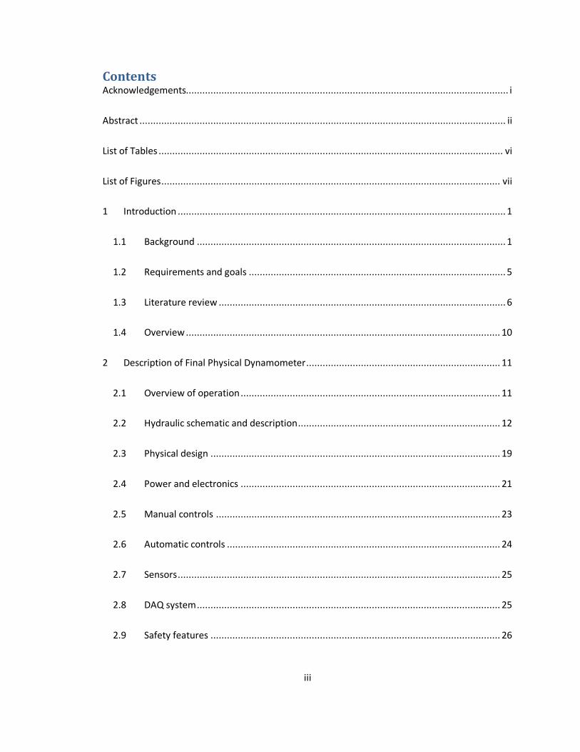
Contents Acknowledgements...................................................................................................................... i
Abstract ...................................................................................................................................... ii
List of Tables .............................................................................................................................. vi
List of Figures ............................................................................................................................ vii
1 Introduction ........................................................................................................................ 1
1.1 Background ................................................................................................................. 1
1.2 Requirements and goals .............................................................................................. 5
1.3 Literature review ......................................................................................................... 6
1.4 Overview ................................................................................................................... 10
2 Description of Final Physical Dynamometer ....................................................................... 11
2.1 Overview of operation ............................................................................................... 11
2.2 Hydraulic schematic and description .......................................................................... 12
2.3 Physical design .......................................................................................................... 19
2.4 Power and electronics ............................................................................................... 21
2.5 Manual controls ........................................................................................................ 23
2.6 Automatic controls .................................................................................................... 24
2.7 Sensors ...................................................................................................................... 25
2.8 DAQ system ............................................................................................................... 25
2.9 Safety features .......................................................................................................... 26
iv
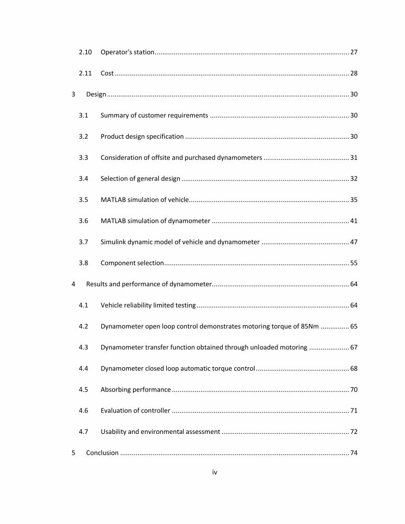
2.10 Operator's station ...................................................................................................... 27
2.11 Cost ........................................................................................................................... 28
3 Design ............................................................................................................................... 30
3.1 Summary of customer requirements ......................................................................... 30
3.2 Product design specification ...................................................................................... 30
3.3 Consideration of offsite and purchased dynamometers ............................................. 31
3.4 Selection of general design ........................................................................................ 32
3.5 MATLAB simulation of vehicle .................................................................................... 35
3.6 MATLAB simulation of dynamometer ........................................................................ 41
3.7 Simulink dynamic model of vehicle and dynamometer .............................................. 47
3.8 Component selection ................................................................................................. 55
4 Results and performance of dynamometer........................................................................ 64
4.1 Vehicle reliability limited testing ................................................................................ 64
4.2 Dynamometer open loop control demonstrates motoring torque of 85Nm ............... 65
4.3 Dynamometer transfer function obtained through unloaded motoring ..................... 67
4.4 Dynamometer closed loop automatic torque control ................................................. 68
4.5 Absorbing performance ............................................................................................. 70
4.6 Evaluation of controller ............................................................................................. 71
4.7 Usability and environmental assessment ................................................................... 72
5 Conclusion ........................................................................................................................ 74
v
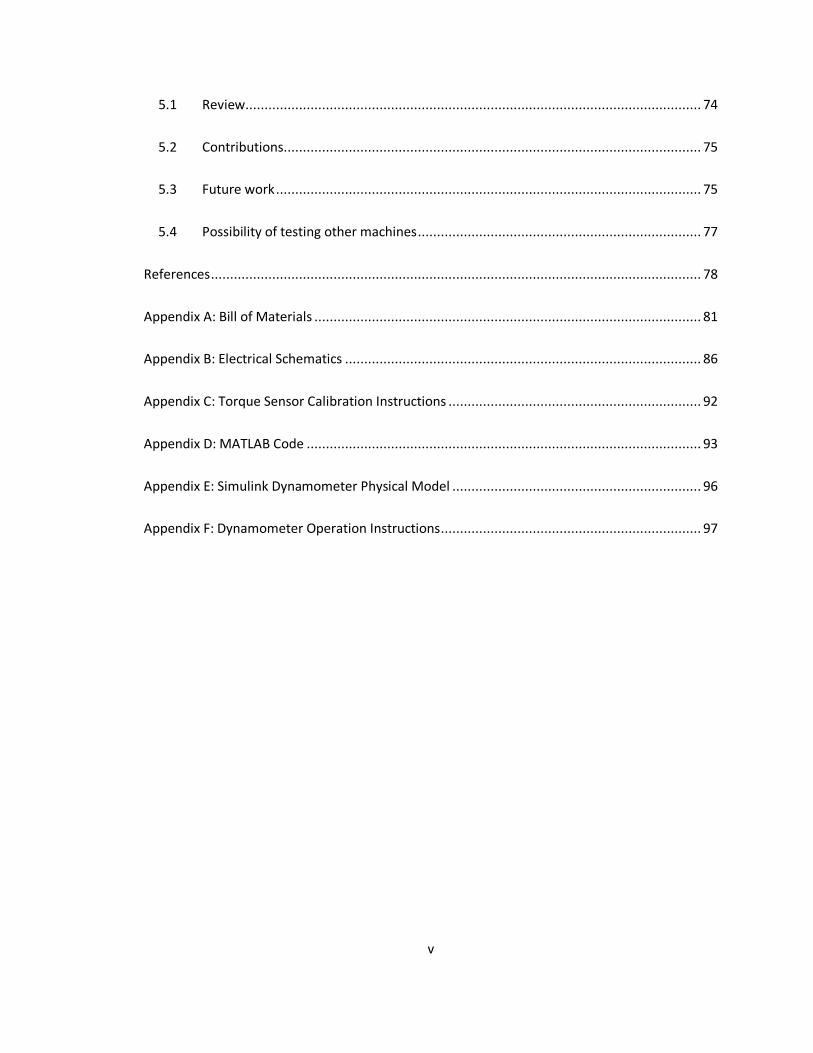
5.1 Review ....................................................................................................................... 74
5.2 Contributions............................................................................................................. 75
5.3 Future work ............................................................................................................... 75
5.4 Possibility of testing other machines .......................................................................... 77
References ................................................................................................................................ 78
Appendix A: Bill of Materials ..................................................................................................... 81
Appendix B: Electrical Schematics ............................................................................................. 86
Appendix C: Torque Sensor Calibration Instructions .................................................................. 92
Appendix D: MATLAB Code ....................................................................................................... 93
Appendix E: Simulink Dynamometer Physical Model ................................................................. 96
Appendix F: Dynamometer Operation Instructions.................................................................... 97
vi
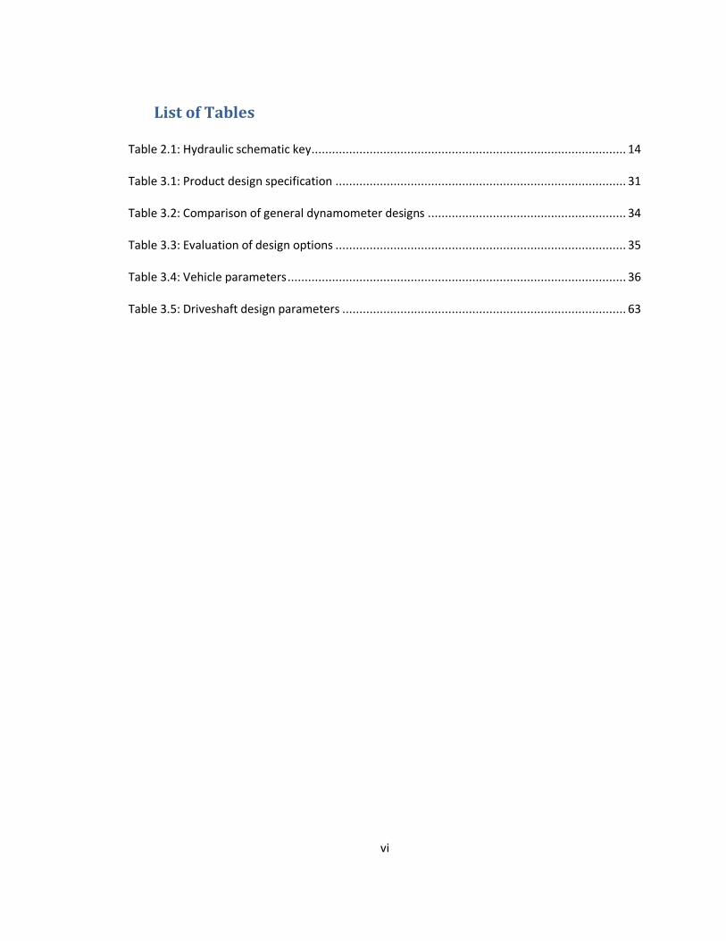
List of Tables
Table 2.1: Hydraulic schematic key............................................................................................ 14
Table 3.1: Product design specification ..................................................................................... 31
Table 3.2: Comparison of general dynamometer designs .......................................................... 34
Table 3.3: Evaluation of design options ..................................................................................... 35
Table 3.4: Vehicle parameters ................................................................................................... 36
Table 3.5: Driveshaft design parameters ................................................................................... 63
vii
List of Figures
Figure 1.1: The Generation 1 HHPV ............................................................................................. 1
Figure 1.2: Input coupled power split architecture ...................................................................... 4
Figure 1.3: EPA's Urban Dynamometer Driving Schedule[4] ......................................................... 6
Figure 1.4: EPA drive cycle speed tolerances[5] ........................................................................... 7
Figure 2.1: Block diagram of vehicle and dynamometer ............................................................ 11
Figure 2.2: Vehicle connected to dynamometer ........................................................................ 12
Figure 2.3: Dynamometer hydraulic schematic .......................................................................... 13
Figure 2.4: Overall physical dynamometer ................................................................................ 20
Figure 2.5: Block diagram of electrical system ........................................................................... 22
Figure 2.6: Manual control box ................................................................................................. 23
Figure 2.7: Operator's station .................................................................................................... 28
Figure 3.1: EPA UDDS speed ...................................................................................................... 37
Figure 3.2: EPA UDDS wheel speed............................................................................................ 38
Figure 3.3: EPA UDDS wheel torque .......................................................................................... 38
Figure 3.4: EPA HWFET speed ................................................................................................... 39
Figure 3.5: EPA HWFET wheel speed ......................................................................................... 39
Figure 3.6: EPA HWFET wheel torque ........................................................................................ 40
Figure 3.7: Volume of fluid in accumulator versus time drops below 0 in the vicinity of 300s and
750s corresponding to the HWFET ............................................................................................ 44
Figure 3.8: Pressure at dynamometer driving pump corresponding to the HWFET .................... 44
Figure 3.9: Manually varied dynamometer driving pump displacement during HWFET cycle ..... 46
viii
Figure 3.10: Volume of fluid in accumulator remains positive if dynamometer dynamometer
driving pump displacement is varied according to Figure 3.9 during the HWFET ........................ 46
Figure 3.11: Dynamometer driving pump pressure magnitude remains below 200bar even during
periods of reduced dynamometer driving pump displacement on HWFET ................................. 47
Figure 3.12: Overview of Simulink vehicle and dynamometer model ......................................... 48
Figure 3.13: Overview of dynamometer Simulink model ........................................................... 48
Figure 3.14: Physical dynamometer model block diagram ......................................................... 50
Figure 3.15: Simulated open loop performance of dynamometer motoring .............................. 53
Figure 3.16: Dynamometer controller block diagram ................................................................. 54
Figure 3.17: Imperfect simulated torque tracking using an example controller .......................... 55
Figure 3.18: Proportional valve verification circuit..................................................................... 58
Figure 3.19: Pump speed versus command voltage for proportional valve test.......................... 59
Figure 3.20: Pump torque magnitude versus command voltage for the proportional valve test . 59
Figure 4.1: Dynamometer open loop torque and speed............................................................. 66
Figure 4.2: Dynamometer system ID Bode plot ......................................................................... 67
Figure 4.3: Closed loop torque control ...................................................................................... 69
Figure 4.4: Dynamometer absorbing performance .................................................................... 71
1
1 Introduction
The purpose of this chapter is to introduce the project and explain the motivation for it. It
describes the dynamometer and the vehicle it is designed to test in section 1.1. It describes the
goals of the project in section 1.2. This chapter also summarizes some other hydrostatic and
non-hydrostatic dynamometers designed to test vehicles in section 1.3. An outline of the rest of
this thesis appears in section 1.4.
1.1 Background
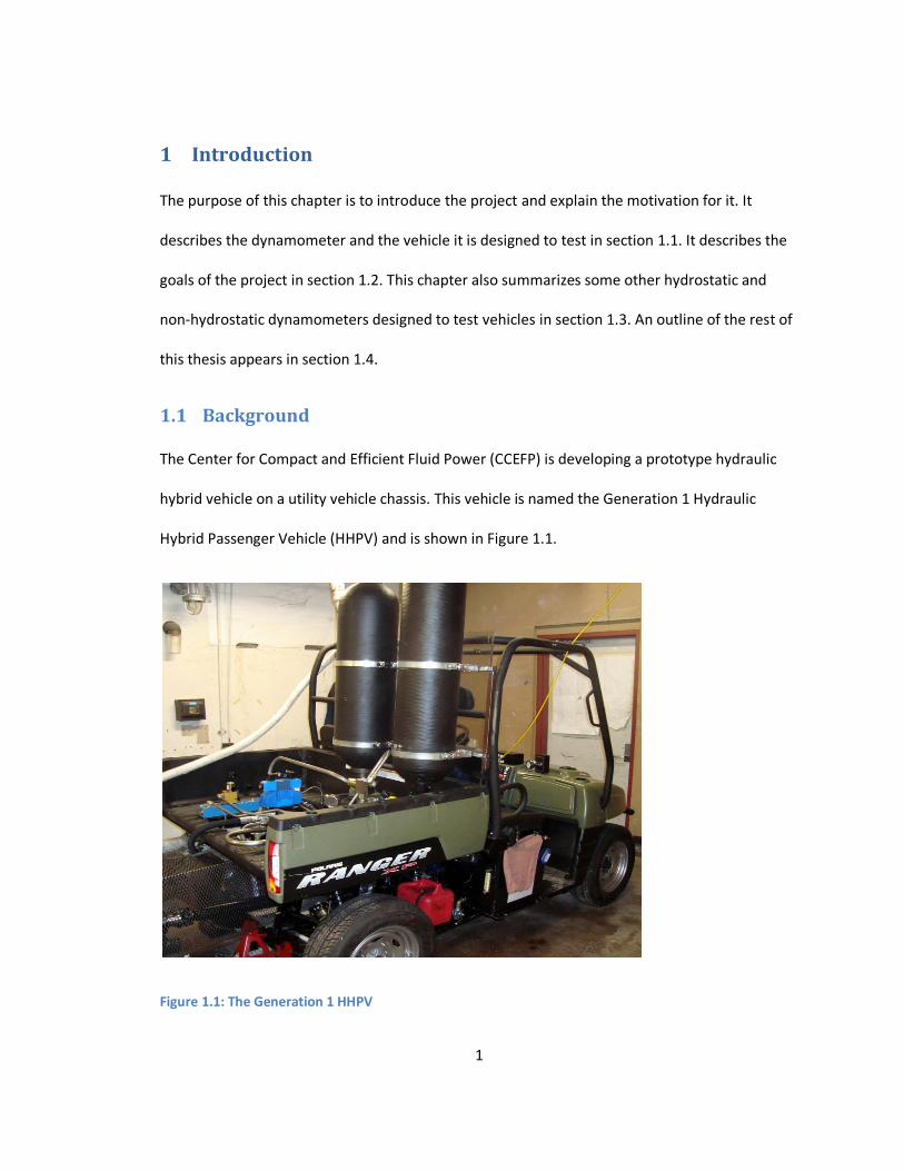
The Center for Compact and Efficient Fluid Power (CCEFP) is developing a prototype hydraulic
hybrid vehicle on a utility vehicle chassis. This vehicle is named the Generation 1 Hydraulic
Hybrid Passenger Vehicle (HHPV) and is shown in Figure 1.1.
Figure 1.1: The Generation 1 HHPV
2
The goal of this project is to demonstrate fuel savings by using a hydraulic hybrid powertrain.
Simulations show that fuel economies of over 60 miles per gallon are possible from this
particular vehicle.
A hybrid vehicle stores energy from braking and when power demanded at the wheels is less
than what the engine is able to produce. It releases this energy during acceleration when
demand peaks to supplement engine power. This allows the engine to be downsized. In a hybrid
vehicle, the engine can be sized to produce the average power requirement rather than the
highest power necessary for driving. The engine operates with increased efficiency because it
produces close to its peak power during most of its duty cycle.
Hybrid vehicles commonly store energy in two ways: electrically or hydraulically. Electric hybrids
store energy in batteries and are commonly available as passenger vehicles. Hydraulic hybrids
store energy by compressing a gas in an accumulator. Hydraulic components offer greater
power density than electric components, but the energy storage density of hydraulic
accumulators is less than that of batteries. Therefore, a limited selection of commercially
available hydraulic hybrid heavy trucks exists, but the technology has not yet penetrated the
passenger vehicle market.
Hydraulic hybrid powertrains can be built in three classes of configurations: series, parallel, and
power split. Each configuration requires an accumulator to store energy. In the series
configuration, the engine drives a pump which sends fluid to spin a motor connected to the
wheels. The engine is not mechanically linked to the wheels. This configuration loses energy as a
result of the transmission of all energy through hydraulics. The advantage of this architecture is
that it allows for excellent engine management with a simple control strategy [1]. In the parallel
configuration, the engine drives the wheels directly through a driveshaft, and a single pump
3
motor is coupled to the driveshaft. This configuration offers excellent power transmission
efficiency, but the engine does not operate at its most efficient point. For example, Stecki et al.
[2] implemented a parallel hydraulic hybrid system in a Freightliner truck. Using hydraulic power
to supplement engine power at the wheels, they achieved an average 37% fuel savings on an
urban drive cycle.
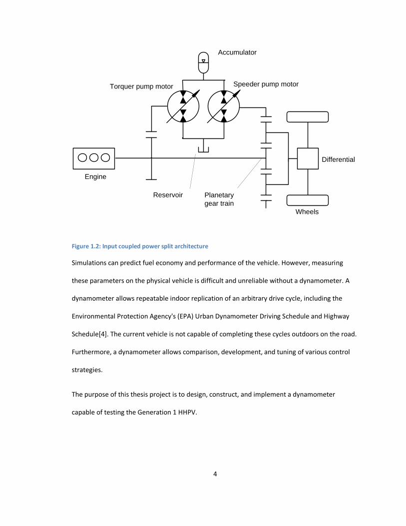
The CCEFP has chosen to pursue an "input coupled" power split configuration [3]. A block
diagram appears in Figure 1.2. A planetary gear train splits engine power to travel both through
hydraulics and a driveshaft. The "torquer" pump motor is geared directly to the engine, and its
displacement can be varied to change the torque on the engine. The "speeder" pump motor is
connected to the engine and wheels through a planetary gear train, and its displacement can be
varied to change their speed. Engine management improves because the engine speed does not
depend directly on wheel speed, yet transmission losses are reduced because some of the
power travels through a driveshaft. Little practical demonstration of the power split architecture
in a hydraulic hybrid passenger vehicle exists, so the CCEFP is building a prototype vehicle and
creating simulations based on this hardware. The power split architecture also allows fuller
control flexibility than the series or parallel architectures.
4
Engine
Wheels
Accumulator
Differential
Torquer pump motor Speeder pump motor
Planetary
gear train
Reservoir
Figure 1.2: Input coupled power split architecture
Simulations can predict fuel economy and performance of the vehicle. However, measuring
these parameters on the physical vehicle is difficult and unreliable without a dynamometer. A
dynamometer allows repeatable indoor replication of an arbitrary drive cycle, including the
Environmental Protection Agency's (EPA) Urban Dynamometer Driving Schedule and Highway
Schedule[4]. The current vehicle is not capable of completing these cycles outdoors on the road.
Furthermore, a dynamometer allows comparison, development, and tuning of various control
strategies.
The purpose of this thesis project is to design, construct, and implement a dynamometer
capable of testing the Generation 1 HHPV.
5
1.2 Requirements and goals
The main goal of dynamometer testing is to mimic outdoor driving in a controlled indoor
environment. Fuel economy can be measured and compared to that of other vehicles on a
standard drive cycle. Although possible, outdoor road testing is difficult and not repeatable.
Dynamometer testing eliminates variables from outdoor testing such as wind, weather, tire
pressure, and traffic. The dynamometer loads (absorbs power from) the vehicle's powertrain as
though it is driving. This dynamometer must also be able to motor (provide power back into) the
powertrain to replicate braking. The motoring feature is necessary to measure the vehicle's
effectiveness of capturing and storing braking energy.
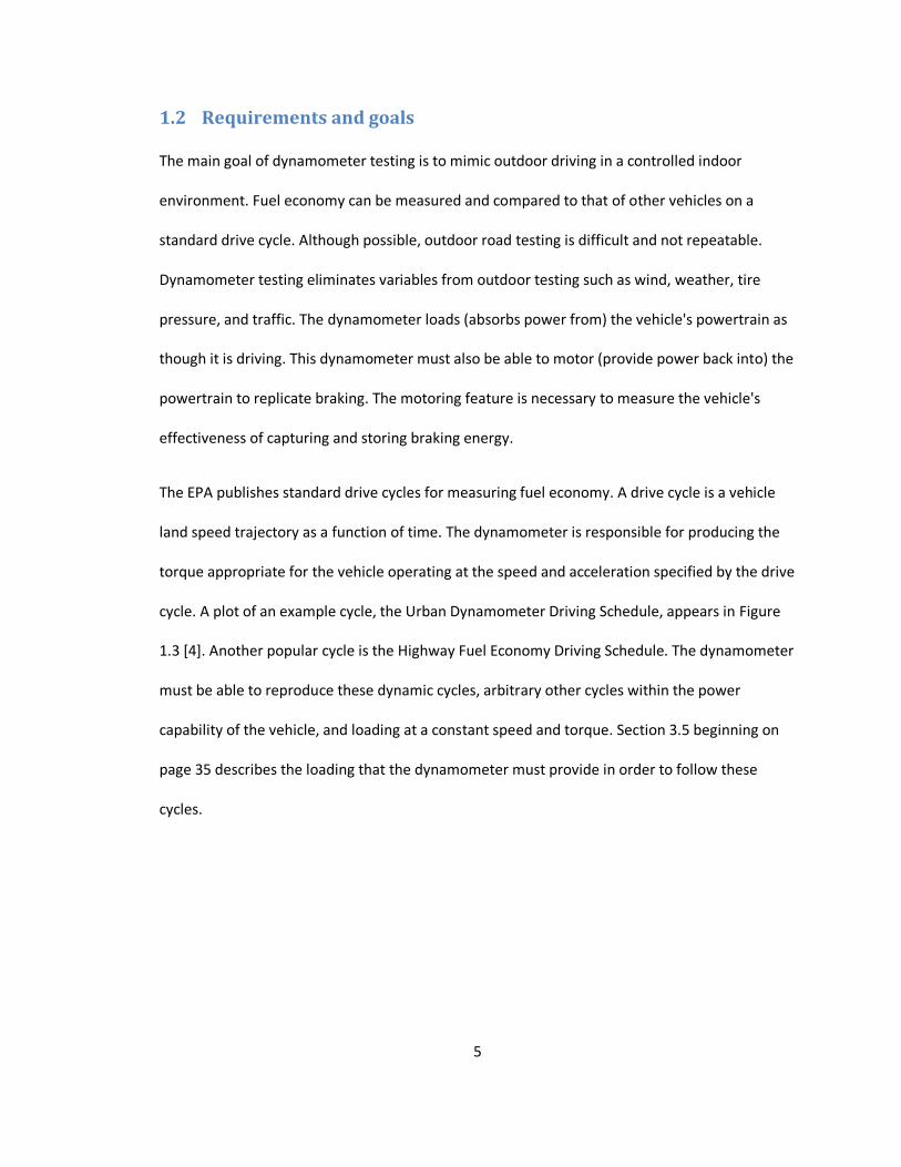
The EPA publishes standard drive cycles for measuring fuel economy. A drive cycle is a vehicle
land speed trajectory as a function of time. The dynamometer is responsible for producing the
torque appropriate for the vehicle operating at the speed and acceleration specified by the drive
cycle. A plot of an example cycle, the Urban Dynamometer Driving Schedule, appears in Figure
1.3 [4]. Another popular cycle is the Highway Fuel Economy Driving Schedule. The dynamometer
must be able to reproduce these dynamic cycles, arbitrary other cycles within the power
capability of the vehicle, and loading at a constant speed and torque. Section 3.5 beginning on
page 35 describes the loading that the dynamometer must provide in order to follow these
cycles.
6
Figure 1.3: EPA's Urban Dynamometer Driving Schedule[4]
Other limitations added additional requirements for the dynamometer. The vehicle and
dynamometer needed to fit in a 5 by 6m space. It is on the fourth floor of a building, and the
floor and doorway could not be modified. Therefore, all components needed to fit in an
elevator, through a doorway, and in the room. The room has exhaust ventilation, tap water, and
three phase 20A power available. Adding additional utilities such as chilled water or a high
current power supply would cost tens of thousands of dollars. The project's materials budget is
$5,000. Dynamometer operators are graduate students; new students must be able to quickly
learn how to use it safely.
1.3 Literature review
This section outlines the EPA fuel economy test procedure the dynamometer is intended to
follow. It also summarizes some other hydrostatic and non-hydrostatic dynamometers used in
similar applications.
1.3.1 EPA procedure
The EPA publishes a thorough procedure for evaluating vehicle fuel economy in the Code of
Federal Regulations [5]. Vehicles complete the Urban Dynamometer Driving Schedule to receive
7
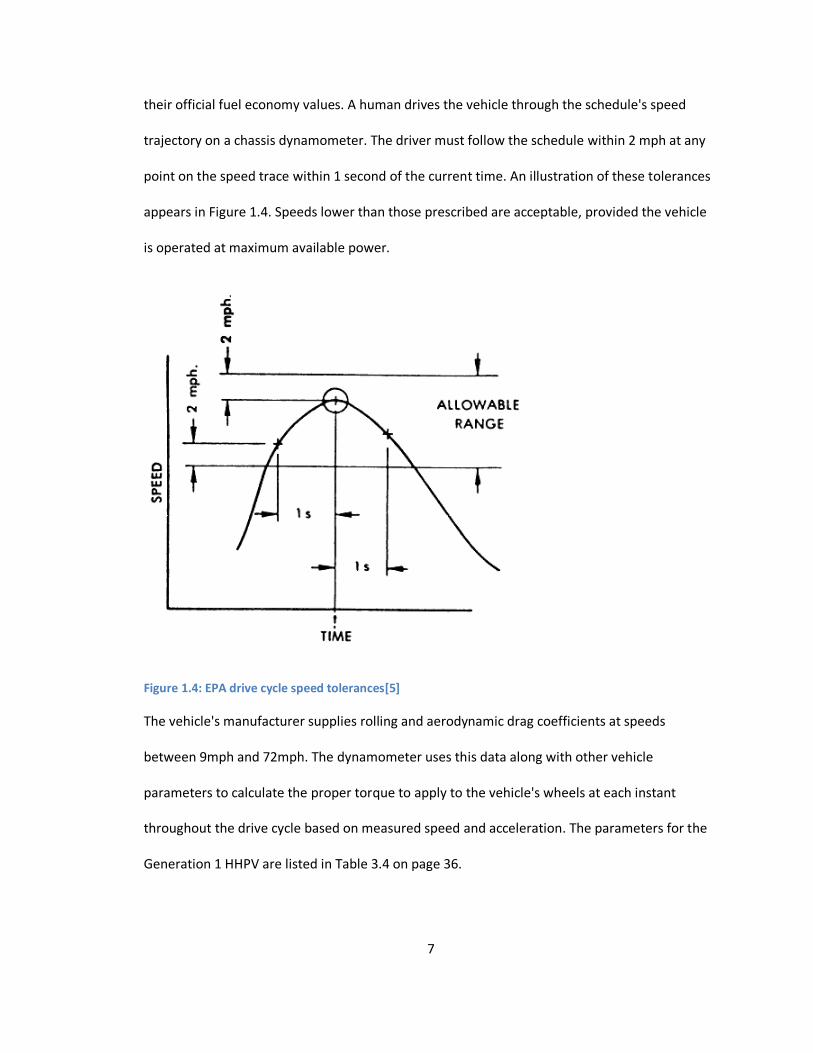
their official fuel economy values. A human drives the vehicle through the schedule's speed
trajectory on a chassis dynamometer. The driver must follow the schedule within 2 mph at any
point on the speed trace within 1 second of the current time. An illustration of these tolerances
appears in Figure 1.4. Speeds lower than those prescribed are acceptable, provided the vehicle
is operated at maximum available power.
Figure 1.4: EPA drive cycle speed tolerances[5]
The vehicle's manufacturer supplies rolling and aerodynamic drag coefficients at speeds
between 9mph and 72mph. The dynamometer uses this data along with other vehicle
parameters to calculate the proper torque to apply to the vehicle's wheels at each instant
throughout the drive cycle based on measured speed and acceleration. The parameters for the
Generation 1 HHPV are listed in Table 3.4 on page 36.
8
Reference [5] also specifies a procedure for preparing the vehicle for the test. It includes
instructions on fueling, temperature, and emissions measurement. Depending on the test being
run, the vehicle may be warmed, driven, and filled with a precise volume of fuel prior to testing.
1.3.2 Construction of other hydrostatic dynamometers
The following papers describe construction of custom hydrostatic dynamometers for various
purposes.
Rolewicz [6] built a system of hydrostatic dynamometers to test various components of a four-
wheel drive military vehicle. It used pumps to absorb power from components and a servovalve
controlled hydraulic motor to provide input power to the components that were not self-
powered. This project required a modular and compact solution to allow interchanging of
various components under test. It considered other types of dynamometers but settled on a
hydrostatic variety because the low inertia and high stiffness improve controllability. The project
reduced costs by reusing existing components. Rolewicz [6] is an example of a similar project
that selected the hydrostatic option in order to reduce cost. The hydrostatic advantage of robust
capabilities to pump and motor a large variety of equipment is appealing, although the current
project is purpose built for a specific vehicle.
Longstreth et al. [7] build off of the work in [6]. Its goal was to realize a cost effective high-
bandwidth dynamometer capable of producing transient torques. It used a fixed displacement
pump coupled to a servovalve to control load. The low inertia of the pump compared to
traditional dynamometers improved bandwidth and reduced vibrations. This paper shows that a
hydrostatic dynamometer is a good choice for transient loading, which the current project
requires.
9
Wang et al. [8] constructed a hydrostatic engine dynamometer to emulate the dynamics of a
hybrid powertrain. The power density, low inertia, and high bandwidth are listed as reasons that
"the hydrostatic dynamometer is an ideal candidate for the next-generation dynamometers." It
could motor the engine when no combustion is occurring. A variable displacement pump was
connected to the engine under test. A proportional valve and load sensing compensator
controlled the load with fast tracking.
Holland et al. [9] built a low-cost absorbing hydrostatic dynamometer to test small and medium
sized engines for educational purposes. It used a fixed displacement pump and proportional
relief valve to control load; it did not offer motoring capabilities. The high power density of
hydraulic systems allowed the dynamometer to be portable. It was durable and easy for
inexperienced operators to learn to use.
Like this project, many of the previous papers identified low cost, low inertia, and high power
density as advantages of hydrostatic dynamometers. The major disadvantage compared to
electric dynamometers is that they are not an established commercial product and must be
custom built.
1.3.3 Related work
Hydrostatic dynamometers are far from the only viable option for testing hybrid vehicles.
Nowell used a dynamometer with inertia weights and a hydro-viscous absorber to test trucks on
the EPA Federal Test Procedure duty cycle [10]. The inertial flywheels allow motoring without a
driving power device. The truck drives the dynamometer either through its driveshaft or a single
wheel. Although the approach is different, the goals and configuration of this is similar to those
of the current project.
10
Wilson [11] constructed an eddy current chassis dynamometer to test a racecar and other
vehicles. The vehicle drove on rollers loaded by an eddy current dynamometer. See subsection
3.3.2 for a description of eddy current technology. Wilson elected to construct his own roller
apparatus to reduce cost.
1.4 Overview
Chapter 2 describes the final dynamometer: its physical construction, electronics, controls,
sensors, and safety features. Chapter 3 describes the design process which used computer
models to guide component selection. Chapter 0 presents the experimentally observed
performance of the dynamometer. Chapter 5 concludes the thesis and presents possible future
work and opportunities for the dynamometer. Appendix A contains a bill of materials for the
dynamometer. Appendix B contains electrical schematics. Appendix C contains instructions for
calibrating the torque sensor. Appendix D contains the MATLAB code used for design. Appendix
E shows a portion of the Simulink model used for controller design. Appendix F contains
operating instructions for the dynamometer.
11
2 Description of Final Physical Dynamometer
This chapter describes the physical dynamometer and how it works. It presents a high level
overview of the dynamometer's method of operation in section 2.1. A hydraulic schematic of
the dynamometer is presented, and each component is explained in section 2.2. The physical
configuration of the machine is described in section 2.3. The electrical system is described along
with the manual and automatic methods of controlling the dynamometer in sections 2.4, 2.5,
and 2.6. Sensors and the data acquisition are described in sections 2.7 and 2.8. Safety features
and ergonomics are explained in sections 2.9 and 2.10. Cost reduction techniques are described
in section 2.11.
2.1 Overview of operation
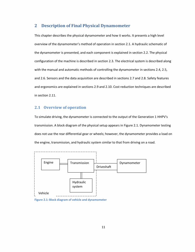
To simulate driving, the dynamometer is connected to the output of the Generation 1 HHPV's
transmission. A block diagram of the physical setup appears in Figure 2.1. Dynamometer testing
does not use the rear differential gear or wheels; however, the dynamometer provides a load on
the engine, transmission, and hydraulic system similar to that from driving on a road.
Vehicle
Engine Transmission Dynamometer
Hydraulic system
Driveshaft
Figure 2.1: Block diagram of vehicle and dynamometer
12
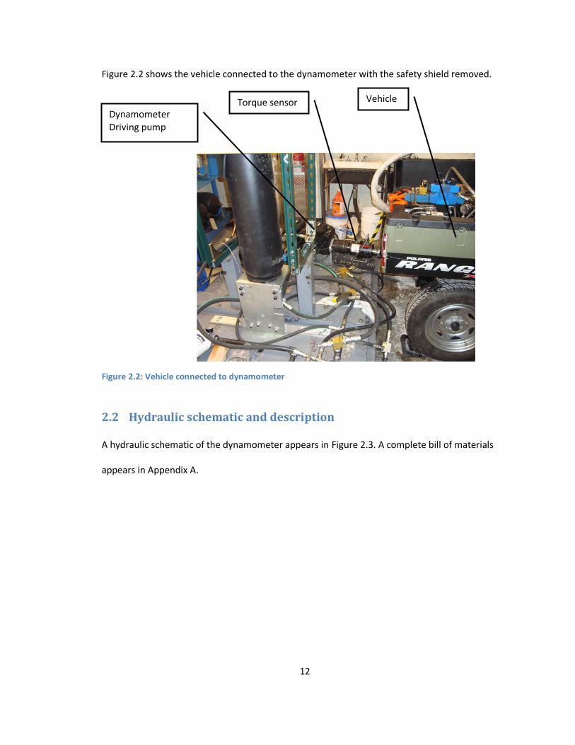
Figure 2.2 shows the vehicle connected to the dynamometer with the safety shield removed.
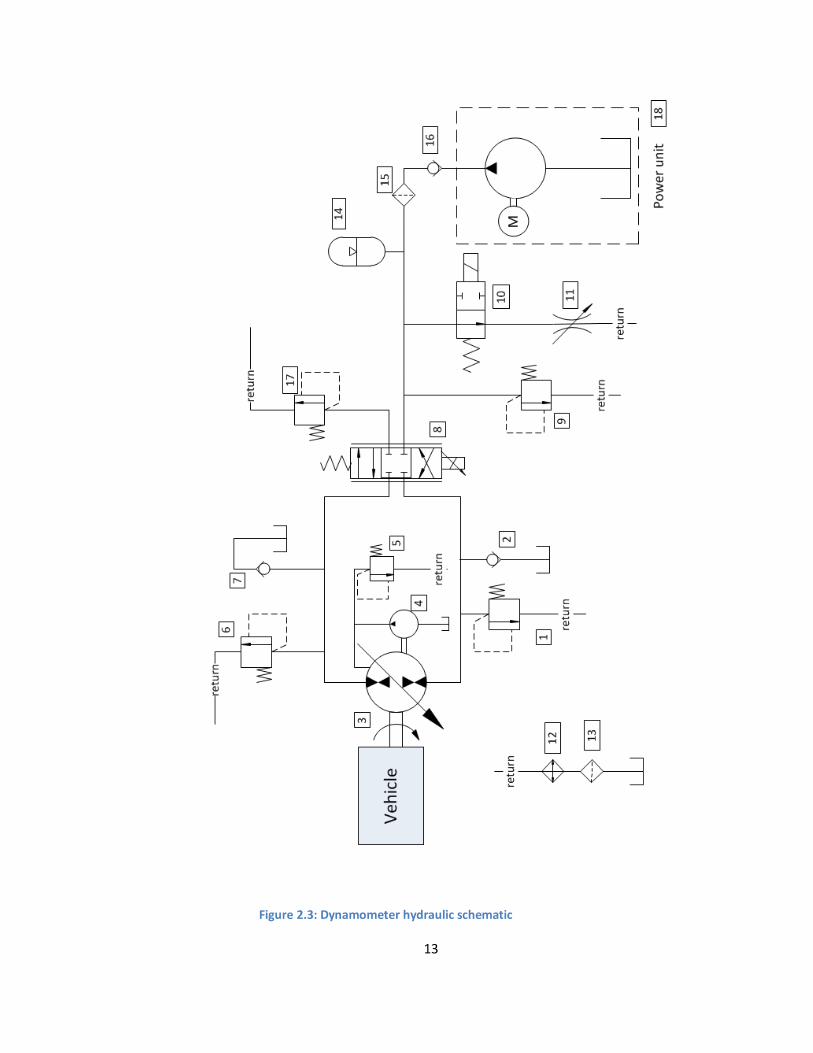
2.2 Hydraulic schematic and description
A hydraulic schematic of the dynamometer appears in Figure 2.3. A complete bill of materials
appears in Appendix A.
Dynamometer Driving pump
Torque sensor Vehicle
Figure 2.2: Vehicle connected to dynamometer
13
Figure 2.3: Dynamometer hydraulic schematic
14
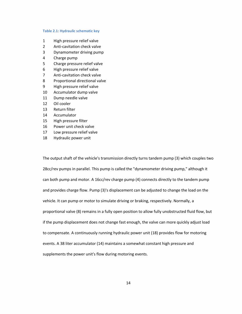
Table 2.1: Hydraulic schematic key
1 High pressure relief valve
2 Anti-cavitation check valve
3 Dynamometer driving pump
4 Charge pump
5 Charge pressure relief valve
6 High pressure relief valve
7 Anti-cavitation check valve
8 Proportional directional valve
9 High pressure relief valve
10 Accumulator dump valve
11 Dump needle valve
12 Oil cooler
13 Return filter
14 Accumulator
15 High pressure filter
16 Power unit check valve
17 Low pressure relief valve
18 Hydraulic power unit
The output shaft of the vehicle's transmission directly turns tandem pump (3) which couples two
28cc/rev pumps in parallel. This pump is called the "dynamometer driving pump," although it
can both pump and motor. A 16cc/rev charge pump (4) connects directly to the tandem pump
and provides charge flow. Pump (3)'s displacement can be adjusted to change the load on the
vehicle. It can pump or motor to simulate driving or braking, respectively. Normally, a
proportional valve (8) remains in a fully open position to allow fully unobstructed fluid flow, but
if the pump displacement does not change fast enough, the valve can more quickly adjust load
to compensate. A continuously running hydraulic power unit (18) provides flow for motoring
events. A 38 liter accumulator (14) maintains a somewhat constant high pressure and
supplements the power unit's flow during motoring events.
15
Valves (1), (2), (6), and (7) prevent cavitation and trapped pressure when valve (8) is in the
center position. A relief valve (9) is redundant to the power unit's internal relief valve but can
accommodate the higher flow rate that the accumulator (14) or dynamometer driving pump (3)
are capable of producing. Normally open solenoid valve (10) dumps the accumulator's stored
energy if the operator presses the emergency stop button or if electrical power is lost.
Low pressure filter (13) and high pressure filter (15) remove contamination from both the pump
and return lines. Filter (15) does not meet the cleanliness requirements of the proportional
valve, but filter (13) does. The proportional valve requires a 3 micron or finer filter. The heat
exchanger (12) cools the hot oil by passing its heat to tap water. The warm water drains to the
sewer.
During normal loading, the dynamometer driving pump (3) draws fluid through a check valve (2
or 7, depending on flow direction) from the tank via suction. The fluid is pressurized by the
dynamometer driving pump and pumped through a relief valve (1 or 6). The fluid passes through
the low pressure filter (13) and oil cooler (12) before returning to the tank.
2.2.1 Description of hydraulic components
The following subsections describe each of the components in the above hydraulic schematic in
more detail.
2.2.1.1 Dynamometer driving pump (3)
The dynamometer driving pump is directly connected to the driveshaft exiting the vehicle's
transmission. It can absorb power or motor. It consists of two 28cc/rev Sauer-Danfoss Series 42
axial piston pumps coupled together in a tandem configuration. The shaft only spins in one
direction. The pump's displacement can be varied infinitely from full to negative full, allowing
16
bidirectional flow. The pump's displacement is proportional to the electrical command current
between 14 and 85mA. A negative command current corresponds to negative displacement.
2.2.1.2 Hydraulic power unit (18)
The power unit runs continuously to fill the accumulator and provide flow for motoring. It is a
model J-8985 assembled by Air Hydraulic Systems and can provide about 19LPM at 200bar. It
has been modified to add a suction line and the capacity for more flow to prevent excessive
pressure drops. A directional valve was removed, and the pressure line was connected directly
to the dynamometer. All return oil passes through a single separate filter and oil cooler. The
power unit's original return line filter was removed and replaced with one capable of meeting a
higher cleanliness rating and flow rate. The new filter is described in subsection 2.2.1.10. The
power unit did not have an available suction line, so one was installed for the charge pump (4)
and check valves (2 and 7) using a pipe inserted through a new hole in the top of the reservoir.
After passing through a Mueller Steam Specialty 20 micron Y type strainer (not shown in the
schematic), the suction flow passes through a suction hose. A filter is not installed in the suction
line to reduce the risk of cavitation. The hydraulic fluid is Mobil DTE 25.
2.2.1.3 Accumulator (14)
A Parker BA 38 liter bladder accumulator maintains a somewhat constant high pressure. If the
dynamometer driving pump (3) requires more power than the power unit can provide while
motoring, the accumulator supplements its flow. The accumulator fills when the dynamometer
driving pump is pumping.
2.2.1.4 Proportional valve (8)
The proportional valve can vary the load faster than by changing the dynamometer driving
pump's displacement. The manufacturer advertises a 50ms response time [12, p. 4]. The valve is
an Eaton KFDG5V-7 two stage proportional directional valve rated for flows up to 160LPM. Its
17
amplifier is in the dynamometer's power box. The amplifier receives a signal from the controller
and feedback from the valve's spool position sensor. It sends current to the valve's solenoid. A
reducing valve (not shown in schematic) is sandwiched between the main and pilot stage to
provide pilot pressure by reducing the main system pressure to about 30bar. Pilot pressure from
this valve is separate from the pump's charge pressure.
2.2.1.5 Charge pump(4) and relief valve (5)
The charge pump connects to the tandem dynamometer driving pump. It is a Hydreco HMP3
162025A2 16cc/rev gear pump. The relief valve is set to maintain charge pressure at about
14bar, as required by the manufacturer of the dynamometer driving pump [13, p. 9]. A reducing
valve had been used to supplement charge flow during startup, but the reducing valve is
excluded from the final design to prevent the dynamometer from motoring in reverse. See
section 5.3 for more information.
2.2.1.6 Relief valve (17)
An Eaton RV5-10 cartridge relief valve maintains the low pressure at about 14bar. Without this
minimal backpressure, the dynamometer driving pump's charge flow consumption increases
substantially, and the charge pump is unable to keep up. Only return oil from the dynamometer
driving pump passes through this valve.
2.2.1.7 Relief valves (1 and 6) and check valves (2 and 7)
When proportional valve (8) is not throttling flow (the spool is at an end position), these check
and relief valves remain closed. When the proportional valve is throttling and the dynamometer
driving pump is pumping, one check valve opens to prevent cavitation. The relief valve may also
open on the opposite side if the pressure reaches the maximum system pressure. For example,
if directional valve (8) is closed and the dynamometer driving pump (3) is pumping flow in the
counterclockwise direction, check valve (7) and relief valve (1) open. One check valve is a Parker
18
C-2020-S in-line check valve; the other is an Eaton CV1-16 cartridge check valve. Both relief
valves are Eaton RV5-10 cartridge relief valves. Relief pressures are set to the maximum system
pressure of 200bar.
Check valve (16)
A Sun Hydraulics CXDA-XAN cartridge check valve prevents flow from the accumulator (14) from
spinning the power unit backwards after it is shut off and prevents reverse flow through the
high pressure filter (15).
2.2.1.8 Relief valve (9)
This Eaton RV5-10 cartridge relief valve relieves flow from the dynamometer driving pump (3)
and power unit when the accumulator is full. Although the power unit also has an internal relief
valve, it is not designed for the high flows that the dynamometer driving pump can produce. The
new relief valve is capable of relieving 114LPM at 200bar.
2.2.1.9 Dump valve (10) and needle valve (11)
Dump valve (10) is a normally open Eaton SV13-16-O solenoid cartridge valve. Needle valve (11)
is a Sun Hydraulics NFCC needle valve. The dump valve is energized and closed when the
dynamometer is operating normally. When the operator presses the emergency stop button or
if power is lost, the dump valve opens, releasing the accumulator's stored energy. The needle
valve prevents the flow exiting the accumulator from being too fast; it must be adjusted upon
installation and periodically to provide the desired flow rate to empty the accumulator in about
10s. A fixed orifice will replace the needle valve in the future so that it cannot be closed.
2.2.1.10 Filters 13, 15
The proportional valve (8) is the most sensitive component in the system to contamination and
requires an ISO cleanliness level of 18/16/13 [12, p. 16]. The valve's manufacturer recommends
that a filter be installed upstream of proportional valves [14]. The high pressure Eaton HF2P
19
filter (15) does not meet the ISO cleanliness level for the valve, so a Parker 50AT return line filter
(13) is also used. The return line filter has a pressure gauge to measure backpressure. The filter
element should be replaced with a Parker 926541 canister when backpressure exceeds 1.7bar or
after 250 hours of service.
2.2.1.11 Oil cooler (12)
Energy from the vehicle is converted to heat by throttling fluid. All return oil passes through this
oil cooler and filter (13). The Thermasys EKS shell and tube heat exchanger removes up to 15kW
of heat from the oil to a continuously running cold water supply. The warm water is dumped to
the sewer. A solenoid water valve shuts off the water flow automatically when the
dynamometer is shut down, but it is good practice to manually close the gate valve on the water
supply as well to reduce leaks.
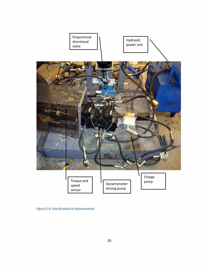
2.3 Physical design
Figure 2.4 shows a photograph of the physical dynamometer.
20
Figure 2.4: Overall physical dynamometer
Dynamometer driving pump
Charge pump Torque and
speed sensor
Hydraulic power unit
Proportional directional valve
21
Most components rest on a concrete bedplate. The dynamometer driving pump is supported by
a commercially available foot bracket, which is connected to the bedplate with concrete
anchors. The bladder accumulator must be held vertically according to the manufacturer's
instructions. The top of the accumulator is supported by a strut and plywood structure; the
bottom sits in a commercially available base. Valves and other lightweight components simply
rest on the bedplate.
Most of the fluid connectors are hose with JIC fittings, but the low pressure and suction lines use
some pipe. Although rigid steel tubing offers many advantages, it is impractical for this project.
Since this is a prototype project, hose offers the flexibility to move or change components
without replacing a tube. Plastic tubing connects the oil cooler to the city cold water and sewer
at a nearby sink.
A hydraulic power unit on wheels is parked next to the bedplate. The rear of the vehicle is
positioned facing the dynamometer driving pump near the edge of the bedplate.
A rubber isolated tube style driveshaft supplied by Machine Service, Inc. connects the vehicle to
a torque and speed sensor (see section 2.7), which measures the torque and speed at the
vehicle's output shaft. The second shaft on the torque sensor connects to the dynamometer
driving pump.
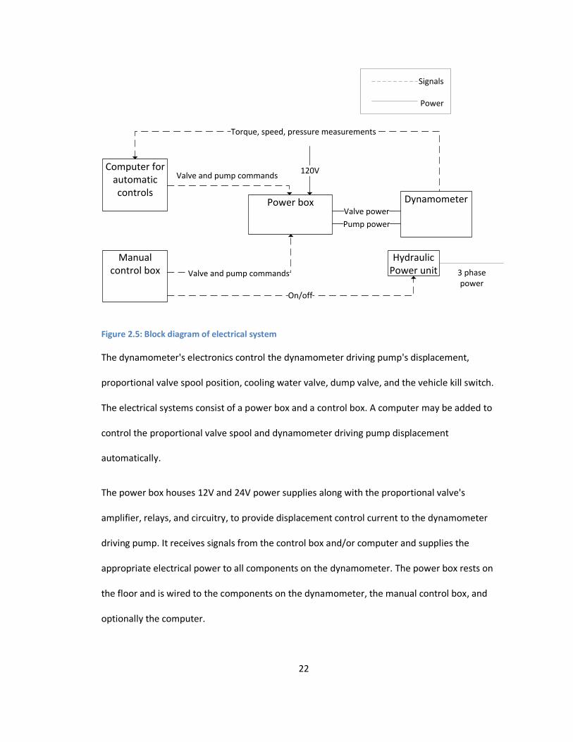
2.4 Power and electronics
A high level block diagram of the electrical schematic appears in Figure 2.5. Full electrical
schematics appear in Appendix B.
22
Computer for automatic controls
Manual control box
Power box Dynamometer
Hydraulic Power unitValve and pump commands
On/off
3 phase power
Pump power
Valve power
120V
Signals
Power
Torque, speed, pressure measurements
Valve and pump commands
Figure 2.5: Block diagram of electrical system
The dynamometer's electronics control the dynamometer driving pump's displacement,
proportional valve spool position, cooling water valve, dump valve, and the vehicle kill switch.
The electrical systems consist of a power box and a control box. A computer may be added to
control the proportional valve spool and dynamometer driving pump displacement
automatically.
The power box houses 12V and 24V power supplies along with the proportional valve's
amplifier, relays, and circuitry, to provide displacement control current to the dynamometer
driving pump. It receives signals from the control box and/or computer and supplies the
appropriate electrical power to all components on the dynamometer. The power box rests on
the floor and is wired to the components on the dynamometer, the manual control box, and
optionally the computer.
23
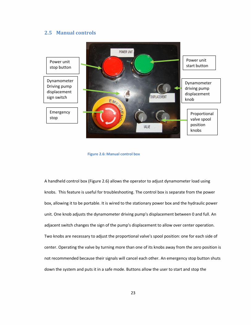
2.5 Manual controls
A handheld control box (Figure 2.6) allows the operator to adjust dynamometer load using
knobs. This feature is useful for troubleshooting. The control box is separate from the power
box, allowing it to be portable. It is wired to the stationary power box and the hydraulic power
unit. One knob adjusts the dynamometer driving pump's displacement between 0 and full. An
adjacent switch changes the sign of the pump's displacement to allow over center operation.
Two knobs are necessary to adjust the proportional valve's spool position: one for each side of
center. Operating the valve by turning more than one of its knobs away from the zero position is
not recommended because their signals will cancel each other. An emergency stop button shuts
down the system and puts it in a safe mode. Buttons allow the user to start and stop the
Figure 2.6: Manual control box
Proportional valve spool position knobs
Dynamometer driving pump displacement knob
Power unit start button
Power unit stop button
Dynamometer Driving pump displacement sign switch
Emergency stop
24
hydraulic power unit remotely. The original start/stop buttons remain in place on the power
unit.
2.6 Automatic controls
Two personal computers running xPC Target from MathWorks control the dynamometer
automatically. The user creates a block diagram controller on the host computer running
Windows XP and downloads it on to the target computer, which has no operating system. The
target computer contains the data acquisition and voltage output cards. It controls the
dynamometer in real time. The user can change some basic controller parameters while the real
time program is running from the host computer.
The purpose of the automatic controller is to control the dynamometer driving pump's
displacement and the proportional valve's spool position to provide the appropriate torque
based on the vehicle's speed. Inputs to the controller are driveshaft speed and dynamometer
driving pump torque and pressure. Outputs are dynamometer driving pump displacement and
proportional valve position. The controller is currently a proportional integrator (PI) with
feedforward. The feedforward portion calculates the dynamometer driving pump displacement
that theoretically produces the desired torque. The PI portion of the controller compares actual
to desired torque to correct the displacement command from the feedforward portion. This
controller currently leaves the proportional directional valve in its fully open position. However,
control of the proportional valve could be added later if the dynamic response needs to be
improved.
The manual control box has two electrical connectors. The first is for the emergency stop and
hydraulic power unit signals. The second is for the proportional directional valve and
25
dynamometer driving pump displacement signals. The cable for the first always remains
connected. The cable for the second can be removed from the manual control box and
connected through the computer for automatic controls.
2.7 Sensors
Sensors on the dynamometer measure pressure at both ports of the dynamometer driving
pump, driveshaft torque, and driveshaft speed. Omega PX309 pressure transducers are screwed
directly into the gauge ports of the dynamometer driving pump and are able to measure 210bar.
They output a voltage proportional to pressure which is read by the target PC's data acquisition
(DAQ) system. A Honeywell Lebow 1105 torque sensor placed between the dynamometer
driving pump and the driveshaft from the vehicle measures torque at this point. It is a strain
gauge based torque sensor with a slip ring. The electronics that modify the torque sensor's
signal for use by the DAQ system must be calibrated regularly. Calibration instructions appear in
Appendix C. The torque sensor unit also contains a speed sensor. It outputs 60 pulses per
revolution, so the frequency of pulses increases with speed.
Most of the sensing hardware was reused from a pump test stand developed to quantify the
performance of pump motors in the HHPV. A detailed explanation of the electronics necessary
to allow the sensors to communicate with the computer appears in Chapter 2 of reference[15].
2.8 DAQ system
Three Measurement Computing DAQ cards are installed in the target computer. A PCI-QUAD04
quadrature in card reads pulses from the speed sensor. A PCI-DAS1602/12 analog in card reads
analog signals from the pressure transducers and torque sensor. A PCI-DAC6702 analog out card
sends analog voltage commands to control the pump displacement and proportional valve. A
26
block for each of the DAQ cards is inside of the controller's Simulink block diagram. It allows
access to the DAQ cards' signals.
2.9 Safety features
Operation of the dynamometer presents many safety hazards including high pressure, high
temperature, external oil leaks, exhaust, noise, diesel fuel, potential flooding, stored energy,
tripping hazards, ergonomics, electrical hazards, and rotating machinery.
The dynamometer may be operated from a separate room that adjoins the test cell, mitigating
many of the above safety issues. The operator carries the control box into the adjacent room
and views the apparatus through a window. The computer for automatic control is on an
ergonomic cart and can be adjusted for either a standing or seated operator.
When the operator pushes the emergency stop button on the control box, the dynamometer
and vehicle lose power and go into a safe mode. The vehicle turns off, and its main power is cut.
The dynamometer also loses power, so the dynamometer driving pump's displacement becomes
zero. The dump valve (item 10 in Figure 2.3) opens and empties the accumulator's stored
energy. The operator does need to push the power unit's off button to shut this off separately.
The dynamometer is designed so that it cannot turn the vehicle's driveshaft backwards, which
could damage the engine. If the driveshaft began to turn backwards, the charge pump would
stop providing charge pressure. Thus, the dynamometer driving pump displacement would go to
zero, and the dynamometer would stop producing torque.
Exhaust exits the room through a sealed pipe. A large blower replaces the room's entire volume
of air once per minute, removing the small amount of exhaust gas that may leak. A fiberglass
sleeve encircles the exhaust tube to prevent anyone who touches it from burning themselves.
27
All rotating components, including the driveshaft, are shielded with expanded metal guards.
Electrical wires and tubes that run across a walk path are taped to the floor and marked with
hazard tape. All electrical connectors are mistake proof. No two connectors are the same type,
so it is impossible to improperly connect wires.
All high pressure fluid connectors are rated for at least 200bar. Flexible hose is used rather than
rigid tubing to connect to pumps to minimize damage and leakage due to vibration. All fluid
connectors are tested to be free of leaks, as leaks would create a slipping hazard.
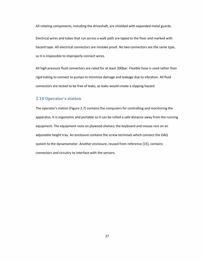
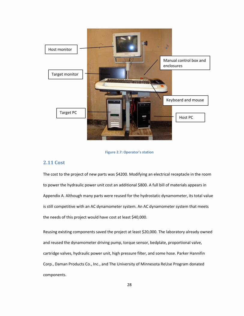
2.10 Operator's station
The operator's station (Figure 2.7) contains the computers for controlling and monitoring the
apparatus. It is ergonomic and portable so it can be rolled a safe distance away from the running
equipment. The equipment rests on plywood shelves; the keyboard and mouse rest on an
adjustable height tray. An enclosure contains the screw terminals which connect the DAQ
system to the dynamometer. Another enclosure, reused from reference [15], contains
connectors and circuitry to interface with the sensors.
28
Figure 2.7: Operator's station
2.11 Cost
The cost to the project of new parts was $4200. Modifying an electrical receptacle in the room
to power the hydraulic power unit cost an additional $800. A full bill of materials appears in
Appendix A. Although many parts were reused for the hydrostatic dynamometer, its total value
is still competitive with an AC dynamometer system. An AC dynamometer system that meets
the needs of this project would have cost at least $40,000.
Reusing existing components saved the project at least $20,000. The laboratory already owned
and reused the dynamometer driving pump, torque sensor, bedplate, proportional valve,
cartridge valves, hydraulic power unit, high pressure filter, and some hose. Parker Hannifin
Corp., Daman Products Co., Inc., and The University of Minnesota ReUse Program donated
components.
Target PC
Target monitor
Host monitor
Host PC
Keyboard and mouse
Manual control box and enclosures
29
Pipe fittings offer a cost savings over JIC fittings but sacrifice leak tightness and durability.
Therefore, pipe was used as a low cost fluid connector on low pressure return and suction lines
where the risk of leaks was not great. The maximum system pressure is 200bar (3000psi).
Although a 340bar (5000psi) system would have increased power density, 200bar components
cost less and are more available. Designing the system for the lower pressure saved weeks of
time and thousands of dollars.
30
3 Design
This chapter describes the design process followed to converge on the final product. Critical
requirements are summarized in section 3.1. A product design specification appears in section
3.2. Using contract testing services or purchased dynamometers was researched in section 3.3.
Eventually, a purpose built hydrostatic dynamometer was chosen using a product selection chart
in section 3.4. General component specifications were developed using MATLAB simulations. A
MATLAB simulation of the vehicle is described in section 3.5. Two different simulations of the
dynamometer were created for distinct purposes. Section 3.6 describes a MATLAB simulation of
the dynamometer made for the purpose of component sizing. A dynamic model of the
dynamometer was created in Simulink in section 3.7 for the purpose of controller design. Data
from these simulations is used to select or justify reusing components in section 3.8.
3.1 Summary of customer requirements
The purpose of the dynamometer is to test a hydraulic hybrid vehicle built on a Polaris Ranger
utility vehicle chassis. In order to replicate driving on the road and be feasible for this project,
the dynamometer must:
Be safe to operate.
Cost about $5000 in new components.
Follow EPA drive cycles, including portions requiring motoring.
Be in a convenient location to allow frequent testing.
3.2 Product design specification
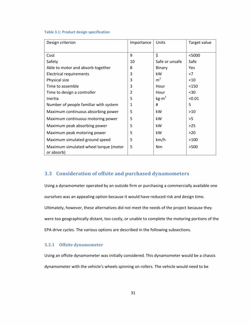
Table 3.1 summarizes the design specifications for the dynamometer. The importance of the
design criteria is ranked on a scale from 1 to 10.
31
Table 3.1: Product design specification
Design criterion Importance Units Target value
Cost 9 $ <5000
Safety 10 Safe or unsafe Safe
Able to motor and absorb together 8 Binary Yes
Electrical requirements 3 kW <7
Physical size 3 m2 <10
Time to assemble 3 Hour <150
Time to design a controller 2 Hour <30
Inertia 5 kg·m2 <0.01
Number of people familiar with system 1 # 5
Maximum continuous absorbing power 5 kW >10
Maximum continuous motoring power 5 kW >5
Maximum peak absorbing power 5 kW >25
Maximum peak motoring power 5 kW >20
Maximum simulated ground speed 5 km/h >100
Maximum simulated wheel torque (motor or absorb)
5 Nm >500
3.3 Consideration of offsite and purchased dynamometers
Using a dynamometer operated by an outside firm or purchasing a commercially available one
ourselves was an appealing option because it would have reduced risk and design time.
Ultimately, however, these alternatives did not meet the needs of the project because they
were too geographically distant, too costly, or unable to complete the motoring portions of the
EPA drive cycles. The various options are described in the following subsections.
3.3.1 Offsite dynamometer
Using an offsite dynamometer was initially considered. This dynamometer would be a chassis
dynamometer with the vehicle's wheels spinning on rollers. The vehicle would need to be
32
transported to an offsite location and connected to the dynamometer with minimal
modification.
Although the offsite dynamometer would have been the fastest to implement and lowest risk, it
was rejected because no dynamometers in close geographic proximity to the vehicle's location
in Minneapolis, MN met the needs of the project. Local dynamometers only offered the ability
to absorb power, not motor. The nearest available motoring chassis dynamometer was a 90
minute drive away in Mankato, MN and may not have been operational in time for the vehicle's
testing. The next available option was in Ann Arbor, MI, a 12 hour drive away. Both of these
options were too geographically distant to allow frequent testing and development work.
3.3.2 Purchased dynamometer
An AC or DC dynamometer contains a large electric motor/generator and is capable of both
motoring and absorbing power. Initial costs are high; the dynamometer alone costs $40000.
Furthermore, the room available for the vehicle testing would have required substantial work to
accommodate the electrical demands of the machine.
An eddy current dynamometer uses eddy currents in a large rotating metal disc to generate a
load. It would need to be combined with an electric motor to provide motoring power. This
project had access to an eddy current dynamometer but not the electric motor which would
have also required electrical modifications to the room.
3.4 Selection of general design
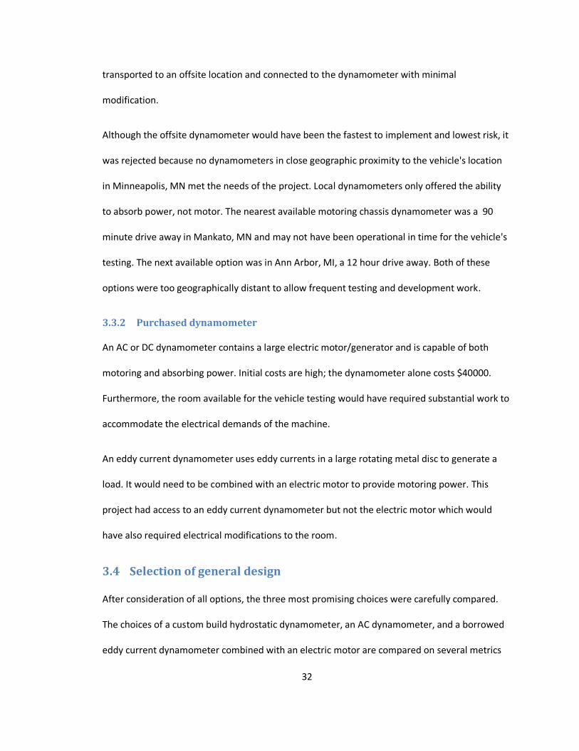
After consideration of all options, the three most promising choices were carefully compared.
The choices of a custom build hydrostatic dynamometer, an AC dynamometer, and a borrowed
eddy current dynamometer combined with an electric motor are compared on several metrics

33
in Table 3.2. The degree to which each of the three choices meets the needs of the project is
quantified in Table 3.3, and the hydrostatic dynamometer is deemed the best choice.
34
Table 3.2: Comparison of general dynamometer designs
Hydrostatic AC dynamometer Borrowed eddy current + electric motor
Cost $5000. $40000 plus electrical work.
$12000 plus electrical work.
Safety Lower than others. Unproven technology. Leaks. Stored energy in accumulator. Possible to drive transmission in wrong direction.
Medium. Some electrical and heat hazards. Possible to drive transmission in wrong direction.
Medium. Some electrical and heat hazards. Unlikely to drive transmission in wrong direction.
Able to motor and absorb together
Yes. Yes. No. Requires changing components to change between motoring and absorbing.
Probability of success
Successful in some papers but not commercially available.
Proven. Eddy current is proven. Motoring portion is unusual.
Electrical requirements
Minimal. Three phase only.
Most. Requires high current plus sending power back to grid.
Three phase. Possibly higher current required than hydrostatic.
Physical size Smallest. Medium. May require large drive cabinet.
Largest. Motor and dynamometer are separate.
Time to assemble Hardest. Entirely custom.
Easiest. Comes semi-assembled.
Medium.
Time to design a controller
Hardest. Multiple variables to control.
Easiest. Manufacturer provides a torque controller.
Easy. Motor drive and dynamometer have their own controllers.
Inertia Best. Medium. Medium.
Number of people familiar with system
Best. Many hydraulics experts available.
Worst. Medium. These are common in the engine lab but not in our group.
Max. simulated ground speed
Same as others Same as others Same as others
Max. simulated wheel torque
Same as others Same as others Same as others
35
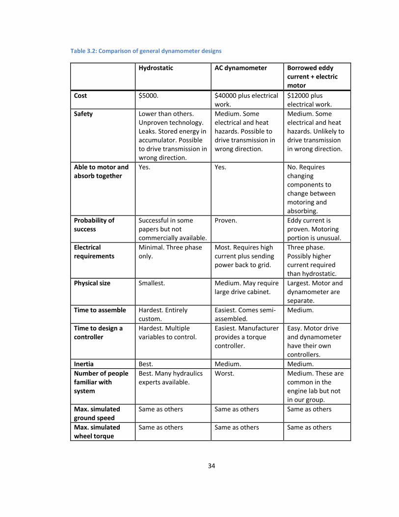
Table 3.3 quantifies the information in Table 3.2. Each design criterion is assigned a weight
ranging from 1 to 10. The degree to which each of the three design possibilities satisfies the
design criteria is rated on a scale ranging from 0 to 5. The ratings are multiplied by the weights
and summed for each of the three designs. The best design is the one with the most total points.
Maximum torque, speed, and power specifications are excluded because all options are equally
capable of meeting these specifications.
Table 3.3: Evaluation of design options
Design criterion Weight Hydro-static
AC Borrowed eddy current + electric motor
Cost 9 5 0 2 Safety 10 1 2 3 Able to motor and absorb together 8 5 5 1 Electrical requirements 3 4 0 2 Physical size 3 5 3 2 Time to assemble 3 1 5 3 Time to design a controller 2 1 5 4 Inertia 5 5 2 2 Number of people familiar with system 1 5 2 3
Total 157 106 98
The hydrostatic dynamometer received the most points and was selected for this project.
3.5 MATLAB simulation of vehicle
A simple MATLAB simulation was created to calculate loads experienced by the vehicle on an
arbitrary drive cycle. The output of the simulation is the wheel torque and wheel speed. The
code of this simulation appears in Appendix D.
EPA drive cycles provide speed data at a frequency of 1Hz. The simulation differentiates the
drive cycle's speed versus time information using a backward difference numerical derivative to
36
calculate the vehicle's acceleration. This method does not generate substantial noise for the EPA
drive cycles because the speed data is already smooth. The simulation calculates the force due
to acceleration by multiplying acceleration by the vehicle's mass. It calculates the rolling
resistance based on the vehicle's speed, weight, and rolling resistance coefficients. It calculates
drag force based on the vehicle's speed, frontal area, drag coefficient, and air density. It
calculates vehicle power by multiplying the speed by the total resistive force. It calculates the
rotational speed of the wheels by dividing the road speed by the tire radius.
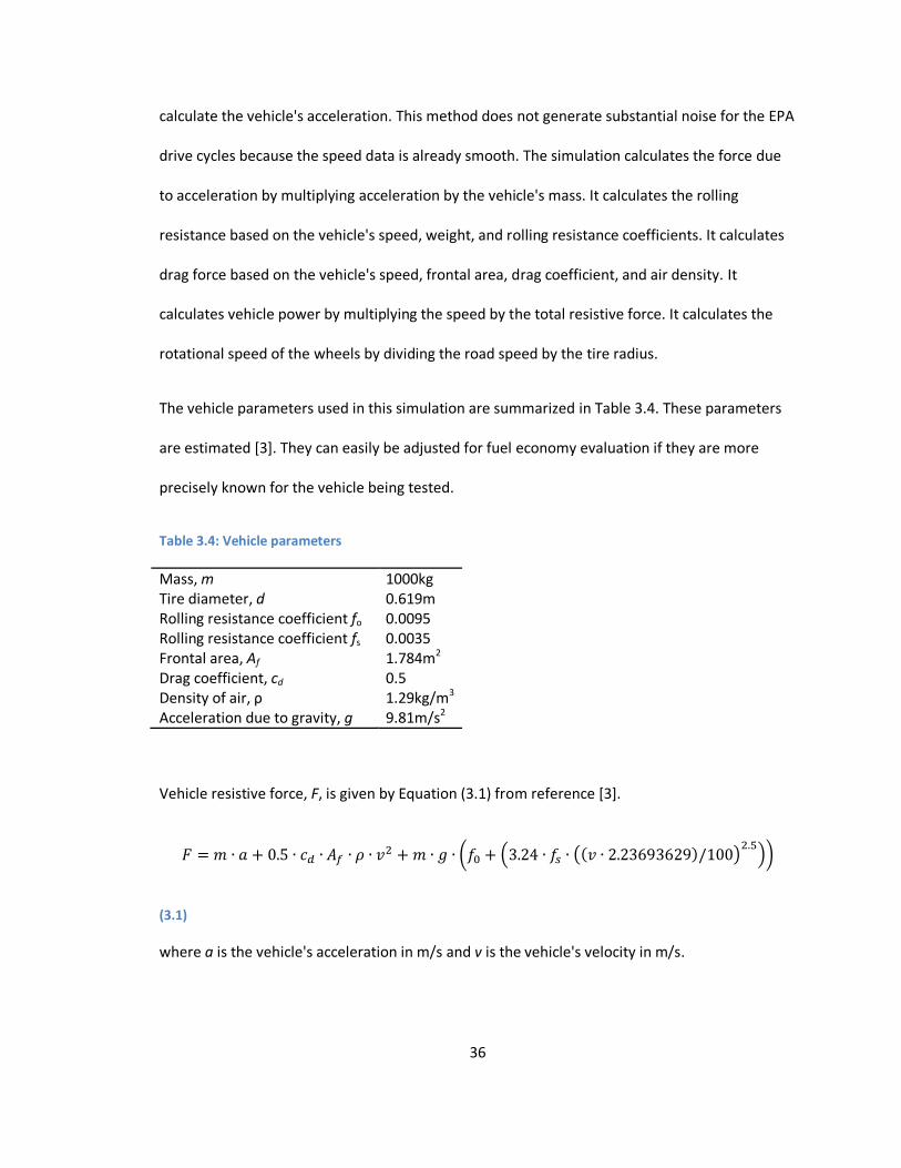
The vehicle parameters used in this simulation are summarized in Table 3.4. These parameters
are estimated [3]. They can easily be adjusted for fuel economy evaluation if they are more
precisely known for the vehicle being tested.
Table 3.4: Vehicle parameters
Mass, m 1000kg Tire diameter, d 0.619m Rolling resistance coefficient fo 0.0095 Rolling resistance coefficient fs 0.0035 Frontal area, Af 1.784m2 Drag coefficient, cd 0.5 Density of air, ρ 1.29kg/m3
Acceleration due to gravity, g 9.81m/s2
Vehicle resistive force, F, is given by Equation (3.1) from reference [3].
(3.1)
where a is the vehicle's acceleration in m/s and v is the vehicle's velocity in m/s.
37
The first term of Equation (3.1) represents the acceleration force on the vehicle. The second
term represents the aerodynamic drag force. The third term represents the tire rolling drag
force.
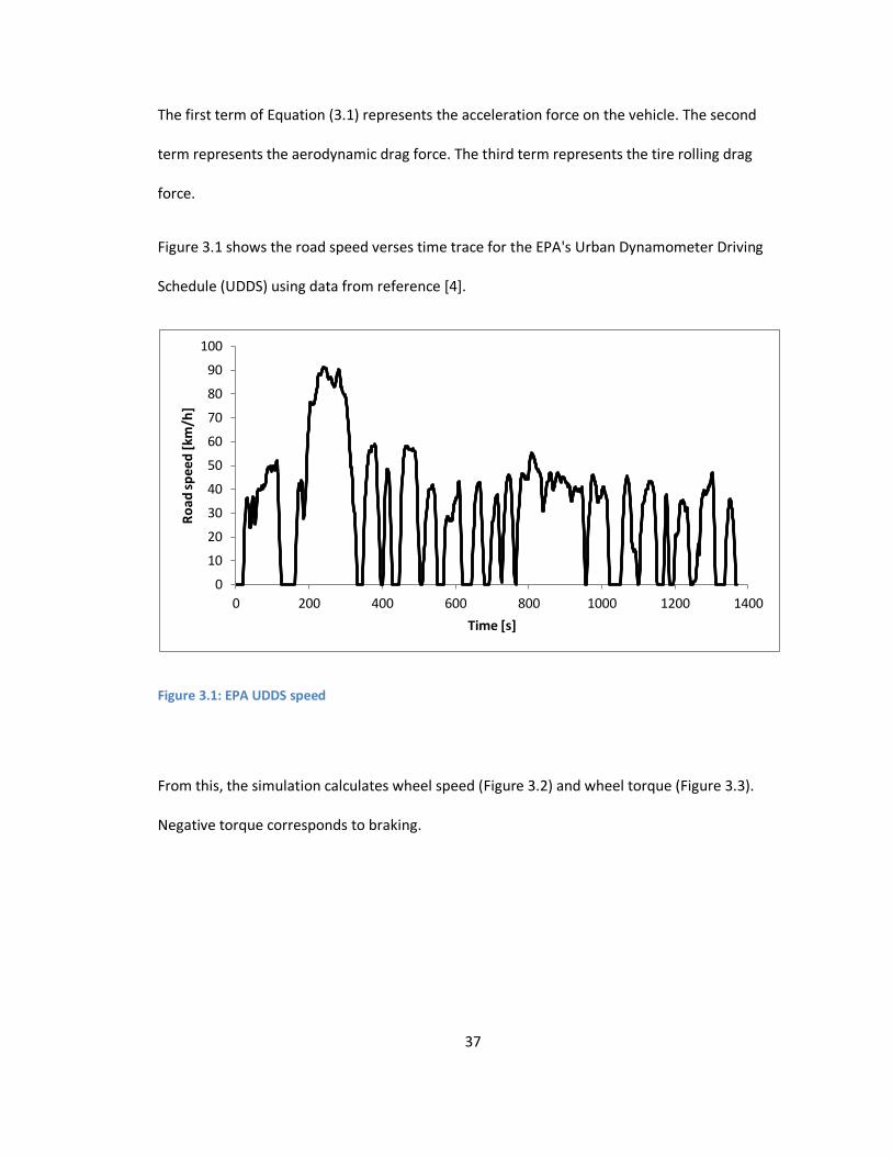
Figure 3.1 shows the road speed verses time trace for the EPA's Urban Dynamometer Driving
Schedule (UDDS) using data from reference [4].
Figure 3.1: EPA UDDS speed
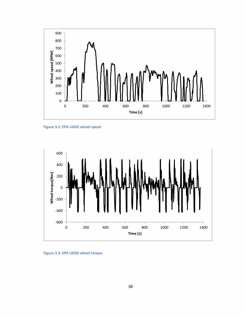
From this, the simulation calculates wheel speed (Figure 3.2) and wheel torque (Figure 3.3).
Negative torque corresponds to braking.
0
10
20
30
40
50
60
70
80
90
100
0 200 400 600 800 1000 1200 1400
Ro
ad s
pee
d [
km/h
]
Time [s]
38
Figure 3.2: EPA UDDS wheel speed
Figure 3.3: EPA UDDS wheel torque
0
100
200
300
400
500
600
700
800
900
0 200 400 600 800 1000 1200 1400
Wh
ee
l sp
ee
d [R
PM
]
Time [s]
-600
-400
-200
0
200
400
600
0 200 400 600 800 1000 1200 1400
Wh
eel t
orq
ue[
Nm
]
Time [s]
39
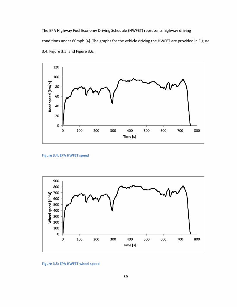
The EPA Highway Fuel Economy Driving Schedule (HWFET) represents highway driving
conditions under 60mph [4]. The graphs for the vehicle driving the HWFET are provided in Figure
3.4, Figure 3.5, and Figure 3.6.
Figure 3.4: EPA HWFET speed
Figure 3.5: EPA HWFET wheel speed
0
20
40
60
80
100
120
0 100 200 300 400 500 600 700 800
Ro
ad s
pe
ed
[km
/h]
Time [s]
0
100
200
300
400
500
600
700
800
900
0 100 200 300 400 500 600 700 800
Wh
eel s
pee
d [R
PM
]
Time [s]
40
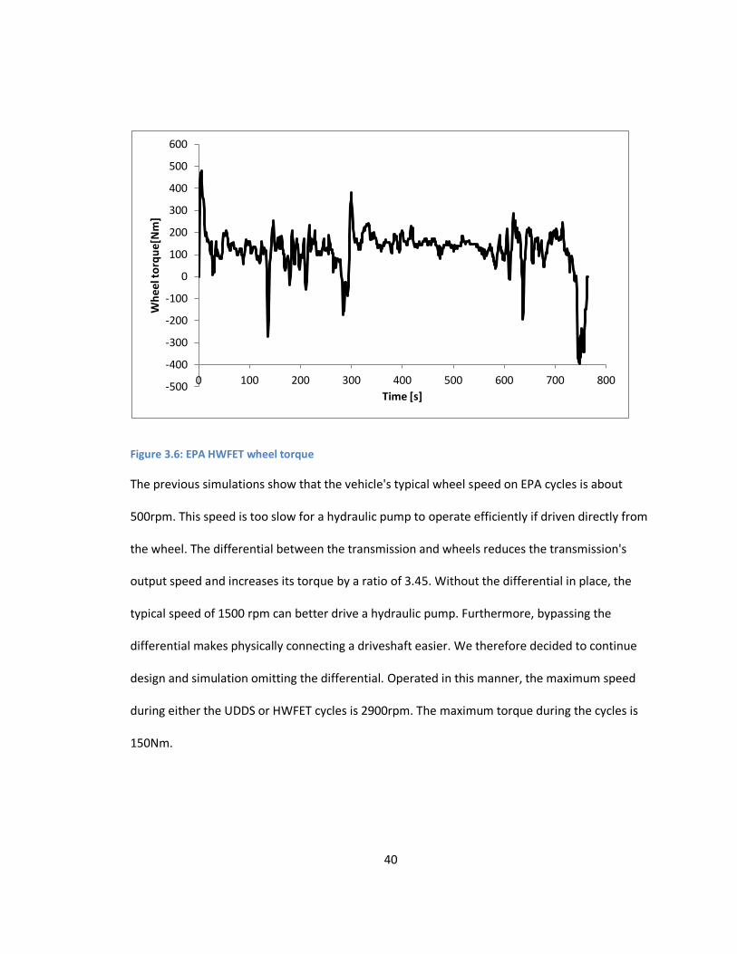
Figure 3.6: EPA HWFET wheel torque
The previous simulations show that the vehicle's typical wheel speed on EPA cycles is about
500rpm. This speed is too slow for a hydraulic pump to operate efficiently if driven directly from
the wheel. The differential between the transmission and wheels reduces the transmission's
output speed and increases its torque by a ratio of 3.45. Without the differential in place, the
typical speed of 1500 rpm can better drive a hydraulic pump. Furthermore, bypassing the
differential makes physically connecting a driveshaft easier. We therefore decided to continue
design and simulation omitting the differential. Operated in this manner, the maximum speed
during either the UDDS or HWFET cycles is 2900rpm. The maximum torque during the cycles is
150Nm.
-500
-400
-300
-200
-100
0
100
200
300
400
500
600
0 100 200 300 400 500 600 700 800
Wh
ee
l to
rqu
e[N
m]
Time [s]
41
3.6 MATLAB simulation of dynamometer
Two simulations were created to model the dynamometer. Each simulation serves a distinct
purpose. The purpose of the simulation created in MATLAB is to validate component sizing. The
purpose of the simulation created in Simulink is to aid the development of the dynamometer's
controller. The MATLAB simulation is described in this section. The Simulink simulation is
described in section 3.7 beginning on page 47.
The MATLAB simulation of the dynamometer following the EPA UDDS and HWFET cycles was
created to size the accumulator, oil cooler, hoses, and valves. The simulation also verified that
existing components could be used as the dynamometer driving pump and power unit. It is
intended to provide only a rough estimate of dynamometer operating parameters; parasitic
losses such as the charge pump and viscous losses are neglected. It is intended to validate the
sizing of a package of components but not to optimize the selection. The code for the simulation
appears in Appendix D. The inputs of the simulation are dynamometer driving pump speed,
torque, and displacement. The simulation outputs are dynamometer driving pump pressure,
flow rate, and accumulator fluid volume.
The simulation assumes that the dynamometer is configured in a manner similar to what is
shown in Figure 2.3 on page 13. However, it assumes that the accumulator's pressure is reduced
by simple throttling for use by the dynamometer driving pump and that this is achieved by some
method which may not be the proportional directional valve. It assumes that the accumulator's
pressure is constant.
The simulation assumes that the output of the vehicle's transmission directly turns the
dynamometer driving pump and that the differential is removed. It calculates hydraulic
42
pressures and flow rates for given vehicle speeds and torques calculated in the separate
MATLAB simulation of the vehicle. The pressure at the dynamometer driving pump necessary to
produce the desired torque is:
(3.2)
where is dynamometer driving pump pressure in bar, is torque in Nm at the dynamometer
driving pump's shaft, and x is the dynamometer driving pump's displacement in cc/rev. The
factor of 10 is necessary because P is in bar and x is in cc/rev. The purpose of Equation (3.2) is to
determine if the pressure required at the dynamometer driving pump to produce the torque
required by the drive cycle is below the maximum system pressure. x is chosen manually and
can vary with time if desired.
The proportional directional valve would be used on the physical dynamometer to regulate the
pressure this way. The flow rate through the dynamometer driving pump is:
(3.3)
where Q is the flow rate in LPM and RPM is the dynamometer driving pump's shaft speed in
RPM. RPM is fixed by the drive cycle. x is again chosen manually. Determining the flow rate
through the dynamometer driving pump with Equation (3.3) is useful for a number of reasons. It
is used to calculate the accumulator's state of charge, which ensures the accumulator will be
large enough to complete motoring events. This flow rate is also necessary to size the valves,
fluid connectors, and oil cooler.
In reality, the dynamometer driving pump's displacement may be varied to control torque, and
the proportional directional valve could be left fully open. In this case, the dynamometer's
43
controller would output a displacement command based on measured and desired torque, and
monitoring pressure would be optional. The current MATLAB simulation is not intended to
model the system operated in this manner since it assumes that the proportional directional
valve's throttling controls the pressure to control the torque. However, it is conservative and
can still validate component sizing conservatively because the dynamometer operates more
efficiently when the proportional directional valve is not throttling.
The sizes of dynamometer components are entered into the simulation prior to execution. If
the component sizes do not produce the desired results, the sizes can be changed and the
simulation rerun.
The most commonly used results of the simulation are the volume of fluid in the accumulator
and pressure at the dynamometer driving pump. The variation of pressure with accumulator
state of charge is neglected. This pressure depends on the accumulator's nitrogen precharge
pressure. If the precharge pressure is high enough to provide enough torque at the
dynamometer driving pump when the accumulator is nearly empty, the system pressure will
remain at least that high as long as oil is in the accumulator.
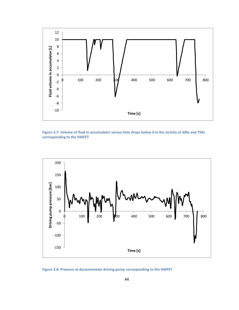
Figure 3.7 shows the volume of fluid in the dynamometer's accumulator during the HWFET with
a constant dynamometer driving pump displacement of 50cc/rev and 10L of fluid initially in the
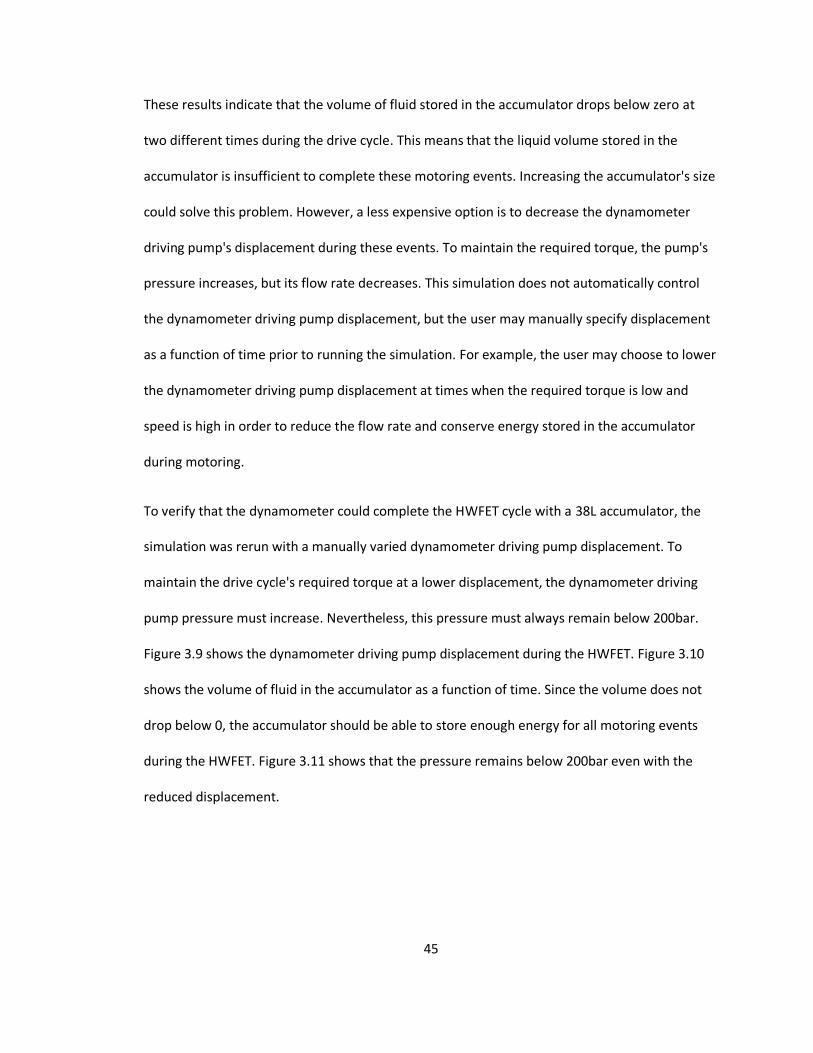
accumulator, a reasonable amount for a 38L accumulator. Figure 3.8 shows the pressure at the
dynamometer driving pump for the same test. Positive pressures correspond to when the
dynamometer is absorbing power; negative pressures correspond to when the dynamometer is
motoring.
44
Figure 3.7: Volume of fluid in accumulator versus time drops below 0 in the vicinity of 300s and 750s corresponding to the HWFET
Figure 3.8: Pressure at dynamometer driving pump corresponding to the HWFET
-10
-8
-6
-4
-2
0
2
4
6
8
10
12
0 100 200 300 400 500 600 700 800
Flu
id v
olu
me
in a
ccu
mu
lato
r [L
]
Time [s]
-150
-100
-50
0
50
100
150
200
0 100 200 300 400 500 600 700 800
Dri
vin
g p
um
p p
ress
ure
[bar
]
Time [s]
45
These results indicate that the volume of fluid stored in the accumulator drops below zero at
two different times during the drive cycle. This means that the liquid volume stored in the
accumulator is insufficient to complete these motoring events. Increasing the accumulator's size
could solve this problem. However, a less expensive option is to decrease the dynamometer
driving pump's displacement during these events. To maintain the required torque, the pump's
pressure increases, but its flow rate decreases. This simulation does not automatically control
the dynamometer driving pump displacement, but the user may manually specify displacement
as a function of time prior to running the simulation. For example, the user may choose to lower
the dynamometer driving pump displacement at times when the required torque is low and
speed is high in order to reduce the flow rate and conserve energy stored in the accumulator
during motoring.
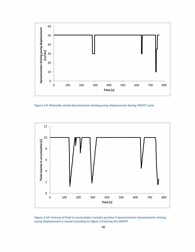
To verify that the dynamometer could complete the HWFET cycle with a 38L accumulator, the
simulation was rerun with a manually varied dynamometer driving pump displacement. To
maintain the drive cycle's required torque at a lower displacement, the dynamometer driving
pump pressure must increase. Nevertheless, this pressure must always remain below 200bar.
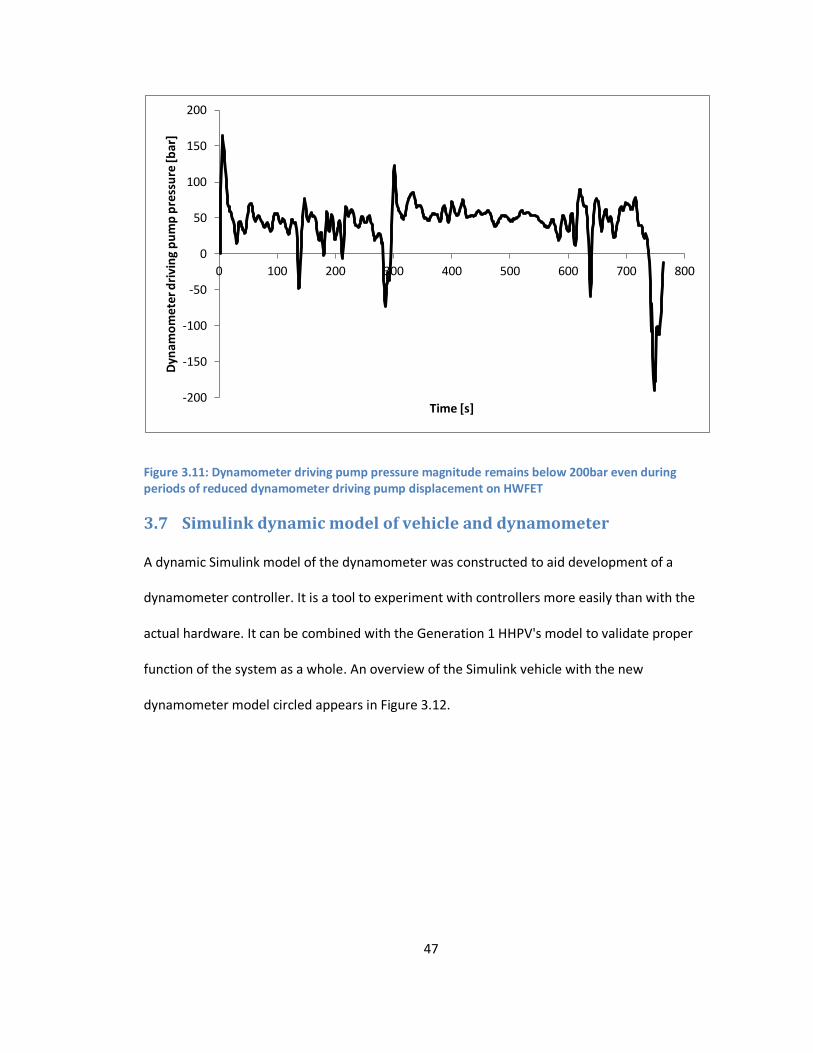
Figure 3.9 shows the dynamometer driving pump displacement during the HWFET. Figure 3.10
shows the volume of fluid in the accumulator as a function of time. Since the volume does not
drop below 0, the accumulator should be able to store enough energy for all motoring events
during the HWFET. Figure 3.11 shows that the pressure remains below 200bar even with the
reduced displacement.
46
Figure 3.9: Manually varied dynamometer driving pump displacement during HWFET cycle
Figure 3.10: Volume of fluid in accumulator remains positive if dynamometer dynamometer driving pump displacement is varied according to Figure 3.9 during the HWFET
0
10
20
30
40
50
60
0 100 200 300 400 500 600 700 800
Dyn
amo
me
ter
dri
vin
g p
um
p d
isp
lace
me
nt
[cc/
rev]
Time [s]
0
2
4
6
8
10
12
0 100 200 300 400 500 600 700 800
Flu
id v
olu
me
in a
ccu
mu
lato
r [L]
Time [s]
47
Figure 3.11: Dynamometer driving pump pressure magnitude remains below 200bar even during periods of reduced dynamometer driving pump displacement on HWFET
3.7 Simulink dynamic model of vehicle and dynamometer
A dynamic Simulink model of the dynamometer was constructed to aid development of a
dynamometer controller. It is a tool to experiment with controllers more easily than with the
actual hardware. It can be combined with the Generation 1 HHPV's model to validate proper
function of the system as a whole. An overview of the Simulink vehicle with the new
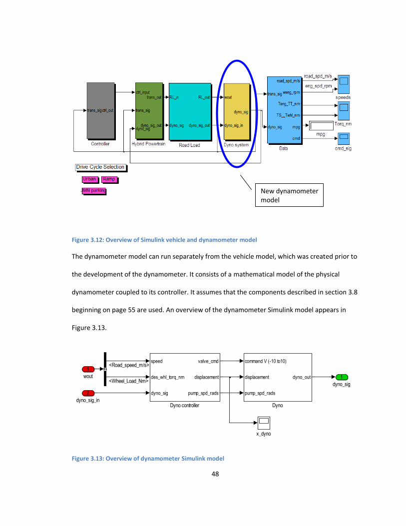
dynamometer model circled appears in Figure 3.12.
-200
-150
-100
-50
0
50
100
150
200
0 100 200 300 400 500 600 700 800
Dyn
amo
me
ter
dri
vin
g p
um
p p
ress
ure
[bar
]
Time [s]
48
Figure 3.12: Overview of Simulink vehicle and dynamometer model
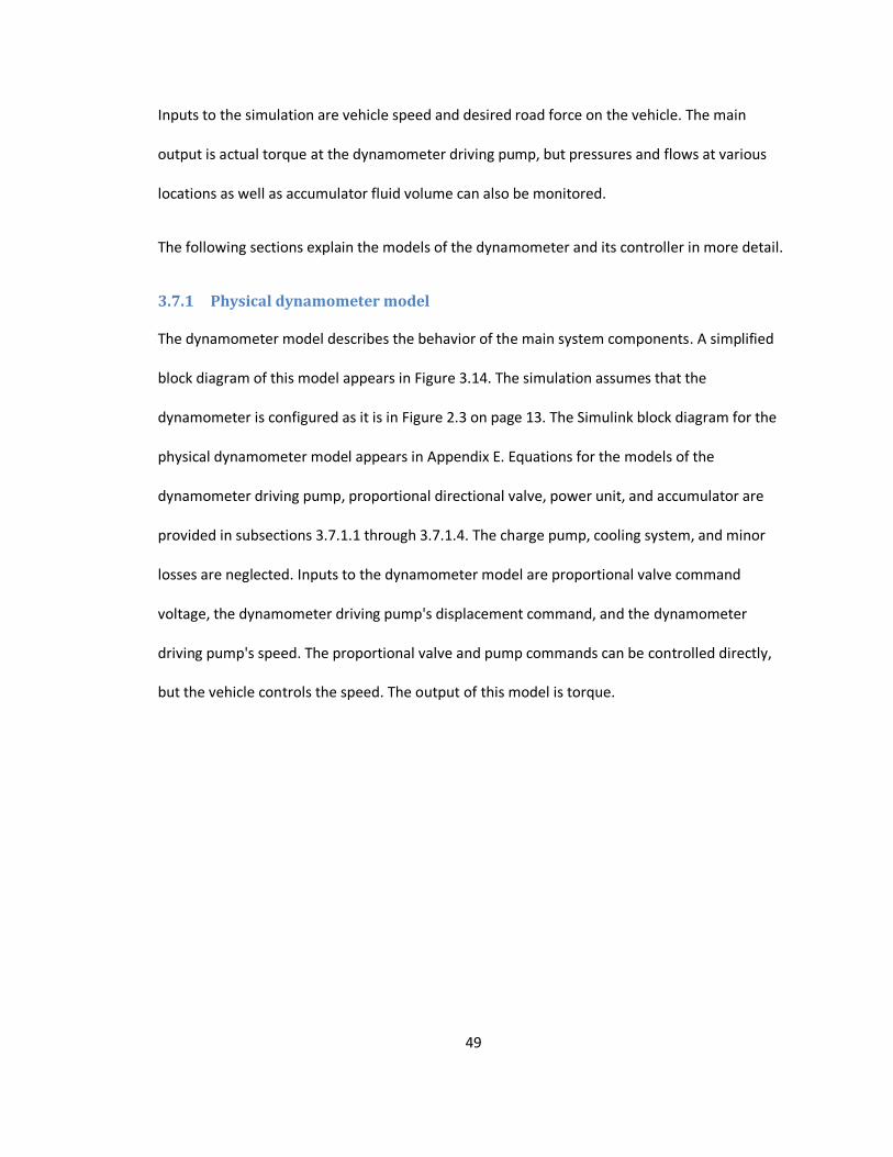
The dynamometer model can run separately from the vehicle model, which was created prior to
the development of the dynamometer. It consists of a mathematical model of the physical
dynamometer coupled to its controller. It assumes that the components described in section 3.8
beginning on page 55 are used. An overview of the dynamometer Simulink model appears in
Figure 3.13.
Figure 3.13: Overview of dynamometer Simulink model
1
dyno_sig
x_dyno
speed
des_whl_torq_nm
dyno_sig
valve_cmd
displacement
pump_spd_rads
Dyno controller
command V (-10 to10)
displacement
pump_spd_rads
dyno_out
Dyno
2
dyno_sig_in
1
wout
<Road_speed_m/s>
<Wheel_Load_Nm>
New dynamometer model
49
Inputs to the simulation are vehicle speed and desired road force on the vehicle. The main
output is actual torque at the dynamometer driving pump, but pressures and flows at various
locations as well as accumulator fluid volume can also be monitored.
The following sections explain the models of the dynamometer and its controller in more detail.
3.7.1 Physical dynamometer model
The dynamometer model describes the behavior of the main system components. A simplified
block diagram of this model appears in Figure 3.14. The simulation assumes that the
dynamometer is configured as it is in Figure 2.3 on page 13. The Simulink block diagram for the
physical dynamometer model appears in Appendix E. Equations for the models of the
dynamometer driving pump, proportional directional valve, power unit, and accumulator are
provided in subsections 3.7.1.1 through 3.7.1.4. The charge pump, cooling system, and minor
losses are neglected. Inputs to the dynamometer model are proportional valve command
voltage, the dynamometer driving pump's displacement command, and the dynamometer
driving pump's speed. The proportional valve and pump commands can be controlled directly,
but the vehicle controls the speed. The output of this model is torque.
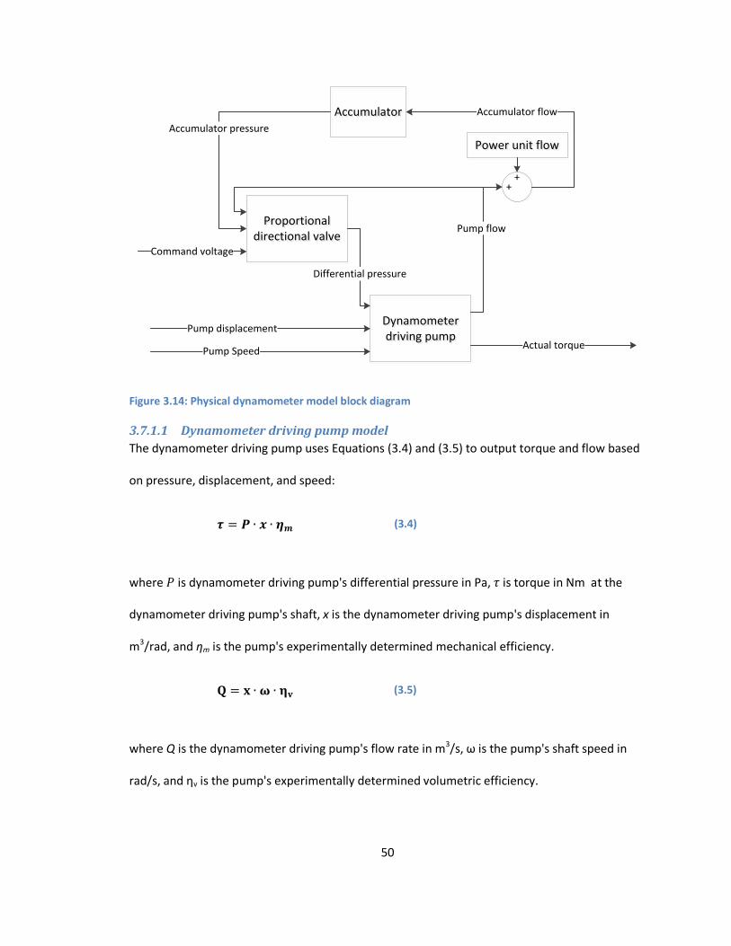
50
++
Dynamometer driving pump
Dynamometer driving pump
Proportional directional valve
Proportional directional valve
Power unit flowPower unit flow
AccumulatorAccumulator
Differential pressure
Pump displacement
Pump Speed
Command voltage
Pump flow
Accumulator flow
Accumulator pressure
Actual torque
Figure 3.14: Physical dynamometer model block diagram
3.7.1.1 Dynamometer driving pump model
The dynamometer driving pump uses Equations (3.4) and (3.5) to output torque and flow based
on pressure, displacement, and speed:
(3.4)
where is dynamometer driving pump's differential pressure in Pa, is torque in Nm at the
dynamometer driving pump's shaft, x is the dynamometer driving pump's displacement in
m3/rad, and ηm is the pump's experimentally determined mechanical efficiency.
(3.5)
where Q is the dynamometer driving pump's flow rate in m3/s, ω is the pump's shaft speed in
rad/s, and ηv is the pump's experimentally determined volumetric efficiency.
51
The dynamometer driving pump was tested extensively in reference [15] to determine ηm and
ηv. Torque, speed, pressure, and flow was measured with the pump on a test stand to
determine ηm and ηv as a function of x, P, and ω.
3.7.1.2 Proportional directional valve model
The model for the proportional directional valve follows the equation for a variable orifice. It
calculates the pressure drop between the high pressure line and one working port as well as the
pressure drop between the tank line and the other working port. The valve's orifice constants
are assumed to be proportional to input voltage. The model calculates pressure drops across the
valve, ΔP, using Equation (3.6)
(3.6)
where V is the command voltage and k is a constant for the valve, estimated based on
observation to be 2·10-7 m3s-1V-1Pa-1/2. The quantity V·k is the orifice constant. Since during
throttling the inlet pressure is assumed to be higher than the outlet pressure, ΔP is positive.
Calculated pressures at the valve's working ports saturate at the maximum system pressure to
simulate a relief valve opening and at 0bar to simulate an anti-cavitation check valve opening.
3.7.1.3 Hydraulic power unit model
The hydraulic power unit is modeled as a source of constant flow, producing 0.00031m3/s
(19LPM).
3.7.1.4 Accumulator model
The accumulator is modeled using the ideal gas law such that its pressure depends on the
volume of liquid contained in it and its precharge pressure. Expansion and compression of the
gas is assumed to be isothermal. The accumulator pressure is given by Equation (3.7).
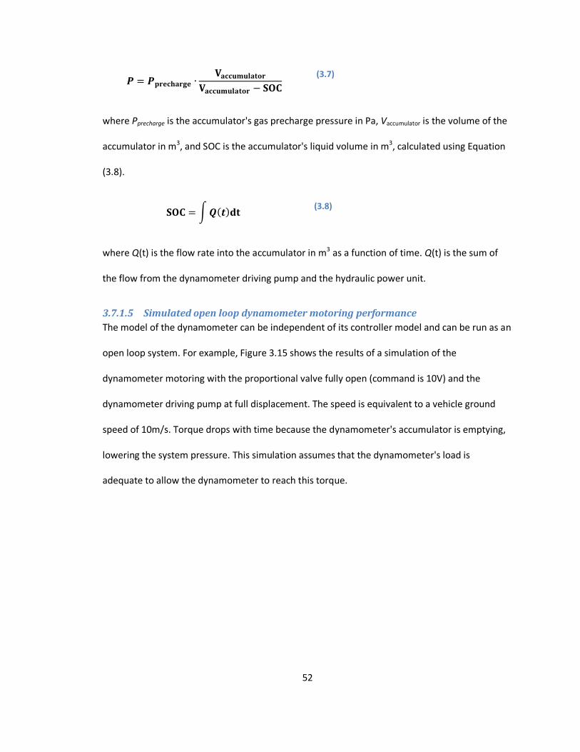
52
(3.7)
where Pprecharge is the accumulator's gas precharge pressure in Pa, Vaccumulator is the volume of the
accumulator in m3, and SOC is the accumulator's liquid volume in m3, calculated using Equation
(3.8).
(3.8)
where Q(t) is the flow rate into the accumulator in m3 as a function of time. Q(t) is the sum of
the flow from the dynamometer driving pump and the hydraulic power unit.
3.7.1.5 Simulated open loop dynamometer motoring performance
The model of the dynamometer can be independent of its controller model and can be run as an
open loop system. For example, Figure 3.15 shows the results of a simulation of the
dynamometer motoring with the proportional valve fully open (command is 10V) and the
dynamometer driving pump at full displacement. The speed is equivalent to a vehicle ground
speed of 10m/s. Torque drops with time because the dynamometer's accumulator is emptying,
lowering the system pressure. This simulation assumes that the dynamometer's load is
adequate to allow the dynamometer to reach this torque.
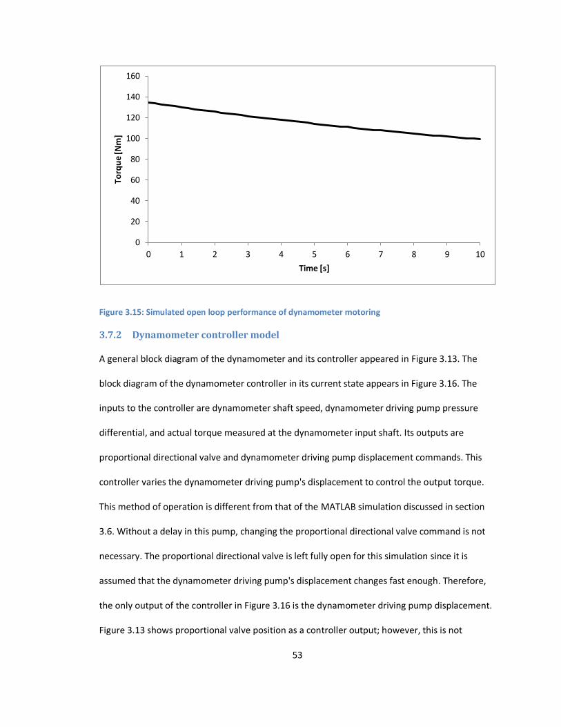
53
Figure 3.15: Simulated open loop performance of dynamometer motoring
3.7.2 Dynamometer controller model
A general block diagram of the dynamometer and its controller appeared in Figure 3.13. The
block diagram of the dynamometer controller in its current state appears in Figure 3.16. The
inputs to the controller are dynamometer shaft speed, dynamometer driving pump pressure
differential, and actual torque measured at the dynamometer input shaft. Its outputs are
proportional directional valve and dynamometer driving pump displacement commands. This
controller varies the dynamometer driving pump's displacement to control the output torque.
This method of operation is different from that of the MATLAB simulation discussed in section
3.6. Without a delay in this pump, changing the proportional directional valve command is not
necessary. The proportional directional valve is left fully open for this simulation since it is
assumed that the dynamometer driving pump's displacement changes fast enough. Therefore,
the only output of the controller in Figure 3.16 is the dynamometer driving pump displacement.
Figure 3.13 shows proportional valve position as a controller output; however, this is not
0
20
40
60
80
100
120
140
160
0 1 2 3 4 5 6 7 8 9 10
Torq
ue
[Nm
]
Time [s]
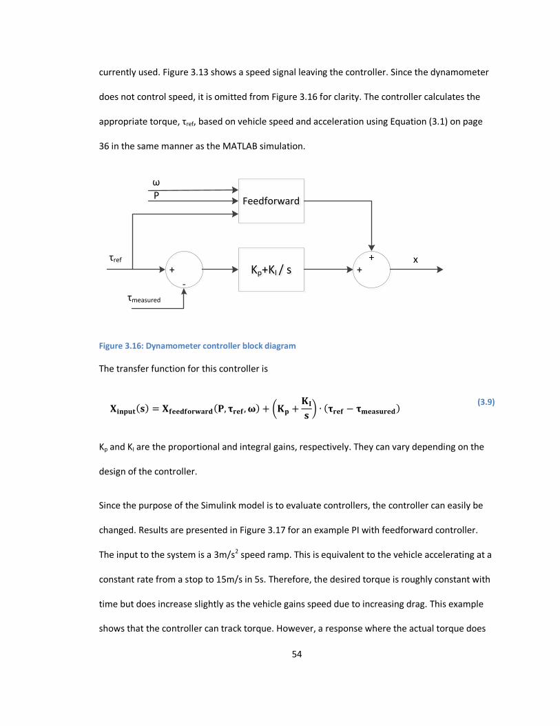
54
currently used. Figure 3.13 shows a speed signal leaving the controller. Since the dynamometer
does not control speed, it is omitted from Figure 3.16 for clarity. The controller calculates the
appropriate torque, τref, based on vehicle speed and acceleration using Equation (3.1) on page
36 in the same manner as the MATLAB simulation.
FeedforwardFeedforward
++
ω P
Kp+KI / sKp+KI / s+
-
τref
τmeasured
x
Figure 3.16: Dynamometer controller block diagram
The transfer function for this controller is
(3.9)
Kp and KI are the proportional and integral gains, respectively. They can vary depending on the
design of the controller.
Since the purpose of the Simulink model is to evaluate controllers, the controller can easily be
changed. Results are presented in Figure 3.17 for an example PI with feedforward controller.
The input to the system is a 3m/s2 speed ramp. This is equivalent to the vehicle accelerating at a
constant rate from a stop to 15m/s in 5s. Therefore, the desired torque is roughly constant with
time but does increase slightly as the vehicle gains speed due to increasing drag. This example
shows that the controller can track torque. However, a response where the actual torque does
55
not overshoot the desired torque would be preferable if it can be achieved without tradeoffs.
The overshoot plateaus between 2s and 2.5 s because this particular simulation saturates the
pump displacement command at 28cc/rev.
Figure 3.17: Imperfect simulated torque tracking using an example controller
3.8 Component selection
Subsections 3.8.1 through 3.8.3, 3.8.5 through 3.8.8, and 3.8.10 describe components reused
from previous projects to reduce cost. The dynamometer driving pump, proportional directional
valve, hydraulic power unit, high pressure filter, data acquisition equipment, cold water supply,
and concrete bed plate were reused. Subsections 3.8.4, 3.8.9, and 3.8.11 describe the selection
of purchased components including the accumulator, oil cooler, and drive shaft.
0
10
20
30
40
50
60
70
80
90
100
0 0.5 1 1.5 2 2.5 3 3.5 4 4.5 5
Torq
ue
[Nm
]
Time [s]
Desired torque (Nm)
Actual torque (Nm)
56
3.8.1 Dynamometer driving pump
Two Sauer-Danfoss Series 42 28cc/rev axial piston pumps were available and selected for use
together as the dynamometer driving pump. Their displacement is infinitely variable from -28 to
28cc/rev. They can be coupled together in a tandem configuration to create a total maximum
displacement of 56cc/rev. This tandem configuration offers no advantage to this application
over a single 56 cc/rev pump and in fact increases the complexity and cost of plumbing and
wiring. These pumps also can only accommodate a charge pump with an uncommon 11 tooth
spline, limiting the selection of charge pumps available with an acceptable lead time. They also
require a low pressure relief valve on the return line to create about 14bar of backpressure so
that their charge flow consumption remains low. We do not understand why the backpressure is
necessary.
A larger 100cc/rev pump was available but not selected for use because its displacement was
too large for the application. It would have to be operated in an inefficient low displacement
regime, limiting the power available for motoring. This pump could be used later if testing a
more powerful vehicle is necessary.
3.8.2 Proportional directional valve
An Eaton KFDG5V-7 two stage proportional directional valve was available and selected to
provide a faster alternative to control load than by changing the pump displacement. Although
its specifications meet or exceed requirements of the application, the valve required substantial
effort to become usable. The valve is two stage and pilot operated. The pilot stage is a solenoid
operated directional valve that provides pilot pressure to move the main stage spool. It requires
a sandwich reducing valve to be installed between the main stage and the pilot stage to reduce
57
pressure for the pilot stage [12, p. 2]. This was purchased and installed. We also needed to
purchase the proper amplifier, connectors, and wiring.
Although it is common to use a proportional directional valve to control a motor's speed, using
one to control a pump's speed is uncommon. A proportional relief valve was considered for load
control during absorbing (pumping). This valve would replace the proportional directional valve
to control the outlet pressure of the pump directly. However, we decided to use only the
existing proportional directional valve to avoid the cost of purchasing a new valve. Verification
of the proportional directional valve's ability to control load of a pump was therefore necessary.
To verify the valve's ability to control a pump's speed, the circuit shown in Figure 3.18 was built.
The shaft of a fixed displacement pump was coupled to the shaft of a fixed displacement motor.
Torque and speed were measured at this connection. Since the motor was connected to a
constant pressure source, it provided a constant torque. The pump was connected to the valve.
The pump's displacement was kept high enough to prevent over pressurization, however, using
a relief valve in addition would have been safer.
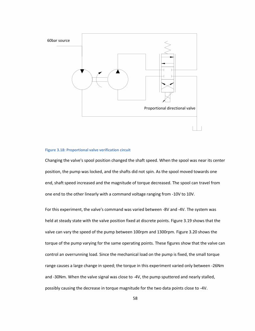
58
60bar source
Proportional directional valve
Figure 3.18: Proportional valve verification circuit
Changing the valve's spool position changed the shaft speed. When the spool was near its center
position, the pump was locked, and the shafts did not spin. As the spool moved towards one
end, shaft speed increased and the magnitude of torque decreased. The spool can travel from
one end to the other linearly with a command voltage ranging from -10V to 10V.
For this experiment, the valve's command was varied between -8V and -4V. The system was
held at steady state with the valve position fixed at discrete points. Figure 3.19 shows that the
valve can vary the speed of the pump between 100rpm and 1300rpm. Figure 3.20 shows the
torque of the pump varying for the same operating points. These figures show that the valve can
control an overrunning load. Since the mechanical load on the pump is fixed, the small torque
range causes a large change in speed; the torque in this experiment varied only between -26Nm
and -30Nm. When the valve signal was close to -4V, the pump sputtered and nearly stalled,
possibly causing the decrease in torque magnitude for the two data points close to -4V.
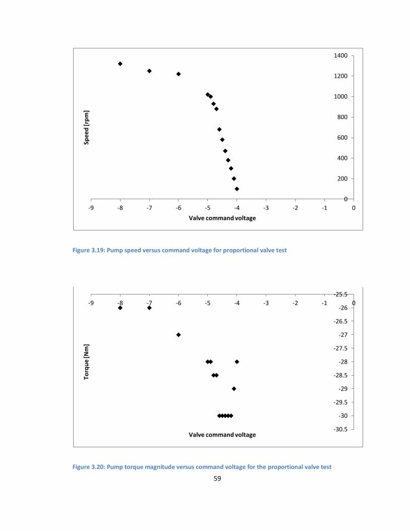
59
Figure 3.19: Pump speed versus command voltage for proportional valve test
Figure 3.20: Pump torque magnitude versus command voltage for the proportional valve test
0
200
400
600
800
1000
1200
1400
-9 -8 -7 -6 -5 -4 -3 -2 -1 0
Spe
ed
[rp
m]
Valve command voltage
-30.5
-30
-29.5
-29
-28.5
-28
-27.5
-27
-26.5
-26
-25.5
-9 -8 -7 -6 -5 -4 -3 -2 -1 0
Torq
ue
[Nm
]
Valve command voltage
60
3.8.3 Hydraulic power unit
The dynamometer's driving pump requires up to 150LPM when motoring at full displacement
during the maximum speed of the EPA drive cycles. The actual flow requirement may be less if
the dynamometer driving pump's displacement is reduced. The power unit is only capable of
producing 19LPM, so an accumulator was necessary to supplement flow.
The power unit contained a relief valve and filter, but they were unable to accommodate the
maximum flow rates of 150LPM and fluid cleanliness requirements of the system, which require
a 3 micron or finer filter element. The existing filter was replaced with one with a larger capacity
and a finer 3 micron element. The relief valve was duplicated with one designed for a higher
flow rate.
Cavitation of the suction line was a concern since the tank could not be raised or pressurized.
This required the use of large hose and valves on the suction line. The power unit's tank did not
previously have a suction line and required one to be installed. Suction flow was necessary for
the charge pump and anti-cavitation check valves.
The maximum pressure of the power unit is 200bar, setting a ceiling for the system. This limit is
practical for other components and did not affect the overall design of the system.
3.8.4 Accumulator
Bladder and piston style accumulators are available. The bladder style was selected due to its
lower cost and lower seal friction. The MATLAB simulation in section 3.6 indicated that a 38L
accumulator should provide adequate energy storage capacity for the dynamometer to
complete the EPA's UDDS and HWFET cycles. A Parker BA10B3T01-A1 accumulator was
ultimately selected.
61
3.8.5 Torque and speed sensor
A Honeywell 1105H-101 slip ring torque sensor was available from a previous pump test stand
project. It also contains a speed sensor module. This sensor can easily measure the full torque
and speed required by the project. It requires regular maintenance according to reference [16].
In particular, the slip ring assembly should be cleaned if the torque signal is noisy, and the
brushes should be replaced once they have worn to less than 8mm in length.
Software to interface with this sensor was already made in Simulink with xPC Target. This
system is described in reference [15, p. 25]. Changing to a different DAQ system would have
required substantial effort to remake this interface software.
3.8.6 Data acquisition equipment
The existing pump test stand used two office style desktop PCs to run xPC Target for controls
and data acquisition. This setup is unreliable; communication between host and target PCs often
drops, and the DAQ cards are easily damaged. Hardware designed for laboratory use would be
preferable, as would a system requiring only a single computer. However, the cost and time
required to integrate a new computer system was prohibitive, so the existing system was used.
3.8.7 Cold water supply
A chilled water supply was not available in the room housing the dynamometer. Therefore, the
existing cold water supply for the sink needed to be used. The oil cooler needed to be sized to
use no more than the flow available from this sink, about 10LPM.
3.8.8 High pressure filter
Instructions for the proportional valve recommend using a 3 micron or finer filter on the high
pressure line upstream of the proportional valve. A high pressure filter was available, but its
62
micron rating of 5 did not meet this specification. Replacing this filter with a new high pressure
filter was too expensive, so it was instead supplemented with an inexpensive 3 micron return
line filter.
3.8.9 Oil cooler
The MATLAB simulation indicated that the dynamometer would absorb 10-15kW of power from
the vehicle that would need to be dissipated in the form of heat. The return oil flow rate would
be 50LPM on average and could reach a maximum of 150LPM. The temperature of the hydraulic
oil should not exceed 70°C. The flow rate of cool water available from the sink is about 10LPM at
10°C.
A Thermasys EK series shell and tube oil cooler was selected because of its low cost and
common availability. The limited flow rate of cool water required an oil cooler sized for at least a
5:1 oil to water ratio. Using instructions in the manufacturer's catalog [17], the power removed
in the cooler was calculated to be 7kW (9hp), and the oil flow was calculated to be 50LPM
(13GPM). Any line above this point on the graph titled "7:1 Oil to Water Ratio – Lower Water
Usage" on page 78 of reference [17] corresponds to an oil cooler that will work. The line
corresponding to model EKS-714-F was selected to be slightly oversized for this application.
Although the dynamometer is capable of absorbing more than 7kW for short times, the oil
cooler only needs to remove the average power.
3.8.10 Concrete bed plate
The concrete bed plate provides a stable, heavy surface for mounting components. All
components with the exception of the power unit must fit on the existing bed plate's 1.9 by
1.2m surface. Drilling new holes into the concrete material is difficult, so moving or remounting
components once they are installed is difficult.
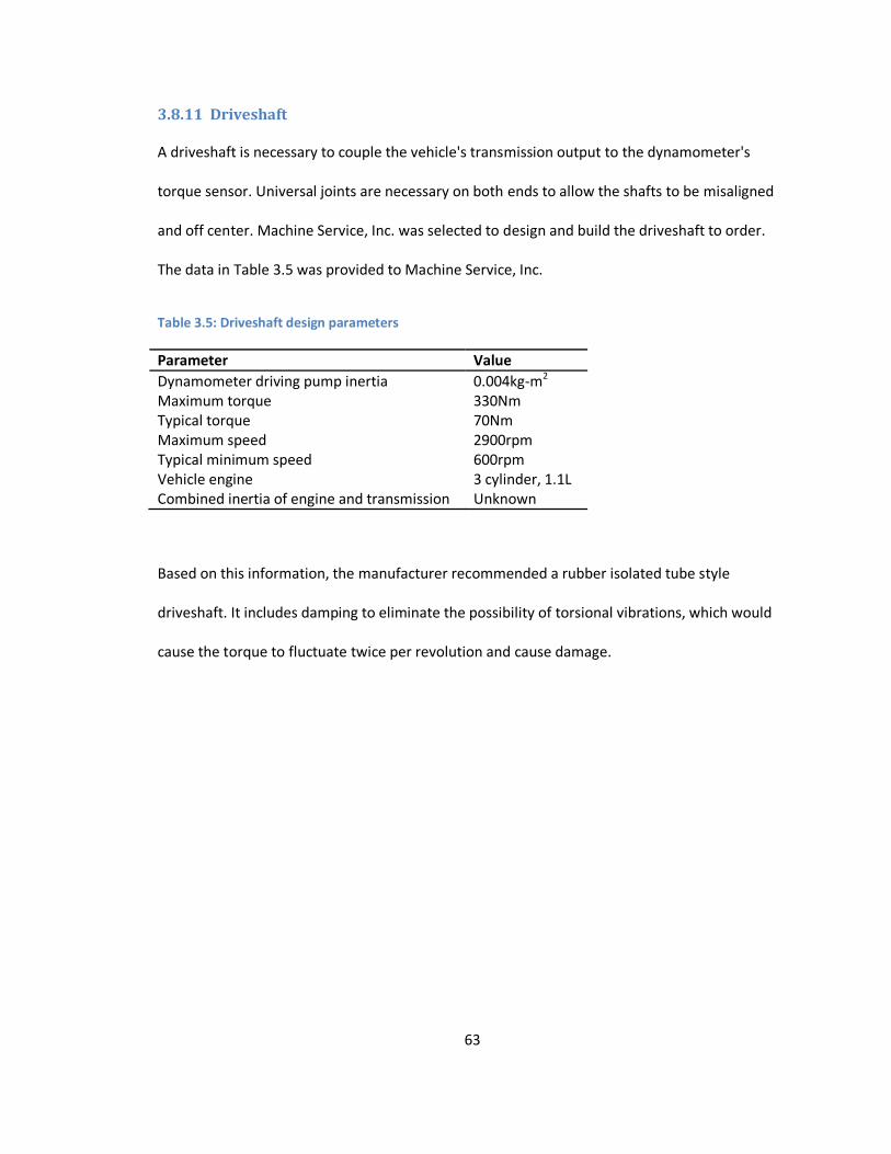
63
3.8.11 Driveshaft
A driveshaft is necessary to couple the vehicle's transmission output to the dynamometer's
torque sensor. Universal joints are necessary on both ends to allow the shafts to be misaligned
and off center. Machine Service, Inc. was selected to design and build the driveshaft to order.
The data in Table 3.5 was provided to Machine Service, Inc.
Table 3.5: Driveshaft design parameters
Parameter Value
Dynamometer driving pump inertia 0.004kg-m2
Maximum torque 330Nm Typical torque 70Nm Maximum speed 2900rpm Typical minimum speed 600rpm Vehicle engine 3 cylinder, 1.1L Combined inertia of engine and transmission Unknown
Based on this information, the manufacturer recommended a rubber isolated tube style
driveshaft. It includes damping to eliminate the possibility of torsional vibrations, which would
cause the torque to fluctuate twice per revolution and cause damage.
64
4 Results and performance of dynamometer
Section 4.1 describes limitations of testing the dynamometer due to vehicle reliability issues.
Section 4.2 describes a test in which the dynamometer motored with open loop control. Section
4.3 describes the process used to determine the dynamometer's transfer function
experimentally and how it will be used for the automatic torque controller. The torque
controller varies the dynamometer driving pump's displacement to produce the desired torque.
Section 4.4 describes the performance of the automatic torque controller. Section 4.5 describes
results from a test when the dynamometer absorbed power from the vehicle. Section 4.6
evaluates the automatic torque controller. Section 4.7 describes the practical environmental,
usability, and reliability aspects of operating the dynamometer.
4.1 Vehicle reliability limited testing
Poor reliability of the Generation 1 HHPV hindered full evaluation of the dynamometer
operating on a drive cycle with the vehicle. The connection between the vehicle's engine and
transmission was particularly unreliable and prevented substantial testing with the vehicle
powering the dynamometer and the dynamometer absorbing power. Evaluation of torque
tracking in response to vehicle speed changes, measuring the dynamometer's maximum torque
and speed, measuring maximum motoring duration, and tracking of an EPA cycle was desired
but not possible. Testing by motoring the vehicle using the dynamometer was possible. The
dynamometer could be coupled to the transmission with the vehicle's engine disconnected from
its transmission. These tests could provide data on the motoring performance of the
dynamometer as well as the energy recovery capabilities of the vehicle's hydraulic system.
65
4.2 Dynamometer open loop control demonstrates motoring torque of
85Nm
For this test, the dynamometer motored the transmission of the vehicle. The vehicle's engine
was disconnected from its transmission, and its pumps were stroked to full displacement in
order to provide a resistance to the dynamometer. The torque and speed of the dynamometer
are shown in Figure 4.1 for a portion of this test. At about 805s into the test, the dynamometer
driving pump displacement was manually increased from 0.4 to 1.0 for the remainder of the
time shown in the plot. This caused its motoring torque to increase from 30Nm to 85Nm which
accelerated the transmission from 1100rpm to 2400rpm. Near this time, the motoring power
peaked at 17kW. As the dynamometer's accumulator emptied, the torque dropped. The
increase of torque beginning near 807s may be a result of a changing load on the vehicle or the
changing efficiency of the dynamometer driving pump.
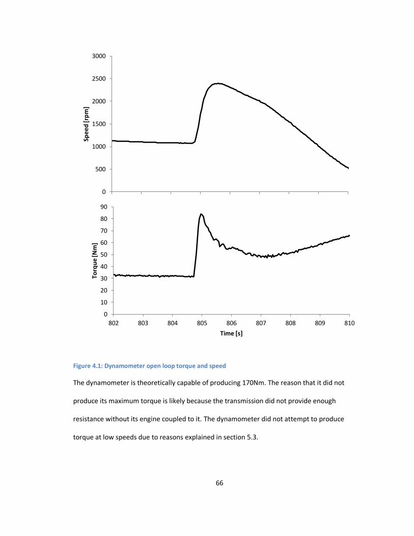
66
Figure 4.1: Dynamometer open loop torque and speed
The dynamometer is theoretically capable of producing 170Nm. The reason that it did not
produce its maximum torque is likely because the transmission did not provide enough
resistance without its engine coupled to it. The dynamometer did not attempt to produce
torque at low speeds due to reasons explained in section 5.3.
0
500
1000
1500
2000
2500
3000
Spe
ed
[rp
m]
0
10
20
30
40
50
60
70
80
90
802 803 804 805 806 807 808 809 810
Torq
ue
[Nm
]
Time [s]
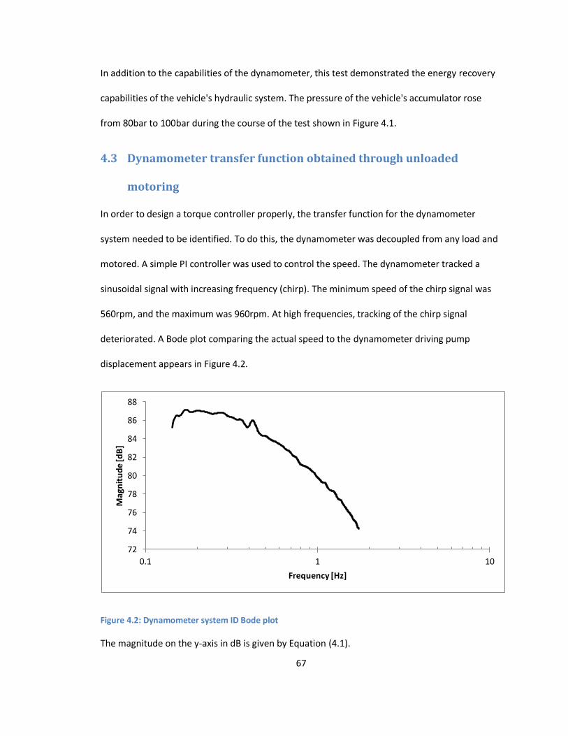
67
In addition to the capabilities of the dynamometer, this test demonstrated the energy recovery
capabilities of the vehicle's hydraulic system. The pressure of the vehicle's accumulator rose
from 80bar to 100bar during the course of the test shown in Figure 4.1.
4.3 Dynamometer transfer function obtained through unloaded
motoring
In order to design a torque controller properly, the transfer function for the dynamometer
system needed to be identified. To do this, the dynamometer was decoupled from any load and
motored. A simple PI controller was used to control the speed. The dynamometer tracked a
sinusoidal signal with increasing frequency (chirp). The minimum speed of the chirp signal was
560rpm, and the maximum was 960rpm. At high frequencies, tracking of the chirp signal
deteriorated. A Bode plot comparing the actual speed to the dynamometer driving pump
displacement appears in Figure 4.2.
Figure 4.2: Dynamometer system ID Bode plot
The magnitude on the y-axis in dB is given by Equation (4.1).
72
74
76
78
80
82
84
86
88
0.1 1 10
Mag
nit
ud
e [d
B]
Frequency [Hz]
68
(4.1)
where RPM is the magnitude of the dynamometer driving pump's shaft speed in RPM and x is
the magnitude of the dynamometer driving pump's displacement scaled to a range of -1 to 1.
This equation was not evaluated at displacements near 0 because the dynamometer driving
pump could not produce enough torque to spin.
The Bode plot was used to determine the transfer function of the dynamometer with driving
pump displacement (on a scale of 0 to 1) as an input and speed (in rpm) as an output. The
transfer function appears as Equation (4.2).
(4.2)
This transfer function is valid for pressures around 180bar. Although it is a transfer function for
speed, it is useful for the torque controller as well because the dynamometer driving pump's
swashplate dynamics are the same regardless of whether speed or torque is being controlled.
4.4 Dynamometer closed loop automatic torque control
Using the transfer function from section 4.3, a torque controller was developed for the
dynamometer. For this experiment, the operator entered a desired torque manually into the
computer. The torque controller operated by the Simulink program coupled to the xPC Target
real time control system adjusted the dynamometer driving pump displacement so that the
actual and desired torque match. For later experiments, the desired torque could be calculated
automatically as a function of speed and the vehicle parameters outlined in section 3.5
beginning on page 35.
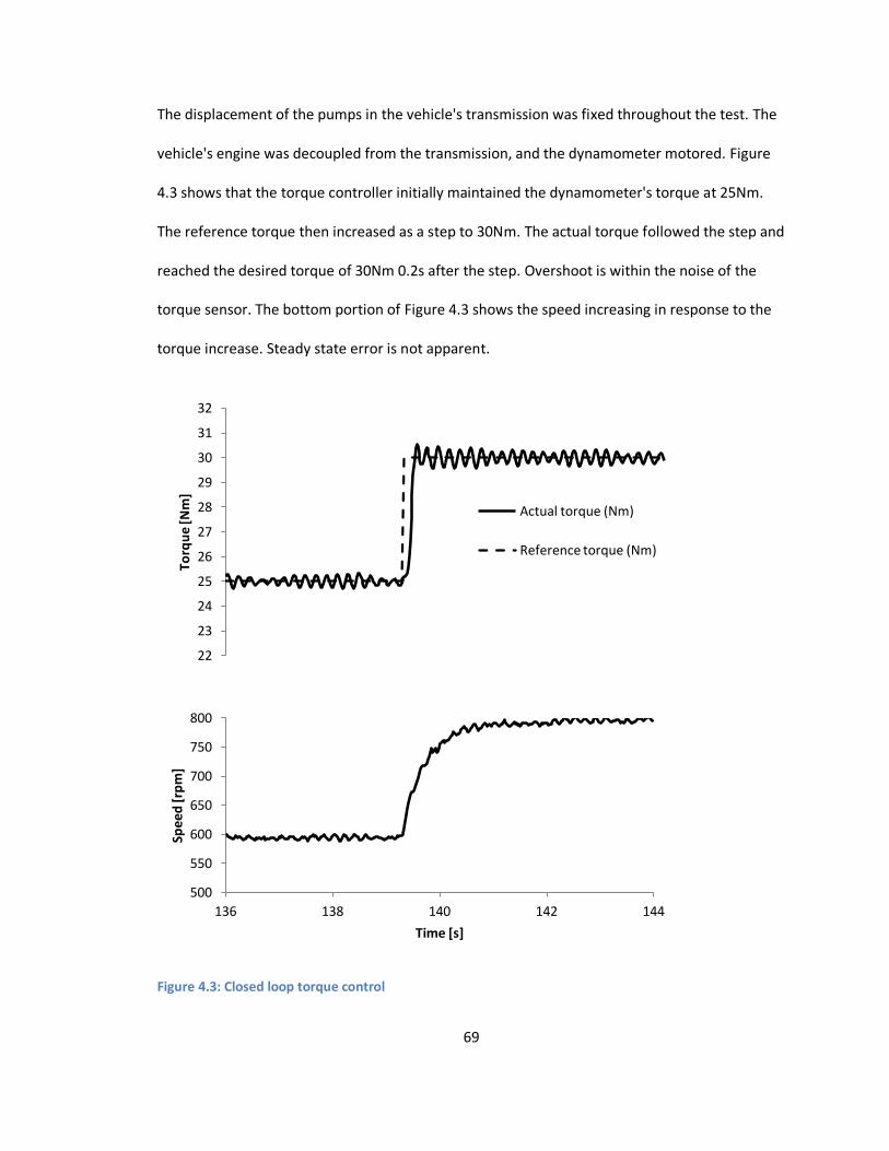
69
The displacement of the pumps in the vehicle's transmission was fixed throughout the test. The
vehicle's engine was decoupled from the transmission, and the dynamometer motored. Figure
4.3 shows that the torque controller initially maintained the dynamometer's torque at 25Nm.
The reference torque then increased as a step to 30Nm. The actual torque followed the step and
reached the desired torque of 30Nm 0.2s after the step. Overshoot is within the noise of the
torque sensor. The bottom portion of Figure 4.3 shows the speed increasing in response to the
torque increase. Steady state error is not apparent.
Figure 4.3: Closed loop torque control
22
23
24
25
26
27
28
29
30
31
32
Torq
ue
[Nm
]
Actual torque (Nm)
Reference torque (Nm)
500
550
600
650
700
750
800
136 138 140 142 144
Spee
d [r
pm
]
Time [s]
70
4.5 Absorbing performance
The dynamometer was able to demonstrate absorbing power from the vehicle for a brief period
of time before a freewheeling clutch between the vehicle's engine and its transmission failed.
The dynamometer driving pump displacement was controlled manually. The vehicle's engine
speed and pump displacements were set manually. Results from a portion of this test appear in
Figure 4.4. Negative torque corresponds to the dynamometer absorbing power. The torque
absorbed by the dynamometer peaked at -42Nm. The speed at that time was 900rpm,
corresponding to 4kW of absorption. The dynamometer is designed to be capable of absorbing
more power and torque; the vehicle was the limiting factor for this test. Since both machines
could change the torque and speed, there is no direct indication of which one is responsible for
the changes in torque and speed observed in Figure 4.4. For example, either an increase in
vehicle throttle or dynamometer driving pump displacement could cause an increase in torque
magnitude.
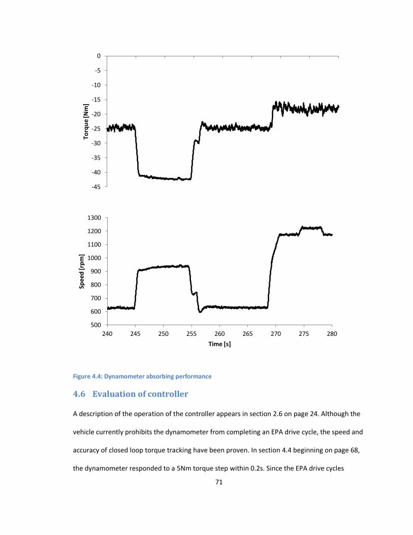
71
Figure 4.4: Dynamometer absorbing performance
4.6 Evaluation of controller
A description of the operation of the controller appears in section 2.6 on page 24. Although the
vehicle currently prohibits the dynamometer from completing an EPA drive cycle, the speed and
accuracy of closed loop torque tracking have been proven. In section 4.4 beginning on page 68,
the dynamometer responded to a 5Nm torque step within 0.2s. Since the EPA drive cycles
-45
-40
-35
-30
-25
-20
-15
-10
-5
0
Torq
ue
[Nm
]
500
600
700
800
900
1000
1100
1200
1300
240 245 250 255 260 265 270 275 280
Spee
d [r
pm
]
Time [s]
72
provide speed data points every 1s, this response time is likely to be fast enough to track the
drive cycles without using the dynamometer's proportional directional valve to improve the
dynamic response of torque tracking. The controller does not currently use the proportional
directional valve.
The selection of hardware contributes to the controller's fast performance. The inertia of a
hydrostatic dynamometer is low compared to other styles of dynamometers. Low inertia allows
the dynamometer to change speeds quickly. Furthermore, the dynamometer driving pump has
the fastest displacement control solenoid available from its manufacturer for this series of
pumps.
4.7 Usability and environmental assessment
The dynamometer generally meets the usability, safety, and environmental requirements set
prior to the start of this project. It has proven to be easy enough to learn how to use that a
graduate student already familiar with MATLAB became a proficient operator within a day.
The dynamometer has begun to show that it is reliable and requires little maintenance. In about
four months of operation it has had only one day of unscheduled downtime due to a blown fuse
in its hydraulic power unit. After the control box was disconnected and reconnected, the
hydraulic power unit started unexpectedly. The fuse blew in the process of troubleshooting the
unexpected startup. The reason for the unexpected startup is not fully understood but seems to
depend on the order in which the controls are connected. Since the rest of the dynamometer's
hydraulic system was shut off, it did not build pressure. Scheduled maintenance has included
replacement of the low pressure filter element.
73
A larger room would improve the operator's ability to move about, make repairs on site, and
move the vehicle in and out. The current space available is 5 by 6m; double that area would be
preferable. Cord drops from the ceiling would be preferable to running wires across the floor to
eliminate tripping risks. The ventilation system is adequate to remove the exhaust from the
vehicle. Noise is a concern as the test is audible from a neighboring office. However, most of the
noise comes from the vehicle rather than the dynamometer. The dynamometer has no
unintentional leaks, but the vehicle does leak gear oil from its transmission and requires a drip
pan underneath.
74
5 Conclusion
This chapter summarizes the accomplishments of this project and the importance of this work. It
also includes recommendations to improve and expand the capabilities of the dynamometer.
5.1 Review
Chapter 1 introduced the vehicle that the dynamometer is designed to test. It listed the
requirements and goals for the project. The EPA test procedure was summarized along with
other dynamometer projects with similar objectives.
Chapter 2 provided a detailed description of the dynamometer and described its hardware
implementation and how it works. A hydraulic schematic of the dynamometer was presented,
and each component was explained. The physical configuration of the machine was described.
Manual and automatic methods of controlling the dynamometer were described. Finally, safety
features and ergonomics were explained.
Chapter 3 described the design process followed to converge on the final product. Using
contract testing services or commercially available dynamometers was considered and
ultimately rejected. A purpose built hydrostatic dynamometer was selected after comparing
three styles of dynamometers. General component specifications were developed using a
MATLAB simulation, and a dynamic model was created in Simulink. Reuse of existing
components to reduce cost imposed design constraints.
Chapter 4 provided experimental results to evaluate the performance of the dynamometer. The
dynamometer torque controller was developed with the dynamometer disconnected from the
vehicle. Some testing and verification was performed with the dynamometer and vehicle
connected.
75
5.2 Contributions
The primary accomplishment of this thesis work is the construction of a hydrostatic
dynamometer to test the Generation 1 HHPV. A special feature of this machine is its ability to
motor as well as absorb power from the vehicle. Experimentally measured power, torque,
speed, and response times indicate that the dynamometer will likely be able to complete EPA
drive cycles when coupled to the Generation 1 HHPV. This dynamometer will validate the fuel
economy of the vehicle. The dynamometer will also allow convenient and repeatable retesting
which is necessary for the comparison and refinement of controls algorithms. This will allow
several students to include experimental results in their theses.
The success of this dynamometer also demonstrates the feasibility of using hydraulics for
dynamometers in general. Hydraulics offer the opportunity to reduce dynamometer cost and
improve dynamic performance. Since many components were reused for this dynamometer, its
cost of parts was low. Manufacturing hydrostatic dynamometers on a larger scale would reduce
the high labor costs. Although all components would need to be purchased for a mass
manufactured hydrostatic dynamometer, in many cases, simpler inexpensive components could
be used.
5.3 Future work
The source of charge pressure for the dynamometer driving pump is a fixed displacement charge
pump directly connected to the shaft. The dynamometer cannot produce torque at low speeds
below about 100rpm because the charge pump spins too slowly to produce enough flow to
maintain charge pressure. This behavior is a byproduct of a safety feature designed to prevent
the dynamometer from turning backwards. If the possibility of the dynamometer turning
backwards is acceptable, a reducing valve could be added to reduce the high pressure to
76
maintain charge pressure at all times. However, this method is inefficient and would diminish
the power available for motoring.
Shortcomings of the Generation 1 HHPV's reliability have prevented full validation of the
capabilities of the dynamometer. Vehicle reliability and durability must improve to enable full
dynamometer performance data to be gained. Reliability of the connection between the
vehicle's engine and transmission has been particularly poor; without this connection, the
absorbing capabilities of the dynamometer could not be thoroughly tested. In addition, the shaft
connection to the sun gear of the planetary gear train utilized within the transmission of the
vehicle began slipping once during testing. The transmission needed to be disassembled to
correct the slipping shaft. If it slips again, the design should be modified.
Once the Generation 1 HHPV is running reliably, the dynamometer's software may need to be
tuned to improve drive cycle tracking and accuracy. Refining the torque controller based on
observations of performance will allow better tracking of the EPA drive cycles. The coefficients
in Table 3.4 on page 36 used to calculate road load in Equation (3.1) on page 36 are estimates
and should be verified before fuel economy data for this particular vehicle is published. The
coefficients can be determined experimentally based on the deceleration of the vehicle coasting
on a test track. However, different coefficients could be entered into the dynamometer to
simulate the Generation 1 HHPV's powertrain in a different vehicle.
The proportional directional valve shown in Figure 2.3 on page 13 is not currently used because
the dynamometer driving pump's displacement control appears to be fast enough. However, if
faster dynamics are desired, controls for this valve will need to be developed.
77
5.4 Possibility of testing other machines
The dynamometer is not limited to testing only the Generation 1 HHPV. It could test another
machine or vehicle with approximately the same power. Prime movers such as motors or
engines could be tested. At maximum torque and speed, it could theoretically absorb 50kW for
short periods. Typical sustained operation could be around 15kW as long as oil temperature is
monitored carefully. Sustained low speed operation below 500rpm is not recommended since
the dynamometer driving pump may be unable to produce its full torque. A prime mover must
start the dynamometer before it can reliably absorb torque.
If necessary for testing a different machine or drive cycle , increasing the displacement of the
dynamometer driving pump could increase the power capacity of the dynamometer. A
100cc/rev model is available which would roughly double the available power. The size of the
accumulator, oil cooler, and plumbing would likely need to increase as well to accommodate the
increased flow rate. A larger accumulator alone would increase the possible motoring duration.
A CCEFP member company has expressed interest in testing its customer's riding lawnmowers
on this dynamometer. A zero-turn mower may be able to be tested through its wheel with the
other wheel locked hydraulically. The best way to test a vehicle would be in a similar manner to
the Generation 1 HHPV with the differential removed. A vehicle could be tested through one
wheel if the other driving wheel is locked and the speed is sufficiently high for reliable operation
of the dynamometer's driving and charge pumps.
The construction of this dynamometer offers the opportunity to validate the performance and
efficiency of a variety of machines, including the Generation 1 HHPV for which it was designed.
78
References
[1] J. A. Cook, J. Sun, J. H. Buckland, I. V. Kolmanovsky, H. Peng and J. W. Grizzle, "Automotive
Powertrain Control - A Survey," Asian Journal of Control, vol. 8, no. 3, pp. 237-260, 2006.
[2] J. S. Stecki, F. Conrad, Matheson and A. Rush, "Development of a Hydraulic Drive for a
Novel Hybrid Diesel-Hydraulic System for Large Commercial Vehicles," Fifth JFPS
International Symposium on Fluid Power, Nara, Japan, 2002.
[3] J. D. Van de Ven, M. W. Olson and P. Y. Li, "Development of a hydro-mechanical hydraulic
hybrid drive train with independent wheel torque control for an urban passenger vehicle,"
in International Fluid Power Exposition, Las Vegas, NV, 2008.
[4] United States Environmental Protection Agency, "Dynamometer Driver's Aid," 16 June
2010. [Online]. Available: http://www.epa.gov/nvfel/testing/dynamometer.htm#vehcycles.
[Accessed 17 January 2012].
[5] "Control of Emissions from New and in-use Highway Vehicles and Engines (Continued),"
Code of Federal Regulations title 40 part 86, 2011.
[6] T. F. Rolewicz, "Design of Hydrostatic Dynamometers for the Testing of Drivetrain
Components," M.S. Thesis, University of Wisconsin, Madison, WI, 1987.
[7] J. C. Longstreth, F. A. Sanders, S. P. Seaney, J. J. Moskwa and F. J. Fronczak, "Design and
Construction of a High-Bandwidth Hydrostatic Dynamometer," SAE Technical Paper 930259,
1993.
79
[8] Y. Wang, Z. Sun and K. A. Stelson, "Modeling, Control, and Experimental Validation of a
Transient Hydrostatic Dynamometer," IEEE Transactions on Control Systems Technology
vol. 19 no. 6, pp. 1578-1586, 2011.
[9] M. A. Holland, K. Harmeyer and J. H. Lumkes, "Design of a High-Bandwidth, Low-Cost
Hydrostatic Absorption Dynamometer with Electronic Load Control," SAE Technical Paper
2009-01-2846, 2009.
[10] G. C. Nowell, "Vehicle Dynamometer for Hybrid Truck Development," SAE Technical Paper
2002-01-3129, 2002.
[11] R. L. Wilson, "Design and Validation of a Chassis Dynamometer for Present and Future
Vehicle Testing and Design," M.S. Thesis, Ohio University, Athens, OH, 2001.
[12] Eaton Corporation, "Proportional Directional Valves, Two-Stage, GB-2457," Eden Prairie,
MN, 2002.
[13] Sauer-Danfoss Company, "Series 42 Axial Piston Pumps Technical Information, 11022637,"
Ames, IA, 2010.
[14] Eaton Corporation, "The Systemic Approach to Contamination Control: A Complete Guide
for Maximum System Performance, 561," Eden Prairie, MN, 2002.
[15] D. R. Grandall, "The Performance and Efficiency of Hydraulic Pumps and Motors," M.S.
Thesis, University of Minnesota, Minneapolis, MN, 2010.
[16] Honeywell Sensing & Control, "Slip Ring Torque Sensor: 1100 Series," October 1998.

80
[Online]. Available:
https://measurementsensors.honeywell.com/ProductDocuments/Torque/TS%20-
%20S1100.pdf. [Accessed 11 June 2012].
[17] Thermal Transfer Products, "Fluid Cooling: Shell & Tube EK Series," Racine, WI.
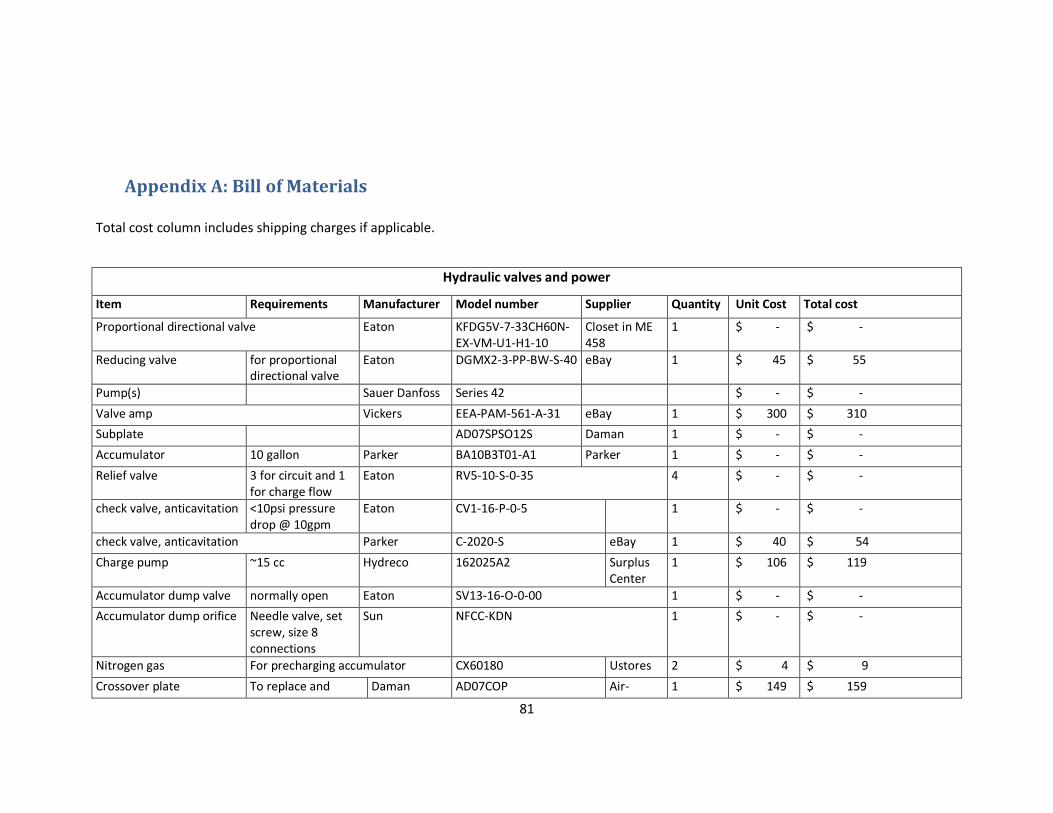
81
Appendix A: Bill of Materials
Total cost column includes shipping charges if applicable.
Hydraulic valves and power
Item Requirements Manufacturer Model number Supplier Quantity Unit Cost Total cost
Proportional directional valve Eaton KFDG5V-7-33CH60N-EX-VM-U1-H1-10
Closet in ME 458
1 $ - $ -
Reducing valve for proportional directional valve
Eaton DGMX2-3-PP-BW-S-40 eBay 1 $ 45 $ 55
Pump(s) Sauer Danfoss Series 42 $ - $ -
Valve amp Vickers EEA-PAM-561-A-31 eBay 1 $ 300 $ 310
Subplate AD07SPSO12S Daman 1 $ - $ -
Accumulator 10 gallon Parker BA10B3T01-A1 Parker 1 $ - $ -
Relief valve 3 for circuit and 1 for charge flow
Eaton RV5-10-S-0-35 4 $ - $ -
check valve, anticavitation <10psi pressure drop @ 10gpm
Eaton CV1-16-P-0-5 1 $ - $ -
check valve, anticavitation Parker C-2020-S eBay 1 $ 40 $ 54
Charge pump ~15 cc Hydreco 162025A2 Surplus Center
1 $ 106 $ 119
Accumulator dump valve normally open Eaton SV13-16-O-0-00 1 $ - $ -
Accumulator dump orifice Needle valve, set screw, size 8 connections
Sun NFCC-KDN 1 $ - $ -
Nitrogen gas For precharging accumulator CX60180 Ustores 2 $ 4 $ 9
Crossover plate To replace and Daman AD07COP Air- 1 $ 149 $ 159
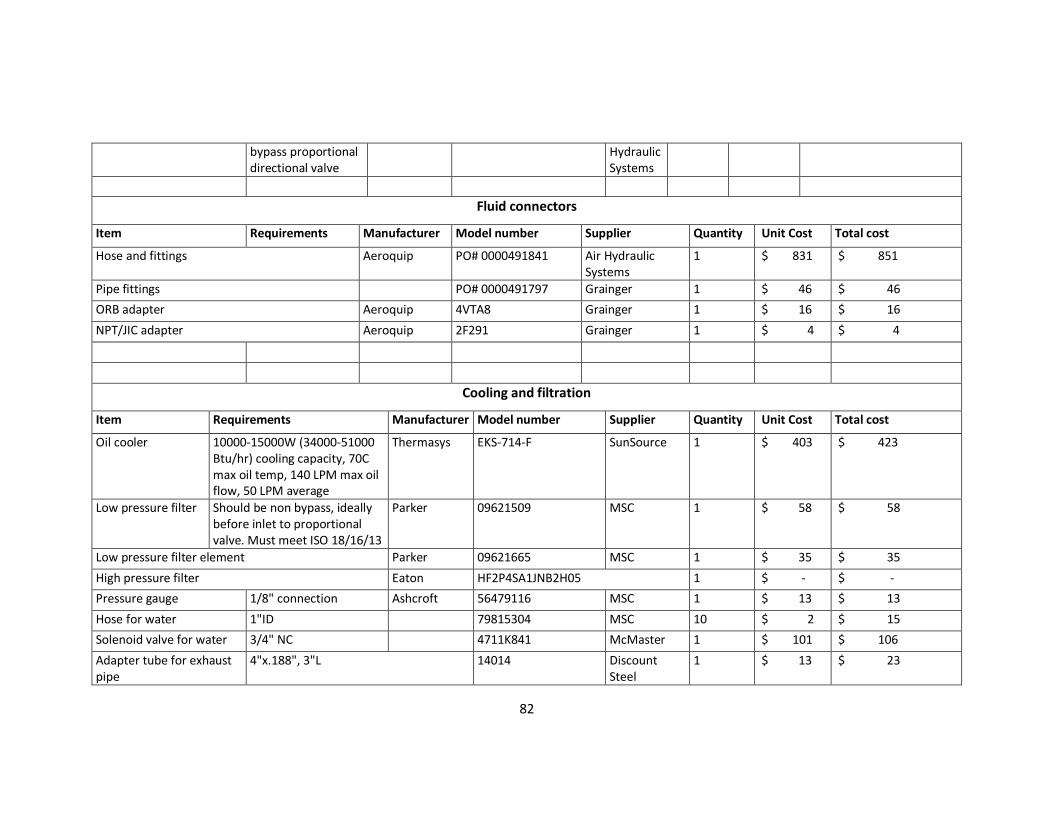
82
bypass proportional directional valve
Hydraulic Systems
Fluid connectors
Item Requirements Manufacturer Model number Supplier Quantity Unit Cost Total cost
Hose and fittings Aeroquip PO# 0000491841 Air Hydraulic Systems
1 $ 831 $ 851
Pipe fittings PO# 0000491797 Grainger 1 $ 46 $ 46
ORB adapter Aeroquip 4VTA8 Grainger 1 $ 16 $ 16
NPT/JIC adapter Aeroquip 2F291 Grainger 1 $ 4 $ 4
Cooling and filtration
Item Requirements Manufacturer Model number Supplier Quantity Unit Cost Total cost
Oil cooler 10000-15000W (34000-51000 Btu/hr) cooling capacity, 70C max oil temp, 140 LPM max oil flow, 50 LPM average
Thermasys EKS-714-F SunSource 1 $ 403 $ 423
Low pressure filter Should be non bypass, ideally before inlet to proportional valve. Must meet ISO 18/16/13
Parker 09621509 MSC 1 $ 58 $ 58
Low pressure filter element Parker 09621665 MSC 1 $ 35 $ 35
High pressure filter Eaton HF2P4SA1JNB2H05 1 $ - $ -
Pressure gauge 1/8" connection Ashcroft 56479116 MSC 1 $ 13 $ 13
Hose for water 1"ID 79815304 MSC 10 $ 2 $ 15
Solenoid valve for water 3/4" NC 4711K841 McMaster 1 $ 101 $ 106
Adapter tube for exhaust pipe
4"x.188", 3"L 14014 Discount Steel
1 $ 13 $ 23
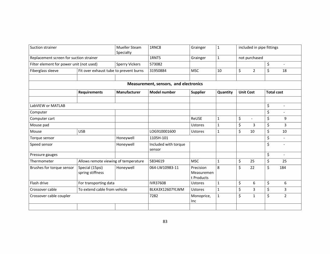
83
Suction strainer Mueller Steam Specialty
1RNC8 Grainger 1 included in pipe fittings
Replacement screen for suction strainer 1RNT5 Grainger 1 not purchased
Filter element for power unit (not used) Sperry Vickers 573082 $ -
Fiberglass sleeve Fit over exhaust tube to prevent burns 31950884 MSC 10 $ 2 $ 18
Measurement, sensors, and electronics
Requirements Manufacturer Model number Supplier Quantity Unit Cost Total cost
LabVIEW or MATLAB $ -
Computer $ -
Computer cart ReUSE 1 $ - $ 9
Mouse pad Ustores 1 $ 3 $ 3
Mouse USB LOG910001600 Ustores 1 $ 10 $ 10
Torque sensor Honeywell 1105H-101 $ -
Speed sensor Honeywell Included with torque sensor
$ -
Pressure gauges $ -
Thermometer Allows remote viewing of temperature 5834619 MSC 1 $ 25 $ 25
Brushes for torque sensor Special (15psi) spring stiffness
Honeywell 064-LW10983-11 Precision Measurement Products
8 $ 22 $ 184
Flash drive For transporting data IVR37608 Ustores 1 $ 6 $ 6
Crossover cable To extend cable from vehicle BLKA3X12607YLWM Ustores 1 $ 3 $ 3
Crossover cable coupler 7282 Monoprice, Inc
1 $ 1 $ 2
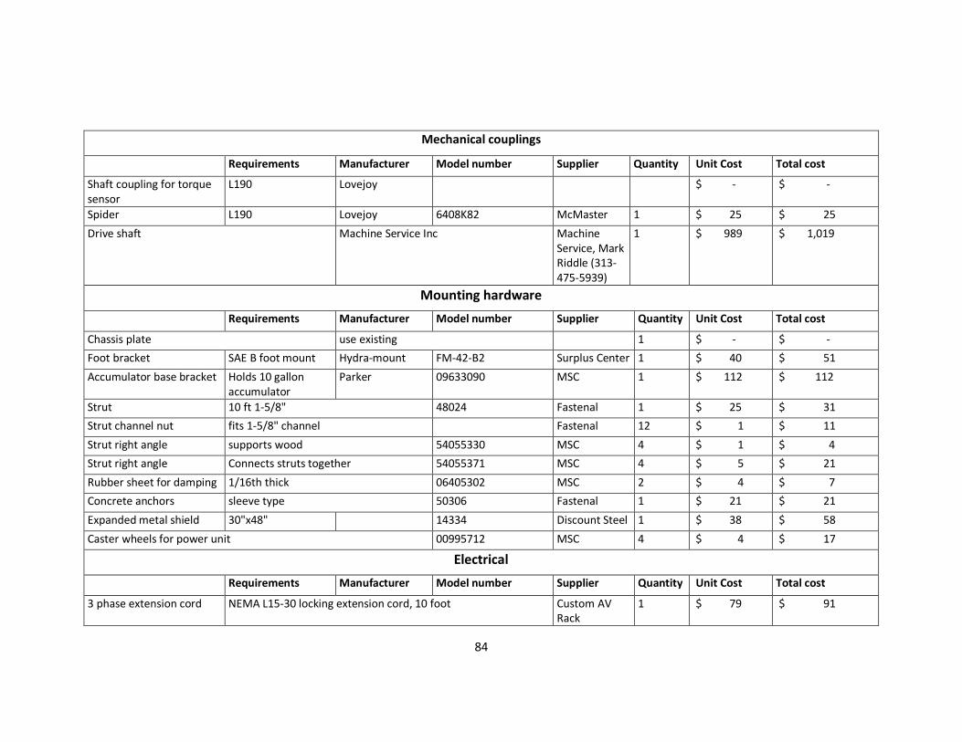
84
Mechanical couplings
Requirements Manufacturer Model number Supplier Quantity Unit Cost Total cost
Shaft coupling for torque sensor
L190 Lovejoy $ - $ -
Spider L190 Lovejoy 6408K82 McMaster 1 $ 25 $ 25
Drive shaft Machine Service Inc Machine Service, Mark Riddle (313-475-5939)
1 $ 989 $ 1,019
Mounting hardware
Requirements Manufacturer Model number Supplier Quantity Unit Cost Total cost
Chassis plate use existing 1 $ - $ -
Foot bracket SAE B foot mount Hydra-mount FM-42-B2 Surplus Center 1 $ 40 $ 51
Accumulator base bracket Holds 10 gallon accumulator
Parker 09633090 MSC 1 $ 112 $ 112
Strut 10 ft 1-5/8" 48024 Fastenal 1 $ 25 $ 31
Strut channel nut fits 1-5/8" channel Fastenal 12 $ 1 $ 11
Strut right angle supports wood 54055330 MSC 4 $ 1 $ 4
Strut right angle Connects struts together 54055371 MSC 4 $ 5 $ 21
Rubber sheet for damping 1/16th thick 06405302 MSC 2 $ 4 $ 7
Concrete anchors sleeve type 50306 Fastenal 1 $ 21 $ 21
Expanded metal shield 30"x48" 14334 Discount Steel 1 $ 38 $ 58
Caster wheels for power unit 00995712 MSC 4 $ 4 $ 17
Electrical
Requirements Manufacturer Model number Supplier Quantity Unit Cost Total cost
3 phase extension cord NEMA L15-30 locking extension cord, 10 foot Custom AV Rack
1 $ 79 $ 91
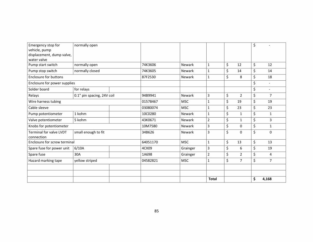
85
Emergency stop for vehicle, pump displacement, dump valve, water valve
normally open $ -
Pump start switch normally open 74K3606 Newark 1 $ 12 $ 12
Pump stop switch normally closed 74K3605 Newark 1 $ 14 $ 14
Enclosure for buttons 87F2530 Newark 1 $ 8 $ 18
Enclosure for power supplies $ -
Solder board for relays $ -
Relays 0.1" pin spacing, 24V coil 94B9941 Newark 3 $ 2 $ 7
Wire harness tubing 01578467 MSC 1 $ 19 $ 19
Cable sleeve 03080074 MSC 1 $ 23 $ 23
Pump potentiometer 1 kohm 10C0280 Newark 1 $ 1 $ 1
Valve potentiometer 5 kohm 43K0671 Newark 2 $ 1 $ 3
Knobs for potentiometer 10M7580 Newark 3 $ 0 $ 1
Terminal for valve LVDT connection
small enough to fit 34B626 Newark 3 $ 0 $ 0
Enclosure for screw terminal 64051170 MSC 1 $ 13 $ 13
Spare fuse for power unit 6/10A 4CX09 Grainger 3 $ 6 $ 19
Spare fuse 30A 1A698 Grainger 2 $ 2 $ 4
Hazard marking tape yellow striped 04582821 MSC 1 $ 7 $ 7
Total $ 4,168
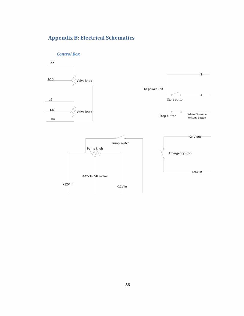
86
Appendix B: Electrical Schematics
Control Box
Valve knob
Valve knob
b2
b10
z2
b6
b4
Pump switch
Pump knob
-12V in+12V in
0-12V for S42 control
Emergency stop
+24V out
+24V in
Start button
Stop button
3
4
Where 3 was onexisting button
To power unit
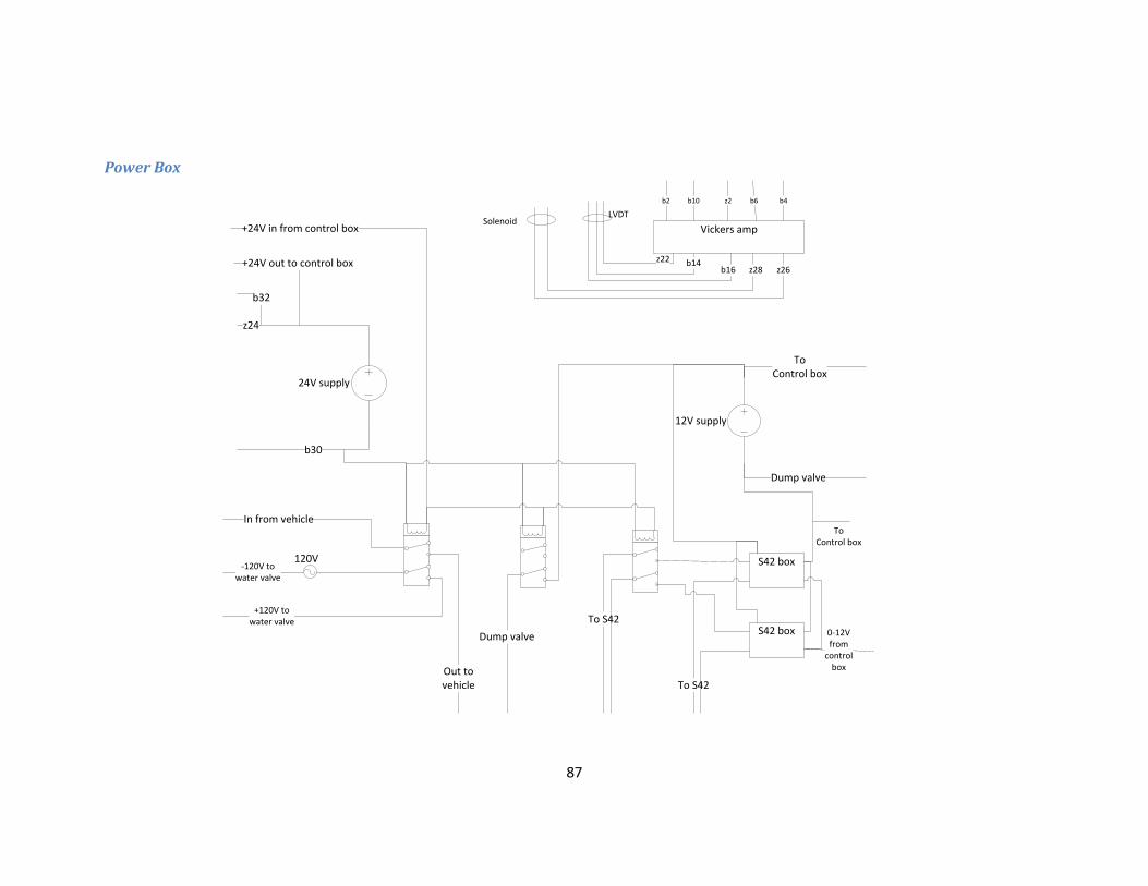
87
Power Box
24V supply
120V
12V supply
Vickers amp
S42 box
S42 box
b30
z24
b32
+24V out to control box
+24V in from control box
-120V towater valve
+120V towater valve
In from vehicle
Out tovehicle
Dump valve
ToControl box
To S42
To S42
0-12Vfrom
controlbox
Dump valve
ToControl box
b2 b10 z2 b6 b4
z22 b14b16 z28 z26
LVDTSolenoid
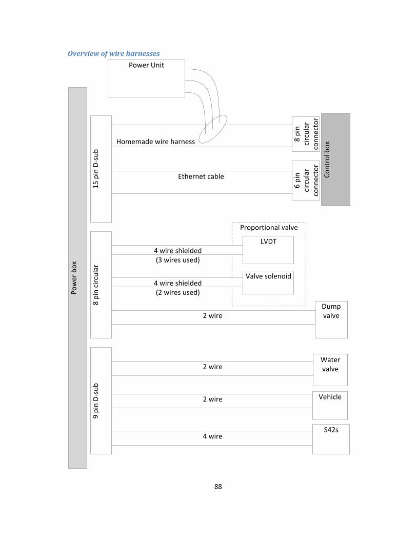
88
Overview of wire harnesses
2 wire
2 wire
4 wire
2 wire
Proportional valve
4 wire shielded(3 wires used)
4 wire shielded(2 wires used)
Homemade wire harness
Ethernet cable
Po
wer
bo
x
15
pin
D-s
ub
8 p
in c
ircu
lar
9 p
in D
-su
b
Co
ntr
ol b
ox
Power Unit
8 p
in
circ
ula
rco
nn
ecto
r
6 p
in
circ
ula
rco
nn
ecto
r
LVDT
Valve solenoid
Dump valve
Water valve
Vehicle
S42s
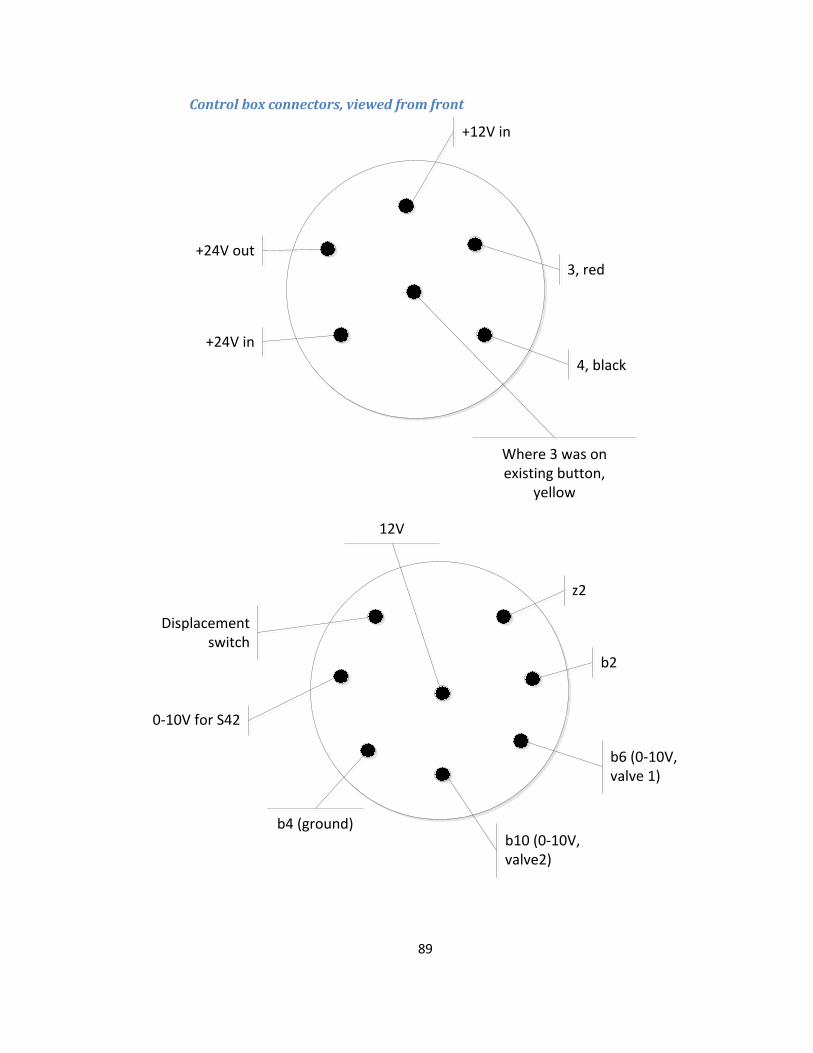
89
Control box connectors, viewed from front
4, black
3, red
+12V in
+24V out
+24V in
z2
b2
b6 (0-10V, valve 1)
b10 (0-10V, valve2)
b4 (ground)
0-10V for S42
Displacement switch
12V
Where 3 was on existing button,
yellow
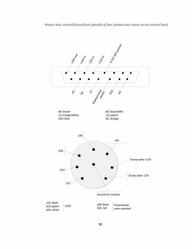
90
Power box, viewed from front outside of box (names are same as on control box)
b4: brownz2: orange/whiteb10: blue
b6: blue/whitez11: greenb2: orange
z22: blackb14: greenb16: white
z28: blackZ26: red
+24V
out
+24V
in
-12V
in
+12V
in
0-12
V S4
2 co
ntro
lb2b1
0
Dis
plac
emen
t sw
itch
b6b4 z2
z22
b14
b16
z28
z26
Dump valve +12V
Dump valve -12V
Ground for screens
LVDT Proportional valve soleniod
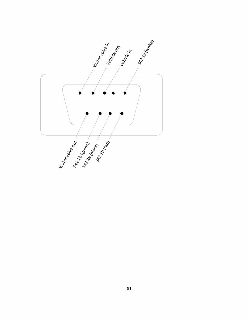
91
Wat
er v
alve
inVe
hicl
e ou
tVe
hicl
e in
S42
1a (w
hite
)
Wat
er v
alve
out
S42
2b (g
reen
)S4
2 2a
(bla
ck)
S42
1b (r
ed)
92
Appendix C: Torque Sensor Calibration Instructions
1. Manually rotate the driveshaft to zero torque.
2. Open grey Honeywell in-line amplifier box.
3. The blue potentiometers are zeros. Turn the screws on them such that the torque
measurement on the screen shows zero.
4. Flip the top switch on the black aluminum connector box to up.
5. Turn the grey (span fine-control) such that the torque measurement on screen shows
390.55Nm.
6. Flip the switch back down.
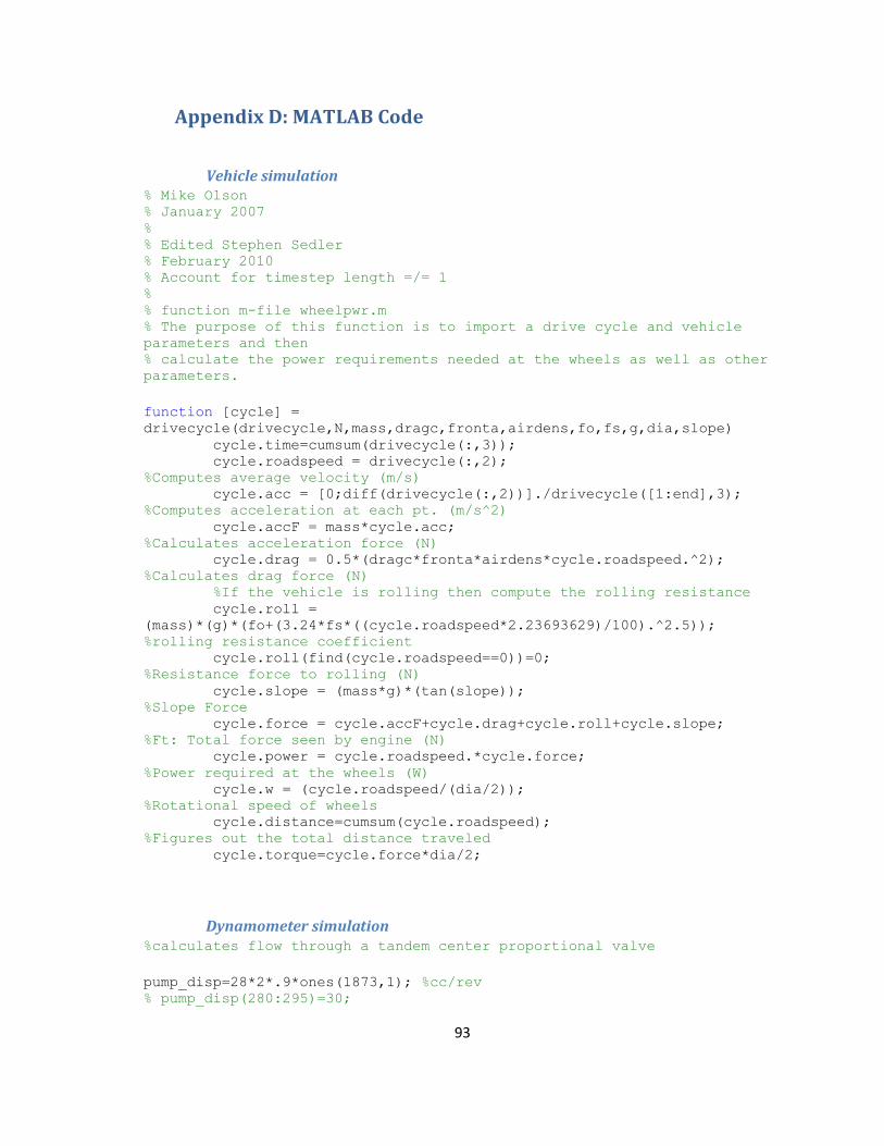
93
Appendix D: MATLAB Code
Vehicle simulation % Mike Olson % January 2007 % % Edited Stephen Sedler % February 2010 % Account for timestep length =/= 1 % % function m-file wheelpwr.m % The purpose of this function is to import a drive cycle and vehicle
parameters and then % calculate the power requirements needed at the wheels as well as other
parameters.
function [cycle] =
drivecycle(drivecycle,N,mass,dragc,fronta,airdens,fo,fs,g,dia,slope) cycle.time=cumsum(drivecycle(:,3)); cycle.roadspeed = drivecycle(:,2);
%Computes average velocity (m/s) cycle.acc = [0;diff(drivecycle(:,2))]./drivecycle([1:end],3);
%Computes acceleration at each pt. (m/s^2) cycle.accF = mass*cycle.acc;
%Calculates acceleration force (N) cycle.drag = 0.5*(dragc*fronta*airdens*cycle.roadspeed.^2);
%Calculates drag force (N) %If the vehicle is rolling then compute the rolling resistance cycle.roll =
(mass)*(g)*(fo+(3.24*fs*((cycle.roadspeed*2.23693629)/100).^2.5));
%rolling resistance coefficient cycle.roll(find(cycle.roadspeed==0))=0;
%Resistance force to rolling (N) cycle.slope = (mass*g)*(tan(slope));
%Slope Force cycle.force = cycle.accF+cycle.drag+cycle.roll+cycle.slope;
%Ft: Total force seen by engine (N) cycle.power = cycle.roadspeed.*cycle.force;
%Power required at the wheels (W) cycle.w = (cycle.roadspeed/(dia/2));
%Rotational speed of wheels cycle.distance=cumsum(cycle.roadspeed);
%Figures out the total distance traveled cycle.torque=cycle.force*dia/2;
Dynamometer simulation %calculates flow through a tandem center proportional valve
pump_disp=28*2*.9*ones(1873,1); %cc/rev % pump_disp(280:295)=30;
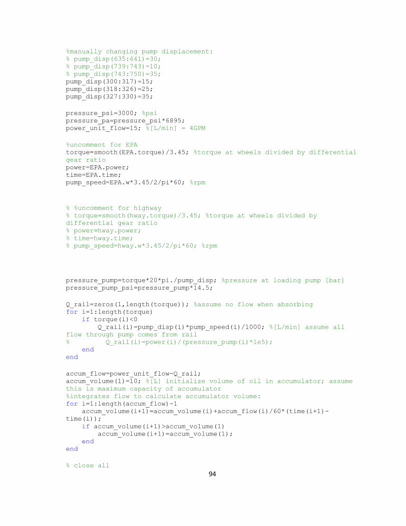
94
%manually changing pump displacement: % pump_disp(635:641)=30; % pump_disp(739:743)=10; % pump_disp(743:750)=35; pump_disp(300:317)=15; pump_disp(318:326)=25; pump_disp(327:330)=35;
pressure_psi=3000; %psi pressure_pa=pressure_psi*6895; power_unit_flow=15; %[L/min] = 4GPM
%uncomment for EPA torque=smooth(EPA.torque)/3.45; %torque at wheels divided by differential
gear ratio power=EPA.power; time=EPA.time; pump_speed=EPA.w*3.45/2/pi*60; %rpm
% %uncomment for highway % torque=smooth(hway.torque)/3.45; %torque at wheels divided by
differential gear ratio % power=hway.power; % time=hway.time; % pump_speed=hway.w*3.45/2/pi*60; %rpm
pressure_pump=torque*20*pi./pump_disp; %pressure at loading pump [bar] pressure_pump_psi=pressure_pump*14.5;
Q_rail=zeros(1,length(torque)); %assume no flow when absorbing for i=1:length(torque) if torque(i)<0 Q_rail(i)=pump_disp(i)*pump_speed(i)/1000; %[L/min] assume all
flow through pump comes from rail % Q_rail(i)=power(i)/(pressure_pump(i)*1e5); end end
accum_flow=power_unit_flow-Q_rail; accum_volume(1)=10; %[L] initialize volume of oil in accumulator; assume
this is maximum capacity of accumulator
%integrates flow to calculate accumulator volume: for i=1:length(accum_flow)-1 accum_volume(i+1)=accum_volume(i)+accum_flow(i)/60*(time(i+1)-
time(i)); if accum_volume(i+1)>accum_volume(1) accum_volume(i+1)=accum_volume(1); end end
% close all
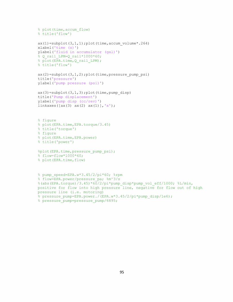
95
% plot(time,accum_flow) % title('flow')
ax(1)=subplot(3,1,1);plot(time,accum_volume*.264) xlabel('time (s)') ylabel('fluid in accumulator (gal)') % Q_rail_LPM=Q_rail*1000*60; % plot(EPA.time,Q_rail_LPM); % title('flow')
ax(2)=subplot(3,1,2);plot(time,pressure_pump_psi) title('pressure') ylabel('pump pressure (psi)')
ax(3)=subplot(3,1,3);plot(time,pump_disp) title('Pump displacement') ylabel('pump disp (cc/rev)') linkaxes([ax(3) ax(2) ax(1)],'x');
% figure % plot(EPA.time,EPA.torque/3.45) % title('torque') % figure % plot(EPA.time,EPA.power) % title('power')
%plot(EPA.time,pressure_pump_psi); % flow=flow*1000*60; % plot(EPA.time,flow)
% pump_speed=EPA.w*3.45/2/pi*60; %rpm % flow=EPA.power/pressure_pa; %m^3/s
%(abs(EPA.torque)/3.45)*60/2/pi*pump_disp*pump_vol_eff/1000; %L/min,
positive for flow into high pressure line, negative for flow out of high
pressure line (i.e. motoring) % pressure_pump=EPA.power./(EPA.w*3.45/2/pi*pump_disp/1e6); % pressure_pump=pressure_pump/6895;
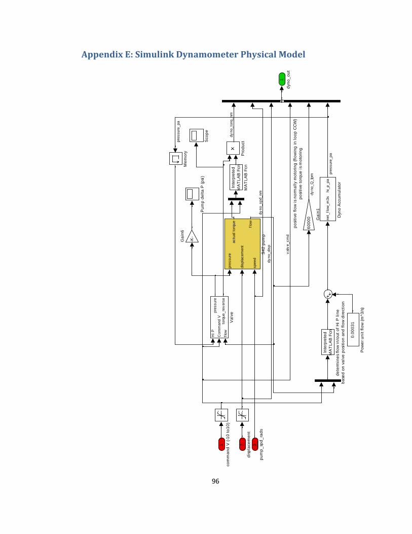
96
Appendix E: Simulink Dynamometer Physical Model
po
siti
ve
flo
w i
s n
orm
all
y m
oto
rin
g (
flo
win
g i
n l
oo
p C
CW
)
po
siti
ve
to
rqu
e i
s m
oto
rin
g
1
dyn
o_
ou
t
Inte
rpre
ted
MA
TL
AB
Fcn
de
term
ine
s fl
ow
in
/ou
t o
f H
i P
lin
e
ba
sed
on
va
lve
po
siti
on
an
d f
low
dir
ecti
on
Hi P
Co
mm
and
V
flo
w
pre
ssu
re
torq
ue_
rev
ers
e
Va
lve
Sco
pe
pre
ssu
re
dis
pla
ce
me
nt
sp
ee
d
actu
al to
rqu
e
flo
w
S4
2 p
um
p
Pu
mp
de
lta
P (
psi
)
Pro
du
ct
0.0
00
31
Po
we
r u
nit
flo
w (
m^3
/s)
Me
mo
ry
Inte
rpre
ted
MA
TL
AB
Fcn
MA
TL
AB
Fcn
-K-
Ga
in6
60
00
0 Ga
in1
net_
flo
w_
m3
sh
i_p
_p
a
Dyn
o A
ccu
mu
lato
r
3
pu
mp
_sp
d_
rad
s
2
dis
pla
ce
me
nt
1
co
mm
an
d V
(-1
0 t
o1
0)
pre
ssu
re_
pa
pre
ssu
re_
pa
dy
no_
sp
d_
nm
dy
no_
dis
p
va
lve
_cm
d
dy
no_
torq
_nm
dy
no_
Q_
lpm
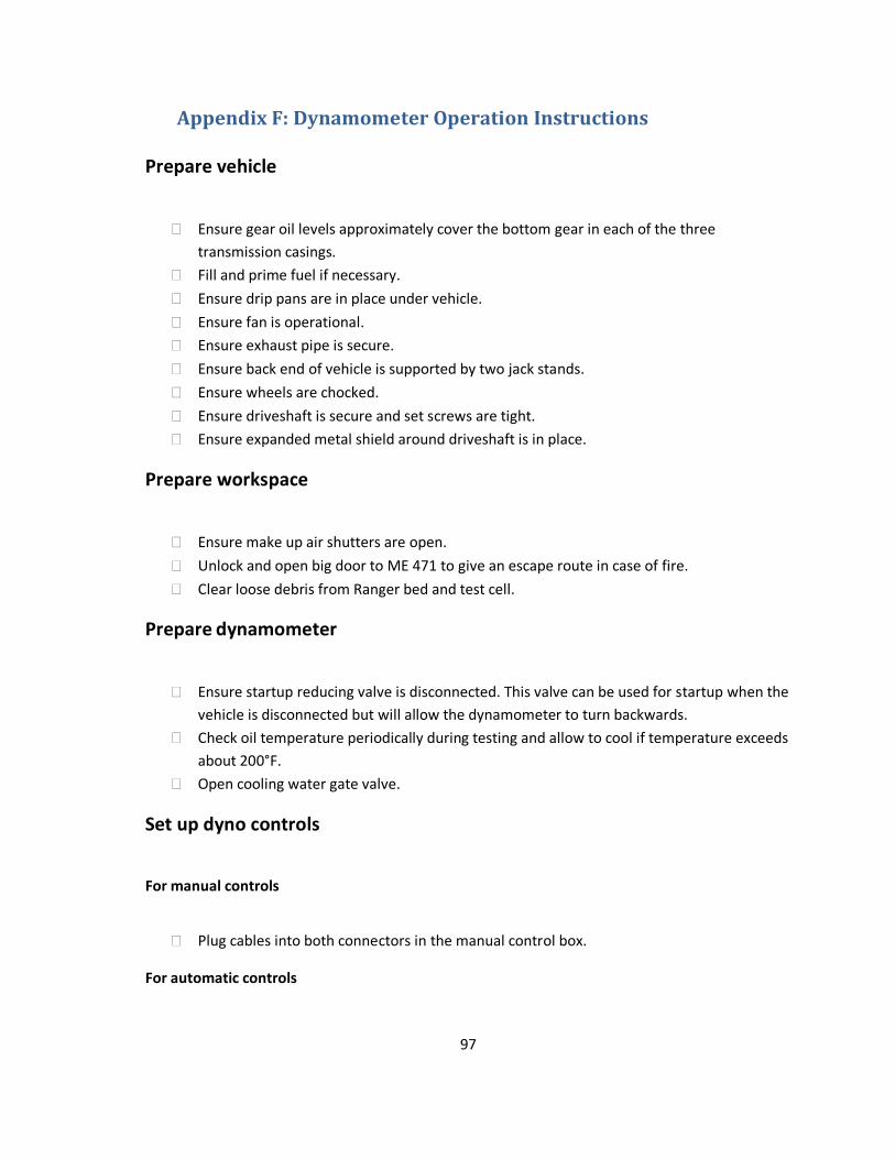
97
Appendix F: Dynamometer Operation Instructions
Prepare vehicle
Ensure gear oil levels approximately cover the bottom gear in each of the three
transmission casings.
Fill and prime fuel if necessary.
Ensure drip pans are in place under vehicle.
Ensure fan is operational.
Ensure exhaust pipe is secure.
Ensure back end of vehicle is supported by two jack stands.
Ensure wheels are chocked.
Ensure driveshaft is secure and set screws are tight.
Ensure expanded metal shield around driveshaft is in place.
Prepare workspace
Ensure make up air shutters are open.
Unlock and open big door to ME 471 to give an escape route in case of fire.
Clear loose debris from Ranger bed and test cell.
Prepare dynamometer
Ensure startup reducing valve is disconnected. This valve can be used for startup when the
vehicle is disconnected but will allow the dynamometer to turn backwards.
Check oil temperature periodically during testing and allow to cool if temperature exceeds
about 200°F.
Open cooling water gate valve.
Set up dyno controls
For manual controls
Plug cables into both connectors in the manual control box.
For automatic controls
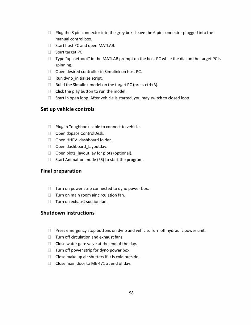
98
Plug the 8 pin connector into the grey box. Leave the 6 pin connector plugged into the
manual control box.
Start host PC and open MATLAB.
Start target PC
Type "xpcnetboot" in the MATLAB prompt on the host PC while the dial on the target PC is
spinning.
Open desired controller in Simulink on host PC.
Run dyno_initialize script.
Build the Simulink model on the target PC (press ctrl+B).
Click the play button to run the model.
Start in open loop. After vehicle is started, you may switch to closed loop.
Set up vehicle controls
Plug in Toughbook cable to connect to vehicle.
Open dSpace ControlDesk.
Open HHPV_dashboard folder.
Open dashboard_layout.lay.
Open plots_layout.lay for plots (optional).
Start Animation mode (F5) to start the program.
Final preparation
Turn on power strip connected to dyno power box.
Turn on main room air circulation fan.
Turn on exhaust suction fan.
Shutdown instructions
Press emergency stop buttons on dyno and vehicle. Turn off hydraulic power unit.
Turn off circulation and exhaust fans.
Close water gate valve at the end of the day.
Turn off power strip for dyno power box.
Close make up air shutters if it is cold outside.
Close main door to ME 471 at end of day.