Lab 9: FTT and power spectra

The Fast Fourier Transform (FFT) is a fast and efficient numerical algorithmthat computes the Fourier transform. The power spectrum is a plot of the power,or variance, of a time series as a function of the frequency1. If G(f) is the Fouriertransform, then the power spectrum, W (f), can be computed as

W (f) = |G(f)| = G(f)G∗(f)

where G∗(f) is the complex conjugate of G(f). We refer to the power spectrumcalculated in this way as the periodogram.

Currently, many investigators prefer to estimate the power spectral density us-ing matplotlib.mlab.psd(). This method is based on Welch’s averagedperiodogram method. Welch’s method reduces noise in the estimated spectrum atthe expense of reducing the frequency resolution (see below). For many of the ex-perimental uses of power spectra, the advantages of reducing the effects of noiseout-weigh the dis-advantages of reduced frequency resolution. As we showed inlecture there is little practiacl difference between determining the periodogramversus the power spectral density. However, the flexibility of mlab.psd() pro-vides esufficient motivation to learn how to use this package.

Often overlooked is that the fact that W (f) is the power spectrum obtainedfor an infinitely long time series measured with infinitely fine precision. In con-trast, in the laboratory we work with time series of finite length that are subjectedto uncorrelated, random inputs (noise) and effects introduced by the process ofmeasuring the signal.

The purpose of this laboratory is to illustrate the use of mlab.psd() andexplore a number of applications of the FFT and power spectra.

1For simplicity we have assumed that the independent variable is time; however, it could alsobe a spatial dimension. We use the term power spectra as a collective term to include both theperiodogram and the power spectral density.

1

Browser: Essentially everything that you would ever want to know about theuses of the FFT can be located on the Internet by asking the right questions. InPython, the functions necessary to calculate the FFT are located in the numpylibrary called fft. If we want to use the function fft(), we must add thefollowing command to the top matter of our program:

import numpy.fft as fft

Thus, the command for determining the FFT of a signal x(t) becomes fft.fft(x).Of course, you could import the fft-package from numpy under a differentname; however, this might make the program less readable by others. Otherfunctions related to the use of the FFT are located in scipy such as the librarysignal, i.e.

import scipy.signal as signal

The description of each command and how to use it can easily be obtained by us-ing your web browser and typing the name of the library together with the functionthat you want to know about.

House keeping: Today we will illustrate the applications of the FFT and thepower spectra by working with real data. The deliverables take the form of fig-ures prepared using Matplotlib. We suggest that you create a directory foreach figure which contains both the data and the program(s) used to generate therequired figure. This is actually a good habit to acquire. One advantage is thatyou don’t need to worry about specifying the required paths since, by default, aPython program looks first in the directory they are running for required inputfiles. A second advantage occurs if, my goodness, you actually need to modifyyour figure at a later date following comments made by a grader or a reviewer ofyour article (senior thesis, publications, book).

1 BackgroundWe illustrate the difference between W (f) and w(f) by calculating the powerspectrum of x(t) = sin(2πf0t), where f0 is a particular frequency. By definition,the Fourier transform of sin(2πft) is

G(sin 2πf0t)(f) =

∫ ∞−∞

e−2πjft sin 2πf0tdt (1)

2

where we have distinguished a particular value of the frequency, f , as f0. UsingEuler’s relation, we can write

sin 2πf0t =e2πjf0t − e−2πjf0t

2j

Substituting into (1), we obtain

G(sin 2πf0t)(f) =

∫ ∞−∞

e−2πjft

[e2πjf0t − e−2πjf0t

2j

]dt

=1

2j

∫ ∞−∞

[e−2πj(f−f0)t − e−2πj(f+f0)t

]dt

=1

2j[δ(f − f0)− δ(f + f0)]

=j

2[δ(f + f0)− δ(f − f0)]

Here we see that both the Fourier transform and the power spectrum, W (f), ofsin(2πft) are predicted to be composed of two delta-functions, one centered at+f0 and the other at −f0.

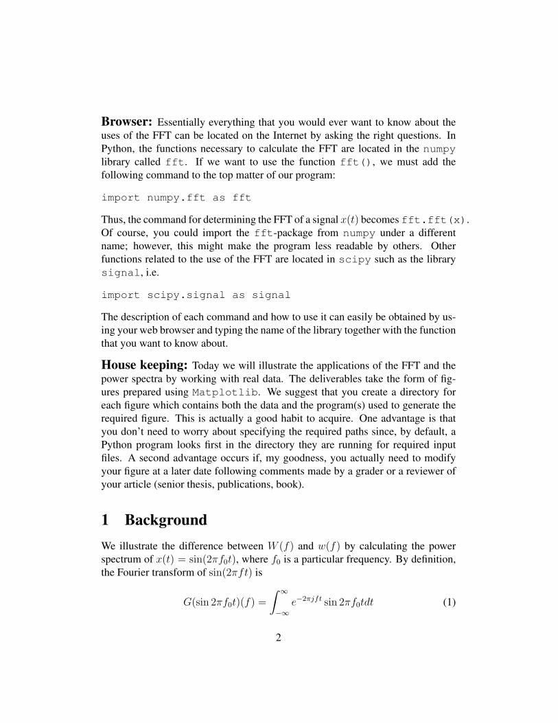
Figure 1: Computer screen shot obtained after typing python at the Commandprompt. The three >>> means that we are operating in script mode.

Now let’s use Python to compute the FFT and the power spectrum, w(f).Python can be run directly from the command line, namely in an interactive mode2

(a much more powerful and popular version of interactive Python programming

2Up to now we have run Python in its script mode, namely, we write computer program,name.py and then run the program by typing python name.py (Did you remember to addthe & ?). There are two advantages: 1) we can use the same program over and over again, and 2)the program gives us a permanent record of what we did. However, the interactive mode is usefulwhen the goal is simply to explore data.

3

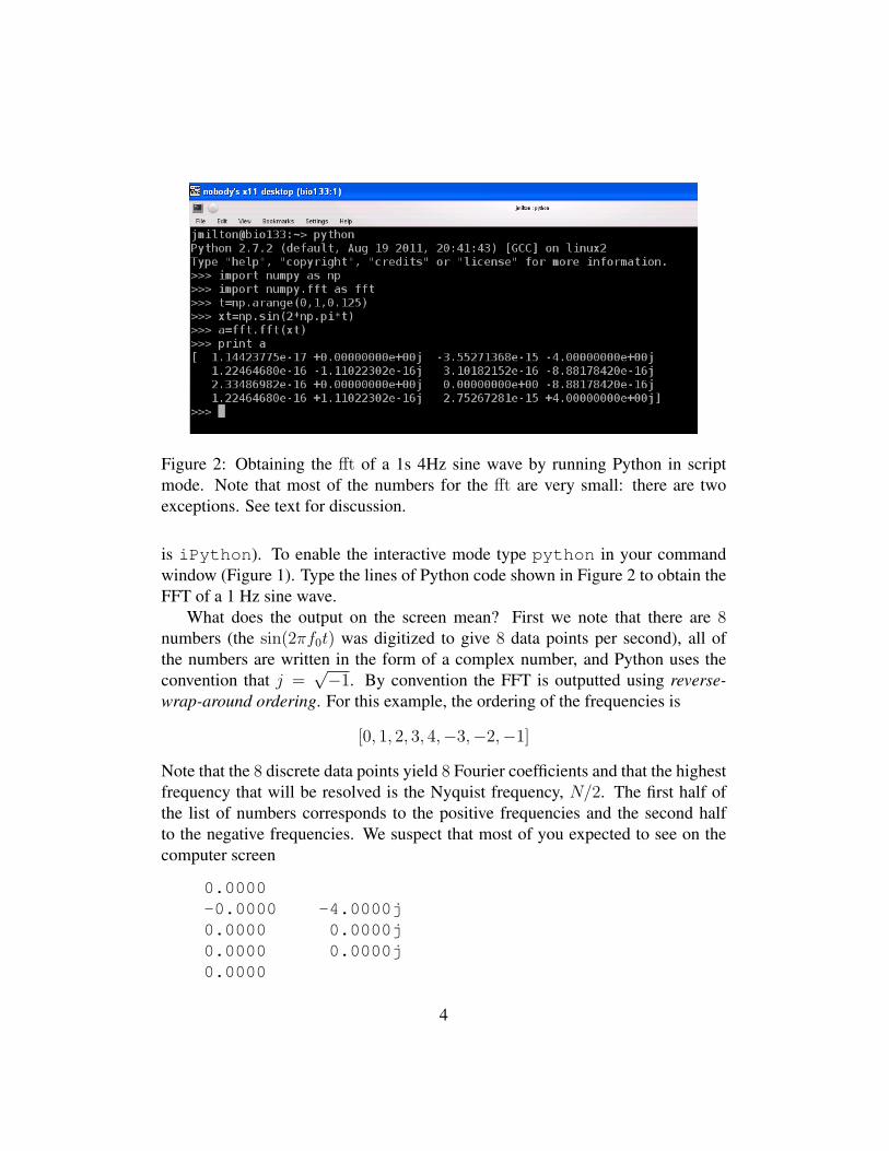
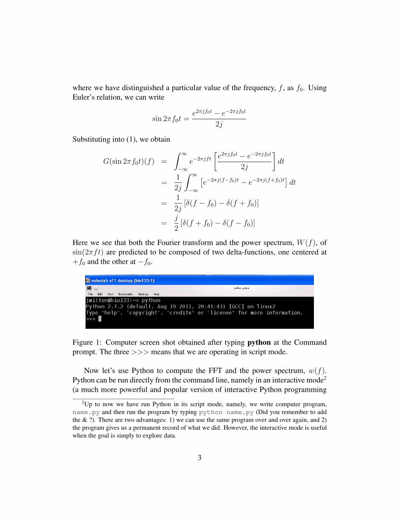
Figure 2: Obtaining the fft of a 1s 4Hz sine wave by running Python in scriptmode. Note that most of the numbers for the fft are very small: there are twoexceptions. See text for discussion.

is iPython). To enable the interactive mode type python in your commandwindow (Figure 1). Type the lines of Python code shown in Figure 2 to obtain theFFT of a 1 Hz sine wave.

What does the output on the screen mean? First we note that there are 8numbers (the sin(2πf0t) was digitized to give 8 data points per second), all ofthe numbers are written in the form of a complex number, and Python uses theconvention that j =

√−1. By convention the FFT is outputted using reverse-

wrap-around ordering. For this example, the ordering of the frequencies is

[0, 1, 2, 3, 4,−3,−2,−1]

Note that the 8 discrete data points yield 8 Fourier coefficients and that the highestfrequency that will be resolved is the Nyquist frequency, N/2. The first half ofthe list of numbers corresponds to the positive frequencies and the second halfto the negative frequencies. We suspect that most of you expected to see on thecomputer screen

0.0000-0.0000 -4.0000j0.0000 0.0000j0.0000 0.0000j0.0000

4

0.0000 0.0000j0.0000 0.0000j-0.0000 +4.0000j

However, notice that many of the numbers are very, very small, for example of theorder 10−17. These numbers simply represent numerical noise in the computer. Ifwe set mentally all numbers< 10−3 equal to 0, then we obtain the expected result.

It should be noted that recent releases of numpy.fft include the commandsrfft() and irfft(). The advantage of using rfft() over fft() becomesof practical importance when we consider a problem that can arise when we com-pute the inverse FFT using ifft(). Since we typically have a real signal, weexpect that the inverse should also be real. However, it can happen, due to round-ing errors, that ifft() contains complex numbers. The use of rfft() avoidsthis problem.

Thanks to the development of computer software packages, such as MATLAB,Mathematica, Octave and Python, this task has become much easier. A particu-larly useful function is Python’s matplotlob.mlab.psd() developed by thelate John D. Hunter3

matplotlib.mlab.psd(x, NFFT, Fs, detrend, window,noverlap=0, pad_to, sides=, scale_by_freq)

It is important to keep in mind that psd() does not calculate the periodogram,but calculates the power spectral density using a mathematical method knownas Welch’s method. The advantages of using mlab.psd() are that it is veryversatile and for everyday use we can accept the default choices for most of theoptions.

2 Exercise 1: Computing the power spectral densityusing mlab.psd()

2.1 Power Spectral Density RecipeIn the not too distant past, obtaining proper power spectra was a task that wasbeyond the capacity of most biologists4. However, thanks to the development

3We strongly recommend that readers do not use pylab’s version of psd(). The mat-plolib.mlab.psd() produces the same power spectrum as obtained using the corresponding pro-grams in MATLAB.

4For convenience we reproduce Section 8.4.5 here.

5

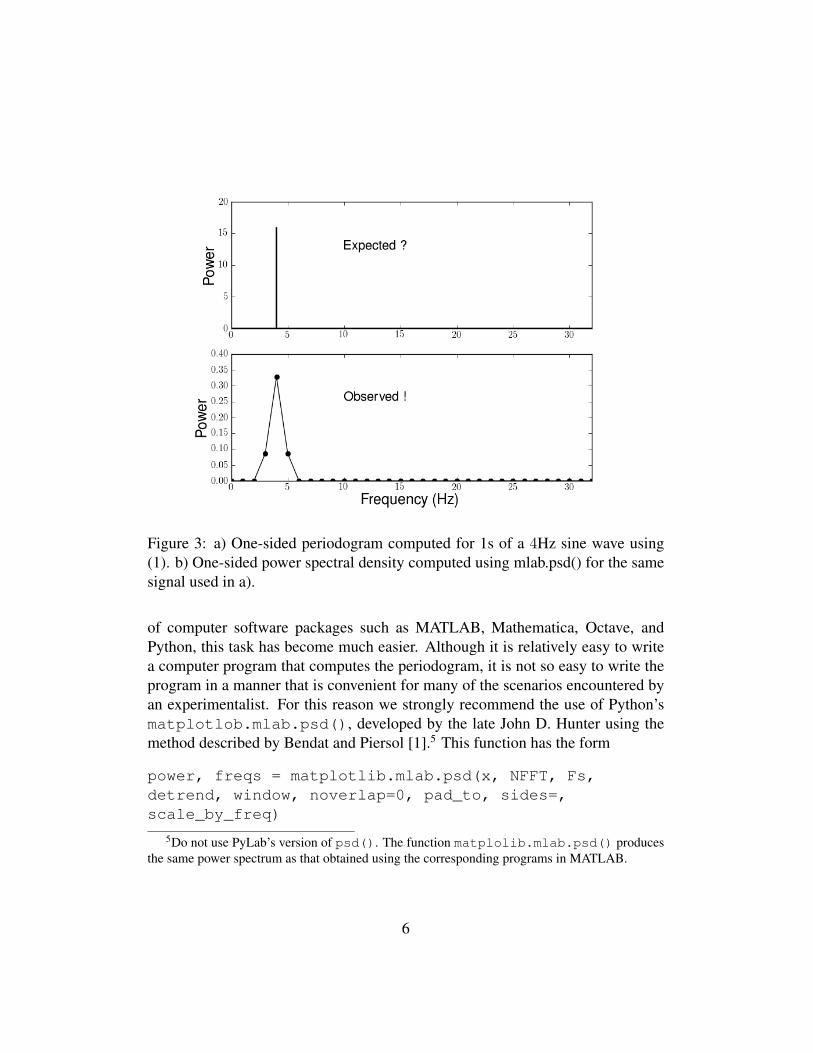
Figure 3: a) One-sided periodogram computed for 1s of a 4Hz sine wave using(1). b) One-sided power spectral density computed using mlab.psd() for the samesignal used in a).

of computer software packages such as MATLAB, Mathematica, Octave, andPython, this task has become much easier. Although it is relatively easy to writea computer program that computes the periodogram, it is not so easy to write theprogram in a manner that is convenient for many of the scenarios encountered byan experimentalist. For this reason we strongly recommend the use of Python’smatplotlob.mlab.psd(), developed by the late John D. Hunter using themethod described by Bendat and Piersol [1].5 This function has the form

power, freqs = matplotlib.mlab.psd(x, NFFT, Fs,detrend, window, noverlap=0, pad_to, sides=,scale_by_freq)

5Do not use PyLab’s version of psd(). The function matplolib.mlab.psd() producesthe same power spectrum as that obtained using the corresponding programs in MATLAB.

6

The output is two one-dimensional arrays, one of which gives the values of thepower in db Hz−1, the other the corresponding values of the frequency.

The advantage of matplotlib.mlab.psd() is its versatility. Assumingthat an investigator has available a properly low-pass-filtered time signal, the stepsfor obtaining the power density density are as follows:

1. Enter the filtered and discretely sampled time signal x(t).

2. The number of points per data block is NFFT. NFFT must be an even num-ber. The computation is most efficient if NFFT = 2n, where n a positiveinteger; however, with modern laptops, the calculations when NFFT 6= 2n

are performed quickly.

3. Enter Fs. This parameter scales the frequency axis on the interval [0, Fs/2],where Fs/2 is the Nyquist frequency.

4. Enter the detrend option. Recall that it this a standard procedure to removethe mean from the time series before computing the power spectrum.

5. Enter the windowing option. Keep in mind that using a windowing functionis better than not using one, and from a practical point of view, there islittle difference among the various windowing functions. The default is theHanning windowing function.

6. Typically accept the overlap default choice of 0 (see below for moredetails).

7. Choose pad to (see below). The default is 0.

8. Choose the number of sides. The default for real data is a one-sided powerspectrum.

9. Choose scale by freq. Typically, you will choose the default, since thatmakes the power spectrum compatible with that obtained using MATLAB.

The versatility of mlab.psd() resides in the interplay between the optionsNFFT, noverlap and pad to. The following scenarios illustrate the salientpoints for signals for which the mean has been removed.

1. Frequencies greater than 1 Hz: The options available depend on the lengthof x, L(x). If L(x) = NFFT, then the time is 1 sec and we can accept thedefaults and the command to produce the power spectrum. For example,when the digitization rate is 256 points per second the command would be

7

mlab.psd(x,256,256)

We can increase the resolution by using the pad to option. For example fora sample initially digitzied at 256 Hz, we can calculate the power spectrumfor a 512 Hz digitization rate by using the command

mlab.psd(x,256,512,pad_to=512)

Finally we can average the time series by taking x to be an integer mutipleof NFFT, Xn. This prodedure is useful when data is noisy and when wewant to use the noverlap option in addition to windowing to minimizepower leakage. Thus the command takes the form

mlab.psd(X_n,256,256,noverlap=128)

It should be noted that the optimal choice for noverlap is one-half ofNFFT, namely the length of the time series, including zero padding.

2. Frequencies less than 1 Hz: It is necessary to first determine the minimallength of time series that is required. Suppose we wanted to look for pe-riodic components of the order of 0.1Hz. A 0.1Hz sinusoidal rhythm willhave 1 cycle every 10 seconds. Thus the length of time series must be atleast 10 seconds long. However, we will clearly get a much better lookingpower spectrum the longer the time series so maybe we should use 10 timeslonger, e.g. 100s. Thus the command becomes

mlab.psd(x,6400,64)

It is important to note that the characterization of the frequency content ofbiological time series in the less than 1 Hz freqnecy range is made problem-atic because of the effects of non-stationarity. Thus the length of the timeseries and often the particular segment of the time series to be analyzedmust be chosen with great care. In fact, it is in the analysis of such timeseries that many of the options available in mlab.psd() are most useful.

8

2.2 Example using mlab.psd()Figure 3 shows the power spectrum determined for 1s of a 4 Hz sine wave sam-pled at 64 Hz. Note that we have plotted the results using a linear scale for bothaxis. What is the Nyquist frequency? It is 64/2 = 32 Hz. The periodogram isshown in Figure 3a. We obtained the periodogram by squaring (term-by-term) thefft shown in Figure 2. Since values except those at ±4Hz are zero we get twodelta-functions, each with with height 16. We have plotted the one-sided powerspectrum.

The power spectral density is shown in Figure 3b. The power spectral densitylooks different than the periodogram. Although both are centered at the expected4Hz, the power spectral density is broader than the periodogram. A rough esti-mate of the frequency resolution of a pure frequency in the power spectrum is thewidth of the peak at one-half height: the bigger the half width the lower the fre-quency resolution. Thus the increased width of the 4Hz peak in Figure 3b reflectsthe decrease in frequency resolution obtained when on uses Welch’s method toestimate the power spectral density. Keep in mind that the advantage of Welch’smethod occurs when we have imperfect data of finite length subjected to randomperturbations.

Figure 4 shows the loglog plots of the power spectra shown in Figure 3. Wesuspect that most of you are surprised by the appearance of loglog plot of thepower spectral density. Why does it look this way? To answer this question it isimportant to remember that the power spectrum is actually being computed forthe signal that has been filtered using the rectangular sampling function. Thusthe power spectrum of a discrete frequency will resemble sinc(f). The reasonthat the ripples of the sinc function are not apparent is because of the averag-ing (smoothing) that is part of Welch’s method to determine the power spectraldensity.

Questions to be answered:1. Frequency resolution: The frequency resolution of the power spectral den-

sity can be increased by increasing the length of the time series. In mlab.psd()we can increase the sample length by increasing the number of points in thedata block, i.e. by changing NFFT, but by keeping Fs the same. For exam-ple, if we had 10s of a 4Hz sine wave sampled at 64Hz, then NFFT =640 and Fs = 64. An alternate strategy is to pad with zeros. Modifysine_plot.py to test these two methods, in each case observing whathappens to the width of the peak at half-height.

9

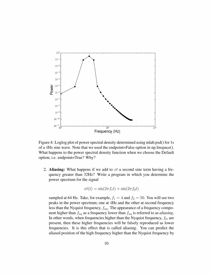
Figure 4: Loglog plot of power spectral density determined using mlab.psd() for 1sof a 4Hz sine wave. Note that we used the endpoint=False option in np.linspace().What happens to the power spectral density function when we choose the Defaultoption, i.e. endpoint=True? Why?

2. Aliasing: What happens if we add to xt a second sine term having a fre-quency greater than 32Hz? Write a program in which you determine thepower spectrum for the signal

xt(t) = sin(2πf1t) + sin(2πf2t)

sampled at 64 Hz. Take, for example, f1 = 4 and f2 = 50. You will see twopeaks in the power spectrum; one at 4Hz and the other at second frequencyless than the Nyquist frequency, fnq. The appearance of a frequency compo-nent higher than fnq as a frequency lower than fnq is referred to as aliasing.In other words, when frequencies higher than the Nyquist frequency, f0, arepresent, then these higher frequencies will be falsely reproduced as lowerfrequencies. It is this effect that is called aliasing. You can predict thealiased position of the high frequency higher than the Nyquist frequency by

10

using the relationship

sin(2π[2fNyq − f ]tn + φ) = − sin(2πf ′tn − φ) ,

where φ is the phase and t′ = 2fNyqf . Thus for example, for a compactdisk, the Nyquist frequency is fnq = 22050. Hence a signal at a frequencyof 34, 100 Hz will look exactly like a signal at a frequency of 44, 100 −34, 100 = 10, 000Hz. Use this equation to predict where the aliased sinewave peak will appear in your power spectrum?

3. The data file, sway.csv, is a two minute recording of the fluctuations inthe center of pressure (COP) for a healthy adult standing quietly on a forceplatform with eye closed. The data is sampled at 200 Hz. The first columnin the data file is the x-coordinate (medio-lateral) of the COP and the secondcolumn is the y-coordinate (anterior-posterior). Write a Python program tocalculate X =

√x2 + y2 and then determine the power spectral density

using psd(). Do you think that there is a significant periodic componentpresent?

The data file, fish_1s_10000.tsv, is 1 second of the electrical signalsgenerated by a Keck Science Department electric fish sampled at 10000 Hz.It is two columns of data: the first column is the time and the second columnis the voltage. The species of electric fish can often be determined from thepower spectrum [4]. A copy of the paper by Fugere and Kruhe on electricfish power spectra will be supplied to you in the lab. Using the results ofthis paper determine which type of electric fish corresponds to the one youcalculated the power spectrum for.

3 Exercise 2: Low-frequency signalsIn biology, we are often interested in detecting frequencies that are less than 1Hz. Examples include the resting adult respiratory rhythm (0.13−0.33Hz), circa-dian rhythms (≈ 10−5Hz), a 10-year population cycle (≈ 10−9). How do we usemlab.psd() to calculate the power spectral density of such signals?

The important question to ask is what is the minimal length of time series thatis required. Suppose we wanted to look for periodic components of 0.1Hz. A0.1Hz rhythm will have 1 cycle every 10 seconds. Thus the length of time seriesmust be at least 10 seconds long. However, we will clearly get a much better

11

looking power spectrum the longer the time series so maybe we should use 10times longer, e.g. 100s. In mlab.psd() we use the same trick as describedabove to increase the resolution, namely, we set for example NFFT=6400 andFs=64. We will return to this problem in Laboratory 11. However, you shouldverify that this procedure works for calculating the power spectral density of a 0.1Hz sine wave.

There are a number of important issues related to the characterization of theproperties of low frequency signals. The most important are related to the factthat as the frequency we wish to resolve become slower, the length of the timeseries needed to resolve the signal rapidly becomes very long. As the length ofthe required signal becomes longer, issues related to the stationarity of the signalbecome important. For example, there can be slow DC-baseline drifts in the out-puts of measurement devices, artifacts related to movement and sweating and asin the case of the EEG, biological systems tend to naturally be continuously vary-ing. Thus it is possible that a low frequency signal of interest can be lost in thenon-stationarity of the process. Another problem arises because of the prevalenceof noise in biological system which typically contributes power to the spectrumproportional to 1/f . Consequently low-frequency signals can be lost in the noise.

4 Exercise 3: FFT Applications

4.1 Convolution:Consider our black box analogy of a dynamical system. If the dynamical systemis linear then the output for any input can be determined using the convolutionintegral as

output (t) =

∫ ∞−∞

impulse (t) input (t− u)du .

If we use the Fourier transform then

Output (f) = Impulse (f) Input (f) , (2)

where the capital letters have been used to indicate the Fourier transform. Sincethe required Fourier transforms can be performed numerically using the FFT, (2)provides another method for solving the convolution integral.

However, there are practical problems using the FFT to solve the convolutionintegral. The mathematical description of the integral transforms involves timeseries that are infinitely long. On the other hand, experimentally attained time

12

series are always finite. Thus the will be effects, collectively referred to as endeffects, that effect the evaluation of the integral transform and consequently theevaluation of the convolution integral. The practical solution is to pad the timeseries with zeros [5]!

Performing the convolution integral assumes that 1) the length of the impulseresponse function is the same as the length of the input time series, and 2) theinput time series is periodic. The solution to the first problem is straight-forward:we pad the impulse response function by extending it with 0’s so that its totallength equals that of the input time series. In order to understand how the secondproblem can be dealt with it is useful to refer to the graphical interpretation ofthe convolution integral that we introduced in Laboratory 8. As a consequence offolding, displacement and multiplication, a portion of each end of the input timeseries is erroneously wrapped around by convolution with the impulse responsefunction. Thus we need to pad one end of the input time series with zeros to ensurethat the convolution integral is not contaminated from the effects of this wraparound effect. If the length of the time series is N and of the impulse function isM , then the input time series is padded at one end with N +M zeros [5].

The program used in Laboratory 7 used np.convolve() to solve the con-volution integral can be modified to use np.fft.fft() to do the same exer-cise. The program is called convolve_fft.py. We have modified this pro-gram with the lines that pad with zeros deleted. You are asked to supply themissing lines (if you can’t figure this out you can check the lines in the pro-grams convolve_fft_neuron.py or convolve_fft_sine.py on thewebsite).

4.2 Filtering imagesConvolution of an input with a linear filter in the temporal domain is equivalent tomultiplication of the Fourier transforms for the input and the filter in the frequencydomain. This provides a conceptually simple way to think about filtering: trans-form your signal into the frequency domain, dampen the frequencies that you arenot interested in by multiplying the frequency spectrum by the desired weights,and then do an inverse transform to get the filtered signal.

To illustrate consider the picture shown in the top left corner of Figure 5 wastaken by a camera attached to a robot on the surface of the moon (moonlanding.png).The picture is contaminated with high frequency noise related to the generationand transmission of the image back to earth. How can we filter away the noise sothat we can see the sharper image shown in the lower left hand corner of Figure 5?

13

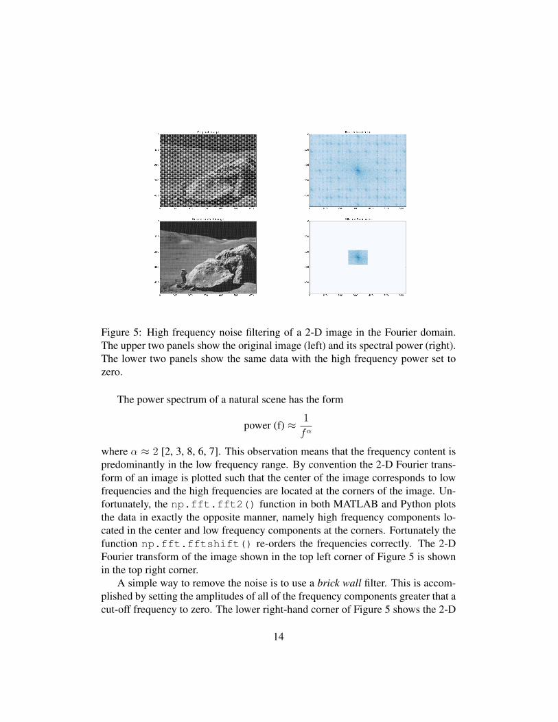
Figure 5: High frequency noise filtering of a 2-D image in the Fourier domain.The upper two panels show the original image (left) and its spectral power (right).The lower two panels show the same data with the high frequency power set tozero.

The power spectrum of a natural scene has the form

power (f) ≈ 1

fα

where α ≈ 2 [2, 3, 8, 6, 7]. This observation means that the frequency content ispredominantly in the low frequency range. By convention the 2-D Fourier trans-form of an image is plotted such that the center of the image corresponds to lowfrequencies and the high frequencies are located at the corners of the image. Un-fortunately, the np.fft.fft2() function in both MATLAB and Python plotsthe data in exactly the opposite manner, namely high frequency components lo-cated in the center and low frequency components at the corners. Fortunately thefunction np.fft.fftshift() re-orders the frequencies correctly. The 2-DFourier transform of the image shown in the top left corner of Figure 5 is shownin the top right corner.

A simple way to remove the noise is to use a brick wall filter. This is accom-plished by setting the amplitudes of all of the frequency components greater that acut-off frequency to zero. The lower right-hand corner of Figure 5 shows the 2-D

14

Fourier transform of the brick all filtered image. This is not always the best way todo this filtering: sharp edges in one domain usually introduce artifacts in another.However, it is easy to do as a first pass and sometimes provides satisfactory results(see lower left hand corner of Figure 5).

The program moon.py filters the images shown in Figure 5. As in the pre-vious example, we ask you to supply the missing lines which perform the brickwall filtering (if you can’t figure this out you can check the lines in the programconvolve_fft.py on the website.

5 SpectrogramsA spectrogram is a plot of the power spectrum as a function of time. For eachtime (indicated on the x-axis) the variance of the power spectrum as a function offrequency is plotted along the y-axis. A color or gray scale is used to indicate themagnitude of the variance. In this way a 3-D plot is plotted in 2-D.

Spectrograms are used to plot the power spectra describing the evolution of atime-varying process. Perhaps the most common uses of a spectrogram are to ana-lyze spoken words and the calls of animals, such as bird songs. Other applicationsincludes the analysis of music, sonar, radar and seismology.

Here we illustrate the use of a spectrogram by looking at a bird song. Mostoften bird songs are stored in a *.wav file. A *.wav file is the standard Microsoftaudio file format. There are several Internet sites from which *.wav files can bedownloaded for analysis, for example,

http://www.ilovewavs.com/Effects/Birds/Birds.htm

Bird songs are also recorded in mp3 format. In this case the mp3 files can beconverted to *.wav files.

There are two practical problems. First, in our experience, *.wav file down-loaded from the Internet are often corrupted. Fortunately such files can often berestored by using a software package called Audacity which can be freely down-loaded. Moreover, a useful U-tube video explains how to use Audacity to recovera corrupted *.wav file

http://www.youtube.com/watch?v=zaVr_WLikqs

The second problem is that Python currently has no audio playback software.Therefore in order to hear the birdsong you will need to use a Quick time player

15

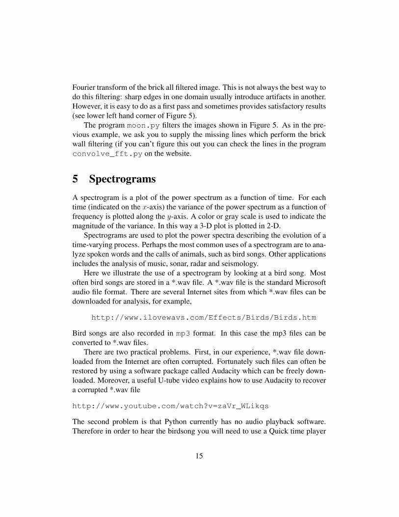
Figure 6: Spectrogram for a goldfinch.

or some other software package to hear the bird song (Windows Media Player(PCs) or Quick Time (PCs and Mac’s).

Figure 6 shows the birdsong of a goldfinch downloaded from the above birdsong website. The bird calls out twice. By looking at the spectrogram alone,can you guess what the call sounds like? The Python program that generates thisspectrogram is called spectro_bird.py. Modify this program so that thegenerated spectrogram uses a color scale instead of a gray scale.

Deliverables: Use Lab9_template.tex to prepare the lab assignment.

References[1] J. S. Bendat and A. G. Piersol. Random Data: Analysis and Measurement

Procedures, Second Edition. John Wiley & Sons, New York, 1986.

[2] D. J. Field. Rotation between the statistics of natural images and the responseproperties of cortical cells. J. Opt. Soc. Amer. A, 4:2379–2394, 1987.

[3] D. J. Field and N. Brady. Visual sensitivity, blur and the sources of variabilityin the amplitude spectra of natural scenes. Vision Res., 37:3367–3382, 1997.

16

[4] V. Fugere and R. Krahe. Electric signals and species recognition in the wave–type gymnotiform fish apteronotus leptorhynchus. J. Exp. Biol., 213:225–236,2010.

[5] W. H. Press, S. A. Teukolsky, W. T. Vetterling, and B. P. Flannery. Numericalrecipes: The art of scientific computing, third edition. Cambridge UniversityPress, New York, 2007.

[6] D. L. Ruderman. Origins of scaling in natural images. Vision Res., 37:3385–3398, 1977.

[7] D. L. Ruderman and W. Bialek. Statistics of natural images: scaling in thewoods. Phys. Rev. Lett., 73:814–817, 1994.

[8] D. J. Tolhurst, Y. Tudmor, and T. Chao. Amplitude spectra of natural images.Ophthalm. Physiol. Optics, 12:229–232, 1992.

17