Embed Size (px)
Citation preview

1
LAB MANUAL
Data Base Management Systems Lab ( CSE-212 F)
DEPARTMENT OF COMPUTER SCIENCE AND ENGINEERING
2
Check list for Lab Manual
S. No. Particulars Page
Number
1 Mission and Vision 3
2 Guidelines for the student 4
3 List of Programs as per University 5-6
4 Practical Beyond Syllabus 7
5 Sample copy of File 8-57

3
Mission
To develop BRCM College of Engineering & Technology into a “Center of Excellence”
By :
Providing State – of – the art Laboratories, Workshops, Research and instructional
facilities
Encouraging students to delve into technical pursuits beyond their academic curriculum.
Facilitating Post – graduate teaching and research
Creating an environment for complete personality development of students.
Assisting in the best possible placement
Vision
To Nurture and Harness talent for empowerment towards self actualization in all
technical domains – both existing for the future
4
Guidelines for the Students :
1. Students should be regular and come prepared for the lab practice.
2. In case a student misses a class, it is his/her responsibility to complete that missed
experiment(s).
3. Students should bring the observation book, lab journal and lab manual. Prescribed textbook
and class notes can be kept ready for reference if required.
4. They should implement the given Program individually.
5. While conducting the experiments students should see that their programs would meet the
following criteria:
Programs should be interactive with appropriate prompt messages, error messages if any,
and descriptive messages for outputs.
Programs should perform input validation (Data type, range error, etc.) and give
appropriate error messages and suggest corrective actions.
Comments should be used to give the statement of the problem and every function should
indicate the purpose of the function, inputs and outputs
Statements within the program should be properly indented
Use meaningful names for variables and functions.
Make use of Constants and type definitions wherever needed.
6. Once the experiment(s) get executed, they should show the program and results to the
instructors and copy the same in their observation book.
7. Questions for lab tests and exam need not necessarily be limited to the questions in the
manual, but could involve some variations and / or combinations of the questions.

5
Books for Reference :
Database System Concepts by A. Silberschatz, H.F. Korth and S. Sudarshan, 3rdedition, 1997, McGraw-
Hill, International Edition.
Introduction to Database Management system by Bipin Desai, 1991, Galgotia Pub.
LIST OF PROGRAMS(University Syllabus)
DBMS Lab ( CSE 212 F) Semester : IV CSE
S.NO PROGRAM
1 Create a database and write the programs to carry out the following operation:
1. Add a record in the database
2. Delete a record in the database
3. Modify the record in the database
4. Generate queries
5. Generate the report
6. List all the records of database in ascending order.
2 Develop two menu driven project for management of database system:
1. Library information system
a. Engineering
b. MCA
2. Inventory control system
a. Computer Lab
b. College Store
3. Student information system
c. Academic
d. Finance
4. Time table development system
e. CSE, IT & MCA Departments
f. Electrical & Mechanical Departments

6
Fundamentals of Database Systems by R. Elmasri and S.B. Navathe, 3 rd edition, 2000, Addision-
Wesley, Low Priced Edition.
An Introduction to Database Systems by C.J. Date, 7th
edition, Addison-Wesley, Low Priced Edition,
2000.
Database Management and Design by G.W. Hansen and J.V. Hansen, 2nd
edition,1999, Prentice-Hall of
India, Eastern Economy Edition.
Database Management Systems by A.K. Majumdar and P. Bhattacharyya, 5 th edition, 1999, Tata
McGraw-Hill Publishing.
A Guide to the SQL Standard, Date, C. and Darwen,H. 3rd edition, Reading, MA: 1994, Addison-
Wesley.

7
Practical beyond Syllabus
P.No. Program
1. Introduction to SQL
Introduction to Expressions, Conditions, and Operators
Introduction to Different Clauses in SQL
Introduction To Join : Joining Tables.
8
PROGRAM 1
AIM: Introduction to SQL
The history of SQL begins in an IBM laboratory in San Jose, California, where SQL was developed in the late
1970s. The initials stand for Structured Query Language, and the language itself is often referred to as "sequel."
It was originally developed for IBM's DB2 product (a relational database management system, or RDBMS, that
can still be bought today for various platforms and environments). In fact, SQL makes an RDBMS possible.
SQL is a nonprocedural language, in contrast to the procedural or third-generation languages (3GLs) such as
COBOL and C that had been created up to that time. The characteristic that differentiates a DBMS from an
RDBMS is that the RDBMS provides a set-oriented database language. For most RDBMSs, this set-oriented
database language is SQL. Set oriented means that SQL processes sets of data in groups.
Dr. Codd's 12 Rules for a Relational Database Model
A relational DBMS must be able to manage databases entirely through its relational capabilities.
1. Information rule-- All information in a relational database (including table and column names) is represented
explicitly as values in tables.
2. Guaranteed access--Every value in a relational database is guaranteed to be accessible by using a
combination of the table name, primary key value, and column name.
3. Systematic null value support--The DBMS provides systematic support for the treatment of null values
(unknown or inapplicable data), distinct from default values, and independent of any domain.
4. Active, online relational catalog--The description of the database and its contents is represented at the logical
level as tables and can therefore be queried using the database language.
5. Comprehensive data sublanguage--At least one supported language must have a well-defined syntax and be
comprehensive. It must support data definition, manipulation, integrity rules, authorization, and transactions.
6. View updating rule--All views that are theoretically updatable can be updated through the system.
7. Set-level insertion, update, and deletion--The DBMS supports not only set-level retrievals but also set-level
inserts, updates, and deletes.
8. Physical data independence--Application programs and ad hoc programs are logically unaffected when
physical access methods or storage structures are altered.
9. Logical data independence--Application programs and ad hoc programs are logically unaffected, to the extent
possible, when changes are made to the table structures.
10. Integrity independence--The database language must be capable of defining integrity rules. They must be
stored in the online catalog, and they cannot be bypassed.
11. Distribution independence--Application programs and ad hoc requests are logically unaffected when data is
first distributed or when it is redistributed.
12. Nonsubversion--It must not be possible to bypass the integrity rules defined through the database language
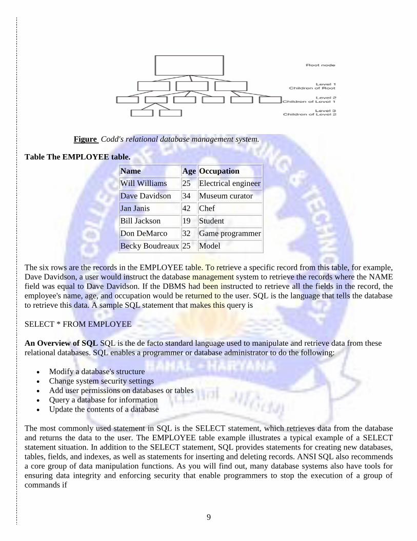
by using lower-level languages. Most databases have had a parent/child" relationship; that is, a parent node
would contain file pointers to its children.
9
Figure Codd's relational database management system.
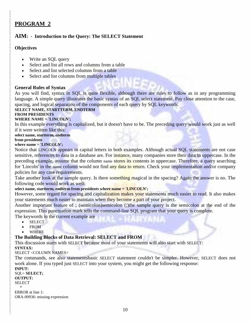
Table The EMPLOYEE table.
Name Age Occupation
Will Williams 25 Electrical engineer
Dave Davidson 34 Museum curator
Jan Janis 42 Chef
Bill Jackson 19 Student
Don DeMarco 32 Game programmer
Becky Boudreaux 25 Model
The six rows are the records in the EMPLOYEE table. To retrieve a specific record from this table, for example,
Dave Davidson, a user would instruct the database management system to retrieve the records where the NAME
field was equal to Dave Davidson. If the DBMS had been instructed to retrieve all the fields in the record, the
employee's name, age, and occupation would be returned to the user. SQL is the language that tells the database
to retrieve this data. A sample SQL statement that makes this query is
SELECT * FROM EMPLOYEE
An Overview of SQL SQL is the de facto standard language used to manipulate and retrieve data from these
relational databases. SQL enables a programmer or database administrator to do the following:
Modify a database's structure
Change system security settings
Add user permissions on databases or tables
Query a database for information
Update the contents of a database
The most commonly used statement in SQL is the SELECT statement, which retrieves data from the database
and returns the data to the user. The EMPLOYEE table example illustrates a typical example of a SELECT
statement situation. In addition to the SELECT statement, SQL provides statements for creating new databases,
tables, fields, and indexes, as well as statements for inserting and deleting records. ANSI SQL also recommends
a core group of data manipulation functions. As you will find out, many database systems also have tools for
ensuring data integrity and enforcing security that enable programmers to stop the execution of a group of
commands if
10
PROGRAM 2
AIM: - Introduction to the Query: The SELECT Statement
Objectives
Write an SQL query
Select and list all rows and columns from a table
Select and list selected columns from a table
Select and list columns from multiple tables
General Rules of Syntax
As you will find, syntax in SQL is quite flexible, although there are rules to follow as in any programming
language. A simple query illustrates the basic syntax of an SQL select statement. Pay close attention to the case,
spacing, and logical separation of the components of each query by SQL keywords. SELECT NAME, STARTTERM, ENDTERM
FROM PRESIDENTS
WHERE NAME = 'LINCOLN';
In this example everything is capitalized, but it doesn't have to be. The preceding query would work just as well
if it were written like this: select name, startterm, endterm
from presidents
where name = 'LINCOLN';
Notice that LINCOLN appears in capital letters in both examples. Although actual SQL statements are not case
sensitive, references to data in a database are. For instance, many companies store their data in uppercase. In the
preceding example, assume that the column name stores its contents in uppercase. Therefore, a query searching
for 'Lincoln' in the name column would not find any data to return. Check your implementation and/or company
policies for any case requirements.
Take another look at the sample query. Is there something magical in the spacing? Again the answer is no. The
following code would work as well: select name, startterm, endterm from presidents where name = 'LINCOLN';
However, some regard for spacing and capitalization makes your statements much easier to read. It also makes
your statements much easier to maintain when they become a part of your project.
Another important feature of ; (semicolon)semicolon (;)the sample query is the semicolon at the end of the
expression. This punctuation mark tells the command-line SQL program that your query is complete.
The keywords in the current example are SELECT FROM WHERE
The Building Blocks of Data Retrieval: SELECT and FROM
This discussion starts with SELECT because most of your statements will also start with SELECT: SYNTAX:
SELECT <COLUMN NAMES>
The commands, see also statementsbasic SELECT statement couldn't be simpler. However, SELECT does not
work alone. If you typed just SELECT into your system, you might get the following response: INPUT:
SQL> SELECT;
OUTPUT:
SELECT
*
ERROR at line 1:
ORA-00936: missing expression
11
The asterisk under the offending line indicates where Oracle7 thinks the offense occurred. The error message
tells you that something is missing. That something is the FROM clause: SYNTAX:
FROM <TABLE>
Together, the statements SELECT and FROM begin to unlock the power behind your database.
Examples
Before going any further, look at the sample database that is the basis for the following examples. This database
illustrates the basic functions of SELECT and FROM. In the real world you would use the techniques described on
Day 8, "Manipulating Data," to build this database, but for the purpose of describing how to use SELECT and
FROM, assume it already exists. This example uses the CHECKS table to retrieve information about checks that
an individual has written.
The CHECKS table: CHECK# PAYEE AMOUNT REMARKS
--------- -------------------- ------ ---------------------
1 Ma Bell 150 Have sons next time
2 Reading R.R. 245.34 Train to Chicago
3 Ma Bell 200.32 Cellular Phone
4 Local Utilities 98 Gas
5 Joes Stale $ Dent 150 Groceries
6 Cash 25 Wild Night Out
7 Joans Gas 25.1 Gas
Your First Query INPUT:
SQL> select * from checks;
OUTPUT:
queriesCHECK# PAYEE AMOUNT REMARKS
------ -------------------- ------- ---------------------
1 Ma Bell 150 Have sons next time
2 Reading R.R. 245.34 Train to Chicago
3 Ma Bell 200.32 Cellular Phone
4 Local Utilities 98 Gas
5 Joes Stale $ Dent 150 Groceries
6 Cash 25 Wild Night Out
7 Joans Gas 25.1 Gas
7 rows selected.
ANALYSIS:
This output looks just like the code in the example. Notice that columns 1 and 3 in the output statement are
right-justified and that columns 2 and 4 are left-justified. This format follows the alignment convention in
which numeric data types are right-justified and character data types are left-justified. Data types are discussed
on Day 9, "Creating and Maintaining Tables."
The asterisk (*) in select * tells the database to return all the columns associated with the given table described in
the FROM clause. The database determines the order in which to return the columns.
Terminating an SQL Statement
In some implementations of SQL, the semicolon at the end of the statement tells the interpreter that you are
finished writing the query. For example, Oracle's SQL*PLUS won't execute the query until it finds a semicolon
(or a slash). On the other hand, some implementations of SQL do not use the semicolon as a terminator. For
example, Microsoft Query and Borland's ISQL don't require a terminator, because your query is typed in an edit
box and executed when you push a button.
Changing the Order of the Columns
The preceding example of an SQL statement used the * to select all columns from a table, the order of their
appearance in the output being determined by the database. To specify the order of the columns, you could type
something like: INPUT:
SQL> SELECT payee, remarks, amount, check# from checks;
12
Notice that each column name is listed in the SELECT clause. The order in which the columns are listed is the
order in which they will appear in the output. Notice both the commas that separate the column names and the
space between the final column name and the subsequent clause (in this case FROM). The output would look like
this: OUTPUT:
PAYEE REMARKS AMOUNT CHECK#
-------------------- ------------------ --------- ---------
Ma Bell Have sons next time 150 1
Reading R.R. Train to Chicago 245.34 2
Ma Bell Cellular Phone 200.32 3
Local Utilities Gas 98 4
Joes Stale $ Dent Groceries 150 5
Cash Wild Night Out 25 6
Joans Gas Gas 25.1 7
7 rows selected.
Another way to write the same statement follows. INPUT:
SELECT payee, remarks, amount, check#
FROM checks;
Notice that the FROM clause has been carried over to the second line. This convention is a matter of personal
taste when writing SQL code. The output would look like this: OUTPUT:
PAYEE REMARKS AMOUNT CHECK#
-------------------- -------------------- --------- --------
Ma Bell Have sons next time 150 1
Reading R.R. Train to Chicago 245.34 2
Ma Bell Cellular Phone 200.32 3
Local Utilities Gas 98 4
Joes Stale $ Dent Groceries 150 5
Cash Wild Night Out 25 6
Joans Gas Gas 25.1 7
7 rows selected.
ANALYSIS:
The output is identical because only the format of the statement changed. Now that you have established control
over the order of the columns, you will be able to specify which columns you want to see.
Selecting Individual Columns
Suppose you do not want to see every column in the database. You used SELECT * to find out what information
was available, and now you want to concentrate on the check number and the amount. You type INPUT:
SQL> SELECT CHECK#, amount from checks;
which returns OUTPUT:
CHECK# AMOUNT
--------- ---------
1 150
2 245.34
3 200.32
4 98
5 150
6 25
7 25.1
7 rows selected.
ANALYSIS:
13
Now you have the columns you want to see. Notice the use of upper- and lowercase in the query. It did not
affect the result.
What if you need information from a different table?
Selecting Different Tables
Suppose you had a table called DEPOSITS with this structure: DEPOSIT# WHOPAID AMOUNT REMARKS
-------- ---------------------- ------ -------------------
1 Rich Uncle 200 Take off Xmas list
2 Employer 1000 15 June Payday
3 Credit Union 500 Loan
You would simply change the FROM clause to the desired table and type the following statement: INPUT:
SQL> select * from deposits
The result is OUTPUT:
DEPOSIT# WHOPAID AMOUNT REMARKS
-------- ---------------------- ------ -------------------
1 Rich Uncle 200 Take off Xmas list
2 Employer 1000 15 June Payday
3 Credit Union 500 Loan
ANALYSIS:
With a single change you have a new data source.
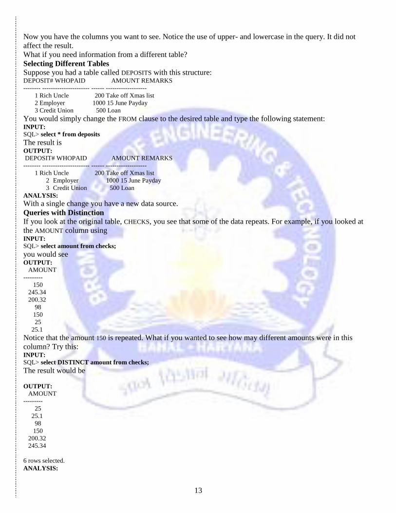
Queries with Distinction
If you look at the original table, CHECKS, you see that some of the data repeats. For example, if you looked at
the AMOUNT column using INPUT:
SQL> select amount from checks;
you would see OUTPUT:
AMOUNT
---------
150
245.34
200.32
98
150
25
25.1
Notice that the amount 150 is repeated. What if you wanted to see how may different amounts were in this
column? Try this: INPUT:
SQL> select DISTINCT amount from checks;
The result would be
OUTPUT:
AMOUNT
---------
25
25.1
98
150
200.32
245.34
6 rows selected.
ANALYSIS:
14
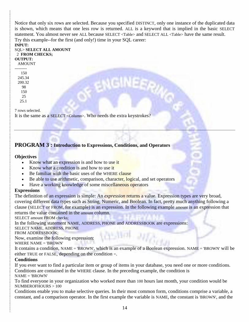
Notice that only six rows are selected. Because you specified DISTINCT, only one instance of the duplicated data
is shown, which means that one less row is returned. ALL is a keyword that is implied in the basic SELECT
statement. You almost never see ALL because SELECT <Table> and SELECT ALL <Table> have the same result.
Try this example--for the first (and only!) time in your SQL career: INPUT:
SQL> SELECT ALL AMOUNT
2 FROM CHECKS;
OUTPUT:
AMOUNT
---------
150
245.34
200.32
98
150
25
25.1
7 rows selected.
It is the same as a SELECT <Column>. Who needs the extra keystrokes?
PROGRAM 3 : Introduction to Expressions, Conditions, and Operators
Objectives
Know what an expression is and how to use it
Know what a condition is and how to use it
Be familiar with the basic uses of the WHERE clause
Be able to use arithmetic, comparison, character, logical, and set operators
Have a working knowledge of some miscellaneous operators
Expressions
The definition of an expression is simple: An expression returns a value. Expression types are very broad,
covering different data types such as String, Numeric, and Boolean. In fact, pretty much anything following a
clause (SELECT or FROM, for example) is an expression. In the following example amount is an expression that
returns the value contained in the amount column. SELECT amount FROM checks;
In the following statement NAME, ADDRESS, PHONE and ADDRESSBOOK are expressions: SELECT NAME, ADDRESS, PHONE
FROM ADDRESSBOOK;
Now, examine the following expression: WHERE NAME = 'BROWN'
It contains a condition, NAME = 'BROWN', which is an example of a Boolean expression. NAME = 'BROWN' will be
either TRUE or FALSE, depending on the condition =.
Conditions
If you ever want to find a particular item or group of items in your database, you need one or more conditions.
Conditions are contained in the WHERE clause. In the preceding example, the condition is NAME = 'BROWN'
To find everyone in your organization who worked more than 100 hours last month, your condition would be NUMBEROFHOURS > 100
Conditions enable you to make selective queries. In their most common form, conditions comprise a variable, a
constant, and a comparison operator. In the first example the variable is NAME, the constant is 'BROWN', and the
15
comparison operator is =. In the second example the variable is NUMBEROFHOURS, the constant is 100, and the
comparison operator is >. You need to know about two more elements before you can write conditional queries:
the WHERE clause and operators.
The WHERE Clause
The syntax of the WHERE clause is SYNTAX:
WHERE <SEARCH CONDITION>
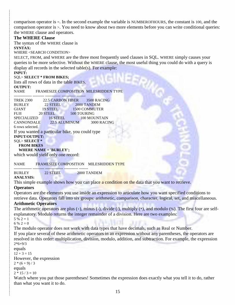
SELECT, FROM, and WHERE are the three most frequently used clauses in SQL. WHERE simply causes your
queries to be more selective. Without the WHERE clause, the most useful thing you could do with a query is
display all records in the selected table(s). For example: INPUT:
SQL> SELECT * FROM BIKES;
lists all rows of data in the table BIKES. OUTPUT:
NAME FRAMESIZE COMPOSITION MILESRIDDEN TYPE
-------------- --------- ------------ ----------- -------
TREK 2300 22.5 CARBON FIBER 3500 RACING
BURLEY 22 STEEL 2000 TANDEM
GIANT 19 STEEL 1500 COMMUTER
FUJI 20 STEEL 500 TOURING
SPECIALIZED 16 STEEL 100 MOUNTAIN
CANNONDALE 22.5 ALUMINUM 3000 RACING
6 rows selected.
If you wanted a particular bike, you could type INPUT/OUTPUT:
SQL> SELECT *
FROM BIKES
WHERE NAME = 'BURLEY';
which would yield only one record:
NAME FRAMESIZE COMPOSITION MILESRIDDEN TYPE
-------------- --------- -------------- ----------- -------
BURLEY 22 STEEL 2000 TANDEM
ANALYSIS:
This simple example shows how you can place a condition on the data that you want to retrieve.
Operators
Operators are the elements you use inside an expression to articulate how you want specified conditions to
retrieve data. Operators fall into six groups: arithmetic, comparison, character, logical, set, and miscellaneous.
Arithmetic Operators
The arithmetic operators are plus (+), minus (-), divide (/), multiply (*), and modulo (%). The first four are self-
explanatory. Modulo returns the integer remainder of a division. Here are two examples: 5 % 2 = 1
6 % 2 = 0
The modulo operator does not work with data types that have decimals, such as Real or Number.
If you place several of these arithmetic operators in an expression without any parentheses, the operators are
resolved in this order: multiplication, division, modulo, addition, and subtraction. For example, the expression 2*6+9/3
equals 12 + 3 = 15
However, the expression 2 * (6 + 9) / 3
equals 2 * 15 / 3 = 10
Watch where you put those parentheses! Sometimes the expression does exactly what you tell it to do, rather
than what you want it to do.

16
The following sections examine the arithmetic operators in some detail and give you a chance to write some
queries.
Plus (+)
You can use the plus sign in several ways. Type the following statement to display the PRICE table: INPUT:
SQL> SELECT * FROM PRICE;
OUTPUT:
ITEM WHOLESALE
-------------- ----------
TOMATOES .34
POTATOES .51
BANANAS .67
TURNIPS .45
CHEESE .89
APPLES .23
6 rows selected.
Now type: INPUT/OUTPUT:
SQL> SELECT ITEM, WHOLESALE, WHOLESALE + 0.15
FROM PRICE;
Here the + adds 15 cents to each price to produce the following: ITEM WHOLESALE WHOLESALE+0.15
-------------- --------- --------------
TOMATOES .34 .49
POTATOES .51 .66
BANANAS .67 .82
TURNIPS .45 .60
CHEESE .89 1.04
APPLES .23 .38
6 rows selected.
ANALYSIS:
What is this last column with the unattractive column heading WHOLESALE+0.15? It's not in the original table.
(Remember, you used * in the SELECT clause, which causes all the columns to be shown.) SQL allows you to
create a virtual or derived column by combining or modifying existing columns.
Retype the original entry: INPUT/OUTPUT:
SQL> SELECT * FROM PRICE;
The following table results: ITEM WHOLESALE
-------------- ---------
TOMATOES .34
POTATOES .51
BANANAS .67
TURNIPS .45
CHEESE .89
APPLES .23
6 rows selected.
ANALYSIS:
The output confirms that the original data has not been changed and that the column heading WHOLESALE+0.15
is not a permanent part of it. In fact, the column heading is so unattractive that you should do something about
it.
Type the following: INPUT/OUTPUT:
SQL> SELECT ITEM, WHOLESALE, (WHOLESALE + 0.15) RETAIL
FROM PRICE;
Here's the result: ITEM WHOLESALE RETAIL
17
-------------- --------- ------
TOMATOES .34 .49
POTATOES .51 .66
BANANAS .67 .82
TURNIPS .45 .60
CHEESE .89 1.04
APPLES .23 .38
6 rows selected.
ANALYSIS:
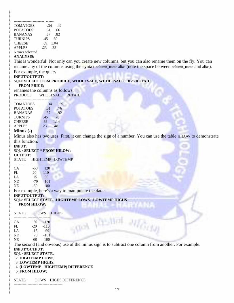
This is wonderful! Not only can you create new columns, but you can also rename them on the fly. You can
rename any of the columns using the syntax column_name alias (note the space between column_name and alias).
For example, the query INPUT/OUTPUT:
SQL> SELECT ITEM PRODUCE, WHOLESALE, WHOLESALE + 0.25 RETAIL
FROM PRICE;
renames the columns as follows: PRODUCE WHOLESALE RETAIL
-------------- --------- ---------
TOMATOES .34 .59
POTATOES .51 .76
BANANAS .67 .92
TURNIPS .45 .70
CHEESE .89 1.14
APPLES .23 .48
Minus (-)
Minus also has two uses. First, it can change the sign of a number. You can use the table HILOW to demonstrate
this function. INPUT:
SQL> SELECT * FROM HILOW;
OUTPUT:
STATE HIGHTEMP LOWTEMP
---------- -------- ---------
CA -50 120
FL 20 110
LA 15 99
ND -70 101
NE -60 100
For example, here's a way to manipulate the data: INPUT/OUTPUT:
SQL> SELECT STATE, -HIGHTEMP LOWS, -LOWTEMP HIGHS
FROM HILOW;
STATE LOWS HIGHS
---------- -------- ---------
CA 50 -120
FL -20 -110
LA -15 -99
ND 70 -101
NE 60 -100
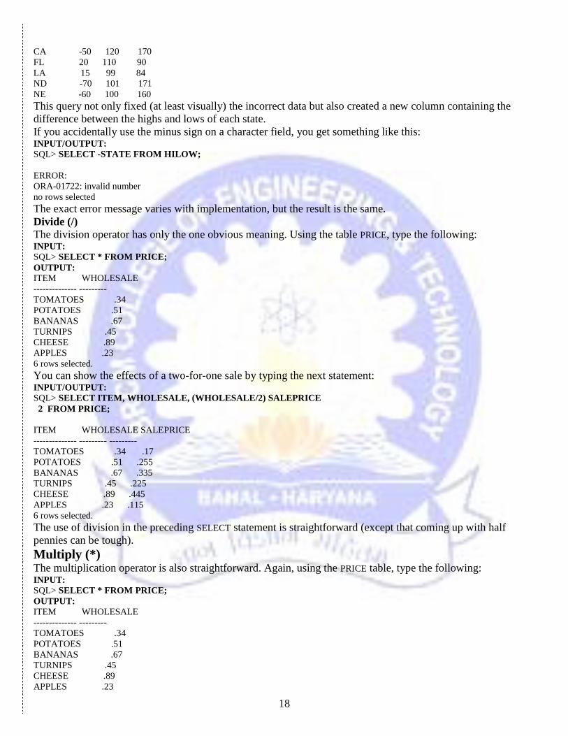
The second (and obvious) use of the minus sign is to subtract one column from another. For example: INPUT/OUTPUT:
SQL> SELECT STATE,
2 HIGHTEMP LOWS,
3 LOWTEMP HIGHS,
4 (LOWTEMP - HIGHTEMP) DIFFERENCE
5 FROM HILOW;
STATE LOWS HIGHS DIFFERENCE
---------- -------- -------- ----------
18
CA -50 120 170
FL 20 110 90
LA 15 99 84
ND -70 101 171
NE -60 100 160
This query not only fixed (at least visually) the incorrect data but also created a new column containing the
difference between the highs and lows of each state.
If you accidentally use the minus sign on a character field, you get something like this: INPUT/OUTPUT:
SQL> SELECT -STATE FROM HILOW;
ERROR:
ORA-01722: invalid number
no rows selected
The exact error message varies with implementation, but the result is the same.
Divide (/)
The division operator has only the one obvious meaning. Using the table PRICE, type the following: INPUT:
SQL> SELECT * FROM PRICE;
OUTPUT:
ITEM WHOLESALE
-------------- ---------
TOMATOES .34
POTATOES .51
BANANAS .67
TURNIPS .45
CHEESE .89
APPLES .23
6 rows selected.
You can show the effects of a two-for-one sale by typing the next statement: INPUT/OUTPUT:
SQL> SELECT ITEM, WHOLESALE, (WHOLESALE/2) SALEPRICE
2 FROM PRICE;
ITEM WHOLESALE SALEPRICE
-------------- --------- ---------
TOMATOES .34 .17
POTATOES .51 .255
BANANAS .67 .335
TURNIPS .45 .225
CHEESE .89 .445
APPLES .23 .115
6 rows selected.
The use of division in the preceding SELECT statement is straightforward (except that coming up with half
pennies can be tough).
Multiply (*) The multiplication operator is also straightforward. Again, using the PRICE table, type the following: INPUT:
SQL> SELECT * FROM PRICE;
OUTPUT:
ITEM WHOLESALE
-------------- ---------
TOMATOES .34
POTATOES .51
BANANAS .67
TURNIPS .45
CHEESE .89
APPLES .23
19
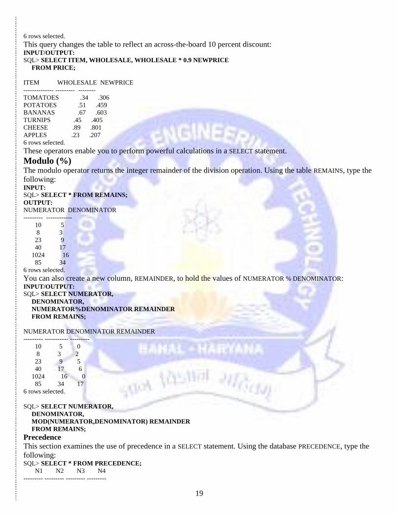
6 rows selected.
This query changes the table to reflect an across-the-board 10 percent discount: INPUT/OUTPUT:
SQL> SELECT ITEM, WHOLESALE, WHOLESALE * 0.9 NEWPRICE
FROM PRICE;
ITEM WHOLESALE NEWPRICE
-------------- --------- --------
TOMATOES .34 .306
POTATOES .51 .459
BANANAS .67 .603
TURNIPS .45 .405
CHEESE .89 .801
APPLES .23 .207
6 rows selected.
These operators enable you to perform powerful calculations in a SELECT statement.
Modulo (%) The modulo operator returns the integer remainder of the division operation. Using the table REMAINS, type the
following: INPUT:
SQL> SELECT * FROM REMAINS;
OUTPUT:
NUMERATOR DENOMINATOR
--------- ------------
10 5
8 3
23 9
40 17
1024 16
85 34
6 rows selected.
You can also create a new column, REMAINDER, to hold the values of NUMERATOR % DENOMINATOR: INPUT/OUTPUT:
SQL> SELECT NUMERATOR,
DENOMINATOR,
NUMERATOR%DENOMINATOR REMAINDER
FROM REMAINS;
NUMERATOR DENOMINATOR REMAINDER
--------- ----------- ---------
10 5 0
8 3 2
23 9 5
40 17 6
1024 16 0
85 34 17
6 rows selected.
SQL> SELECT NUMERATOR,
DENOMINATOR,
MOD(NUMERATOR,DENOMINATOR) REMAINDER
FROM REMAINS;
Precedence
This section examines the use of precedence in a SELECT statement. Using the database PRECEDENCE, type the
following: SQL> SELECT * FROM PRECEDENCE;
N1 N2 N3 N4
--------- --------- --------- ---------
20
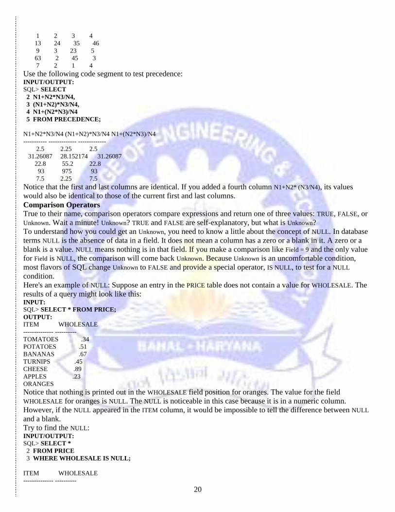
1 2 3 4
13 24 35 46
9 3 23 5
63 2 45 3
7 2 1 4
Use the following code segment to test precedence: INPUT/OUTPUT:
SQL> SELECT
2 N1+N2*N3/N4,
3 (N1+N2)*N3/N4,
4 N1+(N2*N3)/N4
5 FROM PRECEDENCE;
N1+N2*N3/N4 (N1+N2)*N3/N4 N1+(N2*N3)/N4
----------- ------------- -------------
2.5 2.25 2.5
31.26087 28.152174 31.26087
22.8 55.2 22.8
93 975 93
7.5 2.25 7.5
Notice that the first and last columns are identical. If you added a fourth column N1+N2* (N3/N4), its values
would also be identical to those of the current first and last columns.
Comparison Operators
True to their name, comparison operators compare expressions and return one of three values: TRUE, FALSE, or
Unknown. Wait a minute! Unknown? TRUE and FALSE are self-explanatory, but what is Unknown?
To understand how you could get an Unknown, you need to know a little about the concept of NULL. In database
terms NULL is the absence of data in a field. It does not mean a column has a zero or a blank in it. A zero or a
blank is a value. NULL means nothing is in that field. If you make a comparison like Field = 9 and the only value
for Field is NULL, the comparison will come back Unknown. Because Unknown is an uncomfortable condition,
most flavors of SQL change Unknown to FALSE and provide a special operator, IS NULL, to test for a NULL
condition.
Here's an example of NULL: Suppose an entry in the PRICE table does not contain a value for WHOLESALE. The
results of a query might look like this: INPUT:
SQL> SELECT * FROM PRICE;
OUTPUT:
ITEM WHOLESALE
-------------- ----------
TOMATOES .34
POTATOES .51
BANANAS .67
TURNIPS .45
CHEESE .89
APPLES .23
ORANGES
Notice that nothing is printed out in the WHOLESALE field position for oranges. The value for the field
WHOLESALE for oranges is NULL. The NULL is noticeable in this case because it is in a numeric column.
However, if the NULL appeared in the ITEM column, it would be impossible to tell the difference between NULL
and a blank.
Try to find the NULL: INPUT/OUTPUT:
SQL> SELECT *
2 FROM PRICE
3 WHERE WHOLESALE IS NULL;
ITEM WHOLESALE
-------------- ----------
21
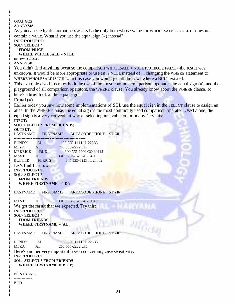
ORANGES
ANALYSIS:
As you can see by the output, ORANGES is the only item whose value for WHOLESALE is NULL or does not
contain a value. What if you use the equal sign (=) instead? INPUT/OUTPUT:
SQL> SELECT *
FROM PRICE
WHERE WHOLESALE = NULL; no rows selected
ANALYSIS:
You didn't find anything because the comparison WHOLESALE = NULL returned a FALSE--the result was
unknown. It would be more appropriate to use an IS NULL instead of =, changing the WHERE statement to
WHERE WHOLESALE IS NULL. In this case you would get all the rows where a NULL existed.
This example also illustrates both the use of the most common comparison operator, the equal sign (=), and the
playground of all comparison operators, the WHERE clause. You already know about the WHERE clause, so
here's a brief look at the equal sign.
Equal (=)
Earlier today you saw how some implementations of SQL use the equal sign in the SELECT clause to assign an
alias. In the WHERE clause, the equal sign is the most commonly used comparison operator. Used alone, the
equal sign is a very convenient way of selecting one value out of many. Try this: INPUT:
SQL> SELECT * FROM FRIENDS;
OUTPUT:
LASTNAME FIRSTNAME AREACODE PHONE ST ZIP
-------------- -------------- --------- -------- -- -----
BUNDY AL 100 555-1111 IL 22333
MEZA AL 200 555-2222 UK
MERRICK BUD 300 555-6666 CO 80212
MAST JD 381 555-6767 LA 23456
BULHER FERRIS 345 555-3223 IL 23332
Let's find JD's row. INPUT/OUTPUT:
SQL> SELECT *
FROM FRIENDS
WHERE FIRSTNAME = 'JD';
LASTNAME FIRSTNAME AREACODE PHONE ST ZIP
-------------- -------------- --------- -------- -- -----
MAST JD 381 555-6767 LA 23456
We got the result that we expected. Try this: INPUT/OUTPUT:
SQL> SELECT *
FROM FRIENDS
WHERE FIRSTNAME = 'AL';
LASTNAME FIRSTNAME AREACODE PHONE ST ZIP
-------------- -------------- --------- -------- -- -----
BUNDY AL 100 555-1111 IL 22333
MEZA AL 200 555-2222 UK
Here's another very important lesson concerning case sensitivity: INPUT/OUTPUT:
SQL> SELECT * FROM FRIENDS
WHERE FIRSTNAME = 'BUD';
FIRSTNAME
--------------
BUD
22
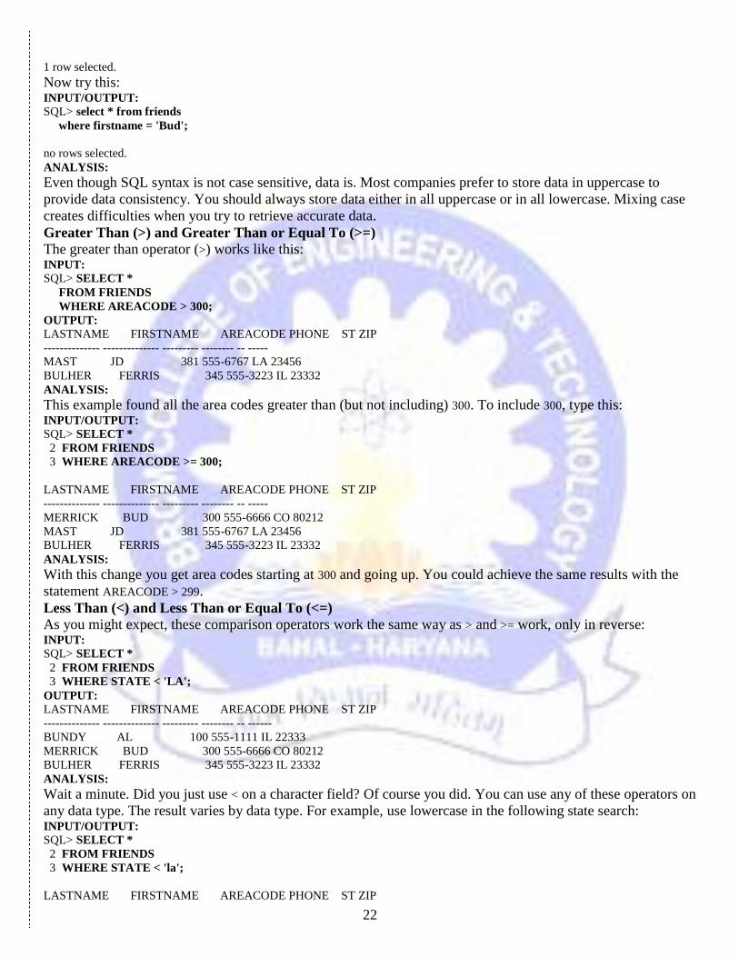
1 row selected.
Now try this: INPUT/OUTPUT:
SQL> select * from friends
where firstname = 'Bud';
no rows selected.
ANALYSIS:
Even though SQL syntax is not case sensitive, data is. Most companies prefer to store data in uppercase to
provide data consistency. You should always store data either in all uppercase or in all lowercase. Mixing case
creates difficulties when you try to retrieve accurate data.
Greater Than (>) and Greater Than or Equal To (>=)
The greater than operator (>) works like this: INPUT:
SQL> SELECT *
FROM FRIENDS
WHERE AREACODE > 300;
OUTPUT:
LASTNAME FIRSTNAME AREACODE PHONE ST ZIP
-------------- -------------- --------- -------- -- -----
MAST JD 381 555-6767 LA 23456
BULHER FERRIS 345 555-3223 IL 23332
ANALYSIS:
This example found all the area codes greater than (but not including) 300. To include 300, type this: INPUT/OUTPUT:
SQL> SELECT *
2 FROM FRIENDS
3 WHERE AREACODE >= 300;
LASTNAME FIRSTNAME AREACODE PHONE ST ZIP
-------------- -------------- --------- -------- -- -----
MERRICK BUD 300 555-6666 CO 80212
MAST JD 381 555-6767 LA 23456
BULHER FERRIS 345 555-3223 IL 23332
ANALYSIS:
With this change you get area codes starting at 300 and going up. You could achieve the same results with the
statement AREACODE > 299.
Less Than (<) and Less Than or Equal To (<=)
As you might expect, these comparison operators work the same way as > and >= work, only in reverse: INPUT:
SQL> SELECT *
2 FROM FRIENDS
3 WHERE STATE < 'LA';
OUTPUT:
LASTNAME FIRSTNAME AREACODE PHONE ST ZIP
-------------- -------------- --------- -------- -- ------
BUNDY AL 100 555-1111 IL 22333
MERRICK BUD 300 555-6666 CO 80212
BULHER FERRIS 345 555-3223 IL 23332
ANALYSIS:
Wait a minute. Did you just use < on a character field? Of course you did. You can use any of these operators on
any data type. The result varies by data type. For example, use lowercase in the following state search: INPUT/OUTPUT:
SQL> SELECT *
2 FROM FRIENDS
3 WHERE STATE < 'la';
LASTNAME FIRSTNAME AREACODE PHONE ST ZIP
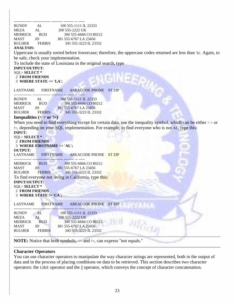
23
-------------- -------------- --------- -------- -- -----
BUNDY AL 100 555-1111 IL 22333
MEZA AL 200 555-2222 UK
MERRICK BUD 300 555-6666 CO 80212
MAST JD 381 555-6767 LA 23456
BULHER FERRIS 345 555-3223 IL 23332
ANALYSIS:
Uppercase is usually sorted before lowercase; therefore, the uppercase codes returned are less than 'la'. Again, to
be safe, check your implementation.
To include the state of Louisiana in the original search, type INPUT/OUTPUT:
SQL> SELECT *
2 FROM FRIENDS
3 WHERE STATE <= 'LA';
LASTNAME FIRSTNAME AREACODE PHONE ST ZIP
-------------- -------------- --------- -------- -- -----
BUNDY AL 100 555-1111 IL 22333
MERRICK BUD 300 555-6666 CO 80212
MAST JD 381 555-6767 LA 23456
BULHER FERRIS 345 555-3223 IL 23332
Inequalities (< > or !=)
When you need to find everything except for certain data, use the inequality symbol, which can be either < > or
!=, depending on your SQL implementation. For example, to find everyone who is not AL, type this: INPUT:
SQL> SELECT *
2 FROM FRIENDS
3 WHERE FIRSTNAME <> 'AL';
OUTPUT:
LASTNAME FIRSTNAME AREACODE PHONE ST ZIP
-------------- -------------- --------- -------- -- -----
MERRICK BUD 300 555-6666 CO 80212
MAST JD 381 555-6767 LA 23456
BULHER FERRIS 345 555-3223 IL 23332
To find everyone not living in California, type this: INPUT/OUTPUT:
SQL> SELECT *
2 FROM FRIENDS
3 WHERE STATE != 'CA';
LASTNAME FIRSTNAME AREACODE PHONE ST ZIP
-------------- -------------- --------- -------- -- -----
BUNDY AL 100 555-1111 IL 22333
MEZA AL 200 555-2222 UK
MERRICK BUD 300 555-6666 CO 80212
MAST JD 381 555-6767 LA 23456
BULHER FERRIS 345 555-3223 IL 23332
NOTE: Notice that both symbols, <> and !=, can express "not equals."
Character Operators
You can use character operators to manipulate the way character strings are represented, both in the output of
data and in the process of placing conditions on data to be retrieved. This section describes two character
operators: the LIKE operator and the || operator, which conveys the concept of character concatenation.
24
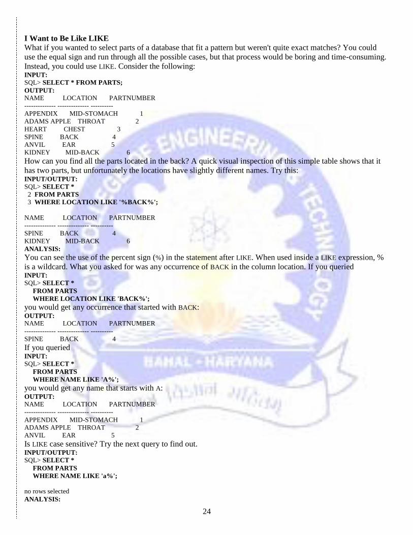
I Want to Be Like LIKE
What if you wanted to select parts of a database that fit a pattern but weren't quite exact matches? You could
use the equal sign and run through all the possible cases, but that process would be boring and time-consuming.
Instead, you could use LIKE. Consider the following: INPUT:
SQL> SELECT * FROM PARTS;
OUTPUT:
NAME LOCATION PARTNUMBER
-------------- -------------- ----------
APPENDIX MID-STOMACH 1
ADAMS APPLE THROAT 2
HEART CHEST 3
SPINE BACK 4
ANVIL EAR 5
KIDNEY MID-BACK 6
How can you find all the parts located in the back? A quick visual inspection of this simple table shows that it
has two parts, but unfortunately the locations have slightly different names. Try this: INPUT/OUTPUT:
SQL> SELECT *
2 FROM PARTS
3 WHERE LOCATION LIKE '%BACK%';
NAME LOCATION PARTNUMBER
-------------- -------------- ----------
SPINE BACK 4
KIDNEY MID-BACK 6
ANALYSIS:
You can see the use of the percent sign (%) in the statement after LIKE. When used inside a LIKE expression, %
is a wildcard. What you asked for was any occurrence of BACK in the column location. If you queried INPUT:
SQL> SELECT *
FROM PARTS
WHERE LOCATION LIKE 'BACK%';
you would get any occurrence that started with BACK: OUTPUT:
NAME LOCATION PARTNUMBER
-------------- -------------- ----------
SPINE BACK 4
If you queried INPUT:
SQL> SELECT *
FROM PARTS
WHERE NAME LIKE 'A%';
you would get any name that starts with A: OUTPUT:
NAME LOCATION PARTNUMBER
-------------- -------------- ----------
APPENDIX MID-STOMACH 1
ADAMS APPLE THROAT 2
ANVIL EAR 5
Is LIKE case sensitive? Try the next query to find out. INPUT/OUTPUT:
SQL> SELECT *
FROM PARTS
WHERE NAME LIKE 'a%';
no rows selected
ANALYSIS:
25
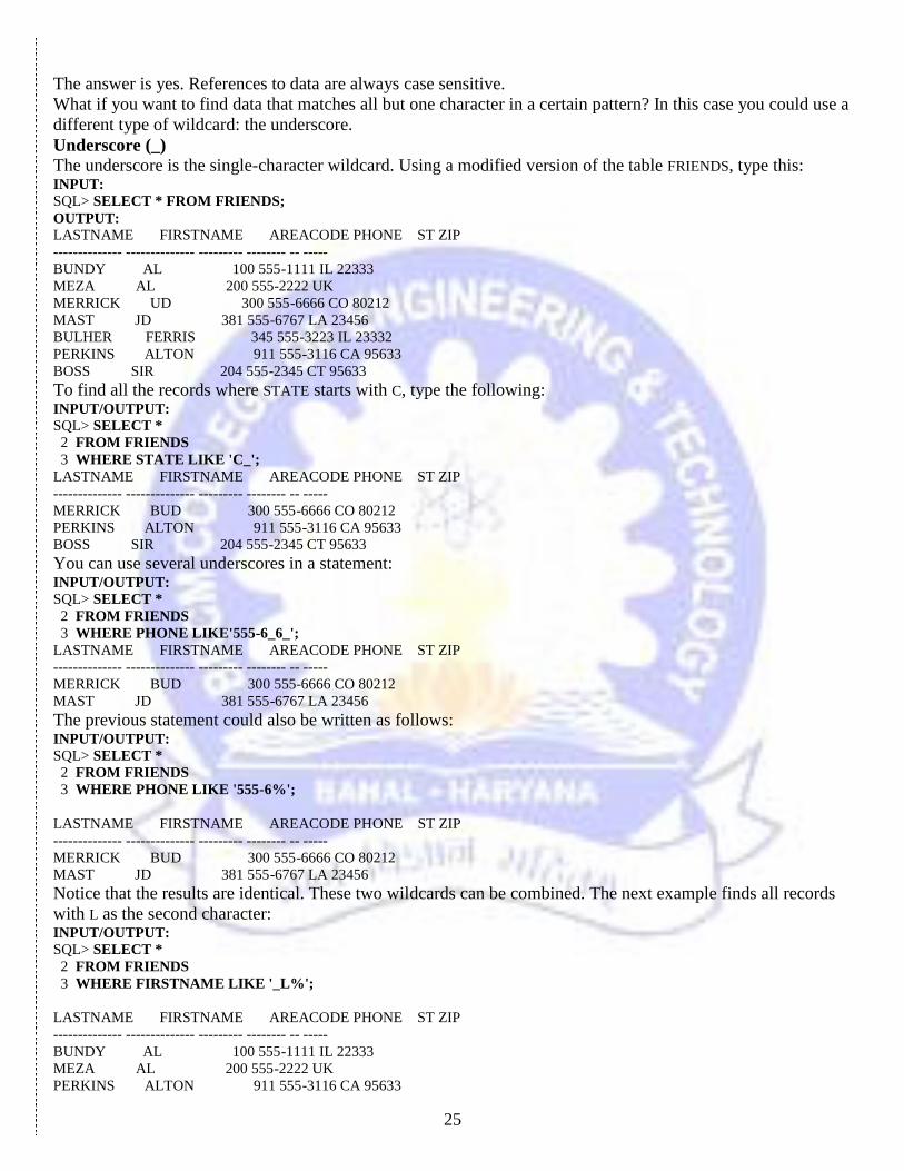
The answer is yes. References to data are always case sensitive.
What if you want to find data that matches all but one character in a certain pattern? In this case you could use a
different type of wildcard: the underscore.
Underscore (_)
The underscore is the single-character wildcard. Using a modified version of the table FRIENDS, type this: INPUT:
SQL> SELECT * FROM FRIENDS;
OUTPUT:
LASTNAME FIRSTNAME AREACODE PHONE ST ZIP
-------------- -------------- --------- -------- -- -----
BUNDY AL 100 555-1111 IL 22333
MEZA AL 200 555-2222 UK
MERRICK UD 300 555-6666 CO 80212
MAST JD 381 555-6767 LA 23456
BULHER FERRIS 345 555-3223 IL 23332
PERKINS ALTON 911 555-3116 CA 95633
BOSS SIR 204 555-2345 CT 95633
To find all the records where STATE starts with C, type the following: INPUT/OUTPUT:
SQL> SELECT *
2 FROM FRIENDS
3 WHERE STATE LIKE 'C_';
LASTNAME FIRSTNAME AREACODE PHONE ST ZIP
-------------- -------------- --------- -------- -- -----
MERRICK BUD 300 555-6666 CO 80212
PERKINS ALTON 911 555-3116 CA 95633
BOSS SIR 204 555-2345 CT 95633
You can use several underscores in a statement: INPUT/OUTPUT:
SQL> SELECT *
2 FROM FRIENDS
3 WHERE PHONE LIKE'555-6_6_';
LASTNAME FIRSTNAME AREACODE PHONE ST ZIP
-------------- -------------- --------- -------- -- -----
MERRICK BUD 300 555-6666 CO 80212
MAST JD 381 555-6767 LA 23456
The previous statement could also be written as follows: INPUT/OUTPUT:
SQL> SELECT *
2 FROM FRIENDS
3 WHERE PHONE LIKE '555-6%';
LASTNAME FIRSTNAME AREACODE PHONE ST ZIP
-------------- -------------- --------- -------- -- -----
MERRICK BUD 300 555-6666 CO 80212
MAST JD 381 555-6767 LA 23456
Notice that the results are identical. These two wildcards can be combined. The next example finds all records
with L as the second character: INPUT/OUTPUT:
SQL> SELECT *
2 FROM FRIENDS
3 WHERE FIRSTNAME LIKE '_L%';
LASTNAME FIRSTNAME AREACODE PHONE ST ZIP
-------------- -------------- --------- -------- -- -----
BUNDY AL 100 555-1111 IL 22333
MEZA AL 200 555-2222 UK
PERKINS ALTON 911 555-3116 CA 95633
26
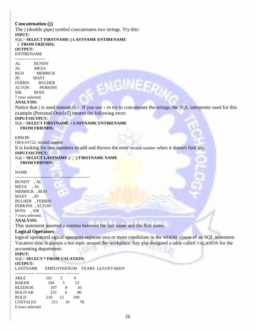
Concatenation (||)
The || (double pipe) symbol concatenates two strings. Try this: INPUT:
SQL> SELECT FIRSTNAME || LASTNAME ENTIRENAME
2 FROM FRIENDS;
OUTPUT:
ENTIRENAME
----------------------
AL BUNDY
AL MEZA
BUD MERRICK
JD MAST
FERRIS BULHER
ALTON PERKINS
SIR BOSS
7 rows selected.
ANALYSIS:
Notice that || is used instead of +. If you use + to try to concatenate the strings, the SQL interpreter used for this
example (Personal Oracle7) returns the following error: INPUT/OUTPUT:
SQL> SELECT FIRSTNAME + LASTNAME ENTIRENAME
FROM FRIENDS;
ERROR:
ORA-01722: invalid number
It is looking for two numbers to add and throws the error invalid number when it doesn't find any. INPUT/OUTPUT:
SQL> SELECT LASTNAME || ',' || FIRSTNAME NAME
FROM FRIENDS;
NAME
------------------------------------------------------
BUNDY , AL
MEZA , AL
MERRICK , BUD
MAST , JD
BULHER , FERRIS
PERKINS , ALTON
BOSS , SIR
7 rows selected.
ANALYSIS:
This statement inserted a comma between the last name and the first name.
Logical Operators
logical operatorsLogical operators separate two or more conditions in the WHERE clause of an SQL statement.
Vacation time is always a hot topic around the workplace. Say you designed a table called VACATION for the
accounting department: INPUT:
SQL> SELECT * FROM VACATION;
OUTPUT:
LASTNAME EMPLOYEENUM YEARS LEAVETAKEN
-------------- ----------- --------- ----------
ABLE 101 2 4
BAKER 104 5 23
BLEDSOE 107 8 45
BOLIVAR 233 4 80
BOLD 210 15 100
COSTALES 211 10 78
6 rows selected.
27
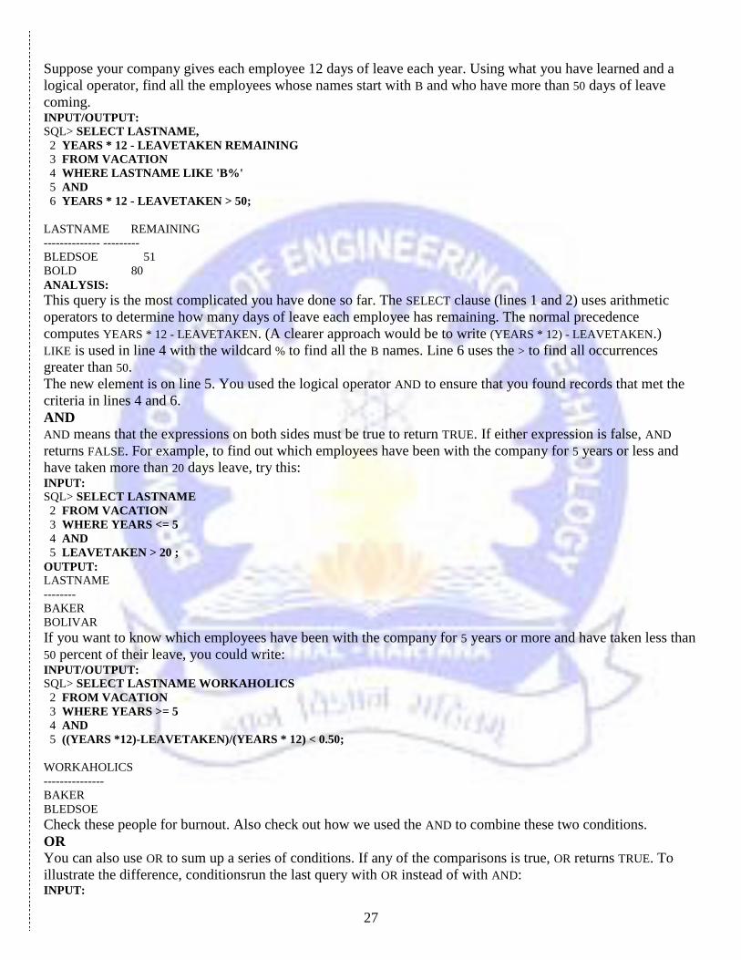
Suppose your company gives each employee 12 days of leave each year. Using what you have learned and a
logical operator, find all the employees whose names start with B and who have more than 50 days of leave
coming. INPUT/OUTPUT:
SQL> SELECT LASTNAME,
2 YEARS * 12 - LEAVETAKEN REMAINING
3 FROM VACATION
4 WHERE LASTNAME LIKE 'B%'
5 AND
6 YEARS * 12 - LEAVETAKEN > 50;
LASTNAME REMAINING
-------------- ---------
BLEDSOE 51
BOLD 80
ANALYSIS:
This query is the most complicated you have done so far. The SELECT clause (lines 1 and 2) uses arithmetic
operators to determine how many days of leave each employee has remaining. The normal precedence
computes YEARS * 12 - LEAVETAKEN. (A clearer approach would be to write (YEARS * 12) - LEAVETAKEN.)
LIKE is used in line 4 with the wildcard % to find all the B names. Line 6 uses the > to find all occurrences
greater than 50.
The new element is on line 5. You used the logical operator AND to ensure that you found records that met the
criteria in lines 4 and 6.
AND
AND means that the expressions on both sides must be true to return TRUE. If either expression is false, AND
returns FALSE. For example, to find out which employees have been with the company for 5 years or less and
have taken more than 20 days leave, try this: INPUT:
SQL> SELECT LASTNAME
2 FROM VACATION
3 WHERE YEARS <= 5
4 AND
5 LEAVETAKEN > 20 ;
OUTPUT:
LASTNAME
--------
BAKER
BOLIVAR
If you want to know which employees have been with the company for 5 years or more and have taken less than
50 percent of their leave, you could write: INPUT/OUTPUT:
SQL> SELECT LASTNAME WORKAHOLICS
2 FROM VACATION
3 WHERE YEARS >= 5
4 AND
5 ((YEARS *12)-LEAVETAKEN)/(YEARS * 12) < 0.50;
WORKAHOLICS
---------------
BAKER
BLEDSOE
Check these people for burnout. Also check out how we used the AND to combine these two conditions.
OR
You can also use OR to sum up a series of conditions. If any of the comparisons is true, OR returns TRUE. To
illustrate the difference, conditionsrun the last query with OR instead of with AND: INPUT:
28
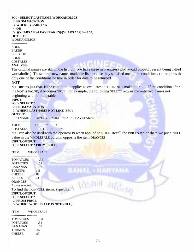
SQL> SELECT LASTNAME WORKAHOLICS
2 FROM VACATION
3 WHERE YEARS >= 5
4 OR
5 ((YEARS *12)-LEAVETAKEN)/(YEARS * 12) >= 0.50;
OUTPUT:
WORKAHOLICS
---------------
ABLE
BAKER
BLEDSOE
BOLD
COSTALES
ANALYSIS:
The original names are still in the list, but you have three new entries (who would probably resent being called
workaholics). These three new names made the list because they satisfied one of the conditions. OR requires that
only one of the conditions be true in order for data to be returned.
NOT
NOT means just that. If the condition it applies to evaluates to TRUE, NOT make it FALSE. If the condition after
the NOT is FALSE, it becomes TRUE. For example, the following SELECT returns the only two names not
beginning with B in the table: INPUT:
SQL> SELECT *
2 FROM VACATION
3 WHERE LASTNAME NOT LIKE 'B%';
OUTPUT:
LASTNAME EMPLOYEENUM YEARS LEAVETAKEN
-------------- ----------- -------- ----------
ABLE 101 2 4
COSTALES 211 10 78
NOT can also be used with the operator IS when applied to NULL. Recall the PRICES table where we put a NULL
value in the WHOLESALE column opposite the item ORANGES. INPUT/OUTPUT:
SQL> SELECT * FROM PRICE;
ITEM WHOLESALE
-------------- ---------
TOMATOES .34
POTATOES .51
BANANAS .67
TURNIPS .45
CHEESE .89
APPLES .23
ORANGES
7 rows selected.
To find the non-NULL items, type this: INPUT/OUTPUT:
SQL> SELECT *
2 FROM PRICE
3 WHERE WHOLESALE IS NOT NULL;
ITEM WHOLESALE
-------------- ---------
TOMATOES .34
POTATOES .51
BANANAS .67
TURNIPS .45
CHEESE .89

29
APPLES .23
6 rows selected.
Set Operators
UNION and UNION ALL
UNION returns the results of two queries minus the duplicate rows. The following two tables represent the
rosters of teams: INPUT:
SQL> SELECT * FROM FOOTBALL;
OUTPUT:
NAME
--------------------
ABLE
BRAVO
CHARLIE
DECON
EXITOR
FUBAR
GOOBER
7 rows selected.
INPUT:
SQL> SELECT * FROM SOFTBALL;
OUTPUT:
NAME
--------------------
ABLE
BAKER
CHARLIE
DEAN
EXITOR
FALCONER
GOOBER
7 rows selected.
How many different people play on one team or another? INPUT/OUTPUT:
SQL> SELECT NAME FROM SOFTBALL
2 UNION
3 SELECT NAME FROM FOOTBALL;
NAME
--------------------
ABLE
BAKER
BRAVO
CHARLIE
DEAN
DECON
EXITOR
FALCONER
FUBAR
GOOBER
10 rows selected.
UNION returns 10 distinct names from the two lists. How many names are on both lists (including duplicates)? INPUT/OUTPUT:
SQL> SELECT NAME FROM SOFTBALL
2 UNION ALL
3 SELECT NAME FROM FOOTBALL;
NAME
--------------------
30
ABLE
BAKER
CHARLIE
DEAN
EXITOR
FALCONER
GOOBER
ABLE
BRAVO
CHARLIE
DECON
EXITOR
FUBAR
GOOBER
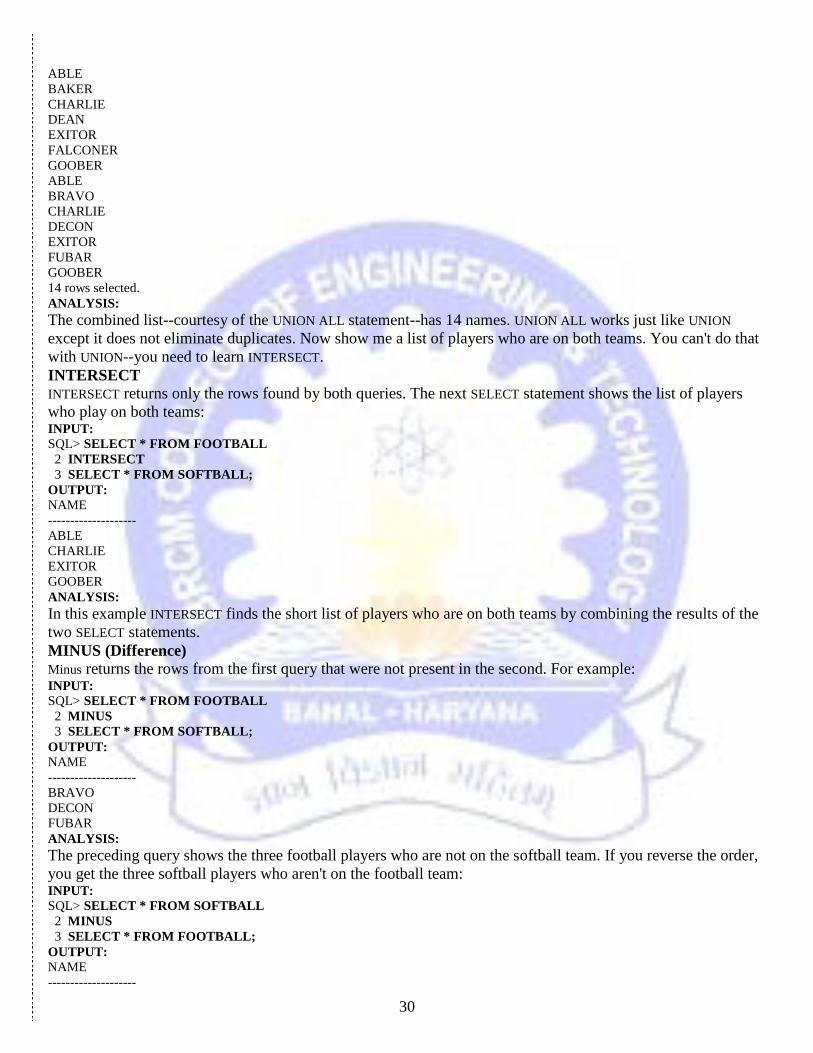
14 rows selected.
ANALYSIS:
The combined list--courtesy of the UNION ALL statement--has 14 names. UNION ALL works just like UNION
except it does not eliminate duplicates. Now show me a list of players who are on both teams. You can't do that
with UNION--you need to learn INTERSECT.
INTERSECT
INTERSECT returns only the rows found by both queries. The next SELECT statement shows the list of players
who play on both teams: INPUT:
SQL> SELECT * FROM FOOTBALL
2 INTERSECT
3 SELECT * FROM SOFTBALL;
OUTPUT:
NAME
--------------------
ABLE
CHARLIE
EXITOR
GOOBER
ANALYSIS:
In this example INTERSECT finds the short list of players who are on both teams by combining the results of the
two SELECT statements.
MINUS (Difference)
Minus returns the rows from the first query that were not present in the second. For example: INPUT:
SQL> SELECT * FROM FOOTBALL
2 MINUS
3 SELECT * FROM SOFTBALL;
OUTPUT:
NAME
--------------------
BRAVO
DECON
FUBAR
ANALYSIS:
The preceding query shows the three football players who are not on the softball team. If you reverse the order,
you get the three softball players who aren't on the football team: INPUT:
SQL> SELECT * FROM SOFTBALL
2 MINUS
3 SELECT * FROM FOOTBALL;
OUTPUT:
NAME
--------------------
31
BAKER
DEAN
FALCONER
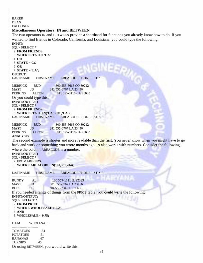
Miscellaneous Operators: IN and BETWEEN
The two operators IN and BETWEEN provide a shorthand for functions you already know how to do. If you
wanted to find friends in Colorado, California, and Louisiana, you could type the following: INPUT:
SQL> SELECT *
2 FROM FRIENDS
3 WHERE STATE= 'CA'
4 OR
5 STATE ='CO'
6 OR
7 STATE = 'LA';
OUTPUT:
LASTNAME FIRSTNAME AREACODE PHONE ST ZIP
-------------- -------------- --------- -------- -- -----
MERRICK BUD 300 555-6666 CO 80212
MAST JD 381 555-6767 LA 23456
PERKINS ALTON 911 555-3116 CA 95633
Or you could type this: INPUT/OUTPUT:
SQL> SELECT *
2 FROM FRIENDS
3 WHERE STATE IN('CA','CO','LA');
LASTNAME FIRSTNAME AREACODE PHONE ST ZIP
-------------- -------------- --------- -------- -- -----
MERRICK BUD 300 555-6666 CO 80212
MAST JD 381 555-6767 LA 23456
PERKINS ALTON 911 555-3116 CA 95633
ANALYSIS:
The second example is shorter and more readable than the first. You never know when you might have to go
back and work on something you wrote months ago. IN also works with numbers. Consider the following,
where the column AREACODE is a number: INPUT/OUTPUT:
SQL> SELECT *
2 FROM FRIENDS
3 WHERE AREACODE IN(100,381,204);
LASTNAME FIRSTNAME AREACODE PHONE ST ZIP
-------------- -------------- --------- -------- -- -----
BUNDY AL 100 555-1111 IL 22333
MAST JD 381 555-6767 LA 23456
BOSS SIR 204 555-2345 CT 95633
If you needed a range of things from the PRICE table, you could write the following: INPUT/OUTPUT:
SQL> SELECT *
2 FROM PRICE
3 WHERE WHOLESALE > 0.25
4 AND
5 WHOLESALE < 0.75;
ITEM WHOLESALE
-------------- ---------
TOMATOES .34
POTATOES .51
BANANAS .67
TURNIPS .45
Or using BETWEEN, you would write this:

32
INPUT/OUTPUT:
SQL> SELECT *
2 FROM PRICE
3 WHERE WHOLESALE BETWEEN 0.25 AND 0.75;
ITEM WHOLESALE
-------------- ---------
TOMATOES .34
POTATOES .51
BANANAS .67
TURNIPS .45
Again, the second example is a cleaner, more readable solution than the first.
PROGRAM 4 : Introduction to Different Clauses in SQL
Objectives WHERE STARTING WITH ORDER BY GROUP BY HAVING
The WHERE Clause Using just SELECT and FROM, you are limited to returning every row in a table. For
example, using these two key words on the CHECKS table, you get all seven rows: INPUT:
SQL> SELECT *
2 FROM CHECKS;
OUTPUT:
CHECK# PAYEE AMOUNT REMARKS
-------- -------------------- -------- ------------------
1 Ma Bell 150 Have sons next time
2 Reading R.R. 245.34 Train to Chicago
3 Ma Bell 200.32 Cellular Phone
4 Local Utilities 98 Gas
5 Joes Stale $ Dent 150 Groceries
16 Cash 25 Wild Night Out
17 Joans Gas 25.1 Gas
7 rows selected.
With WHERE in your vocabulary, you can be more selective. To find all the checks you wrote with a value of
more than 100 dollars, write this: INPUT:
SQL> SELECT *
2 FROM CHECKS
3 WHERE AMOUNT > 100;
The WHERE clause returns the four instances in the table that meet the required condition: OUTPUT:
CHECK# PAYEE AMOUNT REMARKS
-------- -------------------- -------- ------------------
1 Ma Bell 150 Have sons next time
2 Reading R.R. 245.34 Train to Chicago
3 Ma Bell 200.32 Cellular Phone
5 Joes Stale $ Dent 150 Groceries
WHERE can also solve other popular puzzles. Given the following table of names and locations, you can ask that
popular question, Where's Waldo? INPUT:
SQL> SELECT *
2 FROM PUZZLE;
OUTPUT:

33
NAME LOCATION
-------------- --------------
TYLER BACKYARD
MAJOR KITCHEN
SPEEDY LIVING ROOM
WALDO GARAGE
LADDIE UTILITY CLOSET
ARNOLD TV ROOM
6 rows selected.
INPUT:
SQL> SELECT LOCATION AS "WHERE'S WALDO?"
2 FROM PUZZLE
3 WHERE NAME = 'WALDO';
OUTPUT:
WHERE'S WALDO?
--------------
GARAGE
INPUT:
SQL> SELECT LOCATION "WHERE'S WALDO?"
2 FROM PUZZLE
3 WHERE NAME ='WALDO';
and get the same result as the previous query without using AS: OUTPUT:
WHERE'S WALDO?
--------------
GARAGE
After SELECT and FROM, WHERE is the third most frequently used SQL term.
The STARTING WITH Clause
STARTING WITH is an addition to the WHERE clause that works exactly like LIKE(<exp>%). Compare the results
of the following query: INPUT:
SELECT PAYEE, AMOUNT, REMARKS
FROM CHECKS
WHERE PAYEE LIKE('Ca%');
OUTPUT:
PAYEE AMOUNT REMARKS
==================== =============== ==============
Cash 25 Wild Night Out
Cash 60 Trip to Boston
Cash 34 Trip to Dayton
with the results from this query: INPUT:
SELECT PAYEE, AMOUNT, REMARKS
FROM CHECKS
WHERE PAYEE STARTING WITH('Ca');
OUTPUT:
PAYEE AMOUNT REMARKS
==================== =============== ==============
Cash 25 Wild Night Out
Cash 60 Trip to Boston
Cash 34 Trip to Dayton
The results are identical. You can even use them together, as shown here: INPUT:
SELECT PAYEE, AMOUNT, REMARKS
FROM CHECKS
WHERE PAYEE STARTING WITH('Ca')
OR
REMARKS LIKE 'G%';
OUTPUT:

34
PAYEE AMOUNT REMARKS
==================== =============== ===============
Local Utilities 98 Gas
Joes Stale $ Dent 150 Groceries
Cash 25 Wild Night Out
Joans Gas 25.1 Gas
Cash 60 Trip to Boston
Cash 34 Trip to Dayton
Joans Gas 15.75 Gas
The ORDER BY Clause INPUT:
SQL> SELECT * FROM CHECKS;
OUTPUT:
CHECK# PAYEE AMOUNT REMARKS
-------- -------------------- -------- ------------------
1 Ma Bell 150 Have sons next time
2 Reading R.R. 245.34 Train to Chicago
3 Ma Bell 200.32 Cellular Phone
4 Local Utilities 98 Gas
5 Joes Stale $ Dent 150 Groceries
16 Cash 25 Wild Night Out
17 Joans Gas 25.1 Gas
9 Abes Cleaners 24.35 X-Tra Starch
20 Abes Cleaners 10.5 All Dry Clean
8 Cash 60 Trip to Boston
21 Cash 34 Trip to Dayton
11 rows selected.
ANALYSIS:
You're going to have to trust me on this one, but the order of the output is exactly the same order as the order in
which the data was entered. After you read Day 8, "Manipulating Data," and know how to use INSERT to create
tables, you can test how data is ordered by default on your own.
The ORDER BY clause gives you a way of ordering your results. For example, to order the preceding listing by
check number, you would use the following ORDER BY clause: INPUT:
SQL> SELECT *
2 FROM CHECKS
3 ORDER BY CHECK#;
OUTPUT:
CHECK# PAYEE AMOUNT REMARKS
-------- -------------------- -------- ------------------
1 Ma Bell 150 Have sons next time
2 Reading R.R. 245.34 Train to Chicago
3 Ma Bell 200.32 Cellular Phone
4 Local Utilities 98 Gas
5 Joes Stale $ Dent 150 Groceries
8 Cash 60 Trip to Boston
9 Abes Cleaners 24.35 X-Tra Starch
16 Cash 25 Wild Night Out
17 Joans Gas 25.1 Gas
20 Abes Cleaners 10.5 All Dry Clean
21 Cash 34 Trip to Dayton
11 rows selected.
Now the data is ordered the way you want it, not the way in which it was entered. As the following example
shows, ORDER requires BY; BY is not optional. INPUT/OUTPUT:
SQL> SELECT * FROM CHECKS ORDER CHECK#;
SELECT * FROM CHECKS ORDER CHECK#
*

35
ERROR at line 1:
ORA-00924: missing BY keyword
INPUT/OUTPUT:
SQL> SELECT *
2 FROM CHECKS
3 ORDER BY PAYEE DESC;
CHECK# PAYEE AMOUNT REMARKS
-------- -------------------- -------- ------------------
2 Reading R.R. 245.34 Train to Chicago
1 Ma Bell 150 Have sons next time
3 Ma Bell 200.32 Cellular Phone
4 Local Utilities 98 Gas
5 Joes Stale $ Dent 150 Groceries
17 Joans Gas 25.1 Gas
16 Cash 25 Wild Night Out
8 Cash 60 Trip to Boston
21 Cash 34 Trip to Dayton
9 Abes Cleaners 24.35 X-Tra Starch
20 Abes Cleaners 10.5 All Dry Clean
11 rows selected.
ANALYSIS:
The DESC at the end of the ORDER BY clause orders the list in descending order instead of the default
(ascending) order. The rarely used, optional keyword ASC appears in the following statement: INPUT:
SQL> SELECT PAYEE, AMOUNT
2 FROM CHECKS
3 ORDER BY CHECK# ASC;
OUTPUT:
PAYEE AMOUNT
-------------------- ---------
Ma Bell 150
Reading R.R. 245.34
Ma Bell 200.32
Local Utilities 98
Joes Stale $ Dent 150
Cash 60
Abes Cleaners 24.35
Cash 25
Joans Gas 25.1
Abes Cleaners 10.5
Cash 34
11 rows selected.
ANALYSIS:
The ordering in this list is identical to the ordering of the list at the beginning of the section (without ASC)
because ASC is the default. This query also shows that the expression used after the ORDER BY clause does not
have to be in the SELECT statement. Although you selected only PAYEE and AMOUNT, you were still able to
order the list by CHECK#.
You can also use ORDER BY on more than one field. To order CHECKS by PAYEE and REMARKS, you would
query as follows: INPUT:
SQL> SELECT *
2 FROM CHECKS
3 ORDER BY PAYEE, REMARKS;
OUTPUT:
CHECK# PAYEE AMOUNT REMARKS
-------- -------------------- -------- ------------------

36
20 Abes Cleaners 10.5 All Dry Clean
9 Abes Cleaners 24.35 X-Tra Starch
8 Cash 60 Trip to Boston
21 Cash 34 Trip to Dayton
16 Cash 25 Wild Night Out
17 Joans Gas 25.1 Gas
5 Joes Stale $ Dent 150 Groceries
4 Local Utilities 98 Gas
3 Ma Bell 200.32 Cellular Phone
1 Ma Bell 150 Have sons next time
2 Reading R.R. 245.34 Train to Chicago
ANALYSIS:
Notice the entries for Cash in the PAYEE column. In the previous ORDER BY, the CHECK#s were in the order 16,
21, 8. Adding the field REMARKS to the ORDER BY clause puts the entries in alphabetical order according to
REMARKS. Does the order of multiple columns in the ORDER BY clause make a difference? Try the same query
again but reverse PAYEE and REMARKS: INPUT:
SQL> SELECT *
2 FROM CHECKS
3 ORDER BY REMARKS, PAYEE;
OUTPUT:
CHECK# PAYEE AMOUNT REMARKS
-------- -------------------- -------- --------------------
20 Abes Cleaners 10.5 All Dry Clean
3 Ma Bell 200.32 Cellular Phone
17 Joans Gas 25.1 Gas
4 Local Utilities 98 Gas
5 Joes Stale $ Dent 150 Groceries
1 Ma Bell 150 Have sons next time
2 Reading R.R. 245.34 Train to Chicago
8 Cash 60 Trip to Boston
21 Cash 34 Trip to Dayton
16 Cash 25 Wild Night Out
9 Abes Cleaners 24.35 X-Tra Starch
11 rows selected.
ANALYSIS:
As you probably guessed, the results are completely different. Here's how to list one column in alphabetical
order and list the second column in reverse alphabetical order: INPUT/OUTPUT:
SQL> SELECT *
2 FROM CHECKS
3 ORDER BY PAYEE ASC, REMARKS DESC;
CHECK# PAYEE AMOUNT REMARKS
-------- -------------------- -------- ------------------
9 Abes Cleaners 24.35 X-Tra Starch
20 Abes Cleaners 10.5 All Dry Clean
16 Cash 25 Wild Night Out
21 Cash 34 Trip to Dayton
8 Cash 60 Trip to Boston
17 Joans Gas 25.1 Gas
5 Joes Stale $ Dent 150 Groceries
4 Local Utilities 98 Gas
1 Ma Bell 150 Have sons next time
3 Ma Bell 200.32 Cellular Phone
2 Reading R.R. 245.34 Train to Chicago
11 rows selected.

37
ANALYSIS:
In this example PAYEE is sorted alphabetically, and REMARKS appears in descending order. Note how the
remarks in the three checks with a PAYEE of Cash are sorted. INPUT/OUTPUT:
SQL> SELECT *
2 FROM CHECKS
3 ORDER BY 1;
CHECK# PAYEE AMOUNT REMARKS
-------- -------------------- -------- ------------------
1 Ma Bell 150 Have sons next time
2 Reading R.R. 245.34 Train to Chicago
3 Ma Bell 200.32 Cellular Phone
4 Local Utilities 98 Gas
5 Joes Stale $ Dent 150 Groceries
8 Cash 60 Trip to Boston
9 Abes Cleaners 24.35 X-Tra Starch
16 Cash 25 Wild Night Out
17 Joans Gas 25.1 Gas
20 Abes Cleaners 10.5 All Dry Clean
21 Cash 34 Trip to Dayton
11 rows selected.
ANALYSIS:
This result is identical to the result produced by the SELECT statement that you used earlier today: SELECT * FROM CHECKS ORDER BY CHECK#;
The GROUP BY Clause INPUT:
SELECT *
FROM CHECKS;
Here's the modified table: OUTPUT:
CHECKNUM PAYEE AMOUNT REMARKS
======== =========== =============== ======================
1 Ma Bell 150 Have sons next time
2 Reading R.R. 245.34 Train to Chicago
3 Ma Bell 200.33 Cellular Phone
4 Local Utilities 98 Gas
5 Joes Stale $ Dent 150 Groceries
16 Cash 25 Wild Night Out
17 Joans Gas 25.1 Gas
9 Abes Cleaners 24.35 X-Tra Starch
20 Abes Cleaners 10.5 All Dry Clean
8 Cash 60 Trip to Boston
21 Cash 34 Trip to Dayton
30 Local Utilities 87.5 Water
31 Local Utilities 34 Sewer
25 Joans Gas 15.75 Gas
Then you would type: INPUT/OUTPUT:
SELECT SUM(AMOUNT)
FROM CHECKS;
SUM
===============
1159.87
ANALYSIS:

38
This statement returns the sum of the column AMOUNT. What if you wanted to find out how much you have
spent on each PAYEE? SQL helps you with the GROUP BY clause. To find out whom you have paid and how
much, you would query like this: INPUT/OUTPUT:
SELECT PAYEE, SUM(AMOUNT)
FROM CHECKS
GROUP BY PAYEE;
PAYEE SUM
==================== ===============
Abes Cleaners 34.849998
Cash 119
Joans Gas 40.849998
Joes Stale $ Dent 150
Local Utilities 219.5
Ma Bell 350.33002
Reading R.R. 245.34
ANALYSIS:
The SELECT clause has a normal column selection, PAYEE, followed by the aggregate function SUM(AMOUNT).
If you had tried this query with only the FROM CHECKS that follows, here's what you would see: INPUT/OUTPUT:
SELECT PAYEE, SUM(AMOUNT)
FROM CHECKS;
Dynamic SQL Error
-SQL error code = -104
-invalid column reference
ANALYSIS:
SQL is complaining about the combination of the normal column and the aggregate function. This condition
requires the GROUP BY clause. GROUP BY runs the aggregate function described in the SELECT statement for
each grouping of the column that follows the GROUP BY clause. The table CHECKS returned 14 rows when
queried with SELECT * FROM CHECKS. The query on the same table, SELECT PAYEE, SUM(AMOUNT) FROM
CHECKS GROUP BY PAYEE, took the 14 rows in the table and made seven groupings, INPUT/OUTPUT:
SELECT PAYEE, SUM(AMOUNT), COUNT(PAYEE)
FROM CHECKS
GROUP BY PAYEE;
PAYEE SUM COUNT
==================== =============== ===========
Abes Cleaners 34.849998 2
Cash 119 3
Joans Gas 40.849998 2
Joes Stale $ Dent 150 1
Local Utilities 219.5 3
Ma Bell 350.33002 2
Reading R.R. 245.34 1
ANALYSIS:
This SQL is becoming increasingly useful! In the preceding example, you were able to perform group functions
on unique groups using the GROUP BY clause. Also notice that the results were ordered by payee. GROUP BY
also acts like the ORDER BY clause. What would happen if you tried to group by more than one column? Try
this: INPUT/OUTPUT:
SELECT PAYEE, SUM(AMOUNT), COUNT(PAYEE)
FROM CHECKS
GROUP BY PAYEE, REMARKS;
39
PAYEE SUM COUNT
==================== =============== ===========
Abes Cleaners 10.5 1
Abes Cleaners 24.35 1
Cash 60 1
Cash 34 1
Cash 25 1
Joans Gas 40.849998 2
Joes Stale $ Dent 150 1
Local Utilities 98 1
Local Utilities 34 1
Local Utilities 87.5 1
Ma Bell 200.33 1
Ma Bell 150 1
Reading R.R. 245.34 1
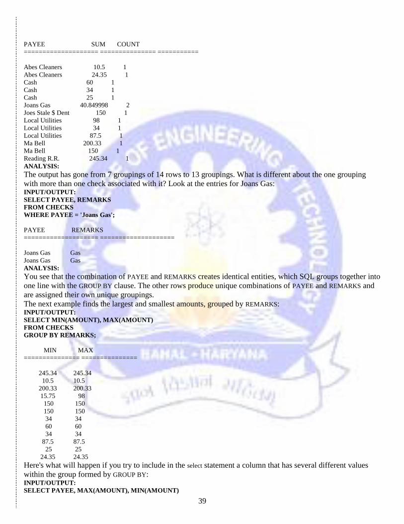
ANALYSIS:
The output has gone from 7 groupings of 14 rows to 13 groupings. What is different about the one grouping
with more than one check associated with it? Look at the entries for Joans Gas: INPUT/OUTPUT:
SELECT PAYEE, REMARKS
FROM CHECKS
WHERE PAYEE = 'Joans Gas';
PAYEE REMARKS
==================== ====================
Joans Gas Gas
Joans Gas Gas
ANALYSIS:
You see that the combination of PAYEE and REMARKS creates identical entities, which SQL groups together into
one line with the GROUP BY clause. The other rows produce unique combinations of PAYEE and REMARKS and
are assigned their own unique groupings.
The next example finds the largest and smallest amounts, grouped by REMARKS: INPUT/OUTPUT:
SELECT MIN(AMOUNT), MAX(AMOUNT)
FROM CHECKS
GROUP BY REMARKS;
MIN MAX
=============== ===============
245.34 245.34
10.5 10.5
200.33 200.33
15.75 98
150 150
150 150
34 34
60 60
34 34
87.5 87.5
25 25
24.35 24.35
Here's what will happen if you try to include in the select statement a column that has several different values
within the group formed by GROUP BY: INPUT/OUTPUT:
SELECT PAYEE, MAX(AMOUNT), MIN(AMOUNT)
40
FROM CHECKS
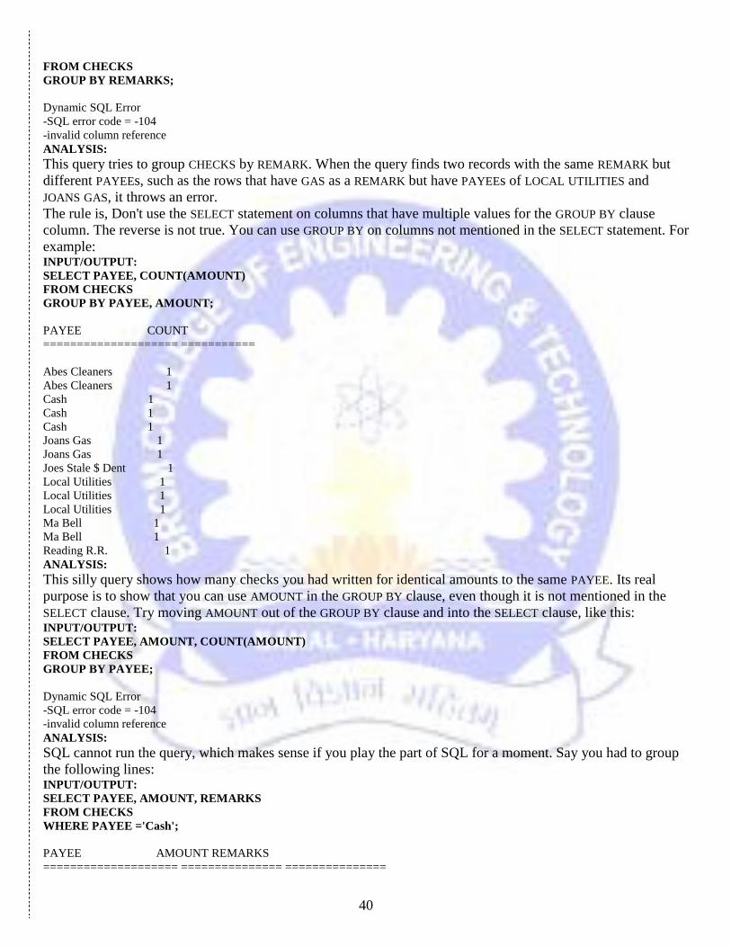
GROUP BY REMARKS;
Dynamic SQL Error
-SQL error code = -104
-invalid column reference
ANALYSIS:
This query tries to group CHECKS by REMARK. When the query finds two records with the same REMARK but
different PAYEEs, such as the rows that have GAS as a REMARK but have PAYEEs of LOCAL UTILITIES and
JOANS GAS, it throws an error.
The rule is, Don't use the SELECT statement on columns that have multiple values for the GROUP BY clause
column. The reverse is not true. You can use GROUP BY on columns not mentioned in the SELECT statement. For
example: INPUT/OUTPUT:
SELECT PAYEE, COUNT(AMOUNT)
FROM CHECKS
GROUP BY PAYEE, AMOUNT;
PAYEE COUNT
==================== ===========
Abes Cleaners 1
Abes Cleaners 1
Cash 1
Cash 1
Cash 1
Joans Gas 1
Joans Gas 1
Joes Stale $ Dent 1
Local Utilities 1
Local Utilities 1
Local Utilities 1
Ma Bell 1
Ma Bell 1
Reading R.R. 1
ANALYSIS:
This silly query shows how many checks you had written for identical amounts to the same PAYEE. Its real
purpose is to show that you can use AMOUNT in the GROUP BY clause, even though it is not mentioned in the
SELECT clause. Try moving AMOUNT out of the GROUP BY clause and into the SELECT clause, like this: INPUT/OUTPUT:
SELECT PAYEE, AMOUNT, COUNT(AMOUNT)
FROM CHECKS
GROUP BY PAYEE;
Dynamic SQL Error
-SQL error code = -104
-invalid column reference
ANALYSIS:
SQL cannot run the query, which makes sense if you play the part of SQL for a moment. Say you had to group
the following lines: INPUT/OUTPUT:
SELECT PAYEE, AMOUNT, REMARKS
FROM CHECKS
WHERE PAYEE ='Cash';
PAYEE AMOUNT REMARKS
==================== =============== ===============
41
Cash 25 Wild Night Out
Cash 60 Trip to Boston
Cash 34 Trip to Dayton
If the user asked you to output all three columns and group by PAYEE only, where would you put the unique
remarks? Remember you have only one row per group when you use GROUP BY. SQL can't do two things at
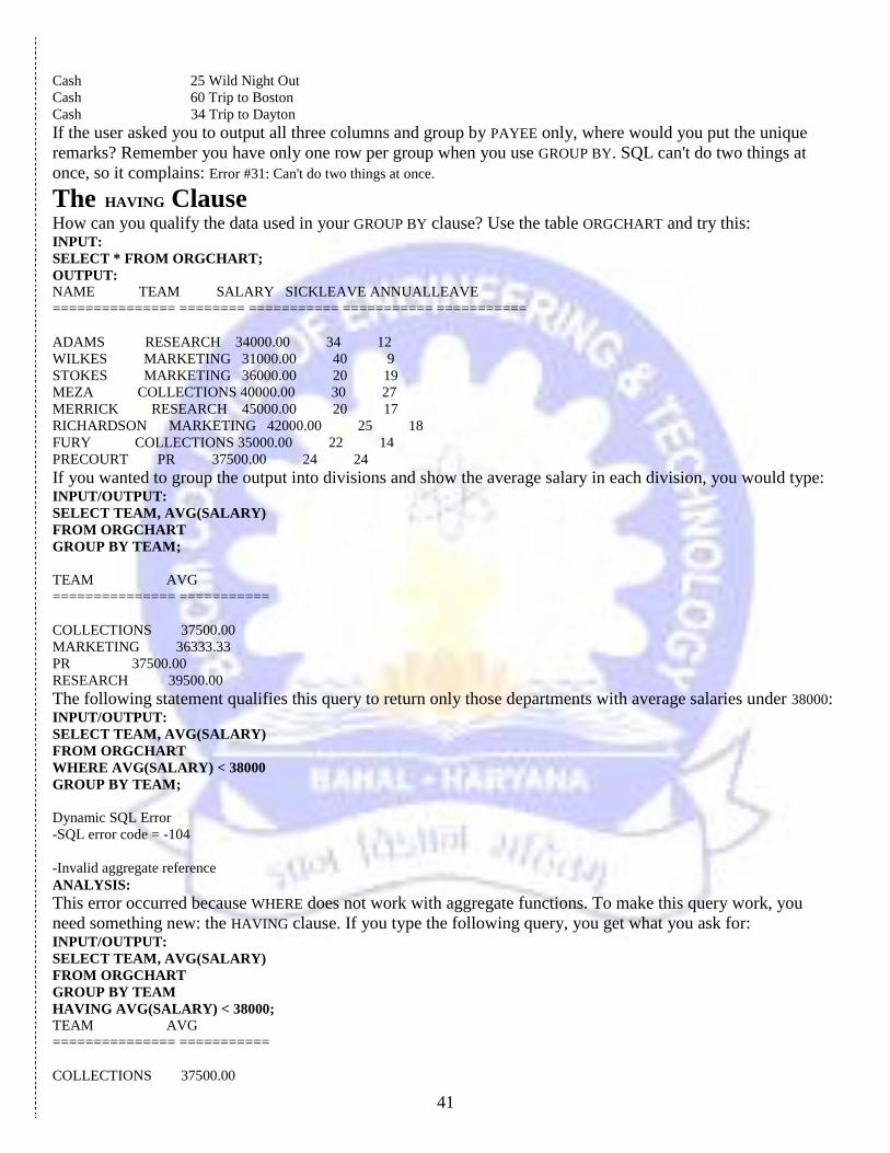
once, so it complains: Error #31: Can't do two things at once.
The HAVING Clause How can you qualify the data used in your GROUP BY clause? Use the table ORGCHART and try this: INPUT:
SELECT * FROM ORGCHART;
OUTPUT:
NAME TEAM SALARY SICKLEAVE ANNUALLEAVE
=============== ======== =========== =========== ===========
ADAMS RESEARCH 34000.00 34 12
WILKES MARKETING 31000.00 40 9
STOKES MARKETING 36000.00 20 19
MEZA COLLECTIONS 40000.00 30 27
MERRICK RESEARCH 45000.00 20 17
RICHARDSON MARKETING 42000.00 25 18
FURY COLLECTIONS 35000.00 22 14
PRECOURT PR 37500.00 24 24
If you wanted to group the output into divisions and show the average salary in each division, you would type: INPUT/OUTPUT:
SELECT TEAM, AVG(SALARY)
FROM ORGCHART
GROUP BY TEAM;
TEAM AVG
=============== ===========
COLLECTIONS 37500.00
MARKETING 36333.33
PR 37500.00
RESEARCH 39500.00
The following statement qualifies this query to return only those departments with average salaries under 38000: INPUT/OUTPUT:
SELECT TEAM, AVG(SALARY)
FROM ORGCHART
WHERE AVG(SALARY) < 38000
GROUP BY TEAM;
Dynamic SQL Error
-SQL error code = -104
-Invalid aggregate reference
ANALYSIS:
This error occurred because WHERE does not work with aggregate functions. To make this query work, you
need something new: the HAVING clause. If you type the following query, you get what you ask for: INPUT/OUTPUT:
SELECT TEAM, AVG(SALARY)
FROM ORGCHART
GROUP BY TEAM
HAVING AVG(SALARY) < 38000; TEAM AVG
=============== ===========
COLLECTIONS 37500.00
42
MARKETING 36333.33
PR 37500.00
ANALYSIS:
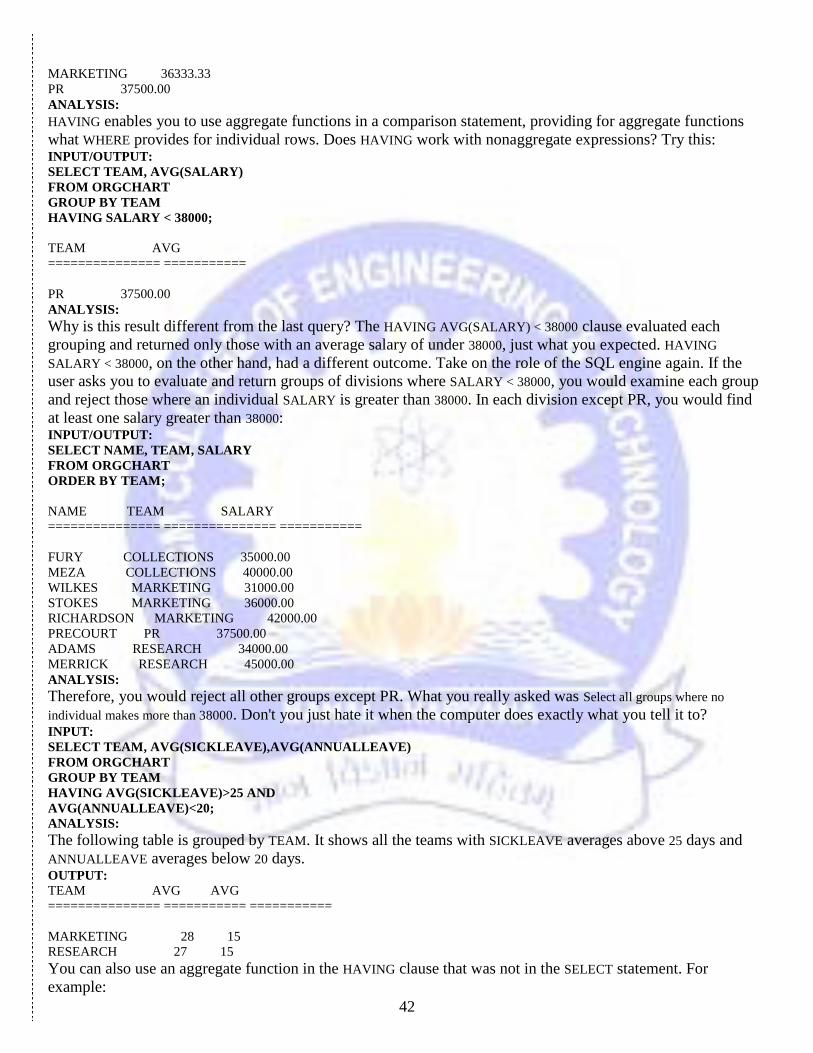
HAVING enables you to use aggregate functions in a comparison statement, providing for aggregate functions
what WHERE provides for individual rows. Does HAVING work with nonaggregate expressions? Try this: INPUT/OUTPUT:
SELECT TEAM, AVG(SALARY)
FROM ORGCHART
GROUP BY TEAM
HAVING SALARY < 38000;
TEAM AVG
=============== ===========
PR 37500.00
ANALYSIS:
Why is this result different from the last query? The HAVING AVG(SALARY) < 38000 clause evaluated each
grouping and returned only those with an average salary of under 38000, just what you expected. HAVING
SALARY < 38000, on the other hand, had a different outcome. Take on the role of the SQL engine again. If the
user asks you to evaluate and return groups of divisions where SALARY < 38000, you would examine each group
and reject those where an individual SALARY is greater than 38000. In each division except PR, you would find
at least one salary greater than 38000: INPUT/OUTPUT:
SELECT NAME, TEAM, SALARY
FROM ORGCHART
ORDER BY TEAM;
NAME TEAM SALARY
=============== =============== ===========
FURY COLLECTIONS 35000.00
MEZA COLLECTIONS 40000.00
WILKES MARKETING 31000.00
STOKES MARKETING 36000.00
RICHARDSON MARKETING 42000.00
PRECOURT PR 37500.00
ADAMS RESEARCH 34000.00
MERRICK RESEARCH 45000.00
ANALYSIS:
Therefore, you would reject all other groups except PR. What you really asked was Select all groups where no
individual makes more than 38000. Don't you just hate it when the computer does exactly what you tell it to? INPUT:
SELECT TEAM, AVG(SICKLEAVE),AVG(ANNUALLEAVE)
FROM ORGCHART
GROUP BY TEAM
HAVING AVG(SICKLEAVE)>25 AND
AVG(ANNUALLEAVE)<20;
ANALYSIS:
The following table is grouped by TEAM. It shows all the teams with SICKLEAVE averages above 25 days and
ANNUALLEAVE averages below 20 days. OUTPUT:
TEAM AVG AVG
=============== =========== ===========
MARKETING 28 15
RESEARCH 27 15
You can also use an aggregate function in the HAVING clause that was not in the SELECT statement. For
example:
43
INPUT/OUTPUT:
SELECT TEAM, AVG(SICKLEAVE),AVG(ANNUALLEAVE)
FROM ORGCHART
GROUP BY TEAM
HAVING COUNT(TEAM) > 1;
TEAM AVG AVG
=============== =========== ===========
COLLECTIONS 26 21
MARKETING 28 15
RESEARCH 27 15
ANALYSIS:
This query returns the number of TEAMs with more than one member. COUNT(TEAM) is not used in the SELECT
statement but still functions as expected in the HAVING clause.
The other logical operators all work well within the HAVING clause. Consider this: INPUT/OUTPUT:
SELECT TEAM,MIN(SALARY),MAX(SALARY)
FROM ORGCHART
GROUP BY TEAM
HAVING AVG(SALARY) > 37000
OR
MIN(SALARY) > 32000;
TEAM MIN MAX
=============== =========== ===========
COLLECTIONS 35000.00 40000.00
PR 37500.00 37500.00
RESEARCH 34000.00 45000.00
The operator IN also works in a HAVING clause, as demonstrated here: INPUT/OUTPUT:
SELECT TEAM,AVG(SALARY)
FROM ORGCHART
GROUP BY TEAM
HAVING TEAM IN ('PR','RESEARCH');
TEAM AVG
=============== ===========
PR 37500.00
RESEARCH 39500.00
Find all the checks written for Cash and Gas in the CHECKS table and order them by REMARKS. INPUT:
SELECT PAYEE, REMARKS
FROM CHECKS
WHERE PAYEE = 'Cash'
OR REMARKS LIKE'Ga%'
ORDER BY REMARKS;
OUTPUT:
PAYEE REMARKS
==================== ====================
Joans Gas Gas
Joans Gas Gas
Local Utilities Gas
Cash Trip to Boston
Cash Trip to Dayton
Cash Wild Night Out

44
ANALYSIS:
Note the use of LIKE to find the REMARKS that started with Ga. With the use of OR, data was returned if the
WHERE clause met either one of the two conditions.
What if you asked for the same information and group it by PAYEE? The query would look something like this: INPUT:
SELECT PAYEE, REMARKS
FROM CHECKS
WHERE PAYEE = 'Cash'
OR REMARKS LIKE'Ga%'
GROUP BY PAYEE
ORDER BY REMARKS;
ANALYSIS:
This query would not work because the SQL engine would not know what to do with the remarks. Remember
that whatever columns you put in the SELECT clause must also be in the GROUP BY clause--unless you don't
specify any columns in the SELECT clause.
Using the table ORGCHART, find the salary of everyone with less than 25 days of sick leave. Order the results by
NAME. INPUT:
SELECT NAME, SALARY
FROM ORGCHART
WHERE SICKLEAVE < 25
ORDER BY NAME;
OUTPUT:
NAME SALARY
=============== ===========
FURY 35000.00
MERRICK 45000.00
PRECOURT 37500.00
STOKES 36000.00
ANALYSIS:
This query is straightforward and enables you to use your new-found skills with WHERE and ORDER BY.
Again, using ORGCHART, display TEAM, AVG(SALARY), AVG(SICKLEAVE), and AVG(ANNUALLEAVE) on each
team: INPUT:
SELECT TEAM,
AVG(SALARY),
AVG(SICKLEAVE),
AVG(ANNUALLEAVE)
FROM ORGCHART
GROUP BY TEAM;
OUTPUT:
TEAM AVG AVG AVG
=============== =========== =========== ===========
COLLECTIONS 37500.00 26 21
MARKETING 36333.33 28 15
PR 37500.00 24 24
RESEARCH 39500.00 26 15
An interesting variation on this query follows. See if you can figure out what happened: INPUT/OUTPUT:
SELECT TEAM,
AVG(SALARY),
AVG(SICKLEAVE),
AVG(ANNUALLEAVE)
FROM ORGCHART
GROUP BY TEAM
ORDER BY NAME;
TEAM AVG AVG AVG

45
=============== =========== =========== ===========
RESEARCH 39500.00 27 15
COLLECTIONS 37500.00 26 21
PR 37500.00 24 24
MARKETING 36333.33 28 15
A simpler query using ORDER BY might offer a clue: INPUT/OUTPUT:
SELECT NAME, TEAM
FROM ORGCHART
ORDER BY NAME, TEAM;
NAME TEAM
=============== ===========
ADAMS RESEARCH
FURY COLLECTIONS
MERRICK RESEARCH
MEZA COLLECTIONS
PRECOURT PR
RICHARDSON MARKETING
STOKES MARKETING
WILKES MARKETING
ANALYSIS:
When the SQL engine got around to ordering the results of the query, it used the NAME column (remember, it is
perfectly legal to use a column not specified in the SELECT statement), ignored duplicate TEAM entries, and
came up with the order RESEARCH, COLLECTIONS, PR, and MARKETING. Including TEAM in the ORDER BY
clause is unnecessary, because you have unique values in the NAME column. You can get the same result by
typing this statement: INPUT/OUTPUT:
SELECT NAME, TEAM
FROM ORGCHART
ORDER BY NAME;
NAME TEAM
=============== ============
ADAMS RESEARCH
FURY COLLECTIONS
MERRICK RESEARCH
MEZA COLLECTIONS
PRECOURT PR
RICHARDSON MARKETING
STOKES MARKETING
WILKES MARKETING
While you are looking at variations, don't forget you can also reverse the order: INPUT/OUTPUT:
SELECT NAME, TEAM
FROM ORGCHART
ORDER BY NAME DESC;
NAME TEAM
=============== ============
WILKES MARKETING
STOKES MARKETING
RICHARDSON MARKETING
PRECOURT PR
MEZA COLLECTIONS
MERRICK RESEARCH
FURY COLLECTIONS
ADAMS RESEARCH
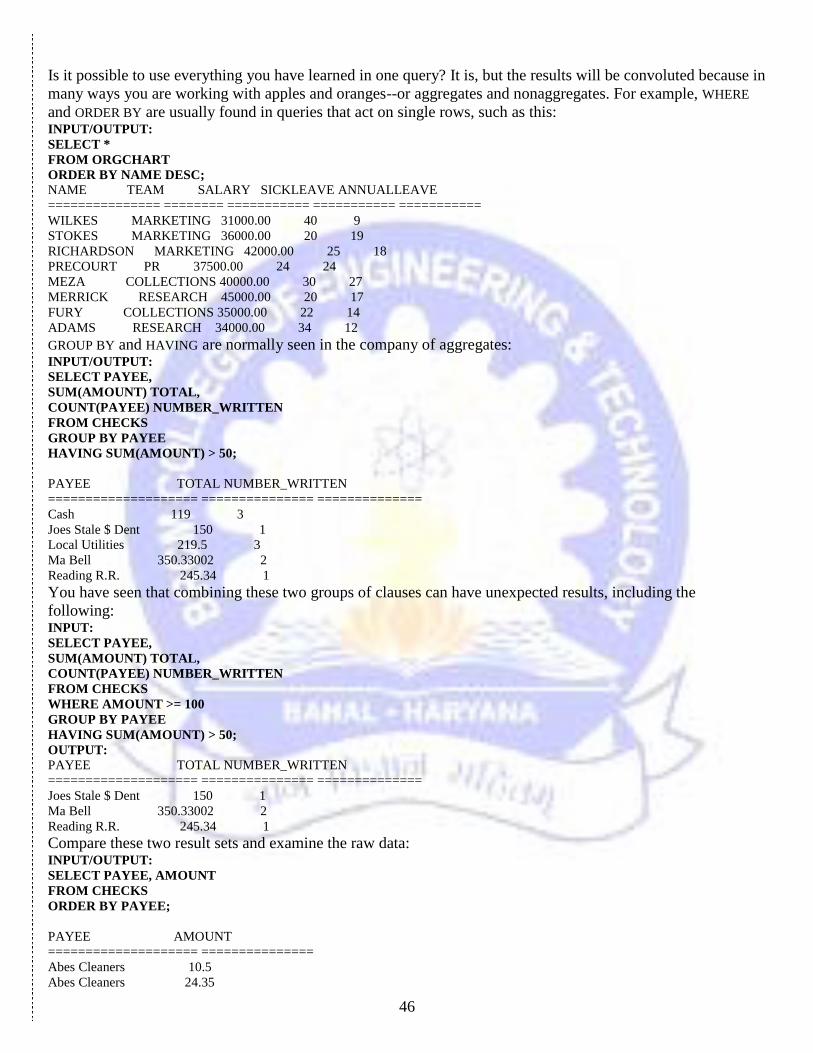
46
Is it possible to use everything you have learned in one query? It is, but the results will be convoluted because in
many ways you are working with apples and oranges--or aggregates and nonaggregates. For example, WHERE
and ORDER BY are usually found in queries that act on single rows, such as this: INPUT/OUTPUT:
SELECT *
FROM ORGCHART
ORDER BY NAME DESC; NAME TEAM SALARY SICKLEAVE ANNUALLEAVE
=============== ======== =========== =========== ===========
WILKES MARKETING 31000.00 40 9
STOKES MARKETING 36000.00 20 19
RICHARDSON MARKETING 42000.00 25 18
PRECOURT PR 37500.00 24 24
MEZA COLLECTIONS 40000.00 30 27
MERRICK RESEARCH 45000.00 20 17
FURY COLLECTIONS 35000.00 22 14
ADAMS RESEARCH 34000.00 34 12
GROUP BY and HAVING are normally seen in the company of aggregates: INPUT/OUTPUT:
SELECT PAYEE,
SUM(AMOUNT) TOTAL,
COUNT(PAYEE) NUMBER_WRITTEN
FROM CHECKS
GROUP BY PAYEE
HAVING SUM(AMOUNT) > 50;
PAYEE TOTAL NUMBER_WRITTEN
==================== =============== ==============
Cash 119 3
Joes Stale $ Dent 150 1
Local Utilities 219.5 3
Ma Bell 350.33002 2
Reading R.R. 245.34 1
You have seen that combining these two groups of clauses can have unexpected results, including the
following: INPUT:
SELECT PAYEE,
SUM(AMOUNT) TOTAL,
COUNT(PAYEE) NUMBER_WRITTEN
FROM CHECKS
WHERE AMOUNT >= 100
GROUP BY PAYEE
HAVING SUM(AMOUNT) > 50;
OUTPUT:
PAYEE TOTAL NUMBER_WRITTEN
==================== =============== ==============
Joes Stale $ Dent 150 1
Ma Bell 350.33002 2
Reading R.R. 245.34 1
Compare these two result sets and examine the raw data: INPUT/OUTPUT:
SELECT PAYEE, AMOUNT
FROM CHECKS
ORDER BY PAYEE;
PAYEE AMOUNT
==================== ===============
Abes Cleaners 10.5
Abes Cleaners 24.35
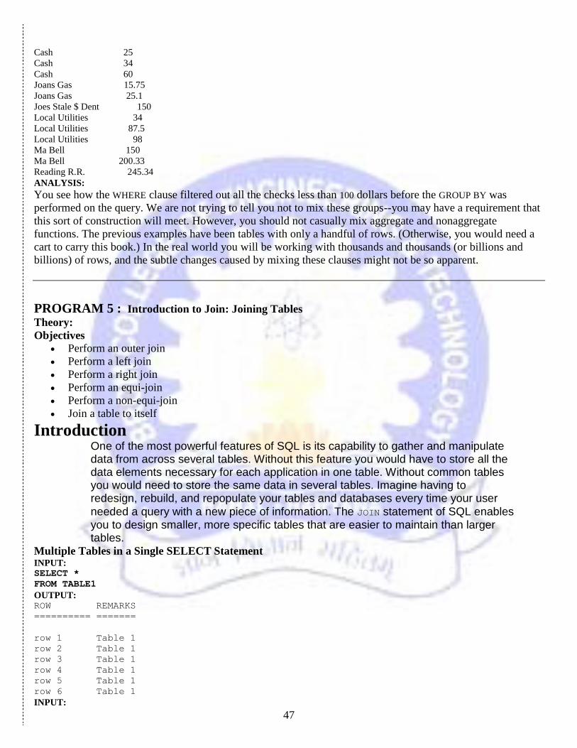
47
Cash 25
Cash 34
Cash 60
Joans Gas 15.75
Joans Gas 25.1
Joes Stale $ Dent 150
Local Utilities 34
Local Utilities 87.5
Local Utilities 98
Ma Bell 150
Ma Bell 200.33
Reading R.R. 245.34
ANALYSIS:
You see how the WHERE clause filtered out all the checks less than 100 dollars before the GROUP BY was
performed on the query. We are not trying to tell you not to mix these groups--you may have a requirement that
this sort of construction will meet. However, you should not casually mix aggregate and nonaggregate
functions. The previous examples have been tables with only a handful of rows. (Otherwise, you would need a
cart to carry this book.) In the real world you will be working with thousands and thousands (or billions and
billions) of rows, and the subtle changes caused by mixing these clauses might not be so apparent.
PROGRAM 5 : Introduction to Join: Joining Tables
Theory:
Objectives
Perform an outer join
Perform a left join
Perform a right join
Perform an equi-join
Perform a non-equi-join
Join a table to itself
Introduction One of the most powerful features of SQL is its capability to gather and manipulate data from across several tables. Without this feature you would have to store all the data elements necessary for each application in one table. Without common tables you would need to store the same data in several tables. Imagine having to redesign, rebuild, and repopulate your tables and databases every time your user
needed a query with a new piece of information. The JOIN statement of SQL enables you to design smaller, more specific tables that are easier to maintain than larger tables.
Multiple Tables in a Single SELECT Statement INPUT: SELECT *
FROM TABLE1
OUTPUT: ROW REMARKS
========== =======
row 1 Table 1
row 2 Table 1
row 3 Table 1
row 4 Table 1
row 5 Table 1
row 6 Table 1
INPUT:
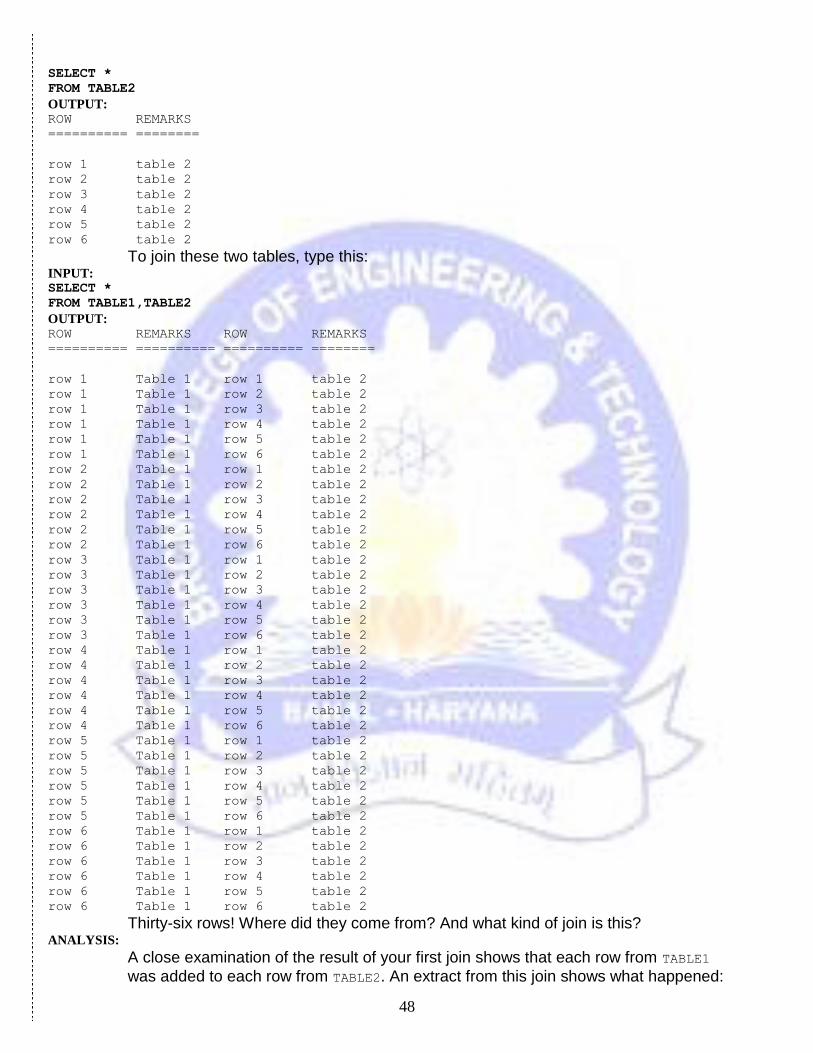
48
SELECT *
FROM TABLE2
OUTPUT: ROW REMARKS
========== ========
row 1 table 2
row 2 table 2
row 3 table 2
row 4 table 2
row 5 table 2
row 6 table 2
To join these two tables, type this: INPUT: SELECT *
FROM TABLE1,TABLE2
OUTPUT: ROW REMARKS ROW REMARKS
========== ========== ========== ========
row 1 Table 1 row 1 table 2
row 1 Table 1 row 2 table 2
row 1 Table 1 row 3 table 2
row 1 Table 1 row 4 table 2
row 1 Table 1 row 5 table 2
row 1 Table 1 row 6 table 2
row 2 Table 1 row 1 table 2
row 2 Table 1 row 2 table 2
row 2 Table 1 row 3 table 2
row 2 Table 1 row 4 table 2
row 2 Table 1 row 5 table 2
row 2 Table 1 row 6 table 2
row 3 Table 1 row 1 table 2
row 3 Table 1 row 2 table 2
row 3 Table 1 row 3 table 2
row 3 Table 1 row 4 table 2
row 3 Table 1 row 5 table 2
row 3 Table 1 row 6 table 2
row 4 Table 1 row 1 table 2
row 4 Table 1 row 2 table 2
row 4 Table 1 row 3 table 2
row 4 Table 1 row 4 table 2
row 4 Table 1 row 5 table 2
row 4 Table 1 row 6 table 2
row 5 Table 1 row 1 table 2
row 5 Table 1 row 2 table 2
row 5 Table 1 row 3 table 2
row 5 Table 1 row 4 table 2
row 5 Table 1 row 5 table 2
row 5 Table 1 row 6 table 2
row 6 Table 1 row 1 table 2
row 6 Table 1 row 2 table 2
row 6 Table 1 row 3 table 2
row 6 Table 1 row 4 table 2
row 6 Table 1 row 5 table 2
row 6 Table 1 row 6 table 2
Thirty-six rows! Where did they come from? And what kind of join is this? ANALYSIS:
A close examination of the result of your first join shows that each row from TABLE1
was added to each row from TABLE2. An extract from this join shows what happened:
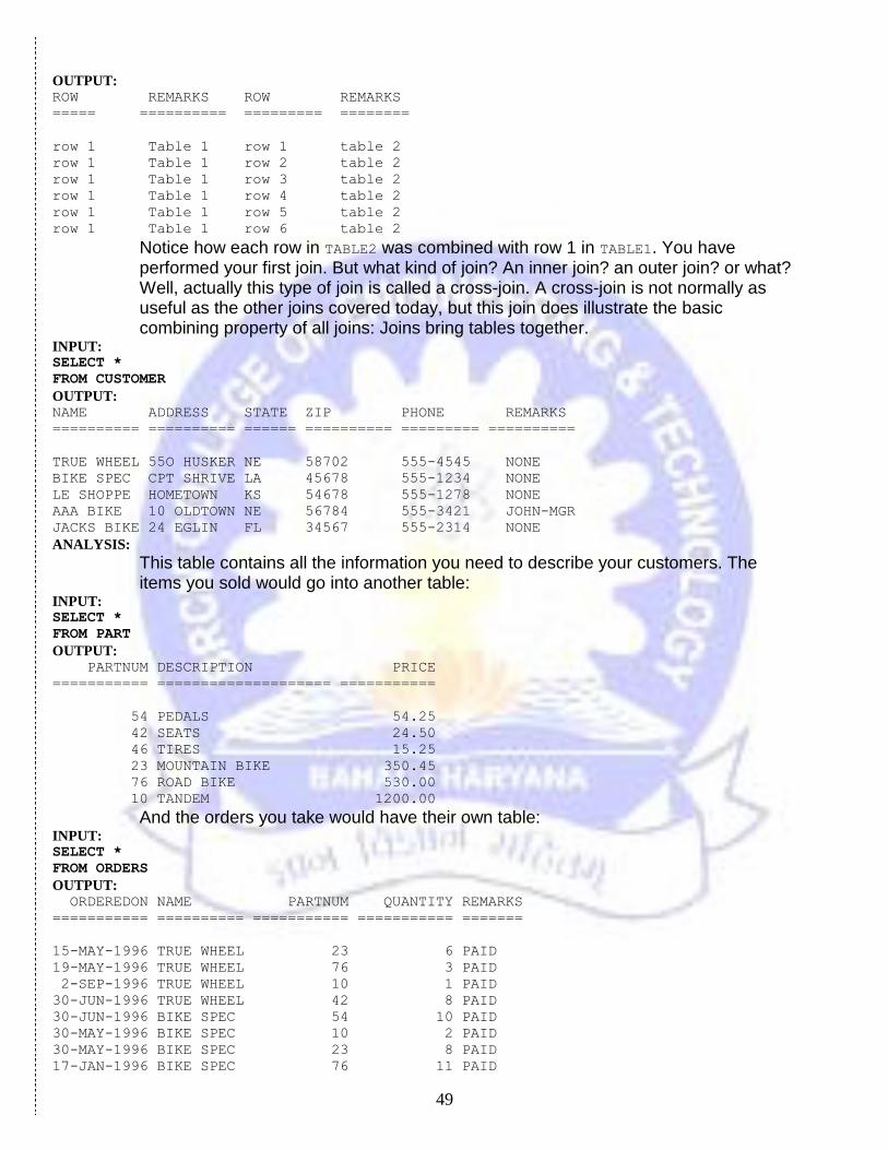
49
OUTPUT: ROW REMARKS ROW REMARKS
===== ========== ========= ========
row 1 Table 1 row 1 table 2
row 1 Table 1 row 2 table 2
row 1 Table 1 row 3 table 2
row 1 Table 1 row 4 table 2
row 1 Table 1 row 5 table 2
row 1 Table 1 row 6 table 2
Notice how each row in TABLE2 was combined with row 1 in TABLE1. You have performed your first join. But what kind of join? An inner join? an outer join? or what? Well, actually this type of join is called a cross-join. A cross-join is not normally as useful as the other joins covered today, but this join does illustrate the basic combining property of all joins: Joins bring tables together.
INPUT: SELECT *
FROM CUSTOMER
OUTPUT: NAME ADDRESS STATE ZIP PHONE REMARKS
========== ========== ====== ========== ========= ==========
TRUE WHEEL 55O HUSKER NE 58702 555-4545 NONE
BIKE SPEC CPT SHRIVE LA 45678 555-1234 NONE
LE SHOPPE HOMETOWN KS 54678 555-1278 NONE
AAA BIKE 10 OLDTOWN NE 56784 555-3421 JOHN-MGR
JACKS BIKE 24 EGLIN FL 34567 555-2314 NONE
ANALYSIS:
This table contains all the information you need to describe your customers. The items you sold would go into another table:
INPUT: SELECT *
FROM PART
OUTPUT: PARTNUM DESCRIPTION PRICE
=========== ==================== ===========
54 PEDALS 54.25
42 SEATS 24.50
46 TIRES 15.25
23 MOUNTAIN BIKE 350.45
76 ROAD BIKE 530.00
10 TANDEM 1200.00
And the orders you take would have their own table: INPUT: SELECT *
FROM ORDERS
OUTPUT: ORDEREDON NAME PARTNUM QUANTITY REMARKS
=========== ========== =========== =========== =======
15-MAY-1996 TRUE WHEEL 23 6 PAID
19-MAY-1996 TRUE WHEEL 76 3 PAID
2-SEP-1996 TRUE WHEEL 10 1 PAID
30-JUN-1996 TRUE WHEEL 42 8 PAID
30-JUN-1996 BIKE SPEC 54 10 PAID
30-MAY-1996 BIKE SPEC 10 2 PAID
30-MAY-1996 BIKE SPEC 23 8 PAID
17-JAN-1996 BIKE SPEC 76 11 PAID
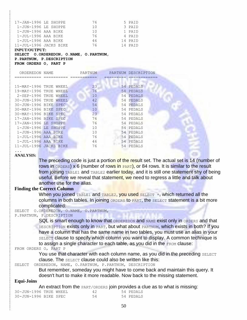
50
17-JAN-1996 LE SHOPPE 76 5 PAID
1-JUN-1996 LE SHOPPE 10 3 PAID
1-JUN-1996 AAA BIKE 10 1 PAID
1-JUL-1996 AAA BIKE 76 4 PAID
1-JUL-1996 AAA BIKE 46 14 PAID
11-JUL-1996 JACKS BIKE 76 14 PAID
INPUT/OUTPUT: SELECT O.ORDEREDON, O.NAME, O.PARTNUM,
P.PARTNUM, P.DESCRIPTION
FROM ORDERS O, PART P
ORDEREDON NAME PARTNUM PARTNUM DESCRIPTION
=========== ========== =========== ========= ============
15-MAY-1996 TRUE WHEEL 23 54 PEDALS
19-MAY-1996 TRUE WHEEL 76 54 PEDALS
2-SEP-1996 TRUE WHEEL 10 54 PEDALS
30-JUN-1996 TRUE WHEEL 42 54 PEDALS
30-JUN-1996 BIKE SPEC 54 54 PEDALS
30-MAY-1996 BIKE SPEC 10 54 PEDALS
30-MAY-1996 BIKE SPEC 23 54 PEDALS
17-JAN-1996 BIKE SPEC 76 54 PEDALS
17-JAN-1996 LE SHOPPE 76 54 PEDALS
1-JUN-1996 LE SHOPPE 10 54 PEDALS
1-JUN-1996 AAA BIKE 10 54 PEDALS
1-JUL-1996 AAA BIKE 76 54 PEDALS
1-JUL-1996 AAA BIKE 46 54 PEDALS
11-JUL-1996 JACKS BIKE 76 54 PEDALS
...
ANALYSIS:
The preceding code is just a portion of the result set. The actual set is 14 (number of
rows in ORDERS) x 6 (number of rows in PART), or 84 rows. It is similar to the result
from joining TABLE1 and TABLE2 earlier today, and it is still one statement shy of being useful. Before we reveal that statement, we need to regress a little and talk about another use for the alias.
Finding the Correct Column
When you joined TABLE1 and TABLE2, you used SELECT *, which returned all the
columns in both tables. In joining ORDERS to PART, the SELECT statement is a bit more complicated:
SELECT O.ORDEREDON, O.NAME, O.PARTNUM,
P.PARTNUM, P.DESCRIPTION
SQL is smart enough to know that ORDEREDON and NAME exist only in ORDERS and that
DESCRIPTION exists only in PART, but what about PARTNUM, which exists in both? If you have a column that has the same name in two tables, you must use an alias in your
SELECT clause to specify which column you want to display. A common technique is
to assign a single character to each table, as you did in the FROM clause: FROM ORDERS O, PART P
You use that character with each column name, as you did in the preceding SELECT
clause. The SELECT clause could also be written like this: SELECT ORDEREDON, NAME, O.PARTNUM, P.PARTNUM, DESCRIPTION
But remember, someday you might have to come back and maintain this query. It doesn't hurt to make it more readable. Now back to the missing statement.
Equi-Joins
An extract from the PART/ORDERS join provides a clue as to what is missing: 30-JUN-1996 TRUE WHEEL 42 54 PEDALS
30-JUN-1996 BIKE SPEC 54 54 PEDALS
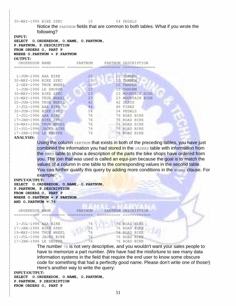
51
30-MAY-1996 BIKE SPEC 10 54 PEDALS
Notice the PARTNUM fields that are common to both tables. What if you wrote the following?
INPUT: SELECT O.ORDEREDON, O.NAME, O.PARTNUM,
P.PARTNUM, P.DESCRIPTION
FROM ORDERS O, PART P
WHERE O.PARTNUM = P.PARTNUM
OUTPUT: ORDEREDON NAME PARTNUM PARTNUM DESCRIPTION
=========== ========== =========== ========= ==============
1-JUN-1996 AAA BIKE 10 10 TANDEM
30-MAY-1996 BIKE SPEC 10 10 TANDEM
2-SEP-1996 TRUE WHEEL 10 10 TANDEM
1-JUN-1996 LE SHOPPE 10 10 TANDEM
30-MAY-1996 BIKE SPEC 23 23 MOUNTAIN BIKE
15-MAY-1996 TRUE WHEEL 23 23 MOUNTAIN BIKE
30-JUN-1996 TRUE WHEEL 42 42 SEATS
1-JUL-1996 AAA BIKE 46 46 TIRES
30-JUN-1996 BIKE SPEC 54 54 PEDALS
1-JUL-1996 AAA BIKE 76 76 ROAD BIKE
17-JAN-1996 BIKE SPEC 76 76 ROAD BIKE
19-MAY-1996 TRUE WHEEL 76 76 ROAD BIKE
11-JUL-1996 JACKS BIKE 76 76 ROAD BIKE
17-JAN-1996 LE SHOPPE 76 76 ROAD BIKE
ANALYSIS:
Using the column PARTNUM that exists in both of the preceding tables, you have just
combined the information you had stored in the ORDERS table with information from
the PART table to show a description of the parts the bike shops have ordered from you. The join that was used is called an equi-join because the goal is to match the values of a column in one table to the corresponding values in the second table.
You can further qualify this query by adding more conditions in the WHERE clause. For example:
INPUT/OUTPUT: SELECT O.ORDEREDON, O.NAME, O.PARTNUM,
P.PARTNUM, P.DESCRIPTION
FROM ORDERS O, PART P
WHERE O.PARTNUM = P.PARTNUM
AND O.PARTNUM = 76
ORDEREDON NAME PARTNUM PARTNUM DESCRIPTION
=========== ========== =========== ========== ============
1-JUL-1996 AAA BIKE 76 76 ROAD BIKE
17-JAN-1996 BIKE SPEC 76 76 ROAD BIKE
19-MAY-1996 TRUE WHEEL 76 76 ROAD BIKE
11-JUL-1996 JACKS BIKE 76 76 ROAD BIKE
17-JAN-1996 LE SHOPPE 76 76 ROAD BIKE
The number 76 is not very descriptive, and you wouldn't want your sales people to have to memorize a part number. (We have had the misfortune to see many data information systems in the field that require the end user to know some obscure code for something that had a perfectly good name. Please don't write one of those!) Here's another way to write the query:
INPUT/OUTPUT: SELECT O.ORDEREDON, O.NAME, O.PARTNUM,
P.PARTNUM, P.DESCRIPTION
FROM ORDERS O, PART P
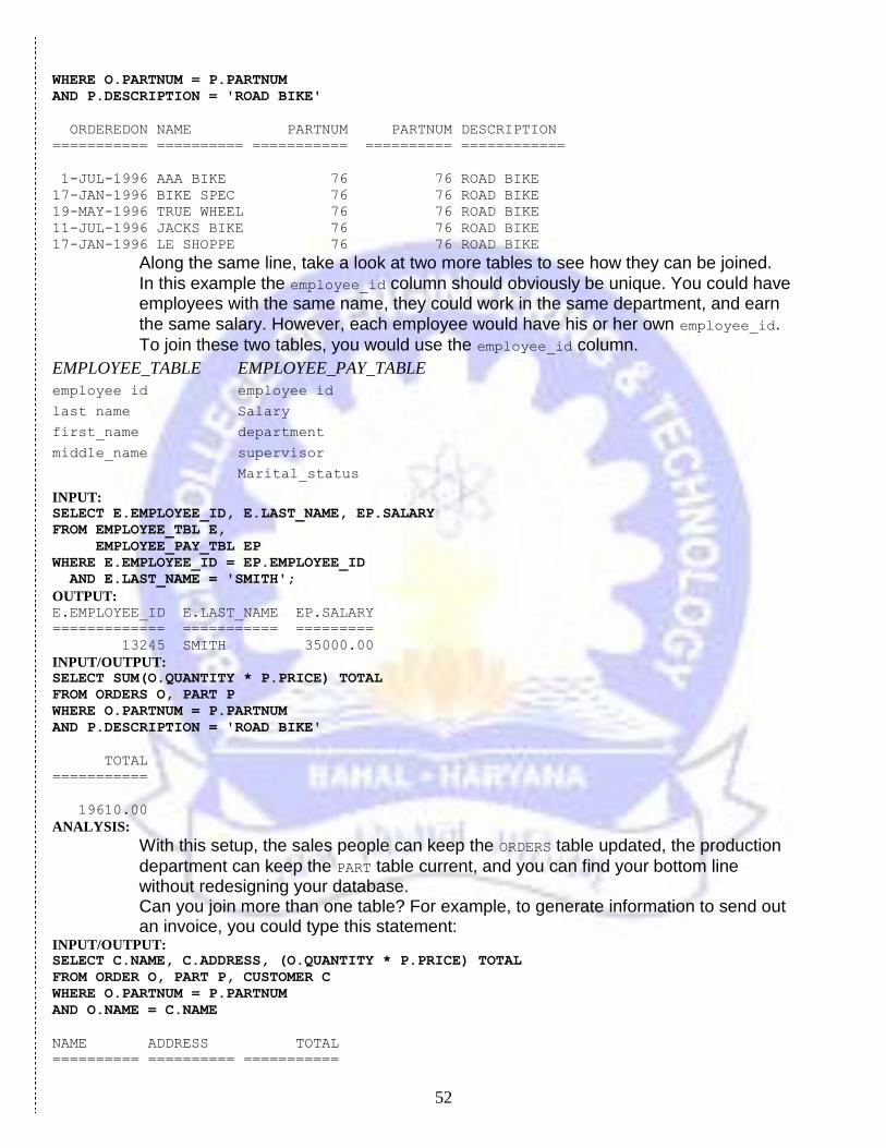
52
WHERE O.PARTNUM = P.PARTNUM
AND P.DESCRIPTION = 'ROAD BIKE'
ORDEREDON NAME PARTNUM PARTNUM DESCRIPTION
=========== ========== =========== ========== ============
1-JUL-1996 AAA BIKE 76 76 ROAD BIKE
17-JAN-1996 BIKE SPEC 76 76 ROAD BIKE
19-MAY-1996 TRUE WHEEL 76 76 ROAD BIKE
11-JUL-1996 JACKS BIKE 76 76 ROAD BIKE
17-JAN-1996 LE SHOPPE 76 76 ROAD BIKE
Along the same line, take a look at two more tables to see how they can be joined.
In this example the employee_id column should obviously be unique. You could have employees with the same name, they could work in the same department, and earn
the same salary. However, each employee would have his or her own employee_id.
To join these two tables, you would use the employee_id column.
EMPLOYEE_TABLE EMPLOYEE_PAY_TABLE
employee_id employee_id
last_name Salary
first_name department
middle_name supervisor
Marital_status
INPUT: SELECT E.EMPLOYEE_ID, E.LAST_NAME, EP.SALARY
FROM EMPLOYEE_TBL E,
EMPLOYEE_PAY_TBL EP
WHERE E.EMPLOYEE_ID = EP.EMPLOYEE_ID
AND E.LAST_NAME = 'SMITH';
OUTPUT: E.EMPLOYEE_ID E.LAST_NAME EP.SALARY
============= =========== =========
13245 SMITH 35000.00
INPUT/OUTPUT: SELECT SUM(O.QUANTITY * P.PRICE) TOTAL
FROM ORDERS O, PART P
WHERE O.PARTNUM = P.PARTNUM
AND P.DESCRIPTION = 'ROAD BIKE'
TOTAL
===========
19610.00
ANALYSIS:
With this setup, the sales people can keep the ORDERS table updated, the production
department can keep the PART table current, and you can find your bottom line without redesigning your database. Can you join more than one table? For example, to generate information to send out an invoice, you could type this statement:
INPUT/OUTPUT: SELECT C.NAME, C.ADDRESS, (O.QUANTITY * P.PRICE) TOTAL
FROM ORDER O, PART P, CUSTOMER C
WHERE O.PARTNUM = P.PARTNUM
AND O.NAME = C.NAME
NAME ADDRESS TOTAL
========== ========== ===========
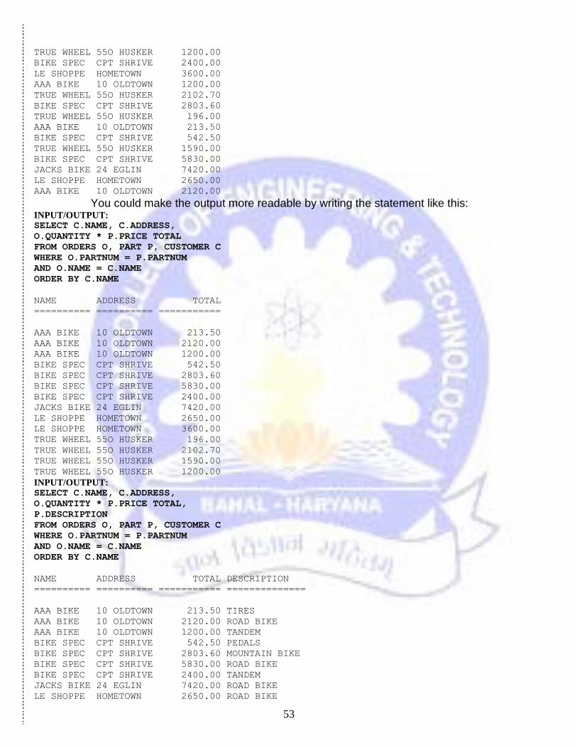
53
TRUE WHEEL 55O HUSKER 1200.00
BIKE SPEC CPT SHRIVE 2400.00
LE SHOPPE HOMETOWN 3600.00
AAA BIKE 10 OLDTOWN 1200.00
TRUE WHEEL 55O HUSKER 2102.70
BIKE SPEC CPT SHRIVE 2803.60
TRUE WHEEL 55O HUSKER 196.00
AAA BIKE 10 OLDTOWN 213.50
BIKE SPEC CPT SHRIVE 542.50
TRUE WHEEL 55O HUSKER 1590.00
BIKE SPEC CPT SHRIVE 5830.00
JACKS BIKE 24 EGLIN 7420.00
LE SHOPPE HOMETOWN 2650.00
AAA BIKE 10 OLDTOWN 2120.00
You could make the output more readable by writing the statement like this: INPUT/OUTPUT: SELECT C.NAME, C.ADDRESS,
O.QUANTITY * P.PRICE TOTAL
FROM ORDERS O, PART P, CUSTOMER C
WHERE O.PARTNUM = P.PARTNUM
AND O.NAME = C.NAME
ORDER BY C.NAME
NAME ADDRESS TOTAL
========== ========== ===========
AAA BIKE 10 OLDTOWN 213.50
AAA BIKE 10 OLDTOWN 2120.00
AAA BIKE 10 OLDTOWN 1200.00
BIKE SPEC CPT SHRIVE 542.50
BIKE SPEC CPT SHRIVE 2803.60
BIKE SPEC CPT SHRIVE 5830.00
BIKE SPEC CPT SHRIVE 2400.00
JACKS BIKE 24 EGLIN 7420.00
LE SHOPPE HOMETOWN 2650.00
LE SHOPPE HOMETOWN 3600.00
TRUE WHEEL 55O HUSKER 196.00
TRUE WHEEL 55O HUSKER 2102.70
TRUE WHEEL 55O HUSKER 1590.00
TRUE WHEEL 55O HUSKER 1200.00
INPUT/OUTPUT: SELECT C.NAME, C.ADDRESS,
O.QUANTITY * P.PRICE TOTAL,
P.DESCRIPTION
FROM ORDERS O, PART P, CUSTOMER C
WHERE O.PARTNUM = P.PARTNUM
AND O.NAME = C.NAME
ORDER BY C.NAME
NAME ADDRESS TOTAL DESCRIPTION
========== ========== =========== ==============
AAA BIKE 10 OLDTOWN 213.50 TIRES
AAA BIKE 10 OLDTOWN 2120.00 ROAD BIKE
AAA BIKE 10 OLDTOWN 1200.00 TANDEM
BIKE SPEC CPT SHRIVE 542.50 PEDALS
BIKE SPEC CPT SHRIVE 2803.60 MOUNTAIN BIKE
BIKE SPEC CPT SHRIVE 5830.00 ROAD BIKE
BIKE SPEC CPT SHRIVE 2400.00 TANDEM
JACKS BIKE 24 EGLIN 7420.00 ROAD BIKE
LE SHOPPE HOMETOWN 2650.00 ROAD BIKE
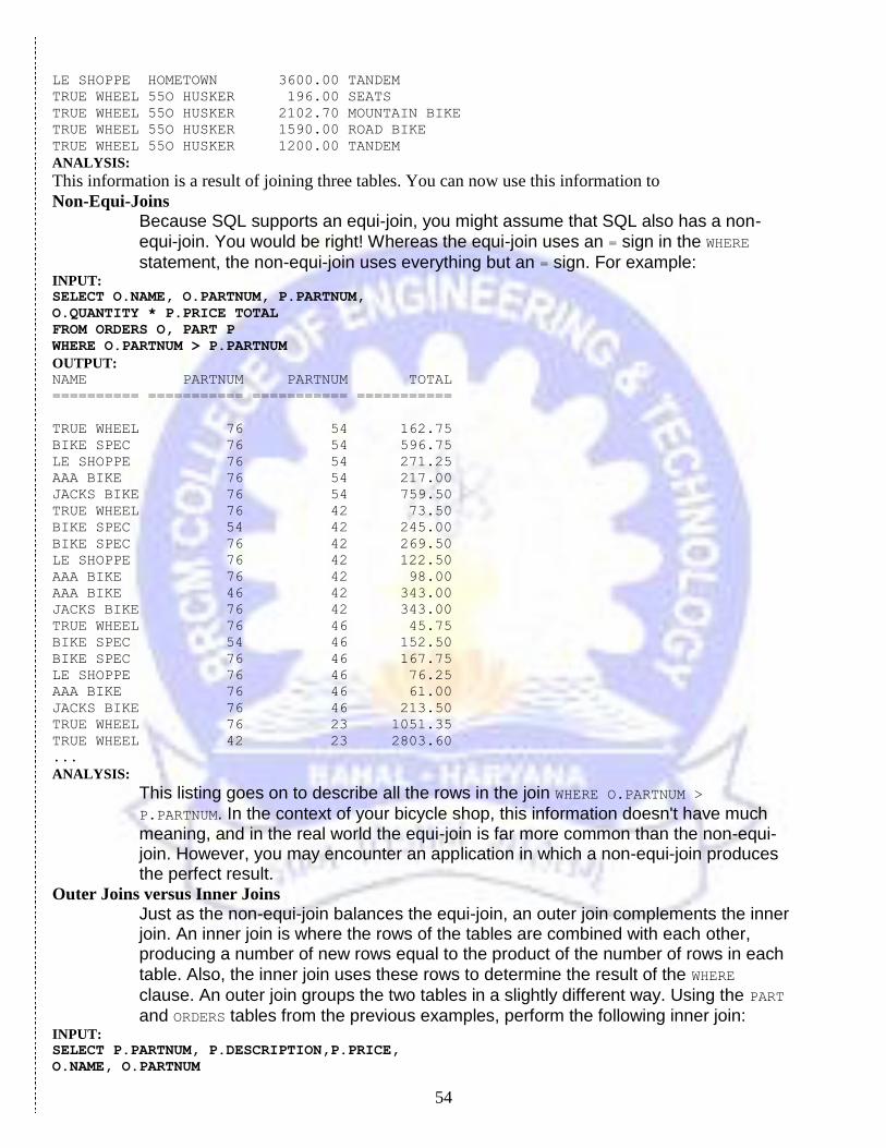
54
LE SHOPPE HOMETOWN 3600.00 TANDEM
TRUE WHEEL 55O HUSKER 196.00 SEATS
TRUE WHEEL 55O HUSKER 2102.70 MOUNTAIN BIKE
TRUE WHEEL 55O HUSKER 1590.00 ROAD BIKE
TRUE WHEEL 55O HUSKER 1200.00 TANDEM
ANALYSIS:
This information is a result of joining three tables. You can now use this information to
Non-Equi-Joins
Because SQL supports an equi-join, you might assume that SQL also has a non-
equi-join. You would be right! Whereas the equi-join uses an = sign in the WHERE
statement, the non-equi-join uses everything but an = sign. For example: INPUT: SELECT O.NAME, O.PARTNUM, P.PARTNUM,
O.QUANTITY * P.PRICE TOTAL
FROM ORDERS O, PART P
WHERE O.PARTNUM > P.PARTNUM
OUTPUT: NAME PARTNUM PARTNUM TOTAL
========== =========== =========== ===========
TRUE WHEEL 76 54 162.75
BIKE SPEC 76 54 596.75
LE SHOPPE 76 54 271.25
AAA BIKE 76 54 217.00
JACKS BIKE 76 54 759.50
TRUE WHEEL 76 42 73.50
BIKE SPEC 54 42 245.00
BIKE SPEC 76 42 269.50
LE SHOPPE 76 42 122.50
AAA BIKE 76 42 98.00
AAA BIKE 46 42 343.00
JACKS BIKE 76 42 343.00
TRUE WHEEL 76 46 45.75
BIKE SPEC 54 46 152.50
BIKE SPEC 76 46 167.75
LE SHOPPE 76 46 76.25
AAA BIKE 76 46 61.00
JACKS BIKE 76 46 213.50
TRUE WHEEL 76 23 1051.35
TRUE WHEEL 42 23 2803.60
...
ANALYSIS:
This listing goes on to describe all the rows in the join WHERE O.PARTNUM >
P.PARTNUM. In the context of your bicycle shop, this information doesn't have much meaning, and in the real world the equi-join is far more common than the non-equi-join. However, you may encounter an application in which a non-equi-join produces the perfect result.
Outer Joins versus Inner Joins
Just as the non-equi-join balances the equi-join, an outer join complements the inner join. An inner join is where the rows of the tables are combined with each other, producing a number of new rows equal to the product of the number of rows in each
table. Also, the inner join uses these rows to determine the result of the WHERE
clause. An outer join groups the two tables in a slightly different way. Using the PART
and ORDERS tables from the previous examples, perform the following inner join: INPUT: SELECT P.PARTNUM, P.DESCRIPTION,P.PRICE,
O.NAME, O.PARTNUM
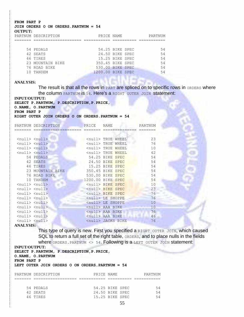
55
FROM PART P
JOIN ORDERS O ON ORDERS.PARTNUM = 54
OUTPUT: PARTNUM DESCRIPTION PRICE NAME PARTNUM
======= ==================== =========== ========== ===========
54 PEDALS 54.25 BIKE SPEC 54
42 SEATS 24.50 BIKE SPEC 54
46 TIRES 15.25 BIKE SPEC 54
23 MOUNTAIN BIKE 350.45 BIKE SPEC 54
76 ROAD BIKE 530.00 BIKE SPEC 54
10 TANDEM 1200.00 BIKE SPEC 54
ANALYSIS:
The result is that all the rows in PART are spliced on to specific rows in ORDERS where
the column PARTNUM is 54. Here's a RIGHT OUTER JOIN statement: INPUT/OUTPUT: SELECT P.PARTNUM, P.DESCRIPTION,P.PRICE,
O.NAME, O.PARTNUM
FROM PART P
RIGHT OUTER JOIN ORDERS O ON ORDERS.PARTNUM = 54
PARTNUM DESCRIPTION PRICE NAME PARTNUM
======= ==================== ======= ============== =======
<null> <null> <null> TRUE WHEEL 23
<null> <null> <null> TRUE WHEEL 76
<null> <null> <null> TRUE WHEEL 10
<null> <null> <null> TRUE WHEEL 42
54 PEDALS 54.25 BIKE SPEC 54
42 SEATS 24.50 BIKE SPEC 54
46 TIRES 15.25 BIKE SPEC 54
23 MOUNTAIN BIKE 350.45 BIKE SPEC 54
76 ROAD BIKE 530.00 BIKE SPEC 54
10 TANDEM 1200.00 BIKE SPEC 54
<null> <null> <null> BIKE SPEC 10
<null> <null> <null> BIKE SPEC 23
<null> <null> <null> BIKE SPEC 76
<null> <null> <null> LE SHOPPE 76
<null> <null> <null> LE SHOPPE 10
<null> <null> <null> AAA BIKE 10
<null> <null> <null> AAA BIKE 76
<null> <null> <null> AAA BIKE 46
<null> <null> <null> JACKS BIKE 76
ANALYSIS:
This type of query is new. First you specified a RIGHT OUTER JOIN, which caused
SQL to return a full set of the right table, ORDERS, and to place nulls in the fields
where ORDERS.PARTNUM <> 54. Following is a LEFT OUTER JOIN statement: INPUT/OUTPUT: SELECT P.PARTNUM, P.DESCRIPTION,P.PRICE,
O.NAME, O.PARTNUM
FROM PART P
LEFT OUTER JOIN ORDERS O ON ORDERS.PARTNUM = 54
PARTNUM DESCRIPTION PRICE NAME PARTNUM
======= ================== =========== ========== ===========
54 PEDALS 54.25 BIKE SPEC 54
42 SEATS 24.50 BIKE SPEC 54
46 TIRES 15.25 BIKE SPEC 54
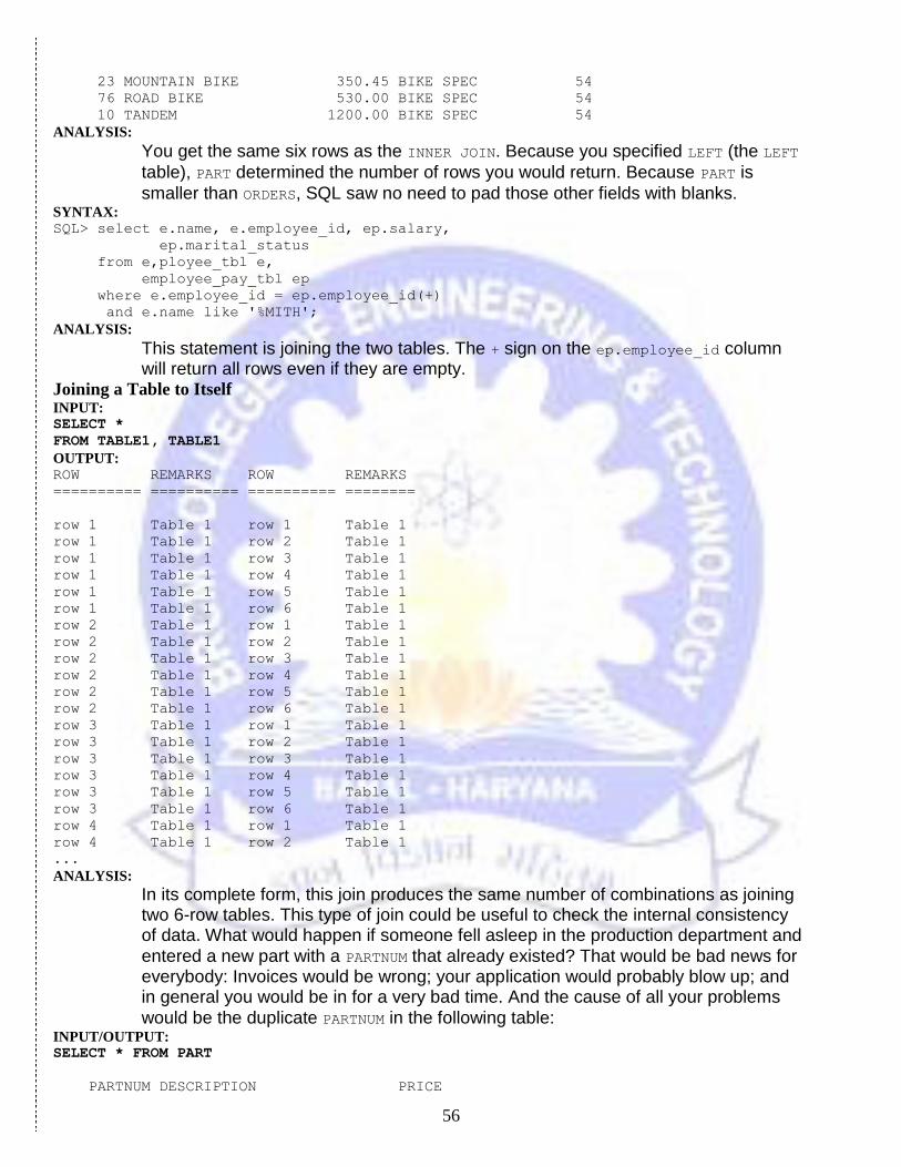
56
23 MOUNTAIN BIKE 350.45 BIKE SPEC 54
76 ROAD BIKE 530.00 BIKE SPEC 54
10 TANDEM 1200.00 BIKE SPEC 54
ANALYSIS:
You get the same six rows as the INNER JOIN. Because you specified LEFT (the LEFT
table), PART determined the number of rows you would return. Because PART is
smaller than ORDERS, SQL saw no need to pad those other fields with blanks. SYNTAX: SQL> select e.name, e.employee_id, ep.salary,
ep.marital_status
from e,ployee_tbl e,
employee_pay_tbl ep
where e.employee_id = ep.employee_id(+)
and e.name like '%MITH';
ANALYSIS:
This statement is joining the two tables. The + sign on the ep.employee_id column will return all rows even if they are empty.
Joining a Table to Itself INPUT: SELECT *
FROM TABLE1, TABLE1
OUTPUT: ROW REMARKS ROW REMARKS
========== ========== ========== ========
row 1 Table 1 row 1 Table 1
row 1 Table 1 row 2 Table 1
row 1 Table 1 row 3 Table 1
row 1 Table 1 row 4 Table 1
row 1 Table 1 row 5 Table 1
row 1 Table 1 row 6 Table 1
row 2 Table 1 row 1 Table 1
row 2 Table 1 row 2 Table 1
row 2 Table 1 row 3 Table 1
row 2 Table 1 row 4 Table 1
row 2 Table 1 row 5 Table 1
row 2 Table 1 row 6 Table 1
row 3 Table 1 row 1 Table 1
row 3 Table 1 row 2 Table 1
row 3 Table 1 row 3 Table 1
row 3 Table 1 row 4 Table 1
row 3 Table 1 row 5 Table 1
row 3 Table 1 row 6 Table 1
row 4 Table 1 row 1 Table 1
row 4 Table 1 row 2 Table 1
...
ANALYSIS:
In its complete form, this join produces the same number of combinations as joining two 6-row tables. This type of join could be useful to check the internal consistency of data. What would happen if someone fell asleep in the production department and
entered a new part with a PARTNUM that already existed? That would be bad news for everybody: Invoices would be wrong; your application would probably blow up; and in general you would be in for a very bad time. And the cause of all your problems
would be the duplicate PARTNUM in the following table: INPUT/OUTPUT: SELECT * FROM PART
PARTNUM DESCRIPTION PRICE
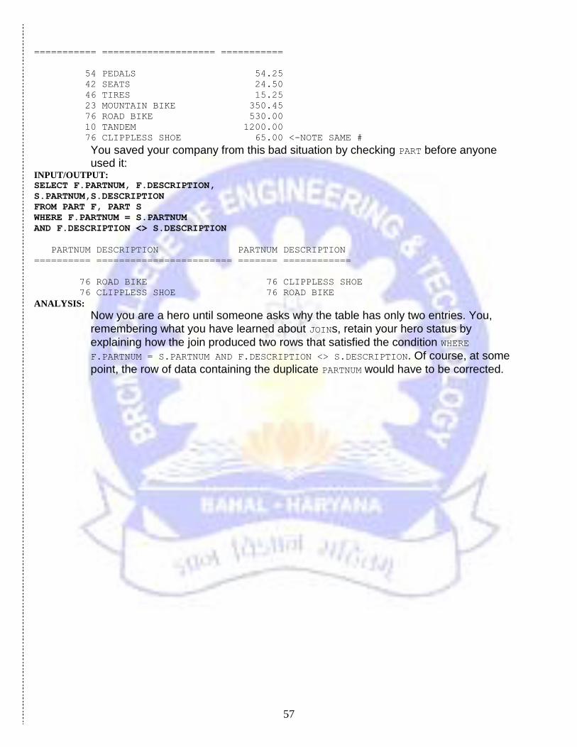
57
=========== ==================== ===========
54 PEDALS 54.25
42 SEATS 24.50
46 TIRES 15.25
23 MOUNTAIN BIKE 350.45
76 ROAD BIKE 530.00
10 TANDEM 1200.00
76 CLIPPLESS SHOE 65.00 <-NOTE SAME #
You saved your company from this bad situation by checking PART before anyone used it:
INPUT/OUTPUT: SELECT F.PARTNUM, F.DESCRIPTION,
S.PARTNUM,S.DESCRIPTION
FROM PART F, PART S
WHERE F.PARTNUM = S.PARTNUM
AND F.DESCRIPTION <> S.DESCRIPTION
PARTNUM DESCRIPTION PARTNUM DESCRIPTION
========== ======================== ======= ============
76 ROAD BIKE 76 CLIPPLESS SHOE
76 CLIPPLESS SHOE 76 ROAD BIKE
ANALYSIS:
Now you are a hero until someone asks why the table has only two entries. You,
remembering what you have learned about JOINs, retain your hero status by
explaining how the join produced two rows that satisfied the condition WHERE
F.PARTNUM = S.PARTNUM AND F.DESCRIPTION <> S.DESCRIPTION. Of course, at some
point, the row of data containing the duplicate PARTNUM would have to be corrected.