THE CONFORMAL GEOMETRY OF BILLIARDS

LAURA DE MARCO

In the absence of friction and other external forces, a billiard ball on a rectangular

billiard table follows a predictable path. As it reflects off the sides of the table, the

ball will either (1) return to its original position and direction, or (2) travel all over the

table, spending equal time in regions with equal area. Because of this dichotomy, we

say the rectangular table is optimal: billiard trajectories define an easily understood

dynamical system on the phase space of positions and directions.

In this article, we ask:

Which polygonal shapes make optimal billiard tables?

Our primary goal is to tell a story about billiards which provides an entry point

to a large and active area of research. We will explore some recent results on the

search for, and the classification of, the optimal billiard tables. We will also discuss

some general results about the Teichmuller geometry of the moduli space of Riemann

surfaces and its connection with billiard dynamical systems.

We concentrate on the billiard dynamics in polygons T ⊂ R2 with all interior angles

equal to rational multiples of π. Each such billiard table gives rise to

• a compact translation surface, that is, a pair (X,ω) consisting of a compact

Riemann surface X and a holomorphic 1-form ω on X, via a process called

unfolding; and

• a discrete group of 2-by-2 matrices SL(X,ω) ⊂ SL2R, consisting of the linear

parts of affine automorphisms of the surface (X, ω).

The path of a billiard ball, which bounces around the table by reflecting off the sides,

unfolds into a straight line on the surface X, with respect to the Euclidean metric

determined by ω. Thus, the study of billiard dynamics on a table becomes the study

of the geodesic flow on (X, |ω|). The structure of the group SL(X, ω) will determine

properties of the geodesic flow.

We will introduce three types of optimal billiard tables; namely, the lattice poly-

gons, the ergodically optimal tables, and the topologically optimal tables. Of the

three, the lattice polygon is the most restrictive type. By definition, the billiard table

T is a lattice polygon if SL(X, ω) forms a lattice in SL2R; this means that the quotient

SL2R/SL(X, ω) has finite volume. Traditional rectangular tables and the pentagon

of Figure 1 are examples.

Date: October 18, 2010.

2 LAURA DE MARCO

Figure 1. A billiard trajectory on the regular pentagon.

The ergodically optimal and topologically optimal tables are defined purely in terms

of their billiard dynamical systems. On an ergodically optimal table, any billiard tra-

jectory (which avoids the corners) is either periodic or uniformly distributed, while

topologically optimal tables satisfy a weaker dichotomy: trajectories are either peri-

odic or dense. Lattice polygons are both ergodically and topologically optimal, but a

characterization of lattice polygons only in terms of their billiard dynamics remains

open.

There is an additional dynamical system, an action of SL2R on the moduli space

ΩMg of all compact translation surfaces of genus g. When the surface (X, ω) arises

from a billiard table T , it is remarkable that properties of its orbit under the SL2Raction determine properties of the original billiard dynamical system on T . In fact,

the group SL(X, ω), defined by symmetries of (X, ω), coincides with the stabilizer of

(X,ω) under this SL2R action. The question of which shapes make optimal billiard

tables thus broadens into questions about global invariants of this action on the

moduli space.

We will see a few of the general results about this SL2R action on ΩMg, but we

will keep billiard dynamics as the main focus of this article. We give no proofs, but

we provide references throughout.

Acknowledgements. I am greatly indebted to the experts in translation surfaces for

helping me prepare this article. Special thanks go to Yitwah Cheung, Howard Masur,

and Curt McMullen for lengthy conversations and numerous email exchanges. Curt

McMullen generated the images of Figures 1 and 3. I would also like to thank Jayadev

Athreya, Matt Bainbridge, Alex Eskin, Pat Hooper, Chris Judge, Ben McReynolds,

and John Smillie for helpful discussions. This article does not do justice to their

beautiful results; the emphasis here reflects my own bias and background.

THE CONFORMAL GEOMETRY OF BILLIARDS 3

This article is an expanded version of my notes for the Current Events session at

the January 2010 meeting of the American Mathematical Society in San Francisco.

I thank the AMS and David Eisenbud for inviting me to learn about billiards. My

research is supported by the National Science Foundation and the Sloan Foundation.

Contents

1. Billiard tables and optimal dynamics 4

1.1. The square table 4

1.2. Ergodically optimal billiard dynamics 4

1.3. First examples and non-examples 5

1.4. Dense but non-uniformly distributed trajectories 6

1.5. Topologically optimal billiard tables 7

2. The translation surface of a billiard table 7

2.1. Translation structure on a Riemann surface 7

2.2. Unfolding a billiard table into a translation surface 8

2.3. Surfaces from tables, but not vice versa 9

2.4. Geodesic flow on a translation surface 9

2.5. The affine group of symmetries and its linear part 9

2.6. Lattice polygons and surfaces 9

3. An SL2R action on moduli space 10

3.1. Stretching the Euclidean coordinates 10

3.2. The moduli space of translation surfaces 11

3.3. Teichmuller geometry and Teichmuller curves 11

3.4. Masur’s theorem and the Veech dichotomy 12

3.5. Genus 1 13

3.6. Genus 2 and geometric primitivity 13

3.7. Higher genus and algebraic primitivity 14

3.8. Invariant measures and orbit closures 15

4. Towards a characterization of optimal dynamics or the lattice condition 15

4.1. Characterization in genus 2 15

4.2. Coverings and branched coverings 17

4.3. The triangle of Theorem 1.3 18

4.4. Possible characterization of the lattice condition: rational ratios of

moduli 18

5. Examples of groups SL(X, ω) and the search for optimal billiard tables 19

5.1. Arithmetic groups 19

5.2. Triangle groups 19

5.3. Infinitely generated groups 20

4 LAURA DE MARCO

5.4. Triangles and the continued search 21

References 22

1. Billiard tables and optimal dynamics

For this article, a billiard table means a connected polygon in R2 with all angles

equal to rational multiples of π. A billiard trajectory in direction θ is a straight-line

path which begins at some point in the interior of the table, at angle θ as measured

from the positive real axis, and bounces off the edges with angle of reflection equal

to the angle of incidence. As the angles are rational multiples of π, the billiard path

will travel again in direction θ after finitely many reflections off the sides of the table.

If a billiard trajectory hits a vertex of the polygon, it stops. See Figure 2.

In this section, we define two notions of optimal billiard dynamics: ergodically

optimal and topologically optimal.

1.1. The square table. The simplest example is the square table of side length 1,

with sides parallel to the coordinate axes. In this table, it is easy to see that any

billiard trajectory of rational slope will either hit a vertex or eventually return to

its original configuration (position and angle). On the other hand, for all irrational

slopes and any initial point, a trajectory will either encounter a vertex or it will

bounce around the table spending equal time in parts with equal area. In particular,

the closure of any infinite trajectory with irrational slope will be the whole table.

1.2. Ergodically optimal billiard dynamics. We say a billiard table is ergodically

optimal if for each direction θ, one of the following holds:

(1) every trajectory that avoids the vertices is periodic; or

(2) every trajectory that avoids the vertices is uniformly distributed.

Figure 2. Polygonal billiard tables and trajectories.

THE CONFORMAL GEOMETRY OF BILLIARDS 5

We must take care in our meaning of uniform distribution: the trajectory determines

a closed, invariant surface in the phase space (of all possible positions and directions),

and the trajectory must spend equal time in regions of the surface with equal area.

To make this more precise, note that every trajectory points in only finitely many

different directions under reflections off the sides of the tables, because all angles

are rational multiples of π. For each direction θ, we take multiple copies of the

polygonal table, one for each direction arising by reflection of trajectories in direction

θ. For any trajectory of infinite length that starts in direction θ, let γ(t), t ≥ 0,

be a parametrization of this trajectory with unit speed (so with each reflection in a

side, γ(t) jumps to another copy of the table). For each time s > 0, we can define a

probability measure on the union of tables by

1

sγ∗ms

where ms is arc-length measure on the interval [0, s] in R. Uniform distribution means

that this family of measures converges weakly as s →∞ to normalized area measure

on the finite union of polygonal tables.

The property of ergodically optimal dynamics is also called Veech dichotomy in the

literature. The uniform distribution of all (infinite) trajectories in some direction is

called unique ergodicity.

1.3. First examples and non-examples. As explained in §1.1, the unit square

table is ergodically optimal. By similar reasoning, any rectangular table will be

ergodically optimal. With more work, it is also possible to show:

Theorem 1.1. [Gu] Any billiard table which is tiled by squares is ergodically optimal.

A tiling by squares requires that all tiles be translates of a single square, and all

vertices of the polygon lie on vertices of the tiles. Using different methods, Veech

showed:

Theorem 1.2. [Ve] For every n ≥ 3, the regular n-gon is ergodically optimal.

On the other hand, it is easy to construct tables which are not ergodically optimal.

For example, begin with a square table and attach a rectangle to one side with side

lengths a and b where a/b 6∈ Q. See Figure 3. Taking the direction θ = π/4, we

see that the trajectories in direction θ which enter the smaller rectangle are neither

closed nor dense.

We shall see many more ergodically optimal examples throughout this article. In

Section 3, we relate this dynamical property of being ergodically optimal to the

Teichmuller geometry of moduli space and the stronger condition of being a lattice

polygon.

6 LAURA DE MARCO

Figure 3. A billiard trajectory on an L-shaped table, neither closed

nor dense.

!

1

2

Figure 4. A rectangular billiard table with barrier of length `.

1.4. Dense but non-uniformly distributed trajectories. It is a non-trivial task

to find billiard trajectories which are dense but non-uniformly distributed, but they

do exist. The following examples were studied by Masur and Smillie, following a

construction of Veech; see the discussion in [MT, §3.1]. Consider a rectangular table

with barrier as in Figure 4: begin with a rectangular table of side lengths 1 and 2

and build a perpendicular wall in the middle of the long side of length ` < 1. When

` is rational, the table is ergodically optimal. When ` is irrational, there are orbits

which are neither dense nor closed (as for the trajectory of Figure 3), and there are

dense orbits that are non-uniformly distributed. In fact, when ` is Diophantine (so

it is not too closely approximated by rationals), the set of directions θ ∈ [0, 2π)

with dense but non-uniformly distributed trajectories is as large as possible, having

Hausdorff dimension 1/2 [Ch]. In the recent preprint [CHM2], the authors provide an

arithmetic condition on the barrier length ` that characterizes the tables with a large

set of minimal, non-uniquely ergodic directions. Minimal means that all (infinite)

trajectories in the given direction are dense.

THE CONFORMAL GEOMETRY OF BILLIARDS 7

3!/103!/10

2!/5

Figure 5. A triangular table with topologically optimal dynamics but

not ergodically optimal; there are dense trajectories that are not uni-

formly distributed.

1.5. Topologically optimal billiard tables. A billiard table is said to be topolog-

ically optimal if for each direction θ,

(1) every trajectory that avoids the vertices is periodic; or

(2) every trajectory that avoids the vertices is dense.

As with uniform distribution, we require that the trajectory be dense on the finite

union of tables corresponding to different directions under reflection.

Ergodically optimal clearly implies topologically optimal. The following recent

result shows that the converse is not true:

Theorem 1.3. [CHM1] The billiard dynamics on the isosceles triangle with angles

(2π/5, 3π/10, 3π/10) are topologically optimal but not ergodically optimal: for each

direction, either all infinite trajectories are closed or all are dense, but there exist

trajectories which are dense but not uniformly distributed.

See Figure 5. In standard dynamical language, the billiard flow in each direction

is either completely periodic or minimal, while certain minimal directions are not

uniquely ergodic. In fact, this is the only known billiard table to be topologically

optimal but not ergodically optimal. More will be said about this example in §4.3.

2. The translation surface of a billiard table

In this section we describe the process of unfolding, i.e. passing from a polygonal

billiard table to a Riemann surface equipped with a holomorphic 1-form. In this way,

a billiard trajectory which reflects off the sides of the table unfolds into a straight

line on the surface. We also define the symmetry group SL(X, ω) associated to any

translation surface. We extend the notions of ergodically optimal and topologically

optimal (from Section 1) to general translation surfaces. Finally, we introduce the

notion of a lattice surface and compare it to an ergodically optimal surface.

2.1. Translation structure on a Riemann surface. By definition, a holomorphic

1-form ω on a Riemann surface X can be expressed in local coordinates as

ω = f(z) dz

8 LAURA DE MARCO

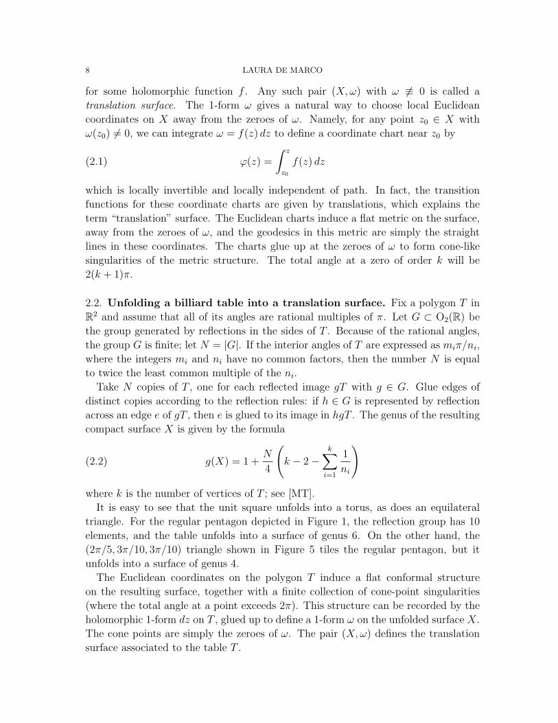
for some holomorphic function f . Any such pair (X, ω) with ω 6≡ 0 is called a

translation surface. The 1-form ω gives a natural way to choose local Euclidean

coordinates on X away from the zeroes of ω. Namely, for any point z0 ∈ X with

ω(z0) 6= 0, we can integrate ω = f(z) dz to define a coordinate chart near z0 by

(2.1) ϕ(z) =

∫ z

z0

f(z) dz

which is locally invertible and locally independent of path. In fact, the transition

functions for these coordinate charts are given by translations, which explains the

term “translation” surface. The Euclidean charts induce a flat metric on the surface,

away from the zeroes of ω, and the geodesics in this metric are simply the straight

lines in these coordinates. The charts glue up at the zeroes of ω to form cone-like

singularities of the metric structure. The total angle at a zero of order k will be

2(k + 1)π.

2.2. Unfolding a billiard table into a translation surface. Fix a polygon T in

R2 and assume that all of its angles are rational multiples of π. Let G ⊂ O2(R) be

the group generated by reflections in the sides of T . Because of the rational angles,

the group G is finite; let N = |G|. If the interior angles of T are expressed as miπ/ni,

where the integers mi and ni have no common factors, then the number N is equal

to twice the least common multiple of the ni.

Take N copies of T , one for each reflected image gT with g ∈ G. Glue edges of

distinct copies according to the reflection rules: if h ∈ G is represented by reflection

across an edge e of gT , then e is glued to its image in hgT . The genus of the resulting

compact surface X is given by the formula

(2.2) g(X) = 1 +N

4

(k − 2−

k∑i=1

1

ni

)where k is the number of vertices of T ; see [MT].

It is easy to see that the unit square unfolds into a torus, as does an equilateral

triangle. For the regular pentagon depicted in Figure 1, the reflection group has 10

elements, and the table unfolds into a surface of genus 6. On the other hand, the

(2π/5, 3π/10, 3π/10) triangle shown in Figure 5 tiles the regular pentagon, but it

unfolds into a surface of genus 4.

The Euclidean coordinates on the polygon T induce a flat conformal structure

on the resulting surface, together with a finite collection of cone-point singularities

(where the total angle at a point exceeds 2π). This structure can be recorded by the

holomorphic 1-form dz on T , glued up to define a 1-form ω on the unfolded surface X.

The cone points are simply the zeroes of ω. The pair (X, ω) defines the translation

surface associated to the table T .

THE CONFORMAL GEOMETRY OF BILLIARDS 9

2.3. Surfaces from tables, but not vice versa. Every translation surface (X,ω)

with X compact can be obtained by gluing a finite collection of polygons, via transla-

tions in the plane, taking the 1-form dz on the each of the polygons; see the discussion

in [Ma2]. In general, though, the polygons will not be reflections of a single polygonal

shape T . In any given genus, the subset of billiard table surfaces within the space of

all translation surfaces (X, ω) forms a small (measure 0) subset.

2.4. Geodesic flow on a translation surface. The notion of optimal dynamics

can be defined on general translation surfaces (X, ω), in the context of the geodesic

flow. Specifically, given a point x ∈ X with ω(x) 6= 0 and a vector v of unit length in

the tangent space at x, the image of x under the time t geodesic flow is the unique

point at distance t from x in direction v. The flow is only well-defined where straight

lines avoid the zeroes of ω. We say a translation surface (X, ω) is ergodically optimal if

its geodesics satisfy the dichotomy of §1.2. We say the surface is topologically optimal

if its geodesics satisfy the weaker dichotomy of §1.5.

The idea of unfolding seems to have first appeared in [KZ], where the authors

studied topological transitivity of the geodesic flow on the associated translation

surface, concluding that most directions on a table are minimal (so that all trajectories

avoiding the corners of the table are dense). General results about differentials on

closed surfaces imply that there exist periodic trajectories in a dense set of directions;

see [MT]. On the other hand, it is known that almost every direction gives rise to

uniformly distributed geodesics on a translation surface [KMS].

2.5. The affine group of symmetries and its linear part. Fix a compact trans-

lation surface (X, ω). An orientation-preserving diffeomorphism h : X → X is an

affine automorphism if it is affine in the local Euclidean coordinates from ω. Because

h must preserve area and orientation, its linear part (i.e. its derivative Dh) is a 2

by 2 matrix of determinant 1. We let SL(X,ω) ⊂ SL2R denote the group of linear

parts, formed from all affine automorphisms of (X, ω). The group SL(X, ω) is always

a discrete subgroup of SL2R.

2.6. Lattice polygons and surfaces. It can happen that SL(X, ω) forms a lattice

in SL2R, meaning that the quotient SL2R/SL(X, ω) has finite volume. In this case,

we say the surface (X, ω) is a lattice surface. When a billiard table T unfolds into a

lattice surface, we say that T is a lattice polygon. As an example, the group SL(X,ω)

for the unfolding of the square table is the lattice SL2Z, consisting of all 2×2 matrices

with integer entries and determinant 1. In fact, the square-tiled tables of Theorem

1.1 are all lattice polygons. In general, we have:

Theorem 2.1. [Ve] If SL(X, ω) ⊂ SL2R is a lattice, then (X, ω) is ergodically opti-

mal.

10 LAURA DE MARCO

In §3.4, we will sketch the proof of this result. By computing the group SL(X, ω)

explicitly for the translation surface associated to a regular n-gon billiard table, Veech

used this Theorem 2.1 to deduce Theorem 1.2.

Only recently, Smillie and Weiss have shown that the converse of Theorem 2.1 does

not hold:

Theorem 2.2. [SW] There exist translation surfaces (X, ω) which are ergodically

optimal but for which SL(X,ω) is not a lattice.

More will be said about this theorem in §4.2.

In the following section, we will explore some of the ideas which enter into the

search for lattice surfaces and their relation to the Teichmuller geometry of moduli

space.

3. An SL2R action on moduli space

In this section, we describe a linear stretching action on the space of translation

surfaces. We introduce Teichmuller curves, algebraic curves in the moduli space Mg

of genus g compact Riemann surfaces which are isometrically immersed with respect

to the Teichmuller metric. The translation surfaces (X, ω) which generate Teichmuller

curves are precisely the lattice surfaces, introduced in §2.6. We describe McMullen’s

classification of Teichmuller curves in genus 2, and we mention a few results about

the search for Teichmuller curves in higher genus. We conclude with a description of

the main goal in this direction of study: a complete analysis of orbits and invariant

measures for the action of SL2R on the moduli space ΩMg.

3.1. Stretching the Euclidean coordinates. Fix a translation surface (X, ω). We

can define a new translation surface A · (X, ω) for each A ∈ SL2R by composing the

natural Euclidean charts for ω with A. Specifically, recall that charts for X are defined

by the ϕ of equation (2.1) away from the zeroes of ω. We replace each such ϕ with

A ϕ. These charts A ϕ glue to form a new Riemann surface Y , homeomorphic

to X, and the 1-form dz in the plane defines a holomorphic 1-form η on Y . We set

A · (X, ω) = (Y, η).

In the context of billiard tables, the action may be viewed as follows. Apply the

matrix A to the billiard table T and each of its reflected copies to obtain a new

collection of polygons. Maintain the identification of edges that form the unfolded

surface for T , and glue corresponding pairs of edges of the stretched polygons by

translations. See Figure 6.

Recall that every translation surface (X,ω) can be represented by a finite set of

polygons Pi in the plane, with edges identified by translations. The new surface

A·(X,ω) can be viewed as the set of polygons A(Pi) with edges identified according

to the same combinatorial rules.

THE CONFORMAL GEOMETRY OF BILLIARDS 11

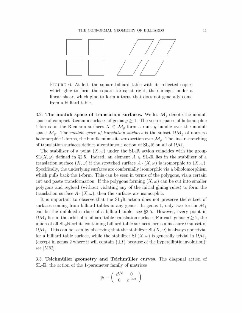
Figure 6. At left, the square billiard table with its reflected copies

which glue to form the square torus; at right, their images under a

linear shear, which glue to form a torus that does not generally come

from a billiard table.

3.2. The moduli space of translation surfaces. We let Mg denote the moduli

space of compact Riemann surfaces of genus g ≥ 1. The vector spaces of holomorphic

1-forms on the Riemann surfaces X ∈ Mg form a rank g bundle over the moduli

space Mg. The moduli space of translation surfaces is the subset ΩMg of nonzero

holomorphic 1-forms, the bundle minus its zero section overMg. The linear stretching

of translation surfaces defines a continuous action of SL2R on all of ΩMg.

The stabilizer of a point (X, ω) under the SL2R action coincides with the group

SL(X, ω) defined in §2.5. Indeed, an element A ∈ SL2R lies in the stabilizer of a

translation surface (X, ω) if the stretched surface A · (X, ω) is isomorphic to (X, ω).

Specifically, the underlying surfaces are conformally isomorphic via a biholomorphism

which pulls back the 1-form. This can be seen in terms of the polygons, via a certain

cut and paste transformation. If the polygons forming (X, ω) can be cut into smaller

polygons and reglued (without violating any of the initial gluing rules) to form the

translation surface A · (X, ω), then the surfaces are isomorphic.

It is important to observe that the SL2R action does not preserve the subset of

surfaces coming from billiard tables in any genus. In genus 1, only two tori in M1

can be the unfolded surface of a billiard table; see §3.5. However, every point in

ΩM1 lies in the orbit of a billiard table translation surface. For each genus g ≥ 2, the

union of all SL2R-orbits containing billiard table surfaces forms a measure 0 subset of

ΩMg. This can be seen by observing that the stabilizer SL(X, ω) is always nontrivial

for a billiard table surface, while the stabilizer SL(X, ω) is generally trivial in ΩMg

(except in genus 2 where it will contain ±I because of the hyperelliptic involution);

see [Mo2].

3.3. Teichmuller geometry and Teichmuller curves. The diagonal action of

SL2R, the action of the 1-parameter family of matrices

gt =

(et/2 0

0 e−t/2

)

12 LAURA DE MARCO

on the space of translation surfaces ΩMg, plays a key role. It parametrizes the

Teichmuller geodesic flow on the moduli space Mg. Via these flow lines, a 1-form ω

on X gives rise to a tangent vector to X ∈ Mg; its norm in the Teichmuller metric

is the integral ∫X

|ω|2.

See [Hu, Chapter 6] for background on Teichmuller spaces and the Teichmuller metric.

Recall that the quotient SO2R\SL2R can be naturally identified with the hyperbolic

plane H. For a given translation surface (X, ω), the rotations preserve the underlying

surface X, and the orbit

SL2R 3 A 7→ A · (X, ω) ∈ ΩMg

descends to a holomorphic map

H →Mg

which is a local isometry with respect to the Poincare metric on the upper half-plane Hand the Teichmuller metric on Mg; see e.g. [KMS], [Ve], [Mc1]. When the stabilizer

SL(X, ω) forms a lattice, the image of H forms an algebraic curve in Mg. Such

curves are called Teichmuller curves; these are precisely the isometrically embedded

algebraic curves in Mg. Recall that each Teichmuller curve gives rise to a family of

ergodically optimal translation surfaces, by Theorem 2.1. Using this lattice condition

to locate ergodically optimal surfaces, we see how an understanding of Teichmuller

geometry of Mg, in addition to the properties of this SL2R action, might help us

classify such surfaces and ergodically optimal billiard tables.

3.4. Masur’s theorem and the Veech dichotomy. In Theorem 2.1, we have seen

that any surface with SL(X, ω) a lattice will be ergodically optimal. The proof of this

result follows from a theorem of Masur:

Theorem 3.1. [Ma1] If the orbit gt · (X,ω) is recurrent in Mg, then the vertical

direction on (X, ω) is uniquely ergodic.

Recall that a direction is uniquely ergodic if it satisfies condition (2) in the ergodically

optimal dichotomy of §1.2. The vertical trajectories are those in direction θ = π/2

with respect to the natural Euclidean coordinates on (X, ω). As described in §3.3,

the image of gt · (X, ω) in Mg is a geodesic in the Teichmuller metric.

Any geodesic on a Teichmuller curve is either recurrent or it heads out a cusp. In

the first case, the direction is uniquely ergodic by Theorem 3.1. Veech’s Theorem 2.1

follows by analyzing the case where a geodesic goes out the cusp. In that case, the

geodesic gt ·(X, ω) must be orthogonal to a closed horocycle on the Teichmuller curve.

There is then a parabolic element of SL(X, ω) which preserves the vertical foliation,

acting as the identity on leaves connecting zeroes. These closed leaves decompose the

surface (X, ω) into cylinders. See details in [Ma2].

THE CONFORMAL GEOMETRY OF BILLIARDS 13

3.5. Genus 1. There is a unique holomorphic 1-form (up to scaling) on a torus,

coming from the form dz on C, when representing the torus as the quotient of C by a

lattice. The translation structure from dz is just the usual flat metric from the plane

with no singularities. It is well-known that geodesics on a flat torus satisfy the optimal

dichotomy described in §1.2. As there are no zeroes of the 1-form, every geodesic is

infinite; so in a given direction, all are closed or all are dense. Thus any billiard

table which unfolds into a genus 1 translation surface must be ergodically optimal.

In fact, using the genus formula (2.2), we see that there are only 4 such tables: the

three triangles with angles (π/3, π/3, π/3), (π/2, π/4, π/4), (π/2, π/3, π/6), and the

square. These unfold into the tori from the square lattice and the hexagonal lattice in

R2. There is a unique Teichmuller curve in genus 1 (because M1 is one-dimensional),

and any (X, ω) in ΩM1 has ergodically optimal geodesic flow.

3.6. Genus 2 and geometric primitivity. The story in genus 2 is significantly

richer, and a complete characterization of ergodically optimal billiard tables has in-

volved a sophisticated understanding of the SL2R action on ΩM2.

First note that it is fairly easy to construct Teichmuller curves in genus > 1 by

simply passing to branched covers of tori, branched only over torsion points; see [GJ].

It is more difficult to construct genuinely new Teichmuller curves, not inherited from

a lower genus.

A Teichmuller curve is said to be geometrically primitive if it is does not arise

from a branched cover construction from a Teichmuller curve in a moduli space of

lower genus. Precisely, suppose (X, ω) generates a Teichmuller curve in genus g, so

SL(X, ω) is a lattice, and let S ⊂ X be a finite set which is invariant under SL(X, ω).

For any branched cover f : Y → X branched only over S, the group SL(Y, f ∗ω)

will also form a lattice in SL2R. The associated Teichmuller curve, generated by the

orbit of (Y, f ∗ω), is then said to be commensurable with the given curve generated by

(X, ω). A Teichmuller curve is geometrically primitive if it lies in the moduli space

of minimal genus, with respect to all commensurable Teichmuller curves. See [Mc1,

§3].

For some time, only finitely many geometrically primitive Teichmuller curves were

known in each genus. The situation changed in 2002 when McMullen showed that

there are infinitely many geometrically primitive Teichmuller curves in genus 2 [Mc2].

A key new idea was to bring the endomorphism ring of the Jacobian of X into play.

Using this perspective, for each integer D > 4, with D = 0 or 1 mod 4, McMullen

defined the Weierstrass curve WD ⊂ M2 as the locus where the Jacobian Jac(X)

has special properties (real multiplication by the ring OD and an eigenform with a

double zero). The curve WD is irreducible unless D = 1 mod 8 and D > 9, in which

case it has two components, distinguished by a so-called spin invariant in Z/2Z. The

classification of primitive Teichmuller curves in genus 2 was then completed by the

following results.

14 LAURA DE MARCO

Theorem 3.2. [Mc2] Every component of WD is a Teichmuller curve, which is geo-

metrically primitive provided D is not a square.

Theorem 3.3. [Mc5] The only other geometrically primitive Teichmuller curve in

M2 comes from billiards in the triangle (π/2, 2π/5, π/10). It gives the unique example

generated by a form ω with two simple zeroes.

The Weierstrass curves account for all Teichmuller curves in genus 2 generated by

forms with double zeros. For example, the curves W5 and W8 come from billiards in

the triangle (π/2, π/5, 3π/10) (which unfolds into two copies of a regular pentagon)

and the triangle (π/2, π/8, 3π/8) (which unfolds into a regular octagon), respectively.

Theorem 3.3 shows it is much harder to obtain primitive Teichmuller curves from

forms with simple zeros. Note that the triangle (π/2, 2π/5, π/10) unfolds into a

regular decagon with opposite sides identified.

3.7. Higher genus and algebraic primitivity. For a lattice surface (X, ω), its

trace field is the field extension of Q generated by adjoining elements tr γ : γ ∈SL(X, ω). The degree of this extension over Q is always bounded by the genus

of X; see the discussion in [Mo1]. A Teichmuller curve is algebraically primitive if

the trace field has degree over Q equal to the genus. Algebraically primitive implies

geometrically primitive, but the converse only holds in genus 1 and 2. In [Mo1,

§2], Moller describes an example of Hubert and Schmidt from [HS1] in genus 3,

from unfolding the triangular billiard table with angles (π/4, π/3, 5π/12), which is

geometrically primitive but not algebraically primitive.

Similar to the result of Theorem 3.3, Bainbridge and Moller have shown recently:

Theorem 3.4. [BM1] In genus 3, there are only finitely many algebraically primitive

Teichmuller curves generated by a form in the stratum ΩM3(3, 1).

The stratum ΩM3(3, 1) of ΩM3 is the subset of translation surfaces (X, ω) where ω

has exactly two zeroes, one of multiplicity 3 and the other of multiplicity 1.

There is one known example from the stratum ΩM3(3, 1), due to Kenyon and

Smillie, obtained by unfolding the (2π/9, π/3, 4π/9) triangle; see Theorem 5.4 below.

In [BM1], the authors also describe a computer algorithm for searching the stratum

ΩM3(4) of forms with one zero of multiplicity 4 for algebraically primitive Teichmuller

curves. The Teichmuller curve associated to the right triangle (π/2, π/7, 5π/14) is

algebraically primitive and lies in this stratum; it may be the only one. Bainbridge and

Moller conjecture that there are only finitely many algebraically primitive Teichmuller

curves in all of M3.

On the other hand, McMullen found an infinite collection of Teichmuller curves

with quadratic trace field:

Theorem 3.5. [Mc4] There are infinitely many geometrically primitive Teichmuller

curves in genus 3 and 4.

THE CONFORMAL GEOMETRY OF BILLIARDS 15

Examples of billiard tables generating these curves include the triangles (π/4, π/8, 5π/8)

in genus 3 and (π/5, π/10, 7π/10) in genus 4 [Wa]. It is unknown whether infinitely

many geometrically primitive Teichmuller curves can exist in any genus > 4.

3.8. Invariant measures and orbit closures. The Teichmuller curve is a special

type of SL2R orbit on ΩMg, projected to Mg. The image is closed with finite

volume. In fact, McMullen gave a complete description of the orbit closures and

invariant measures for the action of SL2R on ΩMg in genus g = 2:

Theorem 3.6. [Mc6] Every orbit closure and every ergodic invariant measure for the

action of SL2R on ΩM2 is algebraic.

Specifically, the projection of an orbit closure is an algebraic variety. It is either

all of M2, a Hilbert modular surface, or a Tecihmuller curve. A similar description

can be given of the invariant measures. To put these results in context, recall that

Ratner’s celebrated results imply that any SL2R orbit closure in a homogenous space

is algebraic [Ra].

In higher genus, g > 2, it remains a challenge to

(1) show all orbit closures are algebraic, and

(2) classify the orbit closures by discrete invariants.

These problems are open, even in genus 3.

4. Towards a characterization of optimal dynamics or the lattice

condition

In this section, we return to billiards and the main theme of this article. Recall

that we have introduced three types of optimal translation surfaces: lattice surfaces,

ergodically optimal surfaces, and topologically optimal surfaces. Figure 7 shows the

relative inclusions of these three notions. For genus 2 translation surfaces, we shall see

that the three notions coincide. However, we have already seen that the equivalence

fails in general (Theorems 1.3 and 2.2). In this section, we discuss some of the ideas

which explain the failure of equivalence in higher genus, and we describe a possible

characterization of the lattice condition.

4.1. Characterization in genus 2. Theorem 2.1 of Veech states that any lattice

translation surface is ergodically optimal. McMullen provided the following converse

to Theorem 2.1:

Theorem 4.1. [Mc3] If X has genus 2 and SL(X, ω) is not a lattice in SL2R, then

there exist geodesics on (X, ω) which are neither dense nor closed.

In particular, any billiard table T which unfolds into a surface of genus 2 with non-

lattice group SL(X,ω) will have a trajectory similar to the trajectory in Figure 3.

16 LAURA DE MARCO

lattice surfacesor tables

topologicallyoptimal

ergodicallyoptimal

Figure 7. A diagram of inclusions for billiard tables or translation surfaces.

Calta gave a different proof for the case when ω has a double zero; see [Ca]. Conse-

quently, we have:

Corollary 4.2. If X has genus 2, then the following are equivalent:

(1) the translation surface (X, ω) is ergodically optimal;

(2) the translation surface (X, ω) is topologically optimal; and

(3) the group SL(X, ω) is a lattice in SL2R.

Building on the work of McMullen, Cheung and Masur recently proved a converse

of a different sort to Theorem 2.1:

Theorem 4.3. [CM] If X has genus 2, and SL(X, ω) is not a lattice in SL2R, then

there exist geodesics on (X,ω) which are dense but non-uniformly distributed.

In particular, any billiard table T which unfolds into a surface of genus 2 with non-

lattice group SL(X, ω) has dynamical features similar to the rectangular table with

barrier of Figure 4, for irrational `.

Using his classification of Teichmuller curves (see §3.6), McMullen obtains the

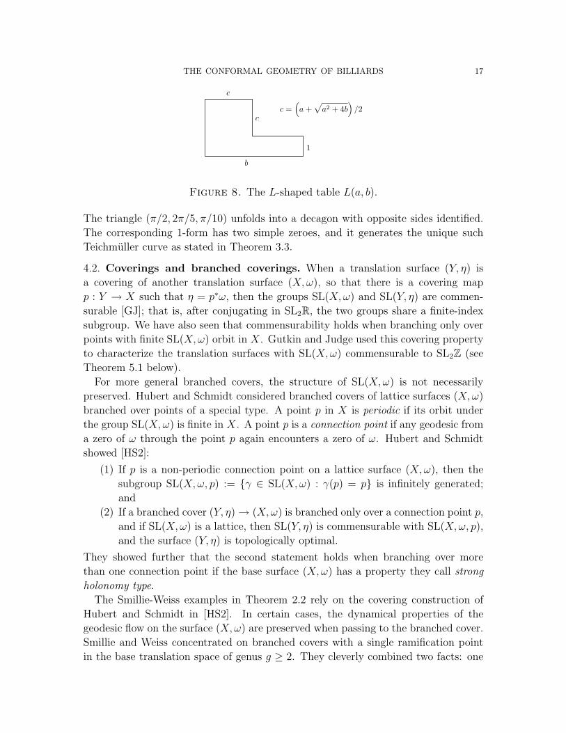
following classification of lattice polygons. For any pair of integers a and b with

b > 0, the billiard table L(a, b) is shown in Figure 8. Two tables are equivalent if

their unfolded surfaces lie in the same SL2R orbit.

Theorem 4.4. [Mc5] Let T be a billiard table which unfolds into a translation surface

(X, ω) of genus 2. Then T is is a lattice polygon if and only if it is equivalent to

(1) a table tiled by congruent triangles of angles (π/2, π/3, π/6) or (π/2, π/4, π/4);

(2) an L-shaped table L(a, b) for some a, b ∈ Z; or

(3) the triangle (π/2, 2π/5, π/10).

THE CONFORMAL GEOMETRY OF BILLIARDS 17

cc =

!a +

"a2 + 4b

#/2

1

b

c

Figure 8. The L-shaped table L(a, b).

The triangle (π/2, 2π/5, π/10) unfolds into a decagon with opposite sides identified.

The corresponding 1-form has two simple zeroes, and it generates the unique such

Teichmuller curve as stated in Theorem 3.3.

4.2. Coverings and branched coverings. When a translation surface (Y, η) is

a covering of another translation surface (X, ω), so that there is a covering map

p : Y → X such that η = p∗ω, then the groups SL(X,ω) and SL(Y, η) are commen-

surable [GJ]; that is, after conjugating in SL2R, the two groups share a finite-index

subgroup. We have also seen that commensurability holds when branching only over

points with finite SL(X, ω) orbit in X. Gutkin and Judge used this covering property

to characterize the translation surfaces with SL(X, ω) commensurable to SL2Z (see

Theorem 5.1 below).

For more general branched covers, the structure of SL(X, ω) is not necessarily

preserved. Hubert and Schmidt considered branched covers of lattice surfaces (X,ω)

branched over points of a special type. A point p in X is periodic if its orbit under

the group SL(X, ω) is finite in X. A point p is a connection point if any geodesic from

a zero of ω through the point p again encounters a zero of ω. Hubert and Schmidt

showed [HS2]:

(1) If p is a non-periodic connection point on a lattice surface (X,ω), then the

subgroup SL(X, ω, p) := γ ∈ SL(X, ω) : γ(p) = p is infinitely generated;

and

(2) If a branched cover (Y, η) → (X,ω) is branched only over a connection point p,

and if SL(X,ω) is a lattice, then SL(Y, η) is commensurable with SL(X,ω, p),

and the surface (Y, η) is topologically optimal.

They showed further that the second statement holds when branching over more

than one connection point if the base surface (X, ω) has a property they call strong

holonomy type.

The Smillie-Weiss examples in Theorem 2.2 rely on the covering construction of

Hubert and Schmidt in [HS2]. In certain cases, the dynamical properties of the

geodesic flow on the surface (X, ω) are preserved when passing to the branched cover.

Smillie and Weiss concentrated on branched covers with a single ramification point

in the base translation space of genus g ≥ 2. They cleverly combined two facts: one

18 LAURA DE MARCO

is the simple observation that the forgetful map from Mg,1 down to Mg has compact

fibers. The second is Masur’s Theorem 3.1.

4.3. The triangle of Theorem 1.3. Recall from Theorem 1.3 that the triangular

billiard table with angles (2π/5, 3π/10, 3π/10) is topologically optimal but not ergod-

ically optimal. In [CHM1], where Theorem 1.3 is proved, the authors again use one of

the Hubert-Schmidt branched covers, but branched over two points. The special ex-

ample of Theorem 1.3 arises in the following way. Begin with the translation surface

of the triangle with angles (π/2, π/5, 3π/10). This triangle unfolds into two reflected

copies of the regular pentagon, forming a surface of genus 2. It is a lattice polygon

and therefore ergodically optimal [Ve]; in fact, the triangle is equivalent to one of

the L-shaped tables in McMullen’s classification Theorem 4.4 [Mc1, §9]. The centers

of the two pentagons are connection points (see definition in §4.2). Taking a double

cover of this genus 2 surface, branched over the two centers, produces the translation

surface of genus 4 which is the unfolding of the triangle (2π/5, 3π/10, 3π/10). The

new surface is topologically optimal by the arguments of [HS2], but Cheung, Hubert,

and Masur show that it has non-uniformly distributed, dense geodesics.

4.4. Possible characterization of the lattice condition: rational ratios of

moduli. The schematic of Figure 7 indicates the relative inclusions of translation

surfaces (or billiard tables) which have lattice group SL(X, ω), those which are er-

godically optimal, and those which are topologically optimal. By McMullen’s theorem

(Corollary 4.2), the sets coincide for translation surfaces of genus 2. The examples

of Smillie and Weiss (Theorem 2.2) and of Cheung, Hubert, and Masur (Theorem

1.3) show that the containments are strict in the setting of translation surfaces of

arbitrary genus. Note, however, that Theorem 2.2 leaves open the existence of er-

godically optimal billiard tables which unfold into surfaces with non-lattice SL(X, ω),

but a search is under way.

Further investigations are also in progress about possible characterizations of the

lattice condition, because it is the geometry of the SL2R action on the moduli space of

translation surfaces which drives most of the interest in this class of billiards. In par-

ticular, there are many consequences of the lattice condition, other than ergodically

optimal geodesic flow, described in Veech’s article [Ve].

For example, suppose we fix a direction θ in which all geodesics on (X, ω) are

closed. The periodic trajectories decompose X into a finite collection of open cylin-

ders, foliated by the closed geodesics. Recall that the modulus of a Euclidean cylinder

is its height over its circumference. When SL(X, ω) forms a lattice in SL2R, the ratio

of moduli for any pair of these cylinders is rational. This is because each periodic

direction on (X, ω) corresponds to a parabolic element of SL(X, ω) which preserves

the foliation, acting by a Dehn twist on the foliated cylinders. It is possible that

THE CONFORMAL GEOMETRY OF BILLIARDS 19

SL(X, ω) is always a lattice when (X, ω) is ergodically optimal and the moduli of

cylinders in periodic directions have rational ratios.

5. Examples of groups SL(X,ω) and the search for optimal billiard

tables

In this final section, we include a collection of recent results describing groups that

arise as SL(X,ω) and some lists of billiard tables known to be lattice polygons. We

conclude with Schwartz’s recent result on periodic trajectories outside the setting of

rational polygons, as an example of the new challenges that arise in general.

5.1. Arithmetic groups. Recall from Theorem 1.1 that any billiard table which is

tiled by squares must be ergodically optimal. In fact, the unfolded surface (X, ω) is

a branched cover of a square torus, branched over a single point; consequently the

group SL(X, ω) is commensurable to the lattice SL2Z. Such subgroups of SL2R are

called arithmetic. Gutkin and Judge provided a converse to this result, characterizing

translation surfaces with arithmetic SL(X, ω).

Theorem 5.1. [GJ] The group SL(X, ω) is commensurable with SL2Z if and only if

the translation surface (X, ω) is tiled by a Euclidean parallellogram.

Recently, Ellenberg and McReynolds took this result further, by addressing which

arithmetic groups arise as the group SL(X,ω) for some translation surface.

Theorem 5.2. [EMc] Let Γ be any finite index subgroup of SL2Z which contains

±I and is contained in the level two congruence subgroup

Γ(2) =

(a b

c d

)≡(

1 0

0 1

)mod 2

.

Then there is a compact translation surface (X, ω) with SL(X, ω) isomorphic to Γ.

In their article, Ellenberg and McReynolds also show that any algebraic curve X

defined over Q is birationally equivalent to a Teichmuller curve. By Belyi’s theorem,

such an X is birationally equivalent to an unramified cover X of Σ = CP1 \0, 1,∞.Therefore, Γ = π1(X) may be viewed as a subgroup of PΓ(2) = Γ(2)/±I. The

geometric idea of their argument is to realize X as a Teichmuller curve, or, in algebro-

geometric terms, a moduli space of covers of genus-1 algebraic curves branched at 1

point.

5.2. Triangle groups. The classical triangle group, depending on integer parameters

m, n, l ≥ 2, has the finite presentation

∆(m, n, l) = 〈a, b, c | a2 = b2 = c2 = (ac)m = (bc)n = (ca)l = 1〉.

For different choices of the parameters, the group can be realized as the reflection

group in the three sides of a Euclidean, spherical, or hyperbolic triangle.

20 LAURA DE MARCO

For l = ∞, with 2 ≤ m ≤ n and mn ≥ 6, the group

∆(m, n,∞) = 〈a, b, c | a2 = b2 = c2 = (ac)m = (bc)n = 1〉

may be realized as a subgroup of PGL(2, R), by reflections in a hyperbolic triangle

with one ideal vertex, a vertex of angle π/m and a vertex of angle π/n. Restricting

to the elements that preserve orientation of the hyperbolic plane, we obtain the index

two subgroup

∆+(m, n,∞) = ∆(m, n,∞) ∩ PSL(2, R)

forming a lattice that we will call a Fuchsian triangle group. Among the Fuchsian

triangle groups, only the pairs (m, n) ∈ (2, 3), (2, 4), (2, 6), (3, 3), (4, 4), (6, 6) are

arithmetic [Ta].

The first non-arithmetic lattice groups SL(X, ω) associated to billiard tables were

provided by Veech, in his seminal 1989 article [Ve]. He showed that for each n ≥ 3,

the Fuchsian triangle group ∆+(2, n,∞) (or an index 2 subgroup, depending on the

parity of n) is the group PSL(X, ω) associated to billiards in the isosceles triangle

(π/n, π/n, (n−2)π/n). Here, PSL(X, ω) is the image of SL(X, ω) under the projection

SL2R → PSL2R = SL2R/±I. In particular, he showed that these triangular billiard

tables are ergodically optimal.

Building on Veech’s work, Ward studied billiards in the triangle (π/2n, π/n, (2n−3)π/2n). He concluded that for all n ≥ 4, this triangular table is a lattice polygon.

The associated group is PSL(X, ω) = ∆+(3, n,∞) [Wa].

By defining explicit Teichmuller curves in the moduli space, Bouw and Moller

provided the following generalization of Veech and Ward’s constructions:

Theorem 5.3. [BM2] For each pair of integers (m, n), with 1 < m < n < ∞ and

m and n not both even, there exists a translation surface (X, ω) with PSL(X, ω) =

∆+(m, n,∞).

For the case m = n, the construction of Bouw and Moller yields a translation surface

with PSL(X, ω) isomorphic to either ∆+(m, m,∞) or ∆+(2, m,∞). The ambiguity

comes from the inclusion ∆+(m, m,∞) ⊂ ∆+(2, m,∞). For the cases 2 ≤ m ≤ 5

and m < n not both even, Bouw and Moller show that their examples come from

billiard tables: they construct a triangle or quadrilateral for each such pair (m, n).

For m = 2, 3, they recover the triangles of Veech and Ward.

In [Ho2], Hooper gave an alternate construction of translation surfaces satisfy-

ing the conclusion of Theorem 5.3. He showed further that the triangle groups

∆+(m, n,∞) can not be contained in the group PSL(X,ω) of any translation sur-

face when either gcd(m, n) = 2 or both m and n are even while m/ gcd(m, n) and

n/ gcd(m, n) are both odd.

5.3. Infinitely generated groups. While the group SL(X, ω) is known to always

be discrete, it can happen that it is infinitely generated. The first such examples were

THE CONFORMAL GEOMETRY OF BILLIARDS 21

seen by Hubert and Schmidt using their branched cover construction; see §4.2. On

the other hand, McMullen showed that SL(X,ω) is often infinitely generated, at least

in genus 2. He showed that when the 1-form ω has two simple zeroes, and if SL(X,ω)

contains an element with irrational trace, then either (X, ω) lies in the SL2R orbit of

the triangle (π/2, 2π/5, π/10) or SL(X, ω) is infinitely generated.

5.4. Triangles and the continued search. While a great deal of progress has

been made towards the classification of lattice polygons, we are far from a complete

understanding, even in the restricted setting of triangles. We conclude the article

with two interesting results about these seemingly simple three-sided billiard tables.

After Veech studied the isosceles triangles mentioned in §5.2, a search began for

more examples of triangular lattice polygons. Kenyon and Smillie provided a striking

breakthrough with the following result:

Theorem 5.4. [KS] Let T be a triangle with all angles ≤ π/2. Then T is a lattice

polygon if and only if its angles are in the following list:

• (π/2, π/n, (n− 2)π/2n) for n ≥ 4

• (π/n, (n− 2)π/4n, (n− 2)π/4n) for n ≥ 3

• (π/4, π/3, 5π/12)

• (π/5, π/3, 7π/15)

• (2π/9, π/3, 4π/9)

In [KS], the theorem for acute non-isosceles triangles was stated with an extra hy-

pothesis; the proof was completed in [Pu]. It has not yet been established exactly

which acute or right triangles are ergodically optimal.

Finally, we mention that little is known once the billiard tables are allowed to

have irrational angles. Recall that all polygonal billiard tables with angles equal to

rational multiples of π have many periodic trajectories; see §2.4. By contrast, it is an

open question whether every triangular billiard table, allowing arbitrary angles, has

a periodic trajectory. In a recent article, Schwartz has shown:

Theorem 5.5. [Sch] Let T be an obtuse triangle (with rational or irrational angles)

with its largest angle no greater than 100 degrees. Then T has a stable periodic billiard

trajectory.

Stable means that all nearby triangles have a periodic trajectory of the same com-

binatorial type; see [Sch] and the references there. We may compare Theorem 5.5

to the fact that every right triangle has periodic trajectories, but Hooper has shown

that these trajectories can never be stable [Ho1].

22 LAURA DE MARCO

References

[BM1] M. Bainbridge and M. Moller. Deligne-Mumford compactification of the real multiplicationlocus and Teichmuller curves in genus three. Preprint, 2009.

[BM2] I. Bouw and M. Moller. Teichmuller curves, triangle groups, and Lyapunov exponents. Toappear, Ann. of Math. (2).

[Ca] K. Calta. Veech surfaces and complete periodicity in genus two. J. Amer. Math. Soc.17(2004), 871–908.

[Ch] Y. Cheung. Hausdorff dimension of the set of nonergodic directions. Ann. of Math. (2)158(2003), 661–678. With an appendix by M. Boshernitzan.

[CHM1] Y. Cheung, P. Hubert, and H. Masur. Topological dichotomy and strict ergodicity fortranslation surfaces. Ergodic Theory Dynam. Systems 28(2008), 1729–1748.

[CHM2] Y. Cheung, P. Hubert, and H. Masur. Dichotomy for the Hausdorff dimension of the set ofnonergodic directions. Preprint, 2009.

[CM] Y. Cheung and H. Masur. Minimal non-ergodic directions on genus-2 translation surfaces.Ergodic Theory Dynam. Systems 26(2006), 341–351.

[EMc] J. Ellenberg and D. B. McReynolds. Every curve is a Teichmuller curve. Preprint, 2009.[Gu] E. Gutkin. Billiards on almost integrable polyhedral surfaces. Ergodic Theory Dynam. Sys-

tems 4(1984), 569–584.[GJ] E. Gutkin and C. Judge. Affine mappings of translation surfaces: geometry and arithmetic.

Duke Math. J. 103(2000), 191–213.[Ho1] W. P. Hooper. Periodic billiard paths in right triangles are unstable. Geom. Dedicata

125(2007), 39–46.[Ho2] W. P. Hooper. Grid graphs and lattice surfaces. Preprint, 2009.[Hu] J. H. Hubbard. Teichmuller theory and applications to geometry, topology, and dynamics.

Vol. 1. Matrix Editions, Ithaca, NY, 2006.[HS1] P. Hubert and T. A. Schmidt. Invariants of translation surfaces. Ann. Inst. Fourier (Greno-

ble) 51(2001), 461–495.[HS2] P. Hubert and T. A. Schmidt. Infinitely generated Veech groups. Duke Math. J. 123(2004),

49–69.[KZ] A. B. Katok and A. N. Zemljakov. Topological transitivity of billiards in polygons. Mat.

Zametki 18(1975), 291–300.[KS] R. Kenyon and J. Smillie. Billiards on rational-angled triangles. Comment. Math. Helv.

75(2000), 65–108.[KMS] S. Kerckhoff, H. Masur, and J. Smillie. Ergodicity of billiard flows and quadratic differen-

tials. Ann. of Math. (2) 124(1986), 293–311.[Ma1] H. Masur. Hausdorff dimension of the set of nonergodic foliations of a quadratic differential.

Duke Math. J. 66(1992), 387–442.[Ma2] H. Masur. Ergodic theory of translation surfaces. In Handbook of dynamical systems. Vol.

1B, pages 527–547. Elsevier B. V., Amsterdam, 2006.[MT] H. Masur and S. Tabachnikov. Rational billiards and flat structures. In Handbook of dy-

namical systems, Vol. 1A, pages 1015–1089. North-Holland, Amsterdam, 2002.[Mc1] C. T. McMullen. Billiards and Teichmuller curves on Hilbert modular surfaces. J. Amer.

Math. Soc. 16(2003), 857–885.[Mc2] C. T. McMullen. Teichmuller curves in genus two: discriminant and spin. Math. Ann.

333(2005), 87–130.

THE CONFORMAL GEOMETRY OF BILLIARDS 23

[Mc3] C. T. McMullen. Teichmuller curves in genus two: the decagon and beyond. J. ReineAngew. Math. 582(2005), 173–199.

[Mc4] C. T. McMullen. Prym varieties and Teichmuller curves. Duke Math. J. 133(2006), 569–590.

[Mc5] C. T. McMullen. Teichmuller curves in genus two: torsion divisors and ratios of sines.Invent. Math. 165(2006), 651–672.

[Mc6] C. T. McMullen. Dynamics of SL2(R) over moduli space in genus two. Ann. of Math. (2)165(2007), 397–456.

[Mo1] M. Moller. Periodic points on Veech surfaces and the Mordell-Weil group over a Teichmullercurve. Invent. Math. 165(2006), 633–649.

[Mo2] M. Moller. Affine groups of flat surfaces. In Handbook of Teichmuller theory. Vol. II, vol-ume 13 of IRMA Lect. Math. Theor. Phys., pages 369–387. Eur. Math. Soc., Zurich, 2009.

[Pu] J.-C. Puchta. On triangular billiards. Comment. Math. Helv. 76(2001), 501–505.[Ra] M. Ratner. Interactions between ergodic theory, Lie groups, and number theory. In Pro-

ceedings of the International Congress of Mathematicians, Vol. 1, 2 (Zurich, 1994), pages157–182, Basel, 1995. Birkhauser.

[Sch] R. E. Schwartz. Obtuse triangular billiards. II. One hundred degrees worth of periodictrajectories. Experiment. Math. 18(2009), 137–171.

[SW] J. Smillie and B. Weiss. Veech’s dichotomy and the lattice property. Ergodic Theory Dynam.Systems 28(2008), 1959–1972.

[Ta] K. Takeuchi. Arithmetic triangle groups. J. Math. Soc. Japan 29(1977), 91–106.[Ve] W. A. Veech. Teichmuller curves in moduli space, Eisenstein series and an application to

triangular billiards. Invent. Math. 97(1989), 553–583.[Wa] C. C. Ward. Calculation of Fuchsian groups associated to billiards in a rational triangle.

Ergodic Theory Dynam. Systems 18(1998), 1019–1042.

Department of Mathematics, Statistics, and Computer Science, University of

Illinois at Chicago, demarco@math.uic.edu