Learning and stabilization of winner-take-all dynamics ... · Binas et al. Learning and stabilization of WTA dynamics a functional WTA network with structured connectivity. Due to

ORIGINAL RESEARCH ARTICLEpublished: 08 July 2014

doi: 10.3389/fncom.2014.00068

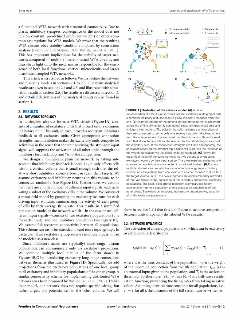
Learning and stabilization of winner-take-all dynamicsthrough interacting excitatory and inhibitory plasticityJonathan Binas1*, Ueli Rutishauser 2,3, Giacomo Indiveri1 and Michael Pfeiffer1

1 Institute of Neuroinformatics, University of Zurich and ETH Zurich, Zurich, Switzerland2 Department of Neurosurgery and Department of Neurology, Cedars-Sinai Medical Center, Los Angeles, CA, USA3 Computation and Neural Systems Program, Division of Biology and Biological Engineering, California Institute of Technology, Pasadena, CA, USA

Edited by:

Cristina Savin, IST Austria, Austria

Reviewed by:

Yanqing Chen, The NeurosciencesInstitute, USACristina Savin, IST Austria, Austria

*Correspondence:

Jonathan Binas, Institute ofNeuroinformatics, University ofZurich and ETH Zurich,Winterthurerstrasse 190,Zurich 8057, Switzerlande-mail: [email protected]

Winner-Take-All (WTA) networks are recurrently connected populations of excitatory andinhibitory neurons that represent promising candidate microcircuits for implementingcortical computation. WTAs can perform powerful computations, ranging fromsignal-restoration to state-dependent processing. However, such networks requirefine-tuned connectivity parameters to keep the network dynamics within stable operatingregimes. In this article, we show how such stability can emerge autonomously through aninteraction of biologically plausible plasticity mechanisms that operate simultaneously onall excitatory and inhibitory synapses of the network. A weight-dependent plasticity ruleis derived from the triplet spike-timing dependent plasticity model, and its stabilizationproperties in the mean-field case are analyzed using contraction theory. Our main resultprovides simple constraints on the plasticity rule parameters, rather than on the weightsthemselves, which guarantee stable WTA behavior. The plastic network we present isable to adapt to changing input conditions, and to dynamically adjust its gain, thereforeexhibiting self-stabilization mechanisms that are crucial for maintaining stable operation inlarge networks of interconnected subunits. We show how distributed neural assembliescan adjust their parameters for stable WTA function autonomously while respectinganatomical constraints on neural wiring.

Keywords: winner-take-all, competition, plasticity, self-organization, contraction theory, canonical microcircuits,

inhibitory plasticity

1. INTRODUCTIONCompetition through shared inhibition is a powerful model ofneural computation (Maass, 2000; Douglas and Martin, 2007).Competitive networks are typically composed of populations ofexcitatory neurons driving a common set of inhibitory neurons,which in turn provide global negative feedback to the excita-tory neurons (Amari and Arbib, 1977; Douglas and Martin, 1991;Hertz et al., 1991; Coultrip et al., 1992; Douglas et al., 1995;Hahnloser et al., 2000; Maass, 2000; Rabinovich et al., 2000;Yuille and Geiger, 2003; Rutishauser et al., 2011). Winner-take-all (WTA) networks are one instance of this circuit motif, whichhas been studied extensively. Neurophysiological and anatomicalstudies have shown that WTA circuits model essential featuresof cortical networks (Douglas et al., 1989; Mountcastle, 1997;Binzegger et al., 2004; Douglas and Martin, 2004; Carandiniand Heeger, 2012). An individual WTA circuit can implement avariety of non-linear operations such as signal restoration, ampli-fication, filtering, or max-like winner selection, e.g., for decisionmaking (Hahnloser et al., 1999; Maass, 2000; Yuille and Geiger,2003; Douglas and Martin, 2007). The circuit plays an essentialrole in both early and recent models of unsupervised learning,such as receptive field development (von der Malsburg, 1973;Fukushima, 1980; Ben-Yishai et al., 1995), or map formation(Willshaw and Von Der Malsburg, 1976; Amari, 1980; Kohonen,1982; Song and Abbott, 2001). Multiple WTA instances can be

combined to implement more powerful computations that can-not be achieved with a single instance, such as state dependentprocessing (Rutishauser and Douglas, 2009; Neftci et al., 2013).This modularity has given rise to the idea of WTA circuits rep-resenting canonical microcircuits, which are repeated many timesthroughout cortex and are modified slightly and combined indifferent ways to implement different functions (Douglas andMartin, 1991, 2004; Rutishauser et al., 2011).

In most models of WTA circuits the network connectivity isgiven a priori. In turn, little is known about whether and howsuch connectivity could emerge without precise pre-specification.In this article we derive analytical constraints under which localsynaptic plasticity on all connections of the network tunes theweights for WTA-type behavior. This is challenging as high-gainWTA operation on the one hand, and stable network dynamics onthe other hand, impose diverging constraints on the connectionstrengths (Rutishauser et al., 2011), which should not be violatedby the plasticity mechanism. Previous models like Jug et al. (2012)or Bauer (2013) have shown empirically that functional WTA-likebehavior can arise from an interplay of plasticity on excitatorysynapses and homeostatic mechanisms. Here, we provide a math-ematical explanation for this phenomenon, using a mean-fieldbased analysis, and derive conditions under which biologicallyplausible plasticity rules applied to all connections of a networkof randomly connected inhibitory and excitatory units produce

Frontiers in Computational Neuroscience www.frontiersin.org July 2014 | Volume 8 | Article 68 | 1

COMPUTATIONAL NEUROSCIENCE

http://www.frontiersin.org/Computational_Neuroscience/editorialboard



http://www.frontiersin.org/Computational_Neuroscience/about

http://www.frontiersin.org/Computational_Neuroscience

http://www.frontiersin.org/journal/10.3389/fncom.2014.00068/abstract

http://community.frontiersin.org/people/u/111054




mailto:[email protected]


http://www.frontiersin.org

http://www.frontiersin.org/Computational_Neuroscience/archive

Binas et al. Learning and stabilization of WTA dynamics

a functional WTA network with structured connectivity. Due toplastic inhibitory synapses, convergence of the model does notrely on constant, pre-defined inhibitory weights or other com-mon assumptions for WTA models. We prove that the resultingWTA circuits obey stability conditions imposed by contractionanalysis (Lohmiller and Slotine, 1998; Rutishauser et al., 2011).This has important implications for the stability of larger net-works composed of multiple interconnected WTA circuits, andthus sheds light onto the mechanisms responsible for the emer-gence of both local functional cortical microcircuits and largerdistributed coupled WTA networks.

This article is structured as follows: We first define the networkand plasticity models in sections 2.1 to 2.3. Our main analyticalresults are given in sections 2.4 and 2.5, and illustrated with simu-lation results in section 2.6. The results are discussed in section 3,and detailed derivations of the analytical results can be found insection 4.

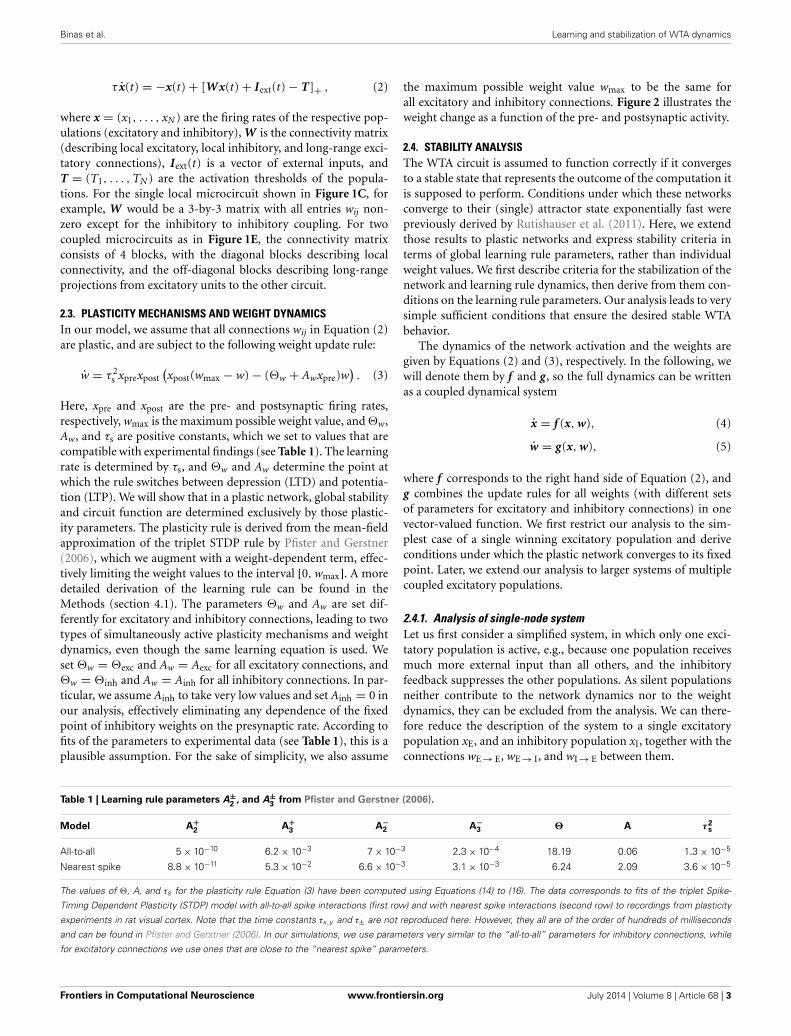
2. RESULTS2.1. NETWORK TOPOLOGYIn its simplest abstract form, a WTA circuit (Figure 1A) con-sists of a number of excitatory units that project onto a commoninhibitory unit. This unit, in turn, provides recurrent inhibitoryfeedback to all excitatory units. Given appropriate connectionstrengths, such inhibition makes the excitatory units compete foractivation in the sense that the unit receiving the strongest inputsignal will suppress the activation of all other units through theinhibitory feedback loop, and “win” the competition.

We design a biologically plausible network by taking intoaccount that inhibitory feedback is local, i.e., it only affects cellswithin a cortical volume that is small enough such that the rel-atively short inhibitory axonal arbors can reach their targets. Weassume excitatory and inhibitory neurons in this volume to beconnected randomly (see Figure 1B). Furthermore, we assumethat there are a finite number of different input signals, each acti-vating a subset of the excitatory cells in the volume. We constructa mean-field model by grouping the excitatory neurons for eachdriving input stimulus, summarizing the activity of each groupof cells by their average firing rate. This results in a simplifiedpopulation model of the network which—in the case of two dif-ferent input signals—consists of two excitatory populations (onefor each input), and one inhibitory population (see Figure 1C).We assume full recurrent connectivity between all populations.This scheme can easily be extended toward more input groups. Inparticular, if an excitatory group receives multiple inputs, it canbe modeled as a new class.

Since inhibitory axons are (typically) short-range, distantpopulations can communicate only via excitatory projections.We combine multiple local circuits of the form shown inFigures 1B,C by introducing excitatory long-range connectionsbetween them, as illustrated in Figure 1D. Specifically, we addprojections from the excitatory populations of one local groupto all excitatory and inhibitory populations of the other group. Asimilar connectivity scheme for implementing distributed WTAnetworks has been proposed by Rutishauser et al. (2012). Unliketheir model, our network does not require specific wiring, butrather targets any potential cell in the other volume. We will

FIGURE 1 | Illustration of the network model. (A) Abstractrepresentation of a WTA circuit, where several excitatory units project ontoa common inhibitory unit, and receive global inhibitory feedback from thatunit. (B) Example volume of the generic cortical structure that is assumed,consisting of (initially randomly connected) excitatory (pyramidal) cells andinhibitory interneurons. The color of the cells indicates the input channelthey are connected to: some cells only receive input from the blue, othersfrom the orange source. It is assumed that the volume is sufficiently small,such that all excitatory cells can be reached by the (short-ranged) axons ofthe inhibitory cells. If the connection strengths are tuned appropriately, thepopulation receiving the stronger input signal will suppress the response ofthe weaker population via the global inhibitory feedback. (C) shows themean field model of the same network that we construct by groupingexcitatory neurons by their input source. The three resulting excitatory andinterneuron populations are connected in an all-to-all fashion. (D,E) showmultiple, distant volumes which are connected via long-range excitatoryconnections. Projections from one volume to another connect to all cells ofthe target volume. In (E), the two subgroups are approximated by networksof the type shown in (C), consisting of one inhibitory and several excitatorypopulations. The black, solid arrows represent exemplary excitatoryconnections from one population of one group to all populations of theother group. Equivalent connections, indicated by dotted arrows, exist forall of the excitatory populations.

show in section 2.4.4 that this is sufficient to achieve competitionbetween units of spatially distributed WTA circuits.

2.2. NETWORK DYNAMICSThe activation of a neural populations xi, which can be excitatoryor inhibitory, is described by

τixi(t) = −xi(t) +⎡⎣∑

j

wijxj(t) + Iext,i(t) − Ti

⎤⎦

+, (1)

where τi is the time constant of the population, wij is the weightof the incoming connection from the jth population, Iext,i(t) isan external input given to the population, and Ti is the activationthreshold. Furthermore, [v]+ := max (0, v) is a half-wave rectifi-cation function, preventing the firing rates from taking negativevalues. Assuming identical time constants for all populations, i.e.,τi = τ for all i, the dynamics of the full system can be written as






τ x(t) = −x(t) + [Wx(t) + Iext(t) − T]+ , (2)

where x = (x1, . . . , xN ) are the firing rates of the respective pop-ulations (excitatory and inhibitory), W is the connectivity matrix(describing local excitatory, local inhibitory, and long-range exci-tatory connections), Iext(t) is a vector of external inputs, andT = (T1, . . . , TN ) are the activation thresholds of the popula-tions. For the single local microcircuit shown in Figure 1C, forexample, W would be a 3-by-3 matrix with all entries wij non-zero except for the inhibitory to inhibitory coupling. For twocoupled microcircuits as in Figure 1E, the connectivity matrixconsists of 4 blocks, with the diagonal blocks describing localconnectivity, and the off-diagonal blocks describing long-rangeprojections from excitatory units to the other circuit.

2.3. PLASTICITY MECHANISMS AND WEIGHT DYNAMICSIn our model, we assume that all connections wij in Equation (2)are plastic, and are subject to the following weight update rule:

w = τ 2s xprexpost

(xpost(wmax − w) − (�w + Awxpre)w

). (3)

Here, xpre and xpost are the pre- and postsynaptic firing rates,respectively, wmax is the maximum possible weight value, and �w,Aw, and τs are positive constants, which we set to values that arecompatible with experimental findings (see Table 1). The learningrate is determined by τs, and �w and Aw determine the point atwhich the rule switches between depression (LTD) and potentia-tion (LTP). We will show that in a plastic network, global stabilityand circuit function are determined exclusively by those plastic-ity parameters. The plasticity rule is derived from the mean-fieldapproximation of the triplet STDP rule by Pfister and Gerstner(2006), which we augment with a weight-dependent term, effec-tively limiting the weight values to the interval [0, wmax]. A moredetailed derivation of the learning rule can be found in theMethods (section 4.1). The parameters �w and Aw are set dif-ferently for excitatory and inhibitory connections, leading to twotypes of simultaneously active plasticity mechanisms and weightdynamics, even though the same learning equation is used. Weset �w = �exc and Aw = Aexc for all excitatory connections, and�w = �inh and Aw = Ainh for all inhibitory connections. In par-ticular, we assume Ainh to take very low values and set Ainh = 0 inour analysis, effectively eliminating any dependence of the fixedpoint of inhibitory weights on the presynaptic rate. According tofits of the parameters to experimental data (see Table 1), this is aplausible assumption. For the sake of simplicity, we also assume

the maximum possible weight value wmax to be the same forall excitatory and inhibitory connections. Figure 2 illustrates theweight change as a function of the pre- and postsynaptic activity.

2.4. STABILITY ANALYSISThe WTA circuit is assumed to function correctly if it convergesto a stable state that represents the outcome of the computation itis supposed to perform. Conditions under which these networksconverge to their (single) attractor state exponentially fast werepreviously derived by Rutishauser et al. (2011). Here, we extendthose results to plastic networks and express stability criteria interms of global learning rule parameters, rather than individualweight values. We first describe criteria for the stabilization of thenetwork and learning rule dynamics, then derive from them con-ditions on the learning rule parameters. Our analysis leads to verysimple sufficient conditions that ensure the desired stable WTAbehavior.

The dynamics of the network activation and the weights aregiven by Equations (2) and (3), respectively. In the following, wewill denote them by f and g, so the full dynamics can be writtenas a coupled dynamical system

x = f (x, w), (4)

w = g(x, w), (5)

where f corresponds to the right hand side of Equation (2), andg combines the update rules for all weights (with different setsof parameters for excitatory and inhibitory connections) in onevector-valued function. We first restrict our analysis to the sim-plest case of a single winning excitatory population and deriveconditions under which the plastic network converges to its fixedpoint. Later, we extend our analysis to larger systems of multiplecoupled excitatory populations.

2.4.1. Analysis of single-node systemLet us first consider a simplified system, in which only one exci-tatory population is active, e.g., because one population receivesmuch more external input than all others, and the inhibitoryfeedback suppresses the other populations. As silent populationsneither contribute to the network dynamics nor to the weightdynamics, they can be excluded from the analysis. We can there-fore reduce the description of the system to a single excitatorypopulation xE, and an inhibitory population xI, together with theconnections wE → E, wE → I, and wI → E between them.

Table 1 | Learning rule parameters A±2

, and A±3

from Pfister and Gerstner (2006).

Model A+2

A+3

A−2 A−

3 � A τ2s

All-to-all 5 × 10−10 6.2 × 10−3 7 × 10−3 2.3 × 10−4 18.19 0.06 1.3 × 10−5

Nearest spike 8.8 × 10−11 5.3 × 10−2 6.6 × 10−3 3.1 × 10−3 6.24 2.09 3.6 × 10−5

The values of �, A, and τs for the plasticity rule Equation (3) have been computed using Equations (14) to (16). The data corresponds to fits of the triplet Spike-

Timing Dependent Plasticity (STDP) model with all-to-all spike interactions (first row) and with nearest spike interactions (second row) to recordings from plasticity

experiments in rat visual cortex. Note that the time constants τx,y and τ± are not reproduced here. However, they all are of the order of hundreds of milliseconds

and can be found in Pfister and Gerstner (2006). In our simulations, we use parameters very similar to the “all-to-all” parameters for inhibitory connections, while

for excitatory connections we use ones that are close to the “nearest spike” parameters.






For a given set of (fixed) weights wc, Rutishauser et al. (2011)have shown by means of contraction theory (Lohmiller andSlotine, 1998) that the system of network activations x = f (x, wc)converges to its fixed point x∗ exponentially fast if its generalizedJacobian is negative definite. In our case, this condition reduces to

Re(

wE → E − 2 + (w2

E → E − 4 wI → E wE → I)1/2

)< 0. (6)

If condition (6) is met, the system is called contracting and isguaranteed to converge to its attractor state

x∗E = �Iext, (7)

x∗I = �wE → IIext, (8)

exponentially fast for any constant input Iext, where the contrac-tion rate is given by the left hand side of (6), divided by 2τ . Here,� = (1 − wE → E + wE → I wI → E)−1 corresponds to the networkgain. A more detailed derivation of the fixed point can be foundin section 4.2. Note that we have set the activation threshold Tequal to zero and provide external input Iext to the excitatory pop-ulation only. This simplifies the analysis but does not affect ourresults qualitatively.

2.4.2. Decoupling of network and weight dynamicsIn the following, we assume that the population dynamics iscontracting, i.e., that condition (6) is met, to show that the plas-ticity dynamics Equation (5) drives the weights w to a state thatis consistent with this condition. Essentially, our analysis has tobe self-consistent with respect to the contraction of the activa-tion dynamics. If we assume f and g to operate on very differenttimescales, we can decouple the two systems given by Equations(4) and (5). This is a valid assumption since neural (population)dynamics vary on timescales of tens or hundreds of milliseconds

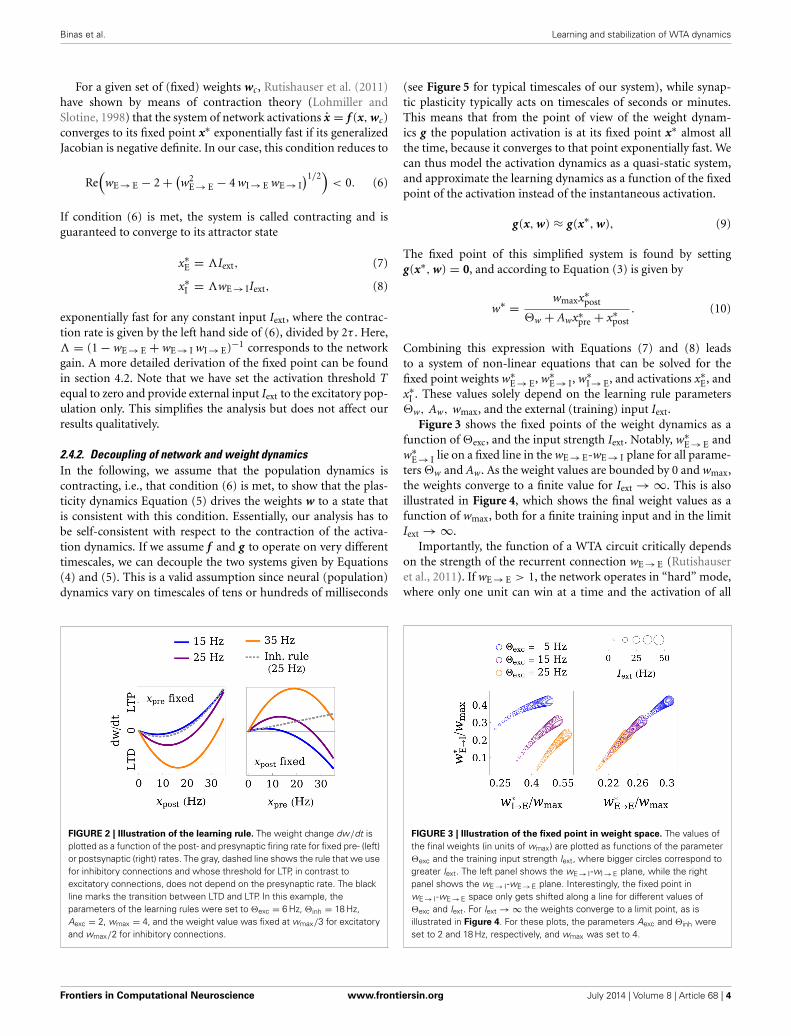
FIGURE 2 | Illustration of the learning rule. The weight change dw/dt isplotted as a function of the post- and presynaptic firing rate for fixed pre- (left)or postsynaptic (right) rates. The gray, dashed line shows the rule that we usefor inhibitory connections and whose threshold for LTP, in contrast toexcitatory connections, does not depend on the presynaptic rate. The blackline marks the transition between LTD and LTP. In this example, theparameters of the learning rules were set to �exc = 6 Hz, �inh = 18 Hz,Aexc = 2, wmax = 4, and the weight value was fixed at wmax/3 for excitatoryand wmax/2 for inhibitory connections.

(see Figure 5 for typical timescales of our system), while synap-tic plasticity typically acts on timescales of seconds or minutes.This means that from the point of view of the weight dynam-ics g the population activation is at its fixed point x∗ almost allthe time, because it converges to that point exponentially fast. Wecan thus model the activation dynamics as a quasi-static system,and approximate the learning dynamics as a function of the fixedpoint of the activation instead of the instantaneous activation.

g(x, w) ≈ g(x∗, w), (9)

The fixed point of this simplified system is found by settingg(x∗, w) = 0, and according to Equation (3) is given by

w∗ = wmaxx∗post

�w + Awx∗pre + x∗

post. (10)

Combining this expression with Equations (7) and (8) leadsto a system of non-linear equations that can be solved for thefixed point weights w∗

E → E, w∗E → I, w∗

I → E, and activations x∗E, and

x∗I . These values solely depend on the learning rule parameters

�w, Aw, wmax, and the external (training) input Iext.Figure 3 shows the fixed points of the weight dynamics as a

function of �exc, and the input strength Iext. Notably, w∗E → E and

w∗E → I lie on a fixed line in the wE → E-wE → I plane for all parame-

ters �w and Aw. As the weight values are bounded by 0 and wmax,the weights converge to a finite value for Iext → ∞. This is alsoillustrated in Figure 4, which shows the final weight values as afunction of wmax, both for a finite training input and in the limitIext → ∞.

Importantly, the function of a WTA circuit critically dependson the strength of the recurrent connection wE → E (Rutishauseret al., 2011). If wE → E > 1, the network operates in “hard” mode,where only one unit can win at a time and the activation of all

FIGURE 3 | Illustration of the fixed point in weight space. The values ofthe final weights (in units of wmax) are plotted as functions of the parameter�exc and the training input strength Iext, where bigger circles correspond togreater Iext. The left panel shows the wE → I-wI → E plane, while the rightpanel shows the wE → I-wE → E plane. Interestingly, the fixed point inwE → I-wE → E space only gets shifted along a line for different values of�exc and Iext. For Iext → ∞ the weights converge to a limit point, as isillustrated in Figure 4. For these plots, the parameters Aexc and �inh wereset to 2 and 18 Hz, respectively, and wmax was set to 4.






other units is zero. On the other hand, if wE → E is smaller than1, the network implements “soft” competition, which means thatmultiple units can be active at the same time. From Equation (27)(Methods) it follows that wE → E > 1 is possible only if wmax >

A + 1. As we will show in the following section, this conditionis necessarily satisfied by learning rules that lead to stable WTAcircuits.

2.4.3. Parameter regimes for stable network functionWe can now use the fixed points found in the previous sectionto express the condition for contraction given by condition (6) interms of the learning rule parameters. In general, this new con-dition does not assume an analytically simple form. However, wecan find simple sufficient conditions which still provide a goodapproximation to the actual value (see Methods section 4.2 fordetails). Specifically, as a key result of our analysis we derive thefollowing sufficient condition: Convergence to a point in weightspace that produces stable network dynamics is guaranteed if

Aexc + b < wmax < 2(1 + Aexc), (11)

where b is a parameter of the order 1, which is related to the mini-mum activation xE (or the minimum non-zero input Iext) duringtraining for which this condition should hold. If the minimuminput Imin that the network will be trained on is known, then b canbe computed from the fixed point x∗

E,min = x∗E (Iext = Imin), and

set to b = �exc/x∗E,min. This will guarantee contracting dynam-

ics for the full range of training inputs Iext ∈ [Imin,∞). In typicalscenarios, b can be set to a number of the order 1. This is due tothe fact that the network activation is roughly of the same orderas the input strength. Setting �exc to a value of similar order leadsto b = �exc/x∗

E,min ≈ 1.

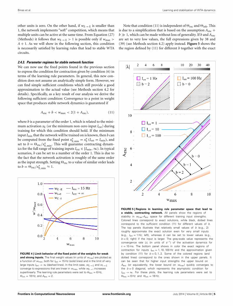
FIGURE 4 | Limit behavior of the fixed point of the weights for weak

and strong inputs. The final weight values (in units of wmax) are plotted asa function of wmax, both for Iext = 15 Hz (solid lines) and in the limit of verylarge inputs Iext → ∞ (dashed lines). In the limit case, wE → E and wI → E

converge to expressions that are linear in wmax, while wE → I increasessuperlinearly. The learning rule parameters were set to �exc = 6 Hz,�inh = 18 Hz, and Aexc = 2.

Note that condition (11) is independent of �exc and �inh. Thisis due to a simplification that is based on the assumption Aexc +b � 1, which can be made without loss of generality. If b and Aexc

are set to very low values, the full expressions given by 38 and(39) (see Methods section 4.2) apply instead. Figure 5 shows thethe region defined by (11) for different b together with the exact

FIGURE 5 | Regions in learning rule parameter space that lead to

a stable, contracting network. All panels show the regions ofstability in wmax-Aexc space for different training input strengths.Colored lines correspond to exact solutions, while black, dotted linescorrespond to the sufficient condition (11) for different values of b.The top panels illustrate that relatively small values of b (e.g., 2)roughly approximate the exact solution even for very small inputs(e.g., Iext = 1 Hz; left), whereas b can be set to lower values (e.g.,b = 0; right) if the input is larger. The gray-scale value represents theconvergence rate |λ| (in units of s−1) of the activation dynamics forτ = 10 ms. The bottom panel shows in color the exact regions ofcontraction for inputs Iext = 1, 10, 100 Hz and the approximation givenby condition (11) for b = 0, 1, 2. Some of the colored regions (anddotted lines) correspond to the ones shown in the upper panels. Itcan be seen that for higher input strengths the upper bound onAexc (or equivalently, the lower bound on wmax) quickly converges tothe b = 0 diagonal, which represents the asymptotic condition forIexc → ∞. For these plots, the learning rule parameters were set to�exc = 6 Hz and �inh = 18 Hz.






condition for contraction, indicating that (11) is indeed sufficientand that b can safely be set to a value around 1 in most cases.

2.4.4. Extension to multiple unitsSo far, we have only studied a small network that can be regardedas a single subunit of a larger, distributed WTA system. However,our results can be generalized to larger systems without mucheffort. In our model, as illustrated in Figures 1D,E, different local-ized WTA circuits can be coupled via excitatory projections. Theseprojections include excitatory-to-inhibitory connections, as wellas reciprocal connections between distant excitatory units. Inorder to demonstrate the effects of this coupling, we considertwo localized subsystems, x = (xE, xI) and x′ = (x′

E, x′I), consist-

ing of one excitatory and one inhibitory unit each. Furthermore,we add projections from xE to x′

E and x′I, as required by our

model. We denote by wE → E′ the strength of the long-rangeexcitatory-to-excitatory connection, while we refer to the long-range excitatory-to-inhibitory connection as wE → I′ . Note thatfor the sake of clarity we only consider the unidirectional casex → x′ here, while the symmetric case x ↔ x′ can be dealt withanalogously.

We first look at the excitatory-to-inhibitory connections. Ifonly xE is active and x′

E is silent, then xI and x′I are driven by

the same presynaptic population (xE), and wE → I′ converges tothe same value as wE → I. Thus, after convergence, both inhibitoryunits are perfectly synchronized in their activation when xE isactive, and an equal amount of inhibition can be provided to xE

and x′E.

Besides synchronization of inhibition, proper WTA function-ality also requires the recurrent excitation wE → E′ (between theexcitatory populations of the different subunits) to convergeto sufficiently low values, such that different units competevia the synchronized inhibition rather than exciting each otherthrough the excitatory links. As pointed out by Rutishauser et al.(2012), the network is stable and functions correctly if the recur-rent excitation between populations is lower than the recurrentself-excitation, i.e., wE → E′ < wE′ → E′ .

We now consider the case where xE and x′E receive an exter-

nal input Iext. Whenever x′E alone receives the input, there is

no interaction between the two subunits, and the recurrent self-connection wE′ → E′ converges to the value that was found forthe simplified case of a single subunit (section 2.4.2). The sameis true for the connection wE → E if xE alone receives the input.However, in this case xE and x′

E might also interact via the con-nection wE → E′ , which would then be subject to plasticity. As xprojects to x′, but not vice versa, we require xE > x′

E if both xE

and x′E receive the same input Iext, because xE should suppress x′

Evia the long-range competition mechanism. In terms of connec-tion strengths, this means that w∗

E → I′ w∗I′ → E′ > w∗

E → E′ , i.e., theinhibitory input to x′

E that is due to xE must be greater than theexcitatory input x′

E receives from xE. In the Methods (section 4.3),we show that a sufficient condition for this to be the case is

wmax > A + b + 1, (12)

which alters our results from section 2.4.3 only slightly, effec-tively shifting the lower bound on wmax by an offset of 1, as can

be seen by comparing conditions (11) and (12). On the otherhand, making use of the fact that x′

E < xE, it can be shown thatwE → E′ converges to a value smaller than wE′ → E′ (see Methodssection 4.3), as required by the stability condition mentionedabove.

2.5. GAIN CONTROL AND NORMALIZATIONIn the previous section, we showed how synaptic plasticity canbe used to drive the connection strengths toward regimes whichguarantee stable network dynamics. Since the actual fixed pointvalues of the weights change with the training input, this mech-anism can as well be used to tune certain functional propertiesof the network. Here we focus on controlling the gain of the net-work, i.e., the relationship between the strength of the strongestinput and the activation of the winning excitatory units withinthe recurrent circuit, as a function of the training input.

In the case of a single active population, the gain is given by� = xE/Iext = (1 − w∗

E → E + w∗E → I w∗

I → E)−1, as can be inferredfrom Equation (7). Depending on the gain, the network can eitheramplify (� > 1) or weaken (� < 1) the input signal.

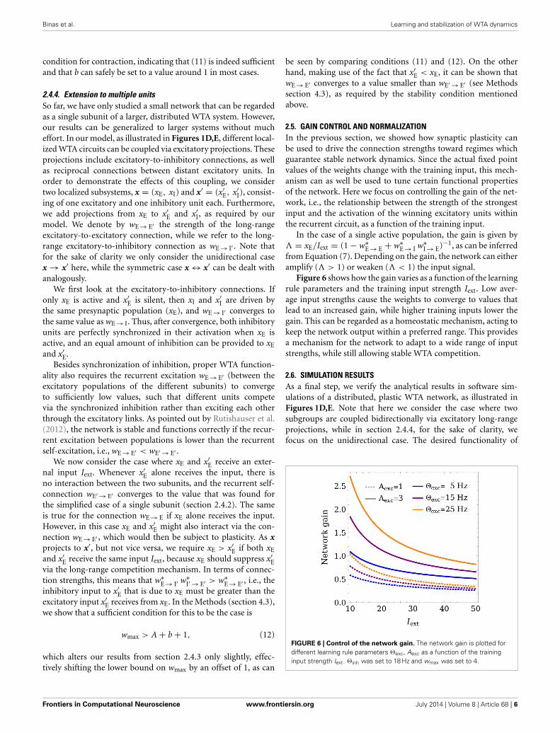
Figure 6 shows how the gain varies as a function of the learningrule parameters and the training input strength Iext. Low aver-age input strengths cause the weights to converge to values thatlead to an increased gain, while higher training inputs lower thegain. This can be regarded as a homeostatic mechanism, acting tokeep the network output within a preferred range. This providesa mechanism for the network to adapt to a wide range of inputstrengths, while still allowing stable WTA competition.

2.6. SIMULATION RESULTSAs a final step, we verify the analytical results in software sim-ulations of a distributed, plastic WTA network, as illustrated inFigures 1D,E. Note that here we consider the case where twosubgroups are coupled bidirectionally via excitatory long-rangeprojections, while in section 2.4.4, for the sake of clarity, wefocus on the unidirectional case. The desired functionality of

FIGURE 6 | Control of the network gain. The network gain is plotted fordifferent learning rule parameters �exc, Aexc as a function of the traininginput strength Iext. �inh was set to 18 Hz and wmax was set to 4.






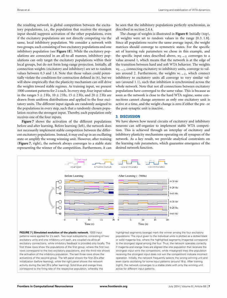
the resulting network is global competition between the excita-tory populations, i.e., the population that receives the strongestinput should suppress activation of the other populations, evenif the excitatory populations are not directly competing via thesame, local inhibitory population. We consider a network withtwo groups, each consisting of two excitatory populations and oneinhibitory population (see Figure 1E). While the excitatory pop-ulations are connected in an all-to-all manner, inhibitory pop-ulations can only target the excitatory populations within theirlocal groups, but do not form long-range projection. Initially, allconnection weights (excitatory and inhibitory) are set to randomvalues between 0.3 and 1.8. Note that those values could poten-tially violate the conditions for contraction defined in (6), but wewill show empirically that the plasticity mechanism can still drivethe weights toward stable regimes. As training input, we present1000 constant patterns for 2 s each. In every step, four input valuesin the ranges 5 ± 2 Hz, 10 ± 2 Hz, 15 ± 2 Hz, and 20 ± 2 Hz aredrawn from uniform distributions and applied to the four exci-tatory units. The different input signals are randomly assigned tothe populations in every step, such that a randomly chosen popu-lation receives the strongest input. Thereby, each population onlyreceives one of the four inputs.

Figure 7 shows the activation of the different populationsbefore and after learning. Before learning (left), the network doesnot necessarily implement stable competition between the differ-ent excitatory populations. Instead, it may end up in an oscillatingstate or amplify the wrong winning unit. However, after training(Figure 7, right), the network always converges to a stable staterepresenting the winner of the competition. Furthermore, it can

be seen that the inhibitory populations perfectly synchronize, asdescribed in section 2.4.4.

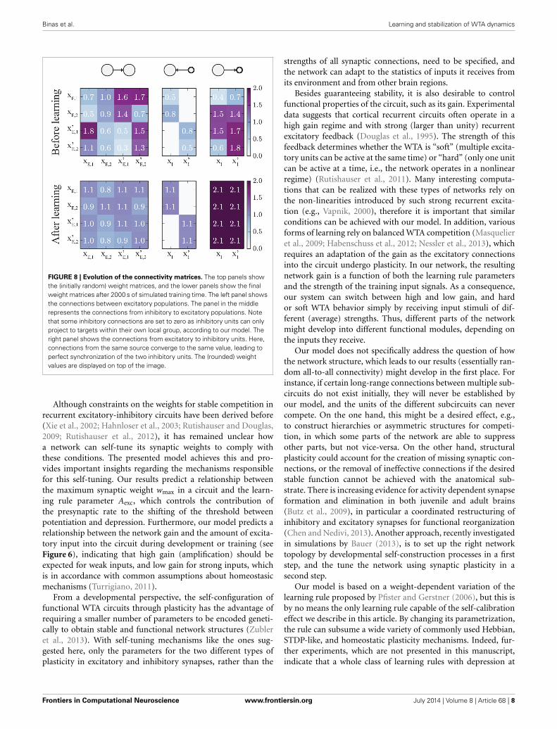
The change of weights is illustrated in Figure 8: Initially (top),all weights were set to random values in the range [0.3, 1.8].Since all populations receive the same average input, the weightmatrices should converge to symmetric states. For the specificset of learning rule parameters we chose in this example, andthe specific input rates described above, wE → E converges to avalue around 1, which means that the network is at the edge ofthe transition between hard and soft WTA behavior. The weightswE → I, connecting excitatory to inhibitory units, converge to val-ues around 2. Furthermore, the weights wI → E, which connectinhibitory to excitatory units all converge to very similar val-ues (around 1.1), such that inhibition is synchronized across thewhole network. Note that not all connections between excitatorypopulations have converged to the same value. This is because assoon as the network is close to the hard WTA regime, some con-nections cannot change anymore as only one excitatory unit isactive at a time, and the weight change is zero if either the pre- orthe post-synaptic unit is inactive.

3. DISCUSSIONWe have shown how neural circuits of excitatory and inhibitoryneurons can self-organize to implement stable WTA competi-tion. This is achieved through an interplay of excitatory andinhibitory plasticity mechanisms operating on all synapses of thenetwork. As a key result, we provide analytical constraints onthe learning rule parameters, which guarantee emergence of thedesired network function.

FIGURE 7 | Simulated evolution of the plastic network. 1000 inputpatterns were applied for 2 s each. Two local subsystems, consisting of twoexcitatory units and one inhibitory unit each, are coupled via all-to-allexcitatory connections, while inhibitory feedback is provided only locally. Thefirst three rows show the populations of the first group, where the first tworows correspond to the two excitatory populations, and the third row showsthe activation of the inhibitory population. The last three rows show theactivations of the second group. The left panel shows the first 20 s afterinitialization (before learning), while the right panel shows the networkactivity during the last 20 s (after learning). Solid blue and orange linescorrespond to the firing rate of the respective population, whereby the

highlighted segments (orange) mark the winner among the four excitatorypopulations. The input given to the individual units is plotted as a dotted blackor solid magenta line, where the highlighted segments (magenta) correspondto the strongest signal among the four. Thus, the network operates correctlyif magenta and orange lines are aligned (the one population that receives thestrongest input wins the competition), while misaligned lines (the populationreceiving the strongest input does not win the competition) indicate incorrectoperation. Initially, the network frequently selects the wrong winning unit andeven starts oscillating for some input patterns (around 18 s). After training(right), the network converges to a stable state with only the winning unitactive for different input patterns.






FIGURE 8 | Evolution of the connectivity matrices. The top panels showthe (initially random) weight matrices, and the lower panels show the finalweight matrices after 2000 s of simulated training time. The left panel showsthe connections between excitatory populations. The panel in the middlerepresents the connections from inhibitory to excitatory populations. Notethat some inhibitory connections are set to zero as inhibitory units can onlyproject to targets within their own local group, according to our model. Theright panel shows the connections from excitatory to inhibitory units. Here,connections from the same source converge to the same value, leading toperfect synchronization of the two inhibitory units. The (rounded) weightvalues are displayed on top of the image.

Although constraints on the weights for stable competition inrecurrent excitatory-inhibitory circuits have been derived before(Xie et al., 2002; Hahnloser et al., 2003; Rutishauser and Douglas,2009; Rutishauser et al., 2012), it has remained unclear howa network can self-tune its synaptic weights to comply withthese conditions. The presented model achieves this and pro-vides important insights regarding the mechanisms responsiblefor this self-tuning. Our results predict a relationship betweenthe maximum synaptic weight wmax in a circuit and the learn-ing rule parameter Aexc, which controls the contribution ofthe presynaptic rate to the shifting of the threshold betweenpotentiation and depression. Furthermore, our model predicts arelationship between the network gain and the amount of excita-tory input into the circuit during development or training (seeFigure 6), indicating that high gain (amplification) should beexpected for weak inputs, and low gain for strong inputs, whichis in accordance with common assumptions about homeostasicmechanisms (Turrigiano, 2011).

From a developmental perspective, the self-configuration offunctional WTA circuits through plasticity has the advantage ofrequiring a smaller number of parameters to be encoded geneti-cally to obtain stable and functional network structures (Zubleret al., 2013). With self-tuning mechanisms like the ones sug-gested here, only the parameters for the two different types ofplasticity in excitatory and inhibitory synapses, rather than the

strengths of all synaptic connections, need to be specified, andthe network can adapt to the statistics of inputs it receives fromits environment and from other brain regions.

Besides guaranteeing stability, it is also desirable to controlfunctional properties of the circuit, such as its gain. Experimentaldata suggests that cortical recurrent circuits often operate in ahigh gain regime and with strong (larger than unity) recurrentexcitatory feedback (Douglas et al., 1995). The strength of thisfeedback determines whether the WTA is “soft” (multiple excita-tory units can be active at the same time) or “hard” (only one unitcan be active at a time, i.e., the network operates in a nonlinearregime) (Rutishauser et al., 2011). Many interesting computa-tions that can be realized with these types of networks rely onthe non-linearities introduced by such strong recurrent excita-tion (e.g., Vapnik, 2000), therefore it is important that similarconditions can be achieved with our model. In addition, variousforms of learning rely on balanced WTA competition (Masquelieret al., 2009; Habenschuss et al., 2012; Nessler et al., 2013), whichrequires an adaptation of the gain as the excitatory connectionsinto the circuit undergo plasticity. In our network, the resultingnetwork gain is a function of both the learning rule parametersand the strength of the training input signals. As a consequence,our system can switch between high and low gain, and hardor soft WTA behavior simply by receiving input stimuli of dif-ferent (average) strengths. Thus, different parts of the networkmight develop into different functional modules, depending onthe inputs they receive.

Our model does not specifically address the question of howthe network structure, which leads to our results (essentially ran-dom all-to-all connectivity) might develop in the first place. Forinstance, if certain long-range connections between multiple sub-circuits do not exist initially, they will never be established byour model, and the units of the different subcircuits can nevercompete. On the one hand, this might be a desired effect, e.g.,to construct hierarchies or asymmetric structures for competi-tion, in which some parts of the network are able to suppressother parts, but not vice-versa. On the other hand, structuralplasticity could account for the creation of missing synaptic con-nections, or the removal of ineffective connections if the desiredstable function cannot be achieved with the anatomical sub-strate. There is increasing evidence for activity dependent synapseformation and elimination in both juvenile and adult brains(Butz et al., 2009), in particular a coordinated restructuring ofinhibitory and excitatory synapses for functional reorganization(Chen and Nedivi, 2013). Another approach, recently investigatedin simulations by Bauer (2013), is to set up the right networktopology by developmental self-construction processes in a firststep, and the tune the network using synaptic plasticity in asecond step.

Our model is based on a weight-dependent variation of thelearning rule proposed by Pfister and Gerstner (2006), but this isby no means the only learning rule capable of the self-calibrationeffect we describe in this article. By changing its parametrization,the rule can subsume a wide variety of commonly used Hebbian,STDP-like, and homeostatic plasticity mechanisms. Indeed, fur-ther experiments, which are not presented in this manuscript,indicate that a whole class of learning rules with depression at






low and potentiation at high postsynaptic firing rates would leadto similar results. We chose the triplet rule to demonstrate ourfindings as its parameters have been mapped to experiments,and also because it can be written in an analytically tractableform. We have assumed here a specific type of inhibitory plas-ticity, which analytically is of the same form as the simultane-ous excitatory plasticity, but uses different parameters. With theparameters we chose for the inhibitory plasticity rule, we obtaina form that is very similar to the one proposed by Vogels et al.(2011). By introducing inhibitory plasticity it is no longer neces-sary to make common but biologically unrealistic assumptions,like pre-specified constant and uniform inhibitory connectionstrengths (Oster et al., 2009), or more abstract forms of sum-ming up the excitatory activity in the circuit (Jug et al., 2012;Nessler et al., 2013), because inhibitory weights will automat-ically converge toward stable regions. Inhibitory plasticity hasreceived more attention recently with the introduction of newmeasurement techniques, and has revealed a great diversity ofplasticity mechanisms, in line with the diversity of inhibitorycell types (Kullmann and Lamsa, 2011; Kullmann et al., 2012).Our model involves only a single inhibitory population per localsub-circuit, which interacts with all local excitatory units. Notonly is this a common assumption in most previous models,and greatly simplifies the analysis, but also is in accordance withanatomical and electrophysiological results of relatively unspe-cific inhibitory activity in sensory cortical areas (Kerlin et al.,2010; Bock et al., 2011). However, recent studies have shown morecomplex interactions of different inhibitory cell types (Pfefferet al., 2013), making models based on diverse cell types withdifferent properties an intriguing target for future studies. Theassumption of a common inhibitory pool that connects to all exci-tatory units is justified for local circuits, but violates anatomicalconstraints on the length of inhibitory axons if interacting pop-ulations are far apart (Binzegger et al., 2005). Our results easilygeneralize to the case of distributed inhibition, by adapting themodel of Rutishauser et al. (2012) (see Figure 1E). Our contri-bution is to provide the first learning theory for these types ofcircuits.

Since our model is purely rate-based, a logical next step isto investigate how it translates into the spiking neural networkdomain. Establishing similar constraints on spike-based learn-ing rules that enable stable WTA competition remains an openproblem for future research, although Chen et al. (2013) haveshown empirically that WTA behavior in a circuit with topo-logically ordered input is possible under certain restrictions oninitial synapse strengths, and in the presence of STDP and short-term plasticity. Spiking WTA circuits can potentially utilize thericher temporal dynamics of spike trains in the sense that theorder of spikes and spike-spike correlations have an effect on theconnectivity.

Potential practical applications of our model, and futurespiking extensions, lie in neuromorphic VLSI circuits, whichhave to deal with the problem of device mismatch (Indiveriet al., 2011), and can thus not be precisely configured a pri-ori. Our model could provide a means for the circuits toself-tune and autonomously adapt to the peculiarities of thehardware.

4. MATERIALS AND METHODS4.1. DERIVATION OF THE PLASTICITY MECHANISMThe learning rule given by Equation (3) is based on the tripletSTDP rule by Pfister and Gerstner (2006). Since we are interestedin the rate dynamics, we use the mean-field approximation of thisrule, which is provided by the authors and leads to an expectedweight change of

w = xprexpost(A+

2 τ+ − A−2 τ− + A+

3 τ+τyxpost

− A−3 τ−τxxpre

), (13)

where xpre, xpost are the pre- and postsynaptic activations andA±

2 , A±3 , τ±, τx,y are parameters that determine the amplitude of

weight changes in the triplet STDP model. All of the parametersare assumed to be positive. Through a substitution of constantsgiven by

τ 2s := A+

3 τ+τy, (14)

�w := (A−

2 τ− − A+2 τ+

)/τ 2

s , (15)

Aw := A−3 τ−τx/τ

2s , (16)

the rule in Equation (13) can be written in the simpler form

w = τ 2s xprexpost

(xpost − (�w + Awxpre)

), (17)

where �w is in units of a firing rate and Aw is a unitless constant.The terms in parentheses on the right of Equation (17) can bedivided into a positive (LTP) part that depends on xpost, and anegative (LTD) part that depends on xpre. In order to constrainthe range of weights, we add weight-dependent terms m+(w) andm−(w) to the two parts of the rule, which yields

w = τ 2s xprexpost

(xpostm+(w) − (�w + Awxpre)m−(w)

). (18)

Throughout this manuscript, we use a simple, linear weightdependence m+ = wmax − w and m− = w, which effectively lim-its the possible values of weights to the interval [0, wmax]. Wechose this form, which is described by a single parameter, forreasons of analytical tractability and because it is consistent withexperimental findings (Gütig et al., 2003). In Pfister and Gerstner(2006), values for the parameters τx,y, τ±, and A±

2,3 of the ruleEquation (13) were determined from fits to experimental mea-surements in pyramidal cells in visual cortex (see Table 1) andhippocampal cultures (Bi and Poo, 1998, 2001; Sjöström et al.,2001; Wang et al., 2005). We used these values to calculate plau-sible values for �w, Aw, and τs using Equations (14) to (16). Inour simulations, we use parameters very similar to the exper-imentally derived values in Table 1. Specifically, for inhibitoryconnections we use parameters very similar to the ones foundfrom fits of experimental data to the triplet STDP model withall-to-all spike interactions. On the other hand, we choose param-eters for the excitatory plasticity rules which are close to fits of thetriplet STDP rule with nearest-neighbor spike interactions. Theparameters that were used in software simulations and to obtainmost of the numeric results are listed in Table 2. Note that for the






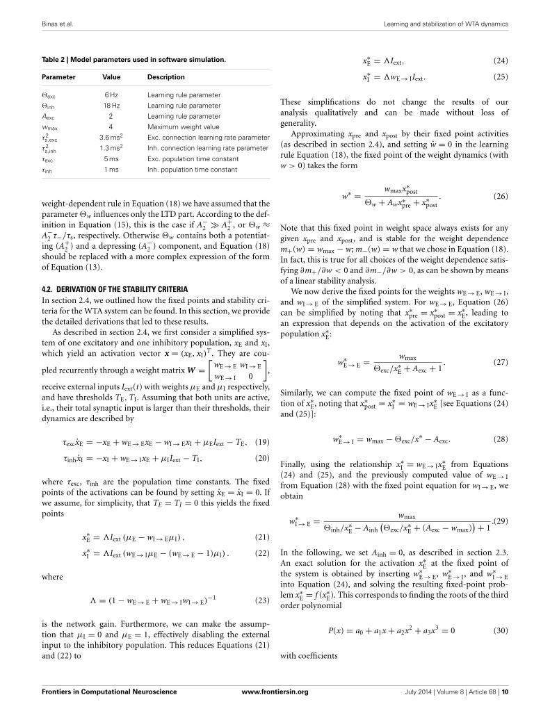
Table 2 | Model parameters used in software simulation.

Parameter Value Description

�exc 6 Hz Learning rule parameter

�inh 18 Hz Learning rule parameter

Aexc 2 Learning rule parameter

wmax 4 Maximum weight value

τ2s,exc 3.6 ms2 Exc. connection learning rate parameter

τ2s,inh 1.3 ms2 Inh. connection learning rate parameter

τexc 5 ms Exc. population time constant

τinh 1 ms Inh. population time constant

weight-dependent rule in Equation (18) we have assumed that theparameter �w influences only the LTD part. According to the def-inition in Equation (15), this is the case if A−

2 � A+2 , or �w ≈

A−2 τ−/τs, respectively. Otherwise �w contains both a potentiat-

ing (A+2 ) and a depressing (A−

2 ) component, and Equation (18)should be replaced with a more complex expression of the formof Equation (13).

4.2. DERIVATION OF THE STABILITY CRITERIAIn section 2.4, we outlined how the fixed points and stability cri-teria for the WTA system can be found. In this section, we providethe detailed derivations that led to these results.

As described in section 2.4, we first consider a simplified sys-tem of one excitatory and one inhibitory population, xE and xI,which yield an activation vector x = (xE, xI)

T . They are cou-

pled recurrently through a weight matrix W =[

wE → E wI → E

wE → I 0

],

receive external inputs Iext(t) with weights μE and μI respectively,and have thresholds TE, TI. Assuming that both units are active,i.e., their total synaptic input is larger than their thresholds, theirdynamics are described by

τexcxE = −xE + wE → ExE − wI → ExI + μEIext − TE, (19)

τinhxI = −xI + wE → IxE + μIIext − TI, (20)

where τexc, τinh are the population time constants. The fixedpoints of the activations can be found by setting xE = xI = 0. Ifwe assume, for simplicity, that TE = TI = 0 this yields the fixedpoints

x∗E = �Iext (μE − wI → EμI) , (21)

x∗I = �Iext (wE → IμE − (wE → E − 1)μI) . (22)

where

� = (1 − wE → E + wE → IwI → E)−1 (23)

is the network gain. Furthermore, we can make the assump-tion that μI = 0 and μE = 1, effectively disabling the externalinput to the inhibitory population. This reduces Equations (21)and (22) to

x∗E = �Iext, (24)

x∗I = �wE → IIext. (25)

These simplifications do not change the results of ouranalysis qualitatively and can be made without loss ofgenerality.

Approximating xpre and xpost by their fixed point activities(as described in section 2.4), and setting w = 0 in the learningrule Equation (18), the fixed point of the weight dynamics (withw > 0) takes the form

w∗ = wmaxx∗post

�w + Awx∗pre + x∗

post. (26)

Note that this fixed point in weight space always exists for anygiven xpre and xpost, and is stable for the weight dependencem+(w) = wmax − w; m−(w) = w that we chose in Equation (18).In fact, this is true for all choices of the weight dependence satis-fying ∂m+/∂w < 0 and ∂m−/∂w > 0, as can be shown by meansof a linear stability analysis.

We now derive the fixed points for the weights wE → E, wE → I,and wI → E of the simplified system. For wE → E, Equation (26)can be simplified by noting that x∗

pre = x∗post = x∗

E, leading toan expression that depends on the activation of the excitatorypopulation x∗

E:

w∗E → E = wmax

�exc/x∗E + Aexc + 1

. (27)

Similarly, we can compute the fixed point of wE → I as a func-tion of x∗

E, noting that x∗post = x∗

I = wE → Ix∗E [see Equations (24)

and (25)]:

w∗E → I = wmax − �exc/x∗ − Aexc. (28)

Finally, using the relationship x∗I = wE → Ix∗

E from Equations(24) and (25), and the previously computed value of wE → I

from Equation (28) with the fixed point equation for wI → E, weobtain

w∗I → E = wmax

�inh/x∗E − Ainh

(�exc/x∗

E + (Aexc − wmax)) + 1

.(29)

In the following, we set Ainh = 0, as described in section 2.3.An exact solution for the activation x∗

E at the fixed point ofthe system is obtained by inserting w∗

E → E, w∗E → I, and w∗

I → Einto Equation (24), and solving the resulting fixed-point prob-lem x∗

E = f (x∗E). This corresponds to finding the roots of the third

order polynomial

P(x) = a0 + a1x + a2x2 + a3x3 = 0 (30)

with coefficients






a0 = �exc�inhIext, (31)

a1 = −�exc�inh + �excIext + �inhIext + �inhAexcIext

+�2excwmax, (32)

a2 = −�exc − �inh − �inhAexc + Iext + AexcIext + �excwmax

+�inhwmax + 2�excAexcwmax − �excw2max, (33)

a3 = −1 − Aexc + wmax + Aexcwmax + A2excwmax − w2

max

− Aexcw2max. (34)

The activation of the excitatory population xE at the fixed point isthen given by the positive, real root of Equation (30).

The fixed point of the activation x∗E, and thus the fixed points

of the weights, are monotonic functions of the training inputstrength Iext (see Figure 3, for example). In the following, weinvestigate the behavior of the fixed point weight values for verylarge and very small external inputs during training, respectively.This helps us to find conditions on the learning rule param-eters that lead to stable dynamics (of the network activation)for any training input strength. We define a positive constantb := �exc/x∗

E, and plug it into Equations (27)–(29). This yields

w∗E → E = wmax

Aexc + b + 1, (35)

w∗E → I = wmax − Aexc − b, (36)

w∗I → E = wmax�exc

b �inh + �exc. (37)

Inserting Equations (35)–(37) into the condition for contrac-tion of the activation dynamics given by (6), we can describe thecondition in terms of the learning rule parameters, and a newconstant � := �exc/(�exc + b �inh):

1

(1 + Aexc + b)< � < 1, (38)

(Aexc + b)

(1 + 1

�(1 + Aexc + b)2 − 1

)< wmax

< 2(1 + Aexc + b),(39)

Assuming Aexc + b � 1 (note that we can always set Aexc to asufficiently large value), the conditions reduce to

0 < � < 1, (40)

Aexc + b < wmax < 2(1 + Aexc + b), (41)

whereby the first condition can be dropped, since � ∈ [0, 1]always holds. The second condition still depends on b, and there-fore on x∗

E. We will illustrate how to eliminate this dependenceunder very weak assumptions. First, in the limit of very largeinputs x∗

E also takes very large values, leading to b → 0 for Iext →∞. In that case, condition (41) becomes independent of b and canbe written as

Aexc < wmax < 2(1 + Aexc). (42)

On the other hand, in the case of very small inputs we have toinclude the effects of b, as b can in principle take very large values.In typical scenarios the output of the network can be assumedto be roughly of the order of its input. If �exc is chosen to be ofthe same order, then b ≈ 1. For any finite b, we can express thestability condition that is valid for all inputs as the intersection ofthe conditions for large inputs, condition (42), with the one forarbitrarily small inputs, condition (41), leading to

Aexc + b < wmax < 2(1 + Aexc). (43)

Note that this condition can be met for any finite b by choos-ing sufficiently large Aexc and wmax. However, as discussed above,choices of the parameter b of the order 1 should be sufficient fortypical scenarios, whereas higher values would guarantee stabledynamics for very low input strengths (e.g., Iext �exc). This isillustrated in Figure 5, where the exact regions of stability as afunction of wmax and Aexc are shown for different training inputstrengths, together with the sufficient conditions given by (43).In practice, a good starting point for picking a value b for whichthe stability conditions should hold is to determine the minimumnon-zero input Imin encountered during training for which thiscondition should hold, and setting b = �exc/x∗

E,min, where x∗E,min

is the fixed point activation for Iext = Imin.

4.3. EXTENSION TO MULTIPLE UNITSIn this section, we illustrate how multiple subunits, as analyzed inthe previous section, can be combined to larger WTA networkswith distributed inhibition. For the sake of simplicity, we onlyconsider the unidirectional case, where a subunit x = (xE, xI)projects onto another subunit x′ = (x′

E, x′I) via excitatory con-

nections wE → E′ and wE → I′ . The bidirectional case x ↔ x′ canbe analyzed analogously. If xE and x′

E receive the same input, theresponse of x′

E should be weaker, such that activation of xE causessuppression of x′

E rather than excitation. This means that

w∗E → E′ < w∗

E → I′ w∗I′ → E′ (44)

must hold. We assume that both subsystems have been trained oninputs of the same average strength, such that their local connec-tions have converged to the same weights, i.e., w∗

E′ → I′ = w∗E → I

and w∗I′ → E′ = w∗

I → E. Furthermore, we assume that condition(44) is true initially. This can be guaranteed by setting the ini-tial value of wE → E′ to a sufficiently small number. Our task thenis to show that condition (44) remains true for all time. Thevalues of w∗

E′ → I′ and w∗I′ → E′ , or w∗

E → I and w∗I → E respectively,

are described by Equations (36) and (37). On the other hand,according to Equation (26), the value of w∗

E → E′ is given by

w∗E → E′ = wmaxx′∗

E

�exc + Aexcx∗E + x′∗

E

. (45)

Plugging all this into condition (44) and simplifying the expres-sion, leads to the condition

wmax > Aexc + b + x′E

AexcxE + x′E + �

, (46)






which can be replaced by the sufficient condition

wmax > Aexc + b + 1, (47)

that guarantees x∗E′ < x∗

E if both excitatory populations receivethe same input. On the other hand, this result impliesw∗

E → E′ < w∗E′ → E′ , which is required for stable network dynamics

(Rutishauser et al., 2012), and can be verified by comparing therespective fixed point equations

w∗E → E′ = x′

E/(�exc + AexcxE + x′

E

), (48)

w∗E′ → E′ = x′

E/(�exc + Aexcx′

E + x′E

). (49)

4.4. SOFTWARE SIMULATIONSoftware simulations of our model were implemented using cus-tom Python code based on the “NumPy” and “Dana” packages,and run on a Linux workstation. Numerical integration of thesystem dynamics was carried out using the forward Euler methodwith a 1 ms timestep.

AUTHOR CONTRIBUTIONSJonathan Binas, Ueli Rutishauser, Giacomo Indiveri, MichaelPfeiffer conceived and designed the experiments. Jonathan Binasperformed the experiments and analysis. Jonathan Binas, UeliRutishauser, Giacomo Indiveri, Michael Pfeiffer wrote the paper.

FUNDINGThe research was supported by the Swiss National ScienceFoundation Grant 200021_146608, and the European Union ERCGrant “neuroP” (257219).

ACKNOWLEDGMENTWe thank Rodney Douglas, Peter Diehl, Roman Bauer, andour colleagues at the Institute of Neuroinformatics for fruitfuldiscussion.

REFERENCESAmari, S., and Arbib, M. (1977). “Competition and cooperation in neural nets,” in

Systems Neuroscience, ed J. Metzler (San Diego, CA: Academic Press), 119–165.Amari, S.-I. (1980). Topographic organization of nerve fields. Bull. Math. Biol. 42,

339–364. doi: 10.1007/BF02460791Bauer, R. (2013). Self-Construction and -Configuration of Functional Neuronal

Networks. PhD Thesis, ETH Zürich.Ben-Yishai, R., Bar-Or, R. L., and Sompolinsky, H. (1995). Theory of orien-

tation tuning in visual cortex. Proc. Natl. Acad. Sci. U.S.A. 92, 3844–3848.doi: 10.1073/pnas.92.9.3844

Bi, G., and Poo, M. (1998). Synaptic modifications in cultured hippocampal neu-rons: dependence on spike timing, synaptic strength, and postsynaptic cell type.J. Neurosci. 18, 10464–10472.

Bi, G., and Poo, M. (2001). Synaptic modification by correlated activ-ity: Hebb’s postulate revisited. Ann. Rev. Neurosci. 24, 139–166.doi: 10.1146/annurev.neuro.24.1.139

Binzegger, T., Douglas, R. J., and Martin, K. (2004). A quantitative mapof the circuit of cat primary visual cortex. J. Neurosci. 24, 8441–8453.doi: 10.1523/JNEUROSCI.1400-04.2004

Binzegger, T., Douglas, R. J., and Martin, K. A. (2005). Axons in cat visualcortex are topologically self-similar. Cereb. Cortex 15, 152–165. doi: 10.1093/cer-cor/bhh118

Bock, D. D., Lee, W.-C. A., Kerlin, A. M., Andermann, M. L., Hood, G., Wetzel,A. W., et al. (2011). Network anatomy and in vivo physiology of visual corticalneurons. Nature 471, 177–182. doi: 10.1038/nature09802

Butz, M., Wörgötter, F., and van Ooyen, A. (2009). Activity-dependent structuralplasticity. Brain Res. Rev. 60, 287–305. doi: 10.1016/j.brainresrev.2008.12.023

Carandini, M., and Heeger, D. J. (2012). Normalization as a canonical neuralcomputation. Nat. Rev. Neurosci. 13, 51–62. doi: 10.1038/nrn3136

Chen, J. L., and Nedivi, E. (2013). Highly specific structural plasticity ofinhibitory circuits in the adult neocortex. Neuroscientist 19, 384–393.doi: 10.1177/1073858413479824

Chen, Y., McKinstry, J. L., and Edelman, G. M. (2013). Versatile networks ofsimulated spiking neurons displaying winner-take-all behavior. Front. Comput.Neurosci. 7:16. doi: 10.3389/fncom.2013.00016

Coultrip, R., Granger, R., and Lynch, G. (1992). A cortical model of winner-take-allcompetition via lateral inhibition. Neural Netw. 5, 47–54. doi: 10.1016/S0893-6080(05)80006-1

Douglas, R., Koch, C., Mahowald, M., Martin, K., and Suarez, H. (1995). Recurrentexcitation in neocortical circuits. Science 269, 981–985. doi: 10.1126/sci-ence.7638624

Douglas, R. J., and Martin, K. A. (1991). Opening the grey box. Trends Neurosci. 14,286–293. doi: 10.1016/0166-2236(91)90139-L

Douglas, R. J., and Martin, K. A. (2004). Neuronal circuits of the neocortex. Ann.Rev. Neurosci. 27, 419–451. doi: 10.1146/annurev.neuro.27.070203.144152

Douglas, R. J., and Martin, K. A. (2007). Recurrent neuronal circuits in theneocortex. Curr. Biol. 17, R496–R500. doi: 10.1016/j.cub.2007.04.024

Douglas, R. J., Martin, K. A., and Whitteridge, D. (1989). A canonical microcircuitfor neocortex. Neural Comput. 1, 480–488. doi: 10.1162/neco.1989.1.4.480

Fukushima, K. (1980). Neocognitron: a self-organizing neural network model for amechanism of pattern recognition unaffected by shift in position. Biol. Cybern.36, 193–202. doi: 10.1007/BF00344251

Gütig, R., Aharonov, R., Rotter, S., and Sompolinsky, H. (2003). Learning inputcorrelations through nonlinear temporally asymmetric Hebbian plasticity. J.Neurosci. 23, 3697–3714.

Habenschuss, S., Bill, J., and Nessler, B. (2012). “Homeostatic plasticity in Bayesianspiking networks as Expectation Maximization with posterior constraints,” inProceedings of Neural Information Processing Systems (NIPS), 782–790.

Hahnloser, R., Douglas, R., Mahowald, M., and Hepp, K. (1999). Feedback inter-actions between neuronal pointers and maps for attentional processing. Nat.Neurosci. 2, 746–752. doi: 10.1038/11219

Hahnloser, R. H., Sarpeshkar, R., Mahowald, M. A., Douglas, R. J., and Seung, H. S.(2000). Digital selection and analogue amplification coexist in a cortex-inspiredsilicon circuit. Nature 405, 947–951. doi: 10.1038/35016072

Hahnloser, R. H., Seung, H. S., and Slotine, J.-J. (2003). Permitted and forbid-den sets in symmetric threshold-linear networks. Neural Comput. 15, 621–638.doi: 10.1162/089976603321192103

Hertz, J., Krogh, A., and Palmer, R. (1991). Introduction to the Theory of NeuralComputation. Redwood City, CA: Addison-Wesley.

Indiveri, G., Linares-Barranco, B., Hamilton, T. J., Van Schaik, A., Etienne-Cummings, R., Delbruck, T., et al. (2011). Neuromorphic silicon neuroncircuits. Front. Neurosci. 5:73. doi: 10.3389/fnins.2011.00073

Jug, F., Cook, M., and Steger, A. (2012). “Recurrent competitive networks canlearn locally excitatory topologies,” in International Joint Conference on NeuralNetworks (IJCNN), 1–8.

Kerlin, A. M., Andermann, M. L., Berezovskii, V. K., and Reid, R. C. (2010). Broadlytuned response properties of diverse inhibitory neuron subtypes in mouse visualcortex. Neuron 67, 858–871. doi: 10.1016/j.neuron.2010.08.002

Kohonen, T. (1982). Self-organized formation of topologically correct featuremaps. Biol. Cybern. 43, 59–69. doi: 10.1007/BF00337288

Kullmann, D. M., and Lamsa, K. P. (2011). LTP and LTD in cortical GABAergicinterneurons: emerging rules and roles. Neuropharmacology 60, 712–719.doi: 10.1016/j.neuropharm.2010.12.020

Kullmann, D. M., Moreau, A. W., Bakiri, Y., and Nicholson, E. (2012). Plasticity ofinhibition. Neuron 75, 951–962. doi: 10.1016/j.neuron.2012.07.030

Lohmiller, W., and Slotine, J.-J. E. (1998). On contraction analysis for non-linearsystems. Automatica 34, 683–696. doi: 10.1016/S0005-1098(98)00019-3

Maass, W. (2000). On the computational power of winner-take-all. Neural Comput.12, 2519–2536. doi: 10.1162/089976600300014827

Masquelier, T., Guyonneau, R., and Thorpe, S. (2009). CompetitiveSTDP-based spike pattern learning. Neural Comput. 21, 1259–1276.doi: 10.1162/neco.2008.06-08-804

Mountcastle, V. B. (1997). The columnar organization of the neocortex. Brain 120,701–722. doi: 10.1093/brain/120.4.701






Neftci, E., Binas, J., Rutishauser, U., Chicca, E., Indiveri, G., and Douglas, R. J.(2013). Synthesizing cognition in neuromorphic electronic systems. Proc. Natl.Acad. Sci. U.S.A. 110, E3468–E3476. doi: 10.1073/pnas.1212083110

Nessler, B., Pfeiffer, M., Buesing, L., and Maass, W. (2013). Bayesian com-putation emerges in generic cortical microcircuits through spike-timing-dependent plasticity. PLoS Comput. Biol. 9:e1003037. doi: 10.1371/journal.pcbi.1003037

Oster, M., Douglas, R., and Liu, S.-C. (2009). Computation with spikes in a winner-take-all network. Neural Comput. 21, 2437–2465. doi: 10.1162/neco.2009.07-08-829

Pfeffer, C. K., Xue, M., He, M., Huang, Z. J., and Scanziani, M. (2013).Inhibition of inhibition in visual cortex: the logic of connections betweenmolecularly distinct interneurons. Nat. Neurosci. 16, 1068–1076. doi: 10.1038/nn.3446

Pfister, J.-P., and Gerstner, W. (2006). Triplets of spikes in a modelof spike timing-dependent plasticity. J. Neurosci. 26, 9673–9682.doi: 10.1523/JNEUROSCI.1425-06.2006

Rabinovich, M. I., Huerta, R., Volkovskii, A., Abarbanel, H. D. I., Stopfer, M.,and Laurent, G. (2000). Dynamical coding of sensory information with com-petitive networks. J. Physiol. (Paris) 94, 465–471. doi: 10.1016/S0928-4257(00)01092-5

Rutishauser, U., and Douglas, R. J. (2009). State-dependent computation usingcoupled recurrent networks. Neural Comput. 21, 478–509. doi: 10.1162/neco.2008.03-08-734

Rutishauser, U., Douglas, R. J., and Slotine, J.-J. (2011). Collective stabil-ity of networks of winner-take-all circuits. Neural Comput. 23, 735–773.doi: 10.1162/NECO-a-00091

Rutishauser, U., Slotine, J.-J., and Douglas, R. J. (2012). Competition through selec-tive inhibitory synchrony. Neural Comput. 24, 2033–2052. doi: 10.1162/NECO-a-00304

Sjöström, P. J., Turrigiano, G. G., and Nelson, S. B. (2001). Rate, timing, and coop-erativity jointly determine cortical synaptic plasticity. Neuron 32, 1149–1164.doi: 10.1016/S0896-6273(01)00542-6

Song, S., and Abbott, L. F. (2001). Cortical development and remapping throughspike timing-dependent plasticity. Neuron 32, 339–350. doi: 10.1016/S0896-6273(01)00451-2

Turrigiano, G. (2011). Too many cooks? Intrinsic and synaptic homeostaticmechanisms in cortical circuit refinement. Ann. Rev. Neurosci. 34, 89–103.doi: 10.1146/annurev-neuro-060909-153238

Vapnik, V. (2000). The Nature of Statistical Learning Theory. New York, NY:Information Science and Statistics, Springer.

Vogels, T. P., Sprekeler, H., Zenke, F., Clopath, C., and Gerstner, W. (2011).Inhibitory plasticity balances excitation and inhibition in sensory pathways andmemory networks. Science 334, 1569–1573. doi: 10.1126/science.1211095

von der Malsburg, C. (1973). Self-organization of orientation sensitive cells in thestriate cortex. Kybernetik 14, 85–100. doi: 10.1007/BF00288907

Wang, H.-X., Gerkin, R. C., Nauen, D. W., and Bi, G.-Q. (2005). Coactivationand timing-dependent integration of synaptic potentiation and depression. Nat.Neurosci. 8, 187–193. doi: 10.1038/nn1387

Willshaw, D. J., and Von Der Malsburg, C. (1976). How patterned neural connec-tions can be set up by self-organization. Proc. R. Soc. Lond. Ser. B Biol. Sci. 194,431–445. doi: 10.1098/rspb.1976.0087

Xie, X., Hahnloser, R. H., and Seung, H. S. (2002). Selectively grouping neuronsin recurrent networks of lateral inhibition. Neural Comput. 14, 2627–2646.doi: 10.1162/089976602760408008

Yuille, A., and Geiger, D. (2003). “Winner-take-all networks,” in The Handbook ofBrain Theory and Neural Networks, ed M. Arbib (Cambridge, MA: MIT Press),1228–1231.

Zubler, F., Hauri, A., Pfister, S., Bauer, R., Anderson, J. C., Whatley, A. M., et al.(2013). Simulating cortical development as a self constructing process: a novelmulti-scale approach combining molecular and physical aspects. PLoS Comput.Biol. 9:e1003173. doi: 10.1371/journal.pcbi.1003173

Conflict of Interest Statement: The authors declare that the research was con-ducted in the absence of any commercial or financial relationships that could beconstrued as a potential conflict of interest.

Received: 15 April 2014; accepted: 16 June 2014; published online: 08 July 2014.Citation: Binas J, Rutishauser U, Indiveri G and Pfeiffer M (2014) Learning and sta-bilization of winner-take-all dynamics through interacting excitatory and inhibitoryplasticity. Front. Comput. Neurosci. 8:68. doi: 10.3389/fncom.2014.00068This article was submitted to the journal Frontiers in Computational Neuroscience.Copyright © 2014 Binas, Rutishauser, Indiveri and Pfeiffer. This is an open-accessarticle distributed under the terms of the Creative Commons Attribution License(CC BY). The use, distribution or reproduction in other forums is permitted, providedthe original author(s) or licensor are credited and that the original publication in thisjournal is cited, in accordance with accepted academic practice. No use, distribution orreproduction is permitted which does not comply with these terms.


http://dx.doi.org/10.3389/fncom.2014.00068



http://creativecommons.org/licenses/by/3.0/








Documents

Learning and stabilization of winner-take-all dynamics ... · Binas et al. Learning and stabilization of WTA dynamics a functional WTA network with structured connectivity. Due to