Lecture 1 Overview of Computer Architecture TopicsOverview Readings: Chapter 1 August 24, 2015 CSCE 513 Computer Architecture

Lecture 1Overview of Computer Architecture

Lecture 1Overview of Computer Architecture

Topics Topics

OverviewOverview

Readings: Chapter 1Readings: Chapter 1

August 24, 2015

CSCE 513 Computer Architecture

– 2 – CSCE 513 Fall 2015

Course PragmaticsCourse Pragmatics

SyllabusSyllabus Instructor: Manton Matthews Teaching Assistant: none Website:

http://www.cse.sc.edu/~matthews/Courses/513/index.html Text

Computer Architecture: A Quantitative Approach, 5th ed.," John L. Hennessey and David A. Patterson, Morgan Kaufman, 2011

Important Dateshttp://registrar.sc.edu/html/calendar5yr/5YrCalendar3.stm

Academic Integrity

– 3 – CSCE 513 Fall 2015

OverviewOverview

NewNew Syllabus What you should know! What you will learn (Course Overview)

Instruction Set DesignPipelining (Appendix A) Instruction level parallelismMemory HierarchyMultiprocessors

Why you should learn this

– 4 – CSCE 513 Fall 2015

What is Computer Architecture?What is Computer Architecture?

Computer Architecture is those aspects of the instruction set available to programmers, independent of the hardware on which the instruction set was implemented.

The term computer architecture was first used in 1964 by Gene Amdahl, G. Anne Blaauw, and Frederick Brooks, Jr., the designers of the IBM System/360.

The IBM/360 was a family of computers all with the same architecture, but with a variety of organizations(implementations).

– 5 – CSCE 513 Fall 2015

Genuine Computer ArchitectureGenuine Computer Architecture

Designing the Organization and Hardware to Meet Designing the Organization and Hardware to Meet Goals and Functional RequirementsGoals and Functional Requirements

two processors with the same instruction set two processors with the same instruction set architectures but different organizations are the AMD architectures but different organizations are the AMD Opteron and the Intel Core i7.Opteron and the Intel Core i7.

– 6 – CSCE 513 Fall 2015

What you should knowWhat you should know

http://en.wikipedia.org/wiki/Intel_4004 (1971)http://en.wikipedia.org/wiki/Intel_4004 (1971)

Steps in ExecutionSteps in Execution

1.1. Load InstructionLoad Instruction

2.2. DecodeDecode

3.3. ..

4.4. ..

5.5. ..

6.6. ..

– 7 – CSCE 513 Fall 2015CS252-s06, Lec 01-intro

Old Conventional Wisdom: Power is free, Transistors expensiveOld Conventional Wisdom: Power is free, Transistors expensive

New Conventional Wisdom: New Conventional Wisdom: “Power wall”“Power wall” Power expensive, Xtors free Power expensive, Xtors free (Can put more on chip than can afford to turn on)(Can put more on chip than can afford to turn on)

Old CW: Sufficiently increasing Instruction Level Parallelism via compilers, Old CW: Sufficiently increasing Instruction Level Parallelism via compilers, innovation (Out-of-order, speculation, VLIW, …)innovation (Out-of-order, speculation, VLIW, …)

New CW: New CW: “ILP wall”“ILP wall” law of diminishing returns on more HW for ILP law of diminishing returns on more HW for ILP

Old CW: Multiplies are slow, Memory access is fastOld CW: Multiplies are slow, Memory access is fast

New CW: New CW: “Memory wall”“Memory wall” Memory slow, Memory slow, multiplies fastmultiplies fast (200 clock cycles to DRAM memory, 4 clocks for multiply)(200 clock cycles to DRAM memory, 4 clocks for multiply)

Old CW: Uniprocessor performance 2X / 1.5 yrsOld CW: Uniprocessor performance 2X / 1.5 yrs

New CW: Power Wall + ILP Wall + Memory Wall = New CW: Power Wall + ILP Wall + Memory Wall = Brick WallBrick Wall Uniprocessor performance now 2X / 5(?) yrs

Sea change in chip design: multiple “cores” Sea change in chip design: multiple “cores” (2X processors per chip / ~ 2 years)(2X processors per chip / ~ 2 years)

More simpler processors are more power efficient

Crossroads: Conventional Wisdom in Comp. ArchCrossroads: Conventional Wisdom in Comp. Arch

– 8 – CSCE 513 Fall 2015

Computer Arch. a Quantitative ApproachComputer Arch. a Quantitative Approach

Hennessy and PattersonHennessy and Patterson Patterson UC Berkeley Hennessy – Stanford Preface – Bill Joy of Sun Micro Systems

Evolution of EditionsEvolution of Editions Almost universally used for graduate courses in architecture Pipelines moved to appendix A ?? Path through 1 appendix A 2…

– 9 – CSCE 513 Fall 2015

Want a Supercomputer?Want a Supercomputer?

Today, less than $ 500 will purchase a mobile computer Today, less than $ 500 will purchase a mobile computer that has more performance, more main memory, and that has more performance, more main memory, and more disk storage than a computer bought in 1985 more disk storage than a computer bought in 1985 for $ 1 million.for $ 1 million.

Patterson, David A.; Hennessy, John L. (2011-08-01). Patterson, David A.; Hennessy, John L. (2011-08-01). Computer Architecture: A Quantitative Approach Computer Architecture: A Quantitative Approach (The Morgan Kaufmann Series in Computer (The Morgan Kaufmann Series in Computer Architecture and Design) (Kindle Locations 609-610). Architecture and Design) (Kindle Locations 609-610). Elsevier Science (reference). Kindle Edition.Elsevier Science (reference). Kindle Edition.

– 10 – CSCE 513 Fall 2015Copyright © 2012, Elsevier Inc. All rights reserved.

Single Processor PerformanceSingle Processor PerformanceIn

trod

uctio

n

RISC

Move to multi-processor

– 11 – CSCE 513 Fall 2015

Moore’s LawMoore’s Law

Gordon Moore, one of the founders of IntelGordon Moore, one of the founders of Intel In 1965 he predicted the doubling of the number of

transistors per chip every couple of years for the next ten years

http://www.intel.com/research/silicon/mooreslaw.htm

http://www.intel.com/research/silicon/mooreslaw.htm


Transistors and WiresTransistors and Wires

Feature sizeFeature size Minimum size of transistor or wire in x or y dimension 10 microns in 1971 to .032 microns in 2011 10 *10-6 = 10-5 .032 *10-6 = 3*10-8 Transistor performance scales linearly

Wire delay does not improve with feature size! Integration density scales quadratically

Tren

ds in

Tech

no

log

y


Current Trends in ArchitectureCurrent Trends in Architecture

Cannot continue to leverage Instruction-Level Cannot continue to leverage Instruction-Level parallelism (ILP)parallelism (ILP) Single processor performance improvement

ended in 2003

New models for performance:New models for performance: Data-level parallelism (DLP) Thread-level parallelism (TLP) Request-level parallelism (RLP)

These require explicit restructuring of the These require explicit restructuring of the applicationapplication

Intro

du

ction


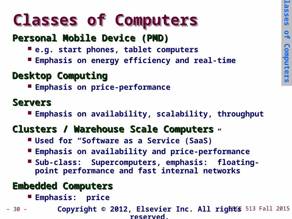
Classes of ComputersClasses of ComputersPersonal Mobile Device (PMD)Personal Mobile Device (PMD)

e.g. start phones, tablet computers Emphasis on energy efficiency and real-time

Desktop ComputingDesktop Computing Emphasis on price-performance

ServersServers Emphasis on availability, scalability, throughput

Clusters / Warehouse Scale ComputersClusters / Warehouse Scale Computers Used for “Software as a Service (SaaS)” Emphasis on availability and price-performance Sub-class: Supercomputers, emphasis: floating-point

performance and fast internal networks

Embedded ComputersEmbedded Computers Emphasis: price

Classes o

f Co

mp

uters


ParallelismParallelism

Classes of parallelism in applications:Classes of parallelism in applications: Data-Level Parallelism (DLP) Task-Level Parallelism (TLP)

Classes of architectural parallelism:Classes of architectural parallelism: Instruction-Level Parallelism (ILP) Vector architectures/Graphic Processor Units

(GPUs) Thread-Level Parallelism Request-Level Parallelism

Classes o

f Co

mp

uters

– 16 – CSCE 513 Fall 2015

Main MemoryMain Memory

DRAM – dynamic RAM – one transistor/capacitor per bitDRAM – dynamic RAM – one transistor/capacitor per bit

SRAM – static RAM – four to 6 transistors per bitSRAM – static RAM – four to 6 transistors per bit

DRAM density increases approx. 50% per year DRAM density increases approx. 50% per year

DRAM cycle time decreases slowly (DRAMs have DRAM cycle time decreases slowly (DRAMs have destructive read-out, like old core memories, and destructive read-out, like old core memories, and data row must be rewritten after each read) data row must be rewritten after each read)

DRAM must be refreshed every 2-8 ms DRAM must be refreshed every 2-8 ms

Memory bandwidth improves about twice the rate that Memory bandwidth improves about twice the rate that cycle time does due to improvements in signaling cycle time does due to improvements in signaling conventions and bus widthconventions and bus width


Trends in TechnologyTrends in Technology

Integrated circuit technologyIntegrated circuit technology Transistor density: 35%/year Die size: 10-20%/year Integration overall: 40-55%/year

DRAM capacity: 25-40%/year (slowing)DRAM capacity: 25-40%/year (slowing)

Flash capacity: 50-60%/yearFlash capacity: 50-60%/year 15-20X cheaper/bit than DRAM

Magnetic disk technology: 40%/yearMagnetic disk technology: 40%/year 15-25X cheaper/bit then Flash 300-500X cheaper/bit than DRAM

Tren

ds in

Tech

no

log

y


Power and EnergyPower and Energy

Problem: Get power in, get power outProblem: Get power in, get power out

Thermal Design Power (TDP)Thermal Design Power (TDP) Characterizes sustained power consumption Used as target for power supply and cooling

system Lower than peak power, higher than average

power consumption

Clock rate can be reduced dynamically to limit Clock rate can be reduced dynamically to limit power consumptionpower consumption

Energy per task is often a better measurementEnergy per task is often a better measurement

Tren

ds in

Po

wer an

d E

nerg

y


Dynamic Energy and PowerDynamic Energy and Power

Dynamic energyDynamic energy Transistor switch from 0 -> 1 or 1 -> 0 ½ x Capacitive load x Voltage2

Dynamic powerDynamic power ½ x Capacitive load x Voltage2 x Frequency

switched

Reducing clock rate reduces power, not energyReducing clock rate reduces power, not energy

Tren

ds in

Po

wer an

d E

nerg

y

– 20 – CSCE 513 Fall 2015

Energy Power exampleEnergy Power example

Example Some microprocessors today are designed to Example Some microprocessors today are designed to have adjustable voltage, so a 15% reduction in have adjustable voltage, so a 15% reduction in voltage may result in a 15% reduction in frequency. voltage may result in a 15% reduction in frequency. What would be the impact on dynamic energy and on What would be the impact on dynamic energy and on dynamic power? dynamic power?

Answer Since the capacitance is unchanged, the Answer Since the capacitance is unchanged, the answer for energy is the ratio of the voltages since answer for energy is the ratio of the voltages since the capacitance is unchanged:the capacitance is unchanged:

CAAQA


PowerPowerIntel 80386 consumed Intel 80386 consumed

~ 2 W~ 2 W

3.3 GHz Intel Core i7 3.3 GHz Intel Core i7 consumes 130 Wconsumes 130 W

Heat must be Heat must be dissipated from 1.5 dissipated from 1.5 x 1.5 cm chipx 1.5 cm chip

This is the limit of what This is the limit of what can be cooled by aircan be cooled by air

Tren

ds in

Po

wer an

d E

nerg

y


Reducing PowerReducing Power

Techniques for reducing power:Techniques for reducing power: Do nothing well Dynamic Voltage-Frequency Scaling Low power state for DRAM, disks Overclocking, turning off cores

Tren

ds in

Po

wer an

d E

nerg

y


Static PowerStatic Power

Static power consumptionStatic power consumption Currentstatic x Voltage Scales with number of transistors To reduce: power gating

Tren

ds in

Po

wer an

d E

nerg

y

– 24 – CSCE 513 Fall 2015

Intel Multi-core processors I-7 980Intel Multi-core processors I-7 980

Frequently Asked Questions: Intel® Multi-Core Frequently Asked Questions: Intel® Multi-Core Processor ArchitectureProcessor Architecture

Essential ConceptsEssential Concepts

The Move to Multi-Core Architecture ExplainedThe Move to Multi-Core Architecture Explained

How to Benefit from Multi-Core ArchitectureHow to Benefit from Multi-Core Architecture

Challenges in Multithreaded ProgrammingChallenges in Multithreaded Programming

How Intel Can HelpHow Intel Can Help

Additional ResourcesAdditional Resources

..

https://software.intel.com/en-us/articles/frequently-asked-questions-intel-multi-core-processor-architecture/

– 25 – CSCE 513 Fall 2015

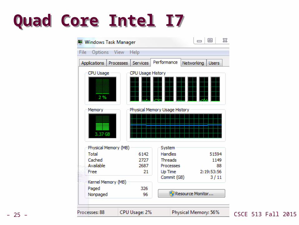
Quad Core Intel I7Quad Core Intel I7

– 26 – CSCE 513 Fall 2015Copyright © 2011, Elsevier Inc. All rights Reserved.

Figure 1.13 Photograph of an Intel Core i7 microprocessor die, which is evaluated in Chapters 2 through 5. The dimensions are 18.9 mm by 13.6 mm (257 mm2) in a 45 nm process. (Courtesy Intel.)


Figure 1.14 Floorplan of Core i7 die in Figure 1.13 on left with close-up of floorplan of second core on right.


Figure 1.15 This 300 mm wafer contains 280 full Sandy Bridge dies, each 20.7 by 10.5 mm in a 32 nm process. (Sandy Bridge is Intel’s successor to Nehalem used in the Core i7.) At 216 mm2, the formula for dies per wafer estimates 282. (Courtesy Intel.)

– 29 – CSCE 513 Fall 2015

Cost of IC’sCost of IC’s

Cost of IC = (Cost of die + cost of testing die + cost of packaging and final test) / (Final test yield)

Cost of die = Cost of wafer / (Dies per wafer * die yield)

Dies per wafer is wafer area divided by die area, less dies along the edge

= (wafer area) / (die area) - (wafer circumference) / (die diagonal)

Die yield = (Wafer yield) * ( 1 + (defects per unit area * die area/alpha) ) ** (-alpha)


Classes of ComputersClasses of ComputersPersonal Mobile Device (PMD)Personal Mobile Device (PMD)

e.g. start phones, tablet computers Emphasis on energy efficiency and real-time

Desktop ComputingDesktop Computing Emphasis on price-performance

ServersServers Emphasis on availability, scalability, throughput

Clusters / Warehouse Scale ComputersClusters / Warehouse Scale Computers Used for “Software as a Service (SaaS)” Emphasis on availability and price-performance Sub-class: Supercomputers, emphasis: floating-point

performance and fast internal networks

Embedded ComputersEmbedded Computers Emphasis: price

Classes o

f Co

mp

uters

– 31 – CSCE 513 Fall 2015

Performance MeasuresPerformance Measures

Response time (latency) -- time between start and Response time (latency) -- time between start and completion completion

Throughput (bandwidth) -- rate -- work done per unit Throughput (bandwidth) -- rate -- work done per unit time time

Speedup -- B is n times faster than ASpeedup -- B is n times faster than A Means exec_time_A/exec_time_B == rate_B/rate_A

Other important measures Other important measures

power (impacts battery life, cooling, packaging) power (impacts battery life, cooling, packaging)

RAS (reliability, availability, and serviceability) RAS (reliability, availability, and serviceability)

scalability (ability to scale up processors, memories, scalability (ability to scale up processors, memories, and I/O) and I/O)


Bandwidth and LatencyBandwidth and Latency

Bandwidth or throughputBandwidth or throughput Total work done in a given time 10,000-25,000X improvement for processors 300-1200X improvement for memory and disks

Latency or response timeLatency or response time Time between start and completion of an event 30-80X improvement for processors 6-8X improvement for memory and disks

Tren

ds in

Tech

no

log

y


Bandwidth and LatencyBandwidth and Latency

Log-log plot of bandwidth and latency milestones

Tren

ds in

Tech

no

log

y

– 34 – CSCE 513 Fall 2015

Measuring Performance Measuring Performance

Time is the measure of computer performance Time is the measure of computer performance

Elapsed time = program execution + I/O + wait -- Elapsed time = program execution + I/O + wait -- important to user important to user

Execution time = user time + system time (but OS self Execution time = user time + system time (but OS self measurement may be inaccurate) measurement may be inaccurate)

CPU performance = user time on unloaded system -- CPU performance = user time on unloaded system -- important to architect important to architect

– 35 – CSCE 513 Fall 2015

Real PerformanceReal Performance

Benchmark suitesBenchmark suites

Performance is the result of executing a workload on a Performance is the result of executing a workload on a configuration configuration

Workload = program + input Workload = program + input

Configuration = CPU + cache + memory + I/O + OS + Configuration = CPU + cache + memory + I/O + OS + compiler + optimizations compiler + optimizations

compiler optimizations can make a huge difference! compiler optimizations can make a huge difference!

– 36 – CSCE 513 Fall 2015

Benchmark SuitesBenchmark Suites

Whetstone (1976) -- designed to simulate arithmetic-Whetstone (1976) -- designed to simulate arithmetic-intensive scientific programs. intensive scientific programs.

Dhrystone (1984) -- designed to simulate systems Dhrystone (1984) -- designed to simulate systems programming applications. Structure, pointer, and programming applications. Structure, pointer, and string operations are based on observed string operations are based on observed frequencies, as well as types of operand access frequencies, as well as types of operand access (global, local, parameter, and constant). (global, local, parameter, and constant).

PC Benchmarks – aimed at simulating real PC Benchmarks – aimed at simulating real environmentsenvironments Business Winstone – navigator + Office Apps CC Winstone – Winbench -

– 37 – CSCE 513 Fall 2015

Comparing PerformanceComparing Performance

Total execution time (implies equal mix in workload) Total execution time (implies equal mix in workload) Just add up the times

Arithmetic average of execution time Arithmetic average of execution time To get more accurate picture, compute the average of

several runs of a program

Weighted execution time (weighted arithmetic mean) Weighted execution time (weighted arithmetic mean) Program p1 makes up 25% of workload (estimated), P2 75%

then use weighted average

– 38 – CSCE 513 Fall 2015

Comparing Performance cont.Comparing Performance cont.

Normalized execution time or speedup (normalize Normalized execution time or speedup (normalize relative to reference machine and take average) relative to reference machine and take average)

SPEC benchmarks (base time a SPARCstation)SPEC benchmarks (base time a SPARCstation)

Arithmetic mean sensitive to reference machine choice Arithmetic mean sensitive to reference machine choice

Geometric mean consistent but cannot predict Geometric mean consistent but cannot predict execution time execution time Nth root of the product of execution time ratios

Combining samples

– 39 – CSCE 513 Fall 2015

– 40 – CSCE 513 Fall 2015

Improve Performance byImprove Performance by

changing the changing the algorithm data structures programming language compiler compiler optimization flags OS parameters

improving locality of memory or I/O accesses improving locality of memory or I/O accesses

overlapping I/O overlapping I/O

on multiprocessors, you can improve performance by on multiprocessors, you can improve performance by avoiding cache coherency problems (e.g., false avoiding cache coherency problems (e.g., false sharing) and synchronization problems sharing) and synchronization problems

– 41 – CSCE 513 Fall 2015

Amdahl’s LawAmdahl’s Law

Speedup =Speedup =

(performance of entire task not using enhancement(performance of entire task not using enhancement))

(performance of entire task using enhancement)(performance of entire task using enhancement)

AlternativelyAlternatively

Speedup = Speedup =

(execution time without enhancement) / (execution (execution time without enhancement) / (execution time with enhancement)time with enhancement)

– 42 – CSCE 513 Fall 2015

– 43 – CSCE 513 Fall 2015

Performance MeasuresPerformance Measures

Response time (latency) -- time between start and completion Response time (latency) -- time between start and completion

Throughput (bandwidth) -- rate -- work done per unit time Throughput (bandwidth) -- rate -- work done per unit time

Speedup = Speedup =

(execution time without enhance.) / (execution time with enhance.)(execution time without enhance.) / (execution time with enhance.)

= time= timewo enhancementwo enhancement) / (time) / (timewith enhancementwith enhancement))

Processor Speed – e.g. 1GHzProcessor Speed – e.g. 1GHz

When does it matter? When does it matter?

When does it not?When does it not?

– 44 – CSCE 513 Fall 2015

MIPS and MFLOPSMIPS and MFLOPS

MIPS (Millions of Instructions per second)MIPS (Millions of Instructions per second)

= (instruction count) / (execution time * 10= (instruction count) / (execution time * 1066)) Problem1 depends on the instruction set (ISA) Problem2 varies with different programs on the same machine

MFLOPS (mega-flops where a flop is a floating point operation)MFLOPS (mega-flops where a flop is a floating point operation)

= (floating point instruction count) / (execution time * 10= (floating point instruction count) / (execution time * 1066)) Problem1 depends on the instruction set (ISA) Problem2 varies with different programs on the same machine

– 45 – CSCE 513 Fall 2015

Amdahl’s Law revisitedAmdahl’s Law revisited

Speedup = Speedup =

(execution time without enhance.) / (execution time with (execution time without enhance.) / (execution time with enhance.)enhance.)

= (time without) / (time with) = T= (time without) / (time with) = Twowo / T / Twithwith

NotesNotes

1.1. The enhancement will be used only a portion of the time.The enhancement will be used only a portion of the time.

2.2. If it will be rarely used then why bother trying to improve itIf it will be rarely used then why bother trying to improve it

3.3. Focus on the improvements that have the highest fraction of Focus on the improvements that have the highest fraction of use time denoted Fractionuse time denoted Fractionenhancedenhanced. .

4.4. Note FractionNote Fractionenhancedenhanced is always less than 1. is always less than 1.

Then Then

– 46 – CSCE 513 Fall 2015

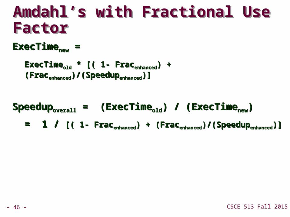
Amdahl’s with Fractional Use FactorAmdahl’s with Fractional Use Factor

ExecTimeExecTimenewnew = =

ExecTimeExecTimeoldold * [( 1- Frac * [( 1- Fracenhancedenhanced) + (Frac) + (Fracenhancedenhanced)/(Speedup)/(Speedupenhancedenhanced)])]

SpeedupSpeedupoveralloverall = (ExecTime = (ExecTimeoldold) / (ExecTime) / (ExecTimenewnew))

= 1 / = 1 / [( 1- Frac[( 1- Fracenhancedenhanced) + (Frac) + (Fracenhancedenhanced)/(Speedup)/(Speedupenhancedenhanced)])]

– 47 – CSCE 513 Fall 2015

Amdahl’s with Fractional Use FactorAmdahl’s with Fractional Use Factor

Example:Example: Suppose we are considering an enhancement to Suppose we are considering an enhancement to a web server. The enhanced CPU is 10 times faster on a web server. The enhanced CPU is 10 times faster on computation but the same speed on I/O. Suppose also computation but the same speed on I/O. Suppose also that 60% of the time is waiting on I/Othat 60% of the time is waiting on I/O

FracFracenhancedenhanced = .4 = .4

SpeedupSpeedupenhancedenhanced = 10 = 10

SpeedupSpeedupoveralloverall = =

= 1 / = 1 / [( 1- Frac[( 1- Fracenhancedenhanced) + (Frac) + (Fracenhancedenhanced)/(Speedup)/(Speedupenhancedenhanced)])]

==

– 48 – CSCE 513 Fall 2015

Graphics Square Root Enhancement p 42Graphics Square Root Enhancement p 42

– 49 – CSCE 513 Fall 2015

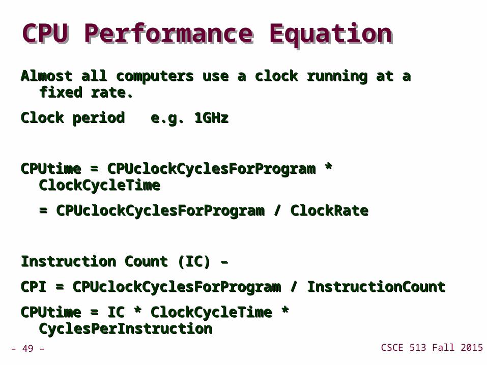
CPU Performance EquationCPU Performance Equation

Almost all computers use a clock running at a fixed Almost all computers use a clock running at a fixed rate.rate.

Clock period e.g. 1GHzClock period e.g. 1GHz

CPUtime = CPUclockCyclesForProgram * CPUtime = CPUclockCyclesForProgram * ClockCycleTimeClockCycleTime

= CPUclockCyclesForProgram / ClockRate= CPUclockCyclesForProgram / ClockRate

Instruction Count (IC) – Instruction Count (IC) –

CPI = CPUclockCyclesForProgram / InstructionCountCPI = CPUclockCyclesForProgram / InstructionCount

CPUtime = IC * ClockCycleTime * CyclesPerInstructionCPUtime = IC * ClockCycleTime * CyclesPerInstruction

– 50 – CSCE 513 Fall 2015

CPU Performance EquationCPU Performance Equation

CPUtime = IC * ClockCycleTime * CyclesPerInstructionCPUtime = IC * ClockCycleTime * CyclesPerInstruction

CPUtimeCPUtime

– 51 – CSCE 513 Fall 2015

Principle of LocalityPrinciple of Locality

Rule of thumb – Rule of thumb –

A program spends 90% of its execution time in only A program spends 90% of its execution time in only 10% of the code.10% of the code.

So what do you try to optimize?So what do you try to optimize?

Locality of memory referencesLocality of memory references

Temporal localityTemporal locality

Spatial localitySpatial locality

– 52 – CSCE 513 Fall 2015

Taking Advantage of ParallelismTaking Advantage of Parallelism

Logic parallelism – carry lookahead adderLogic parallelism – carry lookahead adder

Word parallelism – SIMDWord parallelism – SIMD

Instruction pipelining – overlap fetch and executeInstruction pipelining – overlap fetch and execute

Multithreads – executing independent instructions at Multithreads – executing independent instructions at the same timethe same time

Speculative execution - Speculative execution -

– 53 – CSCE 513 Fall 2015

Homework Set #1Homework Set #1

1.1. 1.21.2

2.2. 1.71.7

3.3. 1.81.8

4.4. 1.91.9

– 54 – CSCE 513 Fall 2015

ISA – Example MIPs/ IA32ISA – Example MIPs/ IA32


Figure 1.6 MIPS64 instruction set architecture formats. All instructions are 32 bits long. The R format is for integer register-to-register operations, such as DADDU, DSUBU, and so on. The I format is for data transfers, branches, and

immediate instructions, such as LD, SD, BEQZ, and DADDIs. The J format is for jumps, the FR format for floating-point operations, and the FI format for floating-point branches.

Documents

Lecture 1 Overview of Computer Architecture TopicsOverview Readings: Chapter 1 August 24, 2015 CSCE 513 Computer Architecture