Lecture ATP

1

Intro to ATP Spring 2009

UIECE 529Lecture 4

1

Installing ATP:

• Minimum to Download» Mingw version of ATP» ATPDraw -- latest version or latest patch

– Presently Atpdraw55.zip» PlotXY

• Installation is less straightforward.


UIECE 529Lecture 4

2

Installing ATPDraw

• Installation is fairly easy• Default installation path “Program Files”• The space in the file name can create

problems running ATP from ATPDraw» Install it somewhere else. I normally install

in “C:\tools\prog\ATPDraw”• Install program creates shortcut in the

start menu, but not very cleanly

2


UIECE 529Lecture 4

3

Running ATP from ATPDraw

• Still need a copy of ATP• Licensed users can get other versions• Follow installation directions for yours• ATPDraw calls ATP from a DOS Batch

file (extension *.bat)• Passes full path to file when calls ATP


UIECE 529Lecture 4

4

Sample Batch File

• The following batch file is for Ming32 ATPSET GNUDIR=C:\tools\prog\atp\SET PATH=C:\tools\prog\atp;"%PATH%”tpbig both %1 s -r

The first line defines variable GNUDIR» Different ATP versions use different name» Sets program working environment» The final “\” is important

3


UIECE 529Lecture 4

5

Sample Batch File (cont.)» Second line adds executable to your search

path (not needed if set this at boot time)» The next line calls ATP itself

– tpbig both %1 s -R

» “both” tells program to write error messages to screen and to file (useful for debugging)

» Could also set “disk” to only do disk file or leave blank for no message

» First “%1” is input data file from ATPDraw


UIECE 529Lecture 4

6

Sample Batch File (cont.)» The “s” is to create appropriate output file. » “-R” tells ATP overwrite existing output file if one

exists• This bat file will let you run ATP, and all of

the support program (line constants etc)

4


UIECE 529Lecture 4

7

Editing “startup”

• ATP reads a file called “startup”» Resides in same directory as tpbig» Sets variables for the program

• A few suggested changes from default» Change PL4 file format to work with PlotXY» Ignore blank lines


UIECE 529Lecture 4

8

Editing “startup”

• ATP reads a file called “startup”» Resides in same directory as tpbig» Sets variables for the program

• A few suggested changes from default» Change PL4 file format to work with PlotXY

– NOBLAN set to 0– NEWPL4 set to 1

5


UIECE 529Lecture 4

9

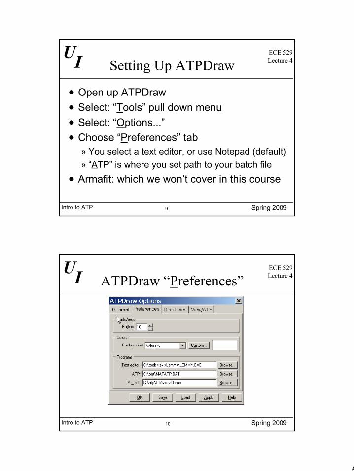
Setting Up ATPDraw

• Open up ATPDraw• Select: “Tools” pull down menu• Select: “Options...”• Choose “Preferences” tab

» You select a text editor, or use Notepad (default)» “ATP” is where you set path to your batch file

• Armafit: which we won’t cover in this course


UIECE 529Lecture 4

10

ATPDraw “Preferences”

6


UIECE 529Lecture 4

11

Further Settings

• The “Directories” tab settings are ok» Problems with “lost” help files though

• However, you do want changes in the View/ATP tab» Select “Edit settings” tab» You may want to change some of the

default settings. However, you can change any of these for a specific data file


UIECE 529Lecture 4

12

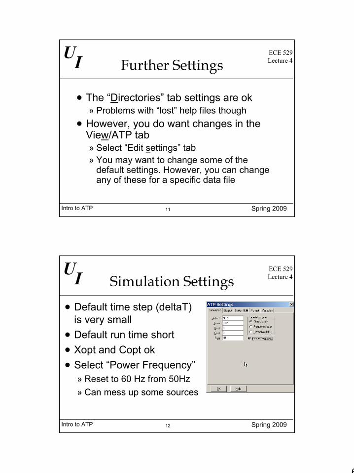
Simulation Settings

• Default time step (deltaT) is very small

• Default run time short• Xopt and Copt ok• Select “Power Frequency”

» Reset to 60 Hz from 50Hz» Can mess up some sources

7


UIECE 529Lecture 4

13

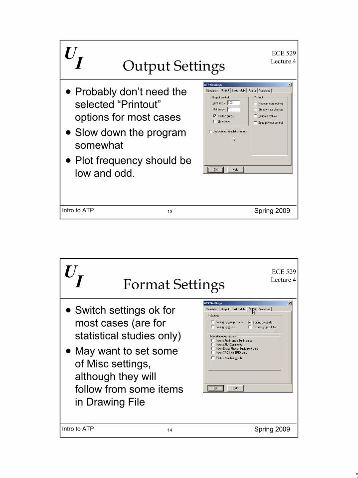
Output Settings

• Probably don’t need the selected “Printout”options for most cases

• Slow down the program somewhat

• Plot frequency should be low and odd.


UIECE 529Lecture 4

14

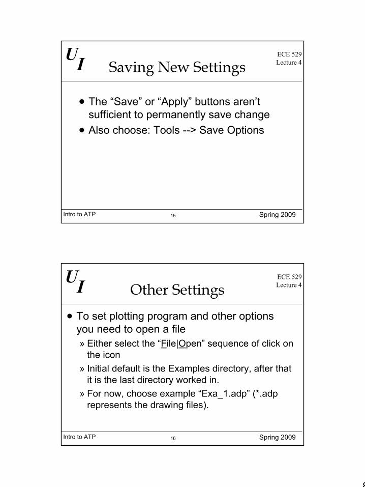
Format Settings

• Switch settings ok for most cases (are for statistical studies only)

• May want to set some of Misc settings, although they will follow from some items in Drawing File

8


UIECE 529Lecture 4

15

Saving New Settings

• The “Save” or “Apply” buttons aren’t sufficient to permanently save change

• Also choose: Tools --> Save Options


UIECE 529Lecture 4

16

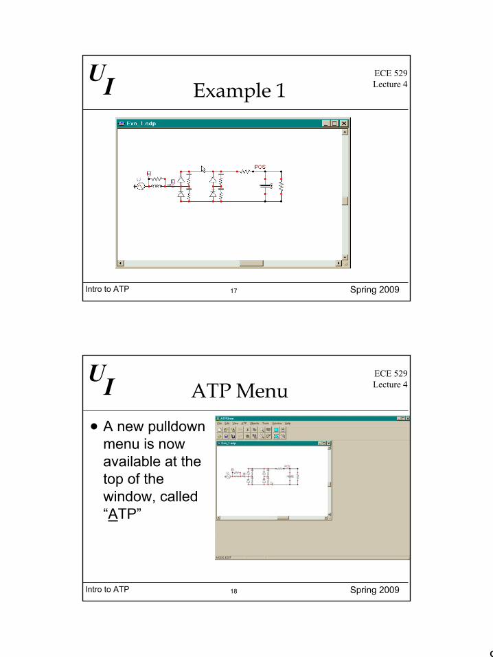
Other Settings

• To set plotting program and other options you need to open a file» Either select the “File|Open” sequence of click on

the icon» Initial default is the Examples directory, after that

it is the last directory worked in.» For now, choose example “Exa_1.adp” (*.adp

represents the drawing files).

9


UIECE 529Lecture 4

17

Example 1


UIECE 529Lecture 4

18

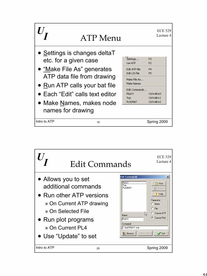
ATP Menu

• A new pulldown menu is now available at the top of the window, called “ATP”

10


UIECE 529Lecture 4

19

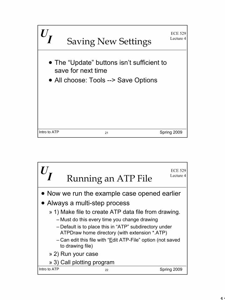
ATP Menu

• Settings is changes deltaT etc. for a given case

• “Make File As” generates ATP data file from drawing

• Run ATP calls your bat file• Each “Edit” calls text editor• Make Names, makes node

names for drawing


UIECE 529Lecture 4

20

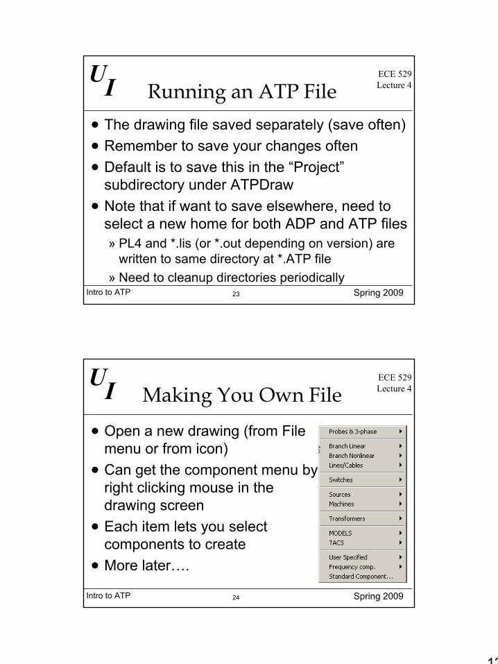
Edit Commands

• Allows you to set additional commands

• Run other ATP versions» On Current ATP drawing» On Selected File

• Run plot programs » On Current PL4

• Use “Update” to set

11


UIECE 529Lecture 4

21

Saving New Settings

• The “Update” buttons isn’t sufficient to save for next time

• All choose: Tools --> Save Options


UIECE 529Lecture 4

22

Running an ATP File• Now we run the example case opened earlier• Always a multi-step process

» 1) Make file to create ATP data file from drawing. – Must do this every time you change drawing– Default is to place this in “ATP” subdirectory under

ATPDraw home directory (with extension *.ATP)– Can edit this file with “Edit ATP-File” option (not saved

to drawing file)» 2) Run your case» 3) Call plotting program

12


UIECE 529Lecture 4

23

Running an ATP File• The drawing file saved separately (save often)• Remember to save your changes often• Default is to save this in the “Project”

subdirectory under ATPDraw• Note that if want to save elsewhere, need to

select a new home for both ADP and ATP files» PL4 and *.lis (or *.out depending on version) are

written to same directory at *.ATP file» Need to cleanup directories periodically


UIECE 529Lecture 4

24

Making You Own File

• Open a new drawing (from File menu or from icon)

• Can get the component menu by right clicking mouse in the drawing screen

• Each item lets you select components to create

• More later….

13


UIECE 529Lecture 4

25

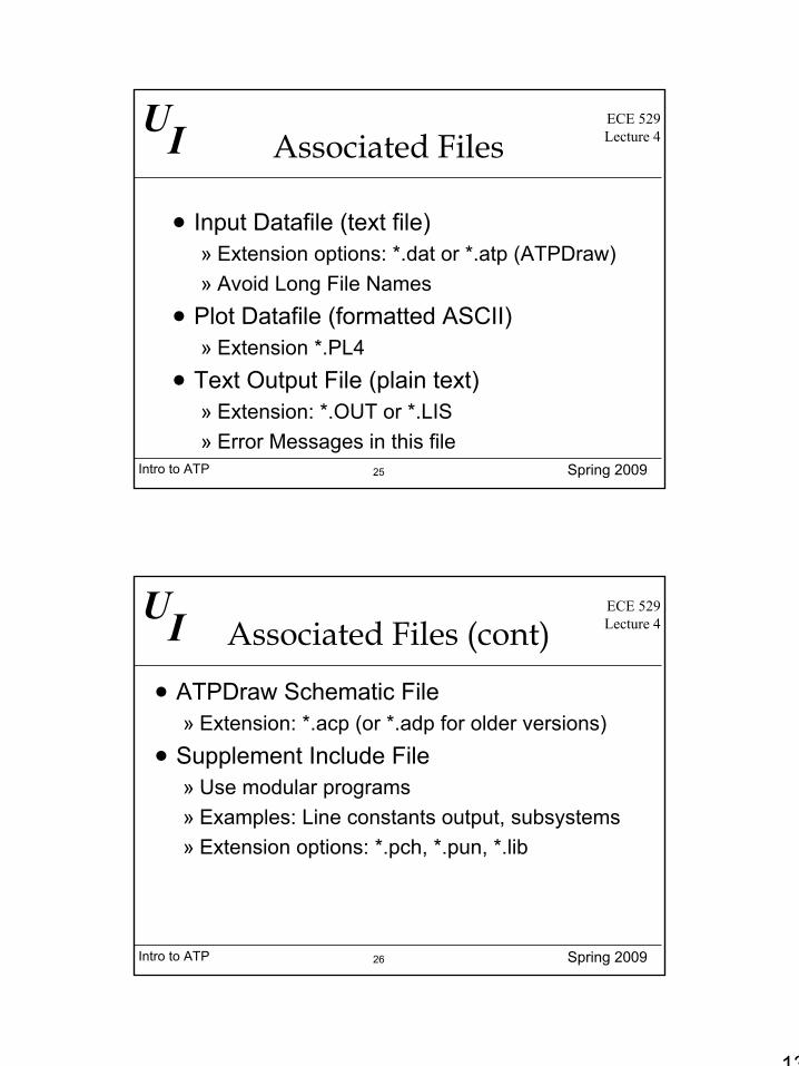
Associated Files

• Input Datafile (text file)» Extension options: *.dat or *.atp (ATPDraw)» Avoid Long File Names

• Plot Datafile (formatted ASCII)» Extension *.PL4

• Text Output File (plain text)» Extension: *.OUT or *.LIS» Error Messages in this file


UIECE 529Lecture 4

26

Associated Files (cont)

• ATPDraw Schematic File» Extension: *.acp (or *.adp for older versions)

• Supplement Include File» Use modular programs» Examples: Line constants output, subsystems» Extension options: *.pch, *.pun, *.lib

14


UIECE 529Lecture 4

27

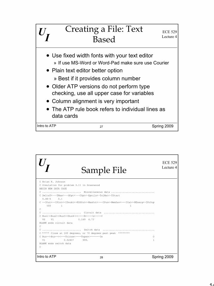
Creating a File: Text Based

• Use fixed width fonts with your text editor» If use MS-Word or Word-Pad make sure use Courier

• Plain text editor better option» Best if it provides column number

• Older ATP versions do not perform type checking, use all upper case for variables

• Column alignment is very important • The ATP rule book refers to individual lines as

data cards


UIECE 529Lecture 4

28

Sample FileC Brian K. JohnsonC Simulation for problem 3.11 in GreenwoodBEGIN NEW DATA CASEC ........................... Miscellaneous data ..............................C DeltaT<---TMax<---XOpt<---COpt<-Epsiln<-TolMat<-TStart5.0E-5 0.1

C --IOut<--IPlot<-IDoubl<-KSSOut<-MaxOut<---IPun<-MemSav<---ICat<-NEnerg<-IPrSup500 1 1

CC ........................... Circuit data ...................................C Bus1->Bus2->Bus3->Bus4-><----R<----L<----CVS V1 0.149 4.73

BLANK ends circuit dataCC ........................... Switch data ....................................C ***** Close at 160 degrees, or 70 degrees past peak ********C Bus-->Bus--><---Tclose<----Topen<-------Ie OV1 0.02407 999. 1

BLANK ends switch dataC

15


UIECE 529Lecture 4

29

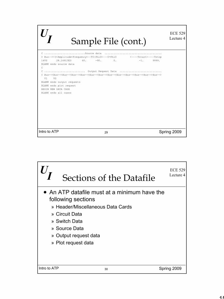
Sample File (cont.)C ...........................Source data ......................................C Bus--><I<Amplitude<Frequency<--T0|Phi0<---0=Phi0 <----Tstart<----Tstop14VS 28.16913E3 60. -90. 0. -1. 9999.BLANK ends source dataCC ........................... Output Request Data ............................C Bus-->Bus-->Bus-->Bus-->Bus-->Bus-->Bus-->Bus-->Bus-->Bus-->Bus-->Bus-->Bus-->V1 VS

BLANK ends output requestsBLANK ends plot requestBEGIN NEW DATA CASEBLANK ends all cases


UIECE 529Lecture 4

30

Sections of the Datafile• An ATP datafile must at a minimum have the

following sections» Header/Miscellaneous Data Cards» Circuit Data» Switch Data» Source Data» Output request data» Plot request data

16


UIECE 529Lecture 4

31

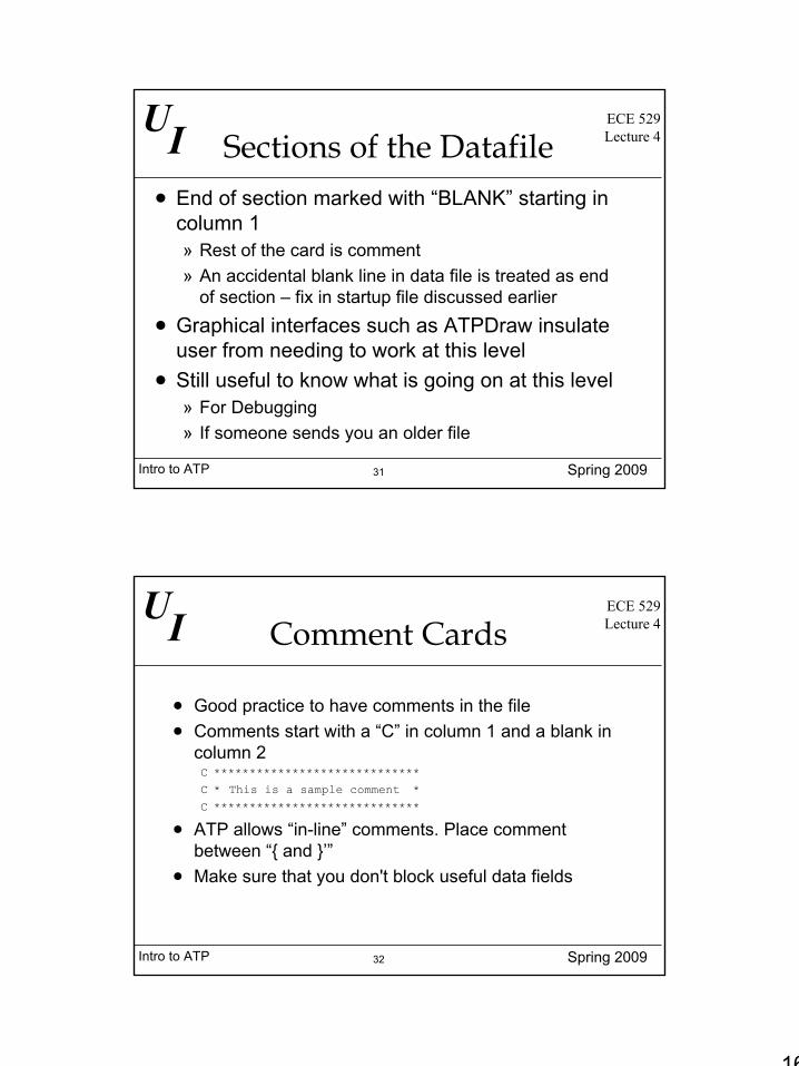
Sections of the Datafile• End of section marked with “BLANK” starting in

column 1» Rest of the card is comment» An accidental blank line in data file is treated as end

of section – fix in startup file discussed earlier• Graphical interfaces such as ATPDraw insulate

user from needing to work at this level• Still useful to know what is going on at this level

» For Debugging» If someone sends you an older file


UIECE 529Lecture 4

32

Comment Cards

• Good practice to have comments in the file• Comments start with a “C” in column 1 and a blank in

column 2C *****************************C * This is a sample comment *

C *****************************

• ATP allows “in-line” comments. Place comment between “{ and }’”

• Make sure that you don't block useful data fields

17


UIECE 529Lecture 4

33

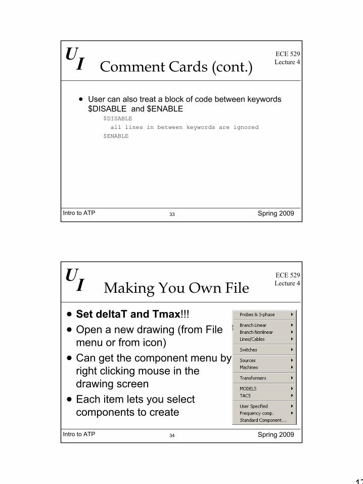
Comment Cards (cont.)

• User can also treat a block of code between keywords $DISABLE and $ENABLE

$DISABLE

all lines in between keywords are ignored

$ENABLE


UIECE 529Lecture 4

34

Making You Own File

• Set deltaT and Tmax!!!• Open a new drawing (from File

menu or from icon)• Can get the component menu by

right clicking mouse in the drawing screen

• Each item lets you select components to create

18


UIECE 529Lecture 4

35

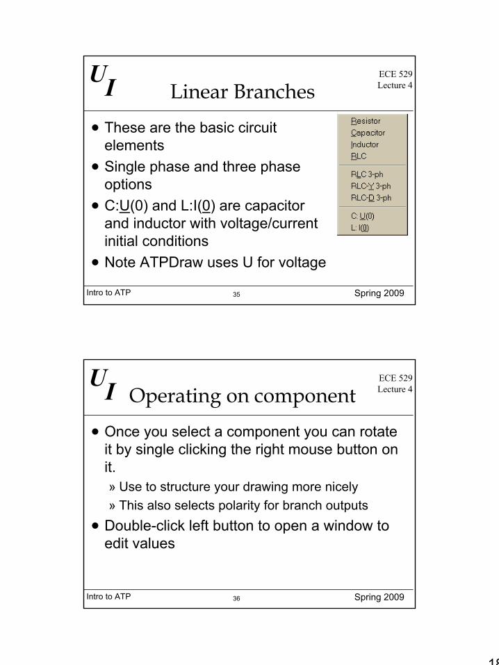
Linear Branches

• These are the basic circuit elements

• Single phase and three phase options

• C:U(0) and L:I(0) are capacitor and inductor with voltage/current initial conditions

• Note ATPDraw uses U for voltage


UIECE 529Lecture 4

36

Operating on component

• Once you select a component you can rotate it by single clicking the right mouse button on it. » Use to structure your drawing more nicely» This also selects polarity for branch outputs

• Double-click left button to open a window to edit values

19


UIECE 529Lecture 4

37

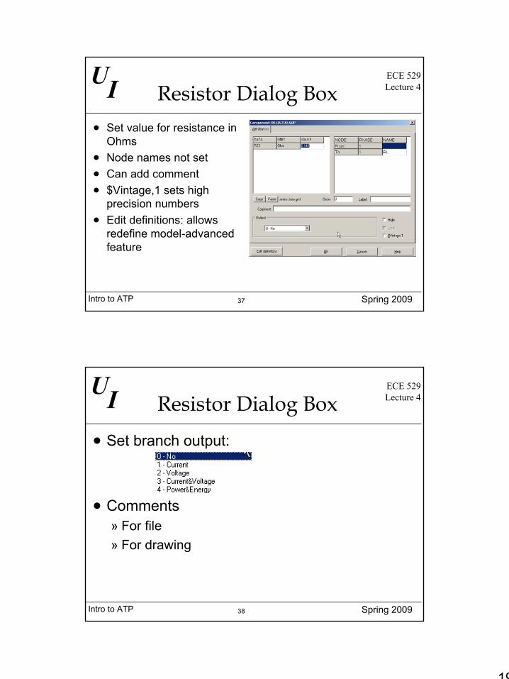
Resistor Dialog Box• Set value for resistance in

Ohms• Node names not set• Can add comment• $Vintage,1 sets high

precision numbers• Edit definitions: allows

redefine model-advanced feature


UIECE 529Lecture 4

38

Resistor Dialog Box

• Set branch output:

• Comments» For file» For drawing

20


UIECE 529Lecture 4

39

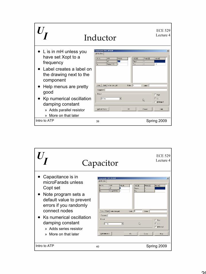
Inductor• L is in mH unless you

have set Xopt to a frequency

• Label creates a label on the drawing next to the component

• Help menus are pretty good

• Kp numerical oscillation damping constant» Adds parallel resistor» More on that later


UIECE 529Lecture 4

40

Capacitor• Capacitance is in

microFarads unless Copt set

• Note program sets a default value to prevent errors if you randomly connect nodes

• Ks numerical oscillation damping constant» Adds series resistor» More on that later

21


UIECE 529Lecture 4

41

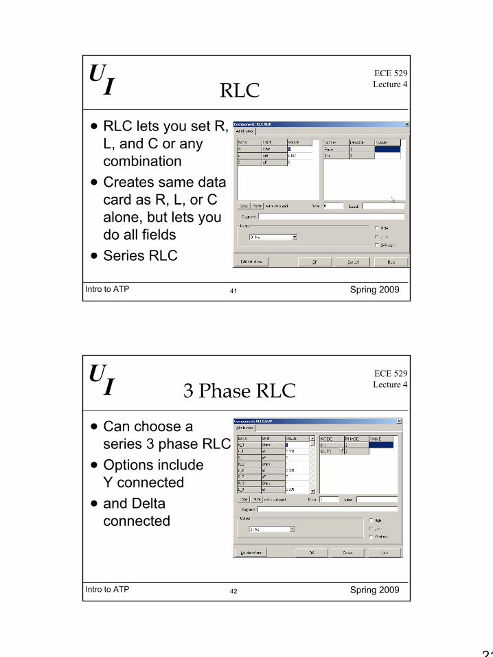
RLC

• RLC lets you set R, L, and C or any combination

• Creates same data card as R, L, or C alone, but lets you do all fields

• Series RLC


UIECE 529Lecture 4

42

3 Phase RLC

• Can choose a series 3 phase RLC

• Options include Y connected

• and Delta connected

22


UIECE 529Lecture 4

43

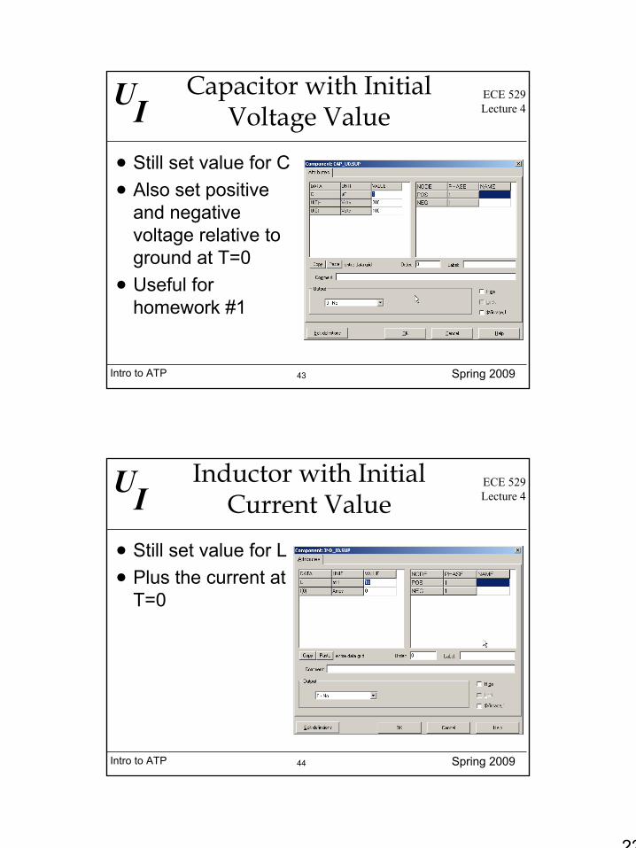
Capacitor with Initial Voltage Value

• Still set value for C• Also set positive

and negative voltage relative to ground at T=0

• Useful for homework #1


UIECE 529Lecture 4

44

Inductor with Initial Current Value

• Still set value for L• Plus the current at

T=0

23


UIECE 529Lecture 4

45

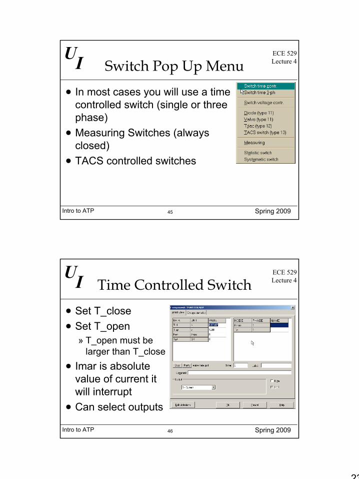
Switch Pop Up Menu

• In most cases you will use a time controlled switch (single or three phase)

• Measuring Switches (always closed)

• TACS controlled switches


UIECE 529Lecture 4

46

Time Controlled Switch

• Set T_close• Set T_open

» T_open must be larger than T_close

• Imar is absolute value of current it will interrupt

• Can select outputs

24


UIECE 529Lecture 4

47

Three Phase Switch


UIECE 529Lecture 4

48

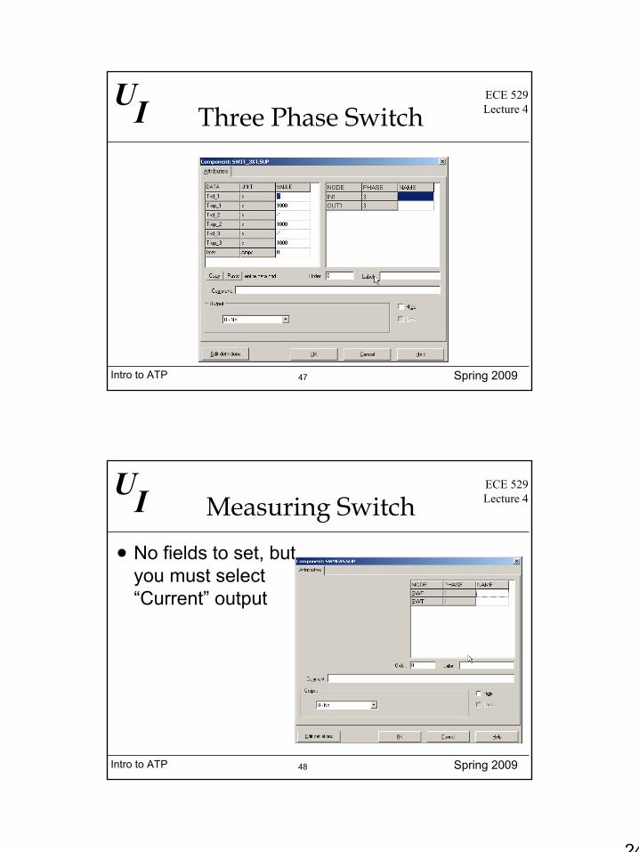
Measuring Switch

• No fields to set, but you must select “Current” output

25


UIECE 529Lecture 4

49

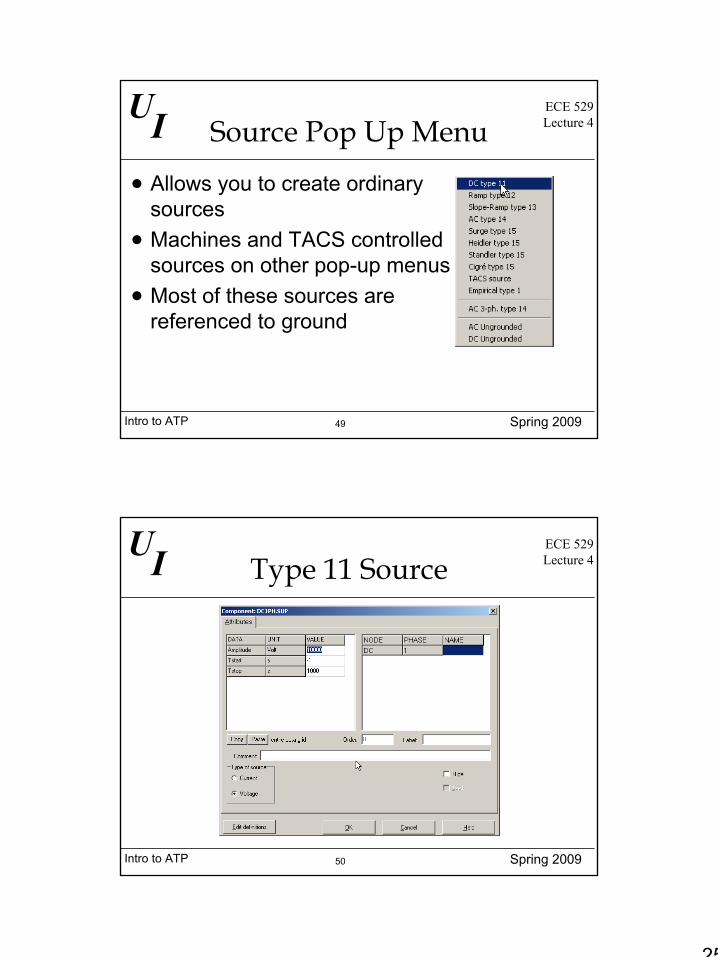
Source Pop Up Menu

• Allows you to create ordinary sources

• Machines and TACS controlled sources on other pop-up menus

• Most of these sources are referenced to ground


UIECE 529Lecture 4

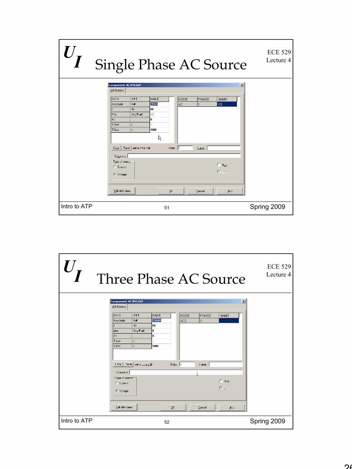
50

Type 11 Source

26


UIECE 529Lecture 4

51

Single Phase AC Source


UIECE 529Lecture 4

52

Three Phase AC Source

27


UIECE 529Lecture 4

53

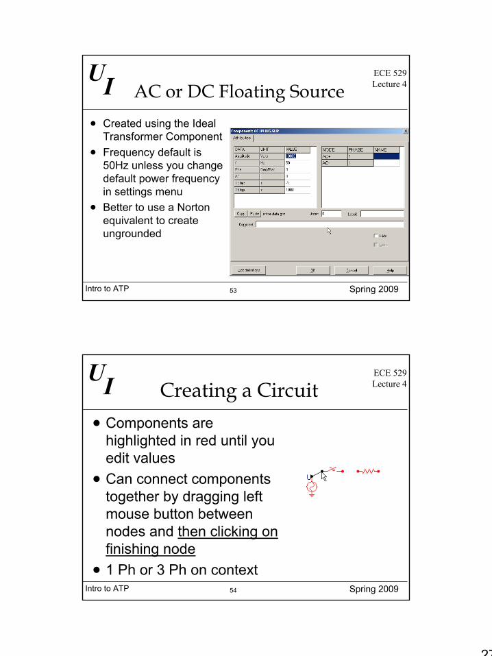
AC or DC Floating Source• Created using the Ideal

Transformer Component• Frequency default is

50Hz unless you change default power frequency in settings menu

• Better to use a Norton equivalent to create ungrounded


UIECE 529Lecture 4

54

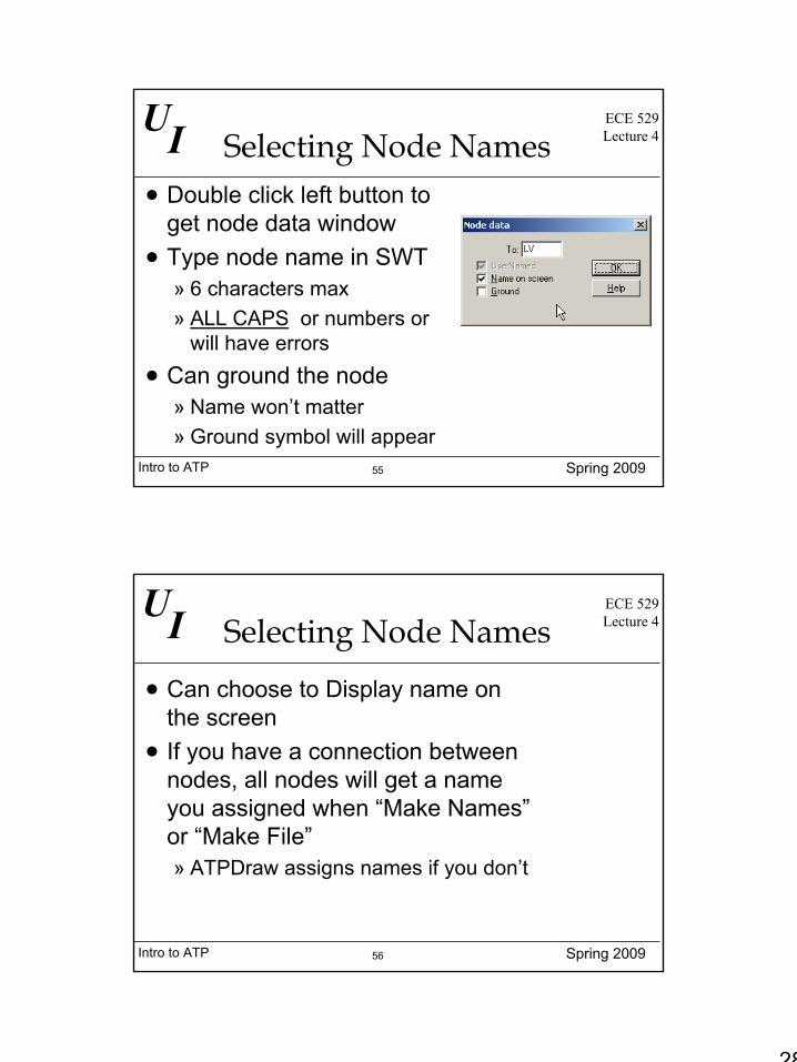
Creating a Circuit• Components are

highlighted in red until you edit values

• Can connect components together by dragging left mouse button between nodes and then clicking on finishing node

• 1 Ph or 3 Ph on context

28


UIECE 529Lecture 4

55

Selecting Node Names• Double click left button to

get node data window• Type node name in SWT

» 6 characters max » ALL CAPS or numbers or

will have errors• Can ground the node

» Name won’t matter» Ground symbol will appear


UIECE 529Lecture 4

56

Selecting Node Names

• Can choose to Display name on the screen

• If you have a connection between nodes, all nodes will get a name you assigned when “Make Names”or “Make File”» ATPDraw assigns names if you don’t

29


UIECE 529Lecture 4

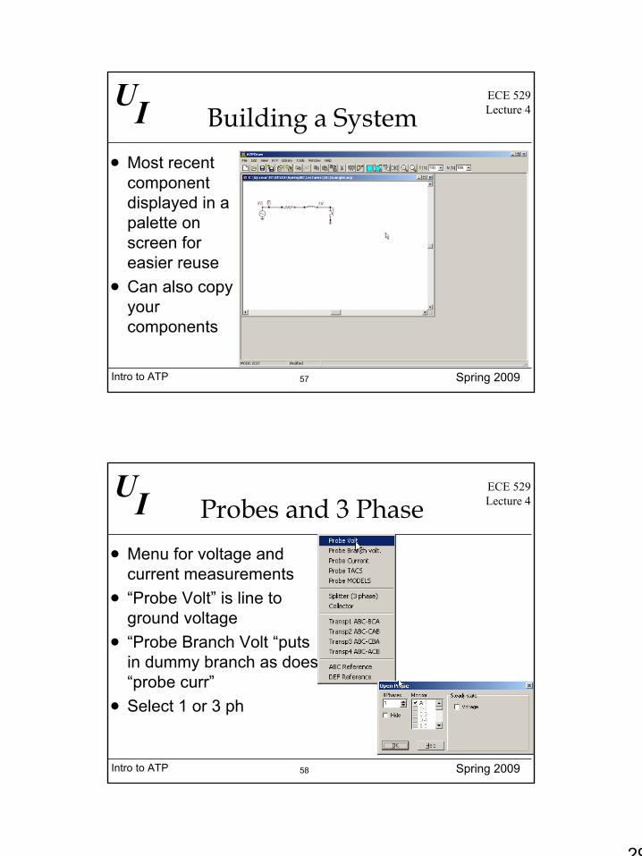
57

Building a System• Most recent

component displayed in a palette on screen for easier reuse

• Can also copy your components


UIECE 529Lecture 4

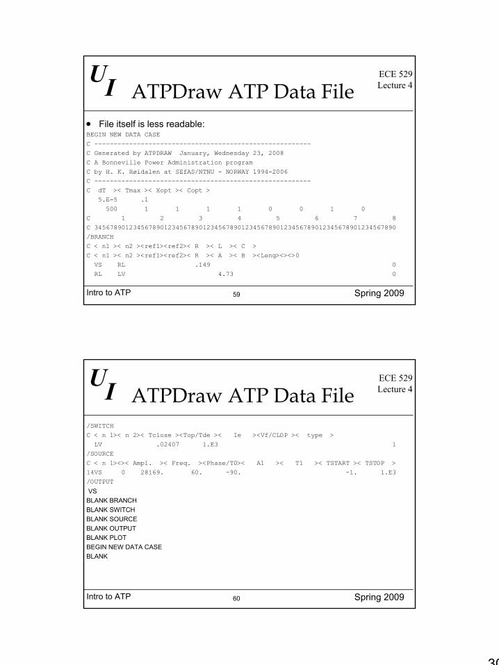
58

Probes and 3 Phase• Menu for voltage and

current measurements• “Probe Volt” is line to

ground voltage• “Probe Branch Volt “puts

in dummy branch as does “probe curr”

• Select 1 or 3 ph

30


UIECE 529Lecture 4

59

ATPDraw ATP Data File• File itself is less readable:BEGIN NEW DATA CASEC --------------------------------------------------------C Generated by ATPDRAW January, Wednesday 23, 2008C A Bonneville Power Administration programC by H. K. Høidalen at SEfAS/NTNU - NORWAY 1994-2006C --------------------------------------------------------C dT >< Tmax >< Xopt >< Copt >

5.E-5 .1 500 1 1 1 1 0 0 1 0

C 1 2 3 4 5 6 7 8C 345678901234567890123456789012345678901234567890123456789012345678901234567890/BRANCHC < n1 >< n2 ><ref1><ref2>< R >< L >< C >C < n1 >< n2 ><ref1><ref2>< R >< A >< B ><Leng><><>0VS RL .149 0RL LV 4.73 0


UIECE 529Lecture 4

60

ATPDraw ATP Data File/SWITCHC < n 1>< n 2>< Tclose ><Top/Tde >< Ie ><Vf/CLOP >< type >LV .02407 1.E3 1

/SOURCEC < n 1><>< Ampl. >< Freq. ><Phase/T0>< A1 >< T1 >< TSTART >< TSTOP >14VS 0 28169. 60. -90. -1. 1.E3/OUTPUT

VS BLANK BRANCHBLANK SWITCHBLANK SOURCEBLANK OUTPUTBLANK PLOTBEGIN NEW DATA CASEBLANK

31


UIECE 529Lecture 4

61

Lumped Parameter Lines: ATP

• All three model coupled branches

• Can do varying number of phases (up to 6)

• Can do several hundred phases when create by hand


UIECE 529Lecture 4

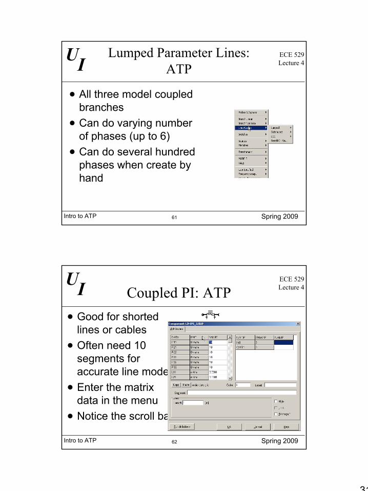
62

Coupled PI: ATP• Good for shorted

lines or cables• Often need 10

segments for accurate line model

• Enter the matrix data in the menu

• Notice the scroll bar

32


UIECE 529Lecture 4

63

Coupled RL: ATP• Enter using coupled-pi• Don’t enter capacitance values• Use for network equivalent


UIECE 529Lecture 4

64

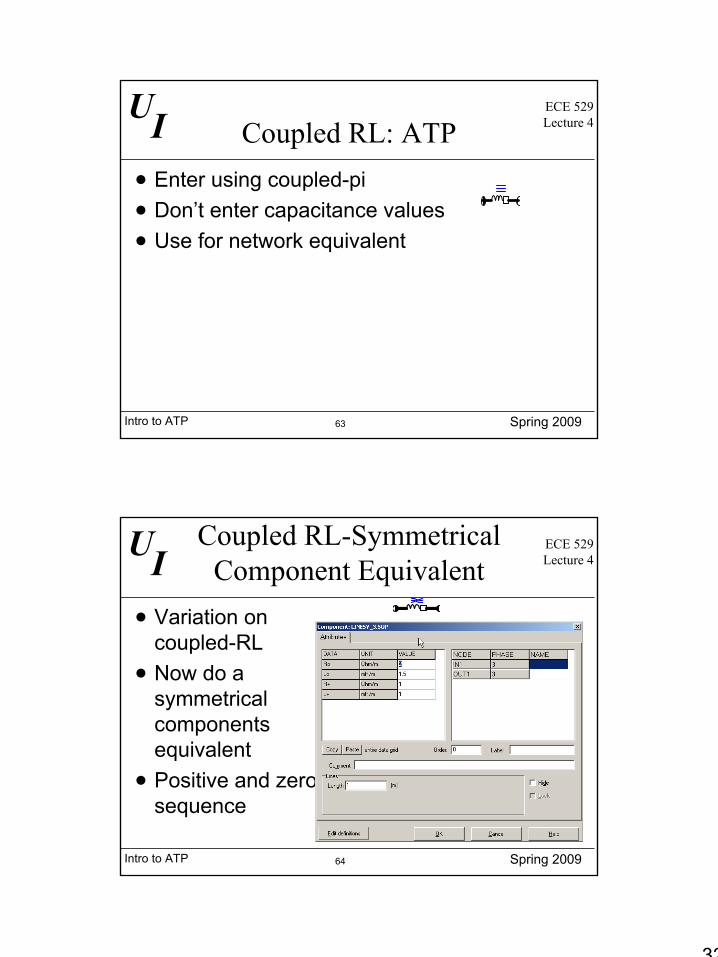
Coupled RL-Symmetrical Component Equivalent

• Variation on coupled-RL

• Now do a symmetrical components equivalent

• Positive and zero sequence

33


UIECE 529Lecture 4

65

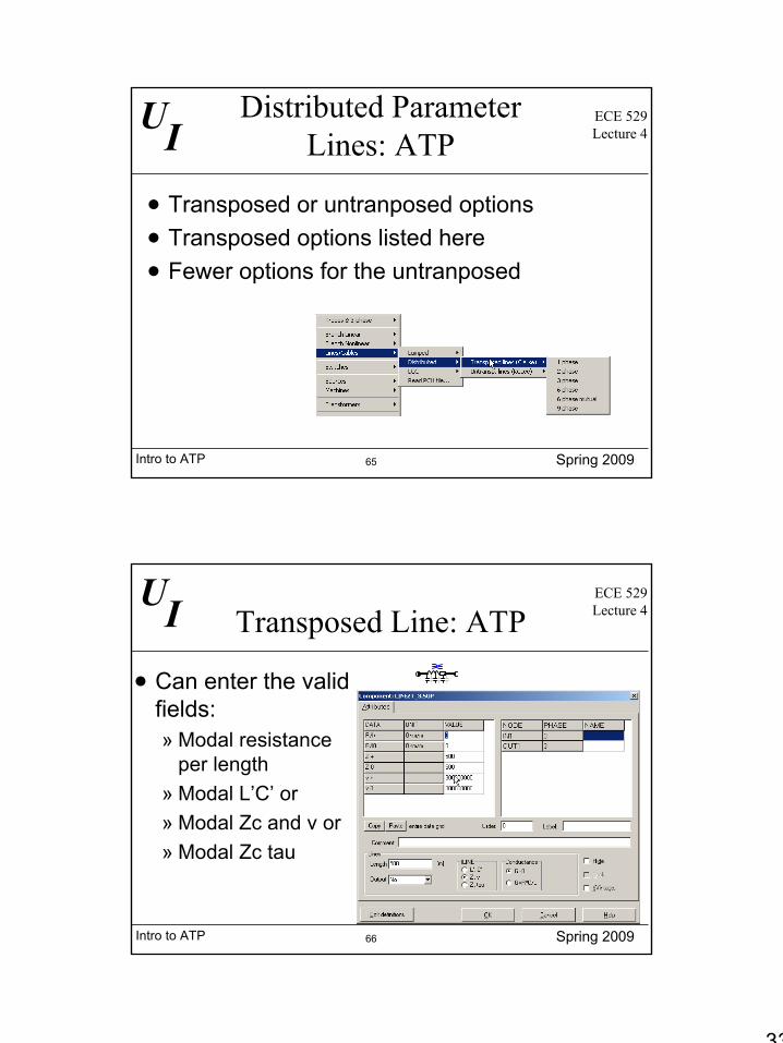
Distributed Parameter Lines: ATP

• Transposed or untranposed options• Transposed options listed here• Fewer options for the untranposed


UIECE 529Lecture 4

66

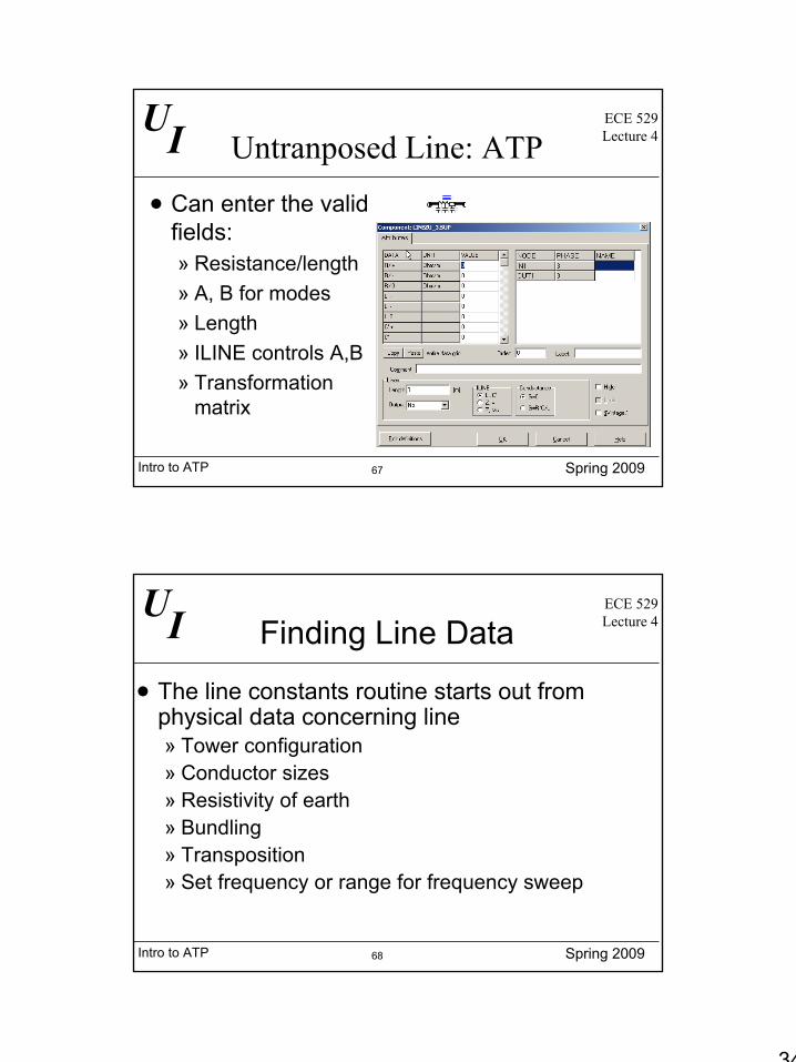
Transposed Line: ATP

• Can enter the valid fields: » Modal resistance

per length» Modal L’C’ or» Modal Zc and v or» Modal Zc tau

34


UIECE 529Lecture 4

67

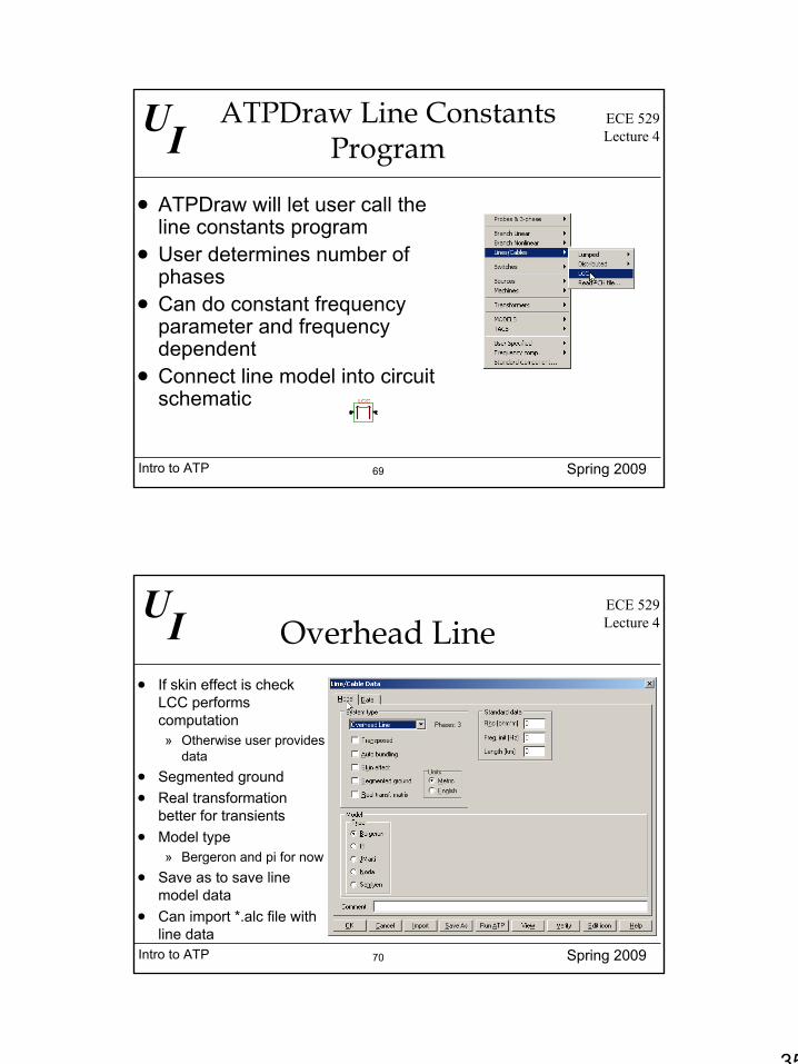
Untranposed Line: ATP

• Can enter the valid fields: » Resistance/length» A, B for modes» Length» ILINE controls A,B» Transformation

matrix


UIECE 529Lecture 4

68

Finding Line Data

• The line constants routine starts out from physical data concerning line» Tower configuration» Conductor sizes» Resistivity of earth» Bundling» Transposition» Set frequency or range for frequency sweep

35


UIECE 529Lecture 4

69

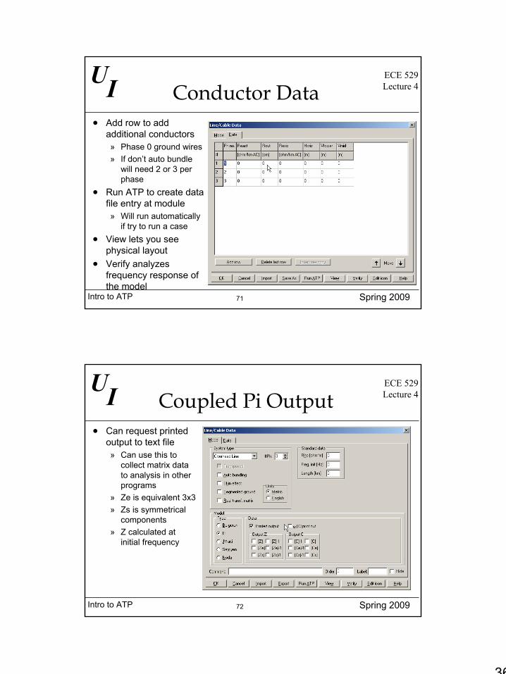
ATPDraw Line Constants Program

• ATPDraw will let user call the line constants program

• User determines number of phases

• Can do constant frequency parameter and frequency dependent

• Connect line model into circuit schematic LCC


UIECE 529Lecture 4

70

Overhead Line• If skin effect is check

LCC performs computation» Otherwise user provides

data• Segmented ground• Real transformation

better for transients• Model type

» Bergeron and pi for now• Save as to save line

model data• Can import *.alc file with

line data

36


UIECE 529Lecture 4

71

Conductor Data• Add row to add

additional conductors» Phase 0 ground wires» If don’t auto bundle

will need 2 or 3 per phase

• Run ATP to create data file entry at module» Will run automatically

if try to run a case• View lets you see

physical layout• Verify analyzes

frequency response of the model


UIECE 529Lecture 4

72

Coupled Pi Output• Can request printed

output to text file» Can use this to

collect matrix data to analysis in other programs

» Ze is equivalent 3x3» Zs is symmetrical

components» Z calculated at

initial frequency

37


UIECE 529Lecture 4

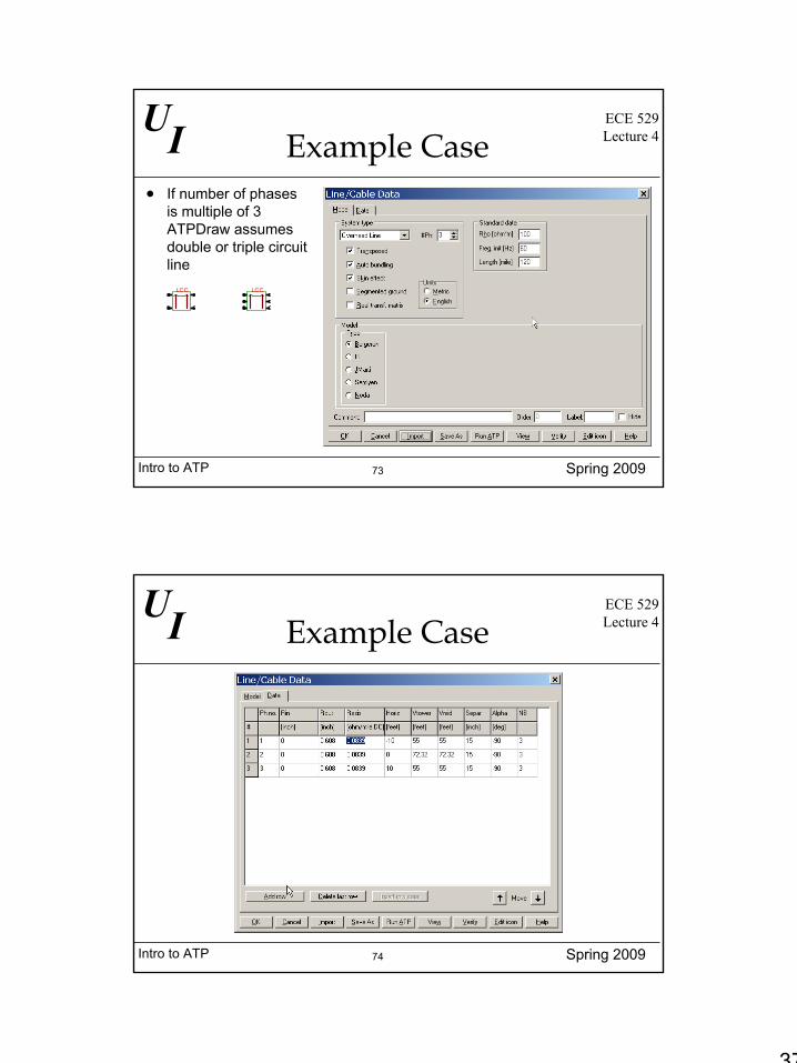
73

Example Case• If number of phases

is multiple of 3 ATPDraw assumes double or triple circuit line

LCC LCC


UIECE 529Lecture 4

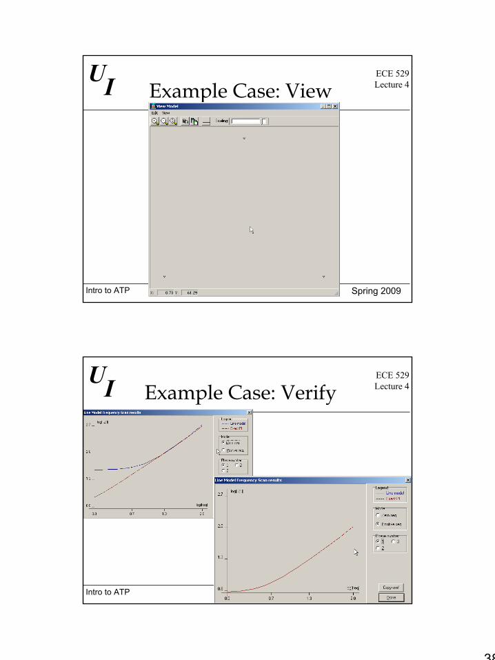
74

Example Case

38


UIECE 529Lecture 4

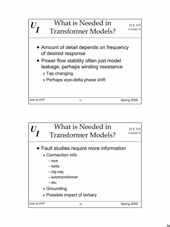
75

Example Case: View


UIECE 529Lecture 4

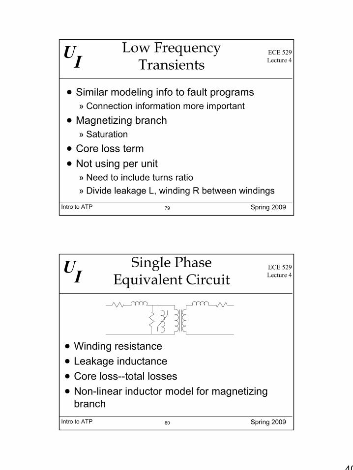
76

Example Case: Verify

39


UIECE 529Lecture 4

77

What is Needed in Transformer Models?

• Amount of detail depends on frequency of desired response

• Power flow stability often just model leakage, perhaps winding resistance» Tap changing» Perhaps wye-delta phase shift


UIECE 529Lecture 4

78

What is Needed in Transformer Models?

• Fault studies require more information» Connection info

– wye– delta– zig-zag– autotransformer– etc.

» Grounding» Possible impact of tertiary

40


UIECE 529Lecture 4

79

Low Frequency Transients

• Similar modeling info to fault programs» Connection information more important

• Magnetizing branch» Saturation

• Core loss term• Not using per unit

» Need to include turns ratio» Divide leakage L, winding R between windings


UIECE 529Lecture 4

80

Single Phase Equivalent Circuit

• Winding resistance• Leakage inductance• Core loss--total losses• Non-linear inductor model for magnetizing

branch

41


UIECE 529Lecture 4

81

ATP Options

• Ideal transformer component• Saturable transformer component• BCTran -- preprocessor that converts

description of transformer to coupled RL• Can also create manually using coupled RL

branches


UIECE 529Lecture 4

82

Ideal transformer component

• Combines ideal transformer with ideal source » Simply enter transformation ratio » Can be used to implement floating source too» Uses frequency from basic ATPDraw settings

– Need to make sure this matches system frequency– Setting “Branch = 0” forces ATP to use this

frequency– “Branch = 1” can avoid this (Vm=1E-20)

42


UIECE 529Lecture 4

83

Accessing Transformer Models

• Note that three phase and single phase options


UIECE 529Lecture 4

84

Dialog box

43


UIECE 529Lecture 4

85

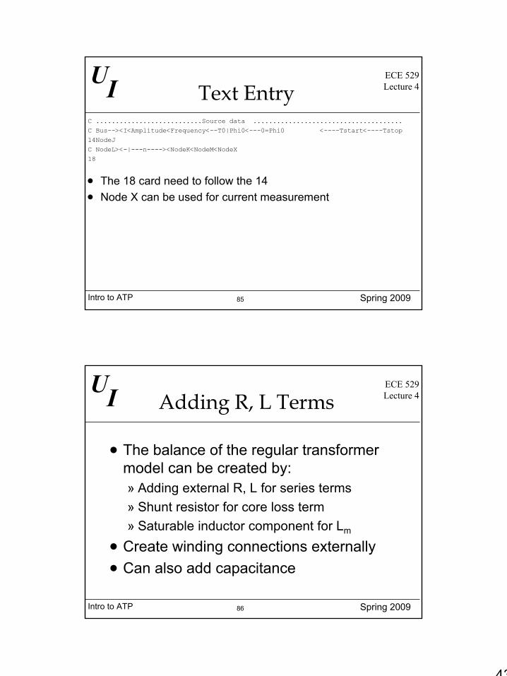
Text EntryC ...........................Source data ......................................C Bus--><I<Amplitude<Frequency<--T0|Phi0<---0=Phi0 <----Tstart<----Tstop14NodeJC NodeL><-|---n----><NodeK<NodeM<NodeX18

• The 18 card need to follow the 14• Node X can be used for current measurement


UIECE 529Lecture 4

86

Adding R, L Terms

• The balance of the regular transformer model can be created by:» Adding external R, L for series terms» Shunt resistor for core loss term» Saturable inductor component for Lm

• Create winding connections externally• Can also add capacitance

44


UIECE 529Lecture 4

87

Limitations

• Limited to two winding transformers• It is very easy to create numerical

problems in the simulation with the ideal transformer


UIECE 529Lecture 4

88

Saturable Transformer

• Model has built-in circuit elements» Winding resistance» Leakage inductance (can’t enter 0)» Core loss resistance» Magnetizing branch

– not entered as an L in mH» Can set all except leakage to 0 to simplify» Enter winding to winding ratios

45


UIECE 529Lecture 4

89

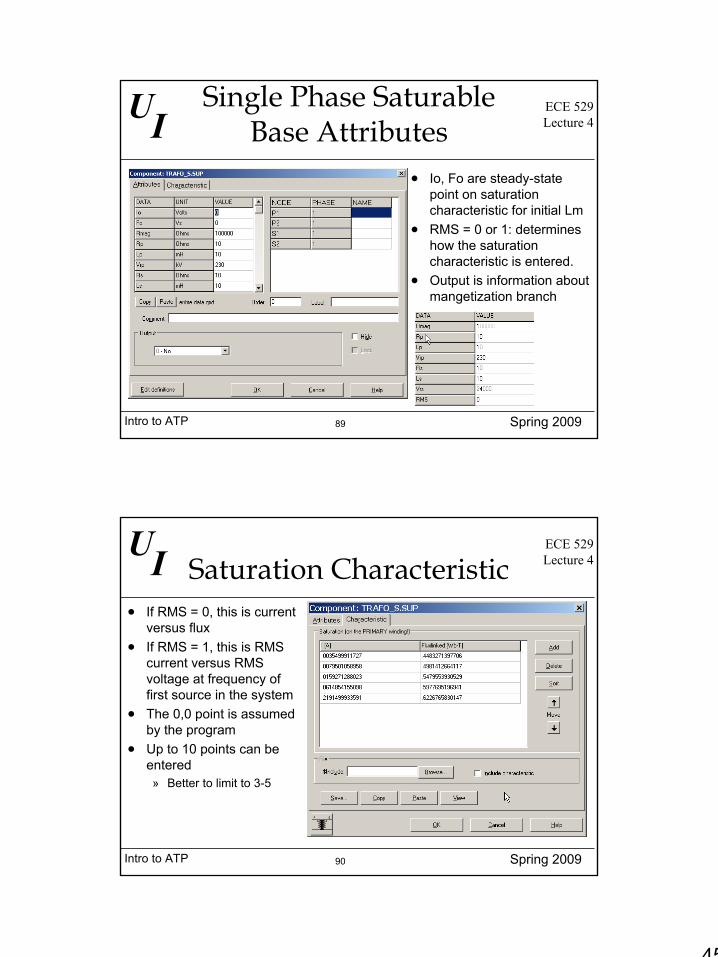
Single Phase SaturableBase Attributes

• Io, Fo are steady-state point on saturation characteristic for initial Lm

• RMS = 0 or 1: determines how the saturation characteristic is entered.

• Output is information about mangetization branch


UIECE 529Lecture 4

90

Saturation Characteristic• If RMS = 0, this is current

versus flux• If RMS = 1, this is RMS

current versus RMS voltage at frequency of first source in the system

• The 0,0 point is assumed by the program

• Up to 10 points can be entered» Better to limit to 3-5

46


UIECE 529Lecture 4

91

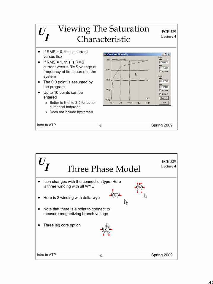
Viewing The Saturation Characteristic

• If RMS = 0, this is current versus flux

• If RMS = 1, this is RMS current versus RMS voltage at frequency of first source in the system

• The 0,0 point is assumed by the program

• Up to 10 points can be entered» Better to limit to 3-5 for better

numerical behavior» Does not include hysteresis


UIECE 529Lecture 4

92

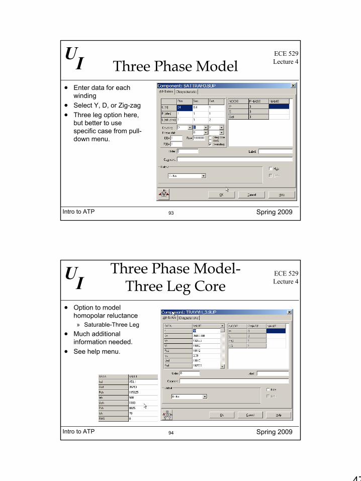
Three Phase Model• Icon changes with the connection type. Here

is three winding with all WYE

• Here is 2 winding with delta-wye

• Note that there is a point to connect to measure magnetizing branch voltage

• Three leg core option

47


UIECE 529Lecture 4

93

Three Phase Model• Enter data for each

winding• Select Y, D, or Zig-zag• Three leg option here,

but better to use specific case from pull-down menu.


UIECE 529Lecture 4

94

Three Phase Model-Three Leg Core

• Option to model homopolar reluctance» Saturable-Three Leg

• Much additional information needed.

• See help menu.

48


UIECE 529Lecture 4

95

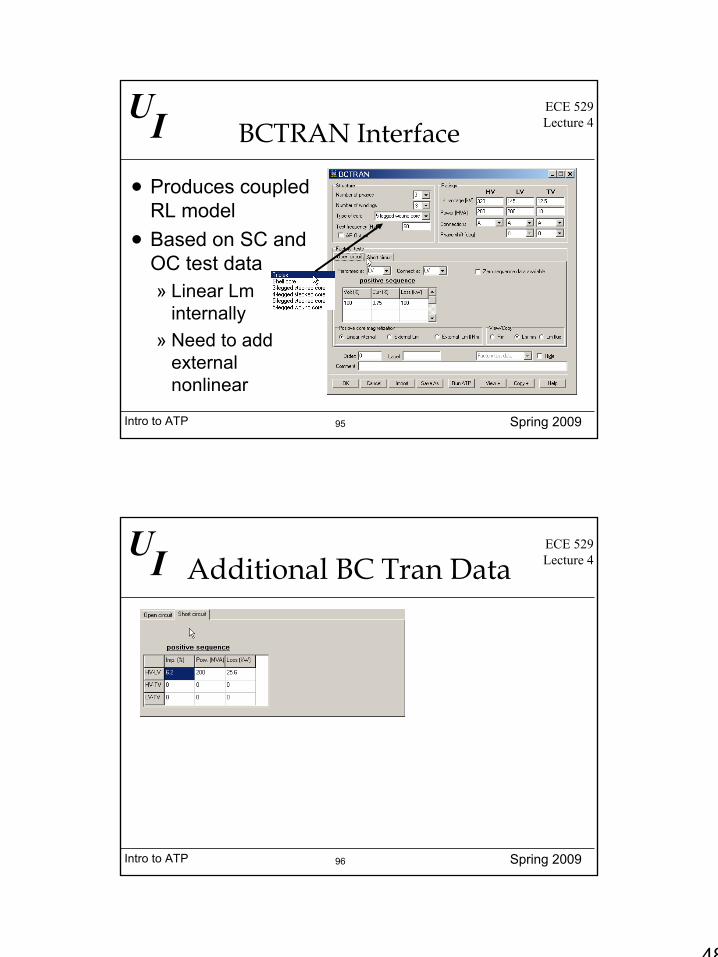
BCTRAN Interface

• Produces coupled RL model

• Based on SC and OC test data» Linear Lm

internally» Need to add

external nonlinear


UIECE 529Lecture 4

96

Additional BC Tran Data

49


UIECE 529Lecture 4

97

Nonlinear Devices• Models for resistors and

inductors» Differ model implementation

• The Type 98 and Type 93 inductors do not include hysteresis» Same user data as

saturation in saturable xfmr» Set with initial conditions


UIECE 529Lecture 4

98

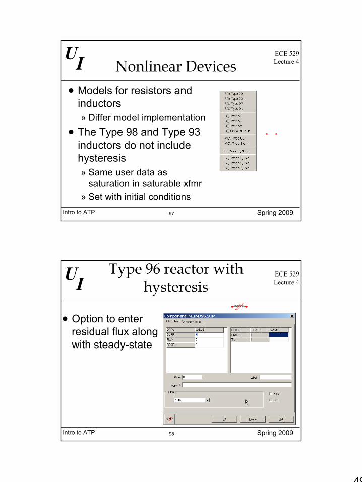
Type 96 reactor with hysteresis

• Option to enter residual flux along with steady-state

50


UIECE 529Lecture 4

99

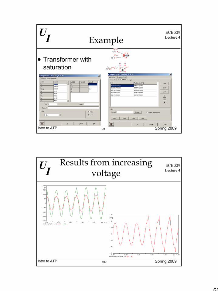
Example

• Transformer with saturation U SRC

SRC1

SRC2

B12

B13


UIECE 529Lecture 4

100

Results from increasing voltage

(f ile Exampl1.pl4; x-v ar t) v :B13 v :B12 0.00 0.02 0.04 0.06 0.08 0.10[s]

-200

-150

-100

-50

0

50

100

150

200[V]

(f ile Exampl1.pl4; x-v ar t) c :SRC -B12 0.00 0.02 0.04 0.06 0.08 0.10[s]

-6

-4

-2

0

2

4

6

[mA]

Documents

Lecture ATP