Embed Size (px)
Citation preview
Local eigenvalue statistics of random band matrices
Tatyana Shcherbinabased on the joint papers with M.Shcherbina
Princeton University
Analysis seminar, IAS, Feb 28, 2018
T. Shcherbina (PU) Local regime of RBM 02/28/2018 1 / 28
Local statistics, localization and delocalization
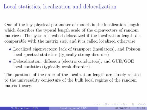
One of the key physical parameter of models is the localization length,which describes the typical length scale of the eigenvectors of randommatrices. The system is called delocalized if the localization length ` iscomparable with the matrix size, and it is called localized otherwise.
Localized eigenvectors: lack of transport (insulators), and Poissonlocal spectral statistics (typically strong disorder)Delocalization: diffusion (electric conductors), and GUE/GOElocal statistics (typically weak disorder).
The questions of the order of the localization length are closely relatedto the universality conjecture of the bulk local regime of the randommatrix theory.
T. Shcherbina (PU) Local regime of RBM 02/28/2018 2 / 28
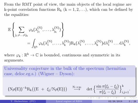
From the RMT point of view, the main objects of the local regime arek-point correlation functions Rk (k = 1, 2, . . .), which can be defined bythe equalities:
E
∑j1 6=... 6=jk
ϕk(λ(N)j1 , . . . , λ
(N)jk )
=
∫Rkϕk(λ
(N)1 , . . . , λ
(N)k )Rk(λ
(N)1 , . . . , λ
(N)k )dλ(N)
1 . . . dλ(N)k ,
where ϕk : Rk → C is bounded, continuous and symmetric in itsarguments.
Universality conjecture in the bulk of the spectrum (hermitiancase, deloc.eg.s.) (Wigner – Dyson):
(Nρ(E))−kRk({E + ξj/Nρ(E)}
) N→∞−→ det{sinπ(ξi − ξj)
π(ξi − ξj)
}k
i,j=1.
T. Shcherbina (PU) Local regime of RBM 02/28/2018 3 / 28
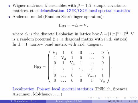
Wigner matrices, β-ensembles with β = 1, 2, sample covariancematrices, etc.: delocalization, GUE/GOE local spectral statisticsAnderson model (Random Schrodinger operators):
HRS = −4+ V,
where 4 is the discrete Laplacian in lattice box Λ = [1, n]d ∩ Zd, Vis a random potential (i.e. a diagonal matrix with i.i.d. entries).In d = 1: narrow band matrix with i.i.d. diagonal
HRS =
V1 1 0 0 . . . 01 V2 1 0 . . . 00 1 V3 1 . . . 0...
......
. . ....
...0 . . . 0 1 Vn−1 10 . . . 0 0 1 Vn
.
Localization, Poisson local spectral statistics (Frohlich, Spencer,Aizenman, Molchanov, . . . )
T. Shcherbina (PU) Local regime of RBM 02/28/2018 4 / 28
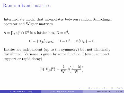
Random band matrices
Intermediate model that interpolates between random Schrodingeroperator and Wigner matrices.
Λ = [1, n]d ∩ Zd is a lattice box, N = nd.
H = {Hjk}j,k∈Λ, H = H∗, E{Hjk} = 0.
Entries are independent (up to the symmetry) but not identicallydistributed. Variance is given by some function J (even, compactsupport or rapid decay)
E{|Hjk|2} =1
Wd J( |j− k|
W
)
T. Shcherbina (PU) Local regime of RBM 02/28/2018 5 / 28
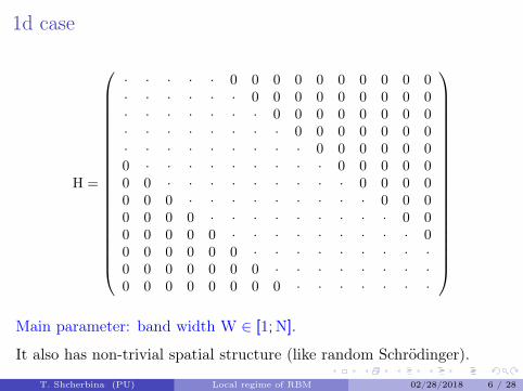
1d case
H =
· · · · · 0 0 0 0 0 0 0 0 0 0· · · · · · 0 0 0 0 0 0 0 0 0· · · · · · · 0 0 0 0 0 0 0 0· · · · · · · · 0 0 0 0 0 0 0· · · · · · · · · 0 0 0 0 0 00 · · · · · · · · · 0 0 0 0 00 0 · · · · · · · · · 0 0 0 00 0 0 · · · · · · · · · 0 0 00 0 0 0 · · · · · · · · · 0 00 0 0 0 0 · · · · · · · · · 00 0 0 0 0 0 · · · · · · · · ·0 0 0 0 0 0 0 · · · · · · · ·0 0 0 0 0 0 0 0 · · · · · · ·
Main parameter: band width W ∈ [1;N].
It also has non-trivial spatial structure (like random Schrodinger).
T. Shcherbina (PU) Local regime of RBM 02/28/2018 6 / 28
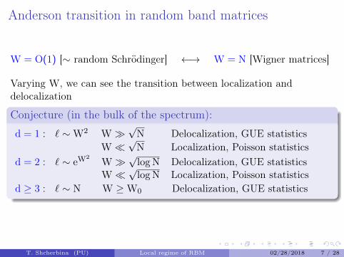
Anderson transition in random band matrices
W = O(1) [∼ random Schrodinger] ←→ W = N [Wigner matrices]
Varying W, we can see the transition between localization anddelocalization
Conjecture (in the bulk of the spectrum):
d = 1 : ` ∼W2 W�√N Delocalization, GUE statistics
W�√N Localization, Poisson statistics
d = 2 : ` ∼ eW2 W�√log N Delocalization, GUE statistics
W�√log N Localization, Poisson statistics
d ≥ 3 : ` ∼ N W ≥W0 Delocalization, GUE statistics
T. Shcherbina (PU) Local regime of RBM 02/28/2018 7 / 28
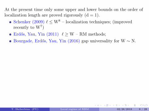
At the present time only some upper and lower bounds on the order oflocalization length are proved rigorously (d = 1).
Schenker (2009) ` ≤W8 – localization techniques; (improvedrecently to W7)Erdos, Yau, Yin (2011) ` ≥W – RM methods;Bourgade, Erdos, Yau, Yin (2016) gap universality for W ∼ N.
Main problem: to control the resolvent G(z) = (H− z)−1 forε := Im z ∼ 1/N (more precisely, to obtain the bounds forE{|G(E + iε)|2}). The techniques allows to obtain the control only forε ∼ 1/W. Such control can give a bounds for the localization length,but only in a weak sense, i.e. the estimates hold for “most”eigenfunctions only:
Erdos, Knowles (2011): `�W7/6;Erdos, Knowles, Yau, Yin (2012): `�W5/4 (not uniform in N).
T. Shcherbina (PU) Local regime of RBM 02/28/2018 8 / 28
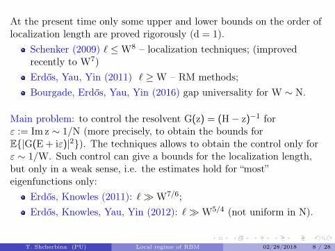
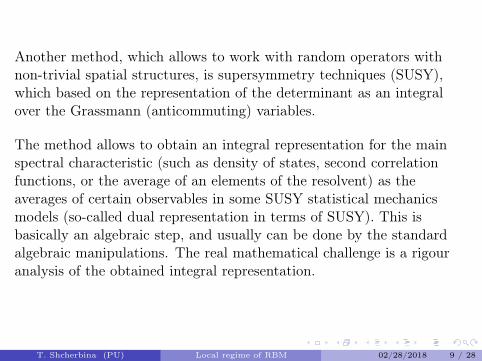
Another method, which allows to work with random operators withnon-trivial spatial structures, is supersymmetry techniques (SUSY),which based on the representation of the determinant as an integralover the Grassmann (anticommuting) variables.
The method allows to obtain an integral representation for the mainspectral characteristic (such as density of states, second correlationfunctions, or the average of an elements of the resolvent) as theaverages of certain observables in some SUSY statistical mechanicsmodels (so-called dual representation in terms of SUSY). This isbasically an algebraic step, and usually can be done by the standardalgebraic manipulations. The real mathematical challenge is a rigouranalysis of the obtained integral representation.
T. Shcherbina (PU) Local regime of RBM 02/28/2018 9 / 28
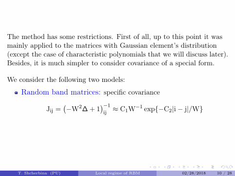
The method has some restrictions. First of all, up to this point it wasmainly applied to the matrices with Gaussian element’s distribution(except the case of characteristic polynomials that we will discuss later).Besides, it is much simpler to consider covariance of a special form.
We consider the following two models:
Random band matrices: specific covariance
Jij =(−W2∆ + 1
)−1ij ≈ C1W−1 exp{−C2|i− j|/W}
T. Shcherbina (PU) Local regime of RBM 02/28/2018 10 / 28
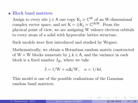
Block band matricesAssign to every site j ∈ Λ one copy Kj ' CW of an W-dimensionalcomplex vector space, and set K = ⊕Kj ' C|Λ|W. From thephysical point of view, we are assigning W valence electron orbitalsto every atom of a solid with hypercubic lattice structure.
Such models were first introduced and studied by Wegner.
Mathematically, we obtain a Hermitian random matrix constructedof W ×W blocks numerate by j, k ∈ Λ, and the variance in eachblock is a fixed number Jjk, where we take
J = 1/W + α∆/W, α < 1/4d.
This model is one of the possible realizations of the Gaussianrandom band matrices.
T. Shcherbina (PU) Local regime of RBM 02/28/2018 11 / 28
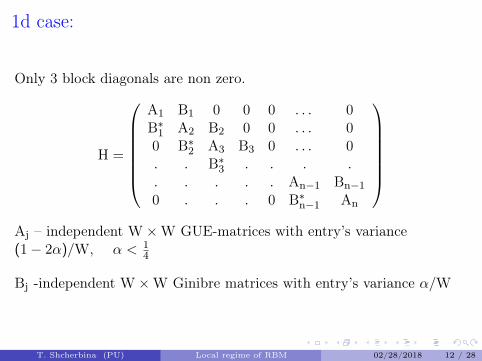
1d case:
Only 3 block diagonals are non zero.
H =
A1 B1 0 0 0 . . . 0B∗1 A2 B2 0 0 . . . 00 B∗2 A3 B3 0 . . . 0. . B∗3 . . . .. . . . . An−1 Bn−10 . . . 0 B∗n−1 An
Aj – independent W ×W GUE-matrices with entry’s variance(1− 2α)/W, α < 1
4
Bj -independent W ×W Ginibre matrices with entry’s variance α/W
T. Shcherbina (PU) Local regime of RBM 02/28/2018 12 / 28
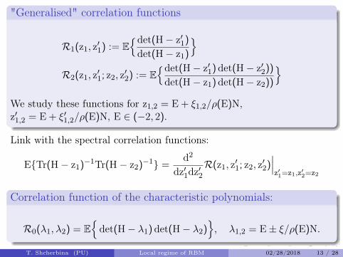
"Generalised" correlation functions
R1(z1, z′1) := E{det(H− z′1)
det(H− z1)
}R2(z1, z′1; z2, z′2) := E
{det(H− z′1) det(H− z′2))
det(H− z1) det(H− z2))
}We study these functions for z1,2 = E + ξ1,2/ρ(E)N,z′1,2 = E + ξ′1,2/ρ(E)N, E ∈ (−2, 2).
Link with the spectral correlation functions:
E{Tr(H− z1)−1Tr(H− z2)−1} =d2
dz′1dz′2R(z1, z′1; z2, z′2)
∣∣∣z′1=z1,z′2=z2
Correlation function of the characteristic polynomials:
R0(λ1, λ2) = E{det(H− λ1) det(H− λ2)
}, λ1,2 = E± ξ/ρ(E)N.
T. Shcherbina (PU) Local regime of RBM 02/28/2018 13 / 28
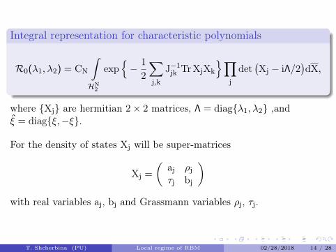
Integral representation for characteristic polynomials
R0(λ1, λ2) = CN
∫HN
2
exp{− 1
2
∑j,k
J−1jk TrXjXk
}∏j
det(Xj − iΛ/2
)dX,
where {Xj} are hermitian 2× 2 matrices, Λ = diag{λ1, λ2} ,andξ = diag{ξ,−ξ}.
For the density of states Xj will be super-matrices
Xj =
(aj ρjτj bj
)with real variables aj, bj and Grassmann variables ρj, τj.
T. Shcherbina (PU) Local regime of RBM 02/28/2018 14 / 28
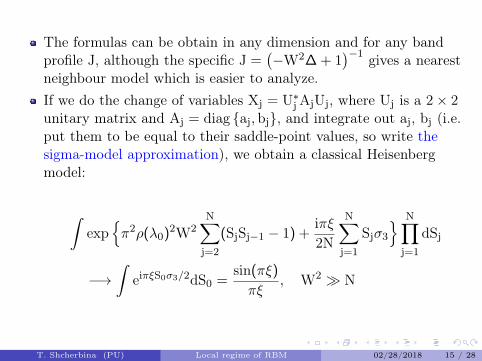
The formulas can be obtain in any dimension and for any bandprofile J, although the specific J =
(−W2∆ + 1
)−1 gives a nearestneighbour model which is easier to analyze.If we do the change of variables Xj = U∗j AjUj, where Uj is a 2× 2unitary matrix and Aj = diag {aj, bj}, and integrate out aj, bj (i.e.put them to be equal to their saddle-point values, so write thesigma-model approximation), we obtain a classical Heisenbergmodel:
∫exp
{π2ρ(λ0)2W2
N∑j=2
(SjSj−1 − 1) +iπξ2N
N∑j=1
Sjσ3
} N∏j=1
dSj
−→∫
eiπξS0σ3/2dS0 =sin(πξ)
πξ, W2 � N
T. Shcherbina (PU) Local regime of RBM 02/28/2018 15 / 28
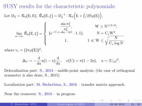
SUSY results for the characteristic polynomials:
Let D2 = R0(E,E), R0(E, ξ) = D−12 · R0
(E + ξ/2Nρ(E)
).
limn→∞
R0(E, ξ) =
sinπξπξ
, W ≥ N1/2+θ;
(e−C∗t∗∆U−iξν · 1, 1), N = C∗W2
1, 1�W ≤√
NC∗ log N
,
where t∗ = (2πρ(E))2,
∆U = − ddx
x(1− x)ddx, ν(U) = π(1− 2x), x = |U12|2.
Delocalization part: S., 2013 – saddle-point analysis; (the case of orthogonalsymmetry is also done, S., 2015)
Localization part: M. Shcherbina, S., 2016 – transfer matrix approach.
Near the crossover: S., 2018 – in progress
T. Shcherbina (PU) Local regime of RBM 02/28/2018 16 / 28
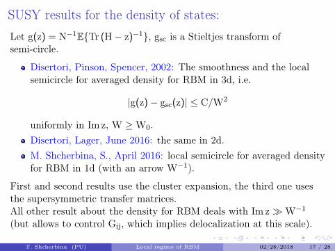
SUSY results for the density of states:Let g(z) = N−1E{Tr (H− z)−1}, gsc is a Stieltjes transform ofsemi-circle.
Disertori, Pinson, Spencer, 2002: The smoothness and the localsemicircle for averaged density for RBM in 3d, i.e.
|g(z)− gsc(z)| ≤ C/W2
uniformly in Im z, W ≥W0.Disertori, Lager, June 2016: the same in 2d.M. Shcherbina, S., April 2016: local semicircle for averaged densityfor RBM in 1d (with an arrow W−1).
First and second results use the cluster expansion, the third one usesthe supersymmetric transfer matrices.All other result about the density for RBM deals with Im z�W−1
(but allows to control Gij, which implies delocalization at this scale).
T. Shcherbina (PU) Local regime of RBM 02/28/2018 17 / 28
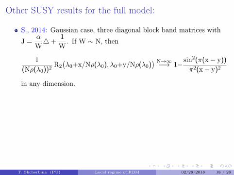
Other SUSY results for the full model:
S., 2014: Gaussian case, three diagonal block band matrices with
J =α
W4+
1W
. If W ∼ N, then
1(Nρ(λ0))2 R2
(λ0+x/Nρ(λ0), λ0+y/Nρ(λ0)
) N→∞−→ 1−sin2(π(x− y))
π2(x− y)2
in any dimension.
Erdos, Bao, 2015: Combining this techniques with Green’sfunction comparison strategy (Erdos-Yau), they proved
` ≥W7/6
in a strong sense for the block band matrices with more or lessgeneral element’s distribution (subexponential tails, four Gaussianmoments).
T. Shcherbina (PU) Local regime of RBM 02/28/2018 18 / 28
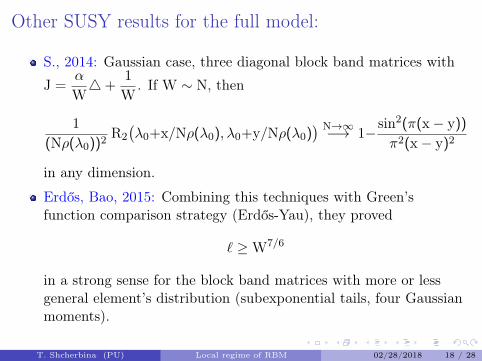
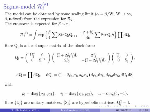
Sigma-model R(σ)2
The model can be obtained by some scaling limit (α = β/W, W→∞,β,n-fixed) from the expression for R2.The crossover is expected for β ∼ n.
R(σ)2 =
∫exp
{β4
∑StrQjQj+1 +
ε+ iξ4n
∑StrQjΛ
}∏dQj
Here Qj is a 4× 4 super matrix of the block form:
Qj =
(U∗j 00 S−1
j
)((I + 2ρjτj)L 2τj
2ρj −(I− 2ρjτj)L
)(Uj 00 Sj
),
dQ =∏
dQj, dQj = (1− 2ρj1τj1ρj2τj2) dρj1dτj1 dρj2dτj2 dUj dSj
with
ρj = diag{ρj1, ρj2}, τj = diag{τj1, ρj2}, L = diag{1,−1}.
Here {Uj} are unitary matrices, {Sj} are hyperbolic matrices, Q2j = I.
T. Shcherbina (PU) Local regime of RBM 02/28/2018 19 / 28
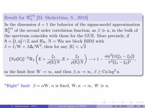
Result for R(σ)2 [M. Shcherbina, S., 2018]
In the dimension d = 1 the behavior of the sigma-model approximationR(σ)
2 of the second order correlation function, as β � n, in the bulk ofthe spectrum coincides with those for the GUE. More precisely, ifΛ = [1, n] ∩ Z and HN, N = Wn are block RBM withJ = 1/W + β∆/W2, then for any |E| <
√2
(Nρ(E))−2R2
(E +
ξ1ρ(E)N
,E +ξ2
ρ(E)N
)−→ 1− sin2(π(ξ1 − ξ2))
π2(ξ1 − ξ2)2 ,
in the limit first W→∞, and then β, n→∞, β ≥ Cn log2 n.
"Right" limit: β = αW, α is fixed, W, n→∞, W� n.
T. Shcherbina (PU) Local regime of RBM 02/28/2018 20 / 28
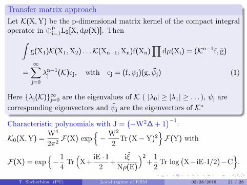
Transfer matrix approachLet K(X,Y) be the p-dimensional matrix kernel of the compact integraloperator in ⊕p
i=1L2[X, dµ(X)]. Then∫g(X1)K(X1,X2) . . .K(Xn−1,Xn)f(Xn)
∏dµ(Xi) = (Kn−1f, g)
=∞∑j=0
λn−1j (K)cj, with cj = (f, ψj)(g, ψj) (1)
Here {λj(K)}∞j=0 are the eigenvalues of K ( |λ0| ≥ |λ1| ≥ . . . ), ψj arecorresponding eigenvectors and ψj are the eigenvectors of K∗
Characteristic polynomials with J =(−W2∆ + 1
)−1:
K0(X,Y) =W4
2π2 F(X) exp{− W2
2Tr (X−Y)2
}F(Y) with
F(X) = exp{− 14Tr(X+
iE · I2
+iξ
Nρ(E)
)2+12Tr log
(X− iE ·I/2
)−C
}.
T. Shcherbina (PU) Local regime of RBM 02/28/2018 21 / 28
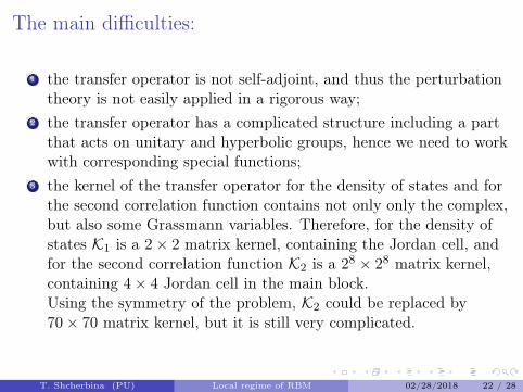
The main difficulties:
1 the transfer operator is not self-adjoint, and thus the perturbationtheory is not easily applied in a rigorous way;
2 the transfer operator has a complicated structure including a partthat acts on unitary and hyperbolic groups, hence we need to workwith corresponding special functions;
3 the kernel of the transfer operator for the density of states and forthe second correlation function contains not only only the complex,but also some Grassmann variables. Therefore, for the density ofstates K1 is a 2× 2 matrix kernel, containing the Jordan cell, andfor the second correlation function K2 is a 28 × 28 matrix kernel,containing 4× 4 Jordan cell in the main block.Using the symmetry of the problem, K2 could be replaced by70× 70 matrix kernel, but it is still very complicated.
T. Shcherbina (PU) Local regime of RBM 02/28/2018 22 / 28
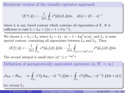
Resolvent version of the transfer operator approach
(Knf, g) = − 12πi
∮Lzn(G(z)f, g)dz, G(z) = (K − z)−1
where L is any closed contour which contains all eigenvalues of K. It issufficient to take L = L0 = {|z| = 1 + Cn−1},
We choose L = L1 ∪ L2 where L2 = {z : |z| = 1− log2 n/n}, and L1 is somespecial contour, containing all eigenvalues between L0 and L2. Then
(Knαf, g) = − 1
2πi
∮L1
zn(Gα(z)f, g)dz− 12πi
∮|z|=1−log2 n/n
zn(Gα(z)f, g)dz
The second integral is small since |z|n ≤ e− log2 n
Definition of asymptotically equivalent operators (n,W→∞)
AWn ∼ BWn ⇔∮
L1
zn((AWn− z)−1f, g)dz =
∮L1
zn((BWn− z)−1f, g)dz+ o(1)
for certain L1
T. Shcherbina (PU) Local regime of RBM 02/28/2018 23 / 28
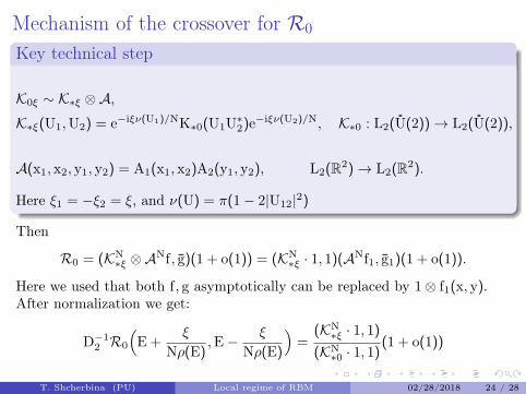
Mechanism of the crossover for R0
Key technical step
K0ξ ∼ K∗ξ ⊗A,K∗ξ(U1,U2) = e−iξν(U1)/NK∗0(U1U∗2)e−iξν(U2)/N, K∗0 : L2(U(2))→ L2(U(2)),
A(x1, x2, y1, y2) = A1(x1, x2)A2(y1, y2), L2(R2)→ L2(R2).
Here ξ1 = −ξ2 = ξ, and ν(U) = π(1− 2|U12|2)
Then
R0 = (KN∗ξ ⊗ANf, g)(1 + o(1)) = (KN
∗ξ · 1, 1)(ANf1, g1)(1 + o(1)).
Here we used that both f, g asymptotically can be replaced by 1⊗ f1(x, y).After normalization we get:
D−12 R0
(E +
ξ
Nρ(E),E− ξ
Nρ(E)
)=
(KN∗ξ · 1, 1)
(KN∗0 · 1, 1)
(1 + o(1))
T. Shcherbina (PU) Local regime of RBM 02/28/2018 24 / 28
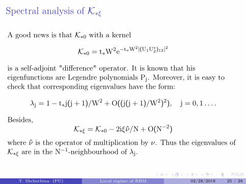
Spectral analysis of K∗ξ
A good news is that K∗0 with a kernel
K∗0 = t∗W2e−t∗W2|(U1U∗2)12|2
is a self-adjoint "difference" operator. It is known that hiseigenfunctions are Legendre polynomials Pj. Moreover, it is easy tocheck that corresponding eigenvalues have the form:
λj = 1− t∗j(j + 1)/W2 + O((j(j + 1)/W2)2), j = 0, 1 . . . .
Besides,K∗ξ = K∗0 − 2iξν/N + O(N−2)
where ν is the operator of multiplication by ν. Thus the eigenvalues ofK∗ξ are in the N−1-neighbourhood of λj.
T. Shcherbina (PU) Local regime of RBM 02/28/2018 25 / 28
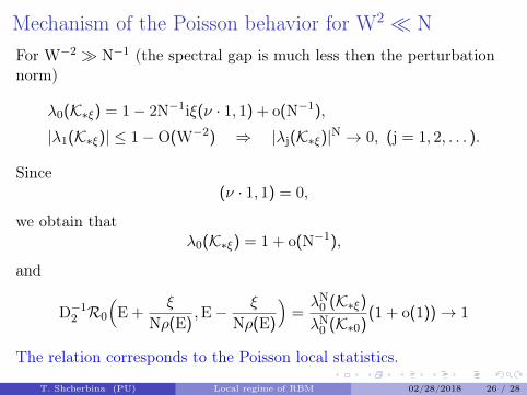
Mechanism of the Poisson behavior for W2 � NFor W−2 � N−1 (the spectral gap is much less then the perturbationnorm)
λ0(K∗ξ) = 1− 2N−1iξ(ν · 1, 1) + o(N−1),
|λ1(K∗ξ)| ≤ 1−O(W−2) ⇒ |λj(K∗ξ)|N → 0, (j = 1, 2, . . . ).
Since(ν · 1, 1) = 0,
we obtain thatλ0(K∗ξ) = 1 + o(N−1),
and
D−12 R0
(E +
ξ
Nρ(E),E− ξ
Nρ(E)
)=λN
0 (K∗ξ)λN
0 (K∗0)(1 + o(1))→ 1
The relation corresponds to the Poisson local statistics.
T. Shcherbina (PU) Local regime of RBM 02/28/2018 26 / 28
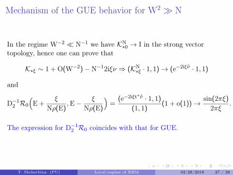
Mechanism of the GUE behavior for W2 � N
In the regime W−2 � N−1 we have KN∗0 → I in the strong vector
topology, hence one can prove that
K∗ξ ∼ 1 + O(W−2)−N−12iξν ⇒ (KN∗ξ · 1, 1)→ (e−2iξν · 1, 1)
and
D−12 R0
(E +
ξ
Nρ(E),E− ξ
Nρ(E)
)=
(e−2iξt∗ν · 1, 1)
(1, 1)(1 + o(1))→ sin(2πξ)
2πξ.
The expression for D−12 R0 coincides with that for GUE.
T. Shcherbina (PU) Local regime of RBM 02/28/2018 27 / 28
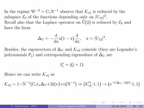
In the regime W−2 = C∗N−1 observe that K∗ξ is reduced by thesubspace E0 of the functions depending only on |U12|2.Recall also that the Laplace operator on U(2) is reduced by E0 andhave the form
∆U = − ddx
x(1− x)ddx, x = |U12|2.
Besides, the eigenvectors of ∆U and K∗0 coincide (they are Legendre’spolynomials Pj) and corresponding eigenvalues of ∆U are
λ∗j = j(j + 1).
Hence we can write K∗ξ as
K∗ξ ∼ 1−N−1(C∗t∗∆U+2iξν)+o(N−1)⇒ (KN∗ξ ·1, 1)→ (e−C∆U−2iξν ·1, 1)
T. Shcherbina (PU) Local regime of RBM 02/28/2018 28 / 28


![REAL EIGENVALUE ANALYSIS IN NASTRAN BY THE … · 2020. 8. 6. · Thedefinitions of the eigenvalue, the matrices [K] and [M], and their mathematical properties, dependon the type](https://img.pdfslide.net/doc/110x75/611001d3d01e0038fa00f89c/real-eigenvalue-analysis-in-nastran-by-the-2020-8-6-thedefinitions-of-the-eigenvalue.jpg)