50. Internationales Wissenschaftliches Kolloquium September, 19-23, 2005 Maschinenbau von Makro bis Nano /

Mechanical Engineering from Macro to Nano Proceedings Fakultät für Maschinenbau / Faculty of Mechanical Engineering

Startseite / Index: http://www.db-thueringen.de/servlets/DocumentServlet?id=15745

Impressum Herausgeber: Der Rektor der Technischen Universität llmenau Univ.-Prof. Dr. rer. nat. habil. Peter Scharff Redaktion: Referat Marketing und Studentische Angelegenheiten Andrea Schneider Fakultät für Maschinenbau

Univ.-Prof. Dr.-Ing. habil. Peter Kurtz, Univ.-Prof. Dipl.-Ing. Dr. med. (habil.) Hartmut Witte, Univ.-Prof. Dr.-Ing. habil. Gerhard Linß, Dr.-Ing. Beate Schlütter, Dipl.-Biol. Danja Voges, Dipl.-Ing. Jörg Mämpel, Dipl.-Ing. Susanne Töpfer, Dipl.-Ing. Silke Stauche

Redaktionsschluss: 31. August 2005 (CD-Rom-Ausgabe) Technische Realisierung: Institut für Medientechnik an der TU Ilmenau (CD-Rom-Ausgabe) Dipl.-Ing. Christian Weigel

Dipl.-Ing. Helge Drumm Dipl.-Ing. Marco Albrecht

Technische Realisierung: Universitätsbibliothek Ilmenau (Online-Ausgabe) Postfach 10 05 65 98684 Ilmenau

Verlag: Verlag ISLE, Betriebsstätte des ISLE e.V. Werner-von-Siemens-Str. 16 98693 llmenau © Technische Universität llmenau (Thür.) 2005 Diese Publikationen und alle in ihr enthaltenen Beiträge und Abbildungen sind urheberrechtlich geschützt. ISBN (Druckausgabe): 3-932633-98-9 (978-3-932633-98-0) ISBN (CD-Rom-Ausgabe): 3-932633-99-7 (978-3-932633-99-7) Startseite / Index: http://www.db-thueringen.de/servlets/DocumentServlet?id=15745

50. Internationales Wissenschaftliches Kolloquium Technische Universität Ilmenau

19.-23. September 2005 M. Oppermann / W. Sauer Cost Efficient Quality Strategies for Electronics Production

ABSTRACT In the last years the authors developed new and powerful quality cost models to optimize quality strategies in electronics production. These models are successful in use and were published in some books (see [1], [4] and [5]), tutorials, articles (see [2] and [3]) and presentations at important conferences like IWK99, ECTC2001, ISSE2002 and SMT HYBRID PACKAGING 2002, 2003 and 2004. These models look for the quality processes only to find out the optimized quality strategy by the minimum of costs. The next step was the development of an extension of these models to include the production process and its quality dependent properties into the cost models. The question is: How influences the improvement of a production process by investment the quality and the costs of the products? How much time does it need to reach a better quality level by lower costs? The new extension of the quality cost models gives help to the production engineers to make a decision about the right quality strategy. The basic quality cost model and the influence of investment will be explained in our presentation.

1. INTRODUCTION Controlled technological processes are the most important way to reach a high quality level in

mechanical engineering industries. Statistical Process Control (SPC) and Failure Mode Effect

Analysis (FMEA) are other ways to reach this goal. It is possible to use these methods also in

electronics production in the case of producing batches with a high number of same PCBs. But in a

production process with many different products and small batch sizes, there are relative high defect

rates and some technological processes may be uncontrolled. The objective of this publication is to

show new models to decrease the quality costs of such technological processes. A special part of

this publication describes the influence of investment to decrease the defect rate and so the

summary costs of an electronic product.

2. CHANGING THE QUALITY STRATEGY – THE BASIC QUALITY COST MODEL

Starting point of this paper is a chain of technological processes - for instance a SMT production

line as in Fig. 1. The SMT line consists of a PCB transport system, a solder paste printer, a chip

shooter, a pick-and-place machine, a reflow oven and an inspection system at the end. In this

example the process of solder paste printing is not well controlled and so there are some poorly

printed PCBs. These PCBs are represented by the defect rate p. What is the right way to fix this

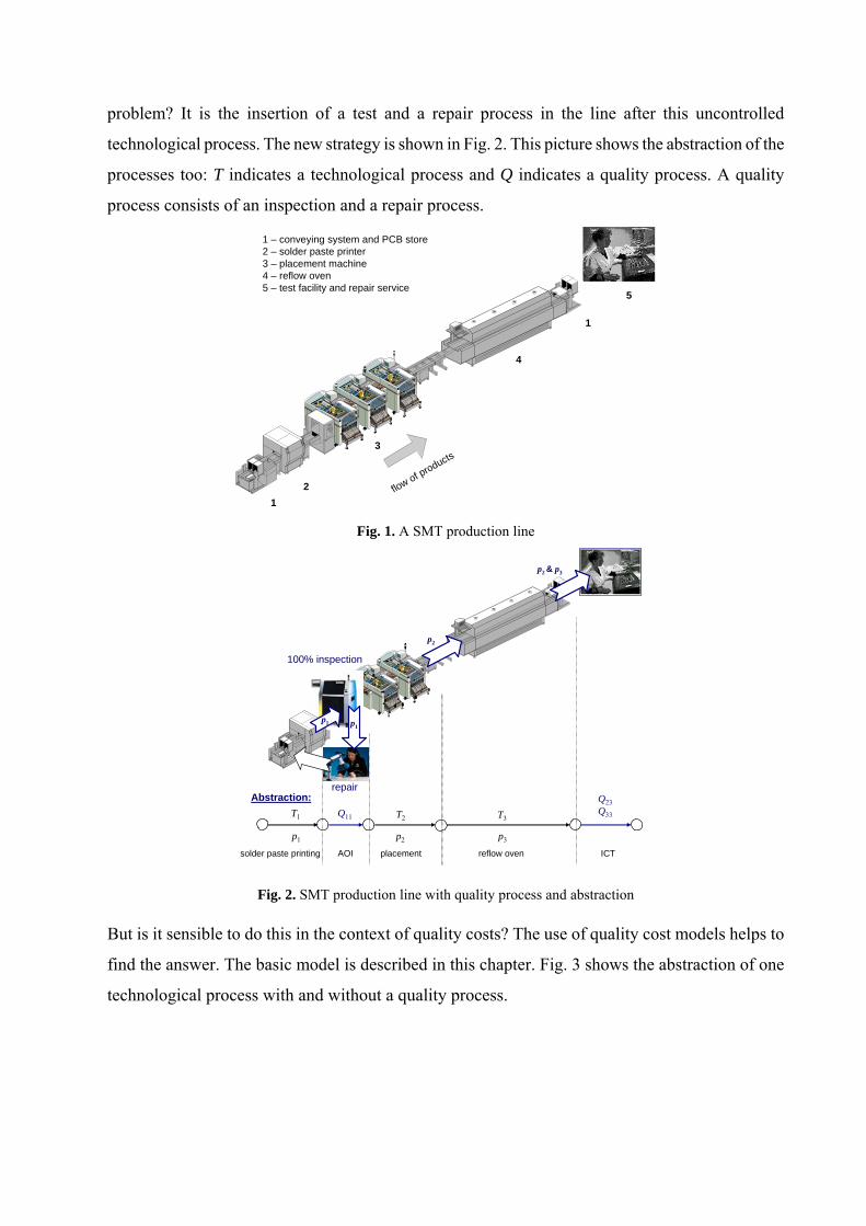
problem? It is the insertion of a test and a repair process in the line after this uncontrolled

technological process. The new strategy is shown in Fig. 2. This picture shows the abstraction of the

processes too: T indicates a technological process and Q indicates a quality process. A quality

process consists of an inspection and a repair process.

1

1

2

3

4

5

1 – conveying system and PCB store2 – solder paste printer3 – placement machine4 – reflow oven5 – test facility and repair service

flow of products

Fig. 1. A SMT production line

T1 Q11

p1

p1p1

100% inspection

Abstraction:repair

T2

p2

T3

p3

Q23Q33

p2

p2 & p3

solder paste printing AOI placement reflow oven ICT

Fig. 2. SMT production line with quality process and abstraction

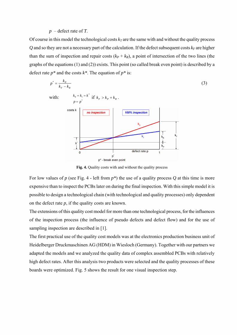
But is it sensible to do this in the context of quality costs? The use of quality cost models helps to

find the answer. The basic model is described in this chapter. Fig. 3 shows the abstraction of one

technological process with and without a quality process.

Fig. 3. Model for one technological process

The technological process T (see Fig. 3) has a defect rate p. In the first case a quality process Q

(consisting of the inspection process P with 100% inspection of the PCBs and the repair process R)

is added to detect and to eliminate these defects. The inspection and repair processes cause quality

costs. In the second case there is no quality process to detect and to remove the defects after the

technological process. But there is also a defect rate p ≠ 0 and the defects will be processed. It

means, the defects also cause quality costs, but later in the technological line (latest in the final

inspection process). With the view to these quality costs it is possible to define a virtual process

called defect subsequent process F. Now it is possible to answer the question: Which case is

cheaper – with or without a quality process right after the technological process? To answer this

question the following assumptions are necessary: All of the produced PCBs are inspected (100%

test), all PCBs with defects are identified and repaired, after the last technological process in the

line is a 100% test of the PCBs installed (for example an in-circuit test) and the quality costs are

calculated as costs per unit (for example per PCB).

To describe the quality costs of the above discussed two cases the following equations are used:

• Costs without an inspection after T:

FT kpkk ⋅+=0 (1)

• Costs with an inspection after T:

RPT kpkkk ⋅++=1 (2)

with:

kT – costs of the technological process T per unit

kF – defect subsequent costs per unit

kP – inspection costs per unit

kR – repair costs per unit

p – defect rate of T.

Of course in this model the technological costs kT are the same with and without the quality process

Q and so they are not a necessary part of the calculation. If the defect subsequent costs kF are higher

than the sum of inspection and repair costs (kP + kR), a point of intersection of the two lines (the

graphs of the equations (1) and (2)) exists. This point (so called break even point) is described by a

defect rate p* and the costs k*. The equation of p* is:

RF

P

kkkp−

=* (3)

with: if *

*10

pp

kkk

=

==RPF kkk +> .

Fig. 4. Quality costs with and without the quality process

For low values of p (see Fig. 4 - left from p*) the use of a quality process Q at this time is more

expensive than to inspect the PCBs later on during the final inspection. With this simple model it is

possible to design a technological chain (with technological and quality processes) only dependent

on the defect rate p, if the quality costs are known.

The extensions of this quality cost model for more than one technological process, for the influences

of the inspection process (the influence of pseudo defects and defect flow) and for the use of

sampling inspection are described in [1].

The first practical use of the quality cost models was at the electronics production business unit of

Heidelberger Druckmaschinen AG (HDM) in Wiesloch (Germany). Together with our partners we

adapted the models and we analyzed the quality data of complex assembled PCBs with relatively

high defect rates. After this analysis two products were selected and the quality processes of these

boards were optimized. Fig. 5 shows the result for one visual inspection step.

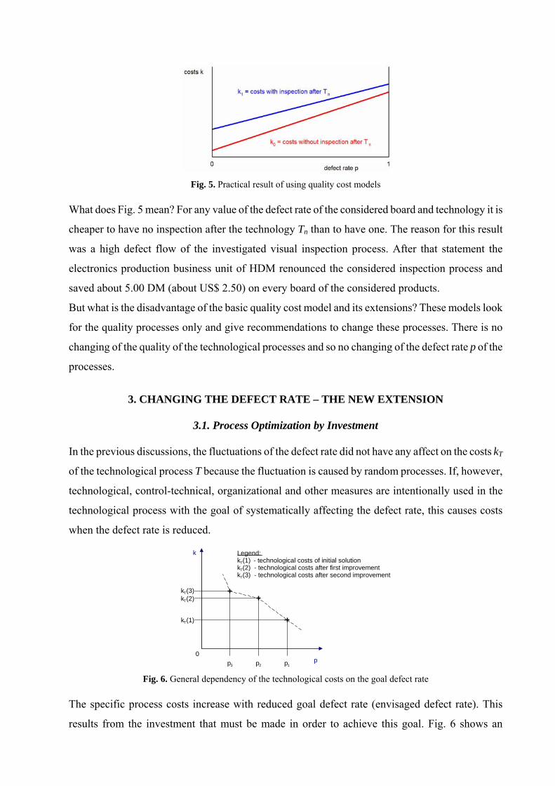
Fig. 5. Practical result of using quality cost models

What does Fig. 5 mean? For any value of the defect rate of the considered board and technology it is

cheaper to have no inspection after the technology Tn than to have one. The reason for this result

was a high defect flow of the investigated visual inspection process. After that statement the

electronics production business unit of HDM renounced the considered inspection process and

saved about 5.00 DM (about US$ 2.50) on every board of the considered products.

But what is the disadvantage of the basic quality cost model and its extensions? These models look

for the quality processes only and give recommendations to change these processes. There is no

changing of the quality of the technological processes and so no changing of the defect rate p of the

processes.

3. CHANGING THE DEFECT RATE – THE NEW EXTENSION

3.1. Process Optimization by Investment

In the previous discussions, the fluctuations of the defect rate did not have any affect on the costs kT

of the technological process T because the fluctuation is caused by random processes. If, however,

technological, control-technical, organizational and other measures are intentionally used in the

technological process with the goal of systematically affecting the defect rate, this causes costs

when the defect rate is reduced.

k

p

k T (2)

k T (1)

k T (3)

p2p3 p1

0

Legend:kT(1) - technological costs of initial solutionkT(2) - technological costs after first improvementkT(3) - technological costs after second improvement

Fig. 6. General dependency of the technological costs on the goal defect rate The specific process costs increase with reduced goal defect rate (envisaged defect rate). This

results from the investment that must be made in order to achieve this goal. Fig. 6 shows an

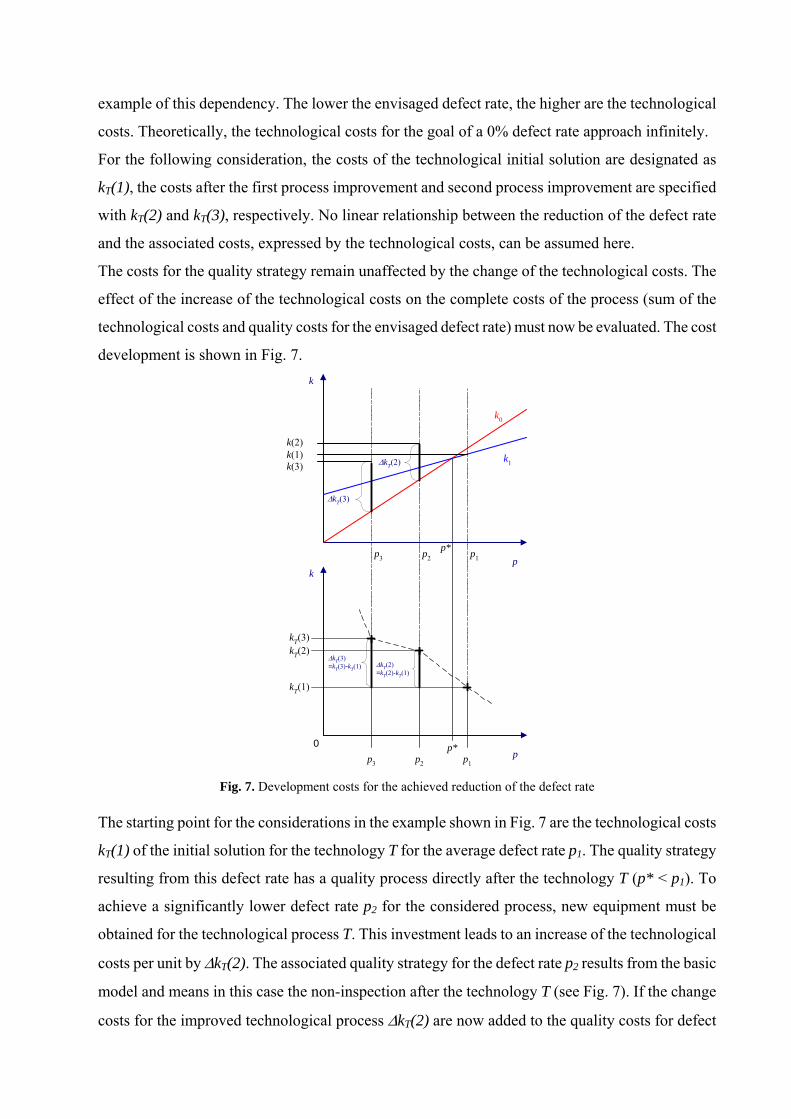
example of this dependency. The lower the envisaged defect rate, the higher are the technological

costs. Theoretically, the technological costs for the goal of a 0% defect rate approach infinitely.

For the following consideration, the costs of the technological initial solution are designated as

kT(1), the costs after the first process improvement and second process improvement are specified

with kT(2) and kT(3), respectively. No linear relationship between the reduction of the defect rate

and the associated costs, expressed by the technological costs, can be assumed here.

The costs for the quality strategy remain unaffected by the change of the technological costs. The

effect of the increase of the technological costs on the complete costs of the process (sum of the

technological costs and quality costs for the envisaged defect rate) must now be evaluated. The cost

development is shown in Fig. 7.

k

p

kT(2)

kT(1)

kT(3)

p2p3 p1

0

k

p

k(1)

ΔkT(2)=kT(2)-kT(1)

ΔkT(3)=kT(3)-kT(1)

ΔkT(3)

ΔkT(2)k(3)

k(2)

k0

k1

p*

p2p3 p1p*

Fig. 7. Development costs for the achieved reduction of the defect rate

The starting point for the considerations in the example shown in Fig. 7 are the technological costs

kT(1) of the initial solution for the technology T for the average defect rate p1. The quality strategy

resulting from this defect rate has a quality process directly after the technology T (p* < p1). To

achieve a significantly lower defect rate p2 for the considered process, new equipment must be

obtained for the technological process T. This investment leads to an increase of the technological

costs per unit by ΔkT(2). The associated quality strategy for the defect rate p2 results from the basic

model and means in this case the non-inspection after the technology T (see Fig. 7). If the change

costs for the improved technological process ΔkT(2) are now added to the quality costs for defect

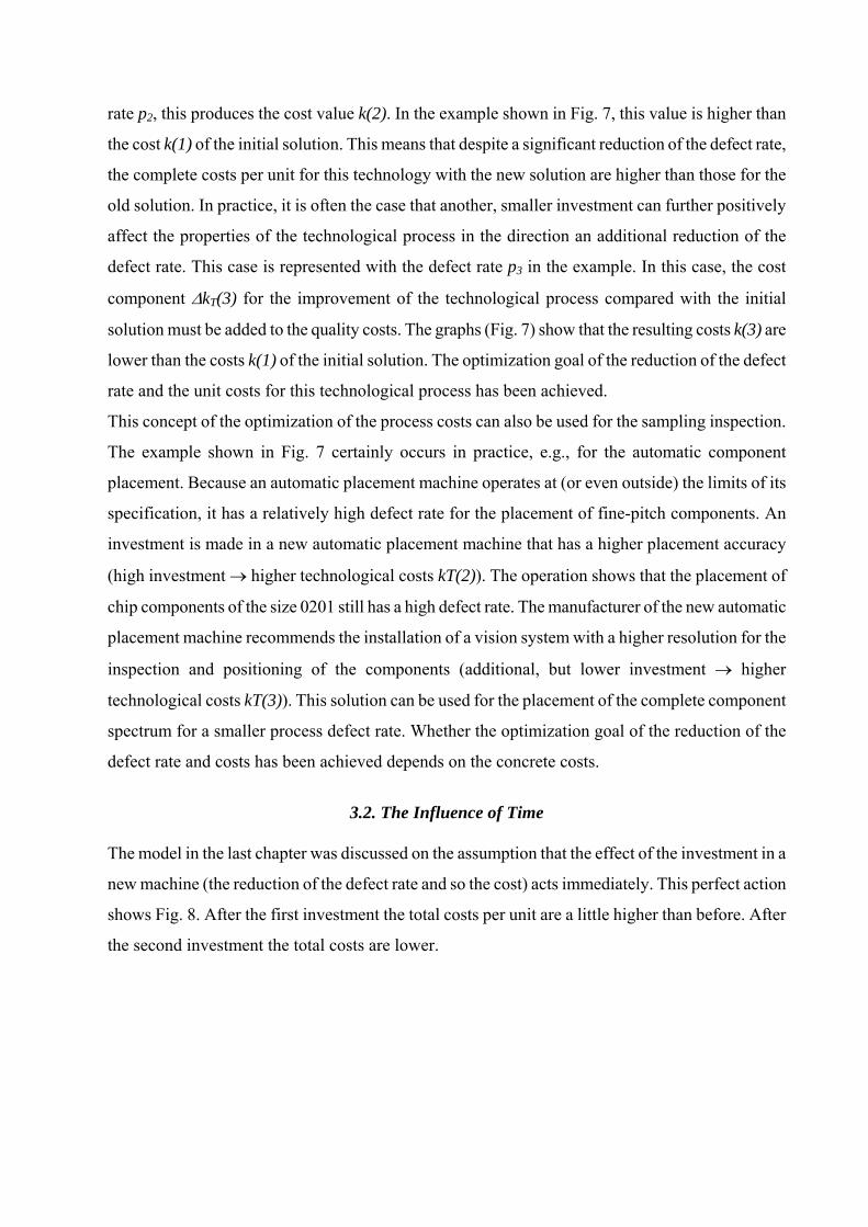
rate p2, this produces the cost value k(2). In the example shown in Fig. 7, this value is higher than

the cost k(1) of the initial solution. This means that despite a significant reduction of the defect rate,

the complete costs per unit for this technology with the new solution are higher than those for the

old solution. In practice, it is often the case that another, smaller investment can further positively

affect the properties of the technological process in the direction an additional reduction of the

defect rate. This case is represented with the defect rate p3 in the example. In this case, the cost

component ΔkT(3) for the improvement of the technological process compared with the initial

solution must be added to the quality costs. The graphs (Fig. 7) show that the resulting costs k(3) are

lower than the costs k(1) of the initial solution. The optimization goal of the reduction of the defect

rate and the unit costs for this technological process has been achieved.

This concept of the optimization of the process costs can also be used for the sampling inspection.

The example shown in Fig. 7 certainly occurs in practice, e.g., for the automatic component

placement. Because an automatic placement machine operates at (or even outside) the limits of its

specification, it has a relatively high defect rate for the placement of fine-pitch components. An

investment is made in a new automatic placement machine that has a higher placement accuracy

(high investment → higher technological costs kT(2)). The operation shows that the placement of

chip components of the size 0201 still has a high defect rate. The manufacturer of the new automatic

placement machine recommends the installation of a vision system with a higher resolution for the

inspection and positioning of the components (additional, but lower investment → higher

technological costs kT(3)). This solution can be used for the placement of the complete component

spectrum for a smaller process defect rate. Whether the optimization goal of the reduction of the

defect rate and costs has been achieved depends on the concrete costs.

3.2. The Influence of Time

The model in the last chapter was discussed on the assumption that the effect of the investment in a

new machine (the reduction of the defect rate and so the cost) acts immediately. This perfect action

shows Fig. 8. After the first investment the total costs per unit are a little higher than before. After

the second investment the total costs are lower.

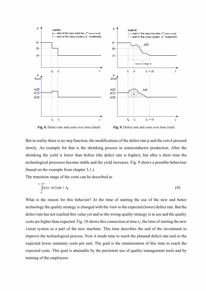
Fig. 8. Defect rate and costs over time (ideal) Fig. 9. Defect rate and costs over time (real)

But in reality there is no step function, the modifications of the defect rate p and the cots k proceed

slowly. An example for that is the shrinking process in semiconductor production. After the

shrinking the yield is lower than before (the defect rate is higher), but after a short time the

technological processes become stable and the yield increases. Fig. 9 shows a possible behaviour

(based on the example from chapter 3.1.).

The transition range of the costs can be described as

(4). k

tt

t

Adtktk =−∫Δ+

ˆ))3()((0

0

What is the reason for this behavior? At the time of starting the use of the new and better

technology the quality strategy is changed with the view to the expected (lower) defect rate. But the

defect rate has not reached this value yet and so the wrong quality strategy is in use and the quality

costs are higher than expected. Fig. 10 shows this connection at time t1, the time of starting the new

vision system as a part of the new machine. This time describes the end of the investment to

improve the technological process. Now it needs time to reach the planned defect rate and so the

expected lower summary costs per unit. The goal is the minimization of this time to reach the

expected costs. This goal is attainable by the persistent use of quality management tools and by

training of the employees.

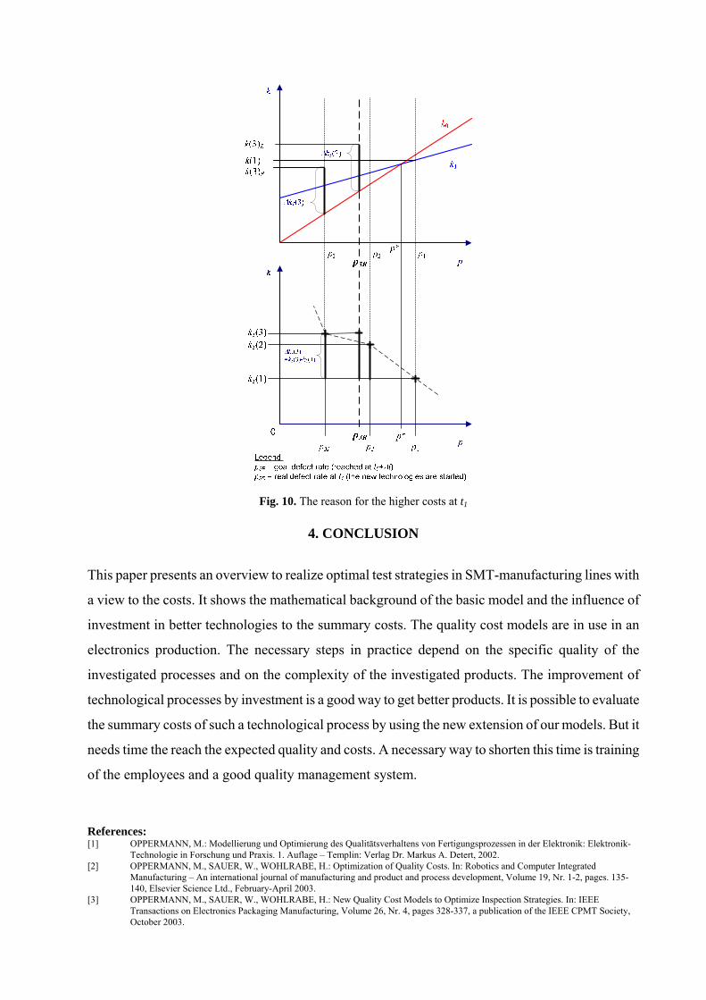
Fig. 10. The reason for the higher costs at t1

4. CONCLUSION

This paper presents an overview to realize optimal test strategies in SMT-manufacturing lines with

a view to the costs. It shows the mathematical background of the basic model and the influence of

investment in better technologies to the summary costs. The quality cost models are in use in an

electronics production. The necessary steps in practice depend on the specific quality of the

investigated processes and on the complexity of the investigated products. The improvement of

technological processes by investment is a good way to get better products. It is possible to evaluate

the summary costs of such a technological process by using the new extension of our models. But it

needs time the reach the expected quality and costs. A necessary way to shorten this time is training

of the employees and a good quality management system.

References: [1] OPPERMANN, M.: Modellierung und Optimierung des Qualitätsverhaltens von Fertigungsprozessen in der Elektronik: Elektronik-

Technologie in Forschung und Praxis. 1. Auflage – Templin: Verlag Dr. Markus A. Detert, 2002. [2] OPPERMANN, M., SAUER, W., WOHLRABE, H.: Optimization of Quality Costs. In: Robotics and Computer Integrated

Manufacturing – An international journal of manufacturing and product and process development, Volume 19, Nr. 1-2, pages. 135-140, Elsevier Science Ltd., February-April 2003.

[3] OPPERMANN, M., SAUER, W., WOHLRABE, H.: New Quality Cost Models to Optimize Inspection Strategies. In: IEEE Transactions on Electronics Packaging Manufacturing, Volume 26, Nr. 4, pages 328-337, a publication of the IEEE CPMT Society, October 2003.

[4] SAUER, W. (Hrsg.): Prozesstechnologie der Elektronik – Modellierung, Simulation und Optimierung der Fertigung. 1. Auflage – München Wien: Carl Hanser Verlag, 2003.

[5] LINSS, G. (Hrsg.): Training Qualitätsmanagement. 1. Auflage – Leipzig: Fachbuchverlag Leipzig im Carl Hanser Verlag München Wien, 2003.

Authors: Dr.-Ing. Martin Oppermann Prof. Dr.-Ing. habil. Wilfried Sauer Technische Universität Dresden Zentrum für mikrotechnische Produktion D-01062 Dresden Tel.: +49 351 463 35051 Fax: +49 351 463 37069 E-mail: oppermann@zmp.et.tu-dresden.de