MAXIMUM POWER POINT TRACKING IN PHOTOVOLTAIC SYSTEMS USING MODEL REFERENCE ADAPTIVE CONTROL

by

Qinhao Zhang

B.S., Shanghai Jiao Tong University, China, 2011

Submitted to the Graduate Faculty of

Swanson School of Engineering in partial fulfillment

of the requirements for the degree of

M.S. in Electrical Engineering

University of Pittsburgh

2012

ii

UNIVERSITY OF PITTSBURGH

SWANSON SCHOOL OF ENGINEERING

This thesis was presented

by

Qinhao Zhang

It was defended on

November 19th, 2012

and approved by

Zhi-Hong Mao, Ph.D., Associate Professor, Department of Electrical and Computer

Engineering

William Stanchina, Ph.D., Professor, Department of Electrical and Computer Engineering

Gregory Reed, Ph.D., Associate Professor, Department of Electrical and Computer

Engineering

Thesis Advisor: Zhi-Hong Mao, Associate Professor, Electrical and Computer Engineering

Department

iii

Copyright © by Qinhao Zhang

2012

iv

This thesis proposes adaptive control architecture for maximum power point tracking

(MPPT) in photovoltaic systems. Photovoltaic systems provide promising ways to generate

clean electric power. MPPT technologies have been used in photovoltaic systems to deliver

the maximum power output to the load under changes of solar insolation and solar panel's

temperature. To improve the performance of MPPT, this thesis proposes a two-layer adaptive

control architecture that can effectively handle the uncertainties and perturbations in the

photovoltaic systems and the environment. The first layer of control is ripple correlation

control (RCC), and the second layer is model reference adaptive control (MRAC). By

decoupling these two control algorithms, the control system achieves the maximum power

point tracking with shorter time constants and overall system stability. To track the maximum

power point as the solar insolation changes, the RCC algorithm computes the corresponding

duty cycle, which serves as the input to the MRAC layer. Then the MRAC algorithm

compensates the under-damped characteristics of the power conversion system: the original

transfer function of the power conversion system has time-varying parameters, and its step

response contains oscillatory transients that vanish slowly. Using the Lyapunov approach, an

adaption law of the controller is derived for the MRAC system to eliminate the under-damped

modes in power conversion.

Keywords: Photovoltaic system, maximum power point tracking, model reference

adaptive control and ripple correlation control.

MAXIMUM POWER POINT TRACKING IN PHOTOVOLTAIC SYSTEMS

USING MODEL REFERENCE ADAPTIVE CONTROL

Qinhao Zhang, M.S.

University of Pittsburgh, 2012

v

TABLE OF CONTENTS

PREFACE ........................................................................................................................... VIII

1.0 INTRODUCTION ................................................................................................... 1

1.1 BACKGROUND ............................................................................................. 1

1.2 MOTIVATION AND PROBLEM STATEMENT ...................................... 3

1.3 RESEARCH HYPOTHESIS ......................................................................... 5

1.4 LITERATURE REVIEW FOR RCC AND MRAC ALGORITHMS ....... 6

2.0 MAIN STRUCTURE OF ENTIRE SYSTEM ...................................................... 9

3.0 DESIGN ANALYSIS FOR MRAC AND RCC .................................................. 14

3.1 SCHEME OF THE MRAC AND PROOF OF STABILITY.................... 14

3.2 RIPPLE CORRELATION CONTROL ..................................................... 26

4.0 RESULTS AND DISCUSSIONS ......................................................................... 30

4.1 SIMULATION SETUP ................................................................................ 30

4.2 STEP RESPONSE OF THE SYSTEM ....................................................... 33

4.3 RESPONSE OF THE SYSTEM USING SINE WAVE INPUT ............... 40

5.0 CONCLUSION AND FUTURE WORK ............................................................ 45

APPENDIX A. MRAC CODING IN THE SIMULATION ............................................... 47

APPENDIX B. DATA COMPARISON CODING .............................................................. 48

BIBLIOGRAPHY .................................................................................................................. 49

vi

LIST OF TABLES

Table 1 Parameters for the simulation ..................................................................................... 32

Table 2 Comparison between the nominal and actual controller parameters .......................... 44

vii

LIST OF FIGURES

Figure 1: I-V and P-V curve for photovoltaic system with different irradiance and

temperature. ............................................................................................................................... 3

Figure 2: The scheme of entire control system ........................................................................ 11

Figure 3: The equivalent small signal circuit of converter. ..................................................... 11

Figure 4: The step response of the under-damped converter. .................................................. 12

Figure 5: The general scheme of the MRAC structure. ........................................................... 15

Figure 6: The proposed MRAC in MPPT. ............................................................................... 19

Figure 7: The step response of the converter. .......................................................................... 33

Figure 8: The step response comparison of plant model I in initial stage. .............................. 35

Figure 9: The step response comparison of plant model II in initial stage. ............................. 35

Figure 10: The step response of plant model II in the initial stage with different PWM input.

.................................................................................................................................................. 36

Figure 11: The step response of plant model I with the input signal analog to the duty cycle.

.................................................................................................................................................. 37

Figure 12: The step response comparison of plant model I after the adaptation stage. ........... 38

Figure 13: The step response comparison of plant model II after the adaptation stage. .......... 39

Figure 14: The error signal comparison for plant model I. ...................................................... 39

Figure 15: The response of plant I in the initial stage. ............................................................. 41

Figure 16: The response of plant II in the initial stage. ........................................................... 42

Figure 17: The error comparison of the sinusoidal input. ........................................................ 42

viii

PREFACE

Firstly, I'd like to extend my sincere appreciation to my committee, my advisor

Professor Mao for his guidance in my academic study and offering me the opportunity to

participate in this exciting research, Professor Stanchina for his trust and valuable

suggestions, and Professor Reed for his generous advice and support.

Secondly, I'd like to extend my thanks to senior graduate student, Raghav Khanna,

who collaborated with me in this project and gave me helpful suggestions. In addition, with

Raghav Khanna's kindly permission, I can use part of the research achievement written in

another paper.

Finally, I'd like to thank my friends and family. They are always supportive and

inspiring to my decision.

1

1.0 INTRODUCTION

1.1 BACKGROUND

Photovoltaic system is a critical component to achieve the solar energy through an

environmentally-friendly and efficient way. Maximum power point tracking algorithm

(MPPT) keeps the photovoltaic systems continuously delivering the maximum power output

to the utility, regardless of the variation in environment condition. Under the effect of MPPT

algorithm, the photovoltaic systems are capable of adapting itself to the environment change

and delivering the maximum power output. Generally, the MPPT controller is embedded in

the power electronic converter systems, so that the corresponding optimal duty cycle is

updated to the photovoltaic power conversion system to generate the maximum power point

output.

A series of the control algorithms for the MPPT are well understood at the present

time, due to the significance of improving the photovoltaic systems performance efficiency.

The underlying principle of maximum power point tracking algorithm is to use the ripple

voltage or current component to identify the variation trend of the power output with the

knowledge of the current versus voltage and the power output versus the voltage of the PV

system. Generally, the operating point for different environment conditions varies and the

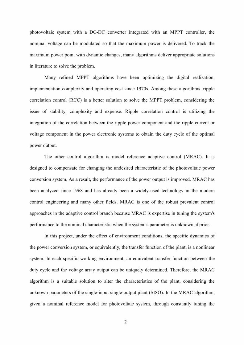
characteristics of the I-V and P-V are generally illustrated in the way shown in Figure 1. The

corresponding voltage array for the maximum power point is varied, as a result of the

variation in the solar insolation and the panel temperatures. By implementing the

2

photovoltaic system with a DC-DC converter integrated with an MPPT controller, the

nominal voltage can be modulated so that the maximum power is delivered. To track the

maximum power point with dynamic changes, many algorithms deliver appropriate solutions

in literature to solve the problem.

Many refined MPPT algorithms have been optimizing the digital realization,

implementation complexity and operating cost since 1970s. Among these algorithms, ripple

correlation control (RCC) is a better solution to solve the MPPT problem, considering the

issue of stability, complexity and expense. Ripple correlation control is utilizing the

integration of the correlation between the ripple power component and the ripple current or

voltage component in the power electronic systems to obtain the duty cycle of the optimal

power output.

The other control algorithm is model reference adaptive control (MRAC). It is

designed to compensate for changing the undesired characteristic of the photovoltaic power

conversion system. As a result, the performance of the power output is improved. MRAC has

been analyzed since 1968 and has already been a widely-used technology in the modern

control engineering and many other fields. MRAC is one of the robust prevalent control

approaches in the adaptive control branch because MRAC is expertise in tuning the system's

performance to the nominal characteristic when the system's parameter is unknown at prior.

In this project, under the effect of environment conditions, the specific dynamics of

the power conversion system, or equivalently, the transfer function of the plant, is a nonlinear

system. In each specific working environment, an equivalent transfer function between the

duty cycle and the voltage array output can be uniquely determined. Therefore, the MRAC

algorithm is a suitable solution to alter the characteristics of the plant, considering the

unknown parameters of the single-input single-output plant (SISO). In the MRAC algorithm,

given a nominal reference model for photovoltaic system, through constantly tuning the

3

parameters of the controller, the characteristics of the plant will converge to the

characteristics of the reference model, meanwhile, the deviation between the reference model

and plant model output will approach to zero, gradually.

Figure 1: I-V and P-V curve for photovoltaic system with different irradiance and temperature.

1.2 MOTIVATION AND PROBLEM STATEMENT

As reported in the given literature, the dynamics of the power conversion system

possesses an under-damped characteristic and the occurrence of oscillation in the transient

period before converging to the nominal voltage output [1]. In term of MPPT, the voltage

output array oscillates back and forth around the nominal voltage value, due to the under-

damped characteristic of the photovoltaic system. Compared with an under-damped system, a

4

critically-damped system converges to the steady state within a shorter time and there is no

oscillation in the transient period. Such result infers that the adapted system will optimize the

voltage response if the MRAC design is used to draw the unknown characteristic of the plant

model to the desired one.

This project proposes a control structure to optimize the performance of the maximum

power point tracking, by coupling two distinct control algorithms together. The first layer of

the system is ripple correlation control algorithm, as briefly introduced in background

Section. The duty cycle for tracking maximum power point under different solar insolation is

obtained within a short time. Then the duty cycle is input into the transistor in the power

conversion system, and its transfer function describes the relationship between the change of

the duty cycle and the change of the array voltage output. The second layer of the system is

model reference adaptive control, which is used to improve the performance of the response

trajectory. Due to the value of the electronic components in the circuit, the transfer function

of the plant is always an unknown parameterized under-damped system and its step response

shows decaying oscillation in the transient period. Under the effect of external condition

changing, it is not feasible to direct tune the system by changing the system's parameters.

Instead, the characteristic of the plant model will converge to the desired characteristic and

the time of tracking maximum power point will be less through the MRAC algorithm,. In

term of the curve of P-V characteristic, the optimized voltage output will display a

straightforward trajectory to the maximum power point without oscillation.

These two control algorithms, as already shown in literature, are independently stable

[2, 3]. However, it is not necessary to infer that the entire coupling system is stability. As a

matter of fact, providing that these two control algorithm's time constant being significantly

disparate, one can decouple these two algorithms so that the overall system is stable for

certainty.

5

In this project, the main object is to design a robust model reference adaptive control

to optimize the performance of maximum power point tracking in order to eliminate the

oscillation during the transient period after the adaptation session. For the main content of

this thesis report, it is primary about the designing procedure, the simulation test analysis and

result discussion of the robust model reference adaptive control. In the future work, the ripple

correlation control will get further improved. Yet, to maintain the integrity of the description

for the entire control system structure, both detailed derivation and analysis of MRAC and

RCC will be shown in the Section 3.

1.3 RESEARCH HYPOTHESIS

More than a hundred documents have well analyzed the improvement of the

photovoltaic systems by solving the MPPT problem; however, quite few attentions have

distributed to the MRAC algorithm. Since the actual external environment change is hard to

model in the simulation, the issue of robustness and stability should be well-considered in the

designing work. To demonstrate the hypothesis of stability and feasibility for entire proposed

control structure, three research goals are set.

Firstly, the research object is to design an MRAC controller to change the unknown

plant characteristic with asymptotically convergence condition. Secondly, by testing the

MRAC designing with different simulation inputs, a valid proof the robustness of the control

system will be established. Thirdly, briefly describing the entire flow of the control system

structure to ensure the entire stability condition being satisfied and the specific

implementation of the system, although, it is quite hard to actually implement the simulation

on the solar panel.

6

This thesis report is the first step of the design for the entire MPPT control system. As

briefly discussed before, in future, series of optimizing analysis will continuously developed

to improve the overall control design. For the rest of this paper, Section 2 will describe the

main structure of the control system. Section 3 will show the design procedure of MRAC and

related educational background of designing issues. Section 4 will demonstrate the robustness

and stability of the control design. Finally, the conclusion of this research is in Section 5.

1.4 LITERATURE REVIEW FOR RCC AND MRAC ALGORITHMS

Several prevalent methods of solving MPPT problem are widely used in the industry.

One algorithm is called the perturb and observe MPPT method (P&O MPPT) [4]. This

method utilizes the additional perturbance component in the voltage or current array to

constantly check whether the system has achieved the nominal current or voltage value. If the

voltage is changed due to a given direction perturbance and the power output increases

simultaneous, it means the maximum power point will be obtained with further such

perturbance for the voltage; on the other hand, if the power output decreases with the same

voltage perturbance, it means the maximum power point can be found with a reversed-

direction perturbance in the current or voltage. Although P&O MPPT algorithm is easy to

implement at an inexpensive cost, this method constantly uses the oscillations to track the

maximum power point even when the system is already in the steady state. The underlying

factor is because P&O MPPT is hard to recognize the source of the perturbance during the

system operating. Sometimes, the perturbance is due to the environment change and

sometimes, it is due to the inherent generated perturbance. As the noise or perturbance always

exists in the system, P&O system can never be stable at the nominal value.

7

The incremental conductance algorithm (INC) [1, 5] locates the maximum power

point, according to the relationship between the power versus voltage, where the derivation of

the power with the voltage is ideally equal to zero. Several literatures have reported its

robustness performance, with the cost of hardware and software complexity. As a matter of

fact, such condition is never exactly satisfied because of the noise, the measurement error and

quantization errors. Meanwhile, INC algorithm also increases the computation time of MPPT

algorithm.

Besides the P&O and the INC algorithms, there are many other advanced algorithms

have been addressed, such as fuzzy logic and the neural network-based algorithms [6, 7].

These methods are suitable for solving certain specific problems; however, the realization of

the system is overwhelmingly complex in the software and hardware construction of the solar

panel. When the maximum power point is obtained, the correlation is equal to zero.

RCC method copes with many drawbacks of other algorithms [3, 8-10]. Several

advantageous features of RCC, comparing to the other given methods have been discussed

and generalized in literature [10]. Briefly, one factor is that RCC has a simple circuit

implementation and fast computation time, compared to the incremental conductance (INC)

method. INC method is also time-consuming in the simulation. Another factor is that RCC

does not need intentional perturbance to generate the ripple component; instead, the

perturbance already exists due to the switching converter in the circuit. Thirdly, the RCC

system is asymptotically converging to the object and its converging rate can be tuned by the

controller gain or the converter switching period. As the consideration of the complexity,

cost, implementation factors, RCC algorithm is recommended to be used in this PV power

conversion system application, although, there is no evident proof to suggest that there be a

best solution in any MPPT problems.

8

Concerning about the method of MRAC, many literature reported the designing

improvement and the specific implementation of MRAC [11-16]. MRAC is derived from the

branch of the model reference control. In the MRC control, with the knowledge of the plant

characteristic, the object is to generate the reference model to improve the performance of the

system output. However, with the knowledge of the plant is unknown to the designer, MRAC

is an alternative way to use the certainty equivalence approach to estimate the plant

parameter. With the different methods used to estimate the plant parameters, different types

of the MRAC will be classified. In this project, the strictly positive real-Lyapunov approach

is preferable in finding the adaptive laws [14-16].

9

2.0 MAIN STRUCTURE OF ENTIRE SYSTEM

In the last section, the two-layer structure of the control system is briefly discussed, as

shown in Figure 2. By mean of the MPPT controller, equivalently RCC algorithm, the duty

cycle is fed into the switching transistor of the converter; hence the maximum power output

can be found. Then through the MRAC component, the transfer function of the converter is

adapted. After the adaptation, the maximum power output will be delivered to the utility.

In this project, it is required to obtain the model of the converter, as shown in Figure

2, which describes the relationship between the dynamics of duty cycle and the voltage

output. When the duty cycle is updated, following by the environment change, the derivation

of the voltage array in the solar panel will be updated as well. To get the transfer function of

the actual plant, one can derive it through the equivalent small signal circuit of the

photovoltaic power conversion system, as detailed shown in Figure 3 [17]:

As shown in Figure 3, the resistor is analog to the solar irradiance or temperature

change with the small signal of the voltage, , to the small signal of the current, . When

the solar insolation changes, the specific operating point of the PV power conversion system

changes, as a result, the value of the resistor varied. And hence the value of the resistor is

unable to predict because it is extremely hard to predict the irradiance of the sun throughout a

day. To obtain the characteristic of the nonlinear system, linearization at a certain operating

point of solar intensity is required. And Figure 3 is the linearization process of the nonlinear

system. As shown in the following, one can express the small signal equivalent circuit of the

system in this way.

10

( )

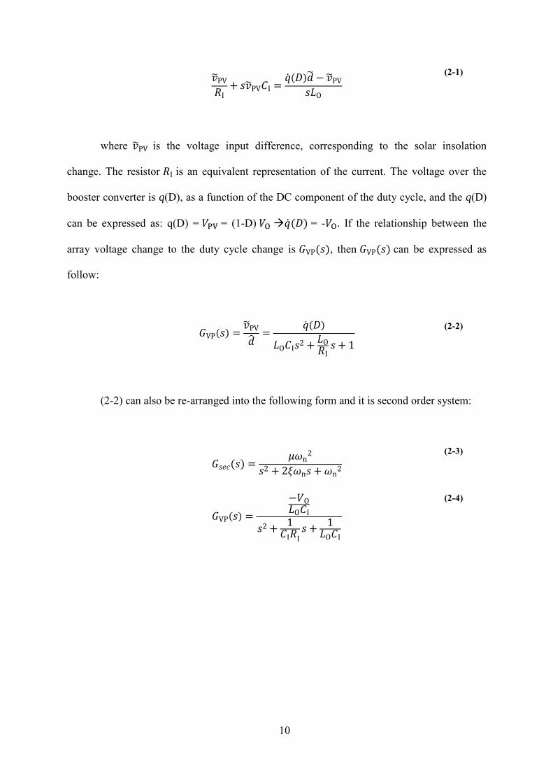
(2-1)

where is the voltage input difference, corresponding to the solar insolation

change. The resistor is an equivalent representation of the current. The voltage over the

booster converter is q(D), as a function of the DC component of the duty cycle, and the q(D)

can be expressed as: q(D) = = (1-D) ( ) = - . If the relationship between the

array voltage change to the duty cycle change is ( ), then ( ) can be expressed as

follow:

( )

( )

(2-2)

(2-2) can also be re-arranged into the following form and it is second order system:

( )

(2-3)

( )

(2-4)

11

Figure 2: The scheme of entire control system.

Figure 3: The equivalent small signal circuit of converter.

12

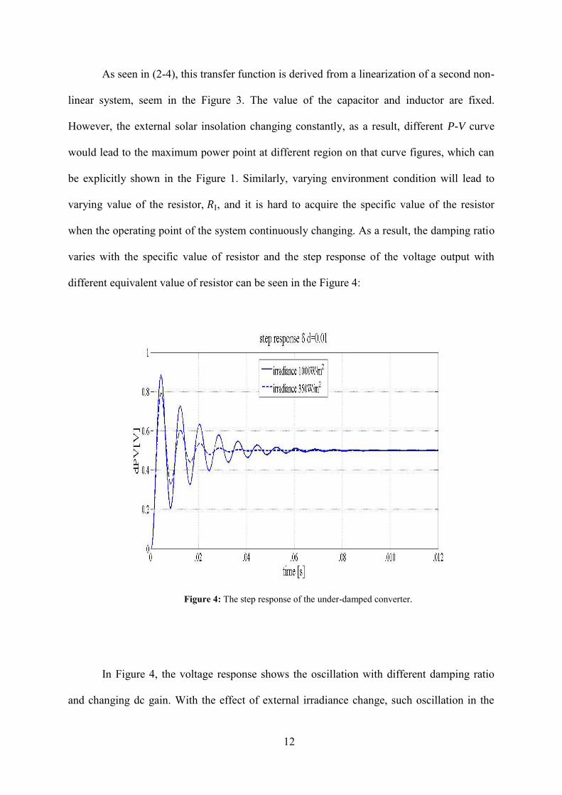
As seen in (2-4), this transfer function is derived from a linearization of a second non-

linear system, seem in the Figure 3. The value of the capacitor and inductor are fixed.

However, the external solar insolation changing constantly, as a result, different P-V curve

would lead to the maximum power point at different region on that curve figures, which can

be explicitly shown in the Figure 1. Similarly, varying environment condition will lead to

varying value of the resistor, , and it is hard to acquire the specific value of the resistor

when the operating point of the system continuously changing. As a result, the damping ratio

varies with the specific value of resistor and the step response of the voltage output with

different equivalent value of resistor can be seen in the Figure 4:

Figure 4: The step response of the under-damped converter.

In Figure 4, the voltage response shows the oscillation with different damping ratio

and changing dc gain. With the effect of external irradiance change, such oscillation in the

13

transient period inevitable occurs and the various time constant for each distinct system

which corresponds to the sunshine intensity, will significantly extend the converging rate of

the converter and in the most time the system cannot deliver the maximum power output.

Besides, there is no straightforward approach to estimate the parameters in the transfer

function of the plant to change the characteristics of the plant and eliminate oscillation during

the transient period. Therefore, it is necessary to use the mechanism of MRAC to solve the

difficulty and improve the output performance of the system. Since the parameter of the

transfer function, as shown in the (2-4), is changing swiftly, the Lyapunov-based direct

MRAC algorithm is recommended to design a stable control structure to tune the plant. The

related details and analysis will be extensively discussed as following.

14

3.0 DESIGN ANALYSIS FOR MRAC AND RCC

3.1 SCHEME OF THE MRAC AND PROOF OF STABILITY

As discussed in Section 2 that the transfer function between the duty cycle and the

voltage output in the array is an under-damped second order system. When the updated duty

cycle inputs into dynamic system, the voltage output will display decaying oscillation in the

transient period and gradually converge to the nominal voltage of the maximum power point.

It is desired that the transfer function has the critically-damped characteristic, not only

because the time constant will be minimized compared to the time constant of the under-

damped system, but also no oscillation will occur in the transient response. To obtain a

critically damped response for the given transfer function, the general MRAC architecture is

shown in the Figure 5.

The input to the overall system, r is the duty cycle obtained in the ripple correlation

control method. The specific transfer function of the plant model, or equivalently the system

of photovoltaic power conversion, can be obtained in the following section. Also, it is

certainly that the transfer function of the plant model is a second order system and the relative

degree of the system is two. The fundamental object of MRAC used in this project is to draw

the characteristic of the plant to the characteristics of the reference model. By designing an

ideal reference model, after adaptation, the plant model will have such characteristics as well.

The result of each iterative comparison, between the plant and reference model output is the

error signal. The error signal as well as the input and the output of the plant, adaptively

15

enable the adjustment parameters to tune the controller so that the parameters of the plant will

converge to the parameters of the reference model. Eventually, the error between the plant

and the reference model will drive to zero and the controller parameters will converge to the

nominal controller parameters, so that the full convergence is achieved and thus the adapted

array voltage tracks the theoretical MPP voltage. It is desired that the plant deliver a critically

damped response under the essential condition that the input signal is persistently exciting.

Figure 5: The general scheme of the MRAC structure.

Generally, for any signal, u(t), is considered as persistently exciting if the following

condition is satisfied:

∫ ( )

(3-1)

16

in (3-1), for any positive value t, there exists and to meet the condition, then the

signal u(t) satisfies the PE condition. It is also necessary to interpret that the input signal

should be 2n order with a given nth order plant model. In the simulation, it is instructive to

know that the combination of step function and sin function are all satisfied with the PE

condition.

In the general MRAC architecture, quite many different methods can be utilized to

find the adaptive laws for the controller to make sure the error signal converge. Basically, the

prevalent method at the present is using Lyapunov function to ensure the system converge

asymptotically. There are several definitions to determine the meaning of stability in the

control theory. The stability in the sense of Lyapunov is a mild approach to find the adaptive

law by ensuring the asymptotic stability. An arbitrary point is stable if for any >0, there

always exists a value >0, so that the norm value between the current point and the nominal

equilibrium point is always less than the . In other word, the stability in the sense of

Lyapunov is independent of the initial condition of the system and is significantly sufficient

to guarantee the stability. As shown in Section 2, the relative degree plant of the photovoltaic

power conversion system e.g. (deg( )-deg( )) is two. The transfer functions for the

reference model is ( ) and the plant model is ( ), they can be represented as seen in

(3-2):

( )

( )

( )

( )

( )

( )

(3-2)

where and are the chosen gain of the systems, and , , and are the

chosen parameters of the reference model and the plant model. By tuning the parameters in

17

(3-2), a critical damping system can be obtained under the condition being satisfied:

√ . Several assumptions about (3-2) should be announced before the further

analysis:

• the numerator and the denominator of polynomial in (3-2) are monic Hurwitz.

• the reference model is controllable and observable.

• the relative degree of (3-2) are the same and it is known.

• the degree of denominator of plant and the sign of the gain, , is known.

• both the reference model and the plant model are controllable and observable

The expression for the controller is the combination of the input, output of the plant

and the input of the reference model, as seen in (3-3):

( )

( )

( )

( )

(3-3)

In (3-3), is the input to the plant, vector is the parameter vector

of the controller, which is updated through the adaptive law which is required to find.

Furthermore, r and are the input to the system and the output of the plant, respectively,

while ( )

( ) is a arbitrarily designed nth (deg( )-1) order stable filter as denoted in Figure 6.

The filter is used to ensure the stability of the system through derivative operation in the

high-order system. Actually, in the practical situations, the only available variables to be

measured are the the input of the system, the output of the reference model and of the plant.

Therefore, other forms of intermediate variables, such as high order differentiation of the

output is hard to measure and the derivation operating will lead the system to be unstable and

is unobservable. The polynomial ( ) contains the polynomial ( ), the numerator of the

transfer function for the reference model, and the expression of the polynomial is: ( )

18

( ) ( ). In the state variable vector , variable is equal to ( )

( )

and variable is equal to ( )

( ) . To obtain the controller's parameter and converge the plant

model to the reference model, one can substitute r for , according to the relationship in

(3-3). Then the transfer function between the input of the system, r and the output of the

plant, ., can be obtained in (3-4):

( ) ( )

( )( ( ) ( )) ( ) ( ) ( ) ( )

(3-4)

In the (3-4), there is one zero and three poles for the transfer function. Sometimes, it is

hard to guarantee that the overall transfer function of the plant after the controller tuning still

has the same order as previously, instead, some plant will be transformed into a new plant

with the same relative degree and higher order. It is hard to recognize such changing by

measuring those variables; nevertheless, it maybe jeopardizes the stability condition of the

entire system. With those assumptions claimed before, it is ensured that there is one

additional pole and zero cancellations in the overall system and the order and characteristic of

the transfer function for the converter remain. Equating (3-4) to the transfer function of the

reference model in (3-2), the characteristics of the plant will share the same characteristics of

the reference model if the following conditions listed in (3-5) are satisfied:

{

( )( ( ) ( )) ( ) ( ) ( ) ( )

( ) ( ) ( ) ⇒

(3-5)

19

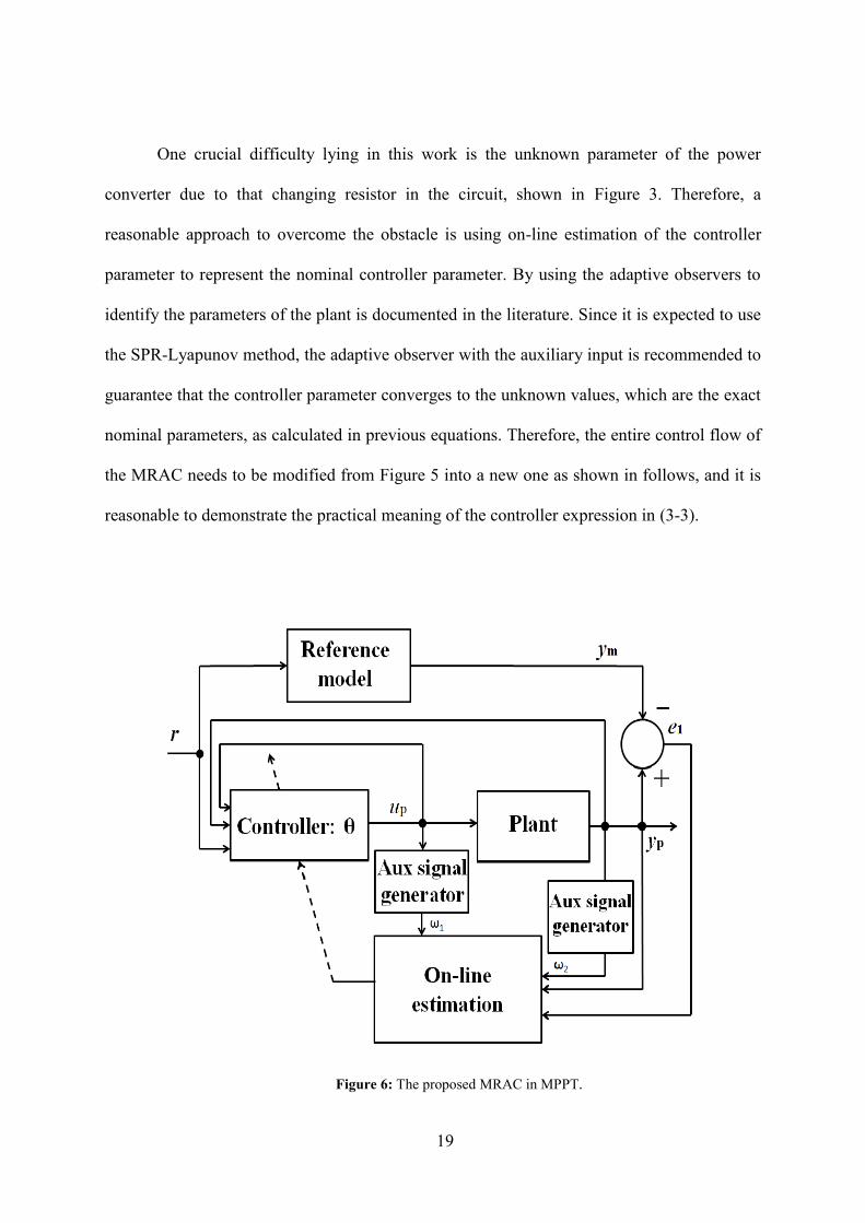
One crucial difficulty lying in this work is the unknown parameter of the power

converter due to that changing resistor in the circuit, shown in Figure 3. Therefore, a

reasonable approach to overcome the obstacle is using on-line estimation of the controller

parameter to represent the nominal controller parameter. By using the adaptive observers to

identify the parameters of the plant is documented in the literature. Since it is expected to use

the SPR-Lyapunov method, the adaptive observer with the auxiliary input is recommended to

guarantee that the controller parameter converges to the unknown values, which are the exact

nominal parameters, as calculated in previous equations. Therefore, the entire control flow of

the MRAC needs to be modified from Figure 5 into a new one as shown in follows, and it is

reasonable to demonstrate the practical meaning of the controller expression in (3-3).

Figure 6: The proposed MRAC in MPPT.

20

As shown in Figure 6, the input and the output of the plant model are fed into the

observer, so that the auxiliary signal and are joined into the on-line estimation to

tuning the controller parameters. Therefore, several consequence need to be noticed: firstly,

the parameter vector of the controller will be changed into the estimation parameter vector,

. Secondly, with the realization of the adaptive observers in this system, the following

properties can be guaranteed with the PE conditioned input:

• all the signals in the system are uniformly bounded

• the error between the actual output of the plant model and the estimated output of

the plant model will approach to zero as time goes to infinity

• the error between the state space realization of the plant model and the estimated

realization will converge to zero exponentially fast as time goes infinity.

By iteratively using the output of the reference model and the plant, the controller

parameters converge to the nominal parameters. Thus, the form of in (3-3) can be

expressed as seen in (3-6):

(3-6)

Arbitrarily choosing ( ) and hence ( )

( )

and

( )

( )

. These two state observers equations can be represented as shown in (3-7):

{ ( )

( ) (3-7)

21

The observers in (3-7) are implemented to estimate the minimal realization of the

plant to obtain the error between the reference model output and the plant model output [13].

The state-space realization of the transfer function for the plant and reference model, shown

in (3-2), can be decomposed into the state space equation, shown as follows:

{

( )

( ) ( )

( )

( )

( )

(3-8)

By substituting the input of the plant mode, , with the controller expression, the

state space of the plant model in (3-8) can be obtained:

⇒ {

(

)

(3-9)

Since the object of the plant realization, shown in (3-9), is to be equal to the

realization of the reference model under the factor of the controller, then the plant model,

after the tuning, has owned the same state space realization as the realization of the reference

model. Then the state-space equation for the overall closed-loop plant can be achieved by

augmenting the state of the plant with the states , of the controller. Combining the

controller expression in (3-3) with the observers equations in (3-7), the state-space equation

model for the plant and reference model is obtained:

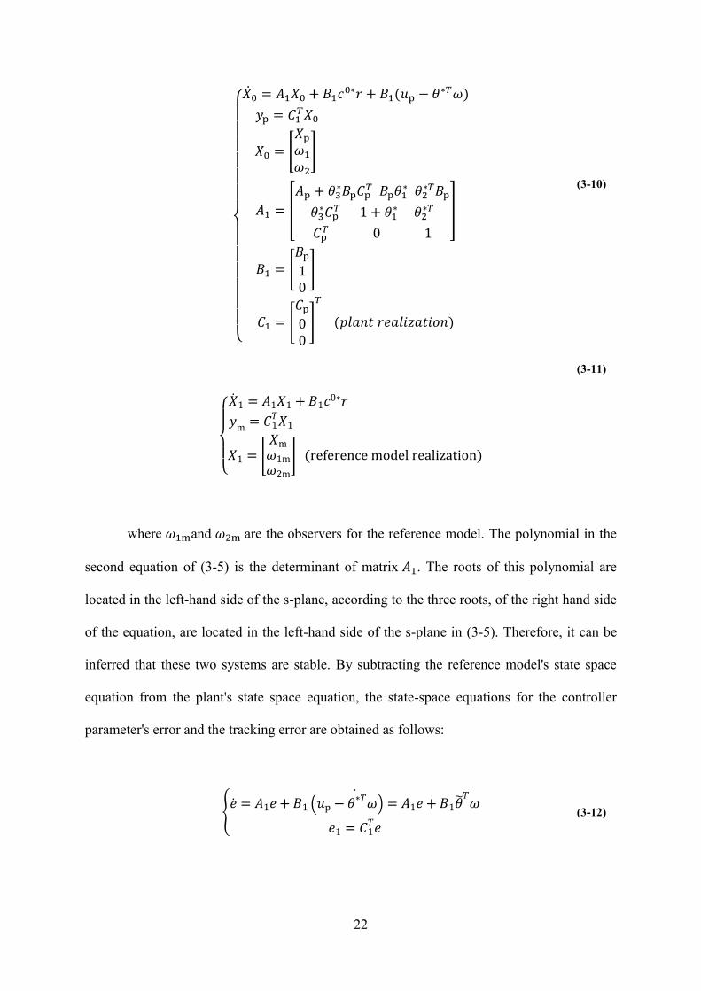
22

{

( )

[

]

[

]

[

]

[

]

( )

(3-10)

{

[

] ( )

(3-11)

where and are the observers for the reference model. The polynomial in the

second equation of (3-5) is the determinant of matrix . The roots of this polynomial are

located in the left-hand side of the s-plane, according to the three roots, of the right hand side

of the equation, are located in the left-hand side of the s-plane in (3-5). Therefore, it can be

inferred that these two systems are stable. By subtracting the reference model's state space

equation from the plant's state space equation, the state-space equations for the controller

parameter's error and the tracking error are obtained as follows:

{ ( )

(3-12)

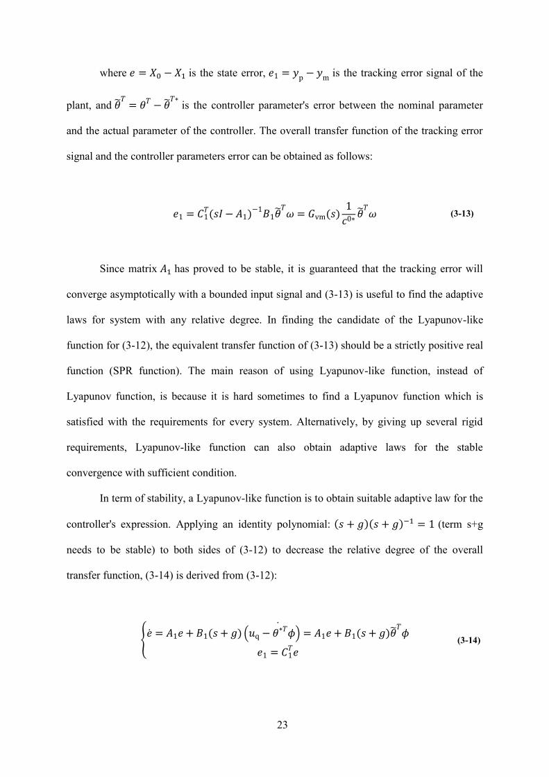
23

where is the state error, is the tracking error signal of the

plant, and

is the controller parameter's error between the nominal parameter

and the actual parameter of the controller. The overall transfer function of the tracking error

signal and the controller parameters error can be obtained as follows:

( )

( )

(3-13)

Since matrix has proved to be stable, it is guaranteed that the tracking error will

converge asymptotically with a bounded input signal and (3-13) is useful to find the adaptive

laws for system with any relative degree. In finding the candidate of the Lyapunov-like

function for (3-12), the equivalent transfer function of (3-13) should be a strictly positive real

function (SPR function). The main reason of using Lyapunov-like function, instead of

Lyapunov function, is because it is hard sometimes to find a Lyapunov function which is

satisfied with the requirements for every system. Alternatively, by giving up several rigid

requirements, Lyapunov-like function can also obtain adaptive laws for the stable

convergence with sufficient condition.

In term of stability, a Lyapunov-like function is to obtain suitable adaptive law for the

controller's expression. Applying an identity polynomial: ( )( ) (term s+g

needs to be stable) to both sides of (3-12) to decrease the relative degree of the overall

transfer function, (3-14) is derived from (3-12):

{ ( ) ( ) ( )

(3-14)

24

where several new state variables are introduced:

,

. The term s+g will be absorbed into the matrix . Since ,

equivalently, the controller's input can be updated as:

(3-15)

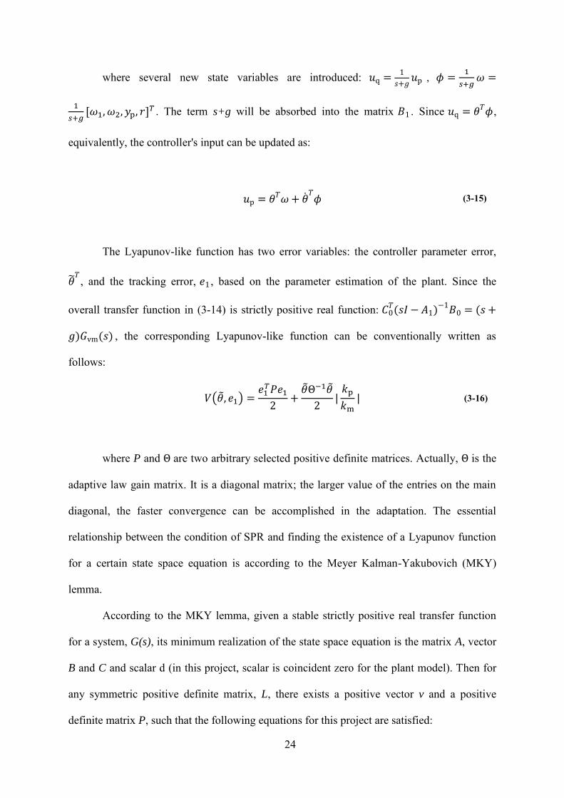
The Lyapunov-like function has two error variables: the controller parameter error,

, and the tracking error, , based on the parameter estimation of the plant. Since the

overall transfer function in (3-14) is strictly positive real function: ( )

(

) ( ) , the corresponding Lyapunov-like function can be conventionally written as

follows:

( )

(3-16)

where P and are two arbitrary selected positive definite matrices. Actually, is the

adaptive law gain matrix. It is a diagonal matrix; the larger value of the entries on the main

diagonal, the faster convergence can be accomplished in the adaptation. The essential

relationship between the condition of SPR and finding the existence of a Lyapunov function

for a certain state space equation is according to the Meyer Kalman-Yakubovich (MKY)

lemma.

According to the MKY lemma, given a stable strictly positive real transfer function

for a system, G(s), its minimum realization of the state space equation is the matrix A, vector

B and C and scalar d (in this project, scalar is coincident zero for the plant model). Then for

any symmetric positive definite matrix, L, there exists a positive vector v and a positive

definite matrix P, such that the following equations for this project are satisfied:

25

{

(3-17)

Based on the knowledge of MKY lemma, the derivation of the Lyapunov-like

function seen in (3-16) along the solution of (3-14) is expressed as:

( )

(3-18)

According to the definition of the stability in sense of Lyapunov stability, if the

differentiation of the function ( ) is less then zero, then the system is uniformly

asymptotically stable. As seen in the (3-18, to find the adaptive law for the error of the

controller parameter, it is suggested that the polynomial

be

equal to zero will result (3-18 less than zero because of the polynomial:

less than zero. The system's output error and the controller parameter error are

guaranteed to converge asymptotically to zero based on the controller parameter's updated

law, as shown in (3-19):

(3-19)

[

( )

( )

]

Since the matrix is stable and the equivalent transfer function of the error of the

output and the controller parameter, shown in (3-14) is strictly positive real function, it can be

inferred that the error of the system output and the parameter error of the controller will

converge asymptotically to zero, with the bounded source of the input, system output error

and the choice of state variable vector. According to the derivations above, the overall

26

MRAC adaptive rules can be concluded as follows and each item in (3-20) is the function

with zero value initial conditions:

{

(3-20)

A series of adaptive control updating laws are obtained in (3-20). With the entire

scheme of MRAC found, two important conceptions are instructive to be informed: firstly,

signal in the closed-loop plant is bounded and the tracking error signal will converge to zero

asymptotically. Secondly, if the numerator and the denominator of the plant is coprime and

the input signal is sufficiently rich of order, the tracking error signal will converge

exponentially fast.

3.2 RIPPLE CORRELATION CONTROL

To deliver the maximum power output to the load at the steady state, RCC algorithm

is utilized to calculate the duty cycle. RCC algorithm was recently developed and reported in

[2, 3, 9, 18], where it was shown that the switching transistor will result in an inherent ripple

voltage or current component, which can be utilized to track the location of the maximum

power point. As briefly introduced in the Section 1.1, RCC algorithm is an improved

algorithm based on the P&O method, because it avoids external energy to generate the

27

voltage ripple for tracking the MPP. In additional, it is proven in the report that RCC

algorithm is asymptotically convergence to the MPP. As shown in the Figure 1, there is only

one peak power value in the PV curve or the PI curve, where the maximum power delivery is

obtained. Correlating the derivation of the power output and the derivation of the voltage

output, the correlation identifies whether the present voltage is lower or higher than the

nominal voltage output. To mitigate the array capacitance in the circuit, it is desired to use the

ripple voltage component in the correlation, as the following formula to calculate the duty

cycle shown:

{

(3-21)

The control law can be seen in (3-22), as:

∫ (3-22)

where and are the ripple component of the array power and voltage, and k is

the negative valued gain. (3-22) can be described as follows: if increases and it result an

increasing , the system's operating point is located on the left side of the MPP, therefore

the value of d is decreasing; similarly, if increases and it result a decreasing , the

system's operating point is located on the right side of the MPP. Inspecting (3-21) and (3-22),

the maximum power point can be obtained when the derivation of d is equal to zero because

that is the place where the voltage array is equal to the nominal one and the change of d can

be assumed to zero. Given the mathematically proof for the stability of the RCC algorithm,

the corresponding duty cycle for the maximum power point under various solar insolations

28

can be achieved. In the RCC algorithm, the underlying principle is using whatever ripple is

already presented in the system to determine the location of the maximum power point.

Alternatively, the control algorithm by mean of the ripple current component can be

realized as well because the P-I curve and P-V curve are similar to each other. One

modification is the sign of the gain value of k needs to be reversed. However, due to the

practical implementation, the issue of the parasite capacitor is necessary to be considered, the

voltage ripple component is obviously advantageous than the current ripple component. As

inferred from the literature review in Section 1, many improved and alternative version of

RCC algorithms have been developed to replace the original one, another way to propose the

RCC algorithm is using the direct integrand of the ratio between the power output and the

ripple component of the voltage or the power output and the ripple component of the current:

∫

(3-23)

the control law in (3-23) is hard to expect working due to the complexity of realizing

the integrand of this ratio in the circuit. Moreover, like the drawback of P&O MPPT

algorithm, the ratio of signal-to-noise is unavailable and hence the (3-23) is not sufficient to

make the judgment that the duty cycle for the maximum power point is achieved because the

ratio between the ripple power and voltage component is impossible to maintain ideally being

zero for quite amount of time. Due to the effect of noise, this control law is not reliable to

make the determination.

With increasing focus on the simple implementation of the algorithm in circuit, one

useful control law makes use of the sign function to track the MPP in the circuit. As shown

the control law is:

29

∫ (

) (

) (3-24)

the effect of noise is mitigated because of the sign function only focus on whether the

derivation of d is larger, smaller or equal to zero. And this control law is easy to realize in

electronics hardware by using logic circuit at an inexpensive cost. This control law was also

proved mathematically that it is stable, and thus it is an alternative RCC algorithm to be used

in this project.

30

4.0 RESULTS AND DISCUSSIONS

It is recommended to notice that when two distinct control algorithms decoupling

together, it is not necessary to infer that the overall system is stable. However, as reported in

the literature and analysis, the time constant of the two control methods are significantly

disparate: RCC is several milliseconds and the MRAC is several seconds. Thus, when

decoupling these two control algorithms together, the overall system will be stable for sure.

4.1 SIMULATION SETUP

In the project simulation, based on the given literature, the duty cycle is easily

obtained and to be the input of the following MRAC system. The input of the system is

modeled as two types signal function: one is the step function and the combination of step

function, where the first one can be analog to the abrupt change of sunshine strength or the

solar panel's temperature drop or jump in the practical situation and the latter one can be used

to simulate the digital output of the RCC with short sample rate; the other type is the

combination of several sine wave functions, which is generally analog to the smooth

changing of the external environment changing in the most cases. These two types of input

test the system from the view of magnitude and frequency characteristic. And the inputs are

satisfied with the condition of persistence exciting.

31

Analytically, when the characteristics of the plant and the reference model are

explicitly known as in the format of (3-2), the nominal controller parameter vector, can be

easily obtained, through equating (3-2) to (3-6) and choosing a stable filter ( )

(variable a is any positive real number). The nominal parameters of the controller are seen

in (3-21):

{

( )( )

( ) ( )( )

(4-1)

Providing the knowledge of these parameters, it is easy for the designer to see

whether the MRAC structure works in the expecting scenario that the estimated controller

parameter converges to the nominal parameters of the controller obtained in (4-1). This

design could be realized in circuit, nevertheless, the simulation is set up in Simulink and the

simulation time is approximately normalized into the actual time.

In the simulation, the reference model is designed to be a critically-damped second-

order system and the plant is an under-damped second-order system. In selecting the

parameters for the critically damped reference model, the damping ratio of

√ is the

determining factor as inferred in (3-2). Normally, the damping ratio for the critical damped

system is chosen to be either exact one or slightly less than one, because the system's

converge rate will be improved at the cost of slightly overshoot in the transient period of the

output response. Secondly, the natural frequency of the plant is fixed by the selection of the

capacitor and the inductor in Figure 3, which can be expressed as: √

. From the view of

32

energy saving and fast convergence, the natural frequency of the reference model is

suggested to be close to the natural frequency of the plant model. Thirdly, to make the

algorithm easy to implement, the dc gain of the reference model is suggested to design

equally to the dc gain of the plant model. So that the system will not require extra control

method to make the system responses of the reference model and plant model have the exact

same curve shape. Upon these considerations, the parameters of the reference model are

selected as following.

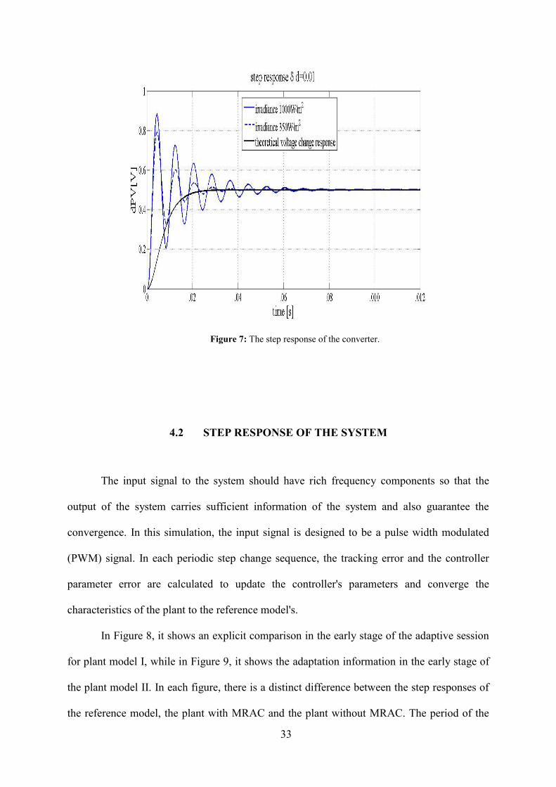
To overly test the performance of the MRAC controller design, two plant models are

arbitrarily designed. As seen in Table 1, the damping ratio for the plant model II is much

smaller than the damping ratio for the plant model I, as a result, the characteristic of plant

model I is different from the characteristic of plant model II. As shown in Figure 7, the plant

model II converges to the nominal voltage output swiftly and the envelop of the oscillation in

plant model I decays slowly. By tuning these two plant models with significantly

characteristic differences, the conclusion of the designed MRAC performance is adequate for

the validity.

Table 1: Parameters for the simulation

Parameter Reference model Plant model I test Plant model II test

9 9 9

6 0.2 0.006

9 9 9

1 1 1

damping ratio 1 0.0333 0.001

33

Figure 7: The step response of the converter.

4.2 STEP RESPONSE OF THE SYSTEM

The input signal to the system should have rich frequency components so that the

output of the system carries sufficient information of the system and also guarantee the

convergence. In this simulation, the input signal is designed to be a pulse width modulated

(PWM) signal. In each periodic step change sequence, the tracking error and the controller

parameter error are calculated to update the controller's parameters and converge the

characteristics of the plant to the reference model's.

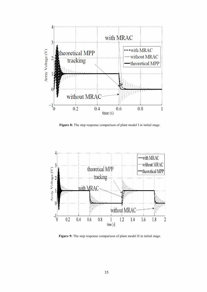
In Figure 8, it shows an explicit comparison in the early stage of the adaptive session

for plant model I, while in Figure 9, it shows the adaptation information in the early stage of

the plant model II. In each figure, there is a distinct difference between the step responses of

the reference model, the plant with MRAC and the plant without MRAC. The period of the

34

pulsed modulated width signal is 1.2 seconds. In the first 0.6 second, the voltage output

without using MRAC displays decaying oscillation and gradually converges to the nominal

voltage value in approximate 0.3 second. On the other, in the initial stage, under the effect of

the controller, there are significant oscillates for the system using MRAC in the voltage

output and it illustrates the maximum derivation, which is even larger than the derivation

between the output of the plant model without using MRAC and the output of the reference

model. The maximum derivation between the plant model using MRAC and the reference

model occurs after around 0.03 second. After that, the oscillation of the step response for the

adapted plant converges to the steady state for another 0.06 second. It seems that the plant has

been tuned to acquire similar characteristic of the step response for the reference model and

the time duration of such adaptation is very short, and this time constant is even shorter than

the time constant of the plant model without using MRAC. As illustrated in the next half

period where the state changing from one back to zero, the voltage output approaches to

steady state without any oscillations and the approaching curve is close to the curve of the

reference model's response.

By comparing Figure 8 and Figure 9, it is surprisingly to find that the initial

adaptation process for two plant model is quite similar to each other. With the same control

structure of MRAC, the convergence of the characteristic of plant model is exponentially fast.

35

Figure 8: The step response comparison of plant model I in initial stage.

Figure 9: The step response comparison of plant model II in initial stage.

36

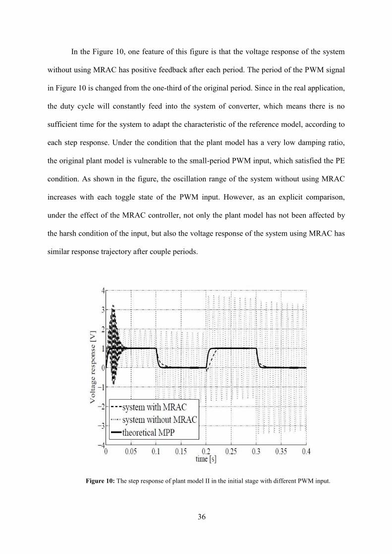
In the Figure 10, one feature of this figure is that the voltage response of the system

without using MRAC has positive feedback after each period. The period of the PWM signal

in Figure 10 is changed from the one-third of the original period. Since in the real application,

the duty cycle will constantly feed into the system of converter, which means there is no

sufficient time for the system to adapt the characteristic of the reference model, according to

each step response. Under the condition that the plant model has a very low damping ratio,

the original plant model is vulnerable to the small-period PWM input, which satisfied the PE

condition. As shown in the figure, the oscillation range of the system without using MRAC

increases with each toggle state of the PWM input. However, as an explicit comparison,

under the effect of the MRAC controller, not only the plant model has not been affected by

the harsh condition of the input, but also the voltage response of the system using MRAC has

similar response trajectory after couple periods.

Figure 10: The step response of plant model II in the initial stage with different PWM input.

37

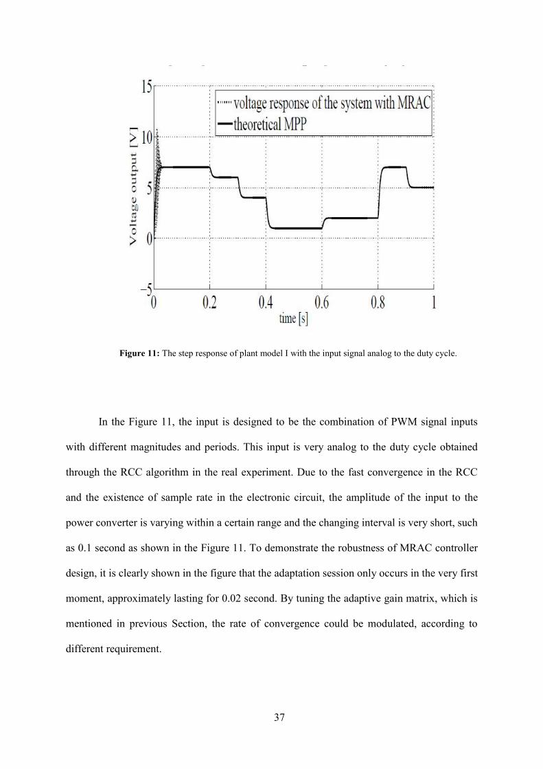
Figure 11: The step response of plant model I with the input signal analog to the duty cycle.

In the Figure 11, the input is designed to be the combination of PWM signal inputs

with different magnitudes and periods. This input is very analog to the duty cycle obtained

through the RCC algorithm in the real experiment. Due to the fast convergence in the RCC

and the existence of sample rate in the electronic circuit, the amplitude of the input to the

power converter is varying within a certain range and the changing interval is very short, such

as 0.1 second as shown in the Figure 11. To demonstrate the robustness of MRAC controller

design, it is clearly shown in the figure that the adaptation session only occurs in the very first

moment, approximately lasting for 0.02 second. By tuning the adaptive gain matrix, which is

mentioned in previous Section, the rate of convergence could be modulated, according to

different requirement.

38

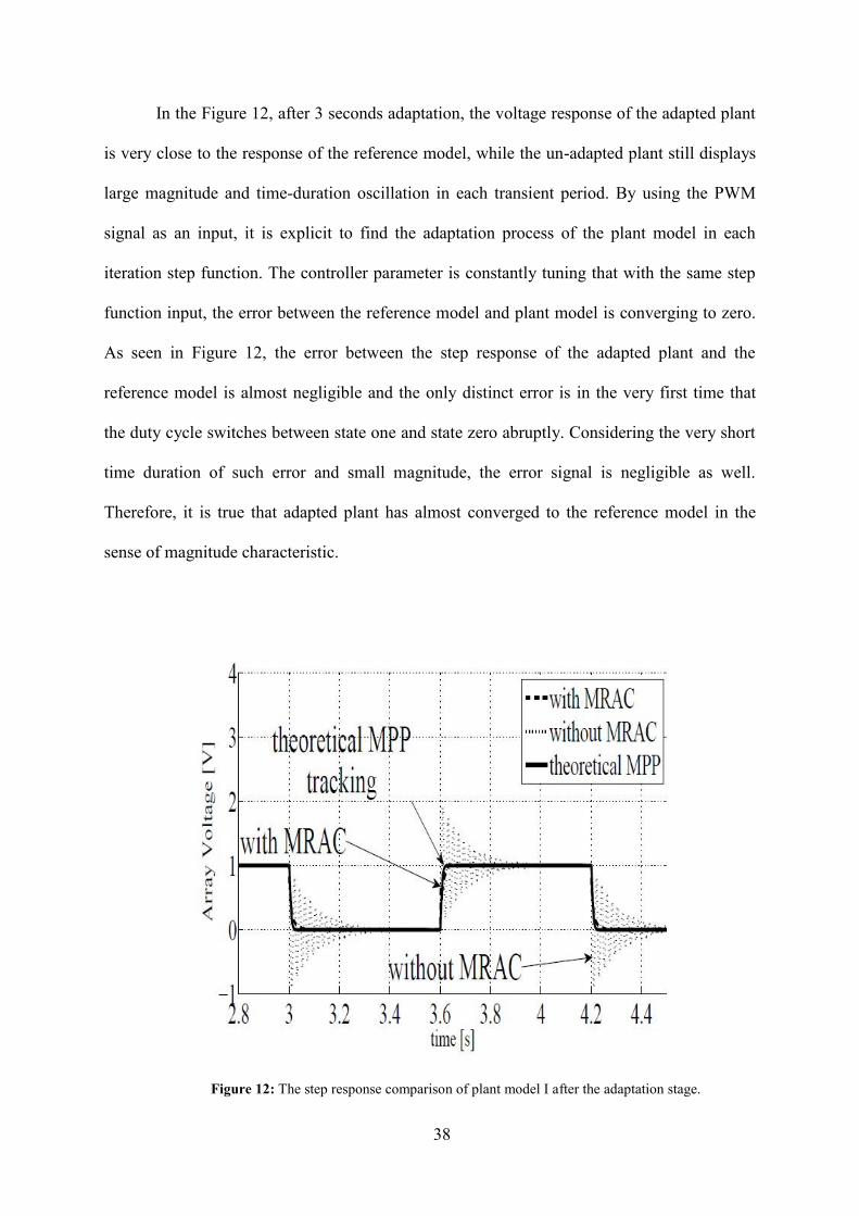
In the Figure 12, after 3 seconds adaptation, the voltage response of the adapted plant

is very close to the response of the reference model, while the un-adapted plant still displays

large magnitude and time-duration oscillation in each transient period. By using the PWM

signal as an input, it is explicit to find the adaptation process of the plant model in each

iteration step function. The controller parameter is constantly tuning that with the same step

function input, the error between the reference model and plant model is converging to zero.

As seen in Figure 12, the error between the step response of the adapted plant and the

reference model is almost negligible and the only distinct error is in the very first time that

the duty cycle switches between state one and state zero abruptly. Considering the very short

time duration of such error and small magnitude, the error signal is negligible as well.

Therefore, it is true that adapted plant has almost converged to the reference model in the

sense of magnitude characteristic.

Figure 12: The step response comparison of plant model I after the adaptation stage.

39

Figure 13: The step response comparison of plant model II after the adaptation stage.

Figure 14: The error signal comparison for plant model I.

40

In Figure 14, it shows the tracking error over the time. One is the error between the

output of the plant with MRAC and the reference model; the other one is the error between

the output of the plant without using MRAC and the reference model. As seen in Figure 14,

in the first stage, the thick line error signal is significant because of the adaptation process.

However, as the plant continues to learn during the adaptive session, after 0.1 seconds, the

error signal converges into a much smaller range and ultimately converges to zero. For each

0.6 second, the error signal strike for a very short time due to the abrupt change at each step,

and then remain zero afterward. As time goes, the error strike decreases in magnitude and

time duration.

4.3 RESPONSE OF THE SYSTEM USING SINE WAVE INPUT

Figure 15, Figure 16 and Figure 17 are the set of comparisons of the plant model

using the sine wave function. In Figure 15 and Figure 16, one signal is the theoretical voltage

output with the reference model; the other two are the outputs from the system using MRAC

and without using MRAC. The input of the simulation consists of three frequency

components. The output response of the system at the steady state will display stable

frequency components, namely, each period will highlight the frequency characteristic. As

shown in Figure 15, the output response of the system using MRAC obtains the frequency

characteristic of the reference model after the first period. However, the output response of

the system, without using MRAC, shows disparate frequency characteristic. By comparing

the Figure 15 and Figure 16, it is shown that the system with using MRAC has a quite similar

response curve shape and has a shorter time constant to convergence to the frequency steady

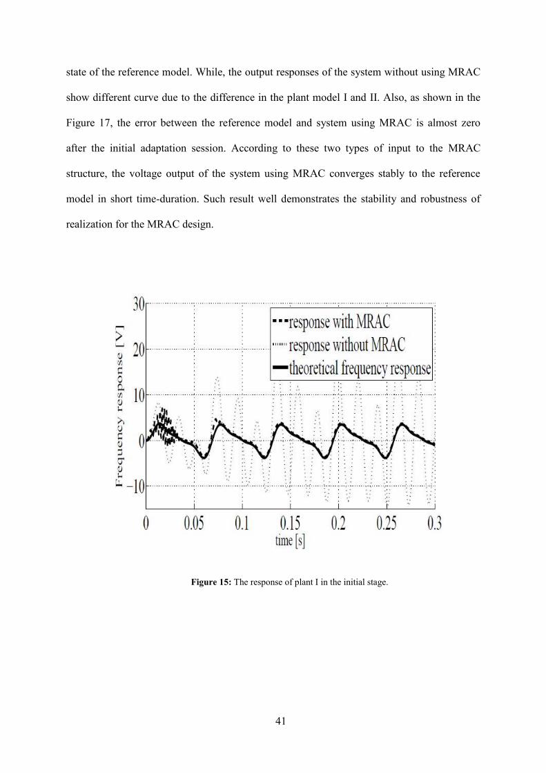
41

state of the reference model. While, the output responses of the system without using MRAC

show different curve due to the difference in the plant model I and II. Also, as shown in the

Figure 17, the error between the reference model and system using MRAC is almost zero

after the initial adaptation session. According to these two types of input to the MRAC

structure, the voltage output of the system using MRAC converges stably to the reference

model in short time-duration. Such result well demonstrates the stability and robustness of

realization for the MRAC design.

Figure 15: The response of plant I in the initial stage.

42

Figure 16: The response of plant II in the initial stage.

Figure 17: The error comparison of the sinusoidal input.

43

Last but not the least; it is instructive to know that one essential assumption in

designing this MRAC controller is this MRAC design is independent of the external

perturbance consideration. One reason is that it is hard to measure and model the noise or

disturbance of the photovoltaic power conversion system in the experiment with so many

constrains. In additional, assuming the model of perturbance is known, it will significantly

make the MRAC system complex enough to maintain the robust performance of the MRAC

control design and it will be overwhelming in the realization. The second reason is that under

the condition of modeling perturbance source, the photovoltaic system's convergence

performance with those obtained adaptive laws will not be asymptotically stable in the sense

of Lyapunov. Therefore, the future work in the MRAC designing improvement will mainly

mitigate the effect of perturbance in the system.

Given those simulation results obtained above, several conclusions about the MRAC

algorithm could be drawn. Firstly, the convergence rate of MRAC system could be obtained

extremely fast, being within one second, which is trivial enough to be noticed in the real

application. Secondly, no matter how the solar insolation and temperature changes, in term of

the plant description: the constantly changing damping ratio of the transfer function, MRAC

algorithm is always capable of tuning the plant model within a very short time, regardless of

the value of resistor. Having proven the stability and robustness of the MRAC algorithm from

the series of straightforward illustrations, another proof is tested to compare the controller

parameter from the actual simulation and the ideally calculation. By comparing the nominal

controller parameter and the practical controller parameter, it can mathematically prove the

asymptotically convergence is valid. The comparison between the nominal controller's

parameters and the updated controller's parameters is shown in Table 2. As shown in the

table, a reasonable agreement is obtained thereby demonstrating that the controller will

44

converge to the optimal power point. Based on the assumption of the plant that is monic

Hurwitz polynomial, the transfer function of the plant, after adaption, will still be a second-

order system. This is because the zero-pole cancellation takes place within the open left-hand

side of the s-plane.

Table 2: Comparison between the nominal and actual controller parameters

Nominal controller parameters for plant I -5.8 6.315 -0.515 1

Updated controller parameters for plant I -5.8 6.287 -0.500 1

Nominal controller parameters for plant II -5.94 6.56 -0.6204 1

Updated controller parameters for plant II -5.94 6.04 -0.6239 1

45

5.0 CONCLUSION AND FUTURE WORK

In order to improve the efficiency of photovoltaic systems, MPPT control algorithms

are used to optimize the power output of the systems. The essential considerations are the

accuracy and convergence time. As the simulation result extensively discussed in Section 4,

the statement that the proposed control system, by coupling two control algorithms, optimizes

the performance of the solution to the maximum power point tracking is convincing. As

reported in the literature, the duty cycle is obtained faster through the RCC method, which is

in the unit of millisecond. In the MRAC control system, the time constant of converging to

the characteristic of the reference model is couple of seconds and it is longer, compared to the

time constant of RCC. By tuning the adaptive gain in the adaptive law, the time constant can

be modulated to guarantee the stability of the entire system. By simulating the system

through different types of inputs, the proposed control system is sufficient robust and stable

to endure the small perturbance in the input and the measurements.

In the future work, related optimization work for this control system is mainly on two

aspects. Firstly, the RCC algorithm can be improved from the view of simple

implementation. As reported in the literature, the control law is not reliable enough to sustain

the perturbance of the noise. Proposing an alternative control law is plausible. Secondly, the

MRAC algorithm can be further well-designed with the consideration of the model of

perturbance, so that the performance of the MRAC can be enough robust. Thirdly, by

implementing the RCC algorithm in the simulation environment or the actual hardware

46

realization, the entire proposed control system can be simulated to test the performance of the

system.

47

APPENDIX A

MRAC CODING IN THE SIMULATION

function [ ky1h,ky2h,krh] = mrac( input,refnum,refden,ky1,ky2,kr ) ky1hat=10; ky2hat=10; kr=10; bm=refnum(1,1); am1=refden(1,2); am2=refden(1,3); ap1=-(ky1hat+ky2hat); ap2=ky1hat*ky2hat; bp=(ap2*bm)/(am2); plantnum=[bp]; plantden=[1,am1,am2]; t=[0:0.1:10]; r=10; for j=1:10 yp=step(plantnum,plantden,t); ym=step(refnum,refden,t); dyp=yp(2:length(yp))-yp(1:length(yp)-1); dym=ym(2:length(ym))-ym(1:length(ym)-1); temp1=(dyp-dym).*(dyp); temp2=(dyp-dym).*(yp(1:length(yp))); temp3=(dyp-dym)*(input).*(t(1:length(t)-1)); ky1h=-r*(bp)*(sum(temp1)); ky2h=-r*(bp)*(sum(temp2)); krh=-r*(bp)*(sum(temp3)); resulttemp=[ky1h,ky2h,krh]; end end

48

APPENDIX B

DATA COMPARISON CODING

function mraccompfirst load('error'); load('error1'); load('plantwithmrac'); load('reference'); load('plantwithoutmrac'); ref=referencemodel(2,:); plantwithmrac=pwith(2,:); plantwithoutmrac=pwithout(2,:); errortwo=error1(2,:); t=[40/400001:40/400001:40]; errorone=error(2,:); figure; hold on; %plot(t,errorone); %plot(t,errortwo); plot(t,plantwithmrac); plot(t,plantwithoutmrac); plot(t,ref); grid on; xlabel('time(s)'); ylabel('the error');

49

BIBLIOGRAPHY

[1]. Femia, N., et al., Optimization of perturb and observe maximum power point tracking

method. Power Electronics, IEEE Transactions on, 2005. 20(4): p. 963-973. [2]. Brunton, S.L., et al., Maximum power point tracking for photovoltaic optimization

using ripple-based extremum seeking control. Power Electronics, IEEE Transactions on, 2010. 25(10): p. 2531-2540.

[3]. Esram, T., et al., Dynamic maximum power point tracking of photovoltaic arrays

using ripple correlation control. Power Electronics, IEEE Transactions on, 2006. 21(5): p. 1282-1291.

[4]. Abdelsalam, A.K., et al., High-performance adaptive perturb and observe MPPT

technique for photovoltaic-based microgrids. Power Electronics, IEEE Transactions on, 2011. 26(4): p. 1010-1021.

[5]. Masoum, M.A.S., H. Dehbonei, and E.F. Fuchs, Theoretical and experimental

analyses of photovoltaic systems with voltageand current-based maximum power-

point tracking. Energy conversion, IEEE transactions on, 2002. 17(4): p. 514-522. [6]. Esram, T. and P.L. Chapman, Comparison of photovoltaic array maximum power

point tracking techniques. Energy conversion, IEEE transactions on, 2007. 22(2): p. 439-449.

[7]. Veerachary, M., T. Senjyu, and K. Uezato, Neural-network-based maximum-power-

point tracking of coupled-inductor interleaved-boost-converter-supplied PV system

using fuzzy controller. Industrial Electronics, IEEE Transactions on, 2003. 50(4): p. 749-758.

[8]. Kimball, J.W. and P.T. Krein, Discrete-time ripple correlation control for maximum

power point tracking. Power Electronics, IEEE Transactions on, 2008. 23(5): p. 2353-2362.

[9]. Krein, P.T. Ripple correlation control, with some applications. in Circuits and

Systems, 1999. ISCAS'99. Proceedings of the 1999 IEEE International Symposium on. 1999. IEEE.

[10]. Logue, D. and P. Krein. Optimization of power electronic systems using ripple

correlation control: a dynamic programming approach. in Power Electronics

Specialists Conference, 2001. PESC. 2001 IEEE 32nd Annual. 2001. IEEE.

50

[11]. Ioannou, P.A., Adaptive systems with reduced models. Lecture Notes in Control and

Information Sciences, 1983. [12]. Miller, D.E., A new approach to model reference adaptive control. Automatic

Control, IEEE Transactions on, 2003. 48(5): p. 743-757. [13]. Narendra, K. and L. Valavani, Stable adaptive controller design--Direct control.

Automatic Control, IEEE Transactions on, 1978. 23(4): p. 570-583. [14]. Narendra, K.S. and A.M. Annaswamy, Stable adaptive systems. 2005: Dover

Publications. [15]. Narendra, K.S. and P. Kudva, Stable adaptive schemes for system identification and

control-part I. Systems, Man and Cybernetics, IEEE Transactions on, 1974(6): p. 542-551.

[16]. Sastry, S. and M. Bodson, Adaptive control: stability, convergence and robustness.

2011: Dover Publications. [17]. Solodovnik, E.V., S. Liu, and R.A. Dougal, Power controller design for maximum

power tracking in solar installations. Power Electronics, IEEE Transactions on, 2004. 19(5): p. 1295-1304.

[18]. Jain, S. and V. Agarwal, A new algorithm for rapid tracking of approximate maximum

power point in photovoltaic systems. Power Electronics Letters, IEEE, 2004. 2(1): p. 16-19.