Joumal of Glaciology, Vol. 33, No. 113, 1987

MICRO-METEOROLOGICAL CONDITIONS FOR SNOW MELT

By M. KUHN

(Institut fiir Meteoroiogie und Geophysik, Universitat Innsbruck, A-6020 Innsbruck, Austria)

ABSTRACT. The energy budget of a snow or ice surface is determined by atmospheric variables like solar and atmospheric long-wave radiation, air temperature, and humidity; the transfer of energy from the free atmosphere to the surface depends on the stability of the atmospheric boundary layer, where vertical profiles of wind speed and temperature determine stability, and on surface conditions like surface temperature (and thus surface humidity), roughness, and albedo.

This paper investigates the conditions exactly at the onset or the end of melting using air temperature, humidity, and as the radiation term the sum of global and reflected short-wave plus downward long-wave radiation. For the turbulent exchange in the boundary la~'er, examples are computed with a transfer coefficient of 18.5 W m-2 K-1

which corresponds to the average over the ablation period on an Alpine glacier. Ways to estimate the transfer coefficient for various degrees of stability are indicated in the Appendix.

It appears from such calculations that snow may melt at air temperatures as low as -10 ° C and may stay frozen at +IO°C.

I. INTRODUCTION

The fact that snow melts at a temperature of Ts = o °c has often lead to the simplified assumption that it also melts at air temperatures of Ta = 0

0 C. This statement dis­

regards the intricacies of the energy budget of the snow surface in which radiation fluxes and turbulent exchange of latent heat operate independently of air temperature. In the following, a formulation is derived that permits the assess­ment of the meteorological conditions for snow melt in terms of absorbed radiation, humidity, and temperature of the atmospheric boundary layer above the snow surface.

The treatment of the problem is essentially an exercise in micro-meteorology. The partition of the energy budget obeys the conservation of energy law and is formally straightforward. Its application to real snow, however, is complicated by three facts:

(i) The separate variables chosen to describe a particular situation are not entirely independent, for instance, the atmospheric vapor density Pva is limited by air temperature Ta' and the long-wave downward radiation flux L l is to a certain degree coupled to Ta and pva· Such interconnections need to be considered when specifying a particular set of variables and will be explicitly stated in two examples in the text.

(ii) Because of the diurnal variation of the energy fluxes, stationarity is only approximated.

(iii) The transfer of heat through a turbulent boundary layer depends on external parameters such as wind speed and air temperature as well as internal ones like surface temperature and surface roughness.

In view of these complications, an a priori determination of the transfer coefficient is not attempted here. A value of 18.5 W m-2 K- I , as found from long-term observations on Alpine firn and ice (Kuhn, 1979), was used

24

10

o

-10

-20 o 2 4 6 8

* Pva

-3 Pva,g m

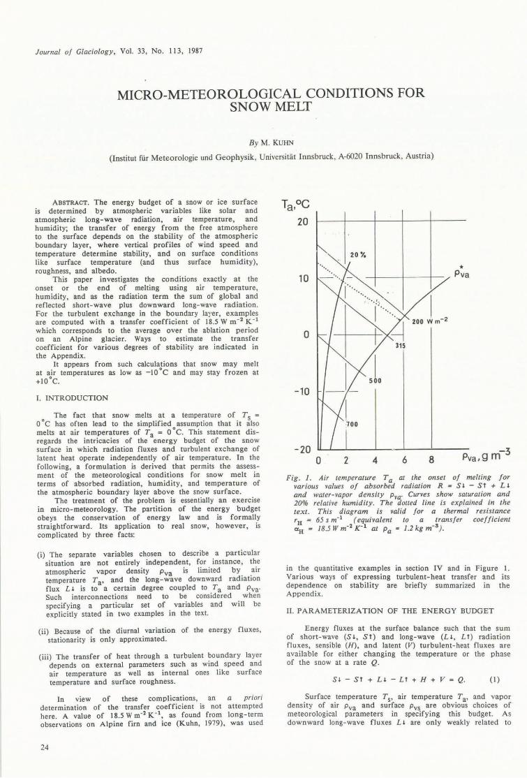
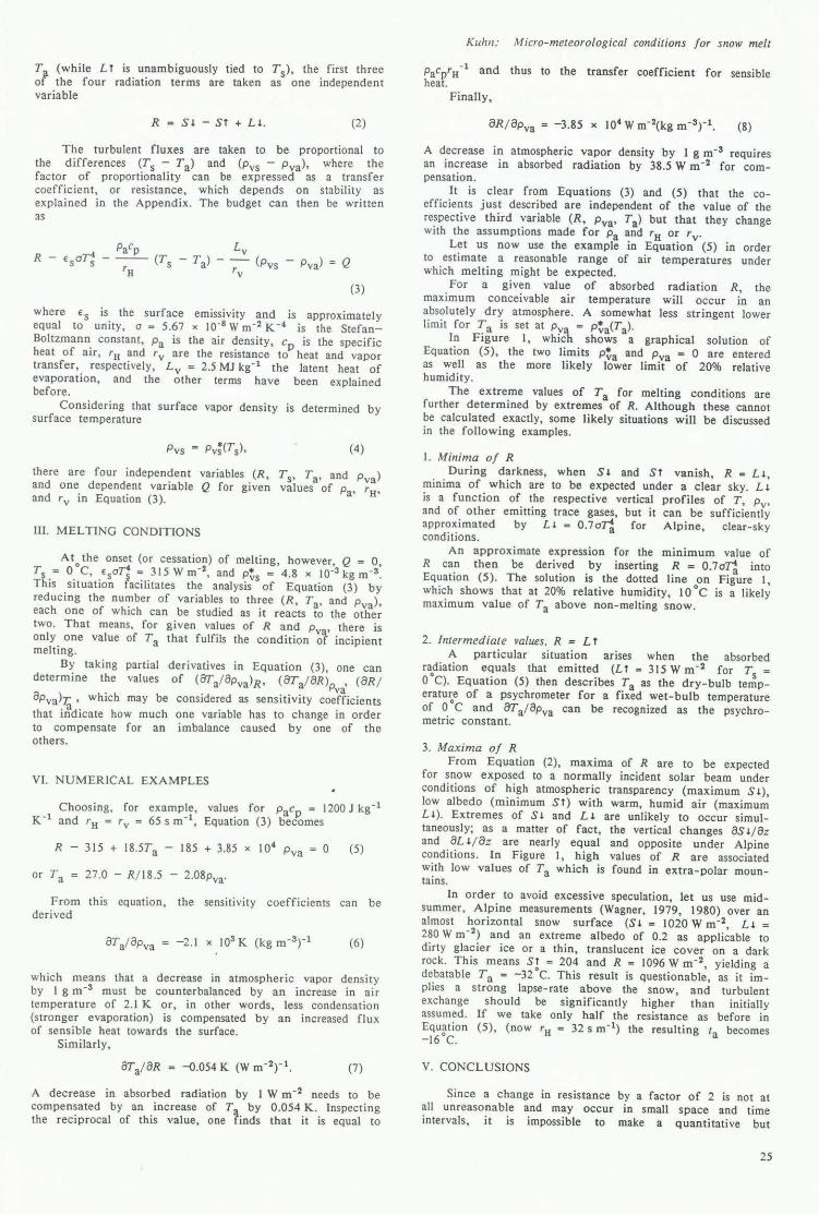
Fig. 1. Air temperature Ta at the onset of melting for various values of absorbed radiation R = S l - Sf + L l and water-vapor density pva. Curves show saturation and 20% relative humidity. The dotted line is explained in the text. This diagram is valid for a thermal resistance rH = 65 s m-I (equivalent to a transfer coefficient aH = 18.5 W m-2 rl at Pa = 1.2 kg m-s).

in the quantitative examples in section IV and in Figure I. Various ways of expressing turbulent-heat transfer and its dependence on stability are briefly summarized in the Appendix.

n. PARAMETERIZATION OF THE ENERGY BUDGET

Energy f1uxes at the surface balance such that the sum of short-wave (S l, Sf) and long-wave (L l, Lt) radiation fluxes, sensible (H), and latent (V) turbulent-heat fluxes are available for either changing the temperature or the phase of the snow at a rate Q.

Sl - St + Ll - Lt + H + V = Q. (I)

.Surface .temperature Ts' air temperature Ta' and vapor denSIty of aIr Pva and surface Pvs are obvious choices of meteorological parameters in specifying this budget. As downward long-wave f1uxes L l are only weakly related to

Ta (while L f is unambiguously tied to T s)' the first three of the four radiation terms are taken as one independent variable

R = S 1 - Sf + L 1. (2)

The turbulent fluxes are taken to be proportional to the d iff erences (Ts - Ta) and (Pvs - Pva)' where the factor of proportionality can be expressed as a transfer coefficient, or resistance, which depends on stability as explained in the Appendix. The budget can then be written as

Q 'v

(3)

where ES is the surface emissivity and is approximately equal to unity, 0 = 5.67 x 10-8 W m- 2 K -4 is the Stefan­Boltzmann constant, Pa is the air density, c is the specific heat of air, 'H and 'v are the resistance toP heat and vapor transfer, respectively, Lv = 2.5 MJ kg-! the latent heat of evaporation, and the other terms have been explained before.

Considering that surface vapor density is determined by surface temperature

(4)

there are four independent variables (R, Ts' Ta' and Pva) and one dependent variable Q for given values of Pa, 'H' and 'v in Equation (3).

Ill . MELTING CONDITIONS

Ato

the onset (or cessation) of melting, however, Q = 0, Ts.= O. C, .EsoT: ~ .315 W m-2

, and ~~s = 4.8 x 10-3 kg m- 3.

ThIs sItuatIOn faclhtates the analysIs of Equation (3) by reducing the number of variables to three (R, Ta' and Pva)' each one of which can be studied as it reacts to the other two. That means, for given values of Rand Pv ' there is only one value of Ta that fulfils the condition 01 incipient melting.

By taking partial determine the values

derivatives in Equation (3), one can of (BTa/BPva)R' (BTa/BR)p , (BRI

va BPva)I;;' which may be considered as sensitivity coefficients that indicate how much one variable has to change in order to compensate for an imbalance caused by one of the others.

VI. NUMERICAL EXAMPLES

Choosing, for example, values for Pacp = 1200 J kg-! K - l and rH = 'v = 65 s m-I, Equation (3) becomes

R 315 + 18 .5Ta - 185 + 3.85 x 104 Pva = 0 (5)

or Ta 27 .0 - R118.5 - 2.08pva '

From this equation, the sensitivity coefficients can be derived

which means that a decrease in atmospheric vapor density by I g m-3 must be counterbalanced by an increase in air temperature of 2. I K or, in other words, less condensation (stronger evaporation) is compensated by an increased flu x of sensible heat towards the surface .

Similarly,

(7)

A decrease in absorbed radiation by 1 W m- 2 needs to be compensated by an increase of T by 0.054 K. Inspecting the reciprocal of this value, one 1inds that it is equal to

Kuhll: Micro-meteorological conditions fo, snow melt

PaCp'H- l and thus to the transfer coefficient for sensible heat.

Finally,

(8)

A decrease in atmospheric vapor density by I g m-3 requires an increase in absorbed radiation by 38.5 W m -2 for com­pensation.

It is clear from Equations (3) and (5) that the co­efficients just described are independent of the value of the respective third variable (R, Pva' Ta) but that they change with the assumptions made for Pa and 'H or r v'

Let us now use the example in Equation (5) in order to estimate a reasonable range of air temperatures under which melting might be expected.

For a given value of absorbed radiation R, the maximum conceivable air temperature wiII occur in an absolutely dry atmosphere. A somewhat less stringent lower limit for Ta is set at Pva = p~a(Ta)'

In Figure I, which shows a graphical solution of Equation (5), the two limits P~a and Pva = 0 are entered as weII as the more likely lower limit of 20% relative humidity.

The extreme values of Ta for melting conditions are further determined by extremes of R. Although these cannot be calculated exactly, some likely situations wiII be discussed in the foIIowing examples.

1. Minima of R During darkness, when S 1 and Sf vanish, R = L 1,

minima of which are to be expected under a clear sky. L 1

is a function of the respective vertical profiles of T, PV '

and of other emitting trace gases, but it can be sufficiently approximated by L1 = 0.7071 for Alpine, clear-sky conditions.

An approximate expression for the minimum value of R can then be derived by inserting R = 0.7071 into Equation (5). The solution is the dotted line on Figure 1, which shows that at 20% relative humidity, JO ° C is a likely maximum value of Ta above non-melting snow.

2. Intermediate values. R = Lt A particular situation arises when the absorbed

radiation equals that emitted (L f = 3 I 5 W m -2 for T = O°C). Equation (5) then describes Ta as the dry-bulb te~p­erature of a psychrometer for a fixed wet-bulb temperature of 0 ° C and BT al Bpva can be recognized as the psychro­metric constant.

3. Maxima of R From Equation (2), maxima of R are to be expected

for snow exposed to a normaIIy incident solar beam under conditions of high atmospheric transparency (maximum S 1), low albedo (minimum Sf) with warm, humid air (maximum L 1) . Extremes of S 1 and L L are unlikely to occur simul­taneously; as a matter of fact, the vertical changes BS 11 Bz and BL1 / Bz are nearly equal and opposite under Alpine conditions. In Figure I, high values of R are associated with low values of Ta which is found in extra-polar moun­tains.

In order to avoid excessive speculation, let us use mid­summer, Alpine measurements (Wagner, 1979, 1980) over an almost horizontal snow surface (S 1 = 1020 W m -2 L 1 =

280 W m- 2 ) and an extreme albedo of 0.2 as appli~able to dirty glacier ice or a thin, translucent ice cover on a dark rock. This means S! = 204 and R = 1096 W m -2, yielding a debatable Ta = -32 C. This result is questionable, as it im­plies a strong lapse-rate above the snow, and turbulent exchange should be significantly higher than initially assumed. If we take only half the resistance as before in Equation (5), (now rH = 32 s m-I) the resulting t becomes -160C. a

V. CONCLUSIONS

Since a change in resistance by a factor of 2 is not at all unreasonable and may occur in smaII space and time intervals, it is impossible to make a quantitative but

25

Journal of Glaciology

generally true statement about the upper and lower limits of Ta' except, maybe, that the range _10° < Ta < +lO°C is likely to be encountered above snow at the beginning or end of melting (Q = 0).

Figure I treats both stable (Ta> O°C) and unstable situations with the same heat-transfer resistance but it is not intended to suggest that rH might be a constant for snow. To predict a value of rH' a number of micro­meteorological hypotheses need to be resolved and values of Ta' u, u. ' and Zo need to be known, as described in the Appendix. However, for c1imatological applications of the present problem, the range of rH is small and likely to be centered around the value of 65 s m-I found in the ablation period of an Alpine glacier.

Considering that the determination of rH is a crucial problem in calculating the energy budget, we may even venture to use a form of Equation (3) to determine rH = r v from measurements of R, Ta' and Pva at a time when Q = 0

rH = rv = Pacpll.T + Lvll.pv

R - 315 (9)

taking care that R is sufficiently different from 315 W m- 2 .

REFERENCES

Brutsaert, W. 1982. Evaporation into the atmosphere. Dordrecht, Reidel.

Bush, N .E. 1973. The surface boundary layer (Part I). Boundary Layer Meteorology, Vol. 4, p. 213-40.

Carson, 0 .1., and Richards, P.l.R. 1978. Modelling surface turbulent fluxes in stable conditions. Boundary Layer Meteorology, Vol. 14, p. 67-81.

Kuhn, M. 1979. On the computation of heat transfer coefficients from energy-balance gradients on a glacier. Journal of Glaciology, Vol. 22, No. 87, p. 263-72.

Wagner, H.P. 1979. Strahlungshaushaltsuntersuchungen an einem Ostalpengletscher wlihrend der Hauptablationsperiode. Teil I: Kurzwellige Strahlung. Archiv fur Meteorologie , Geophysik und Bioklimatologie, Ser. B, Bd. 27, p. 297-324.

Wagner, H.P. 1980. Strahlungshaushaltsuntersuchungen an einem Ostalpengletscher wlihrend der Hauptablationsperiode. Teil 2: Langwellige Strahlung und Strahlungsbilanz. Archiv fur Meteorologie , Geophysik und Bioklimatologie, Ser. B, Bd. 28, p. 41-62.

APPENDIX

The turbulent fluxes of sensible heat H and of latent heat V are defined here as positive when energy flows to the surface. According to the gradient hypothesis, they can be expressed

With

and neglecting g/cp « aT/az,

-1 aT H = PaCpKU. ~H -a- and V

Inz

(A.I)

(A.2)

L KU 41 -1~ V • v alnz

The desired form with finite differences and a bulk transfer number

is obtained by integration of Equations (A.3) from the surface (zo) to the level of measurements.

and

z V f ~vd(lnz) = Lv KU.(pva(z) - pvs )'

Zo

(A.5)

Comparison of Equations (AA) with Equations (A.5) yields

(A.6)

and with ~v

(A .7)

which can be expressed as a function of wind speed by inserting for u. from the logarithmic wind profile

z u(z) = K-

1U. J ~Md(1nz) (A .8)

Zo

where ~M is the stability function for momentum flux . The function 41 was determined from experiments as re­

viewed by Brutsaert (1982), Bush (1973) or Carson and Richards ('1978), among others. The simplest expression holds for stable layering where

and a = 5, approximately. The Monin-Dbukhov length is

L* (A.10) KgH(1 + 0.07H/ V)

using the notation and sign convention of this paper. The stability functions may also be expressed in terms

of the Gradient-Richardson number Ri

Ri g (aT/Bz + g/cp)(l + 0.007H/V)

T (Bu/az) 2

~ ~ _aT~/....:a-=z"... T (au/ az)2'

(A.II)

Under stable conditions (~M = 4lH)

Ri (A.12)

(A.3) from which a useful approximation can be derived with a = 5

where K is the von Karman constant, u. is the friction velocity , and ~ is a function of stability.

MS. received 1 October 1986

26

4lM (I - 5Rir1 '" 1 + 5Ri. (A.13)