Embed Size (px)
Citation preview

arX
iv:0
911.
3787
v1 [
mat
h.ST
] 1
9 N
ov 2
009
The Annals of Statistics
2009, Vol. 37, No. 6B, 4011–4045DOI: 10.1214/09-AOS704c© Institute of Mathematical Statistics, 2009
TESTING CONDITIONAL INDEPENDENCE VIAROSENBLATT TRANSFORMS
By Kyungchul Song
University of Pennsylvania
This paper proposes new tests of conditional independence of tworandom variables given a single-index involving an unknown finite-dimensional parameter. The tests employ Rosenblatt transforms andare shown to be distribution-free while retaining computational con-venience. Some results from Monte Carlo simulations are presentedand discussed.
1. Introduction. Suppose that Y and Z are random variables, and letλθ(X) be a real function of a random vector X indexed by a parameterθ ∈ Θ ⊂ R
d. The function λθ(·) is known up to θ ∈ Θ. For example, wemay consider λθ(X) = h(X⊤θ) for some known function h. Suppose that anestimable parameter θ0 ∈Θ is given. This paper proposes a distribution-freemethod of testing conditional independence of Y and Z given λθ0(X),
Y ⊥⊥ Z|λθ0(X).(1)
When Y and Z are conditionally independent given λθ0(X), it means that“learning the value of Z does not provide additional information about Y ,once we know λθ0(X)” [Pearl (2000), page 11]. Hence conditional indepen-dence is a central notion in modeling causal relations, and its importance ingraphical modeling is widely known [e.g., Lauritzen (1996), Pearl (2000)]. Inthe literature of program evaluations, testing conditional independence ofthe observed outcome and the treatment decision given observed covariatescan serve as testing lack of treatment effects under the assumption of strongignorability [Heckman, Ichimura and Todd (1997)]. Conditional indepen-dence is, sometimes, a direct implication of economic theory. For example,in the literature of insurance, the presence of positive conditional depen-dence between coverage and risk is known to be a direct consequence of
Received January 2009; revised April 2009.AMS 2000 subject classifications. 62G07, 62G09, 62G10.Key words and phrases. Conditional independence, distribution-free tests, Rosenblatt
transforms, wild bootstrap.
This is an electronic reprint of the original article published by theInstitute of Mathematical Statistics in The Annals of Statistics,2009, Vol. 37, No. 6B, 4011–4045. This reprint differs from the original inpagination and typographic detail.
1

2 K. SONG
adverse selection under information asymmetry [e.g., Chiappori and Salanie(2000)].
Testing independence for continuous variables has drawn the attention ofmany researchers. To name but a few, see Hoeffding (1948), Blum, Kieferand Rosenblatt (1961), Skaug and Tjøstheim (1993), Robinson (1991), Del-gado and Mora (2000) and Hong and White (2005). There has also beena growth of interest in testing extremal dependence. See a recent paperby Zhang (2008) and references therein. In contrast, the literature of test-ing conditional independence for continuous variables appears rather recentand includes relatively few researches. See Linton and Gozalo (1997), Del-gado and Gonzalez Manteiga (2001), Angrist and Kuersteiner (2004) andSu and White (2008), among others. None of these tests focuses on condi-tional independence between continuous variables with unknown θ0 and isdistribution-free at the same time.
Distribution-free tests have asymptotic critical values that do not changeas we move from one probability to another within the null hypothesis.Many goodness-of-fit tests that have nontrivial asymptotic power against√
n-converging Pitman local alternatives are not distribution-free. To dealwith this problem, the literature either suggests the use of approximatecritical values through bootstrap or the transformation of the test using theinnovation martingale approach pioneered by Khmaladze (1993).
This paper shows that for testing conditional independence, we can gener-ate distribution-free tests by appropriately using Rosenblatt transforms—amultivariate version of a probability integral transform studied by Rosen-blatt (1952). Based on the result, this paper proposes a bootstrap methodthat is computationally attractive. This bootstrap procedure does not re-quire the re-estimation of θ0 for each bootstrap sample. This is convenientwhen the dimension of θ0 is large and its estimation involves numerical op-timization.
The Rosenblatt transform is closely related to the probability integraltransform of a single-index suggested by Stute and Zhu (2005). However, thenature of the problem is distinguished from that of Stute and Zhu (2005).First, our test of conditional independence is both omnibus (when the testis two-sided) and distribution-free, while the single-index restriction test ofStute and Zhu (2005) fails to be distribution-free when it is designed to beomnibus. This is purely due to the nature of conditional independence asdistinct from a single-index restriction. Second, our test contains the proba-bility integral transform inside functions that are potentially discontinuous,making it cumbersome to rely on the U -process theory [e.g., de la Pena andGine (1999)]. This paper deals with this difficulty by directly establishing thebracketing entropy bounds for functions involving the probability integraltransforms. These entropy bounds can be used for other purposes.
TESTING CONDITIONAL INDEPENDENCE 3
This paper is organized as follows. In the next section, we introduce thebasic assumptions and test statistics, and develop asymptotic theory. InSection 3, we consider a bootstrap method. Section 4 deals with the casewhere Z is discrete. In Section 5, we present and discuss the results from theMonte Carlo simulation study. In the Appendix, we offer the mathematicalproofs.
2. Main results. Suppose that we are given a random vector (Y,Z,X)distributed by P and a real valued function λθ0(·) on R
dX which is knownup to a parameter θ0 ∈ Θ ⊂ R
d. For brevity, let λ0(·) ≡ λθ0(·). Throughoutthis paper, we assume that λ0(X) is continuous. Define F0(·) to be thedistribution function of λ0(X) and let U ≡ F0(λ0(X)), FY |U (·|U) ≡ P{Y ≤·|U}, and FZ|U(·|U) ≡ P{Z ≤ ·|U}. Then, the main focus of this paper is ontesting the following hypothesis:
H0 :P{Y ≤ y,Z ≤ z|U} = FY |U (y|U)FZ|U (z|U) wp 1,(2)
for all (y, z) in the support of (Y,Z). The notation “wp 1” means that thestatement holds with probability one with respect to the distribution of U .Certainly, this hypothesis is equivalent to (1) with probability one becauseF0(·) is continuous.
Throughout the paper, the norm ‖ · ‖∞ represents the sup norm, ‖ · ‖, theEuclidean norm and ‖ · ‖P,p, the Lp(P )-norm. Let B(θ0, δ) ≡ {θ ∈ Θ:‖θ −θ0‖ ≤ δ}. Define
Y ≡ FY |U(Y |U) and Z ≡ FZ|U(Z|U),
then (Z,U) is distributed as the joint distribution of two independent uni-form [0,1] random variables, and so is (Y ,U), if (Z,λ0(X)) and (Y,λ0(X))are continuous [Rosenblatt (1952)]. The transform of (Z,λ0(X)) into (Z,U)is called the Rosenblatt transform, due to Rosenblatt (1952). Let fY |Z,θ(y|z,
λ1, λ0) be the conditional density of Y given (Z, λθ(X), λ0(X)) = (z, λ1, λ0)with respect to a σ-finite conditional measure. We also define fZ|Y,θ(z|y, λ1, λ0)
similarly by interchanging the roles of Y and Z.
Assumption 1. (i) (Y,Z,λ0(X)) is continuous.(ii) For some δ > 0,
(a) λθ(·), θ ∈ B(θ0, δ), is uniformly bounded and Lipschitz in θ, thatis, for any θ1, θ2 ∈B(θ0, δ),
‖λθ1 − λθ2‖∞ ≤C‖θ1 − θ2‖ for some C > 0 and
(b) λθ(X) is continuous, having a density function bounded uni-formly over θ ∈ B(θ0, δ).

4 K. SONG
(iii) For some δ > 0, fZ|Y,θ(z|y, ·, λ0) and fY |Z,θ(y|z, ·, λ0) are continuously
differentiable with derivatives bounded uniformly over (y, z, λ0, θ)∈ [0,1]2 ×R×B(θ0, δ).
Later in the paper (Section 4), we deal with the case where either Yor Z is discrete. The uniform boundedness condition in (ii) is innocuous,because by choosing a strictly increasing function Φ on [0,1], we can redefineλ′
θ = Φ ◦ λθ. The Lipschitz continuity in θ can be made to hold by choosingthis Φ appropriately. The absolute continuity condition in (ii)(b) is satisfiedin particular when λθ(X) = h(X⊤θ) with a continuous, strictly increasingfunction h and X⊤θ is continuous.
Define
γz(·) ≡ z exp(· × z) and γ⊥z (·) ≡ γz(·)−{exp(z)− 1}.
For a class of functions βu(·), u ∈ [0,1], consider the following null hypoth-esis:
H0 :E[βu(U)γ⊥z (Z)γ⊥
y (Y )] = 0 ∀(u, y, z) ∈ [0,1]3.(3)
The lemma below establishes that under Assumption 1(i), and an appropri-ate condition for βu, the null hypothesis in (2) and the null hypothesis in(3) are equivalent. The result relies on Lemma 1 of Bierens (1990).
Lemma 1. Suppose that Assumption 1(i) is satisfied. Furthermore, as-sume that the class {βu, u ∈ [0,1]} is such that (3) implies the following:
E[γ⊥z (Z)γ⊥
y (Y )|U ] = 0 wp 1 ∀(y, z) ∈ [0,1]2.(4)
Then, the hypothesis in (2) and the hypothesis in (3) are equivalent.
Proof. It is easy to see that the conditional independence (2) implies(3). We prove the converse. First, we show that the conditional independenceof Y and Z given U implies (2). Suppose that this conditional independenceholds. Let y = FY |U(y|U) and z = FZ|U(z|U) for brevity. Write
P{Y ≤ y, Z ≤ z|U}= P{Y ≤ y, Z ≤ z, Y ≤ y,Z ≤ z|U}
+ P{Y ≤ y, Z ≤ z, Y > y,Z ≤ z|U}(5)
+ P{Y ≤ y, Z ≤ z, Y ≤ y,Z > z|U}+ P{Y ≤ y, Z ≤ z, Y > y,Z > z|U}.
Following Angus (1994), the second probability on the right-hand side isbounded by
P{Y ≤ y, Y > y|U} = P{Y = y, Y > y|U}= P{FY |U (Y |U) = FY |U (y|U), Y > y|U} = 0,

TESTING CONDITIONAL INDEPENDENCE 5
because conditional on U = u, the event in the last probability is containedin the event of Y lying in the interior of an interval of constancy of FY |U (·|u).The conditional probability measure of this event is certainly zero. Similarly,the last two probabilities in (5) can also be shown to be zero. If Y ≤ y andZ ≤ z, then Y ≤ y and Z ≤ z. Therefore, we obtain from (5) that
P{Y ≤ y,Z ≤ z|U} = P{Y ≤ y, Z ≤ z|U}.(6)
Using a similar argument, we can also obtain that
P{Y ≤ y|U} = P{Y ≤ y|U} = y and(7)
P{Z ≤ z|U} = P{Z ≤ z|U} = z,
because Y is uniformly distributed on [0,1] and independent of U , and sois Z . Conditional independence of Y and Z given U implies (2) through (6)and (7).
Now, we show that (3) implies conditional independence of Y and Z givenU . Let f(t1, t2|u) : [0,1]2 → [0,∞) be the conditional density of (Z, Y ) givenU = u. Through (4), (3) implies that for all (z, y) ∈ [0,1]2,
zy
∫ 1
0
∫ 1
0ezt1+yt2{f(t1, t2|U)− 1}dt1 dt2 = 0 wp 1.
By Lemma 1 of Bierens (1990) [see also Stinchcombe and White (1998), page4], f(t1, t2|U) = 1{(t1, t2) ∈ [0,1]2}, a.e., for almost every (t1, t2) ∈ [0,1]2,yielding conditional independence of Y and Z given U . �
The condition for βu(·) in Lemma 1 is explained in Stinchcombe andWhite (1998). For example, the choice of βu(U) = 1{U ≤ u} or βu(U) =exp(Uu) satisfies this condition [see Bierens (1990), Lemma 1, for the latterchoice]. From now on, we assume that βu(·) satisfies the condition in Lemma1 and focus on the null hypothesis in (3). This condition for βu(·) is not usedfor the weak convergence theory in Theorem 1 below.
Assumption 2. (i) βu(·), u ∈ [0,1], is uniformly bounded in [0,1], andfor each u ∈ [0,1], βu(·) is of bounded variation.
(ii) FY |U(y|·) and FZ|U (z|·) are twice continuously differentiable with
derivatives bounded uniformly over (z, y) ∈R2.
Assumption 2(i) is very weak and satisfied by most functions used in theliterature. This flexibility in choosing the class βu is important because thechoice of βu plays a significant role in determining the asymptotic powerproperties of the test in general. Assumption 2(ii) is analogous to ConditionA(i) in Theorem 2.1 of Stute and Zhu (2005) or A2 of Delgado and GonzalezManteiga (2001) on page 1475.

6 K. SONG
Throughout this paper, we assume that the observations (Yi,Xi,Zi)ni=1
are i.i.d. from P . We also assume that the parameter θ0 is identified fromdata and estimable. For example, in the literature of program evaluations,this assumption is satisfied because the parameter θ0 constitutes the single-index in the propensity score. Let θ be a consistent estimator of θ0, anddefine
Ui ≡ Fn,θ,i(λθ(Xi)), Zi ≡ FZ|U,i(Zi|Ui) and Yi ≡ FY |U,i(Yi|Ui),
where Fn,θ,i(λ)≡ 1n−1
∑nj=1,j 6=i 1{λθ(Xj) ≤ λ}, and
FY |U,i(y|u)≡∑n
j=1,j 6=i 1{Yj ≤ y}Kh(Uj − u)∑n
j=1,j 6=i Kh(Uj − u),(8)
where Kh(x) = K(x/h)/h, K(·) is a kernel function and h is the bandwidth
parameter. We similarly define FZ|U,i(z|u). As for the estimator θ, the kerneland the bandwidth, we assume the following.
Assumption 3. (i) ‖θ − θ0‖= OP (n−1/2).(ii) (a) K is symmetric, nonnegative, twice continuously differentiable,
has a compact support, and∫∞−∞ K(s) = 1.
(b) h = Cn−s with 1/6 < s < 1/4 for some C > 0.
When θ is an M -estimator, the rate of convergence in (i) can be obtainedfollowing the procedure of Theorem 3.2.5 of van der Vaart and Wellner(1996). The estimation method of θ0 depends on a further specification ofthe testing environment. For example, the conditioning variable λθ(Xi) mayoriginate from the nonlinear regression model,
Wi = λθ0(Xi) + εi,
where εi satisfies E[εi|Xi] = 0. The√
n-consistent estimation of θ0 in thiscase is well known in the literature [see, e.g., van de Geer (2000)]. Assump-tion 3(ii)(a) is used by Stute and Zhu (2005). Unlike their procedure, thebandwidth condition in (b) does not require undersmoothing.
Define the infeasible and feasible processes
νn(r) ≡ 1√n
n∑
i=1
βu(Ui)γ⊥z (Zi)γ
⊥y (Yi)
and
νn(r)≡ 1√n
n∑
i=1
βu(Ui)γ⊥z (Zi)γ
⊥y (Yi).
In the following, we establish weak convergence of both processes. The maincomplication is that the condition for βu (Assumption 2) is too weak to resort

TESTING CONDITIONAL INDEPENDENCE 7
to linearization in handling the estimation error of Ui. We deal with thisdifficulty by establishing a bracketing entropy bound for functions compositewith bounded variation functions (see Lemma A1 in the Appendix). Letl∞([0,1]3) denote the space of real functions on [0,1]3 that are bounded,and endowed with a sup norm ‖ · ‖∞ defined by ‖f‖∞ = supu∈[0,1]3|f(u)|.The notation denotes weak convergence in l∞([0,1]3) in the sense ofHoffman–Jorgensen [e.g., van der Vaart and Wellner (1996)]. Let 〈·, ·〉 be
the inner product on L2(du)×L2(du) defined by 〈f, g〉=∫ 10 f(u)g(u)du.
Theorem 1. Suppose that Assumptions 1–3 hold. Then the followingholds:
(i) supr∈[0,1]3 |νn(r)−νn(r)|= oP (1), both under H0 in (3) and under Pit-
man local alternatives Pn such that for some functions aj : [0,1]3 → [−1,1],j = 1,2,
EPn[γ⊥
z (Z)|Y = y,U = u] = n−1/2a1(z, y, u)
and
EPn[γ⊥
y (Y )|Z = z,U = u] = n−1/2a2(z, y, u),
where EPn[·|Y = y,U = u] and EPn
[·|Z = z,U = u] denote conditional expec-
tations under Pn.(ii) νn ν in l∞([0,1]3), under H0 in (3), where ν is a centered Gaussian
process whose covariance kernel is given by
c(r1; r2) = 〈βu1 , βu2〉〈γ⊥z1
, γ⊥z2〉〈γ⊥
y1, γ⊥
y2〉.
The asymptotic representation in (i) shows an interesting fact that νn(r)
is asymptotically equivalent to νn(r). Remarkably, the estimation error in θdoes not play a role in shaping the asymptotic distribution of the processνn(r). This finding is analogous to what Stute and Zhu (2005) found in thecontext of testing a single-index restriction.
Based on the result in Theorem 1, we can construct a test statistic
Tn = Γνn(9)
by taking a continuous functional Γ. For example, in the case of two sidedtests, we may take
ΓKSνn = supr∈[0,1]3
|νn(r)| or ΓCMνn =
(∫
[0,1]3νn(r)2 dr
)1/2
.(10)
The first example is of Kolmogorov–Smirnov-type and the second one isof Cramer–von Mises-type. Asymptotic unbiasedness for these tests against

8 K. SONG
√n-converging local alternatives can be established using Anderson’s lemma.
In the case of one-sided tests, we may take
Γ+KSνn = sup
r∈[0,1]3νn(r) or Γ+
CMνn =
(∫
[0,1]3max{νn(r),0}2 dr
)1/2
.
The asymptotic properties of the tests follow from Theorem 1. Indeed, underH0,
Tn = Γνn →d Γν.(11)
This test is distribution-free, as the limiting distribution of Γν does notdepend on the data generating process under H0.
3. Bootstrap tests. The tests introduced so far are distribution-free, but,in many cases, it is not known how to simulate the Gaussian process ν. In thissection, we suggest a wild bootstrap method in a spirit similar to Delgadoand Gonzalez Manteiga (2001) [see also, among others, Hardle and Mammen(1993), Stute, Gonzalez Manteiga and Quindimil (1998)].
Let ({ωi,b}ni=1)
Bb=1 be an i.i.d. sequence of random variables that are
bounded, independent of {Yi,Zi,Xi}, E(ωi,b) = 0 and E(ω2i,b) = 1. For exam-
ple, one can take ωi,b with a two-point distribution assigning masses (√
5 +
1)/(2√
5) and (√
5 − 1)/(2√
5) to the points −(√
5 − 1)/2 and (√
5 + 1)/2.Let
ν∗n,b(r) =
1√n
n∑
i=1
ωi,bβu(Ui)γ⊥z (Zi)γ
⊥y (Yi), b = 1, . . . ,B.
The bootstrap empirical process ν∗n,b(r) is similar to those proposed by Del-
gado and Gonzalez Manteiga (2001). Given a functional Γ, we can definebootstrap test statistics T ∗
n,b = Γν∗n,b, b = 1, . . . ,B. An α-level critical value
is approximated by cα,n,B = inf{t :B−1ΣBb=11{T ∗
n,b ≤ t} ≥ 1 − α}, yieldingbootstrap test 1{Tn > cα,n,B}, where Tn is as defined in (9).
Let FΓν be the distribution of Γν and let F ∗T ∗
ndenote the conditional
distributions of bootstrap test statistics T ∗n . Define d(·, ·) to be a distance
metrizing weak convergence on the real line. [For an introductory exposi-tion about the weak convergence of bootstrap empirical processes, see Gine(1997)]. The weak convergence follows eventually as a consequence of thealmost sure multiplier CLT of Ledoux and Talagrand (1988).
Theorem 2. Suppose that the conditions of Theorem 1 hold under H0
in (3). Then under H0,
d(F ∗T ∗
n, FΓν)→ 0 in P.

TESTING CONDITIONAL INDEPENDENCE 9
The wild bootstrap procedure is easy to implement. In particular, one doesnot need to re-estimate θ0 or (Zi, Yi) using each bootstrap sample. It is worthnoting that this desirable property is made possible by our transforming thetest into a distribution-free one.
4. Discrete random variables. The development so far has assumed thatY and Z are continuous random variables. In many important applicationsof conditional independence, either Y or Z is discrete, or more often, binary.For example, in the literature of program evaluations, the conditional inde-pendence restriction involves a binary variable representing the incidence oftreatment.
From now on, we assume that Y is continuous and Z is discrete, takingvalues from a known, finite set Z . We introduce (Y ,U) as before. Definepz(U) = P{Z = z|U} for z ∈Z . Similarly as in Lemma 1, we can show thatthe null hypothesis in (2) is equivalent to
H0 :E[βu(U){1{Z = z} − pz(U)}γ⊥y (Y )] = 0 ∀(y,u, z) ∈ [0,1]2 ×Z,
if (Y,λ0(X)) is continuous and βu satisfies approximate conditions similarlyas in Lemma 1. We substitute the following for Assumption 1.
Assumption 1D. (i) (Y,λ0(X)) is continuous.(ii) Assumption 1(ii) holds for λθ, θ ∈Θ.(iii) For some δ > 0, fY |Z,θ(y|z, ·, λ0) is continuously differentiable with a
derivative bounded uniformly over (y, z, λ0, θ)∈ [0,1]×Z ×R×B(θ0, δ).(iv) For some ε > 0, pz(u) ∈ (ε,1− ε) for all (u, z) ∈ [0,1]×Z .
Let pz,i(u) be a kernel estimator of pz(u),
pz,i(u) =
∑nj=1,j 6=i 1{Zj = z}Kh(Uj − u)
∑nj=1 Kh(Uj − u)
(12)
and consider the following process: for (u, y, z) ∈ [0,1]2 ×Z ,
νn(u, y, z) ≡ 1√n
n∑
i=1
βu(Ui){1{Zi = z} − pz,i(Ui)}γ⊥y (Yi)
√
pz,i(Ui)− pz,i(Ui)2,
where Yi and Ui are as defined before.
Theorem 3. Suppose that Assumptions 1D, 2 and 3 hold. Furthermore,the conditions for K and h used for pz,i(·) are the same as Assumption 3(ii).Then under H0,
νn ν in l∞([0,1]2 ×Z),

10 K. SONG
where ν is a centered Gaussian process whose covariance kernel is given by
c(r1, r2)≡{
〈βu1 , βu2〉〈γ⊥y1
, γ⊥y2〉, if z1 = z2,
0, if z1 6= z2.
Theorem 3 shows that we can generate distribution-free tests based onνn. Test statistics are constructed using an appropriate functional Γ: forexample,
Γνn = sup(u,y,z)∈[0,1]2×Z
|νn(u, y, z)|
or
Γνn =
(
∑
z∈Z
∫
[0,1]2νn(u, y, z)2 d(u, y)
)1/2
.
When the Gaussian process ν can be simulated, asymptotic critical valuescan be read from the distribution of Γν. When this is not possible or difficult,one may consider the following bootstrap procedure. Take ωi,b as in Section4. Define the bootstrap process
ν∗n,b(u, y, z) ≡ 1√
n
n∑
i=1
ωi,bβu(Ui){1{Zi = z} − pz,i(Ui)}γ⊥y (Yi)
√
pz,i(Ui)− pz,i(Ui)2.
We construct the bootstrap test statistics T ∗n,b = Γν∗
n,b, b = 1, . . . ,B, using anappropriate functional Γ.
Theorem 4. Suppose that the conditions of Theorem 3 hold. Then underH0,
d(F ∗T ∗
n, FΓν)→ 0 in P.
5. Simulation studies.
5.1. Conditional independence between continuous variables. We sam-pled Xi as i.i.d. Unif[0,1] and Zi = aXi +(1−a)ηi, where ηi ∼ i.i.d.Unif[0,1]and a ∈ {0.2,0.5}.
We first consider the finite sample size properties of the bootstrap tests.For this purpose, Yi’s were generated as follows:
DGP A1: Yi = Φ((Xi − 0.5)/√
0.2) + εi,
DGP A2: Yi = sin(5Xi) + εi,
where εi ∼ N(0,1) and Φ denotes the standard normal c.d.f. All the DGPsallow Yi to depend on Zi, but only through Xi, and hence belong to the nullhypothesis. The DGPs admit different types of nonlinearity in Xi.

TESTING CONDITIONAL INDEPENDENCE 11
Table 1
Rejection probabilities under the null hypothesis of conditional independenceamong continuous variables
Exp. Ind.
DGP a h 1% 5% 10% 1% 5% 10%
A1 0.2 0.25× n−1/5 0.0140 0.0680 0.1285 0.0210 0.0715 0.1340
0.50× n−1/5 0.0125 0.0540 0.1165 0.0165 0.0615 0.1160
1.00× n−1/5 0.0120 0.0525 0.1100 0.0140 0.0585 0.1125
2.00× n−1/5 0.0115 0.0520 0.1090 0.0125 0.0570 0.1025
0.5 0.25× n−1/5 0.0225 0.0610 0.1180 0.0160 0.0695 0.1280
0.50× n−1/5 0.0140 0.0580 0.1090 0.0125 0.0540 0.1065
1.00× n−1/5 0.0105 0.0540 0.0965 0.0120 0.0455 0.1000
2.00× n−1/5 0.0195 0.0690 0.1315 0.0170 0.0650 0.1315
A2 0.2 0.25× n−1/5 0.0200 0.0645 0.1295 0.0155 0.0660 0.1215
0.50× n−1/5 0.0120 0.0555 0.1055 0.0100 0.0560 0.1130
1.00× n−1/5 0.0115 0.0500 0.1025 0.0100 0.0490 0.1000
2.00× n−1/5 0.0120 0.0495 0.1095 0.0130 0.0485 0.1040
0.5 0.25× n−1/5 0.0240 0.0765 0.1385 0.0185 0.0690 0.1295
0.50× n−1/5 0.0225 0.0640 0.1200 0.0135 0.0700 0.1155
1.00× n−1/5 0.0135 0.0635 0.1150 0.0165 0.0495 0.1035
2.00× n−1/5 0.0760 0.2185 0.3285 0.0225 0.0775 0.1465
We focus on two types of bootstrap-based tests: one with βu(U) = 1{U ≤u} (denoted “Ind.” in the tables) and the other with βu(U) = exp(Uu)(denoted “Exp.” in the tables). Nonparametric estimations in the Rosen-blatt transforms were done using kernel estimation with the kernel K(u) =
(15/16)(1−u2)21{|u| ≤ 1}. The bandwidths for Yi and Zi were chosen to bethe same, being equal to h = cn−1/5 with c ranging in {0.25,0.5,1,2}. In con-structing Kolmogorov–Smirnov tests, we used 103 equal-spaced grid pointsin [0,1]3. The bootstrap Monte Carlo simulation number and the MonteCarlo simulation number for the whole procedure were set to be 2000. Thesample size was equal to 100.
Finite sample sizes are reported in Table 1. The rejection probabilities areoverall stable over different choices of bandwidths for all the tests, althoughthey are slightly more sensitive to the bandwidth choices in the case of highercorrelation between Xi and Zi (corresponding to a = 0.5).
As for the power properties of the tests, we consider the following fourdata generating processes:
DGP B1: Yi = Φ((Xi − 0.5)/√
0.2) + Φ((Zi − 0.5)/√
0.2) + εi,
DGP B2: Yi = Φ((Xi − 0.5)/√
0.2) + sin(5Zi) + εi,
12 K. SONG
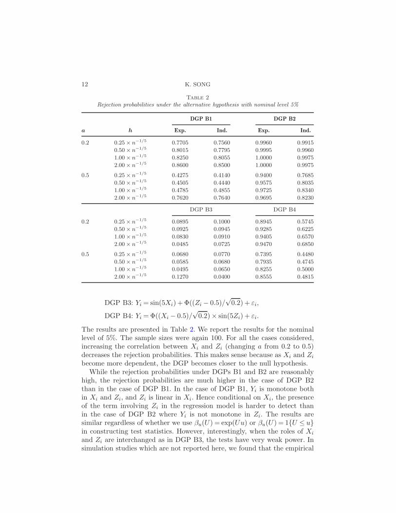
Table 2
Rejection probabilities under the alternative hypothesis with nominal level 5%
DGP B1 DGP B2
a h Exp. Ind. Exp. Ind.
0.2 0.25× n−1/5 0.7705 0.7560 0.9960 0.9915
0.50× n−1/5 0.8015 0.7795 0.9995 0.9960
1.00× n−1/5 0.8250 0.8055 1.0000 0.9975
2.00× n−1/5 0.8600 0.8500 1.0000 0.9975
0.5 0.25× n−1/5 0.4275 0.4140 0.9400 0.7685
0.50× n−1/5 0.4505 0.4440 0.9575 0.8035
1.00× n−1/5 0.4785 0.4855 0.9725 0.8340
2.00× n−1/5 0.7620 0.7640 0.9695 0.8230
DGP B3 DGP B4
0.2 0.25× n−1/5 0.0895 0.1000 0.8945 0.5745
0.50× n−1/5 0.0925 0.0945 0.9285 0.6225
1.00× n−1/5 0.0830 0.0910 0.9405 0.6570
2.00× n−1/5 0.0485 0.0725 0.9470 0.6850
0.5 0.25× n−1/5 0.0680 0.0770 0.7395 0.4480
0.50× n−1/5 0.0585 0.0680 0.7935 0.4745
1.00× n−1/5 0.0495 0.0650 0.8255 0.5000
2.00× n−1/5 0.1270 0.0400 0.8555 0.4815
DGP B3: Yi = sin(5Xi) + Φ((Zi − 0.5)/√
0.2) + εi,
DGP B4: Yi = Φ((Xi − 0.5)/√
0.2)× sin(5Zi) + εi.
The results are presented in Table 2. We report the results for the nominallevel of 5%. The sample sizes were again 100. For all the cases considered,increasing the correlation between Xi and Zi (changing a from 0.2 to 0.5)decreases the rejection probabilities. This makes sense because as Xi and Zi
become more dependent, the DGP becomes closer to the null hypothesis.While the rejection probabilities under DGPs B1 and B2 are reasonably
high, the rejection probabilities are much higher in the case of DGP B2than in the case of DGP B1. In the case of DGP B1, Yi is monotone bothin Xi and Zi, and Zi is linear in Xi. Hence conditional on Xi, the presenceof the term involving Zi in the regression model is harder to detect thanin the case of DGP B2 where Yi is not monotone in Zi. The results aresimilar regardless of whether we use βu(U) = exp(Uu) or βu(U) = 1{U ≤ u}in constructing test statistics. However, interestingly, when the roles of Xi
and Zi are interchanged as in DGP B3, the tests have very weak power. Insimulation studies which are not reported here, we found that the empirical

TESTING CONDITIONAL INDEPENDENCE 13
power of the tests was around 75%–95% when the component involving Zi
in DGP B3 was taken to be sin(5Zi) or cos(5Zi) and a was set to be 0.2.Hence, while the type of nonlinearity between Yi and Xi plays a crucial rolefor power properties, the properties also significantly hinge on how Zi isrelated to Yi.
Under DGP B4, the rejection probabilities are reasonably high. It is alsointeresting to observe that under DGP B4, the power properties are sig-nificantly better for the choice of βu(U) = exp(Uu) than for the choice ofβu(U) = 1{U ≤ u}. This result illustrates the fact that the choice of βu(U)often plays a significant role in determining the power properties of the test.
5.2. Conditional independence with binary Zi. Tests of conditional in-dependence in the case of binary Zi can be used for program evaluations.For example, suppose Zi is the binary decision of an individual’s treatmentwhich depends on the single index of covariates, λθ0(Xi). Then, conditionalindependence Yi ⊥⊥ Zi|λθ(Xi) is a testable implication of the absence oftreatment effects under the strong ignorability assumption. In the simula-tion study, we specified the index as λθ0(Xi) = 0.5× (θ00 + θ01X1i + θ02X2i),where Xi = (X1i,X2i), X1i ∼ Unif[0,1]+0.2 and X2i ∼ Unif[0,1]− 0.2. Hereθ01 = θ02 = 1 and θ00 = 0. The treatment decision Zi was modeled as
Zi = 1{λθ0(Xi) > ηi}, ηi ∼ N(0,1).
First, we discuss size properties of the bootstrap tests based on βu(U) =exp(Uu) and on βu(U) = 1{U ≤ u}. For a specification of the null hypothesis,the variable Yi was specified as
DGP C: Yi = 2Φ(λθ0(Xi)/√
0.2) + εi, εi ∼ N(0,1).
For the construction of the test statistic, we first estimated θ0 using theMLE to obtain θ. Using this estimator θ, we constructed Ui. And thenwe obtained pz,i(Ui) and Yi using kernel estimation with the kernel K(u) =(15/16)(1−u2)21{|u| ≤ 1} as before. As for taking the Kolmogorov–Smirnovfunctional, we used 202 equal-spaced grid points in [0,1]2.
The results are presented in Table 3. The number h1 represents the band-width for pz,i(Ui) and h2 for Yi. The size properties of the tests are fairlygood. The rejection probabilities are mostly close to the nominal level, de-spite the fact that the test statistics involve a multiple number of non-parametric estimators and an empirical probability integral transform andthat the sample size is only 100. The performance of the tests is quitestable over the bandwidth choices and is good regardless of the choice ofβu(U) = exp(Uu) or βu(U) = 1{U ≤ u}.
Let us turn to the power properties of the tests. For this, the followingspecifications in the alternative hypothesis were used:
DGP D1: Yi = 0.5λθ0(Xi) + κs(Zi,X1i,X2i) + εi, εi ∼ N(0,1),
DGP D2: Yi = 2Φ((λθ0(Xi) + κs(Zi,X1i,X2i))/√
0.2) + εi, εi ∼ N(0,1),

14 K. SONG
Table 3
Rejection probabilities under the null hypothesis when Z is binary
Exp. Ind.
h1 h2 1% 5% 10% 1% 5% 10%
0.25× n−1/5 0.25× n
−1/5 0.0095 0.0430 0.0920 0.0155 0.0495 0.1025
0.50× n−1/5 0.0085 0.0355 0.0875 0.0120 0.0500 0.1000
1.00× n−1/5 0.0055 0.0320 0.0735 0.0080 0.0460 0.0975
2.00× n−1/5 0.0060 0.0345 0.0815 0.0075 0.0430 0.0930
0.50× n−1/5 0.25× n
−1/5 0.0115 0.0550 0.1090 0.0150 0.0650 0.1150
0.50× n−1/5 0.0110 0.0575 0.1130 0.0135 0.0620 0.1240
1.00× n−1/5 0.0145 0.0600 0.1050 0.0160 0.0600 0.1080
2.00× n−1/5 0.0100 0.0525 0.1050 0.0170 0.0560 0.1150
1.00× n−1/5 0.25× n
−1/5 0.0110 0.0555 0.1045 0.0135 0.0590 0.1130
0.50× n−1/5 0.0130 0.0535 0.1090 0.0145 0.0575 0.1140
1.00× n−1/5 0.0135 0.0540 0.1125 0.0140 0.0550 0.1125
2.00× n−1/5 0.0140 0.0540 0.1055 0.0140 0.0620 0.1095
2.00× n−1/5 0.25× n
−1/5 0.0100 0.0455 0.0930 0.0100 0.0435 0.0935
0.50× n−1/5 0.0070 0.0440 0.0960 0.0115 0.0530 0.0965
1.00× n−1/5 0.0090 0.0475 0.0990 0.0090 0.0475 0.1015
2.00× n−1/5 0.0145 0.0525 0.1080 0.0135 0.0525 0.1080
where s(Zi,X1i,X2i) = Zi{1 + |X1i| + |X2i|}. In the example of programevaluations, the second term, κs(Zi,X1i,X2i), accounts for the path thetreatment decision affects the outcome Yi after conditioning on λθ0(Xi).This term involves Zi and the covariate vector Xi nonlinearly. The numberκ was chosen from {0.5,1}.
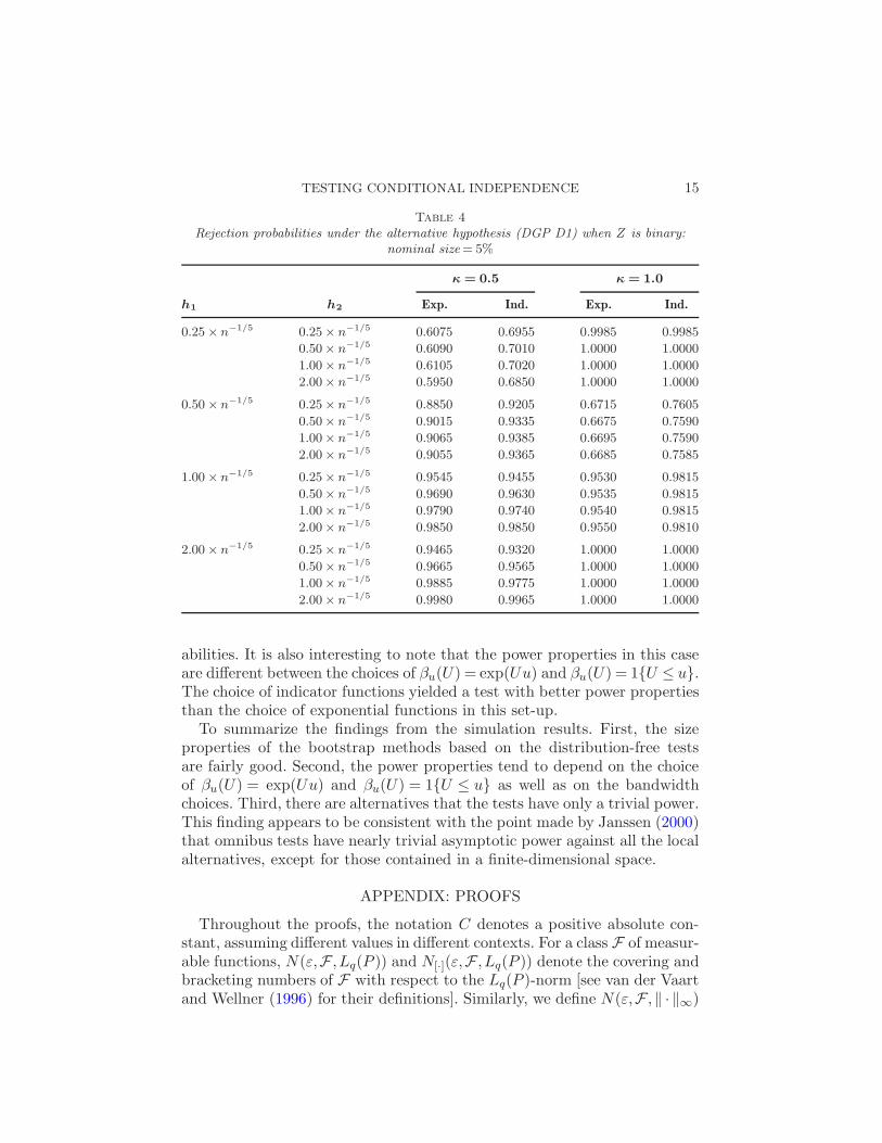
The rejection probabilities under the alternative hypothesis are presentedin Tables 4 and 5. The rejection probabilities against the alternatives DGPD1 are fairly good. It is interesting to note that the rejection probabilitiesdepend on the choice of bandwidths. The performance is almost the samefor the choice of βu(U) = exp(Uu) or βu(U) = 1{U ≤ u}.
The numbers in Table 4 show an interesting result that the bandwidthchoice for pz,i(Ui) is more important for the power property of the test
than the bandwidth for Yi. When there is more smoothing in the estima-tion of pz,i(Ui) within the range of bandwidths considered, the rejectionprobability improves. However, the rejection probabilities are not as sensi-tive to the bandwidth choices for Yi. Similar observations are made for thecase with DGP D2, where Yi relies nonlinearly on the deviation componentκs(Zi,X1i,X2i). In this case, the rejection probabilities are mostly better
when pz,i(Ui) involves more smoothing given the range of the bandwidths.However, the nonlinearity has an overall effect of reducing the rejection prob-
TESTING CONDITIONAL INDEPENDENCE 15
Table 4
Rejection probabilities under the alternative hypothesis (DGP D1) when Z is binary:nominal size = 5%
κ = 0.5 κ = 1.0
h1 h2 Exp. Ind. Exp. Ind.
0.25× n−1/5 0.25× n
−1/5 0.6075 0.6955 0.9985 0.9985
0.50× n−1/5 0.6090 0.7010 1.0000 1.0000
1.00× n−1/5 0.6105 0.7020 1.0000 1.0000
2.00× n−1/5 0.5950 0.6850 1.0000 1.0000
0.50× n−1/5 0.25× n
−1/5 0.8850 0.9205 0.6715 0.7605
0.50× n−1/5 0.9015 0.9335 0.6675 0.7590
1.00× n−1/5 0.9065 0.9385 0.6695 0.7590
2.00× n−1/5 0.9055 0.9365 0.6685 0.7585
1.00× n−1/5 0.25× n
−1/5 0.9545 0.9455 0.9530 0.9815
0.50× n−1/5 0.9690 0.9630 0.9535 0.9815
1.00× n−1/5 0.9790 0.9740 0.9540 0.9815
2.00× n−1/5 0.9850 0.9850 0.9550 0.9810
2.00× n−1/5 0.25× n
−1/5 0.9465 0.9320 1.0000 1.0000
0.50× n−1/5 0.9665 0.9565 1.0000 1.0000
1.00× n−1/5 0.9885 0.9775 1.0000 1.0000
2.00× n−1/5 0.9980 0.9965 1.0000 1.0000
abilities. It is also interesting to note that the power properties in this caseare different between the choices of βu(U) = exp(Uu) and βu(U) = 1{U ≤ u}.The choice of indicator functions yielded a test with better power propertiesthan the choice of exponential functions in this set-up.
To summarize the findings from the simulation results. First, the sizeproperties of the bootstrap methods based on the distribution-free testsare fairly good. Second, the power properties tend to depend on the choiceof βu(U) = exp(Uu) and βu(U) = 1{U ≤ u} as well as on the bandwidthchoices. Third, there are alternatives that the tests have only a trivial power.This finding appears to be consistent with the point made by Janssen (2000)that omnibus tests have nearly trivial asymptotic power against all the localalternatives, except for those contained in a finite-dimensional space.
APPENDIX: PROOFS
Throughout the proofs, the notation C denotes a positive absolute con-stant, assuming different values in different contexts. For a class F of measur-able functions, N(ε,F ,Lq(P )) and N[·](ε,F ,Lq(P )) denote the covering andbracketing numbers of F with respect to the Lq(P )-norm [see van der Vaartand Wellner (1996) for their definitions]. Similarly, we define N(ε,F ,‖ · ‖∞)

16 K. SONG
Table 5
Rejection probabilities under the alternative hypothesis (DGP D2) when Z is binary:nominal size = 5%
κ = 0.5 κ = 1.0
h1 h2 Exp. Ind. Exp. Ind.
0.25× n−1/5 0.25× n
−1/5 0.2200 0.2865 0.3040 0.4175
0.50× n−1/5 0.2225 0.2895 0.3020 0.4220
1.00× n−1/5 0.2120 0.2870 0.3020 0.4260
2.00× n−1/5 0.2150 0.2795 0.2980 0.4160
0.50× n−1/5 0.25× n
−1/5 0.3245 0.3745 0.4350 0.5560
0.50× n−1/5 0.3500 0.4075 0.4675 0.5785
1.00× n−1/5 0.3405 0.4100 0.4650 0.5975
2.00× n−1/5 0.3460 0.4125 0.4615 0.5915
1.00× n−1/5 0.25× n
−1/5 0.3490 0.3755 0.4680 0.5685
0.50× n−1/5 0.3675 0.4135 0.5020 0.6000
1.00× n−1/5 0.3820 0.4420 0.5205 0.6320
2.00× n−1/5 0.3925 0.4610 0.5275 0.6525
2.00× n−1/5 0.25× n
−1/5 0.3275 0.3600 0.4750 0.5535
0.50× n−1/5 0.3575 0.3960 0.5065 0.5815
1.00× n−1/5 0.3840 0.4445 0.5340 0.6360
2.00× n−1/5 0.4425 0.5110 0.6040 0.6995
and N[·](ε,F ,‖ ·‖∞) to be the covering and bracketing numbers with respectto ‖ · ‖∞.
A.1. Preliminary results.
Lemma A1. Let Λ be a class of measurable functions such that for eachλ ∈ Λ, λ(X) is continuous with a density function (under P ) bounded byM > 0. Let T be a class of functions of bounded variation that take valuesin [−M,M ]. Then for the class G ≡ {τ ◦λ : (τ,λ) ∈ T ×Λ}, it is satisfied thatfor any q ≥ 1,
logN[·](C2ε,G,Lq(P )) ≤ logN(εq,Λ,‖ · ‖∞) + C1/ε,
where C1 and C2 are positive constants depending only on q and M .
Proof. Let Fλ be the c.d.f. of λ(X). For any λ1, λ2 ∈ Λ,
supx
|Fλ1(λ1(x))−Fλ2(λ2(x))| ≤M‖λ1 − λ2‖∞,
because the density of λ(X), λ ∈ Λ, is uniformly bounded. From now on,we identify λ(x) with Fλ(λ(x)) without loss of generality so that λ(X) is

TESTING CONDITIONAL INDEPENDENCE 17
uniformly distributed on [0,1]. Since T ⊂ T+ − T− where T+ and T− arecollections of uniformly bounded, monotone functions, and we can write T+
and T− as unions of increasing functions and decreasing functions, we loseno generality by assuming that each τ ∈ T is decreasing. Hence by the resultof Birman and Solomjak (1967), for any q ≥ 1
logN[·](ε,T ,Lq(P )) ≤ C2
ε(13)
for a constant C2 > 0 that does not depend on P .Choose {λ1, . . . , λN1} such that any λ ∈ Λ is assigned with λj satisfying
‖λj − λ‖∞ < εq/2, and take an integer Mε ∈ [2ε−q + 1,2ε−q + 2) and a set{c1, . . . , cMε} such that c1 = 0 and
cm+1 = cm + εq/2, m = 1, . . . ,Mε − 1,
so that 0 = c1 ≤ c2 ≤ · · · ≤ cMε−1 ≤ 1 ≤ cMε . Define
λj(x) = cm when λj(x) ∈ [cm, cm+1), for some m ∈ {1,2, . . . ,Mε − 1}.
For each j1 ∈ {1, . . . ,N1}, let Pj1 be the distribution of λj1(X) under P .
Then choose {(τk,∆k)}N2(j1)k=1 such that any τ ∈ T is assigned with a bracket
(τj2 ,∆j2) satisfying |τ(λ)− τj2(λ)| ≤ ∆j2(λ) and∫
∆j2(λ)qPj1(dλ) < εq .Now, take any g ≡ τ ◦λ ∈ G and let λj1 and τj2 be such that ‖λj1 −λ‖∞ <
εq/2 and |τ − τj2| ≤ ∆j2 with∫
∆j2(λ)qPj1(dλ) < εq. Fix these j1 and j2 andextend the domain of ∆j2 to R by setting ∆j2(λ) = 0 for all λ ∈R \ [0,1].
Note that
|g(x) − (τj2 ◦ λj1)(x)|≤ |(τ ◦ λ)(x)− (τ ◦ λj1)(x)|+ |(τ ◦ λj1)(x)− (τj2 ◦ λj1)(x)|(14)
≤ |(τ ◦ λ)(x)− (τ ◦ λj1)(x)|+ (∆j2 ◦ λj1)(x).
The range of λj1 is finite and ‖λ− λj1‖∞ ≤ ‖λ− λj1‖∞ + ‖λj1 − λj1‖∞ ≤ εq.
Since τ is decreasing, |(τ ◦ λ)(x) − (τ ◦ λj1)(x)| is bounded by τ(λj1(x) −εq)− τ(λj1(x) + εq), or by
τj2(λj1(x)− εq)− τj2(λj1(x) + εq) + ∆j2(λj1(x)− εq) + ∆j2(λj1(x) + εq).
Write the difference τj2(λj1(x) − εq) − τj2(λj1(x) + εq) as A1(x) + A2(x) +A3(x) + A4(x), where
A1(x) ≡ τj2(λj1(x)− εq)− τj2(λj1(x)− εq/2),
A2(x) ≡ τj2(λj1(x)− εq/2)− τj2(λj1(x)),
A3(x) ≡ τj2(λj1(x))− τj2(λj1(x) + εq/2)

18 K. SONG
and
A4(x)≡ τj2(λj1(x) + εq/2)− τj2(λj1(x) + εq).
Due to the construction of λj1(x), we write A1(x) as
Mε−1∑
m=1
{τUm(j2)− τL
m(j2)} × 1{cm ≤ λj1(x) < cm+1},
where τUm(j2) = τj2(cm − εq) and τL
m(j2) = τj2(cm − εq/2). Since τj2 is de-creasing, τL
m(j2)≤ τUm(j2), and since cm+1 = cm + εq/2,
τUm+1(j2) = τj2(cm+1 − εq) = τj2(cm − εq/2) = τL
m(j2), m = 1, . . . ,Mε − 1.
Hence, we conclude
τLMε−1(j2) ≤ · · · ≤ τU
m+1(j2) = τLm(j2)≤ τU
m(j2) = τLm−1(j2)≤ · · · ≤ τU
1 (j2).
Suppose that τU1 (j2) = τL
Mε−1(j2). Then A1(x) = 0 and the Lq(P )-norm of
A1 is trivially zero. Suppose that τU1 (j2) > τL
Mε−1(j2). Since τj2 is uniformly
bounded, we have τU1 (j2)− τL
Mε−1(j2) < C < ∞ for some C > 0. Define
∆j1,j2(x) ≡Mε−1∑
m=1
τUm(j2)− τL
m(j2)
τU1 (j2)− τL
Mε−1(j2)× 1{cm ≤ λj1(x) < cm+1}.
Let pm(j1) ≡ P{cm ≤ λj1(X) < cm+1}. Since ∆j1,j2(x) ≤ 1, ∆qj1,j2
(x) ≤∆j1,j2(x) so that
E∆qj1,j2
(X) ≤Mε−1∑
m=1
τUm(j2)− τL
m(j2)
τU1 (j2)− τL
Mε−1(j2)× pm(j1)≤ εq/2,
because pm(j1) ≤ εq/2 for m∈ {1, . . . ,Mε − 1}. Thus the Lq(P )-norm of A1
is bounded by Cε. We can deal with the functions Aj(x), j = 2,3,4, similarlyby redefining τU
m(j2) and τLm(j2).
From (14) we can bound |g(x) − (τj2 ◦ λj1)(x)| by
A1(x) + A2(x) + A3(x) + A4(x)
+ (∆j2 ◦ λj1)(x) + ∆j2(λj1(x)− εq) + ∆j2(λj1(x) + εq)(15)
≡ ∆∗j1,j2(x).
Now, let us compute [E{∆∗j1,j2(X)}q ]1/q. The Lq(P )-norm of the first four
functions is bounded by Cε, as we proved before. By the choice of ∆j2 ,
E[∆qj2
(λj1(X))] =
∫
∆j2(λ)qPj1(dλ) < εq.

TESTING CONDITIONAL INDEPENDENCE 19
Let us turn to the last two terms in (15). Note that
E[∆qj2
(λj1(X)− εq)] =Mε−1∑
m=1
∆qj2
(cm − εq)pm(j1)
≤Mε−1∑
m=1
∆qj2
(cm − εq)εq/2 =Mε−3∑
m=1
∆qj2
(cm)εq/2
≤ E[∆qj2
(λj1(X))] < εq.
The second equality is due to our setting ∆j2(c) = 0 for c ∈ R \ [0,1]. Thesecond to the last inequality is due to the fact that pm(j1) = εq/2 for allm ∈ {1, . . . ,Mε − 2}. Similarly, E[∆q
j2(λj1(X) + εq)] < εq. Combining these
results, E[{∆∗j1,j2(X)}q ]≤Cq
1εq, for some constant C1 > 0, yielding the resultthat
logN[·](C1ε,G,Lq(P )) ≤ logN(εq/2,Λ,‖ · ‖∞) + C2/ε.
With redefinitions of constants and ε, this completes the proof. �
Given x(n) ≡ (xj)nj=1 ∈R
ndX , let
Gn,λ(·;x(n))≡1
n
n∑
j=1
1{λ(xj)≤ ·}.(16)
Lemma A1 yields the following bracketing entropy bound by taking τ =βu ◦Gn,λ. Certainly, this τ is bounded variation, because Gn,λ is increasing.
Corollary A1. Let Λ and M be as in Lemma A1, and for βu in As-sumption 2(i) let
Bn ≡ {βu(Gn,λ(λ(·);x(n))) : (u,λ,x(n)) ∈ [0,1]×Λ×RndX}.
Then logN[·](C2ε,Bn,Lq(P )) ≤ logN(εq,Λ,‖ · ‖∞) + C1/ε, for any q ≥ 1,where C1 and C2 are positive constants depending only on q and M .
The following lemma is useful for establishing a bracketing entropy boundof a class in which conditional c.d.f. estimators realize.
Lemma A2. We introduce three classes of functions. First, let Fn bea sequence of classes of maps φ(·, ·) :R × Sn → [0,1], such that (a) Sn ⊂[−sn, sn], sn > 1, (b) for each v ∈ Sn, φ(·, v) is bounded variation and (c)for each ε > 0,
sup(y,v)∈R×Sn
supη∈[0,ε]
|φ(y, v + η)− φ(y, v − η)| < Mnε(17)

20 K. SONG
for some sequence Mn > 1. Second, let G be a class of measurable functionsG :RdX →Sn. Finally, let J G
n ≡ {φ(·,G(·)) : (φ,G) ∈Fn ×G}.Then for any probability P , and for any q > 1,
logN[·](ε,J Gn ,Lq(P ))
≤ C + C log(2snMn + ε)
+ C{(2snMn + ε)1/qε−(q+1)/q − log(ε) + logN[·](Cε/Mn,G,Lq(P ))}for some C > 0.
Proof. Fix ε > 0 and take a partition Sn =⋃Jε
k=1 B(bk) where B(bk) is aset contained in an ε/Mn-interval centered at bk, and Jε ≤ 2snMn/ε+1. Let
Fn(bk)≡ {φ(·, bk) :φ ∈ Fn}. For each bk, take {(fk,j,∆k,j)}Nε(bk)j=1 such that to
any f ∈ Fn(bk) corresponds (fk,j,∆k,j) such that |f(y)− fk,j(y)| ≤ ∆k,j(y)and
∫
∆qk,j(y)P (dy) ≤ εq+1/(2snMn + ε).
Given φ ∈ Fn, we let fj(y, v) ≡∑Jεk=1 fk,j(y)Ak(v), where Ak(v) ≡ 1{v ∈
B(bk)} and fk,j(y) is such that |φ(y, bk)− fk,j(y)| ≤ ∆k,j(y) and∫
∆qk,j(y)P (dy) ≤ εq+1/(2snMn + ε).
Since Fn(bk) is a uniformly-bounded class of bounded variation functions,the smallest number of such (k, j)’s are bounded by
Jε exp
(
C(2snMn + ε)1/q
ε(q+1)/q
)
≤(
2snMn
ε+ 1
)
exp
(
C(2snMn + ε)1/q
ε(q+1)/q
)
.(18)
Then we bound |φ(y, v)− fj(y, v)| by∣
∣
∣
∣
∣
Jε∑
k=1
{φ(y, v) − φ(y, bk)}Ak(v)
∣
∣
∣
∣
∣
+
∣
∣
∣
∣
∣
Jε∑
k=1
{φ(y, bk)− fk,j(y)}Ak(v)
∣
∣
∣
∣
∣
.(19)
The second term is bounded by∑Jε
k=1 ∆k,j(y)Ak(v), and the first term, byε, due to (17). Hence
|φ(y, v)− fj(y, v)| ≤ ∆j(y, v),
where ∆j(y, v) ≡∑Jεk=1 ∆k,j(y)Ak(v) + ε. By the Holder inequality,(
Jε∑
k=1
∆k,j(y)Ak(v)
)q
≤Jε∑
k=1
∆qk,j(y).
Hence,∫
∆qj(y, v)P (dy, dv) is bounded by
CJε∑
k=1
∫
∆qk,j(y)P (dy) + Cεq ≤ CJεε
q+1
2snMn + ε+ Cεq ≤ 2Cεq,

TESTING CONDITIONAL INDEPENDENCE 21
yielding the inequality [from (18)]
logN[·](Cε,Fn,Lq(P ))(20)
≤C + log(2snMn + ε) + C(2snMn + ε)1/q/ε(q+1)/q − log(ε).
Now, take (Gk,∆k)N1k=1 such that to any G ∈ G corresponds (Gj ,∆j) such
that |G − Gj | ≤ ∆j and E∆qj(X) < (ε/Mn)q. Take (φk, ∆k)
N2(j)k=1 such that
for any φ ∈Fn, there exists (φk, ∆k) such that |φ(y, v)−φk(y, v)| < ∆k(y, v)
and E∆qk(Y,Gj(X)) < εq. Now, we bound |φ(y,G(x)) − φk(y,Gj(x))| by
|φ(y,G(x)) − φ(y,Gj(x))|+ |φ(y,Gj(x))− φk(y,Gj(x))|≤ Mn∆j(x) + ∆k(y,Gj(x)) ≡ ∆j,k(y,x).
Since E∆qj,k(Y,X)≤ Cεq, we conclude that
logN[·](Cε,J Gn ,Lq(P ))
≤C logN[·](ε,Fn,Lq(P )) + C logN[·](ε/Mn,G,Lq(P )).
Combined with (20), this yields the desired result. �
Fix λ0 :RdX →R in a uniformly bounded class Λ, and let F0 be the distri-bution function of λ0(X). Let Fn,0,i and Fn,λ,i be the empirical distributionfunctions of {λ0(Xj)}n
j=1,j 6=i and {λ(Xj)}nj=1,j 6=i, {Xj}n
j=1 being i.i.d. ∼ P .
Lemma A3. Define Λn ≡ {λ ∈ Λ:‖λ − λ0‖∞ ≤ Cn−1/2} for C > 0 andassume that Λn satisfy the conditions for Λ in Lemma A1 and that logN(Cε,Λn,‖ · ‖∞) < Cε−rΛ for some C > 0 and rΛ ∈ [0,1). Then,
E
[
max1≤i≤n
supλ∈Λn
supx∈R
dX
|Fn,λ,i(λ(x)) −F0(λ0(x))|]
= O(n−1/2).
Proof. Let every λ in Λ be bounded in [−M,M ]. It suffices to showthat
supλ∈Λn
supx∈R
dX
|Fλ(λ(x))− F0(λ0(x))| = O(n−1/2) and
(21)E
[
max1≤i≤n
supλ∈Λn
supλ∈[−M,M ]
|Fn,λ,i(λ)− Fλ(λ)|]
= O(n−1/2).
The first statement of (21) follows, due to λ0(X) having a bounded densityand supλ∈Λn
‖λ− λ0‖∞ = O(n−1/2) by the definition of Λn.As for the second statement, write
|Fn,λ,i(λ)−Fλ(λ)| ≤∣
∣
∣
∣
∣
1
n− 1
n∑
j=1,j 6=i
(1{λ(Xj)≤ λ} −P{λ(Xj)≤ λ})∣
∣
∣
∣
∣
.

22 K. SONG
For any λ1, λ2 ∈Λn and λ1, λ2 ∈ [−M,M ],
E|1{λ1(Xj)≤ λ1} − 1{λ2(Xj) ≤ λ2}| ≤ C{‖λ1 − λ2‖∞ + |λ1 − λ2|}.This implies that
logN[·](ε,Fn,L2(P )) ≤ logN(Cε2,Λn × [−M,M ],‖ · ‖∞ + | · |) ≤Cε−2rΛ ,
where Fn ≡ {1{λ(·) ≤ λ} : (λ, λ) ∈ Λ × [−M,M ]}. Since rΛ < 1, the secondresult of (21) follows from the maximal inequality of Pollard (1989) [seeTheorem A.2 of van der Vaart (1996)]. �
Let Λn, λ0, F0, and Fn,λ,i be as in Lemma A3 and define
Un,λ,i ≡ Fn,λ,i(λ(Xi)) and U ≡ F0(λ0(X))
for λ ∈ Λn. Let SW be a subset of RdW and introduce Φn, a class of functions
ϕ :SW →R. Then we define a kernel estimator of gϕ(u)≡E[ϕ(W )|U = u]:
gϕ,λ,i(u) ≡∑n
j=1,j 6=i ϕ(Wj)Kh(Un,λ,j − u)∑n
j=1,j 6=i Kh(Un,λ,j − u).(22)
The following lemma proves uniform convergence of gϕ,λ,i(u) over (ϕ,λ) ∈Φn × Λn. A related result without the transform Fn,λ,i was obtained byAndrews (1995).
Lemma A4. Let Λn be as in Lemma A3. Furthermore, assume the fol-lowing:
(A1) logN(Cε,Λn,‖ · ‖∞) < Cε−rΛ for some C > 0 and rΛ ∈ [0,1).(A2) Φn has an envelope ϕ such that ‖ϕ‖P,2 < ∞,
supu∈[0,1]
E[|ϕ(Wi)||Ui = u] < ∞,
and for some rΦ ∈ [0,2), logN[·](ε,Φn,L2(P )) < ε−rΦ .(A3) gϕ(·), ϕ ∈ Φn, is twice continuously differentiable with uniformly
bounded derivatives.(A4) K is symmetric, nonnegative, continuously differentiable, has a com-
pact support, and∫∞−∞ K(s) = 1.
Then as h→ 0 and n−1/2h−1 → 0 with n →∞,
max1≤i≤n
sup(ϕ,λ)∈Φn×Λn
|gϕ,λ,i(u)− gϕ(u)|
≤∆n(u) + O(n−1/2h−1√
− logh),
where ∆n(u) = C(h21{|u− 1|> h}+ h1{|u − 1| ≤ h}) for some C > 0.Furthermore, if Φn is uniformly bounded,
max1≤i≤n
sup(ϕ,λ)∈Φn×Λn
supu∈[0,1]
|gϕ,λ,i(u)− gϕ(u)|
≤ ∆n(u) + O(n−1/2h−1).

TESTING CONDITIONAL INDEPENDENCE 23
Proof. We consider the first statement. Without loss of generality, as-sume that K has a support in [−1,1], and K(·) ≤ M for some M > 0. ByLemma A3, it suffices to focus on the event supx |Fn,λ,i(λ(x))−F0(λ0(x))| <Mn−1/2 for large M > 0. Define
ρϕ,λ,i(u) ≡ 1
n− 1
n∑
j=1,j 6=i
Kh(Un,λ,j − u)ϕ(Wj)
and
fλ,i(u)≡ 1
n− 1
n∑
j=1,j 6=i
Kh(Un,λ,j − u).
First, let us prove that uniformly over 1 ≤ i ≤ n,
sup(ϕ,λ)∈Φn×Λn
|ρϕ,λ,i(u)− ξ1n(u)gϕ(u)|(23)
≤∆n(u) + O(n−1/2h−1√
− logh),
where ξ1n(u) =∫ ((1−u)/h)∧1(−u/h)∨(−1) K(v)dv. Write ρϕ,λ,i(u)− ξ1n(u)gϕ(u) as
1
n− 1
n∑
j=1,j 6=i
{Kh(Un,λ,j − u)−Kh(Uj − u)}ϕ(Wj)
+1
n− 1
n∑
j=1,j 6=i
Kh(Uj − u)ϕ(Wj)− ξ1n(u)gϕ(u)
≡ A1n + A2n.
We deal with A1n following the proof of Lemma 4.5 of Stute and Zhu (2005).Since K has support in [−1,1], A1n is the sum of those j’s such that either|Un,λ,j − u| ≤ h or |Uj − u| ≤ h. By Lemma A3,
max1≤j≤n,
supλ∈Λn
|Un,λ,j −Uj|= OP (n−1/2).
Since n−1/2h−1 → 0, A1n is equal to
1
(n− 1)h2
n∑
j=1,j 6=i
K ′(∆ij)ϕ(Wj){Un,λ,j −Uj}1{|Uj − u| ≤ Ch}(24)
with probability approaching one, where ∆ij lies between (Un,λ,j −u)/h and(Uj − u)/h. Therefore, by (A4), the term in (24) is bounded by
OP (n−1/2)× 1
(n− 1)h2
n∑
j=1,j 6=i
|ϕ(Wj)|1{|Uj − u| ≤ Ch}

24 K. SONG
with probability approaching one. By (A2), the expectation of the abovesum is O(h−1), yielding
A1n = OP (n−1/2h−1).(25)
This leaves us to deal with A2n which we write as
A2n =1
n− 1
n∑
j=1,j 6=i
Kh(Uj − u){ϕ(Wj)− gϕ(Uj)}
+1
n− 1
n∑
j=1,j 6=i
Kh(Uj − u)gϕ(Uj)− ξ1n(u)gϕ(u)
≡ (I) + (II).
The sum (I) is a mean-zero process. Define φu(y, v) ≡ K((y−u)/h)v, ϕ(w,u;ϕ) ≡ ϕ(w)− gϕ(u), and
Φn ≡ {ϕ(·, ·;ϕ) :ϕ ∈Φn}and
J1n ≡ {φu(·, ϕ(·)) : (u, ϕ) ∈ [0,1]× Φn}.Take J(w,u) = M{ϕ(w)+gϕ(u)} as an envelop for J1n. Then, E|J(W,U)|2 <∞. Note that
|φu1(y, ϕ(w,u;ϕ))− φu2(y, ϕ(w,u;ϕ))| ≤ C|u1 − u2||ϕ(w) + gϕ(u)|/hand
|φu(y, ϕ(w,u;ϕ1))− φu(y, ϕ(w,u;ϕ2))|≤ C|ϕ1(w)− ϕ2(w)|+ C|gϕ1(u)− gϕ2(u)|.
Since E|gϕ1(U)− gϕ2(U)|q ≤E|ϕ1(W )−ϕ2(W )|q, q ≥ 1, we conclude that
logN[·](ε,J1n,L2(P ))
≤ logN(Cεh, [0,1], | · |) + logN(Cε,Φn,L2(P ))(26)
≤ C − (log ε + logh) + Cε−rΦ .
Therefore, by the maximal inequality of Pollard (1989) [e.g., Theorem A.2of van der Vaart (1996)],
E
[
sup(u,ϕ)∈[0,1]×Φn
∣
∣
∣
∣
∣
1
n− 1
n∑
j=1,j 6=i
K
(
Uj − u
h
)
{ϕ(Wj)− gϕ(Uj)}∣
∣
∣
∣
∣
]
≤ C√n− 1
∫ C
0
√
1 + logN[·](ε,J1n,L2(P ))dε(27)
= O(n−1/2√
− logh).

TESTING CONDITIONAL INDEPENDENCE 25
Hence the uniform convergence rate for (I) is O(n−1/2h−1√− logh).
Let us turn to (II). For this, write (II) as
1
n− 1
n∑
j=1,j 6=i
{Kh(Uj − u)gϕ(Uj)−E[Kh(Uj − u)gϕ(Uj)]}
(28)+ E[Kh(Uj − u)gϕ(Uj)]− ξ1n(u)gϕ(u).
From the steps to prove (27), the first sum is OP (n−1/2h−1√− logh) uni-
formly over u ∈ [0,1]. Write the last difference in (28), for u ∈ [0,1], as
1
h
∫ 1
0K
(
v − u
h
)
gϕ(v)dv − gϕ(u)ξ1n(u) = g′ϕ(u)ξ2n(u)h + O(h2),
where ξ2n(u) =∫ ((1−u)/h)∧1(−u/h)∨(−1) vK(v)dv. Therefore,
(II) ≤∆n(u) + O(n−1/2h−1√
− logh).
Combining (I) and (II), we obtain (23).Following the proof of (23) with ϕ = 1, we also obtain
sup(ϕ,λ,u)∈Φn×Λn×[0,1]
|fλ,i(u)− ξ1n(u)| = O(n−1/2h−1√
− logh).(29)
The quantity |ξ1n(u)− 1{u ∈ [0,1]}| is bounded by
max
{∫ 1
0K(v)dv,
∫ 0
−1K(v)dv
}
≤ 1/2.
Thus ξ1n(u) ≥ 1/2 for u ∈ [0,1]. Write gϕ,λ,i(u)− gϕ(u) as
ρϕ,λ,i(u)
{
1
fλ,i(u)− 1
ξ1n(u)
}
+1
ξ1n(u){ρϕ,λ,i(u)− ξ1n(u)gϕ(u)}.
We apply (23) and (29) to the first and second terms to obtain the firstresult of the theorem.
As for the second result, we modify the treatment of (I) above. Note that
sup(y,v)∈R×[−sn,sn]
supη∈[0,ε]
|φu(y, v + η)− φu(y, v − η)| ≤ Cε.
Since K(·) is Lipschitz, it is bounded variation, and so are K((· − u)/h).Since Φn is uniformly bounded, we apply Lemma A2 (with sn equal to somelarge M > 0),
logN[·](ε,J1n,L2(P )) ≤ C + C{ε−3/2 − log(ε) + ε−rΦ}.Substituting this bound for the one in (26) and following the same argumentsthere, we obtain the wanted result. �

26 K. SONG
Let Λ be a uniformly bounded class of real functions and fix λ0 ∈ Λ.Let SX be the support of a random vector X , and [0,1]2 be the supportof a random vector (Z, Y ). Let fλ(z|y, λ1, λ0) be the conditional densityof Z given Y = y,λ1(X) = λ1 and λ0(X) = λ0 with respect to a σ-finiteconditional measure. Introduce
µλ(z|y, λ1, λ0)≡E[γz(Z)|Y = y,λ(X) = λ1, λ0(X) = λ0]
and
µλ(z|y, λ0) ≡E[γz(Z)|Y = y,λ0(X) = λ0].
For each λ ∈Λ,S(λ) be the support of λ(X).
Lemma A5. Suppose that there exists C > 0 such that for each λ1 ∈ Λ,each δ > 0 and each (λ1, λ0) ∈ S(λ1)×S(λ0),
sup(z,y,λ1)∈[0,1]2×S(λ1) : |λ1−λ1|<δ
|fλ1(z|y, λ1, λ0)− fλ1(z|y, λ1, λ0)| ≤ Cδ.
Then for each δ > 0 and each λ1 in Λ such that ‖λ1 − λ0‖∞ ≤ δ,
sup(z,y,x)∈[0,1]2×SX
|µλ1(z|y,λ1(x), λ0(x))− µλ0(z|y,λ0(x))| ≤ 6Cδ.
Proof. Choose (z, y, x) ∈ [0,1]2 × SX and λ1 ∈ Λ with ‖λ1 − λ0‖∞ < δand let λ0 ≡ λ0(x) and λ1 ≡ λ1(x). Let Py be the conditional measure of
(Z,X) given (Y , λ0(X)) = (y, λ0) and Ey be the conditional expectationunder Py . Let Aj ≡ 1{|λj(X)− λj | ≤ 3δ}, j = 0,1. Note that Ey[A0] = 1 and
1 ≥Ey[A1] = P{|λ1(X)− λ1| ≤ 3δ|Y = y,λ0(X) = λ0}≥ P{|λ0(X)− λ0| ≤ δ|Y = y,λ0(X) = λ0} = 1.
Let µλj(z|y, λj , λ0)≡Ey[γz(Z)Aj ]/Ey[Aj ] = Ey[γz(Z)Aj ], j = 0,1. Then, for
example,
|µλ1(z|y, λ1, λ0)− µλ0(z|y, λ0)|≤ |µλ1(z|y, λ1, λ0)− µλ1(z|y, λ1, λ0)|+ |µλ1(z|y, λ1, λ0)− µλ0(z|y, λ0)|≡ (I) + (II).
Let us turn to (I). By the definition of conditional expectation,
µλ1(z|y, λ1, λ0) =
∫ λ1+3δ
λ1−3δµλ1(z|y, λ, λ0)dFλ1(λ|y, λ0),
where Fλ1(·|y, λ0) is the conditional c.d.f. of λ1(X) given (Y , λ0(X)) =
(y, λ0). Because∫ λ1+3δλ1−3δ
dFλ1(λ|y, λ0) = Ey[A1] = 1 and |γz(Z)| ≤ 1, wp 1,
(I) ≤ supv∈[−3δ,3δ] : λ1+v∈S(λ1)
|fλ1(z|y, λ1 + v, λ0)− fλ1(z|y, λ1, λ0)|.

TESTING CONDITIONAL INDEPENDENCE 27
Therefore, by the condition of the lemma, (I)≤ 3Cδ.Let us turn to (II) which we write as
|Ey[γz(Z)A1]−Ey[γz(Z)]| = |Ey[V A1]|,
where V ≡ γz(Z)−Ey[γz(Z)] because Ey[A1] = 1. The term (II) is boundedby the absolute value of
∫ λ1+3δ
λ1−3δE[V A1|Y = y,λ1(X) = λ, λ0(X) = λ0]dFλ1(λ|y, λ0)
=
∫ λ1+3δ
λ1−3δE[V |Y = y,λ1(X) = λ, λ0(X) = λ0]dFλ1(λ|y, λ0),
or by 3Cδ, similarly as before. This implies that (II) ≤ 3Cδ. �
A.2. Proofs of the main results.
Proof of Theorem 1. (i) We first prove the following three claims:
C1. sup(θ,x)∈B(θ0,Cn−1/2)×RdX |Fn,θ,i(λθ(x))−F0(λ0(x))| = OP (n−1/2).
C2. 1√n
∑ni=1 βu(Ui){γz(Zi)− γz(Zi)}γ⊥
y (Yi) = oP (1).
C3. 1√n
∑ni=1 βu(Ui){γy(Yi)− γy(Yi)}{γz(Zi)− γz(Zi)} = oP (1).
The oP (1)’s in C2 and C3 are uniform in (u, y, z) ∈ [0,1]3.
Proof of C1. Let Λn ≡ {λθ :θ ∈ B(θ0,Cn−1/2)}. By Assumption 1(ii)(a),
logN[·](ε,Λn,‖ · ‖∞)≤ logN[·](Cε,B(θ0,Cn−1/2),‖ · ‖) ≤−C log ε,(30)
because B(θ0,Cn−1/2) is compact. Hence C1 follows by Lemma A3.
For the proofs for C2 and C3, we assume that Ui, Zi, and Yi are estimatorsusing the whole sample, not leave-one-out estimators. The discrepancy dueto this assumption is easily shown to be asymptotically negligible.
Proof of C2. Observe that
∆In,i(x; θ) ≡ sup
y∈R
|FY |U,i(y|Fn,θ,i(λθ(x)))−FY |U (y|F0(λ0(x)))|
≤ supy∈R
|FY |U,i(y|Ui)− FY |U(y|Ui)|
+ supy∈R
|FY |U (y|Ui)−FY |U (y|Ui)|
≤ supy∈R
|FY |U,i(y|Ui)− FY |U(y|Ui)|+ OP (n−1/2)

28 K. SONG
by C1 and Assumption 2(ii). Take large M > 0 and let
vn(u)≡ M(h21{|u − 1| ≥ h/2}+ h1{|u − 1| < 2h}+ n−1/2h−1).(31)
By C1 and Lemma A4, with large probability,
supθ∈B(θ0,Mn−1/2)
∆In,i(Xi, θ)≤ vn(Ui) for all i = 1, . . . , n.(32)
Take large M such that√
nhM = o(1) and expand the sum in C2 as, forexample,
M−1∑
s=1
B1n,s +zM+1
M !√
n
n∑
i=1
βu(Ui) exp(Ziz){Zi − Zi}Mγ⊥y (Yi)
≡B1n + B2n,
where Zi lies between Zi and Zi and
B1n,s ≡zs+1
s!√
n
n∑
i=1
βu(Ui) exp(Ziz){Zi − Zi}sγ⊥y (Yi).
Note that B2n = OP (√
nhM ) = oP (1) by Lemma A4. We consider B1n,s. Fixc > 0. Given x(n) ∈ R
ndX , let Gθ(·;x(n)) ≡ Gn,λ(λ(·);x(n)) with λ = λθ in(16). Denote
G1n ≡ {Gθ(·;x(n)) : (x(n), θ) ∈RndX ×B(θ0,Mn−1/2)}.
Then let Gn be the collection of G’s in G1n such that ‖G−G0‖∞ ≤Mn−1/2,where G0 = F0 ◦ λ0. Define Bn ≡ {βu ◦G : (u,G) ∈ [0,1]×Gn}. By CorollaryA1 and (30),
logN[·](ε,Bn,L2(P )) ≤ Cε−1 −C log ε.(33)
Fix a small c > 0 and let Xn ⊂ RndX × Gn be the collection of (x(n),G)’s
such that G ∈ Gn and
1
n
n∑
j=1
Kh(G(xj)− u) > c > 0.(34)
Define J G1n to be the set,
{φ(·,G(·); z(n), x(n),G) : (z(n), x(n),G) ∈Rn ×Xn},
where z(n) = {zj}nj=1 and
φ(z,u; z(n), x(n),G)≡∑n
j=1 γz(zj)Kh(G(xj)− u)∑n
j=1 Kh(G(xj)− u).

TESTING CONDITIONAL INDEPENDENCE 29
Then let J Gn ⊂J G
1n be the class of functions φ(·,G(·)) satisfying
|φ(·,G(·)) −FZ|U (·|G0(·))| ≤ vn(G0(·)).(35)
Fix any arbitrarily small w > 0. By Assumption 3(i), Lemma A4, the factthat |ξ1n(u)| ≥ 1/2 there, and (32), from sufficiently large n on,
P{FZ|U,i(·|Fn,θ(λθ(·))) ∈ J Gn } > 1−w
by increasing M in the definition of J Gn sufficiently. We will now compute a
bracketing entropy bound for J Gn .
We apply Corollary A1 and (30) to obtain that
logN[·](ε,Gn,Lq(P )) ≤−C log ε + C1/ε.(36)
Note that φ ∈ J Gn is uniformly bounded [under the restriction (34)] and
φ(z,u; z(n), x(n),G) is increasing in z for all u and that by (34),
|φ(z, v + η; z(n), x(n),G)− φ(z, v − η; z(n), x(n),G)| ≤ Cη/h3.
Take q > 3 and apply Lemma A2 and (36) to obtain that
logN[·](ε,J Gn ,L2(P ))
≤ logN[·](Cε,J Gn ,Lq(P ))(37)
≤−C log ε−C logh + Ch−3/qε−(q+1)/q.
Let ϕ0(Z,X) ≡ FZ|U (Z|G0(X)) and
fβ,z,y,ϕ(X,Z, Y ) ≡ zs+1β(X)eϕ0(Z,X)z{ϕ(Z,X) − ϕ0(Z,X)}sγ⊥y (Y ).
Let Πn ≡ {fβ,z,y,ϕ : (β, z, y,φ) ∈ Bn × [0,1]2 × J Gn }. We take its envelope to
be vsn(G0(·)), for which we observe that
E[v2sn (G0(X))] =
∫ 1
0v2sn (u)du = O(h2s+1).(38)
For Γ ≡ {γy :y ∈ [0,1]}, logN[·](ε,Γ,L2(du)) ≤ −C log ε, with du denotingthe Lebesgue measure on [0,1]. Using this, (33) and (37), we conclude that
logN[·](ε,Πn,L2(P )) ≤Ch−3/qε−(q+1)/q −C logh−C log ε.(39)
Now, let us prove that B1n,s = oP (1), s = 1, . . . ,M − 1. With large proba-bility,
B1n,s ≤ supf∈Πn
|√
n(Pn −P)f |+ supf∈Πn
|√
nPf |,

30 K. SONG
where Pn denotes the empirical measure of (Zi, Yi,Xi)ni=1. Hence by the
maximal inequality [Pollard (1989); see also Theorem A.2 of van der Vaart(1996)] and by (38) and (39),
supf∈Πn
|√
n(Pn −P)f | ≤Ch−3/(2q)∫ Chs+1/2
0ε−(q+1)/(2q) dε + o(1) = o(1).
We conclude that B1n,s ≤√
n supf∈Πn|Pf | + oP (1). By (35), the absolute
value on the right-hand side is bounded by
E[|γz,vn(Zi;Ui)||E[γ⊥y (Yi)|Zi, λθ(Xi), λ0(Xi)]|] ≤ I + II,(40)
where γz,vn(z;u)≡ zs+1ez×zvn(u)s,
I ≡E[|γz,vn(Zi;Ui)||E[γy(Yi)|Zi, λ0(Xi)]|]and
II≡E[|γz,vn(Zi;Ui)||E[γy(Yi)|Zi, λθ(Xi), λ0(Xi)]−E[γy(Yi)|Zi, λ0(Xi)]|].Term I is bounded by
o(1)×(
supz,y,u
|E[γ⊥y (Yi)|Zi = z,Ui = u]|
)
= o(1)×O(n−1/2) = o(n−1/2),
under the null hypothesis or the local alternatives of the theorem. By As-sumption 1(iii) with the aid of Lemma A5, term II is bounded by
E[|γz,vn(Zi;Ui)|]×C‖λθ − λ0‖∞ = o(n−1/2)
uniformly over (z, y, θ) ∈ [0,1]2 × B(θ0,Mn−1/2). Therefore, B1n,s = oP (1),completing the proof. �
Proof of C3. With large probability, the absolute value of the sum inC3 is bounded by
C√n
n∑
i=1
γy,vn(Yi,Ui)γz,vn(Zi,Ui) + oP (1),
where γy,vn(y;u)≡ γy(y − vn(u))− γy(y + vn(u)). Define J2n ≡ {γy,vn(·, ·)×γz,vn(·, ·) : (z, y) ∈ [0,1]2}. Note that
Pφ2 ≤CE[γy,vn(Yi,Ui)γz,vn(Zi,Ui)] = O(h3)→ 0 for each φ ∈ J2n.
This implies that the finite-dimensional distributions of {√n(Pn −P)φ :φ ∈J2n} converge in distribution to zero. By Theorem 3.3 of Ossiander (1987),√
n(Pn−P)φ is asymptotically tight in l∞(J2n) because φ ∈ J2n is uniformlybounded and
logN[·](ε,J2n,L2(P )) ≤ 2 logN[·](Cε,Γ,L2(P )) ≤−C log ε.(41)

TESTING CONDITIONAL INDEPENDENCE 31
Hence supφ∈J2n|√n(Pn −P)φ| = oP (1). We are left with
√nPφ to analyze.
Let 1n = 1{|Ui−1| ≥ 2h}. Under the null hypothesis or the local alternativesin the theorem,
√nPφ =
√nE[γy,vn(Yi,Ui)γz,vn(Zi,Ui)]
=√
nE[γy,vn(Yi,Ui)E[γz,vn(Zi,Ui)|Yi,Ui]1n]
+√
nE[γy,vn(Yi,Ui)E[γz,vn(Zi,Ui)|Yi,Ui](1− 1n)]
= O(√
nw2n) + O(
√nh3) + O(h) = o(1), wn ≡ n−1/2h−1,
because the expectation of 1{|Ui−1| < 2h} is O(h) and n−1/2h−2 +n1/2h3 →0 as n →∞ by Assumption 3(ii)(b). Hence supφ∈J2n
√nPφ = o(1), estab-
lishing C3.Now we turn to the proof of Theorem 1. Without loss of generality, let
βu be monotone decreasing. First we write νn(r)− νn(r) as
1√n
n∑
i=1
βu(Ui){γ⊥z (Zi)γ
⊥y (Yi)− γ⊥
z (Zi)γ⊥y (Yi)}
+1√n
n∑
i=1
{βu(Ui)− βu(Ui)}γ⊥z (Zi)γ
⊥y (Yi)(42)
≡A1n + A2n.
We show that Ajn = oP (1), j = 1,2. Write γ⊥z (Zi)γ
⊥y (Yi)− γ⊥
z (Zi)γ⊥y (Yi) as
{γ⊥z (Zi)− γ⊥
z (Zi)}γ⊥y (Yi)
+ {γ⊥z (Zi)− γ⊥
z (Zi)}{γ⊥y (Yi)− γ⊥
y (Yi)}(43)
+ {γ⊥y (Yi)− γ⊥
y (Yi)}γ⊥z (Zi).
By decomposing A1n into three terms according to the decomposition in(43) and applying C2 and C3, we obtain that A1n = oP (1).
As for A2n, define
J1n ≡ {((βu ◦G)− βu)γ⊥y γ⊥
z : (G,u, y, z) ∈ Gn × [0,1]3}.Following the arguments used to show supf∈Πn
|√n(Pn − P)f | = oP (1) inthe proof of C2, we can write
|A2n| ≤ supf∈J1n
√n|Pf |+ oP (1).
Similarly, as in the steps in and below (40), the leading term above is oP (1)due to the fact that
sup(z,y,u)∈[0,1]3
|E[γ⊥y (Yi)γ
⊥z (Zi)|Ui = u]|= O(n−1/2)

32 K. SONG
under the null hypothesis and the local alternatives and the fact that
sup(G,u)∈Gn×[0,1]
E[|βu(G(Xi))− βu(Ui)|]
≤ supu∈[0,1]
∫ 1
0{βu(u + Mn−1/2)− βu(u−Mn−1/2)}du = O(n−1/2),
which follows because βu is increasing and bounded in [0,1].(ii) Clearly the class J ≡ {βuγ⊥
y γ⊥z : (u, y, z) ∈ [0,1]3} is P -Donsker be-
cause its element is a product of uniformly bounded monotone functions.The weak convergence of νn(r) immediately follows, and the weak conver-gence of νn(r) follows from (i). �
Proof of Theorem 2. Let ν0∗n,b(r)≡ 1√
n
∑ni=1 ωi,bβu(Ui)γ
⊥z (Zi)γ
⊥y (Yi).
Also let Pω be the distribution of (ωi,b)ni=1 and Eω be the associated expec-
tation. It suffices to show that for each ε > 0,
Pω
{
supr∈[0,1]3
|ν∗n,b(r)− ν0∗
n,b(r)|> ε}
= oP (1).(44)
This is because the class J is P -Donsker as we saw in the proof of The-orem 1(ii), and by the conditional multiplier uniform CLT of Ledoux andTalagrand (1988) [e.g., Theorem 2.9.7 in van der Vaart and Wellner (1996)],
d(F ∗Γν0∗
n, FΓν) = o(1) a.s.
We turn to (44). Let Si = (Ui,Zi, Yi, Ui, Zi, Yi) and
ξi(r)≡ ξ(Si; r)≡ βu(Ui)γ⊥z (Zi)γ
⊥y (Yi)− βu(Ui)γ
⊥z (Zi)γ
⊥y (Yi).
Then note that for all r ∈ [0,1]3,
Eω
[∣
∣
∣
∣
∣
1√n
n∑
i=1
ωi,bξ(Si; r)
∣
∣
∣
∣
∣
2]
=1
n
n∑
i=1
ξ(Si; r)2 →P 0,(45)
using the proof of Theorem 1. Let ρn(r1, r2) =√
1n
∑ni=1(ξi(r1)− ξi(r2))2.
Observe that
−√
5− 1
2|ξi(r1)− ξi(r2)| ≤ ωi,b(ξi(r1)− ξi(r2))≤
√5 + 1
2|ξi(r1)− ξi(r2)|.
By Hoeffding’s inequality [e.g., Lemma 3.5 of van de Geer (2000), page 33],
Pω
{∣
∣
∣
∣
∣
1√n
n∑
i=1
ωi,b(ξi(r1)− ξi(r2))
∣
∣
∣
∣
∣
> ε
}
≤ exp
(
− 4ε2
(√
5 + 1)2ρn(r1, r2)2
)
.
Therefore, the process ν∗n,b(r) is sub-Gaussian with respect to ρn.

TESTING CONDITIONAL INDEPENDENCE 33
Let us compute the covering number of [0,1]3 with respect to ρn. Let Pn
be the empirical measure of (Ui,Zi, Yi, Ui, Zi, Yi)ni=1. Observe that ξ(·; r) is
bounded variation, so that for Ξ = {ξ(·; r) : r ∈ [0,1]3},
logN[·](ε,Ξ,L2(Pn))≤ C
ε.
Since ρ2n(r, rj) = ‖ξ(·; r)− ξ(·; rj)‖2
Pn,2, this implies that logN(ε, [0,1]3, ρn)≤C/ε.
Now, using Corollary 2.2.8 of van der Vaart and Wellner [(1996), page101], for any r0 ∈ [0,1]3,
Eω
[
supr∈[0,1]3
∣
∣
∣
∣
∣
1√n
n∑
i=1
ωi,bξ(Si; r)
∣
∣
∣
∣
∣
]
(46)
≤Eω
[∣
∣
∣
∣
∣
1√n
n∑
i=1
ωi,bξ(Si; r0)
∣
∣
∣
∣
∣
]
+ C
∫ ∞
0
√
logD(ε, ρn)dε,
where C is an absolute constant and D(ε, ρn) is an ε-packing number of[0,1]3 with respect to ρn. The leading term on the right-hand side vanishesin probability by (45). As for the second term, note that
supr1,r2∈[0,1]3
ρn(r1, r2)→P 0 as n→∞
from the proof of Theorem 1. Therefore, we can take δn → 0 such that
P{
supr1,r2∈[0,1]3
ρn(r1, r2) < δn
}
→ 1.
With probability approaching one,
∫ ∞
0
√
logD(ε, ρn)dε =
∫ Cδn
0
√
logD(ε, ρn)dε≤ C
∫ Cδn
0ε−1/2 dε→ 0.
We conclude that the expectation on the left-hand side of (46) vanishes inprobability. We obtain (44). �
Proof of Theorem 3. We first show that supr∈[0,1]2×Z |νn(r)− ν0n(r)|=
oP (1) both under H0 and the local alternatives in the theorem, where
ν0n(r) =
1√n
n∑
i=1
βu(Ui){1{Zi = z} − pz(Ui)}γ⊥y (Yi)
√
pz(Ui)− pz(Ui)2.
By Lemma A4, supu∈[0,1] supz∈Z |pz,i(u) − pz(u)| ≤ vn(u) where vn(u) is asdefined in (31). By Assumption 1D(iv), pz,i(u) ∈ (ε/2,1 − ε/2), ε > 0, with

34 K. SONG
probability approaching one. We introduce Gθ(·) and Gn as in the proof ofTheorem 1. Define
φz(u)≡∑n
j=1 1{zj = z}Kh(Gθ(xj)− u)∑n
j=1 Kh(Gθ(xj)− u).
Let J Gn,2 be the class of functions φz(Gθ(·)) with ({(x⊤
j , zj)⊤}n
j=1, θ) running
in (RdX ×Z)n ×B(θ0,Mn−1/2) and such that for some c > 0,
1
n
n∑
j=1
Kh(Gθ(xj)− u) > c > 0
and |φz(Gθ(·)) − pz(·)| ≤ vn(G0(·)). By Lemma A2, for any w > 0, we canfind large M such that
P{pz,i(Fn,θ,i(λθ(·))) ∈ J Gn,2}> 1−w,
logN[·](ε,J Gn,2,L2(P )) ≤ Ch−3/qε−(q+1)/q for some q > 3 and for all π(·) ∈
J Gn,2,
0 < ε/2 < infx∈R
dX
|π(x)| ≤ supx∈R
dX
|π(x)| < 1− ε/2 < 1
from some sufficiently large n on. Define
�Bn ≡ {βu,z(G(·), ·, ·;π) : (u, z, π,G) ∈ [0,1]×Z×J Gn,2 ×Gn},
where βu,z(u, z, x;π) ≡ βu(u){1{z = z}−π(x)}/√
π(x)− π2(x). Then we canwrite
νn(r) =1√n
n∑
i=1
βu,z(Ui,Zi,Xi; pz,i ◦ (Fn,θ,i ◦ λθ))γ⊥y (Yi).
To show that it is asymptotically equivalent to ν0n(r) uniformly over r ∈
[0,1]2 ×Z , we consider the following process:
1√n
n∑
i=1
β(Zi,Xi)γ⊥y (Yi), (y,β) ∈ [0,1]× �Bn.(47)
Note that βu,z(u, z, x;π) is Lipschitz in π ∈ (ε/2,1 − ε/2) with a uniformly
bounded coefficient. Therefore, logN[·](ε,�Bn,L2(P )) is bounded by
logN[·](Cε,J Gn,2,L2(P )) + logN[·](Cε,Bn,L2(P ))
(48)≤ Ch−3/qε−(q+1)/q + Cε−1 −C log ε,
where Bn was defined prior to (33). Using this bound and proceeding with
the proof of Theorem 1(i) by replacing γ⊥z by 1 and Bn by �Bn, we conclude
that νn is asymptotically equivalent to ν0n.

TESTING CONDITIONAL INDEPENDENCE 35
Let Jz ≡ {βu(·)γ⊥y (·){1{· = z} − pz(·)}/
√
pz(·)− pz(·)2 : (y,u) ∈ [0,1]2}.Then,
logN[·](ε,Jz,L2(P )) ≤ Cε−1.
Therefore,⋃
z∈Z Jz is P -Donsker because Z is a finite set. The weak con-vergence of ν0
n to ν follows. The weak convergence of νn to ν follows fromits asymptotic equivalence with ν0
n. �
Proof of Theorem 4. The proof is almost the same as the proof ofTheorem 2. We omit the details. �
Acknowledgments. I thank an Associated Editor and a referee for theircomments. I am grateful to Yoon-Jae Whang and Guido Kuersteiner whogave me valuable advice at the initial stage of this research. All errors aremine.
REFERENCES
Andrews, D. W. K. (1995). Nonparametric kernel estimator for semiparametric models.Econometric Theory 11 560–595. MR1349935
Angrist, J. D. and Kuersteiner, G. M. (2004). Semiparametric causality tests usingthe policy propensity score. NBER Working Paper 10975.
Angus, J. E. (1994). The probability integral transform and related results. SIAM Rev.36 652–654. MR1306928
Bierens, H. J. (1990). A consistent conditional moment test of functional form. Econo-metrica 58 1443–1458. MR1080813
Birman, M. S. and Solomjak, M. Z. (1967). Piecewise-polynomial approximation offunctions of the classes W
αp . Mat. Sb. (N.S.) 73 331–355. MR0217487
Blum, J. R., Kiefer, J. and Rosenblatt, M. (1961). Distribution-free tests of indepen-dence based on the sample distribution function. Ann. Statist. 32 485–498. MR0125690
Chiappori, P.-A. and Salanie, B. (2000). Testing for asymmetric information in insur-ance markets. J. Political Economy 108 56–78.
de la Pena, V. H. and Gine, E. (1999). Decoupling: From Dependence to Independence.Springer, New York. MR1666908
Delgado, M. A. and Gonzalez Manteiga, W. (2001). Significance testing in nonpara-metric regression based on the bootstrap. Ann. Statist. 29 1469–1507. MR1873339
Delgado, M. A. and Mora, J. (2000). A nonparametric test for serial independence ofregression errors. Biometrika 87 228–234. MR1766845
Gine, E. (1997). Lecture Notes on Some Aspects of the Bootstrap. Ecole de Ete de Calculde Probabilites de Saint-Flour. Lecture Notes in Mathematics 1665. Springer, Berlin.
Hardle, W. and Mammen, E. (1993). Comparing nonparametric versus parametric re-gression fits. Ann. Statist. 21 1926–1947. MR1245774
Heckman, J. J., Ichimura, H. and Todd, P. (1997). Matching as an econometric eval-uation estimator: Evidence from evaluating a job training programme. Rev. Econom.Stud. 64 605–654. MR1623713
Hoeffding, W. (1948). A nonparametric test of independence. Ann. Math. Statist. 19
546–557. MR0029139

36 K. SONG
Hong, Y. and White, H. (2005). Asymptotic distribution theory for nonparametric en-troy measures of serial dependence. Econometrica 73 837–901. MR2135144
Janssen, A. (2000). Global power functions of goodness-of-fit tests. Ann. Statist. 28 239–253. MR1762910
Khmaladze, E. V. (1993). Goodness of fit problem and scanning innovation martingales.Ann. Statist. 21 798–829. MR1232520
Lauritzen, S. L. (1996). Graphical Models. Oxford Univ. Press, New York. MR1419991Ledoux, M. and Talagrand, M. (1988). Un critere sur les pertite boules dans le
theoreme limite central. Probab. Theory Related Fields 77 29–47. MR0921817Linton, O. and Gozalo, P. (1997). Conditional independence restrictions: Testing and
estimation. Discussion Paper 1140, Cowles Foundation for Research in Economics, YaleUniv.
Ossiander, M. (1987). A central limit theorem under metric entropy with L2 bracketing.Ann. Statist. 15 897–919. MR0893905
Pearl, J. (2000). Causality: Modeling, Reasoning, and Inference. Cambridge Univ. Press,New York. MR1744773
Pollard, D. (1989). A maximal inequality for sums of independent processes under abracketing entropy condition. Unpublished manuscript.
Robinson, P. M. (1991). Consistent nonparametric entropy-based testing. Rev. Econom.Stud. 58 437–453. MR1108130
Rosenblatt, M. (1952). Remarks on a multivariate transform. Ann. Math. Statist. 23
470–472. MR0049525Skaug, H. J. and Tjøstheim, D. (1993). A nonparametric test of serial independence
based on the empirical distribution function. Biometrika 80 591–602. MR1248024Stinchcombe, M. B. and White, H. (1998). Consistent specification testing with nui-
sance parameters present only under the alternative. Econometric Theory 14 295–325.MR1628586
Stute, W., Gonzalez Manteiga, W. and Quindimil, M. P. (1998). Bootstrap approxi-mations in model checks for regression. J. Amer. Statist. Assoc. 93 141–149. MR1614600
Stute, W. and Zhu, L. (2005). Nonparametric checks for single-index models. Ann.Statist. 33 1048–1083. MR2195628
Su, L. and White, H. (2008). A nonparametric Hellinger metric test for conditionalindependence. Econometric Theory 24 829–864. MR2428851
van de Geer, S. (2000). Empirical Processes in M-Estimation. Cambridge Univ. Press,New York.
van der Vaart, A. (1996). New Donsker classes. Ann. Probab. 24 2128–2140. MR1415244van der Vaart, A. W. and Wellner, J. A. (1996). Weak Convergence and Empirical
Processes. Springer, New York. MR1385671Zhang, Z. (2008). Quotient correlation: A sample based alternative to Pearson’s correla-
tion. Ann. Statist. 36 1007–1030. MR2396823
Department of Economics
University of Pennsylvania
528 McNeil Builing
3718 Locust Walk
Philadelphia, Pennsylvania 19104
USA
E-mail: [email protected]