Mikko Laiterä 63707A Helsinki University of Technology Basics for the Biosystems of the Cell S-114.2500 Exercise

Modelling glycolysis with Cellware

2

Contents 1. Abstract 2. Glycolysis 2.1. Introduction to glycolysis 2.2. Reactions and stoichiometry of glycolysis 2.3. Regulation of glycolysis 3. Cellware 3.1. Introduction to Cellware 3.2. Reaction kinetics applied in the model 3.3. Mathematical methods for simulation 4. Modelling glyoclysis with Cellware 4.1. Constructing a model 4.2. Simulation of glycolysis 5. Discussion 6. References

3

1. Abstract Recent advances in biological sciences and information technology have made the development of “computer assisted biology” possible and the research performed this way is often referred to be done “in silico”. Computers were initially used mostly for storing information but their capability to solve numerical problems soon opened new opportunities to apply their rapidly increasing power to understand the phenomena in organisms. This development also urged the need to formulate physical and chemical laws of metabolism in the language of mathematics. The particular approach in which models are constructed to cover whole biological networks is known as systems biology. The term “glycolysis” is derived form Greek words glyk meaning sweet and lysis for dissolution. In consistent with this logic, glycolysis is the sequence of reactions that metabolizes one molecule of glucose to two molecules of pyruvate with the concomitant net production of two molecules of ATP [1]. Glycolysis is employed by a great variety of organisms, both aerobic and anaerobic, making it the most common metabolic reaction pathway in living things. In aerobic species the two pyruvate moleucles are further oxidised into carbon dioxide (CO2) in citric acid cycle and their reducing power harnessed in form of activated carriers of electrons (FADH2 and NADH) to faciliate oxidative phosphorylation. In anaerobic conditions pyruvate is converted to ethanol or to lactate (e.g. in muscle cells during anaerobic exercise). The degree of glycolysis or gluconeogenesis, synthesis of glucose from pyruvate, employed in a cell is also tightly controlled. The goal of chapter two was to review glycolysis profoundly enough to introduce basics needed to understand the model constructed and results of the simulation represented in chapter four. The Cellware program is a non-commercial graphical systems biology tool for modelling and simulation. It is rather easy to use after learning to avoid few irritating bugs. The program is also designed to serve scientists with little programming experience. Probably the user-friendliness of the program is its most important feature. To solve differential equations derived from laws of physical chemistry the Cellware simulation engine is harnessed with classical algorithms (e.g. 4th order Runge-Kutta) and a few interesting modern methods. Also for phenomena including randomness stochastic algorithms are available. The chapter three concerning Cellware is mostly about theoretical features not explained in the Cellware manual. These subjects are also applicable in other systems biology tools in general. The chapter four is about modelling glycolysis with Cellware. The objective was to show that in silico methods can faciliate better understanding of biological phenomena and even produce new information. The most difficult problem in modelling glycolysis with the Cellware was to acquire suitable equations and parameters to describe each reaction. Fortunately, the efforts were rewarded and the results of the simulation gave insight to the qualitative variation of concentrations of metabolites during reaction. Probably more importantly the simulation supported the common practice of dividing glycolysis into two different phases. Also at least one reference to the allosteric control in the model of glycolysis was discovered.

4

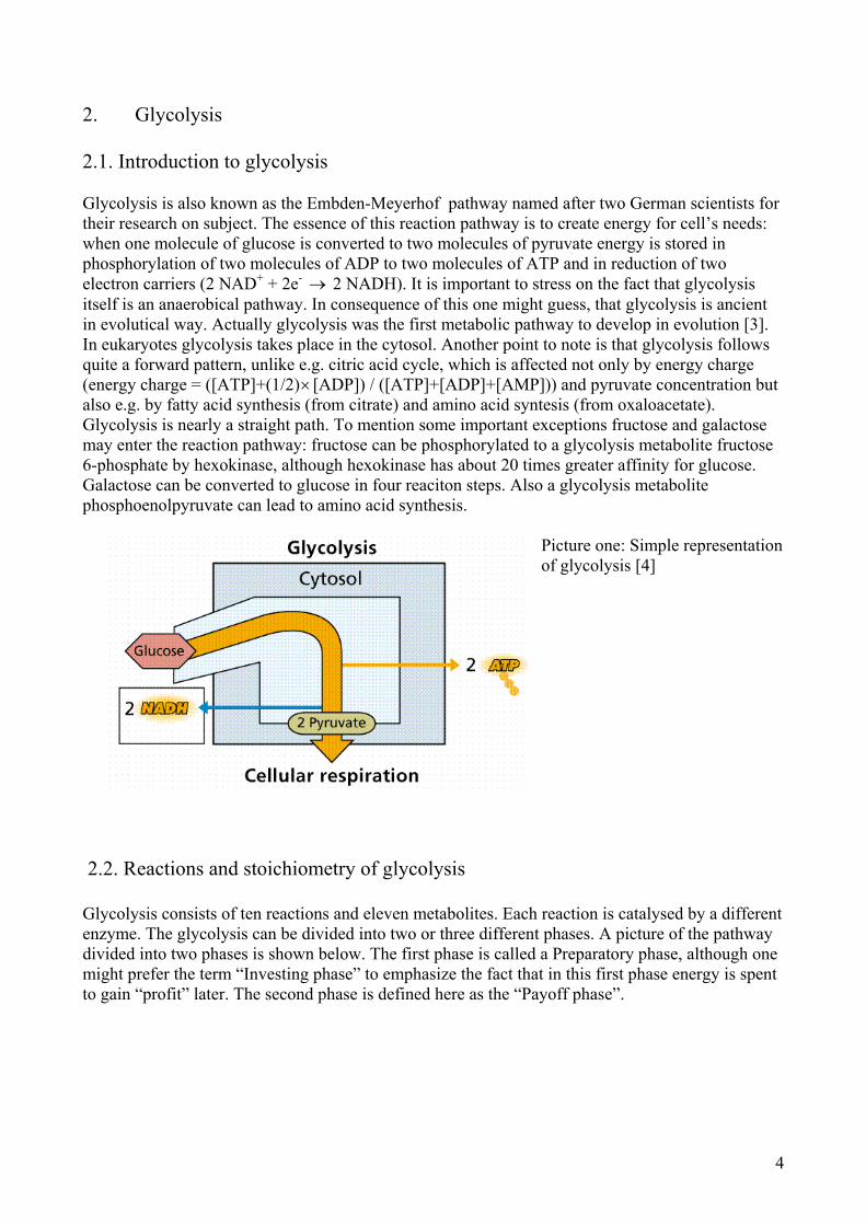
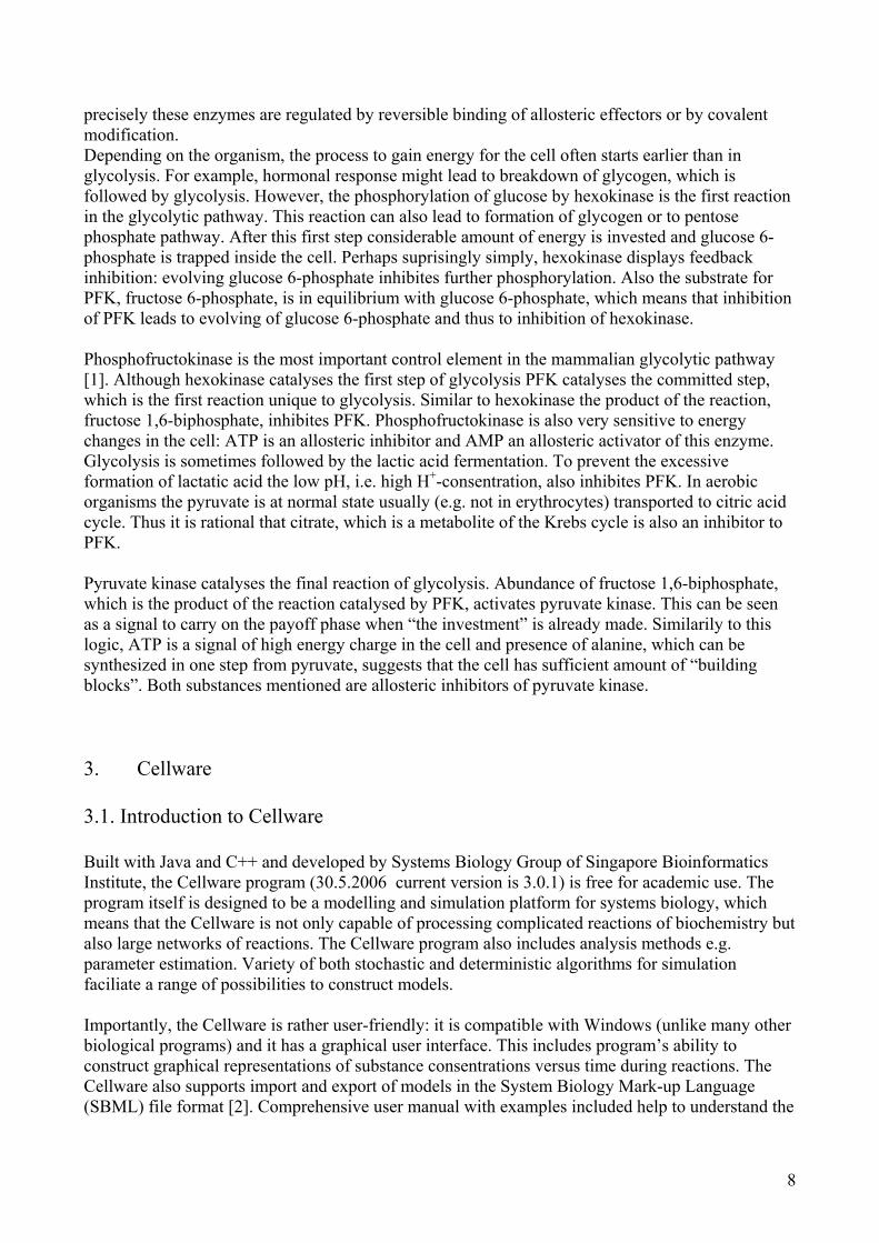
2. Glycolysis 2.1. Introduction to glycolysis Glycolysis is also known as the Embden-Meyerhof pathway named after two German scientists for their research on subject. The essence of this reaction pathway is to create energy for cell’s needs: when one molecule of glucose is converted to two molecules of pyruvate energy is stored in phosphorylation of two molecules of ADP to two molecules of ATP and in reduction of two electron carriers (2 NAD+ + 2e- → 2 NADH). It is important to stress on the fact that glycolysis itself is an anaerobical pathway. In consequence of this one might guess, that glycolysis is ancient in evolutical way. Actually glycolysis was the first metabolic pathway to develop in evolution [3]. In eukaryotes glycolysis takes place in the cytosol. Another point to note is that glycolysis follows quite a forward pattern, unlike e.g. citric acid cycle, which is affected not only by energy charge (energy charge = ([ATP]+(1/2)× [ADP]) / ([ATP]+[ADP]+[AMP])) and pyruvate concentration but also e.g. by fatty acid synthesis (from citrate) and amino acid syntesis (from oxaloacetate). Glycolysis is nearly a straight path. To mention some important exceptions fructose and galactose may enter the reaction pathway: fructose can be phosphorylated to a glycolysis metabolite fructose 6-phosphate by hexokinase, although hexokinase has about 20 times greater affinity for glucose. Galactose can be converted to glucose in four reaciton steps. Also a glycolysis metabolite phosphoenolpyruvate can lead to amino acid synthesis.

Picture one: Simple representation of glycolysis [4]

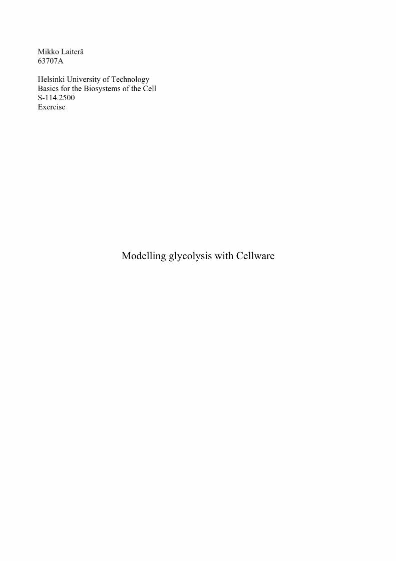
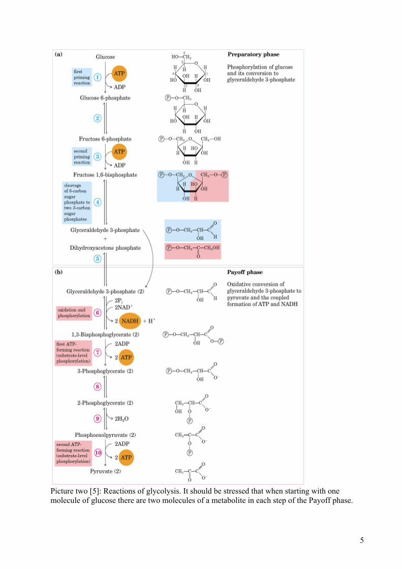
2.2. Reactions and stoichiometry of glycolysis Glycolysis consists of ten reactions and eleven metabolites. Each reaction is catalysed by a different enzyme. The glycolysis can be divided into two or three different phases. A picture of the pathway divided into two phases is shown below. The first phase is called a Preparatory phase, although one might prefer the term “Investing phase” to emphasize the fact that in this first phase energy is spent to gain “profit” later. The second phase is defined here as the “Payoff phase”.

5

Picture two [5]: Reactions of glycolysis. It should be stressed that when starting with one molecule of glucose there are two molecules of a metabolite in each step of the Payoff phase.

6

Overal net reaction of glycolysis is glucose OHHNADHATPpyruvateNADADPPi 222222222 ++++→+++ ++ (2.2.1), where Pi is orthophosphate HPO3

2-, in which the negative charge is delocalised to oxygen atoms. NAD+ is Nicotinamide adenine dinucleotide and can be reduced to NADH by accepting two electrons and a proton. Reaction to gain NADH can be called a ‘hydride transfer’, but it must be kept in mind that electrons of a breaking bond (Highest Occupied Molecular Orbital, HOMO) attack NAD+ (which has Lowest Unoccupied Molecular Orbital, LUMO) and no pure H- occurs in reaction. The most important reactions should be considered a little more in detail. In the first reaction enzyme hexokinase phosphorylates glucose and one ATP is consumed (to ADP). This reaction is notable for three reasons: 1) Hexokinase is one of the regulated enzymes in the pathway, 2) phosphorylation traps glucose in the cell because of two negative charges in glucose 6-phosphate and 3) Phosphorylation destabilizes glucose making way for further catalysis. Third reaction in glycolysis is also a phosphorylation reaction. In this reaction the enzyme phosphofructokinase (PFK) catalyses the phosphorylation of fructose 6-phosphate to fructose 1,6-biphosphate. PFK is the key regulation enzyme in glycolysis and sets the pace of the reaction pathway. An interesting reaction is also fifth reaction of the pathway. It is an isomerization reaction between Dihydroxyacetone phosphate (DAP) and Glyseraldehyde 3-phosphate (GAP) catalysed by enzyme Triose phosphate isomerase (TIM), which is a kinetically perfect enzyme. This means that the speed of catalysis is restricted by diffusion rate rather than by the capasity of the enzyme: TIM accelerates this reaction about 1010-fold. At equilibrium, 96% of the triose phosphate is dihydroxyacetone phosphate [1], but because only GAP can react further in the glycolytic pathway and is thus consumed, the equilibrium is never reached and no DAP is left over. The sixth reaction belongs to the payoff phase. By enzyme Glyseraldehyde 3-phosphate dehydrogenase GAP is converted to 1,3-biphosphoglycerate (1,3-BPG). Actually this reaction consists of four steps (in literature sometimes three, because reduction of NAD+ is not always counted) and has a thioester intermediate. However, the important issue to understand is that this reaction produces a molecule (1,3-BPG) with high phosphoryltransfer potential i.e. a molecule that can phosphorylate ADP to ATP is formed. It should also be noticed that the reaction consists of an oxidising step, where the reaction intermediate is oxidised and NAD+ is reduced to NADH. To maintain the redox equilibrium in a cell the NADH formed must be oxidised later. As maybe easily guessed, in the following reaction (7th) 1,3-BGP phosphorylates one ADP to ATP. The last reaction to mention (10th) is also the last reaction of glycolysis: An another molecule of high phosphorylation potential, phosphoenolpyruvate (PEP), is converted to pyruvate and ATP is formed from ADP. Pyruvate kinase catalyses this reacion and is last (third) enzyme in the reaction pathway subjected to allosteric control. To represent the stoichiometry of glycolysis, the values of thermodynamic equilibrium constants are needed. One should notice the connection between the manner of a reaction and the name of the enzyme catalysing this reaction. If the first reaction in the table has ∆G = -33,5 kJ/mol [1], the equilibrium constant would be 403000/ ≈= ∆− RTG

eq eK , where the molar gas constant KmolJR /3145,8≈ and physiological temperature T = 312.15 K. However in physiological

conditions this value is 250≈eqK [8], i.e. the reaction is not considered irreversible. For an example equilibrium constant values in skeletal muscle tissue are represented are below [1], [3]:

7

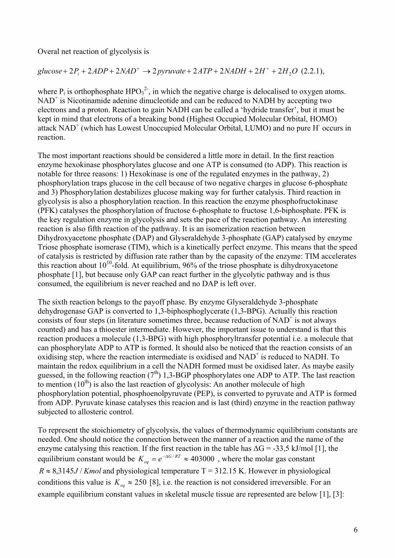
Table one: Stoichiometry of glycolysis in skeletal muscle tissue [1], [3], [8]

Reaction Enzyme ∆G (kJ/mol) in physiological

conditions

Thermodynamic equilibrium

constant 1. Glucose + ATP → glucose 6-phosphate + ADP + H+

Hexokinase -33.5 250

2. Glucose 6-phosphate→ fructose 6-phosphate Phosphoglucose isomerase

-2.5 0.45

3. Fructose 6-phosphate + ATP→ fructose 1,6-biphosphate + ADP + H+

Phosphofructokinase

-22.2 242

4. fructose 1,6-biphosphate→ dihydroxyacetone phosphate + glyseraldehyde 3-phosphate

Aldolase -1.3 9.5 510−×

5. Dihydroxyacetone phosphate→ glyseraldehyde 3-phosphate

Triose phosphate isomerase

+2.5 0.052

6. Glyseraldehyde 3-phosphate + Pi + NAD+ → 1,3-biphosphoglycerate + NADH + H+

Glyceraldehyde 3-phosphate

dehydrogenase

-1.7 0.089

7. 1,3-Biphosphoglycerate + ADP → 3-phosphoglycerate + ATP

Phosphoglycerate kinase

+1.3 57109

8. 3-Phosphoglycerate → 2-phosphoglycerate Phosphoglycerate mutase

+0.8 0.18

9. 2-Phosphoglycerate→ phosphoenolpyruvate + H2O

Enolase -3.3 0.49

10. Phosphoenolpyruvate + ADP + H+→ pyruvate + ATP

Pyruvate kinase -16.4 10304

The product of equilibrium constants is bigger than one, which means that the reaction will proceed “right”. Quantitative analysis of glycolysis will be considered more profoundly in chapter four. 2.3. Regulation of glycolysis The key point in understanding the glycolytic pathway is to recognize the control sites of the pathway i.e. to remember which enzymes are subjected to allosteric regulation and to understand how this is achieved. The activity of glycolysis (or more precisely; its enzymes) is adjusted to meet the energy needs of the cell, but also the need of “building blocks” e.g. for amino acid syntesis. In the reverse pathway, gluconeogenesis, most of the enzymes are same: only the regulatory steps differ. As gluconeogenesis consumes six ATP equivalents (4 ATP, 2 GTP) to convert two molecules of pyruvate to one molecule of glucose, it is essential that the two opposing metabolic pathways do not occur simultaneously (possible exception is brown fat). Powerful regulation also poses a problem for modelling: As some enzymes are allosterically controlled they do not display the Michaelis-Menten kinetics. This means that to construct a sensible model to give meaningful output, lots of research and calculation is needed. Another problem is the import of new glucose into the cell and the consumption of pyruvate. In a model an equilibrium would be reached unlike in real cells. Glycolysis is controlled at three sites. Table one shows that biggest drops in Gibbs free-energy are catalysed by hexokinase, phosphofructokinase and pyruvate kinase respectively. Not suprisingly,

8

precisely these enzymes are regulated by reversible binding of allosteric effectors or by covalent modification. Depending on the organism, the process to gain energy for the cell often starts earlier than in glycolysis. For example, hormonal response might lead to breakdown of glycogen, which is followed by glycolysis. However, the phosphorylation of glucose by hexokinase is the first reaction in the glycolytic pathway. This reaction can also lead to formation of glycogen or to pentose phosphate pathway. After this first step considerable amount of energy is invested and glucose 6-phosphate is trapped inside the cell. Perhaps suprisingly simply, hexokinase displays feedback inhibition: evolving glucose 6-phosphate inhibites further phosphorylation. Also the substrate for PFK, fructose 6-phosphate, is in equilibrium with glucose 6-phosphate, which means that inhibition of PFK leads to evolving of glucose 6-phosphate and thus to inhibition of hexokinase. Phosphofructokinase is the most important control element in the mammalian glycolytic pathway [1]. Although hexokinase catalyses the first step of glycolysis PFK catalyses the committed step, which is the first reaction unique to glycolysis. Similar to hexokinase the product of the reaction, fructose 1,6-biphosphate, inhibites PFK. Phosphofructokinase is also very sensitive to energy changes in the cell: ATP is an allosteric inhibitor and AMP an allosteric activator of this enzyme. Glycolysis is sometimes followed by the lactic acid fermentation. To prevent the excessive formation of lactatic acid the low pH, i.e. high H+-consentration, also inhibites PFK. In aerobic organisms the pyruvate is at normal state usually (e.g. not in erythrocytes) transported to citric acid cycle. Thus it is rational that citrate, which is a metabolite of the Krebs cycle is also an inhibitor to PFK. Pyruvate kinase catalyses the final reaction of glycolysis. Abundance of fructose 1,6-biphosphate, which is the product of the reaction catalysed by PFK, activates pyruvate kinase. This can be seen as a signal to carry on the payoff phase when “the investment” is already made. Similarily to this logic, ATP is a signal of high energy charge in the cell and presence of alanine, which can be synthesized in one step from pyruvate, suggests that the cell has sufficient amount of “building blocks”. Both substances mentioned are allosteric inhibitors of pyruvate kinase. 3. Cellware

3.1. Introduction to Cellware

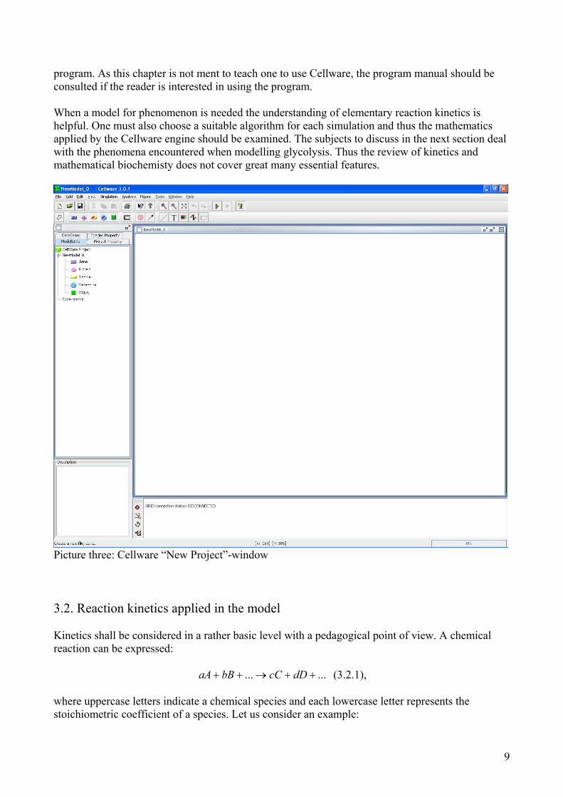
Built with Java and C++ and developed by Systems Biology Group of Singapore Bioinformatics Institute, the Cellware program (30.5.2006 current version is 3.0.1) is free for academic use. The program itself is designed to be a modelling and simulation platform for systems biology, which means that the Cellware is not only capable of processing complicated reactions of biochemistry but also large networks of reactions. The Cellware program also includes analysis methods e.g. parameter estimation. Variety of both stochastic and deterministic algorithms for simulation faciliate a range of possibilities to construct models. Importantly, the Cellware is rather user-friendly: it is compatible with Windows (unlike many other biological programs) and it has a graphical user interface. This includes program’s ability to construct graphical representations of substance consentrations versus time during reactions. The Cellware also supports import and export of models in the System Biology Mark-up Language (SBML) file format [2]. Comprehensive user manual with examples included help to understand the

9

program. As this chapter is not ment to teach one to use Cellware, the program manual should be consulted if the reader is interested in using the program. When a model for phenomenon is needed the understanding of elementary reaction kinetics is helpful. One must also choose a suitable algorithm for each simulation and thus the mathematics applied by the Cellware engine should be examined. The subjects to discuss in the next section deal with the phenomena encountered when modelling glycolysis. Thus the review of kinetics and mathematical biochemisty does not cover great many essential features.

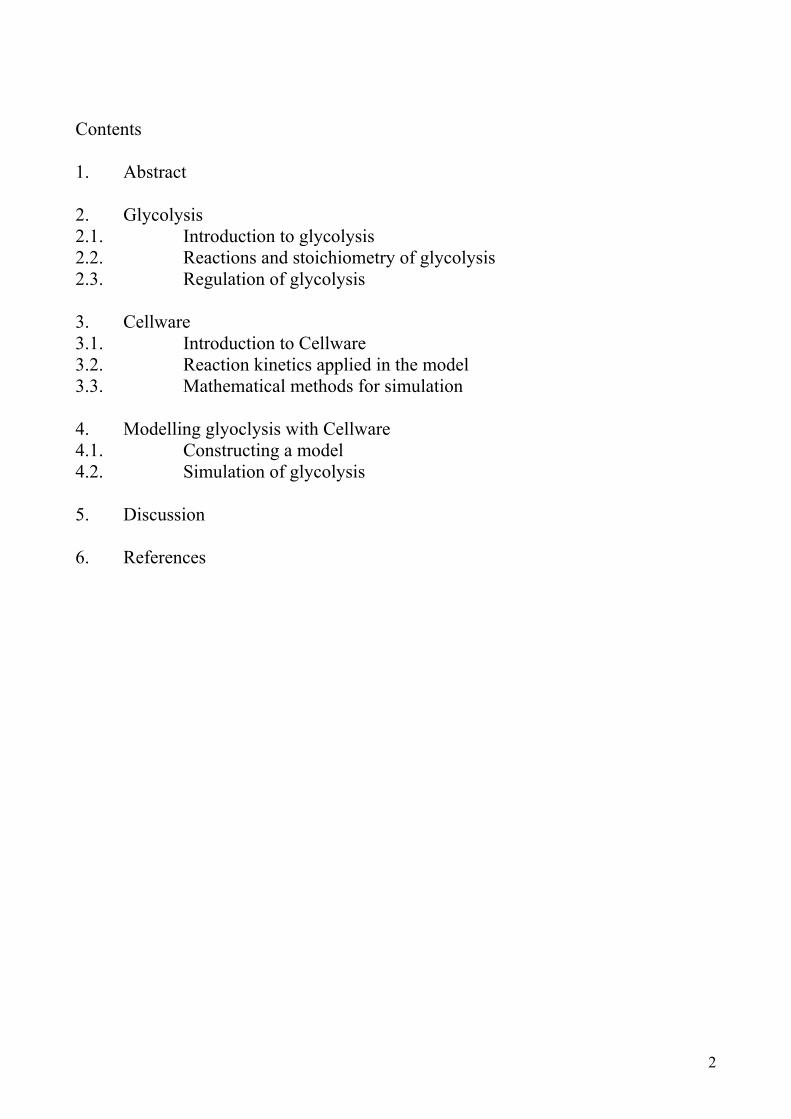
Picture three: Cellware “New Project”-window 3.2. Reaction kinetics applied in the model Kinetics shall be considered in a rather basic level with a pedagogical point of view. A chemical reaction can be expressed:

...... ++→++ dDcCbBaA (3.2.1),

where uppercase letters indicate a chemical species and each lowercase letter represents the stoichiometric coefficient of a species. Let us consider an example:

10

)(2)()(4 5222 gONgOgNO →+ . First and foremost the mass action law states that if a system is at equilibrium at a given temperature, the thermodynamic equilibrium constant

...][][...][][

ba

dc

BADCK = (3.2.2),

where [i] is a concentration of a species i at equilibrium. The example would give

][][][

24

2

252

ONOONK = . An

important relationship, which can derived using laws and definitions of thermodynamics, links the equilibrium constant and the change of Gibbs free energy in reaction:

KRTG ln−=∆ (3.2.3),

where “lnK” is the natural logarithm of the equilibrium constant. Generally during a reaction the number of a species i can be denoted

ξiii vnn += 0 (3.2.4),

where in is the number of moles of species i at any given time durig the reaction, 0in is the number

of moles of a species in the beginning of the reaction, iv is a stoichiometric coefficient of a species i (negative if i is a reactant, positive if i is a product) and ξ is the advancement of the reaction (equal to zero in the beginning). By differentiating both sides from equation (3.2.4) with respect to time is acquired

dtdvdtdn ii // ξ= (3.2.5).

The reaction rate is defined as dtdRate /ξ= . Equation (3.2.5)⇒

dtdnRate ivi/1= (3.2.6).

In the example dtdnRate NO /

241−= but dtdnRate ON /

5221= would do as well.

The problem with equation (3.2.6) is that it depends on the size of the system, i.e. it is an extensive property. The consentration of a species i in a system is )/(][/][ VndidVni =⇒= and thus a more convenient intensive quantity can be used:

dtidVnVRateRii vidt

dv /][)/(/ 11 === (3.2.7).

To define R it was assumed that the volume of the system (V) is independent of time, which is quite logical especially if the time interval is short. So called the rate law is also important. The intensive reaction rate can be written as

11

∏=i

iiAkR α][ (3.2.8),

where k is referred to as the rate constant of the reaction and iα is the reaction order with respect to species Ai. The sum ii

αΣ is called the overall reaction order. This may seem as an easy way to

predict reaction rates but the difficulty is that the parameters αi and k must be determined experimentally. With the example mentioned previously ][][ 2

22 ONOkR = is valid.

The next result shall be used in chapter four. If a reaction reaches an equilibrium, it must have a constant reaction rate also to the reaction from products to reactants. Let the forward rate reaction constant be ka and for opposite direction kb. To simplify matters the forward reaction is first order in A and the back reaction is first order in B: BA ↔ (apologies for wrong type of arrow between A and B). Because of the dynamic equilibrium, ][][/][][][/][ BkAkdtBdBkAkdtAd bABA −==+−= . This can be rearranged to ][2][2 BkAk BA = and finally (kB, [A] ≠ 0) to

KABkk BA == ]/[][/ (3.2.9)

by definition of the equilibrium constant. Thus the equilibrium constant K is linked to reaction kinetics. Quantitative biochemisty consists of a wide range of experimentally derived equations. One of the most important mathematical tools in enzyme kinetics is the Michaelis-Menten equation:

MKSSvv += ][

][max0 (3.2.10),

where v0 is the initial rate of the reaction, vmax is the maximum rate of the reaction, [S] is the substrate consentration and KM is experimentally determined Michaelis constant. To derive this equation so called steady-state conditions must be assumed. This means that even though the concentrations of intermediates of the reaction vary, the concentration of the enzyme-substrate complex is constant [ES]. An other way to put this is that the rates of formation and breakdown of the [ES] complex are equal. It is also assumed that almost no product reverts to the initial substrate. To be precise the allosteric enzymes do not obey Michaelis-Menten equation. However, so-called pseudokinetic rate constants Vmax and Km can be calculated for allosterically controlled enzymes. These constants offer approximate quantification of enzyme kinetics in a narrow predefined substrate consentration interval. 3.3. Mathematical methods for simulation When bioprocesses are simulated, different reactions obeying different kinetics conjugate to form a network of reactions or at least a reaction pathway. One reaction may have an impact on several other reactions and vice versa. These reactions must be written in the language of mathematics if quantitative analysis is needed. Kinetics and thermodynamics provide the means for this. As some variables are unknown and the laws of physics tend to be in a form of differential equations lots of data must be handled in a short time. In addition, most differential equations cannot be solved

12

explicitly and thus numerical methods are needed. This often requires lots of work, i.e. the program must solve many calculations. To reduce this calculation work more efficient algorithms are needed. Developing algorithms, which reduce the number of iterations required or simplify the problem, is a science of its own right. The simulation engine includes two different classes of algorithms, namely the Stochastic Algorithms and Deterministic Algorithms [2]. In addition one hybrid algorithm consisting features from both classes can be chosen. Deterministic algorithms are used when the problem lacks randomnes or it can be ignored. These algorithms are constructed to solve problems that can be formulated using laws of kinetics. These algorithms are convenient for solving problems related to enzyme kinetics and thus they are suitable for simulations of metabolism. The accuracy of the result depends on three things: A function can be “tame”, which means in common language that it doesn’t make rapid turns or have sharp peaks. Some functions are more difficult, and the values of the function and its derivatives may change a lot at some time intervals. Secondly, some numerical methods are simply more effective than others. Finally, the step size is practically the most important factor. The step size is the interval (usually time) between two evaluation points. Thus, the smaller the step size, the smaller the error. Normally one must optimize the method and step size to maximize the accuracy, while maintaining a reasonable simulation time (proportional to calculation work). As most of the differential equations to encounter cannot be solved explicitely the three methods offered in Cellware are all numerical. Actually, giving a “symbolic” result is very difficult for programs as they normally consider numbers as “floats” (floating desimal number). The three possible methods are:

1) Euler forward ode (ode means ordinary differential equation). Euler forward can be considered the most simple algorithm to solve differential equations and is derived below as an example. However, no proof of convergence towards the right solution will be shown. The problem is solved with respect to one variabe. An ODE to solve with respect to time can be formulated

))(,()(' txtftx = , ],0[ Tt ∈ , 0)0( xx = (3.3.1).

The last statement is the initial condition and 0x is a real number. First let q be a continuous function to be solved with respect to time t. If the function q depends also on a set of other variables (e.g. substrate constentration, pH), they can be all represented as one vector y (or if they are equations too a matrix can be used). Now, y has a dimension equivivalent to number of these “other” variables. A continuous function can be represented as its Taylor series:

k

kk

tyq tttyqk

)(),( 00

!),( 0

)(

−= ∑∞

=

(3.3.2),

where 0t is a predefined point for this development (often zero) and ),( 0

)( tyq k means the kth derivative of q with respect to t in 0t . Taylor series always converge (readers interested in proofs should consult literature of analysis), which can be guessed due to rapidly growing divisor k!. Because of this convergense first terms in the serie have greater effect on the sum than the following terms. Thus x of the original ODE (3.3.1) can be approximated by first two terms:

))](([)()( 000 tttxtxtx dtd −+≈ (3.3.3).

13

In numerical methods the time is discreted into steps t0, t0+h, t0+2h,... until the predefined end (e.g. solve consentration after 10s has passed) is reached. The step size is h. To simplify and shorten notations (not the matter!) is assumed t0 =0, i.e time measuring starts at the same time with the simulation. Also in first order differential equations )(txdt

d is known as a function of x and t. Thus it can be referred to as ))(,( txtf . In the explisite Euler method the iterate from previous round is a seed for the next round: )0(0 xx = , which is a known quantity and called an initial condition. The first iterate is

),0())0(,0( 0001 xfxhxfxx +=+= and the second hxhfxx ),( 112 += . Thus the algorithm can be written (k is the number of the iterate).

),(1 kkk xhkhfxx +=+ ,..2,1,0=k (3.3.4).

2) Runge-Kutta 4th order is a classic for an algorithm to solve differential equations. The order

means phases vi calculated per one step. Euler forward is of first order, which suggests that Runge-Kutta 4th must be rather more complicated. However, Runge-Kutta 4th has a local error of factor four (the local error is proportional to fourth power of the step), while Euler forward has a local error of factor one. Runge-Kutta 4th has also better accuracy for calculation work done. Thus Euler forward must be preferred only if the amount of calculation needed is too numerous for Runge-Kutta 4th, although even when dealing with such a massive amount of data should Runge-Kutta 4th with longer step (than for Euler) be considered. No properties for this method is proved here and interested readers should again refer to the literature of analysis. With a common shortening from literature hk = tk and with the similar notations to 1) the algorithm for Runge-Kutta 4th is:

∑

∑

=

+

−

=

+=

++=

=

4

1

1

1

1

1

),,(

),,(

i

ii

kk

i

j

jijkik

i

kk

vbhxx

vahxhctfv

xtfv

i = 2,...,4 (3.3.5)

Thus the phases vi are calculated recursively and the new iterate xk+1 is calculated using phases and the iterate xk from the previous round. The coefficients for Runge-Kutta 4th are c1 = aij = 0, except a21 = a32 = ½ , a43 = 1, b1 = b4 = 1/6 , b2 = b3 = 2/6, c2 = c3 = ½ and c4 = 1.

3) Cellware has also an Advanced ODE Solver for “stiff” ODEs. ODE can be called stiff if it has both tame and difficult sections at chosen time interval. Functions with rapidly changing derivatives require lots of evaluations (calculations) to be made but if a short time step is applied the simulation might take a very long time. Thus stiff ODEs would require short time step, but calculation would take time because of long tame sections of the function. Actually Advanced ODE Solver does not refer to any particular algorithm. Possibly literature has been consulted and an effective algorithm for solving stiff ODEs was chosen. However, this algorithm may have been developed by the Systems Biology Group of Bioinformatics Institute of Singapore itself and it may even be patented. Usually these algorithms for stiff ODEs evaluate derivatives of the function to solve and use shorter time

14

steps when function has rapidly changing derivatives and save calculation time by using longer steps when the function acts “nicely”. Many of such algorithms are somehow based on Runge-Kutta methods.

The Cellware simulation engine includes also stochastic algorithms. Shortly, these algorithms should be used (only), when the simulation consists of random factors. For example, if radioactive decays of a very small quantity of substace are calculated to happen nine times in a minute on average this does not mean (deterministically) that in every minute nine decays take place. Most common situation to require stocastic algorithms is a model dealing with very small consentrations of substances. In these situations the random kinetic energy and movement of single molecules must be considered. Also as a small number of molecules cannot be considered to be evenly distributed, the consentration ceases to be a meaningful quantity to measure. However, glycolysis is a well defined metabolic pathway with sufficiently large consentrations and thus deterministic algorithms are used in the simulation. For this reason stochastic algorithms are not considered further here. A reader interested in stochastic methods of Cellware should refer to its User Manual.

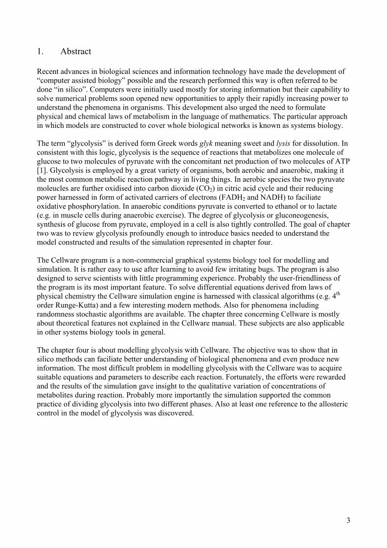
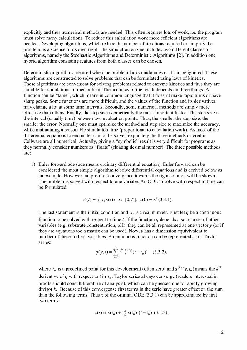
4. Modelling glyoclysis with Cellware 4.1. Constructing a model In the Cellware program “New Project” must be chosen. Then all eleven metabolites can be put on their places. To clarify the model circles representing metabolites are named. Note that the “Caption” of a metabolite cannot contain spaces. Although most properties function fine in version 3.0.1, it is not possible to give a species unique “Full name”. Rather, the program gives always the same name for each species. However, this is quite small a problem as only the “Caption”, which works fine, is shown. Drawing reaction arrows between metabolites (including ATP, NAD, etc.) is a bit messy. Thus the biomolecules, which only accept or lose electrons or an orthophosphate are coloured red as well as the orthophosphate itself. It is essential to remember that in an organism the glycolytic pathway is always followed by reaction(s) to maintain the redox balance, i.e. NADH produced must be oxidised back to NAD+. Thus, in model the amounts of NADH and NAD+ are fixed.

15

Picture four: The arrows indicate whether a metabolite is consumed or produced in reaction. Unfortunately font of the text cannot be changed and thus the names of the metabolites show poorly in picture. 4.2. Simulation of glycolysis Simulation of glycolysis requires initial concentrations of metabolites and kinetic parameter values for reactions. The glycolytic pathway is to be modelled in a yeast cell and suitable kinetics are chosen for each enzyme separately. The program sometimes runs simulations totally wrong if a saved model is opened. Thus the simulation is preferred to be run right after reactions are defined. For reactions including only one substrate and one product the realationship

KABkk BA == ]/[][/ (3.2.9) derived in chapter 3.2. is used. This is done by setting the reverse rate constant one. It should be stressed that this formula is quite approximative as it assumes first order kinetics. For reactions involvig more substrates or products Michaelis-Menten kinetics (3.2.10) or Mass-action kinetics (3.2.8) is used. A slight problem occurred when Cellware refused to apply Michaelis-Menten kinetics for reactions involving more than one substrate or product. The problem was circulated by

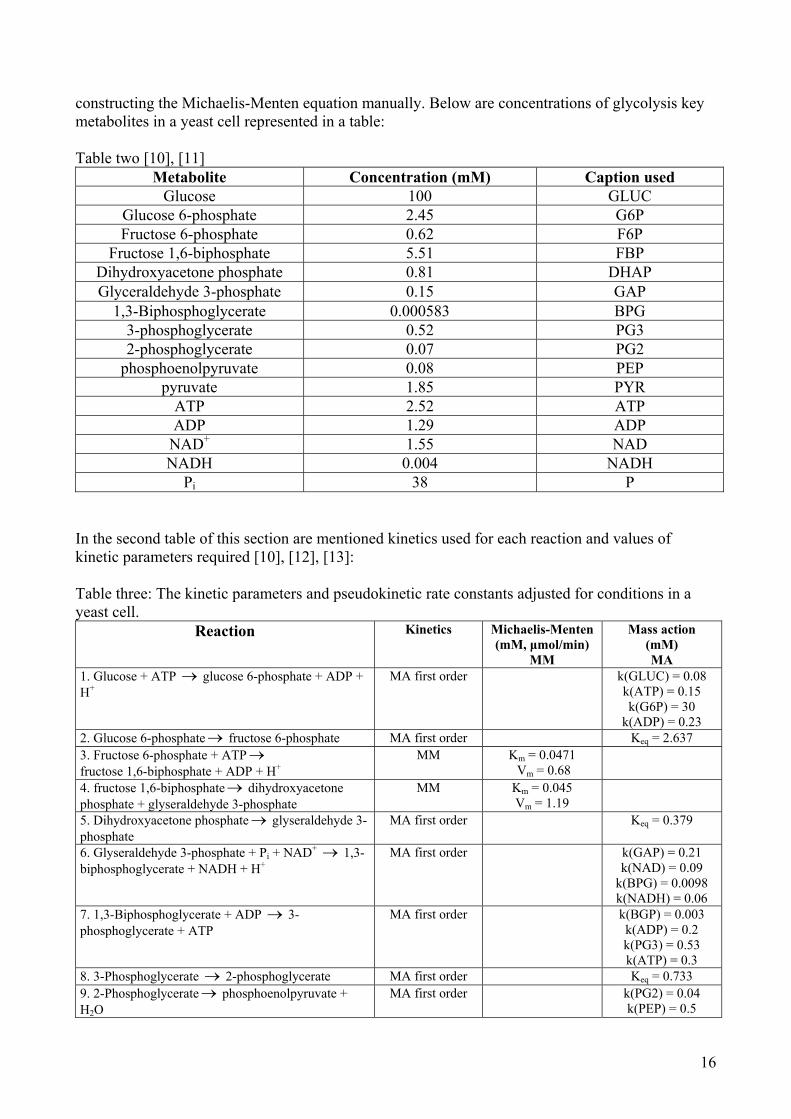
16

constructing the Michaelis-Menten equation manually. Below are concentrations of glycolysis key metabolites in a yeast cell represented in a table: Table two [10], [11]

Metabolite Concentration (mM) Caption used Glucose 100 GLUC

Glucose 6-phosphate 2.45 G6P Fructose 6-phosphate 0.62 F6P

Fructose 1,6-biphosphate 5.51 FBP Dihydroxyacetone phosphate 0.81 DHAP Glyceraldehyde 3-phosphate 0.15 GAP

1,3-Biphosphoglycerate 0.000583 BPG 3-phosphoglycerate 0.52 PG3 2-phosphoglycerate 0.07 PG2

phosphoenolpyruvate 0.08 PEP pyruvate 1.85 PYR

ATP 2.52 ATP ADP 1.29 ADP

NAD+ 1.55 NAD NADH 0.004 NADH

Pi 38 P

In the second table of this section are mentioned kinetics used for each reaction and values of kinetic parameters required [10], [12], [13]:

Table three: The kinetic parameters and pseudokinetic rate constants adjusted for conditions in a yeast cell.

Reaction Kinetics Michaelis-Menten (mM, µmol/min)

MM

Mass action (mM) MA

1. Glucose + ATP → glucose 6-phosphate + ADP + H+

MA first order k(GLUC) = 0.08 k(ATP) = 0.15 k(G6P) = 30

k(ADP) = 0.23 2. Glucose 6-phosphate→ fructose 6-phosphate MA first order Keq = 2.637 3. Fructose 6-phosphate + ATP→ fructose 1,6-biphosphate + ADP + H+

MM Km = 0.0471 Vm = 0.68

4. fructose 1,6-biphosphate→ dihydroxyacetone phosphate + glyseraldehyde 3-phosphate

MM Km = 0.045 Vm = 1.19

5. Dihydroxyacetone phosphate→ glyseraldehyde 3-phosphate

MA first order Keq = 0.379

6. Glyseraldehyde 3-phosphate + Pi + NAD+ → 1,3-biphosphoglycerate + NADH + H+

MA first order k(GAP) = 0.21 k(NAD) = 0.09

k(BPG) = 0.0098 k(NADH) = 0.06

7. 1,3-Biphosphoglycerate + ADP → 3-phosphoglycerate + ATP

MA first order k(BGP) = 0.003 k(ADP) = 0.2 k(PG3) = 0.53 k(ATP) = 0.3

8. 3-Phosphoglycerate → 2-phosphoglycerate MA first order Keq = 0.733 9. 2-Phosphoglycerate→ phosphoenolpyruvate + H2O

MA first order k(PG2) = 0.04 k(PEP) = 0.5

17

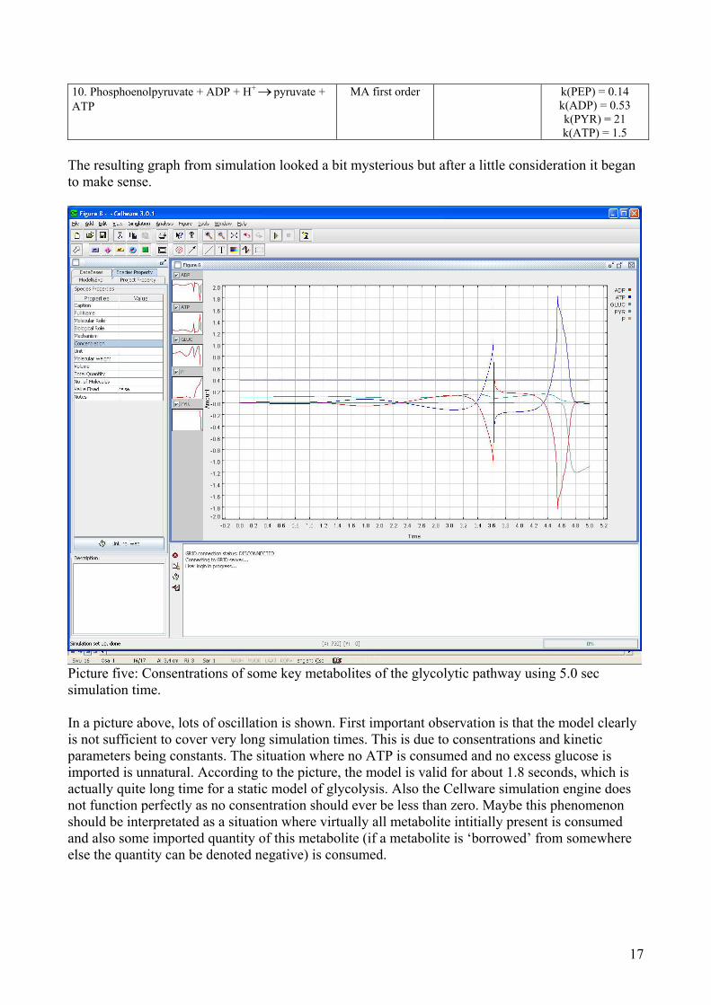
10. Phosphoenolpyruvate + ADP + H+→ pyruvate + ATP

MA first order k(PEP) = 0.14 k(ADP) = 0.53 k(PYR) = 21 k(ATP) = 1.5

The resulting graph from simulation looked a bit mysterious but after a little consideration it began to make sense.

Picture five: Consentrations of some key metabolites of the glycolytic pathway using 5.0 sec simulation time. In a picture above, lots of oscillation is shown. First important observation is that the model clearly is not sufficient to cover very long simulation times. This is due to consentrations and kinetic parameters being constants. The situation where no ATP is consumed and no excess glucose is imported is unnatural. According to the picture, the model is valid for about 1.8 seconds, which is actually quite long time for a static model of glycolysis. Also the Cellware simulation engine does not function perfectly as no consentration should ever be less than zero. Maybe this phenomenon should be interpretated as a situation where virtually all metabolite intitially present is consumed and also some imported quantity of this metabolite (if a metabolite is ‘borrowed’ from somewhere else the quantity can be denoted negative) is consumed.

18

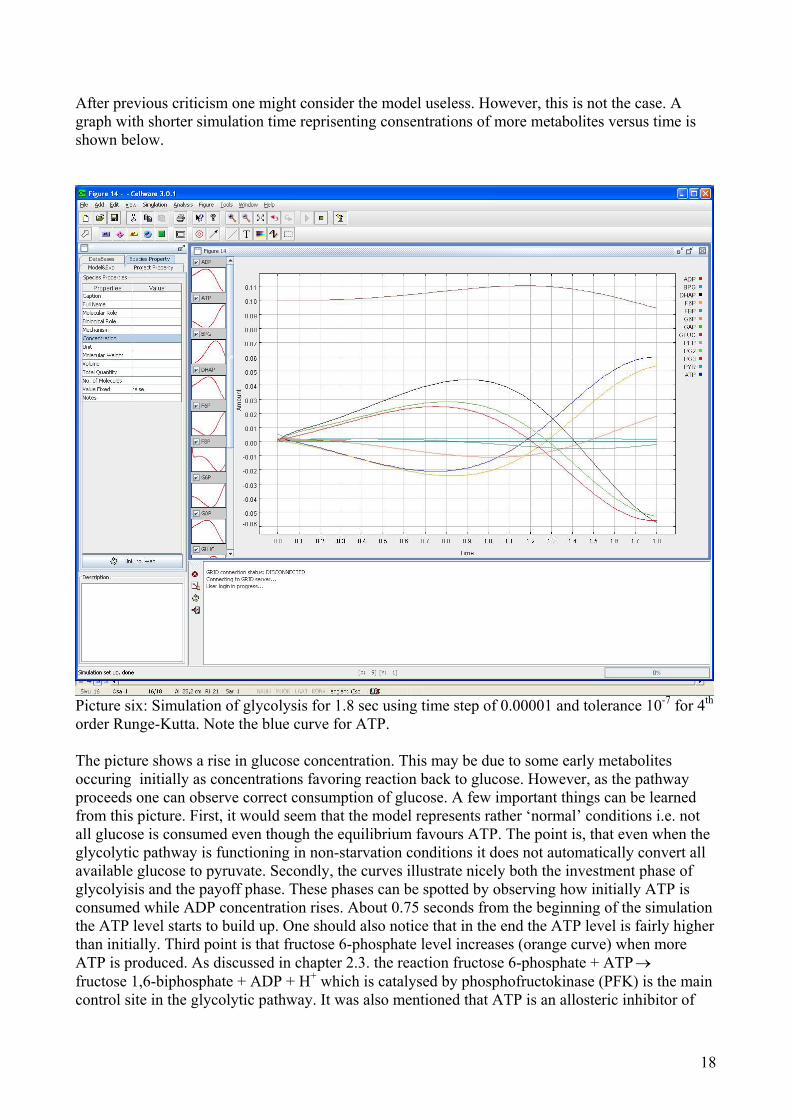
After previous criticism one might consider the model useless. However, this is not the case. A graph with shorter simulation time reprisenting consentrations of more metabolites versus time is shown below.

Picture six: Simulation of glycolysis for 1.8 sec using time step of 0.00001 and tolerance 10-7 for 4th order Runge-Kutta. Note the blue curve for ATP. The picture shows a rise in glucose concentration. This may be due to some early metabolites occuring initially as concentrations favoring reaction back to glucose. However, as the pathway proceeds one can observe correct consumption of glucose. A few important things can be learned from this picture. First, it would seem that the model represents rather ‘normal’ conditions i.e. not all glucose is consumed even though the equilibrium favours ATP. The point is, that even when the glycolytic pathway is functioning in non-starvation conditions it does not automatically convert all available glucose to pyruvate. Secondly, the curves illustrate nicely both the investment phase of glycolyisis and the payoff phase. These phases can be spotted by observing how initially ATP is consumed while ADP concentration rises. About 0.75 seconds from the beginning of the simulation the ATP level starts to build up. One should also notice that in the end the ATP level is fairly higher than initially. Third point is that fructose 6-phosphate level increases (orange curve) when more ATP is produced. As discussed in chapter 2.3. the reaction fructose 6-phosphate + ATP→ fructose 1,6-biphosphate + ADP + H+ which is catalysed by phosphofructokinase (PFK) is the main control site in the glycolytic pathway. It was also mentioned that ATP is an allosteric inhibitor of

19

PFK and as shown in the picture the model actually follows this behaviour: As ATP level increases the PFK is inhibited, which results in rise of fructose 6-phosphate level. Simulations with different initial concentrations would be interesting to analyse. Unfortunately, as stated earlier, the rate constant values are defined for conditions described in table two. Thus if for example initial concentration of glucose were risen significantly the equation for its conversion to glucose 6-phosphate would no longer be valid as the allosterically controlled enzyme hexokinase would then experience rather stronger activation. If one had an acces to kinetic parameters for different conditions the model constructed could be edited. 5. Discussion The exercise consists of three parts: the glycolysis, the Cellware and an integration of these two. The aim was not only to discuss the modelling of glycolysis with Cellware, which the title of the exercise suggests. Such a title as ‘Glycolysis, the Cellware program and simulating glycolysis’ might have been more descriptive but is sounds helplessly dull. The exercise was meant to introduce both glycolysis and the Cellware program for readers not familiar with these concepts. In addition, the goal was to give an example of systems biology in form of simulation of glycolysis and also show that in silico methods can give new insight into biological phenomena. Glycolysis can be studied by reading literature of biochemistry and the Cellware can be learnt from reading the user manual and using the program. However, the simulation run was unique: the results aquired are not borrowed, they were created. The latter sounds rather solemn and one surely realizes that the model described here is just one of the many that can be found on subject. Published scientific articles include more sophisticated and accurate experiments. Anyway, as the modelling can be considered as the most important achievement of this exercise the title is quite justified. Glycolysis is described in chapter two. The text aimed to provide sufficient information for a reader with little experience in biochemistry to understand the logic behind the model constructed and also give insight into the results of the simulation. Also as an understanding of the regulation of the pathway is the key to all kinetic models (or more precisely: defining the kinetic equations and constants) of glycolysis an emphasis is put on this subject. One may have noticed that chapter two actually has adopted a rather systems biological point of view: for example, virtually no information about diseases of malfunctions associating glycolysis is given. Also, even though the structure of biomolecules is an essential factor to their function, no structures of metabolites are discussed. Are these features unimportant? Certainly not, but they are rather irrelevant considering the model applied. After all, the subject was not solely glycolysis. Chapter three is about Cellware. However, as stated earlier the chapter is not a guide to use the program. It is shortly introduced and the methods behind its simulation engine concerning model in chaper four are described. As high school mathematics and chemistry are not sufficient to understand the function of algorithms or most details of kinetics, chapters 3.2. and 3.3. are not as elementary as the chapter two. The difficulty is not intentional, rather it is inevitable. If the basics in solving partial differential equations and physical chemistry were given, the text would be long enough to cover a few books. Anyway, some of the important properties are derived and one good reason to do this was that the Cellware manual simply lists these matters but lacks even the formulas.

20

Description of the modelling in chapter four serves as an example of using the Cellware. However as discussed in this chapter earlier this was not the point. The modelling process including the gathering of suitable reaction equations and constants prooved to be the most challenging task in the exercise. Fortunately, the results acquired were satisfactory and the work was not futile. The meaning of chapter four is analyzed a few times earlier in this chapter. At this point one can self consider the value of the model but a larger issue is the meaning of in silico research in general. With better knowledge and more understanding of different sciences better and better models including large networks of reactions can be constructed. Systems biology can offer methods to lower costs in medicine development, to get more accurate diagnosis for patients and to provide new means to optimize different bioprocesses. The integration of older sciences gives birth to a new branch with potential hard to exaggerate.

21

6. References

[1] J. Berg, J. Tymoczko, L. Stryer: Biochemistry Fifth Edition. W. H. Freeman and Company.

New York. 2002, 423, 436-437, 444, 445 [2] Systems Biology Group, Bioinformatics Institute Singapore: Cellware User Manual, 7, 52 [3] Annals of Biomedical Engineering, Vol 30. M. Lambeth, M. Kushmerick: A Computational

Model for Glycogenolysis in Skeletal Muscle. Biomedical Engineering Society. 2002, 808, 813 [4] Estrella Mountain Community College, Online Biology Book, Mike Farabee, Ph.D.

http://www.emc.maricopa.edu/faculty/farabee/BIOBK/BioBookGlyc.html [5] Eberly College of Science, department of Biochemistry and Molecular Biology. Dr Sypes:

Lecture notes: Glycolysis reactions http://www.bmb.psu.edu/courses/bmb211/classnotes/glycolysisrxns.html

[6] J. Clayden, N. Greeves, S. Warren, P. Wothers: Organic Chemistry. Oxford University Press.

Oxford 2001 [7] T. Engel, P. Reid: Thermodynamics, Statistical Thermodynamics & Kinetics. Pearson

Education, Benjamin Cummings. San Francisco 2005 [8] M. Gregoriou, I. Trayer, A. Cornish-Bowden: Biochemistry 20. 1981. 499-506. [9] Helsinki University of Technology, Laboratory of Mathematics. Timo Eirola:

Osittaisdifferentiaaliyhtälöt, Mat-1.404 Lecture notes spring 2005. [10] European Journal of Biochemistry. 267, 1-18 (2000). B. Teusink et al. Can yeast glycolysis be

understood in terms of in vitro kinetics of the constituent enzymes? Testing biochemistry http://www.bio.vu.nl/hwconf/papers/ca20.pdf

[11] The Walter and Elizia Hall Institute. Melbourne. Australia. A Gottschalk: The Mechanism of

Selective Fermentation of d-Fructose from Invert Sugar by Sauternes Yeast (1946). 624 [12] Beilstein-Institut. Frankfurt. Germany. C. Kettner, M. Hicks: Chaos in the world of enzymes -

How valid is Functional Characterization Without Methodological Experimental data? (2004) http://www.beilstein-institut.de/escec2003/proceedings/Kettner/kettner.htm

[13] European Journal of Biochemistry, Vol 108, 295-301, (1980). F. Gotz, S. Fischer, K. Schleifer:

Purification and characterisation of an unusually heat-stable and acid/base-stable class I fructose 1,6-bisphosphate aldolase from Staphylococcus aureus http://content.febsjournal.org/cgi/content/abstract/108/1/295

22