MULTI-CRITERIA DECISION MAKING WITH INTERDEPENDENT

CRITERIA USING PROSPECT THEORY

A THESIS SUBMITTED TO

THE GRADUATE SCHOOL OF NATURAL AND APPLIED SCIENCES

OF

MIDDLE EAST TECHNICAL UNIVERSITY

BY

AHMET BOZKURT

IN PARTIAL FULFILLMENT OF THE REQUIREMENTS

FOR

THE DEGREE OF MASTER OF SCIENCE

IN

INDUSTRIAL ENGINEERING

JUNE 2007

Approval of the Graduate School of Natural and Applied Sciences

Prof. Dr. Canan ÖZGEN

Director

I certify that this thesis satisfies all the requirements as a thesis for the degree of Master of Science.

Prof. Dr. Çağlar GÜVEN Head of the Department

This is to certify that we have read this thesis and that in our opinion it is fully adequate, in scope and quality, as a thesis for the degree of Master of Science.

Asst. Prof. Dr. Esra KARASAKAL Supervisor

Examining Committee Members Prof. Dr. Gülser Köksal (METU,IE) Asst. Prof. Dr. Esra Karasakal (METU,IE) Assoc. Prof. Dr. Haldun Süral (METU,IE) Asst. Prof. Dr. Seçil Savaşaneril (METU,IE) Dr. Orhan Karasakal (Turkish Navy)

iii

I hereby declare that all information in this document has been obtained and

presented in accordance with academic rules and ethical conduct. I also

declare that, as required by these rules and conduct, I have fully cited and

referenced all material and results that are not original to this work.

Ahmet BOZKURT

iv

ABSTRACT

MULTI-CRITERIA DECISION MAKING WITH INTERDEPENDENT

CRITERIA USING PROSPECT THEORY

Bozkurt, Ahmet

M. Sc., Department of Industrial Engineering

Supervisor: Asst. Prof. Dr. Esra KARASAKAL

June 2007, 102 pages

In this study, an integrated solution methodology for a general discrete multi-

criteria decision making problem is developed based on the well-known outranking

method Promethee II. While the methodology handles the existence of

interdependency between the criteria, it can also incorporate the prospect theory in

order to correctly reflect the decision behavior of the decision maker. A software is

also developed for the application of the methodology and some applications are

performed and presented.

Keywords: Multiple Criteria Decision Making, Interdependency among Criteria,

Prospect Theory

v

ÖZ

TERCİH TEORİSİ KULLANARAK BAĞIMLI KRİTERLERİN OLDUĞU

DURUMDA ÇOK KRİTERLİ KARAR VERME

Bozkurt, Ahmet

Yüksek Lisans, Endüstri Mühendisliği Bölümü

Tez Yöneticisi: Yard. Doç. Dr. Esra KARASAKAL

Haziran 2007, 102 sayfa

Bu çalışmada en çok bilinen çok kriterli karar verme yöntemlerinden biri olan

Promethee yöntemi baz alınarak melez bir sıralama metodolojisi geliştirilmiştir.

Geliştirilen yöntem kriter ağırlıklarının hesaplanmasında kriterler arasındaki

etkileşimin etkisini yansıtabilmesinin yanısıra karar vericinin karar vermede

gösterdiği yaklaşımın sonuçlara etkisini de hesaplamada kullanabilmektedir. Ayrıca

geliştirilen yöntemin uygulanmasında kullanılmak üzere bir yazılım da

geliştirilmiştir. Bu yazılım kullanılarak yapılan örnek uygulamalar da tez

kapsamında sunulmuştur.

Anahtar Kelimeler: Çok Kriterli Karar Verme, Kriterler Arası Bağımlılık, Tercih

Teorisi

vi

ACKNOWLEDGEMENTS

I would like to express my deepest gratitude to all my instructors in Industrial

Engineering Department, and especially to my supervisor, Assist. Prof. Dr. Esra

Karasakal, for her continuous guidance, encouragement and both academic and

personal support throughout my thesis study.

I also thank my friends, especially my colleague M. Ural Uluer for making the

thesis period enjoyable and colorful and Cihan Selçuk for his invaluable support

during the programming stage.

Also, for and beyond this thesis study, I am indebted to my family (Murat, Elmas,

Cansu, Zeynep, Bahar and İbrahim) for their continuous love and belief and their

patience throughout my academic life.

Finally, for being always there with me during the study with her never ending

support, I thank to my dear love Sevil.

vii

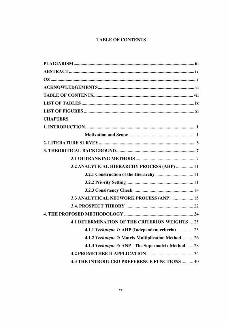
TABLE OF CONTENTS

PLAGIARISM......................................................................................................... iii

ABSTRACT............................................................................................................. iv

ÖZ.............................................................................................................................. v

ACKNOWLEDGEMENTS.................................................................................... vi

TABLE OF CONTENTS....................................................................................... vii

LIST OF TABLES .................................................................................................. ix

LIST OF FIGURES ................................................................................................ xi

CHAPTERS

1. INTRODUCTION................................................................................................ 1

Motivation and Scope .......................................................... 1

2. LITERATURE SURVEY.................................................................................... 3

3. THEORITICAL BACKGROUND..................................................................... 7

3.1 OUTRANKING METHODS .................................................... 7

3.2 ANALYTICAL HIERARCHY PROCESS (AHP) ............... 11

3.2.1 Construction of the Hierarchy ................................. 11

3.2.2 Priority Setting .......................................................... 11

3.2.3 Consistency Check .................................................... 14

3.3 ANALYTICAL NETWORK PROCESS (ANP) ................... 15

3.4. PROSPECT THEORY ........................................................... 22

4. THE PROPOSED METHODOLOGY ............................................................ 24

4.1 DETERMINATION OF THE CRITERION WEIGHTS .... 25

4.1.1 Technique 1: AHP (Independent criteria)............... 25

4.1.2 Technique 2: Matrix Multiplication Method .......... 26

4.1.3 Technique 3: ANP - The Supermatrix Method ...... 28

4.2 PROMETHEE II APPLICATION......................................... 34

4.3 THE INTRODUCED PREFERENCE FUNCTIONS .......... 40

viii

4.3.1 Preference Function VII (Linear criterion with

indifference threshold area) .............................................. 41

4.3.2 Preference Function VIII (Exponential Function

with Indifference Area)...................................................... 42

5. THE SOFTWARE ............................................................................................. 45

6. COMPARISON OF THE WEIGHT DETERMINATION TECHNIQUES 52

7. SAMPLE SOLUTIONS..................................................................................... 58

7.1 ORIGINAL PROBLEM.......................................................... 59

7.2 GENERATED SCENARIOS FOR SAMPLE SOLUTIONS65

7.2.1 Scenario I ................................................................... 65

7.2.2 Scenario II.................................................................. 67

7.2.3 Scenario III ................................................................ 70

7.2.4 Scenario IV ................................................................ 71

7.2.5 Scenario V .................................................................. 72

7.3 SUMMARY AND DISCUSSION ........................................... 73

8. SAMPLE APPLICATION: RANKING THE UNIVERSITIES ................... 76

8.1 THE ORIGINAL RANKING STUDY................................... 76

8.2 RANKING USING THE METHODOLOGY ....................... 80

8.2.1 Scenario I ................................................................... 80

8.2.2 Scenario II.................................................................. 81

8.2.3 Scenario III ................................................................ 82

8.3 COMPARISONS...................................................................... 83

CONCLUSION....................................................................................................... 85

REFERENCES....................................................................................................... 88

APPENDICES ........................................................................................................ 96

A. APPLICATION: RANKING THE UNIVERSITIES ............ 96

A.1 Problem Data (6 criteria, 101 alternatives)............... 96

A.2 Data Sources ................................................................ 99

A.3 Rankings for the top 101 universities around the

world.................................................................................. 100

ix

LIST OF TABLES

TABLES

Table 3.1 Preference relations used in outranking methods...................................... 7

Table 3.2 Interpretation of Saaty`s 1 – 9 scale ........................................................ 12

Table 3.3 Random consistency indices ................................................................... 15

Table 6.1 Sample results from a 3 criteria case....................................................... 53

Table 6.2 Average deviations from the original weights ........................................ 54

Table 6.3 The weighted supermatrix for ANP(w1, w2) application ........................ 55

Table 6.4 Solutions with AHP, Matrix Mult. & ANP techniques........................... 57

Table 7.1 Criteria of the sample problem................................................................ 61

Table 7.2 Alternatives of the original problem (Wang et al.) ................................. 61

Table 7.3 The square matrix (AHP) for weight determination (Wang et al.) ......... 62

Table 7.4 The evaluation matrix of the original problem (Wang et al.).................. 64

Table 7.5 Preference functions and the corresponding parameters......................... 64

Table 7.6 Promethee flows of the original problem................................................ 65

Table 7.7 Impact Matrix (Interrelationships among criteria) .................................. 66

Table 7.8 Weights deviations (Technique 2, Matrix Mult.) .................................... 66

Table 7.9 Promethee flows for the scenario I.......................................................... 67

Table 7.10 The weighted supermatrix for ANP application (Scenario II) .............. 68

Table 7.11 Weights deviations (Technique 3, ANP(0.5,0.5)) ................................. 69

Table 7.12 Promethee flows for the scenario II ...................................................... 69

Table 7.13 Preference functions and the parameters (Scenario III) ........................ 70

Table 7.14 Promethee flows for the scenario III ..................................................... 71

Table 7.15 Promethee flows for the scenario IV..................................................... 72

Table 7.16 Promethee flows for the scenario V ...................................................... 73

Table 7.17 Summary: Weights Net Flows and Final Rankings .............................. 75

Table 8.1 Criteria definitions & weights of the original study................................ 79

Table 8.2 Preference functions and the parameters (Scenario II & III) .................. 80

x

Table 8.3 The weighted supermatrix for ANP application (Scenario II) ................ 82

Table 8.4 Ranking deviations among the scenarios ................................................ 84

Table A.1 Criteria values for the alternatives.......................................................... 96

Table A.2 Rankings obtained ................................................................................ 100

xi

LIST OF FIGURES

FIGURES

Figure 3.1 Square matrix......................................................................................... 12

Figure 3.2 (a) Linear hierarchy and (b) nonlinear network. (Wey et al., 2006)...... 16

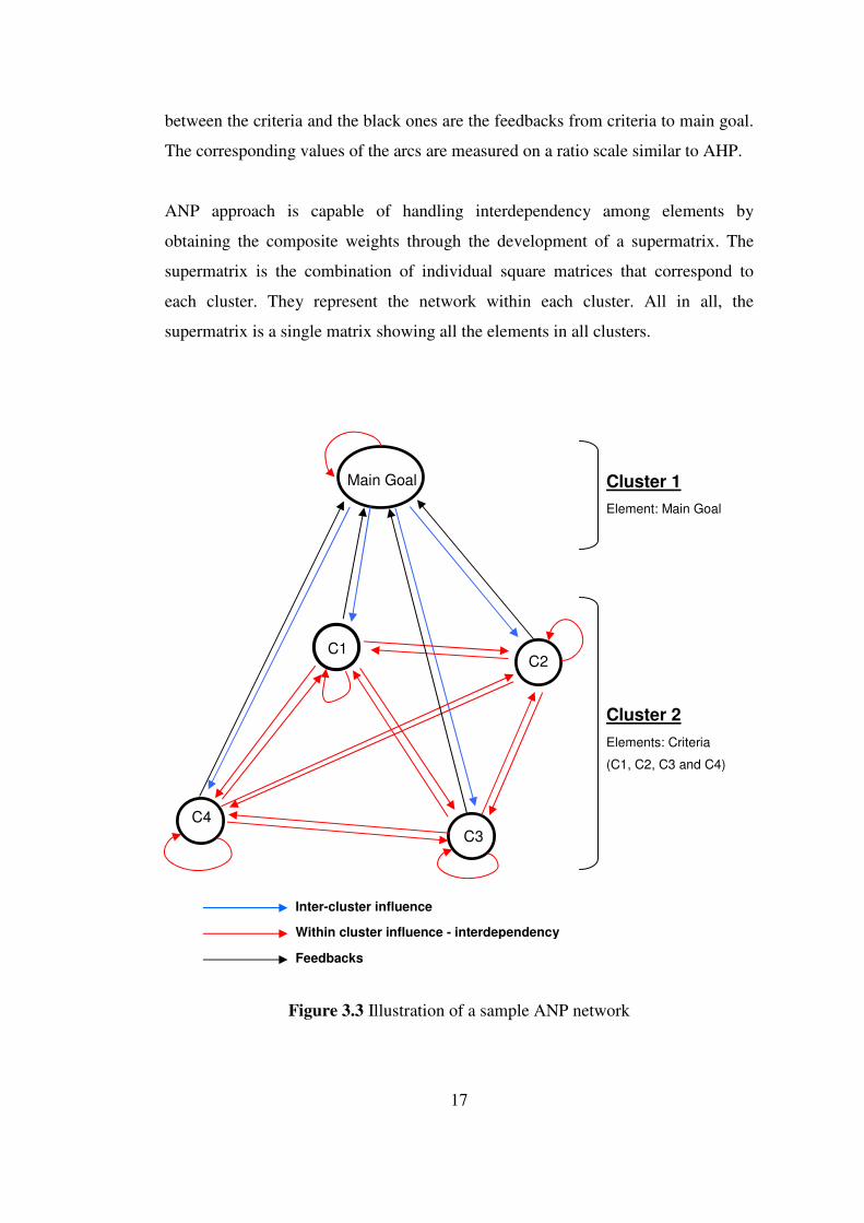
Figure 3.3 Illustration of a sample ANP network ................................................... 17

Figure 3.4 The supermatrix ..................................................................................... 19

Figure 3.5 General preference function according to Prospect Theory .................. 22

Figure 4.1 The criteria comparison matrix w.r.t. criteria i ...................................... 26

Figure 4.2 The impact matrix.................................................................................. 27

Figure 4.3 (a) The conventional and (b) the reduced problem structure................. 28

Figure 4.4 The conventional and the reduced supermatrix ..................................... 29

Figure 4.5 Regions of the reduced supermatrix and interpretations ....................... 31

Figure 3.6 Preference Functions, Brans et al. (1986).............................................. 36

Figure 3.7 The introduced preference functions reflecting the Prospect Theory.... 37

Figure 4.8 Preference indices table (Π1) and calculation of leaving flows, ........... 39

Figure 4.9 Preference indices table (Π2) and calculation of entering flows, .......... 39

Figure 4.10 Linear criterion with indifference threshold area (Prospect Theory) .. 42

Figure 4.11 Exponential function with indifference area (Prospect Theory).......... 44

Figure 5.1 The opening window: Problem definition stage .................................... 46

Figure 5.2 Pairwise comparison window ................................................................ 47

Figure 5.3 Specifying the cluster weights ............................................................... 47

Figure 5.4 Evaluation window ................................................................................ 49

Figure 5.5 The final window: Outranking degrees, Promethee flows & final ranking

.......................................................................................................................... 50

Figure 5.6 The algorithm of the software................................................................ 51

Figure 6.1 Weights obtained for a 3-Criteria case .................................................. 53

Figure 6.2 Network for the ANP(w1, w2) application............................................. 56

Figure 6.3 Variation of the weights with alt. techniques ........................................ 57

xii

Figure 7.1 The hierarchy of the sample problem (Wang et al.) .............................. 62

Figure 7.2 Complete ranking of alternatives (Original solution, Wang et al.)........ 65

Figure 7.3 Complete ranking of alternatives (Scenario I)....................................... 67

Figure 7.4 Complete ranking of alternatives (Scenario II)...................................... 69

Figure 7.5 Complete ranking of alternatives (Scenario III) .................................... 71

Figure 7.5 Complete ranking of alternatives (Scenario IV) .................................... 72

Figure 7.6 Complete ranking of alternatives (Scenario V) ..................................... 72

1

CHAPTER 1

INTRODUCTION

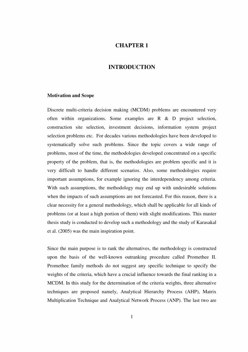
Motivation and Scope

Discrete multi-criteria decision making (MCDM) problems are encountered very

often within organizations. Some examples are R & D project selection,

construction site selection, investment decisions, information system project

selection problems etc. For decades various methodologies have been developed to

systematically solve such problems. Since the topic covers a wide range of

problems, most of the time, the methodologies developed concentrated on a specific

property of the problem, that is, the methodologies are problem specific and it is

very difficult to handle different scenarios. Also, some methodologies require

important assumptions, for example ignoring the interdependency among criteria.

With such assumptions, the methodology may end up with undesirable solutions

when the impacts of such assumptions are not forecasted. For this reason, there is a

clear necessity for a general methodology, which shall be applicable for all kinds of

problems (or at least a high portion of them) with slight modifications. This master

thesis study is conducted to develop such a methodology and the study of Karasakal

et al. (2005) was the main inspiration point.

Since the main purpose is to rank the alternatives, the methodology is constructed

upon the basis of the well-known outranking procedure called Promethee II.

Promethee family methods do not suggest any specific technique to specify the

weights of the criteria, which have a crucial influence towards the final ranking in a

MCDM. In this study for the determination of the criteria weights, three alternative

techniques are proposed namely, Analytical Hierarchy Process (AHP), Matrix

Multiplication Technique and Analytical Network Process (ANP). The last two are

2

suggested for the case of interdependency and feedback among the elements of the

problem, which are important issues for MCDM problems. In literature, generally

the criteria are assumed to be independent of each other, which is not the case most

often however. For example, while deciding upon choosing which projects to

follow, time duration that will elapse and the overall cost of the project can not be

treated independently.

On the other hand, though it is proved with studies that prospect theory models the

choice behavior of the decision maker more accurately, not many studies have been

conducted to implement it into MCDM problems. Besides the classical preference

functions proposed with Promethee family methods, functions representing the

decision behavior of the decision maker in accordance with the prospect theory are

also proposed in the methodology developed in this study.

Organization of the rest of the thesis is as follows: In the second chapter of this

study, the literature survey about the topic and the related studies are presented. In

chapter three, theoretical background about the techniques and methods that are

utilized throughout the development of the methodology is given. Afterwards in

chapter four the development of the methodology is described in detail. Chapter

five introduces the software developed by explaining the user interfaces with an

example application. A study conducted for the comparison of the weight

determination techniques is presented in chapter six whereas in chapter seven and

eight sample problems and their variations are solved and the final rankings are

compared.

3

CHAPTER 2

LITERATURE SURVEY

In the context of discrete MCDM problems, many methodologies have been

developed and proposed, utilizing numerous numerical and empirical methods.

Analytical Hierarchy Process (AHP), developed by Thomas L. Saaty (1980), is one

of the most popular techniques used by the researchers and practitioners. It is a

pairwise comparison technique, which can model the complex problems in a

unidirectional hierarchal structure assuming that there are no interdependencies

between or within the levels. It is a relatively simple and intuitive tool, which

allows the conversion of qualitative values into the quantitative ones. Some

examples of the AHP applications in literature are as follows: Jain et al. (1996) uses

simply AHP for a new venture selection problem, where both quantitative and

qualitative values are easily handled. Khalil et al. (2002) used AHP to select the

appropriate project delivery method. AHP is again used to assign proper weights in

a 0-1 goal programming application by Kwak et al. (1997). Moreover, Gabriel et al.

(2005) utilized AHP and Monte Carlo simulation when the data is uncertain.

Tavana (2003) incorporated group decision making with AHP for evaluating and

prioritizing advanced technology projects at NASA. In their study, Ramachandran

et al. (2004) searched the applicability of AHP for sustainable energy policy

decisions.

Saaty et al. (1986) revised AHP in their study so that it can handle the non-linear

hierarchies. Saaty (1996) then developed the Analytical Network Process (ANP),

which is a general form of AHP. Upon the beneficial properties of AHP, ANP can

handle interdependence and feedback and reveals the composite weights through

the calculations using the supermatrix phenomena. Ulutaş (2005) applied ANP to

evaluate the alternative energy sources for the country. ANP is utilized for R & D

4

project selection in a study by Meade et al. (2002). Cheng et al. (2007) re-solved the

project selection problem, stating the errors made by Meade et al. They again

studied the application of ANP in process models with an example on making

decisions regarding strategic partnering. Shyur et al. (2005) used ANP during the

development of a hybrid method where interdependency among criteria exists.

Jarkharia et al. (2005) solved the problem of logistics service provider with an ANP

application. Wey et al. (2007) used 0-1 goal programming together with ANP for a

resource allocation problem in transportation infrastructure.

While ANP is a practical tool for handling interdependencies among the criteria,

which is the main concern of this study, some other techniques are also developed

for this purpose. For example, Karasakal et al. (2005) proposed a technique

utilizing the “impact matrix” concept and the matrix multiplication operation in

order to obtain the composite weights of the criteria. Carlsson et al. (1994)

introduced interdependency concept into MCDM. Their suggestions are built upon

three types of relationships between criteria, which are support, conflict and

independency. They illustrated the technique with a numerical example. Later on,

Östermark (1996) improved their technique. Preemptive Goal Programming

technique is used in the study of Santhanam et al. (1994). They formed a multi-

criteria model for solving an Information System project selection problem with

interdependencies.

Another useful tool for solving discrete MCDM problems is Preference Ranking

Organization METHod for Enrichment Evaluations (PROMETHEE), a new class of

outranking methods developed by Brans et. al. (1985). Using these methods, either

a partial preorder (Promethee I) or a complete preorder (Promethee II) of all the

alternatives can be proposed to the decision maker(s). Only a few parameters are

asked to the decision maker(s), and they are easy to understand since they have an

economic signification. Another Promethee Family method is Promethee V,

introduced by Brans et al. (1992). With this method, a number of constraints are

incorporated to the alternatives and the problem is converted to a 0-1 goal

5

programming problem. This method is useful for resource allocation and project

ranking-selection type of problems. Abu-Taleb et al. (1995) used Promethee V for a

water resources planning problem in Middle East. Later Mavrotas et al. (2006)

improved the Promethee V application of Abu-Taleb et al. (1995) with a project

prioritization application.

AHP and PROMETHEE methods are analyzed and discussed together thoroughly

in the study of Macharis et al. (2004). They state that operational synergies could be

achieved by integrating Promethee and a number of elements associated with AHP.

More specifically, they argue that AHP could be used during the weight

determination stage of Promethee method, in which no particular weighing

approach was suggested. Similarly, Wang et al. (2006) combined AHP and

Promethee II to form a hybrid method to rank alternatives. They used AHP for

determination of the weights of the criteria and to understand the structure of the

problem whereas Promethee II for the final ranking. Similarly, Babic et al. (1996)

used Promethee II together with AHP to specify the priorities of the criteria in a

MCDM problem.

Besides using AHP-Promethee pair, there are also some other studies to develop

hybrid methodologies which are the combinations of the unique and specific tools.

For example, Lee et al. (2001) proposes an integrated approach for solving

interdependent multi-criteria IS project selection problems using Delphi, ANP and

0-1 GP. In their study, ANP is used for weight determination of the criteria, since

interdependencies exist between criteria.

Choice behavior of the decision maker is another issue that is concerned in this

study. Keeney and Raiffa (1976) used Multi-Attribute Utility Theory (MAUT) to

model the choice behavior of the DM for each criterion and evaluated the overall

utility of each alternative for the DM by either additive or multiplicative utility

function. The alternatives are then ranked according to the final utilities. However,

it is commonly accepted that MAUT fails to reflect the actual choice behavior of the

6

decision maker. Kahneman and Tversky (1979) came up with a new theory called

Prospect theory, stating that the outcomes are expressed as positive or negative

deviations (gains or losses) from a reference alternative or aspiration level and

losses have higher impact than the gains. Currim et al. (1989) showed in their study

that prospect theory “outperforms” utility theory for paradoxical choices.

Although researches, experiments and empirical studies prove that Prospect Theory

better models the choice behavior, there are few studies in literature about

applications within the context of MCDM. Though it was originally developed for

single criterion problems, the ideas have been extended to MCDM problems as well

by Korhonen et al. (1990). They conducted an experimental study to observe the

choice behavior and their results were persistent with Prospect Theory. Salminen

(1994) also incorporated the prospect theory to MCDM. In his study, piecewise

linear marginal value functions are assumed to approximate the S-shaped value

functions of prospect theory. Another study conducted by Karasakal et al. (2005)

integrated the Prospect Theory into Promethee. They have adopted the weights

associated with the criteria for the imprecise information situation through an

interactive procedure with the decision maker.

This study incorporates the basic tools of MCDM to develop a ranking

methodology. These tools are namely Promethee II method, AHP & ANP and

Prospect theory.

Another method very often used to solve discrete MCDM problems is Data

Envelopment Analysis (DEA), Cook et al. (2000) applied DEA for a project

prioritization problem. In their study, evaluation and selection are combined in a

single model by placing the DEA model within a mixed-binary linear programming

context. Green et al. (1995) uses again DEA, where besides using each alternative’s

rating of itself, they also make use of each alternative’s ratings of all the alternatives

through a cross-evaluation concept.

7

CHAPTER 3

THEORITICAL BACKGROUNG

3.1 OUTRANKING METHODS

Ranking of alternatives is encountered very often in the MCDM type of problems.

Outranking methods are utilized in order to derive a solution to such problems.

They provide either weaker or poorer models than the utility function method;

however, they are built upon fewer assumptions and require less effort, which

makes these methods very popular and easily applicable indeed.

Outranking methods are based on pairwise comparison of possible alternatives

along each criterion. The preference relations used for the pairwise comparisons are

given in Table 3.1.

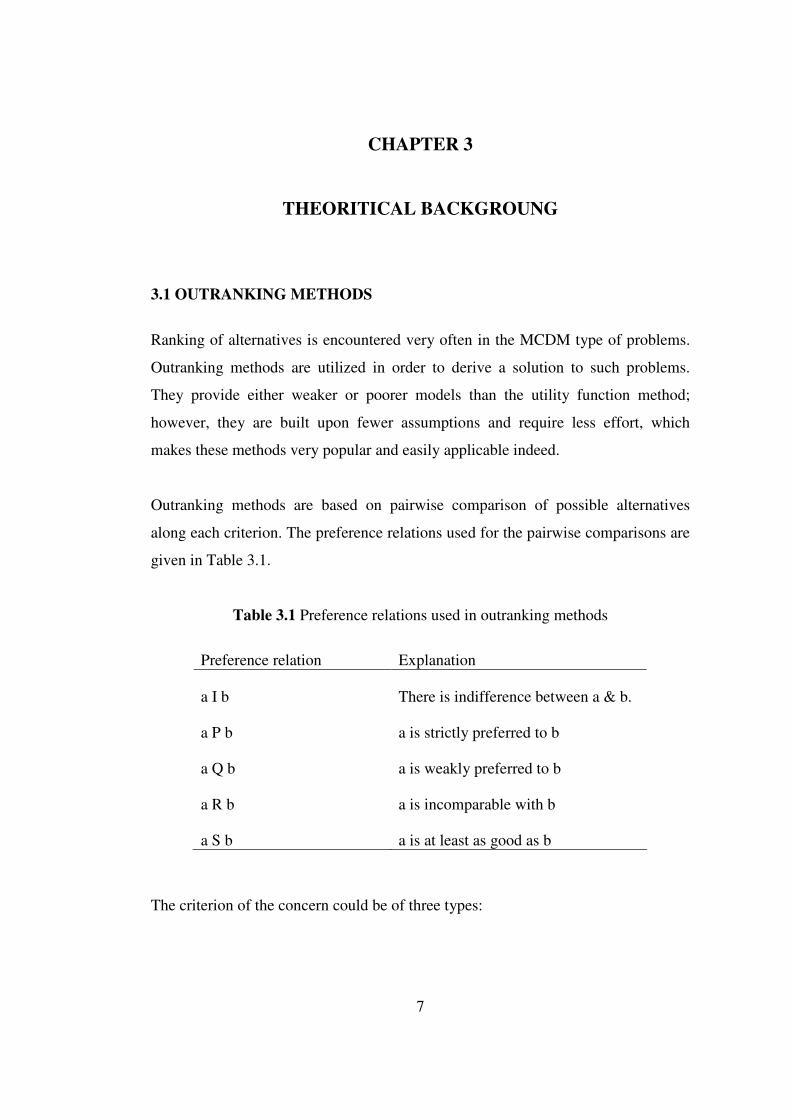
Table 3.1 Preference relations used in outranking methods

Preference relation Explanation

a I b There is indifference between a & b.

a P b a is strictly preferred to b

a Q b a is weakly preferred to b

a R b a is incomparable with b

a S b a is at least as good as b

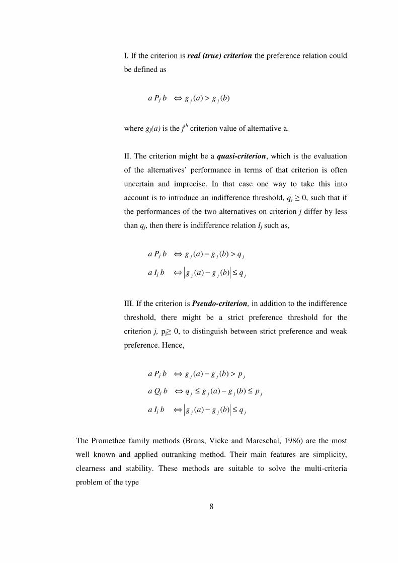
The criterion of the concern could be of three types:

8

I. If the criterion is real (true) criterion the preference relation could

be defined as

a Pj b )()( bgag jj >⇔

where gj(a) is the jth criterion value of alternative a.

II. The criterion might be a quasi-criterion, which is the evaluation

of the alternatives’ performance in terms of that criterion is often

uncertain and imprecise. In that case one way to take this into

account is to introduce an indifference threshold, qj ≥ 0, such that if

the performances of the two alternatives on criterion j differ by less

than qj, then there is indifference relation Ij such as,

a Pj b jjj qbgag >−⇔ )()(

a Ij b jjj qbgag ≤−⇔ )()(

III. If the criterion is Pseudo-criterion, in addition to the indifference

threshold, there might be a strict preference threshold for the

criterion j, pj≥ 0, to distinguish between strict preference and weak

preference. Hence,

a Pj b jjj pbgag >−⇔ )()(

a Qj b jjjj pbgagq ≤−≤⇔ )()(

a Ij b jjj qbgag ≤−⇔ )()(

The Promethee family methods (Brans, Vicke and Mareschal, 1986) are the most

well known and applied outranking method. Their main features are simplicity,

clearness and stability. These methods are suitable to solve the multi-criteria

problem of the type

9

{ }KaafafMax n ∈)(),...,(1

where K is a finite set of alternatives and fi, i = 1,…,n, are n criteria to be

maximized.

The method is based on the pairwise comparison of alternatives with respect to each

criterion according to a valued outranking relation which belongs to that criterion.

There is a weak assumption of preferential independence among the criteria in the

Promethee methods, i.e., it is assumed that the criterion values has no influence on

the preference function of another criterion. First the type of each criterion

(preference function) and -if necessary- the corresponding parameter(s) are defined

at the beginning of the decision process with the decision maker(s). The decision

maker is asked only for a few parameters, which all have an economic significance

so that the decision maker is able to determine their values intuitively.

The weights can be determined using various methods, and the overview of these

methods are listed and analyzed in the study of Nijkamp et al. (1990). Promethee

family methods do not provide specific guidelines for determining these weights,

but assumes that the decision maker is able to assign weight to each criterion

appropriately, at least when the number of the criteria is not large. In this study, the

determination of the weights of the criteria covered extensively and alternative

methods are presented in chapter 4.

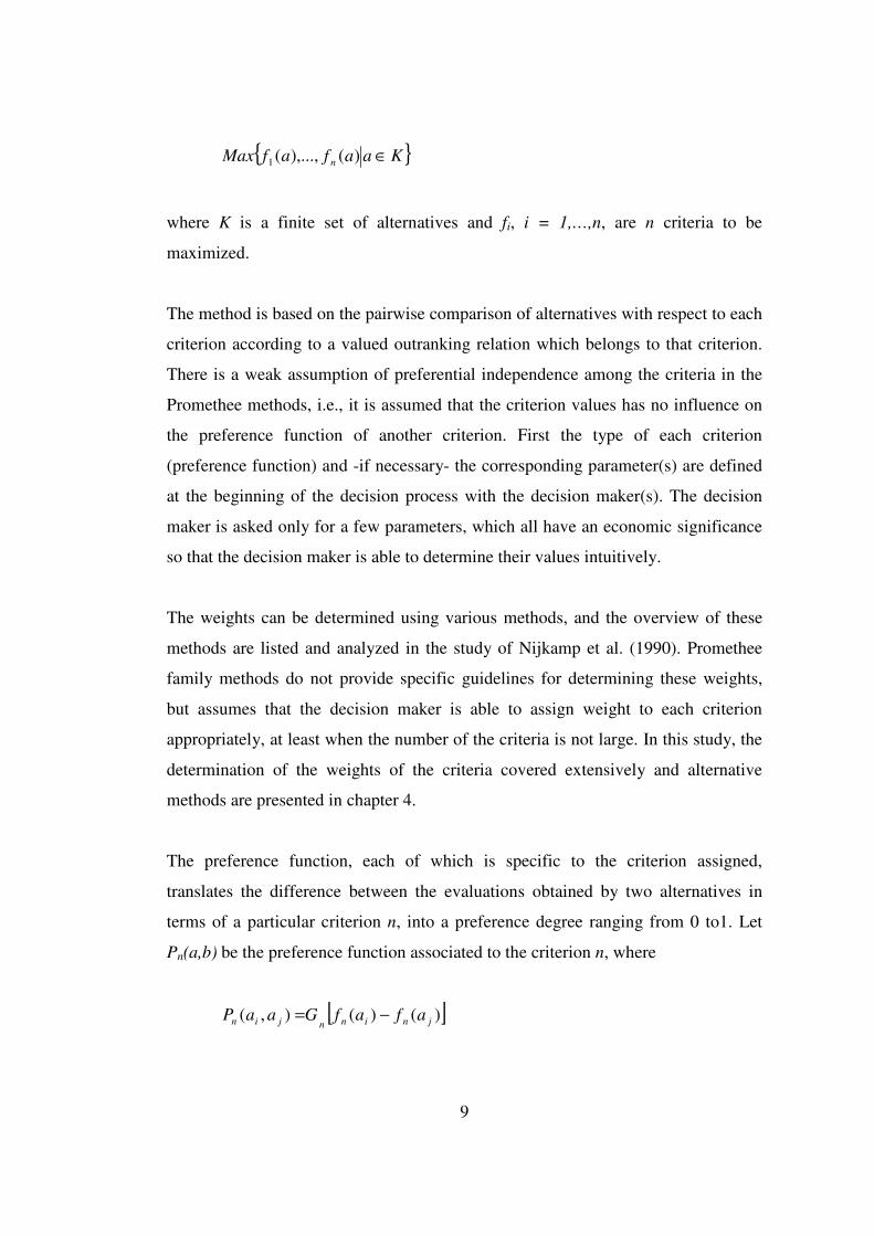
The preference function, each of which is specific to the criterion assigned,

translates the difference between the evaluations obtained by two alternatives in

terms of a particular criterion n, into a preference degree ranging from 0 to1. Let

Pn(a,b) be the preference function associated to the criterion n, where

[ ])()(),( jninnjin afafGaaP −=

10

1),(0 ≤≤ jin aaP

Here Gn is a non-decreasing function of the observed deviation between fn(ai) and

fn(aj). Six basic types of preference functions are proposed for the selection (Brans

et al. 1986).

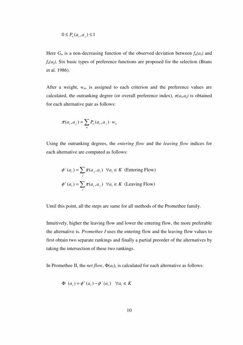
After a weight, wn, is assigned to each criterion and the preference values are

calculated, the outranking degree (or overall preference index), π(ai,aj) is obtained

for each alternative pair as follows:

∑ ⋅=n

njinji waaPaa ),(),(π

Using the outranking degrees, the entering flow and the leaving flow indices for

each alternative are computed as follows:

∑=−

j

iji aaa ),()( πφ Kai ∈∀ (Entering Flow)

∑=+

j

jii aaa ),()( πφ Kai ∈∀ (Leaving Flow)

Until this point, all the steps are same for all methods of the Promethee family.

Intuitively, higher the leaving flow and lower the entering flow, the more preferable

the alternative is. Promethee I uses the entering flow and the leaving flow values to

first obtain two separate rankings and finally a partial preorder of the alternatives by

taking the intersection of these two rankings.

In Promethee II, the net flow, Φ(ai), is calculated for each alternative as follows:

)()()( iii aaa−+ −=Φ φφ Kai ∈∀

11

According to the net flow value of each alternative, a complete preorder on the set

of possible alternatives is proposed to the decision maker.

3.2 ANALYTICAL HIERARCHY PROCESS (AHP)

The analytical hierarchy process (AHP) (Saaty, 1982, 1988, 1995) is one of the best

known and most widely used MCDM approach. In AHP, the top element of the

hierarchy is the overall goal for the decision model. The hierarchy decomposes

from the general to a more specific criterion until a manageable decision criteria is

met. On the other hand it can incorporate both quantitative and qualitative

components in a complex decision making problem.

Overall, AHP is based on three principles, namely construction of the hierarchy,

priority setting and logical consistency.

3.2.1 Construction of the Hierarchy

A decision problem centered around measuring contributions to an overall goal, is

structured and decomposed into its constituent parts (i.e. criteria, sub-criteria

alternatives, etc.), using a hierarchy.

3.2.2 Priority Setting

The relative “priority” given to each element in the hierarchy is determined by

comparing pairwise the contribution of each element at a lower level in terms of the

criteria (or elements) with which a causal relationship exists. The decision maker

uses a pairwise comparison mechanism, the square matrix as shown in Figure 2.1.

12

n

jici

nj

x

xxPx

x

xxxC

M

M

LL

),(

1

1

Figure 3.1 Square matrix

The following statements hold for a pairwise comparison square matrix:

1),( =jic xxP if i = j.

),(1),(

ijcjic xxP

xxP = ∀ (i,j) pairs

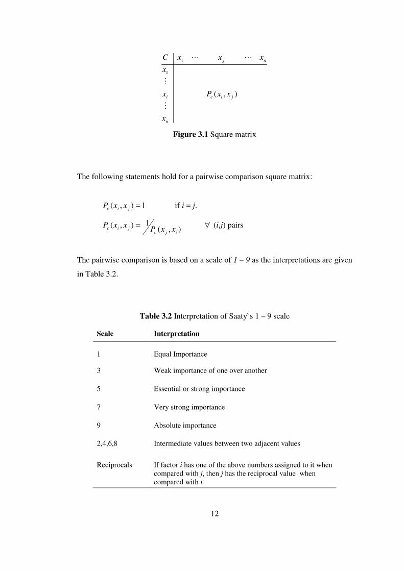
The pairwise comparison is based on a scale of 1 – 9 as the interpretations are given

in Table 3.2.

Table 3.2 Interpretation of Saaty`s 1 – 9 scale

Scale Interpretation

1 Equal Importance

3 Weak importance of one over another

5 Essential or strong importance

7 Very strong importance

9 Absolute importance

2,4,6,8 Intermediate values between two adjacent values

Reciprocals If factor i has one of the above numbers assigned to it when compared with j, then j has the reciprocal value when compared with i.

13

Formally the relative priorities (or weights) of each element with respect to a higher

level element in the hierarchy are given by the right eigenvector (W) corresponding

to the highest eigenvalue (λmax) as follows:

WWA ⋅=⋅ maxλ

The pairwise comparison matrix shown in Figure 3.1 is represented by letter A. Its

standard element is Pc(xi,xj), that is the intensity of the preference (in terms of

contribution to a specific criterion (c) of the row element (xi) over the column

element (xj).

Since the decision maker makes multiple pairwise comparisons among a set of

elements, the problem of “consistency” arises. The consistency check procedure for

the pairwise comparisons is explained in the next section in this chapter.

In case the pairwise comparisons are completely consistent, the matrix A has rank 1

and λmax = n. In that case weights can be obtained by normalizing any of the

columns of A. Else if the consistency check reveals that the comparisons are not

consistent enough, the data entered should be revised and updated by the decision

maker and afterwards the weights could be calculated.

The procedure described above is repeated for all subsystems in the hierarchy. In

order to synthesize various priority vectors, these priorities are weighted with global

priorities of the parent criteria and synthesized. This process starts at the top of the

hierarchy. As a result, the overall relative priority to be given to the lowest elements

is obtained. These overall relative priorities indicate the degree to which the

elements contribute to the top of the hierarchy (goal).

14

3.2.3 Consistency Check

As mentioned in section 3.2.2, in case the pairwise comparisons are completely

consistent, the matrix A has rank 1 and λmax = n. In that case weights can be

obtained by normalizing any of the columns of A. In fact in case of complete

consistency, the following preference relation holds for any subset (ai, aj, ak):

),(),(),( jkckicjic aaPaaPaaP = .,, kji∀

For example, let there be three elements, x, y, z to be compared. If x is preferred to y

and y is preferred to z, then by transitivity property x should be preferred to z. If this

property holds for all the comparisons of the decision maker for some degree, then

the pairwise comparisons are said to be consistent (or consistent enough).

However it is very unlikely for a decision maker to make the pairwise comparisons

through a perfect consistent manner. In case the inconsistency of the pairwise

comparison matrices is limited, slightly the highest eigenvalue (λmax) deviates from

n. This deviation (λmax-n) is used as the measure for inconsistency. This measure is

divided by n-1 to obtain the “consistency index” (CI) as follows:

1

max

−

−=

n

nCI

λ

The final “consistency ratio” (CR), on the basis of which one can conclude whether

the evaluations are sufficiently consistent, is calculated as follows:

*CI

CICR =

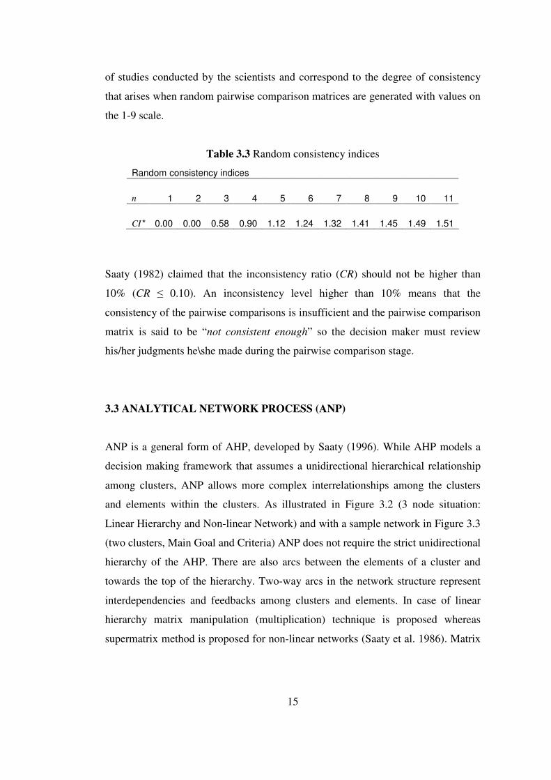
Where CI is the consistency index and CI* is the random consistency index. The

random consistency indices (CI*`s given in Table 3.3) are the experimental results

15

of studies conducted by the scientists and correspond to the degree of consistency

that arises when random pairwise comparison matrices are generated with values on

the 1-9 scale.

Table 3.3 Random consistency indices

Random consistency indices

n 1 2 3 4 5 6 7 8 9 10 11

CI* 0.00 0.00 0.58 0.90 1.12 1.24 1.32 1.41 1.45 1.49 1.51

Saaty (1982) claimed that the inconsistency ratio (CR) should not be higher than

10% (CR ≤ 0.10). An inconsistency level higher than 10% means that the

consistency of the pairwise comparisons is insufficient and the pairwise comparison

matrix is said to be “not consistent enough” so the decision maker must review

his/her judgments he\she made during the pairwise comparison stage.

3.3 ANALYTICAL NETWORK PROCESS (ANP)

ANP is a general form of AHP, developed by Saaty (1996). While AHP models a

decision making framework that assumes a unidirectional hierarchical relationship

among clusters, ANP allows more complex interrelationships among the clusters

and elements within the clusters. As illustrated in Figure 3.2 (3 node situation:

Linear Hierarchy and Non-linear Network) and with a sample network in Figure 3.3

(two clusters, Main Goal and Criteria) ANP does not require the strict unidirectional

hierarchy of the AHP. There are also arcs between the elements of a cluster and

towards the top of the hierarchy. Two-way arcs in the network structure represent

interdependencies and feedbacks among clusters and elements. In case of linear

hierarchy matrix manipulation (multiplication) technique is proposed whereas

supermatrix method is proposed for non-linear networks (Saaty et al. 1986). Matrix

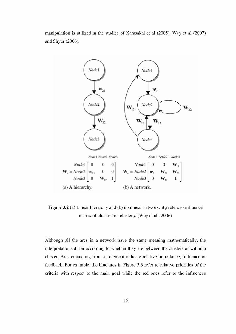
16

manipulation is utilized in the studies of Karasakal et al (2005), Wey et al (2007)

and Shyur (2006).

Figure 3.2 (a) Linear hierarchy and (b) nonlinear network. Wij refers to influence

matrix of cluster i on cluster j. (Wey et al., 2006)

Although all the arcs in a network have the same meaning mathematically, the

interpretations differ according to whether they are between the clusters or within a

cluster. Arcs emanating from an element indicate relative importance, influence or

feedback. For example, the blue arcs in Figure 3.3 refer to relative priorities of the

criteria with respect to the main goal while the red ones refer to the influences

17

Main Goal

C1 C2

C3

C4

Cluster 1

Element: Main Goal

Cluster 2

Elements: Criteria

(C1, C2, C3 and C4)

Inter-cluster influence

Within cluster influence - interdependency

Feedbacks

between the criteria and the black ones are the feedbacks from criteria to main goal.

The corresponding values of the arcs are measured on a ratio scale similar to AHP.

ANP approach is capable of handling interdependency among elements by

obtaining the composite weights through the development of a supermatrix. The

supermatrix is the combination of individual square matrices that correspond to

each cluster. They represent the network within each cluster. All in all, the

supermatrix is a single matrix showing all the elements in all clusters.

Figure 3.3 Illustration of a sample ANP network

18

Saaty explains the supermatrix concept parallel to the Markov Chain Processes. By

incorporating interdependencies (i.e. addition of the feedback arcs in the model), the

supermatrix is created. Feedback arcs are important because there should exist

complete loops for supermatrix application. In other words, from the Markov

Chains point of view, all the elements (nodes) should be recurrent instead of being

transient so that the effects of the influences on the final results do not vanish for

some elements (nodes) during the application.

Assume that there is a system of N clusters where the elements in each cluster have

impact on or are influenced by some or all of the elements of that cluster or of other

clusters with respect to a property governing the interactions of the entire system.

Assume that cluster h, denoted by Ch, h=1,…,N, has n elements denoted by eh1,

eh2,…,ehn. The structure of the corresponding supermatrix is illustrated in Figure 3.4.

During building up the supermatrix, it is extremely important to be consistent about

the question asked to the decision maker. Saaty (1999) proposes two types of

questions formulated in terms of dominance or influence. Given a parent element,

which of two elements being compared with respect to it has greater influence (is

more dominant) on that parent element? Or, which is influenced more with respect

to that parent element?

For example, in comparing A to B (elements in a cluster) with respect to a criterion,

the question asked is whether the criterion influences A or B more. Then if for the

next comparison involving A and C the question asked is whether A or C influences

the criterion more, this would be a change in perspective that would undermine the

whole process. One must keep in mind whether the influence is flowing from the

parent element to the elements being compared, or the other way around.

Considering this, it is crucial to stick to the perspective during the pairwise

comparisons

19

NNNN

Nn

N

N

N

N

n

N

n

NnNNnn

N

WWW

e

e

e

C

WWW

e

e

e

C

WWW

e

e

e

C

eeeeeeeee

CCC

N

N

L

M

MOMMMM

LM

LM

LLLL

L

212

1

22221

2

22

21

2

11211

1

12

11

1

212222111211

21

2

1

21

Figure 3.4 The supermatrix

Saaty suggests one of the following two questions throughout a process:

1. Given a parent element and comparing elements A and B under it, which

element has greater influence on the parent element?

(The direction of the arrow is to the parent element)

2. Given a parent element and comparing elements A and B, which element is

influenced more by the parent element?

(The direction of the arrow is from the parent element)

20

To be consisted throughout this study, the first question is posed during the pairwise

comparisons. That is, the eigenvector in the column of an element (either the main

goal or any of the criteria) in the supermatrix indicates the relative influences of the

row elements on the column element. In other words, the numbers in a column are

the relative priorities of the elements with respect to the element corresponding to

that column.

After the pairwise comparisons, each eigenvector is obtained and introduced in the

appropriate position as a column vector as shown in Figure 3.4. While building up

the supermatrix, the eigenvectors in the individual matrices are adjusted by

normalization with respect to the relative weights of the clusters they belong. When

this is done, the supermatrix becomes column stochastic and from this point on it is

called “weighted supermatrix”. This should be performed before any operation on

the supermatrix in order to derive meaningful limiting priorities. From the network

perspective, this operation makes the sums of the arrows emanating from an

element equal to unity, which is essential from the Markov Chains point of view

before any limiting operations on the supermatrix. In general the supermatrix is

rarely stochastic because, in each column, it consists of several eigenvectors each

sums up to one, and hence the entire column of the matrix may sum up to an integer

greater than one. Normalization would be meaningless and such weighting does not

call for normalization.

When the matrix is column stochastic, the limiting priorities depend on its

reducibility and periodicity properties (Kulkarni 1999). (Analogy: Here the term

“limiting priorities” could be perceived as the “limiting probabilities” concept of the

Discrete Time Markov Chains (DTMC). Mathematically, both terms refer to exactly

the same value). Because of the existence of the feedback arcs, the elements of the

supermatrix become recurrent, that is the supermatrix is irreducible form the DTMC

point of view.

21

However, for limiting operations, it is important whether the supermatrix is periodic

or aperiodic. According to the definition given below within the context of DTMC

the supermatrix has to be aperiodic before being raised up to powers. (Here again

there is analogy between the supermatrix and the “one step transition matrix” of

DTMC):

Definition (Periodicity), (Kulkarni, 1999). Let {Xn, n > 0} be an irreducible DTMC

on state space S = {1,2,…,N}, and let d be largest integer such that

⇒>== 0)( 0 iXiXP n n is an integer multiple d,

for all Si ∈ . The DTMC is said to be periodic with period d if d > 1 and aperiodic

if d = 1.

A DTMC with period d can return to its starting state only at times d, 2d, 3d,…. In

particular if 0)( 01 >== iXiXP for any Si ∈ for the irreducible DTMC, than d

must be 1, and the DTMC must be aperiodic. The interpretation of this fact from the

ANP (Supermatrix) point of view is as follows: If at least there is one element that

has a self-influence (in the network the arrow emanates from and ends at the same

element), then the supermatrix is said to be aperiodic. Since, in the methodology

developed, all the criteria have self-influences, there is no risk for the weighted

supermatrix to be periodic.

The weighted supermatrix is raised to a sufficiently large power until the priorities

converges to stable values. An irreducible and aperiodic weighted supermatrix

yields a limiting matrix with all the columns equal to each other. After the limiting

operation, the values corresponding to the elements of the cluster under

consideration are normalized among themselves to obtain the relative weights.

22

3.4. PROSPECT THEORY

Decision maker(s)’ choice behavior is an important issue for the modeling of

decision making problems. For decades, the classical expected utility theory

developed by Keeney and Raiffa (1976) had been accepted as the dominant

paradigm. However, there has been a general agreement that the theory does not

represent the actual decision behavior of the decision maker(s). Many empirical

studies proved that decision maker(s) systematically violate this theory’s basic

tenets. Kahneman and Tversky (1979) came up with a new theory called the

Prospect Theory, which explains the major violations of utility theory and the

intransitive behavior represented by the decision maker.

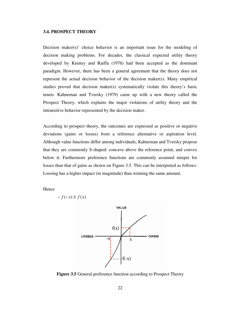
According to prospect theory, the outcomes are expressed as positive or negative

deviations (gains or losses) from a reference alternative or aspiration level.

Although value functions differ among individuals, Kahneman and Tversky propose

that they are commonly S-shaped: concave above the reference point, and convex

below it. Furthermore preference functions are commonly assumed steeper for

losses than that of gains as shown on Figure 3.5. This can be interpreted as follows:

Loosing has a higher impact (in magnitude) than winning the same amount.

Hence

)()( xfxf ≥−−

Figure 3.5 General preference function according to Prospect Theory

f(-x)

f(x)

x -x

23

Prospect theory was originally developed for single criterion problems with

uncertainty, but the ideas have been extended to multiple criteria decision making

problems as well by Korhonen, et al. (1990). Salminen (1994), Karasakal et al.

(2005) and Karasakal & Özerol (2006) also incorporated the Prospect Theory into

MCDM. Apart from these studies, application of prospect theory in MCDM is not

studied much and there are very limited resources in the literature.

24

CHAPTER 4

THE PROPOSED METHODOLOGY

The methodology proposed in this study is a combination of different

methodologies that are individually very common, easy to understand and popular

among the researchers in the field of multi-criteria decision making problems. Each

methodology has a specific advantage with respect to different perspectives, and

they are applicable for a problem only if some specific criteria corresponding to the

methodology are met. Bringing up the useful properties of some methods and

combining them to develop a hybrid methodology has been accepted as an

important progress for some years in the field of MCDM and studied by many

researchers. For example, Lee et al. (2001) proposed an integrated approach for

solving interdependent multi-criteria IS project selection problems using Delphi,

ANP and 0-1 GP. On the other hand, in the study of Macharis et al. (2004), AHP

and PROMETHEE family methods are analyzed and discussed thoroughly and they

state that operational synergies could be achieved by integrating Promethee and a

number of elements associated with AHP. They proposed that AHP could be used

during the weight determination stage of PROMETHEE method, in which no

particular weighing approach was suggested. Similarly, Wang et al. (2006)

combined AHP and PROMETHEE to form a hybrid method to rank alternatives.

They used AHP for the determination of the weights of the criteria and to

understand the structure of the problem, on the other hand PROMETHEE for the

final ranking.

The developed methodology is explained in detail in this chapter. In the first part,

alternative procedures proposed for the determination of the weight of the criteria

are described. And in the second part Promethee II application is explained where

25

new preference functions reflecting decision behavior of the decision maker are

introduced.

4.1 DETERMINATION OF THE CRITERION WEIGHTS

The most crucial part of the multi-criteria decision making problem is to specify the

weights of the criteria, which in essence, is the most determining stage for the final

solution. Therefore, an intense care is spent throughout the study. Three alternative

techniques, which are proposed to the decision maker, are presented in this part for

weight determination.

4.1.1 Technique 1: AHP (Independent criteria)

In most cases to simplify the procedure in MCDM problems, the criteria are

assumed to be independent of each other, that is, there are no interrelationships

between the criteria. In other words, the existence or non-existence of a criterion

has no effect on others. Simply AHP is utilized in such cases for the determination

of the weights of the criteria. The question posed to the decision maker during the

pairwise comparisons is as follows:

“Which criterion is more important with respect to the main goal and how

much?”

In this technique the decision maker makes ½*(n-1)*(n-2) pairwise comparisons

(should be consistent enough), where n is the total number of criteria, and the

eigenvector corresponding to the highest eigenvalue yields the weights for criteria

Wo.

26

4.1.2 Technique 2: Matrix Multiplication Method

Matrix multiplication is composed of three phases. In the first phase just like in

technique 1, the original weights, Wo of the criteria are calculated using AHP

ignoring the interdependencies among them.

In the second phase the relative influences on each other is obtained again using

AHP. Considering each criterion, a pairwise comparison is made among all criteria

in terms of the magnitude of the impact inflicted on the criterion under

consideration. The comparisons are made according to the Saaty’s 1 - 9 scale (Table

3.2). During the pairwise comparisons, the decision maker is supposed to answer

the following question:

“Given a reference criterion, which criterion influences the criterion under

consideration more and how much?”

Again here the consistency plays an important role, that is, the pairwise

comparisons of the decision maker must be consistent enough among themselves.

Suppose there are n criteria and the comparison matrix is formed as shown in Figure

4.1.

1

1

1

1

111

1

LL

MMMM

LL

MMMM

LL

LL

inkinn

ijnijkijj

niki

nki

xxC

xxxC

xxC

CCCC

Figure 4.1 The criteria comparison matrix w.r.t. criteria i

In the comparison matrix xijk refers to the factor that how many times more the

criterion j influences the parent (reference) criterion i than the criterion k.

27

After the comparison matrix is formed, the eigenvector corresponding to the highest

eigenvalue is calculated, yielding the relative influences of the criteria on the

criterion i:

],,[ 1 nijii

T

i xxxE LL=

At this point, one must notice that these numbers are not the weights of the criteria

with respect to the main goal; instead they can be interpreted as the relative

influences on the criterion under consideration.

Similarly all the eigenvectors for each criterion are obtained and brought together to

form the impact matrix, E, as shown in Figure 4.2. In the impact matrix, xji refers to

the relative influence of criterion j on criterion i.

nnninn

jnjijj

ni

ni

xxxC

xxxC

xxxC

CCC

E

LL

MMMM

LL

MMMM

LL

LL

1

1

11111

1

=

Figure 4.2 The impact matrix

Lastly, the final weights W, of the criteria are obtained as follows:

oWEW ×=

Where

E : Impact matrix

Wo : Weights obtained assuming there is no interdependency

W : Final weights of the criteria

28

4.1.3 Technique 3: ANP - The Supermatrix Method

This technique is proposed if there exist interdependencies among criteria. It utilizes

the supermatrix phenomena introduced by Saaty (1996) as the tool for the ANP

concept. Since ANP can handle the interrelationships among the clusters and the

elements, it can be used as the weight determination tool where there are

interdependencies.

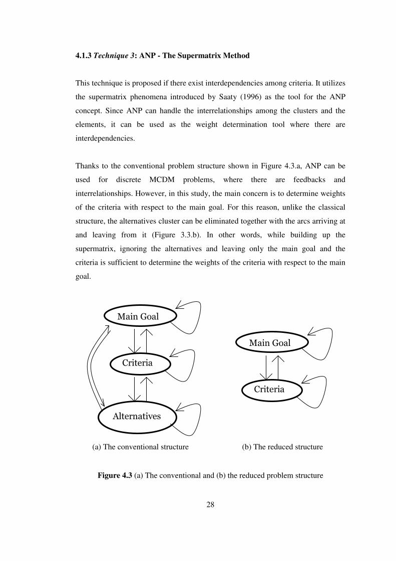
Thanks to the conventional problem structure shown in Figure 4.3.a, ANP can be

used for discrete MCDM problems, where there are feedbacks and

interrelationships. However, in this study, the main concern is to determine weights

of the criteria with respect to the main goal. For this reason, unlike the classical

structure, the alternatives cluster can be eliminated together with the arcs arriving at

and leaving from it (Figure 3.3.b). In other words, while building up the

supermatrix, ignoring the alternatives and leaving only the main goal and the

criteria is sufficient to determine the weights of the criteria with respect to the main

goal.

Figure 4.3 (a) The conventional and (b) the reduced problem structure

Main Goal

Criteria

Main Goal

Criteria

AlternativesIVESr

(a) The conventional structure (b) The reduced structure

29

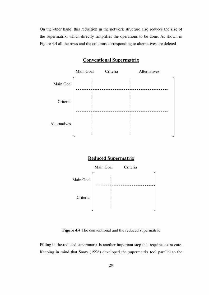
On the other hand, this reduction in the network structure also reduces the size of

the supermatrix, which directly simplifies the operations to be done. As shown in

Figure 4.4 all the rows and the columns corresponding to alternatives are deleted

Figure 4.4 The conventional and the reduced supermatrix

Filling in the reduced supermatrix is another important step that requires extra care.

Keeping in mind that Saaty (1996) developed the supermatrix tool parallel to the

Reduced Supermatrix

Main Goal

Criteria

Main Goal Criteria

Conventional Supermatrix

Main Goal

Criteria

Alternatives

Main Goal Criteria Alternatives

30

“Markov Chains” concept, it is useful to construct the analogy. That is, considering

every criteria and the main goal as the nodes or states, which are the elements of the

set of possible outcomes, introduces meaning and significance to the technique

applied

At this point, there is an important question that the decision maker has to answer:

“By how much amount do you want the interdependencies among the

criteria to take effect on the final weights of the criteria?”

Answering this question, the decision maker decides on the weights of the two

clusters. They are the Main Goal cluster, which has only a single element the main

goal, and the criteria cluster whose elements are the criteria. The weights are

specified in a way that the sum equals to 1, that is

1=+ cm WW

where

Wm: weight of the main goal cluster (influence of the original weights)

Wc: weight of the criteria cluster (influence of the interdependency)

And the notation for the ANP application is ANP(w1, w2), where

mWw =1 and cWw =2

For example, let’s say in case 1, the decision maker sets Wc=0.1, Wm automatically

becomes 0.9, which means that original weights have 9 times more impact on the

final weights than the interdependencies. And in case 2 it is vice versa. According

to these numbers, in case 1, the technique will yield closer solution to the original

weights than in case 2.

31

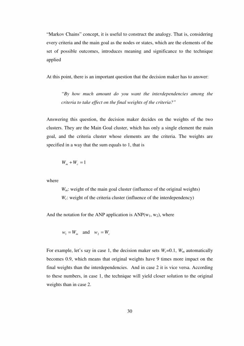
After determining the weights of the two clusters, the supermatrix can be filled.

First the original weights of the criteria with respect to main goal are determined as

if there is no interdependency among them just like in technique 1 and the numbers

obtained are inserted into the first column to the corresponding rows, in the region

II as indicated in Figure 4.5. Second the impact matrix, E, whose columns sum to

unity, is obtained as described in technique 2. Before inserting the impact matrix

into region III, it is updated by multiplying with Wc, weight of the criteria cluster,

hence column sums of region III equals Wc.

IIIIICriteria

IVIMainGoal

CriteriaMainGoal

S =

Region I: Influence of main goal on main goal

Region II: Relative influences of criteria on main goal

Region III: Relative influences of criteria on criteria

Region IV: Influence of main goal on criteria

Figure 4.5 Regions of the reduced supermatrix and interpretations

Finally every element of the region IV is set to Wm, indicating the objective position

of the main goal with respect to the interdependencies within the criteria cluster.

The single node in region I is set to zero, because it has no effect in the final results

even when set to a positive number, but only reduces the convergence speed during

the limiting operations.

All in all, one must spent extra care while computing the eigenvectors in the regions

II and III. For convenience, the question asked during the pairwise comparisons for

these regions are given below (one must note that no question is asked for region I

32

since its value is entered zero and the value for region IV is manipulated according

the cluster weights):

“With respect to the main goal, which criterion has more influence and how

much?” (Region II)

“Given the reference criterion, which criterion has more influence on the

criterion under consideration and how much?” (Region III).

Finally the supermatrix is constructed as shown below. Before proceeding with the

operations on the supermatrix, one must note that it is important to check that the

supermatrix is column stochastic, i.e. all the column sums up to unity.

EWWCriteria

WMainGoal

CriteriaMainGoal

S

co

m

⋅

= 0

nncncnconn

nccco

nccco

mmm

n

xWxWxWWC

xWxWxWWC

xWxWxWWC

WWWMainGoal

CCCMainGoal

S

⋅⋅⋅

⋅⋅⋅

⋅⋅⋅=

L

MOMMMM

L

L

L

L

21

2222122

1121111

21

0

where

Exij ∈ nji ,...,2,1:,

and

1=∑N

i

ijx ∀ nj ,...,2,1:

33

At this point the analogy with the Markov Chains (MC) concept could be set as

follows: All the elements within the clusters (i.e. the main goal and the criteria)

could be perceived as states of a Discrete Time Markov Chain (DTMC) and the set

of possible outcomes (states) conforms an irreducible closed set in which all the

states are recurrent. From DTMC point of view, the supermatrix S obtained is the

one-step transition matrix. Intuitively the limiting probabilities to be obtained will

refer to the priorities of the elements. Since the one-step transition matrix

(supermatrix, S) is irreducible and aperiodic as explained in section 3.3, the

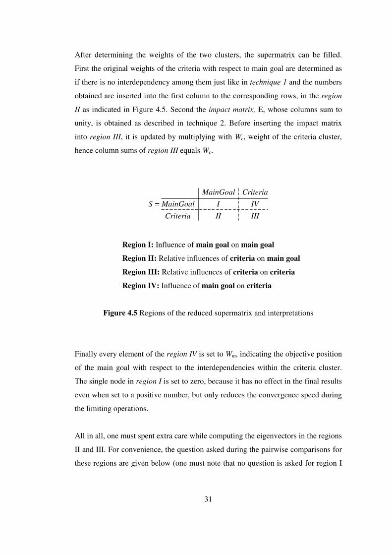
Limiting Probabilities, π could be obtained as follows:

),(lim jiSn

n ∞→=π

Not necessarily it is required to raise the supermatrix to a high degree power,

instead in most cases it is sufficient to raise it to the power in the order of 100`s,

because the system rapidly converges, and an ordinary CPU performs this operation

within seconds for a 10x10 supermatrix (9 criteria and the main goal for example).

During the operation, one must spend special care that the supermatrix is column

stochastic, otherwise the matrix does not converge.

The columns of the obtained limiting matrix are exactly same and it sums up to

unity. The numbers corresponding to the criteria in region III must be re-normalized

since the number corresponding to the main goal element does not have any

significant role. The re-normalized numbers are the weights of the criteria with

respect to the main goal in the case of existence of interrelationships among criteria.

All in all, the criteria weights are computed considering that all the criteria are at the

same level (single cluster). However, when the number of the criteria is large,

constructing the impact matrix is not an easy task in case of existence of

interdependency. For such situations the criteria could be rearranged such that sub-

clusters are formed. Also in some problem, there must be some sub-clusters due to

the nature of the problem. For such cases, instead of handling all the criteria at a

34

single step simultaneously, simple operations could be performed on the sub-

clusters using the matrix manipulation technique (Saaty et al. 1986) and the

composite weights of the criteria could be obtained.

4.2 PROMETHEE II APPLICATION

After the determination of the weights of the criteria, alternatives could be ranked

with Promethee II method. Like the weight determination stage, this part also

requires interaction with the decision maker, in order to understand his/her

perception of each criterion one by one.

At this stage, through an interactive procedure, the proposed methodology tries to

grab three important aspects of the problem, which are crucial all the way towards

the solution:

1. For a specific criterion, does the decision maker have a preference function

that is parallel to prospect theory?

2. For a specific criterion, which preference function among the presented

types, best suit and represent nature of that criterion?

3. What are the values of the parameters which are specific for the type of the

preference function determined?

In the beginning, during the construction of the problem, while introducing the

criteria, the decision maker is asked the following question for each criterion:

“Considering the criterion under consideration, minimum how many unit(s)

of gain can satisfy you upon one unit of loss?”

35

From the utility theory point of view, the answer should be always “one”, which

makes sense mathematically. From the prospect theory point of view, this is not

always the case; generally “more than one” unit of gain is necessary for satisfaction.

For this reason, according to the answer given to the question above, two groups of

preference functions are proposed to the decision maker.

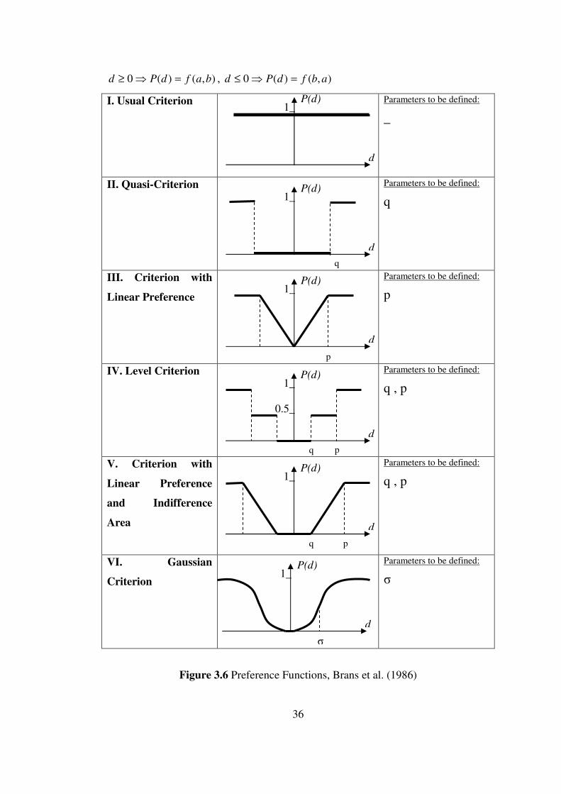
I. If the answer is “one”, the six basic types of preference functions

defined in the study of Brans et al. (1986) (I, II, .., VI) are

proposed. These functions and the parameters required for each

function are summarized in Figure 4.6. What is significant here is

that these functions are symmetrical with respect to the vertical

axis.

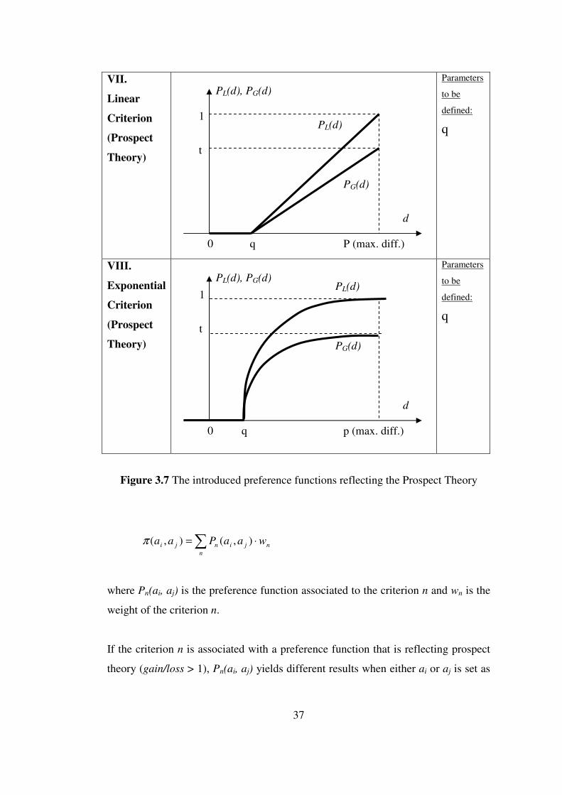
II. If the answer is “more than one”, two new preference functions,

VII and VIII, in accordance with prospect theory are proposed

because this answer is perceived as the indication of prospect

theory in the choice behavior of the decision maker for the

criterion under consideration. These two preference functions are

illustrated in Figure 4.7 and explained in detail in section 4.3. One

must note that symmetrical property of the previous set of

functions does not exist in this new set of functions.

After decision maker specifies all the preference functions and corresponding

parameters for each criterion, the Promethee II method can be applied for the

complete ranking.

In the methodology developed, the crucial part of the Promethee II application is the

incorporation of the prospect theory. As explained in the previous chapter, the

overall preference index of an alternative pair is calculated as

36

),()(0 bafdPd =⇒≥ , ),()(0 abfdPd =⇒≤

I. Usual Criterion Parameters to be defined:

_

II. Quasi-Criterion Parameters to be defined:

q

III. Criterion with

Linear Preference

Parameters to be defined:

p

IV. Level Criterion Parameters to be defined:

q , p

V. Criterion with

Linear Preference

and Indifference

Area

Parameters to be defined:

q , p

VI. Gaussian

Criterion

Parameters to be defined:

σ

Figure 3.6 Preference Functions, Brans et al. (1986)

d

P(d) 1_

d

P(d) 1_

q

p

d

P(d) 1_

d

P(d) 1_

p q

d

P(d) 1_

p q

d

P(d) 1_

σ

0.5_

37

VII.

Linear

Criterion

(Prospect

Theory)

Parameters

to be

defined:

q

VIII.

Exponential

Criterion

(Prospect

Theory)

Parameters

to be

defined:

q

Figure 3.7 The introduced preference functions reflecting the Prospect Theory

∑ ⋅=n

njinji waaPaa ),(),(π

where Pn(ai, aj) is the preference function associated to the criterion n and wn is the

weight of the criterion n.

If the criterion n is associated with a preference function that is reflecting prospect

theory (gain/loss > 1), Pn(ai, aj) yields different results when either ai or aj is set as

p (max. diff.)

d

PL(d), PG(d)

t

1 PL(d)

PG(d)

0

q P (max. diff.)

d

PL(d), PG(d)

t

1 PL(d)

PG(d)

0

q

38

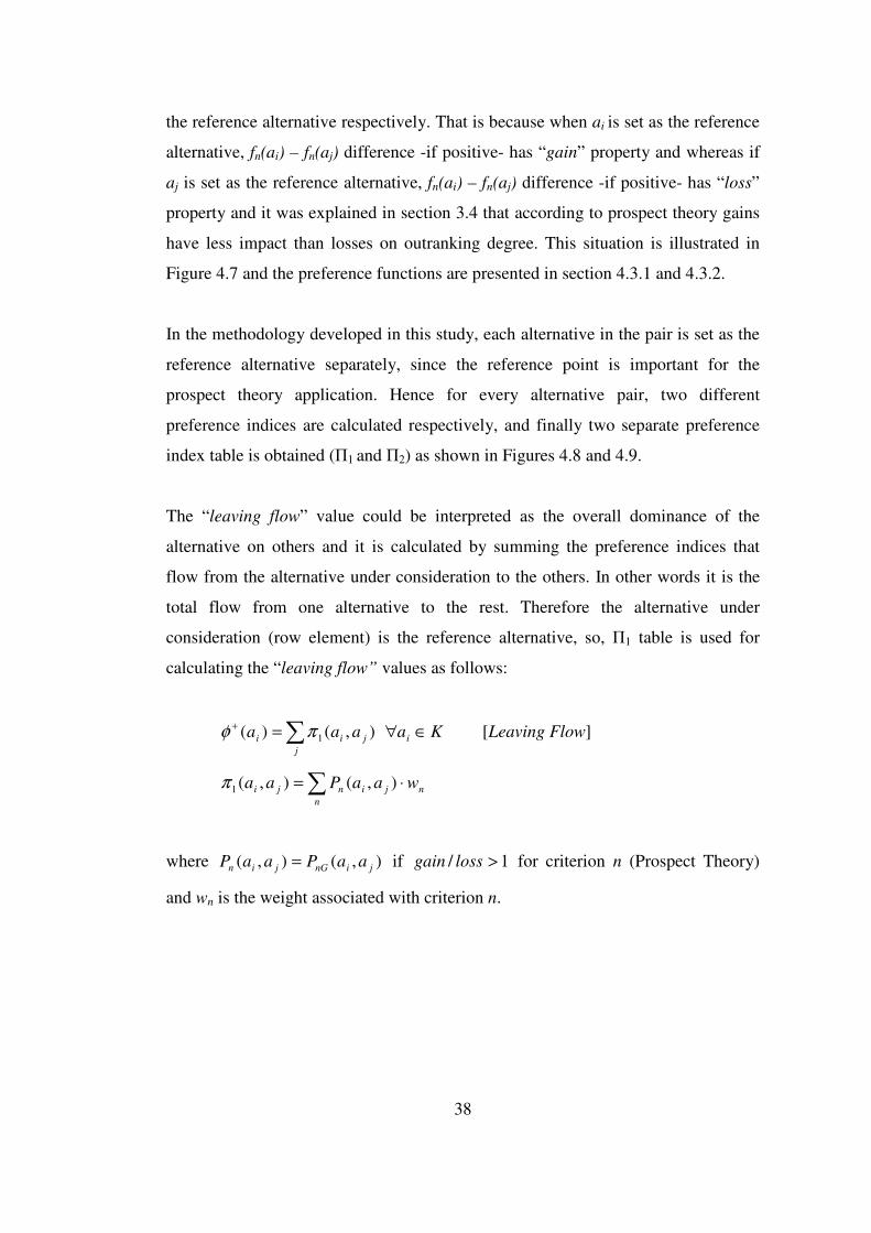
the reference alternative respectively. That is because when ai is set as the reference

alternative, fn(ai) – fn(aj) difference -if positive- has “gain” property and whereas if

aj is set as the reference alternative, fn(ai) – fn(aj) difference -if positive- has “loss”

property and it was explained in section 3.4 that according to prospect theory gains

have less impact than losses on outranking degree. This situation is illustrated in

Figure 4.7 and the preference functions are presented in section 4.3.1 and 4.3.2.

In the methodology developed in this study, each alternative in the pair is set as the

reference alternative separately, since the reference point is important for the

prospect theory application. Hence for every alternative pair, two different

preference indices are calculated respectively, and finally two separate preference

index table is obtained (Π1 and Π2) as shown in Figures 4.8 and 4.9.

The “leaving flow” value could be interpreted as the overall dominance of the

alternative on others and it is calculated by summing the preference indices that

flow from the alternative under consideration to the others. In other words it is the

total flow from one alternative to the rest. Therefore the alternative under

consideration (row element) is the reference alternative, so, Π1 table is used for

calculating the “leaving flow” values as follows:

∑=+

j

jii aaa ),()( 1πφ Kai ∈∀ [Leaving Flow]

∑ ⋅=n

njinji waaPaa ),(),(1π

where ),(),( jinGjin aaPaaP = if 1/ >lossgain for criterion n (Prospect Theory)

and wn is the weight associated with criterion n.

39

∑

∑

∑

∑

+Π

j

jkkkjkkkk

j

jikijiiii

j

jkj

j

jkj

ikj

aaaaaaaaaaa

aaaaaaaaaaa

aaaaaaaaaaa

aaaaaaaaaaa

aaaaa

),(),(),(),(),(

),(),(),(),(),(

),(),(),(),(),(

),(),(),(),(),(

)(

1112111

1112111

2121212211212

1111112111111

211

πππππ

πππππ

πππππ

πππππ

φ

LL

MMOMLMMM

LL

MMMMOMMM

LL

LL

LL

Figure 4.8 Preference indices table (Π1) and calculation of leaving flows, )( ia+φ

(first elements of the alternative pairs are the reference alternatives)

∑∑∑∑−

Π

i

ki

i

ji

i

i

i

ij

kkjkkkk

kijiiii

kj

kj

kj

aaaaaaaaa

aaaaaaaaa

aaaaaaaaa

aaaaaaaaa

aaaaaaaaa

aaaa

),(),(),(),()(

),(),(),(),(

),(),(),(),(

),(),(),(),(

),(),(),(),(

222212

222212

222212

22222221222

12122121121

212

ππππφ

ππππ

ππππ

ππππ

ππππ

LL

LL

MOMMMMM

LL

MMMOMMM

LL

LL

LL

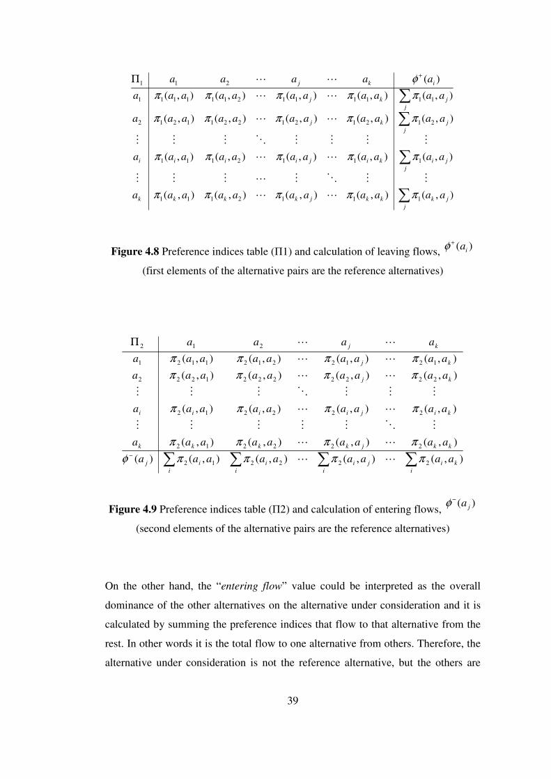
Figure 4.9 Preference indices table (Π2) and calculation of entering flows, )( ja

−φ

(second elements of the alternative pairs are the reference alternatives)

On the other hand, the “entering flow” value could be interpreted as the overall

dominance of the other alternatives on the alternative under consideration and it is

calculated by summing the preference indices that flow to that alternative from the

rest. In other words it is the total flow to one alternative from others. Therefore, the

alternative under consideration is not the reference alternative, but the others are

40

(column elements), so Π2 table is used for calculating the “entering flow” values as

follows:

∑=−

i

jij aaa ),()( 2πφ Ka j ∈∀ (Entering Flow)

∑ ⋅=n

njinji waaPaa ),(),(2π

where ),(),( jinLjin aaPaaP = if 1/ >lossgain for criterion n (Prospect Theory)

and wn is the weight associated with criterion n.

All in all, two different preference indices tables are obtained for the calculation of

flow values. In the first one (Π1), the first elements in the alternative pairs (row

elements) are set as the reference alternatives, i.e. the criteria value differences have

“gain” property. Whereas in the second table (Π2), the second elements in the

alternative pairs (the column elements) are set as the reference alternatives, i.e. the

criteria value differences have “loss” property. The “net flow” values are calculated

using the “leaving flow” and the “entering flow” values and the final ranking of the

alternatives are obtained.

If in the beginning of the problem, all the answers to the “gain/loss” ratio question

is given as “1” by the decision maker, the two preference indices tables become

equal (Π1 = Π2), which makes sense and the problem returns to an ordinary

Promethee II application.

4.3 THE INTRODUCED PREFERENCE FUNCTIONS

Two new preference functions, which are suitable for the Prospect Theory

applications are introduced in this study and proposed to the decision maker in the

methodology. The first one is a variation of the preference function V, criterion

with linear preference and indifference area, proposed by Brans et al. (1986). The

41

second one is a variation of the preference function proposed by Karasakal et al.

(2005) and it is based on exponential function. Both are explained in detail below.

The decision maker must choose either one of these two in case his/her perception

of the criteria under consideration best suits to the prospect theory. The most

significant difference of the two is that one is linear; the other is concave, whereas

both have an indifference area, which are specified by defining the corresponding

indifference threshold value. On the other hand, if the contribution of small

differences of the criterion value beyond the indifference area is significant, then it

would be more appropriate for the decision maker to choose the preference function

VIII (exponential function) because this function has a steeper slope just after the

indifference area.

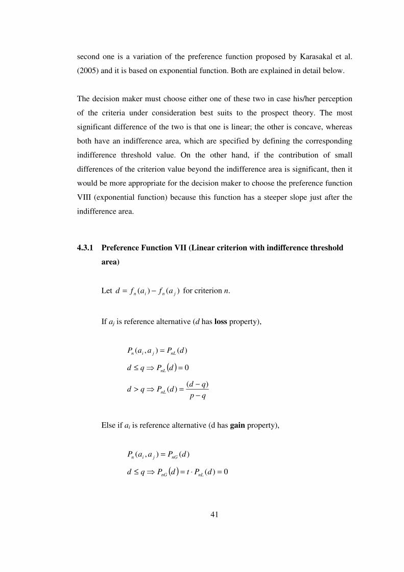
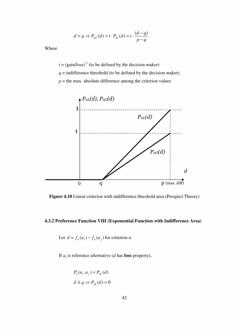
4.3.1 Preference Function VII (Linear criterion with indifference threshold

area)

Let )()( jnin afafd −= for criterion n.

If aj is reference alternative (d has loss property),

)(),( dPaaP nLjin =

( ) 0=⇒≤ dPqd nL

qp

qddPqd nL

−

−=⇒>

)()(

Else if ai is reference alternative (d has gain property),

)(),( dPaaP nGjin =

( ) 0)( =⋅=⇒≤ dPtdPqd nLnG

42

qp

qdtdPtdPqd nLnG

−

−⋅=⋅=⇒>

)()()(

Where

t = (gain/loss)-1 (to be defined by the decision maker)

q = indifference threshold (to be defined by the decision maker)

p = the max. absolute difference among the criterion values

Figure 4.10 Linear criterion with indifference threshold area (Prospect Theory)

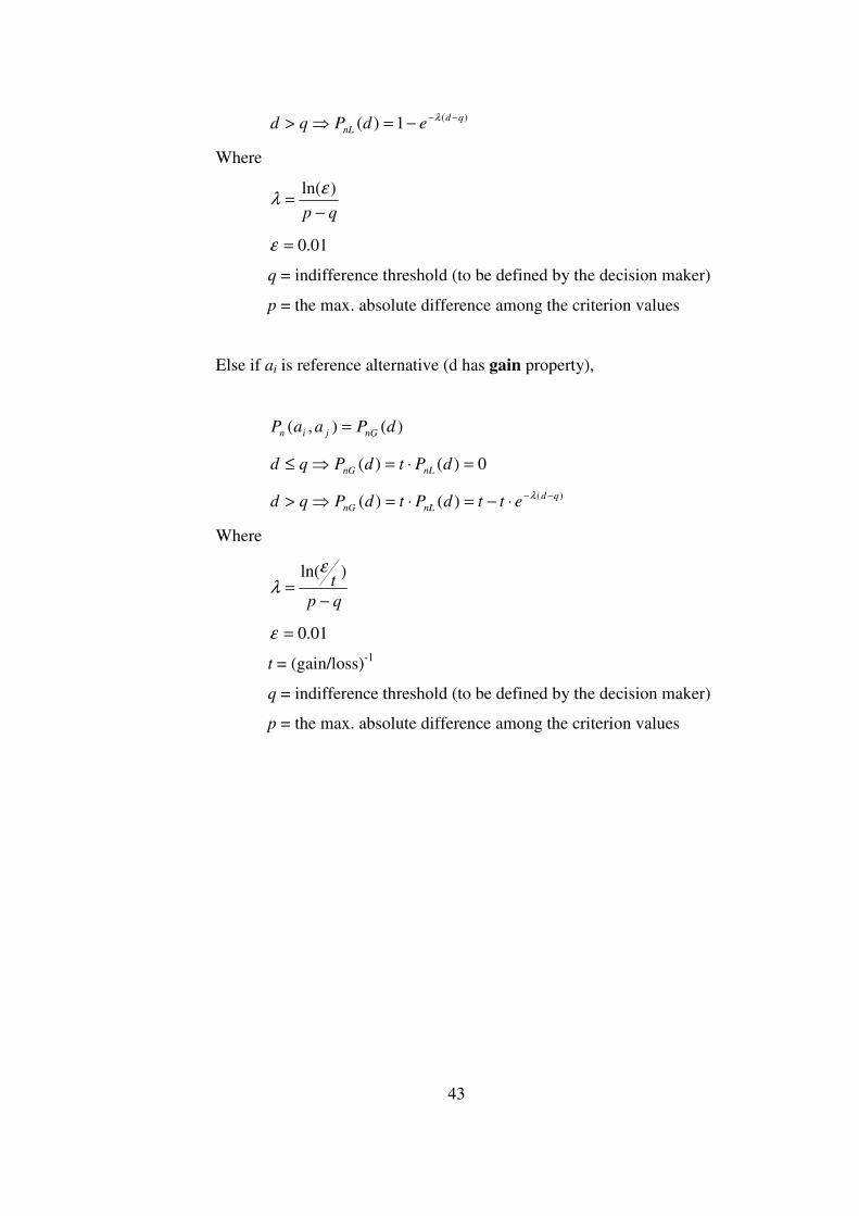
4.3.2 Preference Function VIII (Exponential Function with Indifference Area)

Let )()( jnin afafd −= for criterion n.

If aj is reference alternative (d has loss property),

)(),( dPaaP nLjin =

0)( =⇒≤ dPqd nL

0 p (max. diff)

d

PnL(d), PnG(d)

1

t

PnL(d)

PnG(d)

q

43

)(1)( qd

nL edPqd−−−=⇒> λ

Where

qp −=

)ln(ελ

01.0=ε

q = indifference threshold (to be defined by the decision maker)

p = the max. absolute difference among the criterion values

Else if ai is reference alternative (d has gain property),

)(),( dPaaP nGjin =

0)()( =⋅=⇒≤ dPtdPqd nLnG

)()()( qd

nLnG ettdPtdPqd−−⋅−=⋅=⇒> λ

Where

qp

t

−=

)ln(ελ

01.0=ε

t = (gain/loss)-1

q = indifference threshold (to be defined by the decision maker)

p = the max. absolute difference among the criterion values

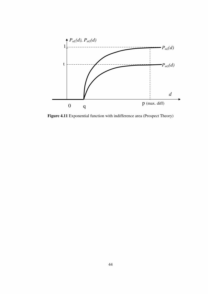
44

Figure 4.11 Exponential function with indifference area (Prospect Theory)

p (max. diff)

d

PnL(d), PnG(d)

1_

t

PnL(d)

PnG(d)

0 q

45

CHAPTER 5

THE SOFTWARE

In this chapter, the developed software is introduced thoroughly together with

demonstrations of the windows of the user interface. Also the algorithm is

summarized with the flowchart provided at the end of this section. For the

development of the software Microsoft Visual C# 2005 programming language is

used.

In the opening window of the software, the problem structure is built by the

decision maker. Each criteria and the corresponding gain/loss ratio is entered in the

first column, whereas the alternatives are introduced into the second as illustrated in

Figure 5.1.

After this initial interaction, the decision maker now has to decide on how to define

the weights of the criteria. At this stage, alternative procedures defined in chapter 3

are proposed to the decision maker. The decision maker chooses either “manual”,

“independent” or “interdependent” in the weight determination section given in the

lower left corner of the first window, below the problem definition columns. If the

decision maker chooses “manual”, he/she specifies and enters the weights in the

next window, where all other data is entered. Else if the “independent” is chosen, a

new window opens and the decision maker makes pairwise comparisons for the

AHP application as shown in Figure 5.2. For the consistency check, the consistency

ratio is calculated instantaneously as the decision maker enters the pairwise

comparison values and displayed in the lower left corner of the present window.

Also a message indicating whether the comparisons are “consistent enough” is

displayed below the consistency ratio. If the comparisons are not consistent, the

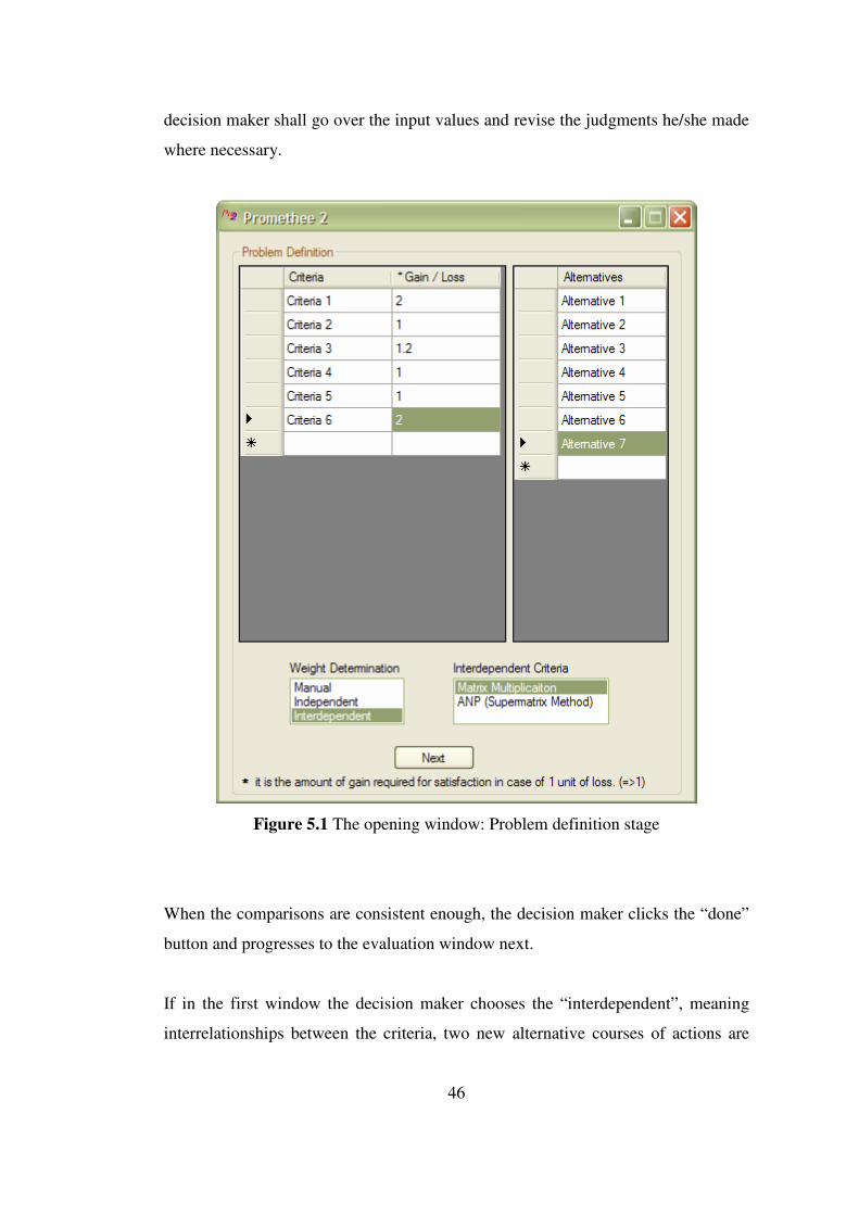
46

decision maker shall go over the input values and revise the judgments he/she made

where necessary.

Figure 5.1 The opening window: Problem definition stage

When the comparisons are consistent enough, the decision maker clicks the “done”

button and progresses to the evaluation window next.

If in the first window the decision maker chooses the “interdependent”, meaning

interrelationships between the criteria, two new alternative courses of actions are

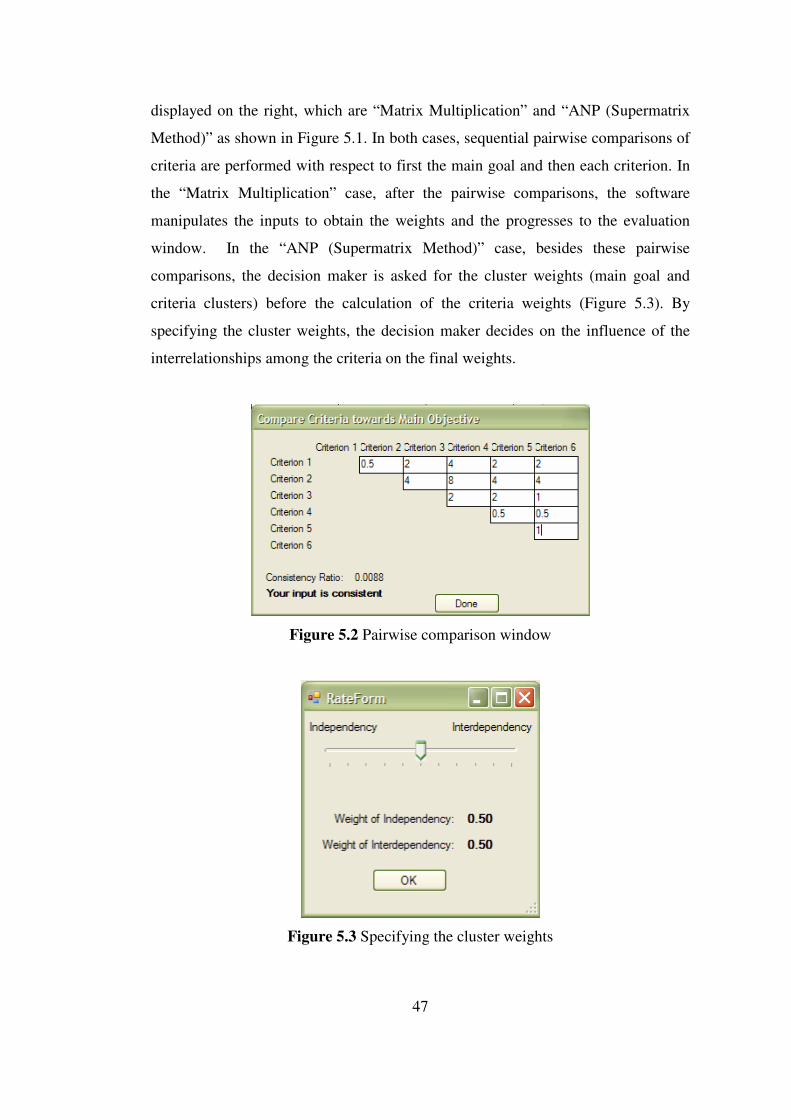
47

displayed on the right, which are “Matrix Multiplication” and “ANP (Supermatrix

Method)” as shown in Figure 5.1. In both cases, sequential pairwise comparisons of

criteria are performed with respect to first the main goal and then each criterion. In

the “Matrix Multiplication” case, after the pairwise comparisons, the software

manipulates the inputs to obtain the weights and the progresses to the evaluation

window. In the “ANP (Supermatrix Method)” case, besides these pairwise

comparisons, the decision maker is asked for the cluster weights (main goal and

criteria clusters) before the calculation of the criteria weights (Figure 5.3). By

specifying the cluster weights, the decision maker decides on the influence of the

interrelationships among the criteria on the final weights.

Figure 5.2 Pairwise comparison window

Figure 5.3 Specifying the cluster weights

48

After the weight determination stage is completed, the window illustrated in Figure

5.4 (evaluation window) appears. Here the rest of the necessary data is entered by

the decision maker. The criteria values for each alternative, the optimization type,

the preference function and the corresponding parameters for each criterion are set

by the decision maker. Now the software is ready to reveal the result, which is the

preference ranking of the alternatives.

When the “next” button is clicked, a new window appears with a table on the left

showing a square matrix of alternatives with the outranking degrees (Π1 / Π2) and

the Promethee flows (entering and leaving) (Figure 5.5). On the right, the final

ranking of the alternatives is given in the order of descending net flow values. The

net flow values, which are calculated using the entering and the leaving flow values

are also listed in the final ranking.

The algorithm of the software is illustrated with the flowchart in Figure 5.6.

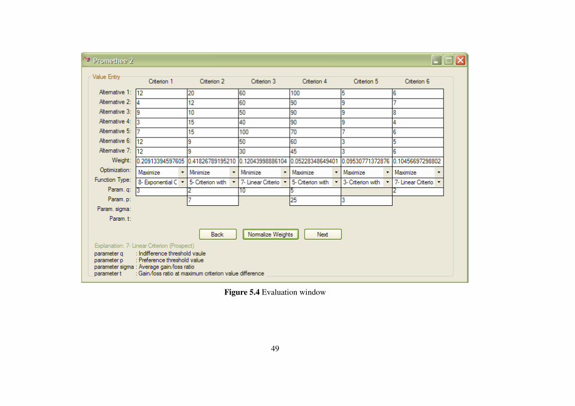
49

Figure 5.4 Evaluation window

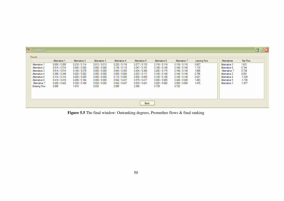
50

Figure 5.5 The final window: Outranking degrees, Promethee flows & final ranking

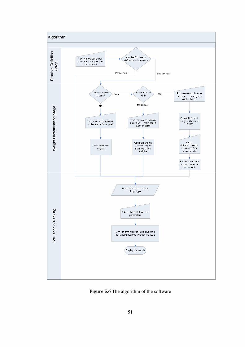
51

Figure 5.6 The algorithm of the software

52

CHAPTER 6

COMPARISON OF THE WEIGHT DETERMINATION

TECHNIQUES

The weights of the criteria have a significant effect on the solution of a MCDM

problem. In the methodology proposed in this study, alternative techniques to

specify the weights are presented and explained in detail in chapter 4. The purpose

of this chapter is to observe and analyze the differences and the variations in the

final results when alternative techniques are applied.

To observe differences on the revealed solutions of the techniques proposed in

section 4.1, they are applied on the same set of data for different cases. The

techniques are applied for 3, 6 and 9 criteria cases respectively. For each case the

weights are calculated for 5 different data sets obtained throughout a random

number generation procedure. For clearness and simplicity, eigenvectors are

generated instead of pairwise comparisons to form the comparison matrices

assuming perfect consistency.

For all the data sets, technique 1 (AHP), technique 2 (Matrix Multiplication

Method) and technique 3 (ANP – Supermatrix) are applied respectively. Since there

is the flexibility of determining the cluster weights in ANP method, ANP(w1, w2)

notation is used to indicate the cluster weights used in technique 3, where

w1: weight of the main goal cluster

w2: weight of the criteria cluster

ANP is applied with four different cluster weight set, that is ANP(1.0, 0.0),

ANP(0.5, 0.5), ANP(0.9, 0.1) and ANP(0.1, 0.9). In order to observe the impact of

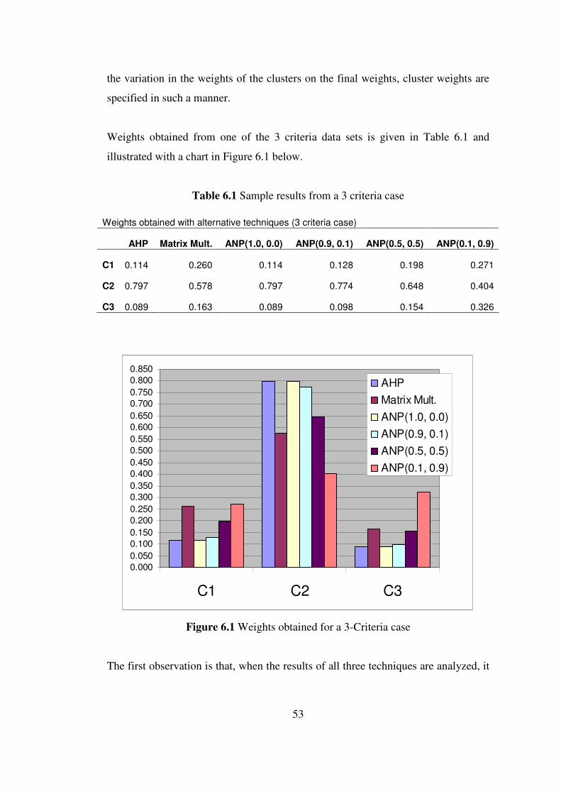
53

the variation in the weights of the clusters on the final weights, cluster weights are

specified in such a manner.

Weights obtained from one of the 3 criteria data sets is given in Table 6.1 and

illustrated with a chart in Figure 6.1 below.

Table 6.1 Sample results from a 3 criteria case

Weights obtained with alternative techniques (3 criteria case)

AHP Matrix Mult. ANP(1.0, 0.0) ANP(0.9, 0.1) ANP(0.5, 0.5) ANP(0.1, 0.9)

C1 0.114 0.260 0.114 0.128 0.198 0.271

C2 0.797 0.578 0.797 0.774 0.648 0.404

C3 0.089 0.163 0.089 0.098 0.154 0.326

0.000

0.050

0.100

0.150

0.200

0.250

0.300

0.350

0.400

0.450

0.500

0.550

0.600

0.650

0.700

0.750

0.800

0.850

C1 C2 C3

AHP

Matrix Mult.

ANP(1.0, 0.0)

ANP(0.9, 0.1)

ANP(0.5, 0.5)

ANP(0.1, 0.9)

Figure 6.1 Weights obtained for a 3-Criteria case

The first observation is that, when the results of all three techniques are analyzed, it

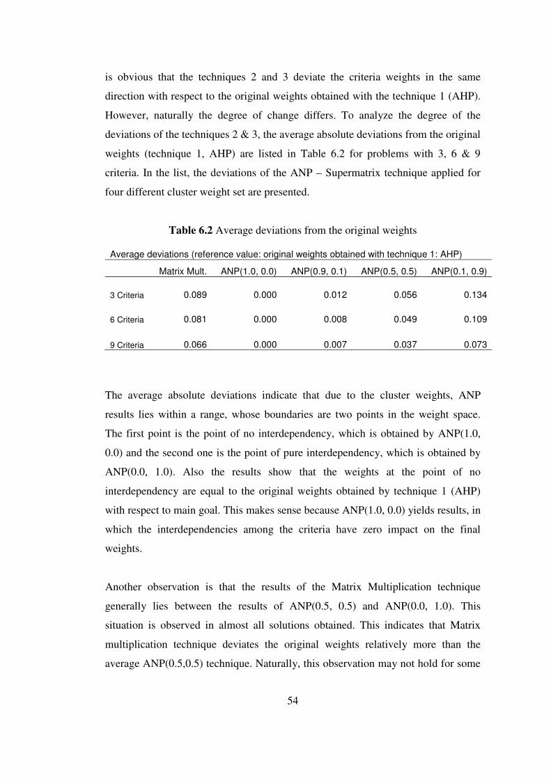
54

is obvious that the techniques 2 and 3 deviate the criteria weights in the same

direction with respect to the original weights obtained with the technique 1 (AHP).

However, naturally the degree of change differs. To analyze the degree of the

deviations of the techniques 2 & 3, the average absolute deviations from the original

weights (technique 1, AHP) are listed in Table 6.2 for problems with 3, 6 & 9

criteria. In the list, the deviations of the ANP – Supermatrix technique applied for

four different cluster weight set are presented.

Table 6.2 Average deviations from the original weights

Average deviations (reference value: original weights obtained with technique 1: AHP)

Matrix Mult. ANP(1.0, 0.0) ANP(0.9, 0.1) ANP(0.5, 0.5) ANP(0.1, 0.9)

3 Criteria 0.089 0.000 0.012 0.056 0.134

6 Criteria 0.081 0.000 0.008 0.049 0.109

9 Criteria 0.066 0.000 0.007 0.037 0.073

The average absolute deviations indicate that due to the cluster weights, ANP

results lies within a range, whose boundaries are two points in the weight space.

The first point is the point of no interdependency, which is obtained by ANP(1.0,

0.0) and the second one is the point of pure interdependency, which is obtained by

ANP(0.0, 1.0). Also the results show that the weights at the point of no

interdependency are equal to the original weights obtained by technique 1 (AHP)

with respect to main goal. This makes sense because ANP(1.0, 0.0) yields results, in

which the interdependencies among the criteria have zero impact on the final

weights.

Another observation is that the results of the Matrix Multiplication technique

generally lies between the results of ANP(0.5, 0.5) and ANP(0.0, 1.0). This

situation is observed in almost all solutions obtained. This indicates that Matrix

multiplication technique deviates the original weights relatively more than the

average ANP(0.5,0.5) technique. Naturally, this observation may not hold for some

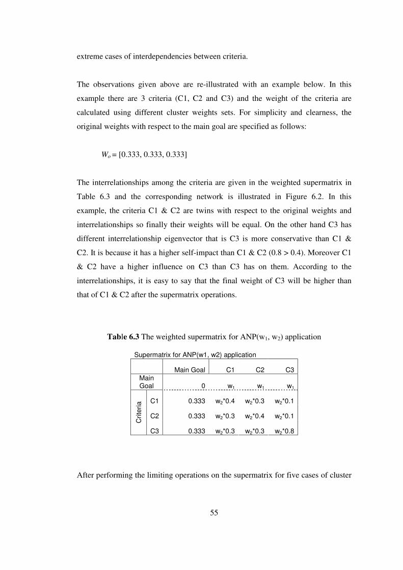
55

extreme cases of interdependencies between criteria.

The observations given above are re-illustrated with an example below. In this

example there are 3 criteria (C1, C2 and C3) and the weight of the criteria are

calculated using different cluster weights sets. For simplicity and clearness, the

original weights with respect to the main goal are specified as follows:

Wo = [0.333, 0.333, 0.333]

The interrelationships among the criteria are given in the weighted supermatrix in

Table 6.3 and the corresponding network is illustrated in Figure 6.2. In this

example, the criteria C1 & C2 are twins with respect to the original weights and

interrelationships so finally their weights will be equal. On the other hand C3 has

different interrelationship eigenvector that is C3 is more conservative than C1 &

C2. It is because it has a higher self-impact than C1 & C2 (0.8 > 0.4). Moreover C1

& C2 have a higher influence on C3 than C3 has on them. According to the

interrelationships, it is easy to say that the final weight of C3 will be higher than

that of C1 & C2 after the supermatrix operations.

Table 6.3 The weighted supermatrix for ANP(w1, w2) application

Supermatrix for ANP(w1, w2) application

Main Goal C1 C2 C3

Main Goal 0 w1 w1 w1

C1 0.333 w2*0.4 w2*0.3 w2*0.1

C2 0.333 w2*0.3 w2*0.4 w2*0.1

Crite

ria

C3 0.333 w2*0.3 w2*0.3 w2*0.8

After performing the limiting operations on the supermatrix for five cases of cluster

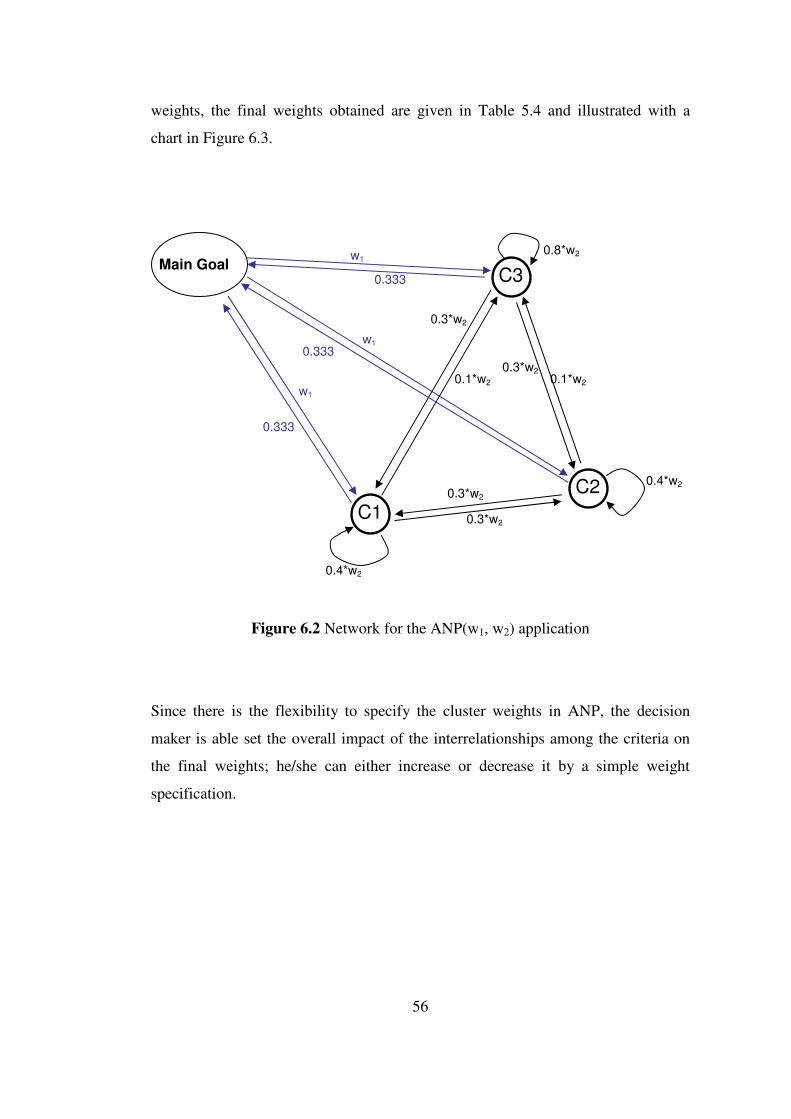
56

weights, the final weights obtained are given in Table 5.4 and illustrated with a

chart in Figure 6.3.

Figure 6.2 Network for the ANP(w1, w2) application

Since there is the flexibility to specify the cluster weights in ANP, the decision

maker is able set the overall impact of the interrelationships among the criteria on

the final weights; he/she can either increase or decrease it by a simple weight

specification.

Main Goal

C1

C2

C3

0.333

0.333

0.333

0.4*w2

0.8*w2

0.4*w2

w1

w1

0.3*w2

0.1*w2

0.3*w2

0.3*w2

0.3*w2

0.1*w2

w1

57

Table 6.4 Solutions with AHP, Matrix Mult. & ANP techniques

Final weights with alternative techniques

Technique 3: ANP (Supermatrix)

w1: 1.0 0.9 0.5 0.1 0.0

Technique 1: AHP

Technique 2: Matrix Mult. w2: 0.0 0.1 0.5 0.9 1.0

C1 0.333 0.267 0.333 0.326 0.289 0.224 0.200

C2 0.333 0.267 0.333 0.326 0.289 0.224 0.200

C3 0.333 0.466 0.333 0.348 0.423 0.552 0.600

Criteria Weights with Alternative Techniques

0

0.05

0.1

0.15

0.2

0.25

0.3

0.35

0.4

0.45

0.5

0.55

0.6

0.65

AH

P

Matr

ix M

ult.

AN

P(1

.0,

0.0

)

AN

P(0

.9,

0.1

)

AN

P(0

.5,

0.5

)

AN

P(0

.1,

0.9

)

AN

P(0

.0,

1.0

)

C1 C2 C3

Figure 6.3 Variation of the weights with alt. techniques

58

CHAPTER 7

SAMPLE SOLUTIONS

In this chapter, sample problems from different scenarios are solved using the

methodology developed. The scenarios are generated using the problem solved in a

study conducted by Wang et al. (2006). The problem is ranking of outsourcing

decisions of parts of IS functions. They treat the problem through a hybrid method

composed of AHP and Promethee II. In their hybrid method, similar to the

methodology developed in this study, AHP is used to analyze the structure of the

outsourcing problem and to determine the weights of the criteria (independent

criteria) and Promethee II is used for final ranking.

In order to observe the changes in the final ranking, each time a slight change is

made on the original problem structure. More specifically, since the new

methodology introduces techniques to handle the interdependency among criteria

and new preference functions to reflect the decision behavior of the decision maker,

modifications in accordance with these two important facts of the MCDM problems

are introduced into the sample problem.

Firstly, interdependency among criteria is introduced. The proposed alternative

techniques (Matrix Multiplication and ANP) are utilized separately to obtain two

distinct final rankings. Secondly, it is assumed that Prospect Theory best suits the

decision maker’s choice behavior for some criteria and new preference functions

are introduced and another new final ranking is obtained. Lastly, combinations of

these two situations are applied so that the problem structure became more realistic.

Towards the solutions, the author was set as the decision maker and contributed

with his judgments and evaluations where required. However, the criteria values

59

(quantitative and qualitative) kept same as the original problem, in order to observe

the differences between the methods applied. The obtained solutions for the

generated scenarios are given in Table 7.17 at the end of this chapter.

In the first section, the original problem and its solution is presented in detail

whereas in the second section the generated scenarios and their differentiations are

briefly explained. Finally in the last section the final rankings of all the solutions are

summarized with comments and discussions.

7.1 ORIGINAL PROBLEM

As mentioned before, the original problem is the ranking of outsourcing decisions

of parts of IS functions. Six criteria are defined in agreement with a group of

experts and managers and there are 5 candidate systems for outsourcing. The

criteria and the alternatives are listed in Table 7.1 and Table 7.2 respectively. The

descriptions of the criteria are as follows:

Economics

For economics (C1), the major consideration of a firm is to reduce costs of

information systems. Because the vendors have a better management skill as well as

higher productivity per employee, the costs can be reduced. Meanwhile, because of

the scale of economics vendors have invested in the hardware, software and human

resources, the cost can be reduced. Another consideration of economics is financial

flexibility. Because of outsourcing, the facilities and employee would be transferred

to the vendor side, which transform fixed costs into variable costs, resulting in

increasing financial flexibility

Resource

For resource (C2), resources include new technologies and professional workers.

The fastest and most effective way to get qualifiedworkers of IT is to outsource.

60

Outsourcing also can provide immediate access to the latest technologies with the

lead time customary in in-house development. In-house workers can learn new

technology of software management and development from the vendor [7,13,28].

Strategy

For strategy (C3), firms need to focus on their core activities and outsource non

core activities. IS outsourcing allows management to focus available IS talent on

important and strategic IT applications rather than the mundane and routine

activities. The internal operations and outsourced operations should then work in

union striving to optimize flexibility and responsiveness to customer and internal

needs, and minimize unnecessary paperwork and bureaucracy. In addition, the firms

can make strategic alliance with vendors to make up the shortage of resources.

From strategic alliances, the firm even can develop and market new products. Other

strategic consideration includes sharing risks and accelerating the time of product to

market

Risk

For risk (C4), it is rare to experience opportunities in organizational life where the

managerial actions taken to produce benefits are not associated with potential risks

either. This is most certainly the case with IS outsourcing. The risks that have to be

dealt with include: loss of core competence, loss of internal technical knowledge,

loss of flexibility, damaging the firm’s innovative capability, increasing information

services management complexity, etc. As being the factors with benefits, these risks

factors should not be ignored in outsourcing activities.

Management

For management (C5), the problems that have to be dealt with include: improving

communication problems and selfishness between IS department and operational

department, stimulating IS department to improve their performance and enhance

morale, increasing the ability of management and control of IS department, solving

the floating and scarcity of employee, keeping the flexibility to adjust department,

etc.

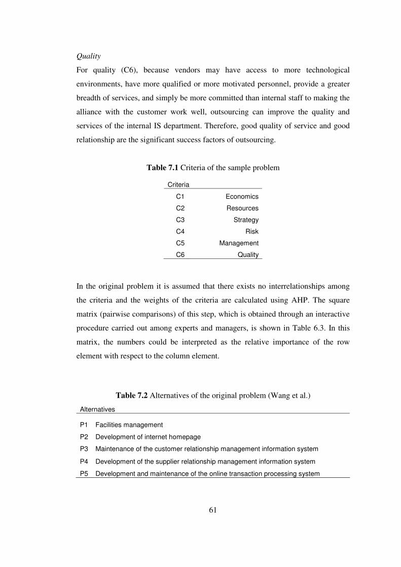
61

Quality

For quality (C6), because vendors may have access to more technological

environments, have more qualified or more motivated personnel, provide a greater

breadth of services, and simply be more committed than internal staff to making the

alliance with the customer work well, outsourcing can improve the quality and

services of the internal IS department. Therefore, good quality of service and good

relationship are the significant success factors of outsourcing.

Table 7.1 Criteria of the sample problem

In the original problem it is assumed that there exists no interrelationships among

the criteria and the weights of the criteria are calculated using AHP. The square

matrix (pairwise comparisons) of this step, which is obtained through an interactive

procedure carried out among experts and managers, is shown in Table 6.3. In this

matrix, the numbers could be interpreted as the relative importance of the row

element with respect to the column element.

Table 7.2 Alternatives of the original problem (Wang et al.)

Criteria

C1 Economics

C2 Resources

C3 Strategy

C4 Risk

C5 Management

C6 Quality

Alternatives

P1 Facilities management

P2 Development of internet homepage

P3 Maintenance of the customer relationship management information system

P4 Development of the supplier relationship management information system

P5 Development and maintenance of the online transaction processing system

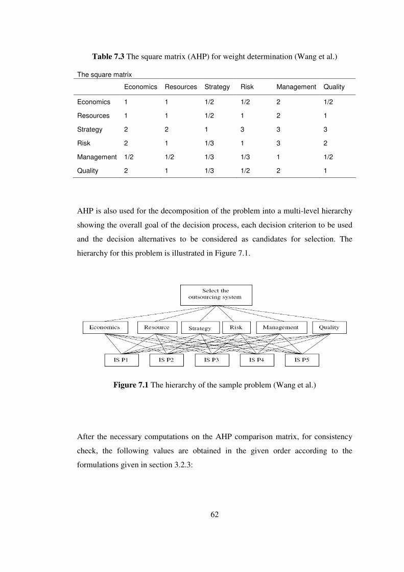
62

Table 7.3 The square matrix (AHP) for weight determination (Wang et al.)

The square matrix

Economics Resources Strategy Risk Management Quality

Economics 1 1 1/2 1/2 2 1/2

Resources 1 1 1/2 1 2 1

Strategy 2 2 1 3 3 3

Risk 2 1 1/3 1 3 2

Management 1/2 1/2 1/3 1/3 1 1/2

Quality 2 1 1/3 1/2 2 1

AHP is also used for the decomposition of the problem into a multi-level hierarchy

showing the overall goal of the decision process, each decision criterion to be used

and the decision alternatives to be considered as candidates for selection. The

hierarchy for this problem is illustrated in Figure 7.1.

Figure 7.1 The hierarchy of the sample problem (Wang et al.)

After the necessary computations on the AHP comparison matrix, for consistency

check, the following values are obtained in the given order according to the

formulations given in section 3.2.3:

63

2218.6max =λ , {highest eigenvalue where n = 6}

04436.0=CI

24.1* =CI {for n = 6}

0358.0=CR < 0.1

Since CR (consistency ratio) is less than 10 %, the evaluations made for the square

matrix are said to be consistent enough. Hence, the eigenvector corresponding to the

highest eigenvalue, i.e. the weight vector is

Wo = [0.12, 0.15, 0.33, 0.19, 0.07, 0.14]

Evaluations of the alternatives according to the criteria described above are

provided in the evaluation matrix given in Table 7.4.

For the criteria 2 to 6, a qualitative impact value was used, expressed on a

qualitative scale that is used for calculations (Judgments on a series of ordered

semantic values, which are the elements of the set {very weak, weak, common,

good, common good} is associated with a numerical value such as ranking from 1

to 5).

For the application of the Promethee II method to rank the candidate systems,

specific preference functions with the corresponding necessary parameters defined

for each criterion are listed in Table 7.5.

The problem is now ready for the implementation of the Promethee II method.

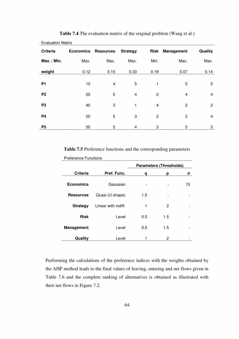
64

Table 7.4 The evaluation matrix of the original problem (Wang et al.)

Table 7.5 Preference functions and the corresponding parameters

Preference Functions

Parameters (Thresholds)

Criteria Pref. Func. q p σ

Economics Gaussian - - 15

Resources Quasi (U-shape) 1.5 - -

Strategy Linear with indiff. 1 2 -

Risk Level 0.5 1.5 -

Management Level 0.5 1.5 -

Quality Level 1 2 -

Performing the calculations of the preference indices with the weights obtained by

the AHP method leads to the final values of leaving, entering and net flows given in

Table 7.6 and the complete ranking of alternatives is obtained as illustrated with

their net flows in Figure 7.2.

Evaluation Matrix

Criteria Economics Resources Strategy Risk Management Quality

Max. / Min. Max. Max. Max. Min. Max. Max.

weight 0.12 0.15 0.33 0.19 0.07 0.14

P1 10 4 5 1 5 5

P2 25 5 4 2 4 4

P3 40 3 1 4 2 2

P4 20 5 3 2 2 4

P5 50 5 4 3 5 3

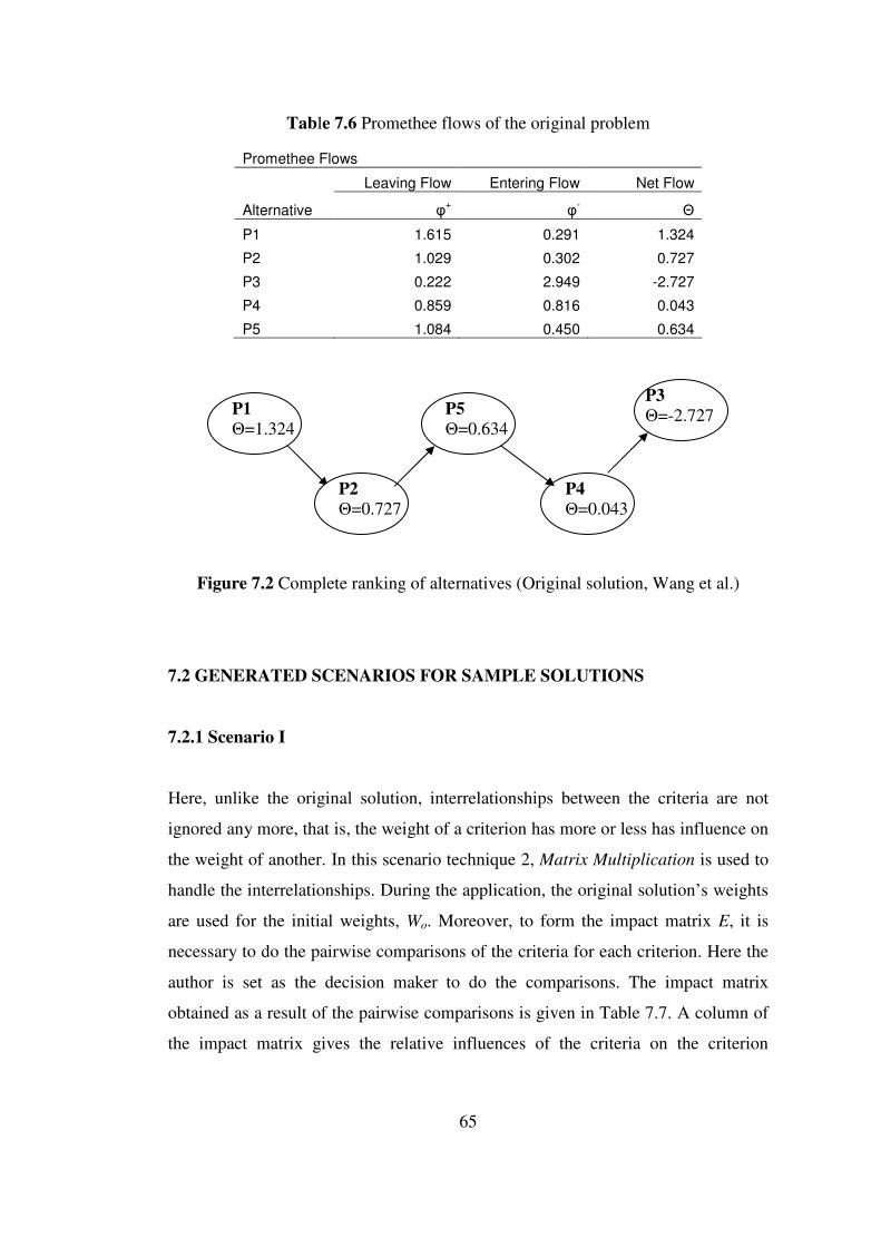
65

Table 7.6 Promethee flows of the original problem

Figure 7.2 Complete ranking of alternatives (Original solution, Wang et al.)

7.2 GENERATED SCENARIOS FOR SAMPLE SOLUTIONS

7.2.1 Scenario I

Here, unlike the original solution, interrelationships between the criteria are not

ignored any more, that is, the weight of a criterion has more or less has influence on

the weight of another. In this scenario technique 2, Matrix Multiplication is used to

handle the interrelationships. During the application, the original solution’s weights

are used for the initial weights, Wo. Moreover, to form the impact matrix E, it is

necessary to do the pairwise comparisons of the criteria for each criterion. Here the

author is set as the decision maker to do the comparisons. The impact matrix

obtained as a result of the pairwise comparisons is given in Table 7.7. A column of

the impact matrix gives the relative influences of the criteria on the criterion

Promethee Flows

Leaving Flow Entering Flow Net Flow

Alternative φ+ φ

- Θ

P1 1.615 0.291 1.324

P2 1.029 0.302 0.727

P3 0.222 2.949 -2.727

P4 0.859 0.816 0.043

P5 1.084 0.450 0.634

P1 Θ=1.324

P2 Θ=0.727

P5 Θ=0.634

P4 Θ=0.043

P3 Θ=-2.727

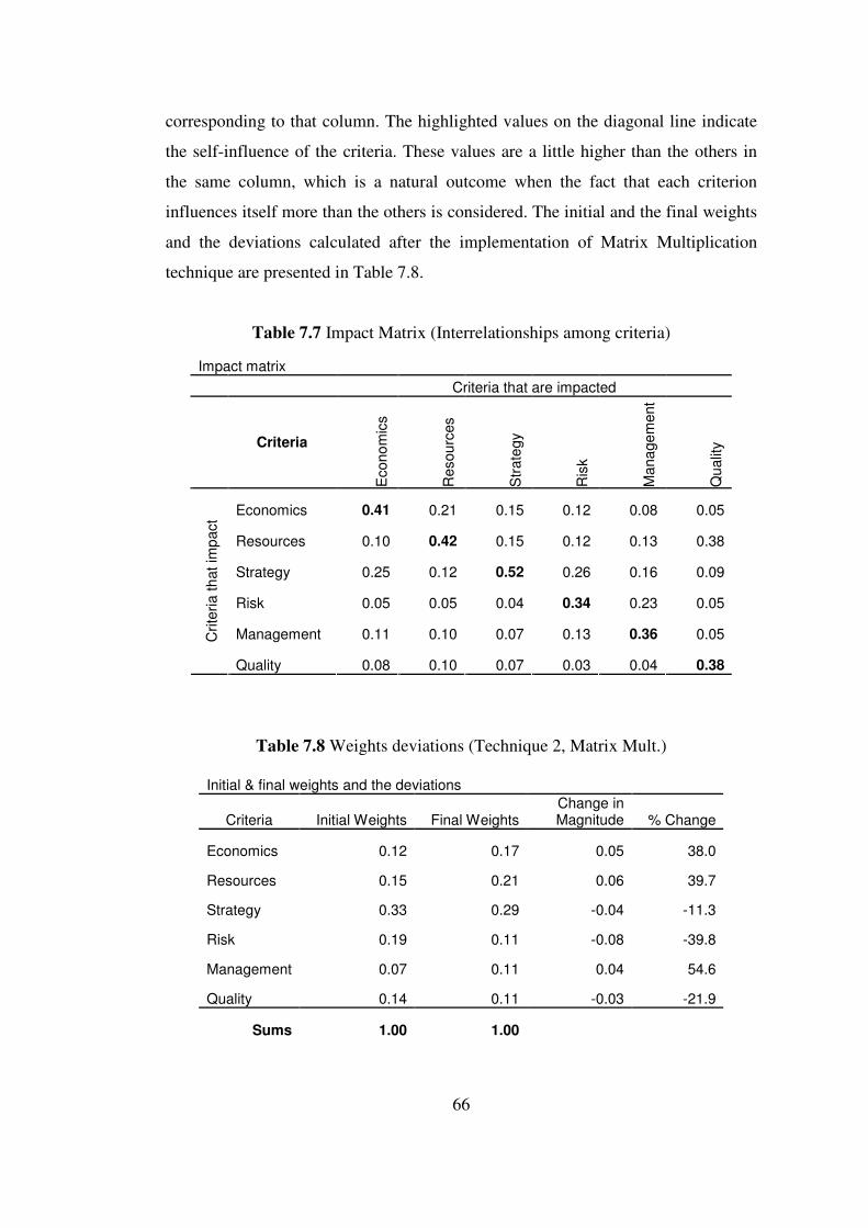
66

corresponding to that column. The highlighted values on the diagonal line indicate

the self-influence of the criteria. These values are a little higher than the others in

the same column, which is a natural outcome when the fact that each criterion

influences itself more than the others is considered. The initial and the final weights

and the deviations calculated after the implementation of Matrix Multiplication

technique are presented in Table 7.8.

Table 7.7 Impact Matrix (Interrelationships among criteria)

Impact matrix

Criteria that are impacted

Criteria

Econo

mic

s

Resourc

es

Str

ate

gy

Ris

k

Mana

ge

ment

Qualit

y

Economics 0.41 0.21 0.15 0.12 0.08 0.05

Resources 0.10 0.42 0.15 0.12 0.13 0.38

Strategy 0.25 0.12 0.52 0.26 0.16 0.09

Risk 0.05 0.05 0.04 0.34 0.23 0.05

Management 0.11 0.10 0.07 0.13 0.36 0.05 Crite

ria th

at im

pact

Quality 0.08 0.10 0.07 0.03 0.04 0.38

Table 7.8 Weights deviations (Technique 2, Matrix Mult.)

Initial & final weights and the deviations

Criteria Initial Weights Final Weights Change in Magnitude % Change

Economics 0.12 0.17 0.05 38.0

Resources 0.15 0.21 0.06 39.7

Strategy 0.33 0.29 -0.04 -11.3

Risk 0.19 0.11 -0.08 -39.8

Management 0.07 0.11 0.04 54.6

Quality 0.14 0.11 -0.03 -21.9

Sums 1.00 1.00

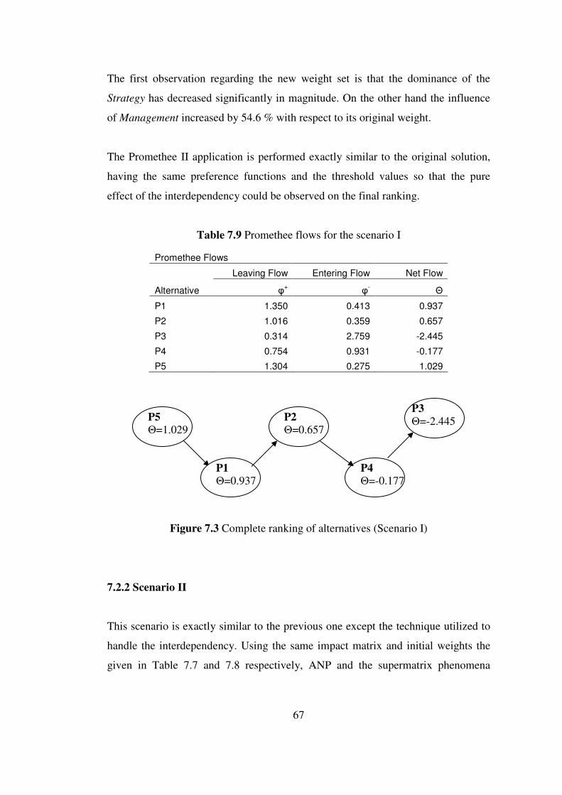
67

The first observation regarding the new weight set is that the dominance of the

Strategy has decreased significantly in magnitude. On the other hand the influence

of Management increased by 54.6 % with respect to its original weight.

The Promethee II application is performed exactly similar to the original solution,

having the same preference functions and the threshold values so that the pure

effect of the interdependency could be observed on the final ranking.

Table 7.9 Promethee flows for the scenario I

Figure 7.3 Complete ranking of alternatives (Scenario I)

7.2.2 Scenario II

This scenario is exactly similar to the previous one except the technique utilized to

handle the interdependency. Using the same impact matrix and initial weights the

given in Table 7.7 and 7.8 respectively, ANP and the supermatrix phenomena

Promethee Flows

Leaving Flow Entering Flow Net Flow

Alternative φ+ φ

- Θ

P1 1.350 0.413 0.937

P2 1.016 0.359 0.657

P3 0.314 2.759 -2.445

P4 0.754 0.931 -0.177

P5 1.304 0.275 1.029

P5 Θ=1.029

P1 Θ=0.937

P2 Θ=0.657

P4 Θ=-0.177

P3 Θ=-2.445

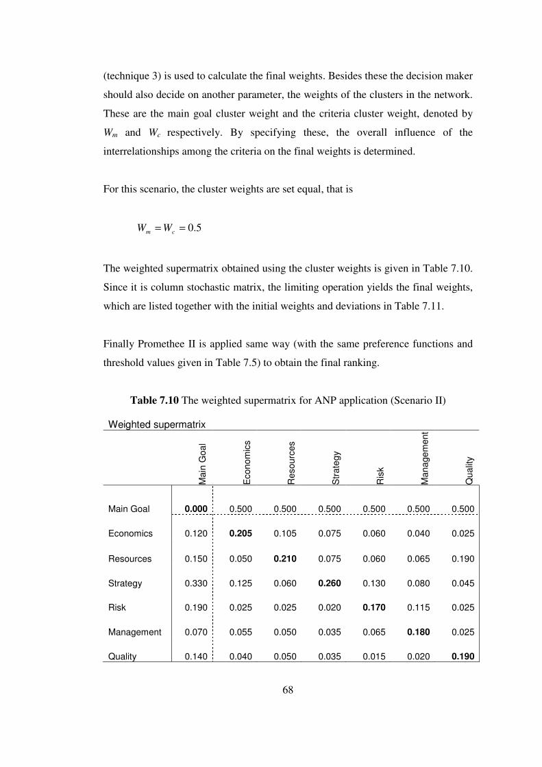
68

(technique 3) is used to calculate the final weights. Besides these the decision maker

should also decide on another parameter, the weights of the clusters in the network.

These are the main goal cluster weight and the criteria cluster weight, denoted by

Wm and Wc respectively. By specifying these, the overall influence of the

interrelationships among the criteria on the final weights is determined.

For this scenario, the cluster weights are set equal, that is

5.0== cm WW

The weighted supermatrix obtained using the cluster weights is given in Table 7.10.

Since it is column stochastic matrix, the limiting operation yields the final weights,

which are listed together with the initial weights and deviations in Table 7.11.

Finally Promethee II is applied same way (with the same preference functions and

threshold values given in Table 7.5) to obtain the final ranking.

Table 7.10 The weighted supermatrix for ANP application (Scenario II)

Weighted supermatrix

Main

Goa

l

Econo

mic

s

Resourc

es

Str

ate

gy

Ris

k

Mana

ge

ment

Qualit

y

Main Goal 0.000 0.500 0.500 0.500 0.500 0.500 0.500

Economics 0.120 0.205 0.105 0.075 0.060 0.040 0.025

Resources 0.150 0.050 0.210 0.075 0.060 0.065 0.190

Strategy 0.330 0.125 0.060 0.260 0.130 0.080 0.045

Risk 0.190 0.025 0.025 0.020 0.170 0.115 0.025

Management 0.070 0.055 0.050 0.035 0.065 0.180 0.025

Quality 0.140 0.040 0.050 0.035 0.015 0.020 0.190

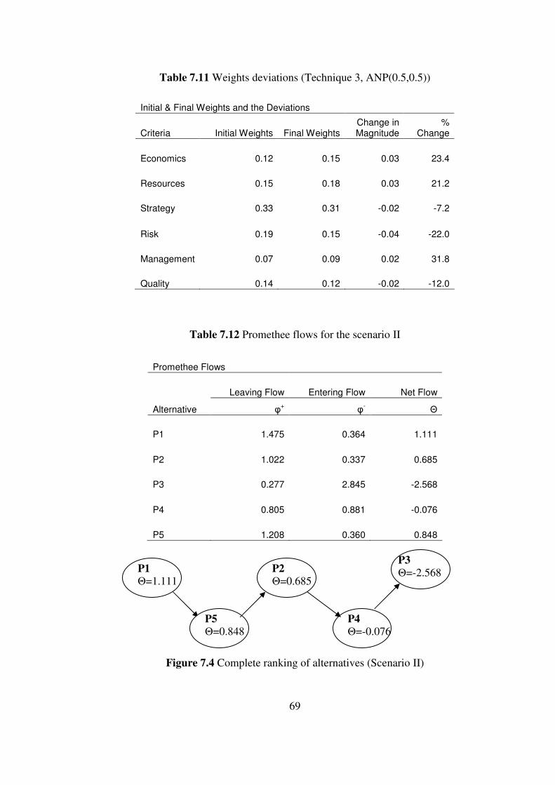
69

Table 7.11 Weights deviations (Technique 3, ANP(0.5,0.5))

Initial & Final Weights and the Deviations

Criteria Initial Weights Final Weights Change in Magnitude

% Change

Economics 0.12 0.15 0.03 23.4

Resources 0.15 0.18 0.03 21.2

Strategy 0.33 0.31 -0.02 -7.2

Risk 0.19 0.15 -0.04 -22.0

Management 0.07 0.09 0.02 31.8

Quality 0.14 0.12 -0.02 -12.0

Table 7.12 Promethee flows for the scenario II

Figure 7.4 Complete ranking of alternatives (Scenario II)

Promethee Flows

Leaving Flow Entering Flow Net Flow

Alternative φ+ φ

- Θ

P1 1.475 0.364 1.111

P2 1.022 0.337 0.685

P3 0.277 2.845 -2.568

P4 0.805 0.881 -0.076

P5 1.208 0.360 0.848

P1 Θ=1.111

P5 Θ=0.848

P2 Θ=0.685

P4 Θ=-0.076

P3 Θ=-2.568

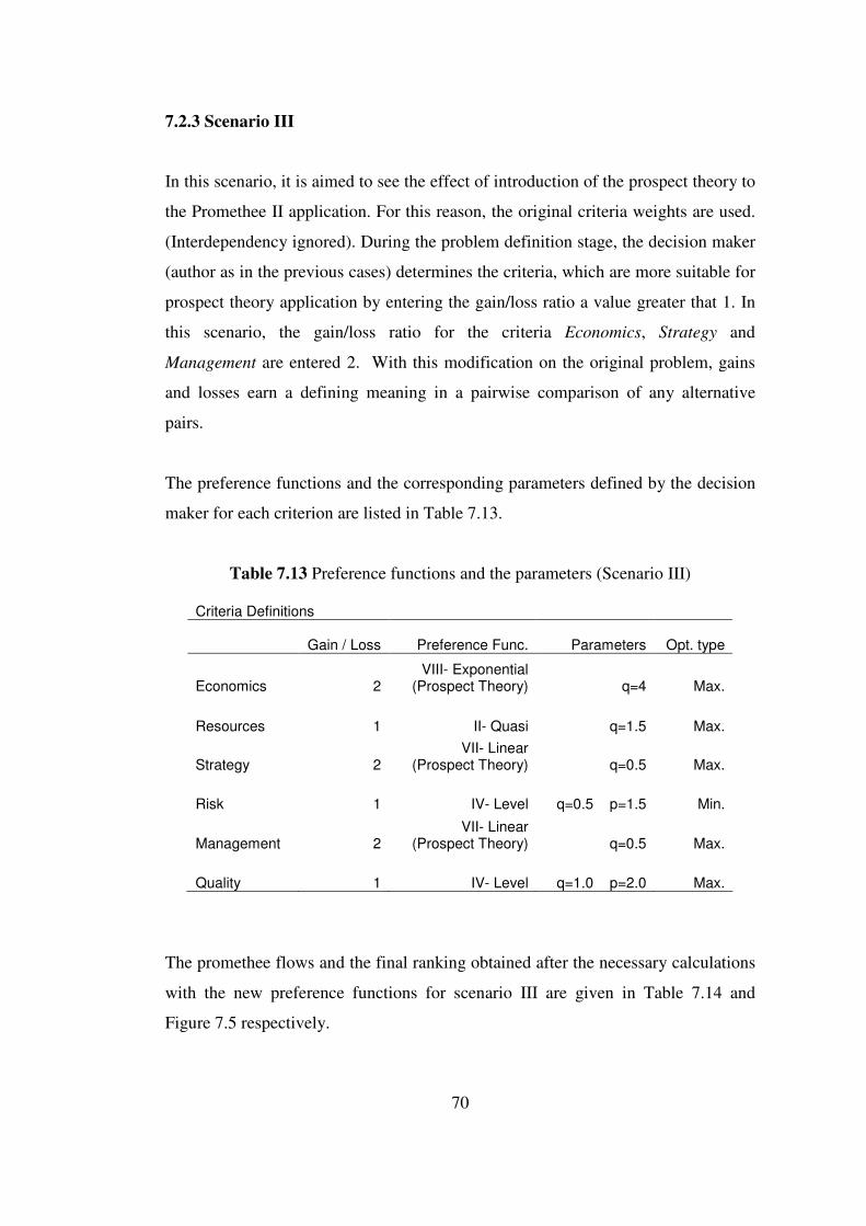
70

7.2.3 Scenario III

In this scenario, it is aimed to see the effect of introduction of the prospect theory to

the Promethee II application. For this reason, the original criteria weights are used.

(Interdependency ignored). During the problem definition stage, the decision maker

(author as in the previous cases) determines the criteria, which are more suitable for

prospect theory application by entering the gain/loss ratio a value greater that 1. In

this scenario, the gain/loss ratio for the criteria Economics, Strategy and

Management are entered 2. With this modification on the original problem, gains

and losses earn a defining meaning in a pairwise comparison of any alternative

pairs.

The preference functions and the corresponding parameters defined by the decision

maker for each criterion are listed in Table 7.13.

Table 7.13 Preference functions and the parameters (Scenario III)

Criteria Definitions

Gain / Loss Preference Func. Parameters Opt. type

Economics 2 VIII- Exponential

(Prospect Theory) q=4 Max.

Resources 1 II- Quasi q=1.5 Max.

Strategy 2 VII- Linear

(Prospect Theory) q=0.5 Max.

Risk 1 IV- Level q=0.5 p=1.5 Min.

Management 2 VII- Linear

(Prospect Theory) q=0.5 Max.

Quality 1 IV- Level q=1.0 p=2.0 Max.

The promethee flows and the final ranking obtained after the necessary calculations

with the new preference functions for scenario III are given in Table 7.14 and

Figure 7.5 respectively.

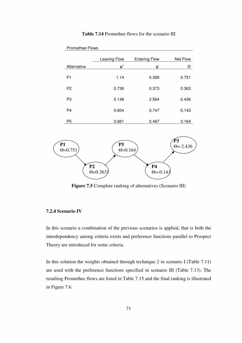
71

Table 7.14 Promethee flows for the scenario III

Figure 7.5 Complete ranking of alternatives (Scenario III)

7.2.4 Scenario IV

In this scenario a combination of the previous scenarios is applied, that is both the

interdependency among criteria exists and preference functions parallel to Prospect

Theory are introduced for some criteria.

In this solution the weights obtained through technique 2 in scenario I (Table 7.11)

are used with the preference functions specified in scenario III (Table 7.13). The

resulting Promethee flows are listed in Table 7.15 and the final ranking is illustrated

in Figure 7.6.

Promethee Flows

Leaving Flow Entering Flow Net Flow

Alternative φ+ φ

- Θ

P1 1.14 0.389 0.751

P2 0.736 0.373 0.363

P3 0.148 2.584 -2.436

P4 0.604 0.747 -0.143

P5 0.661 0.497 0.164

P1 Θ=0.751

P2 Θ=0.3631

P5 Θ=0.164

P4 Θ=-0.143

P3 Θ=-2.436

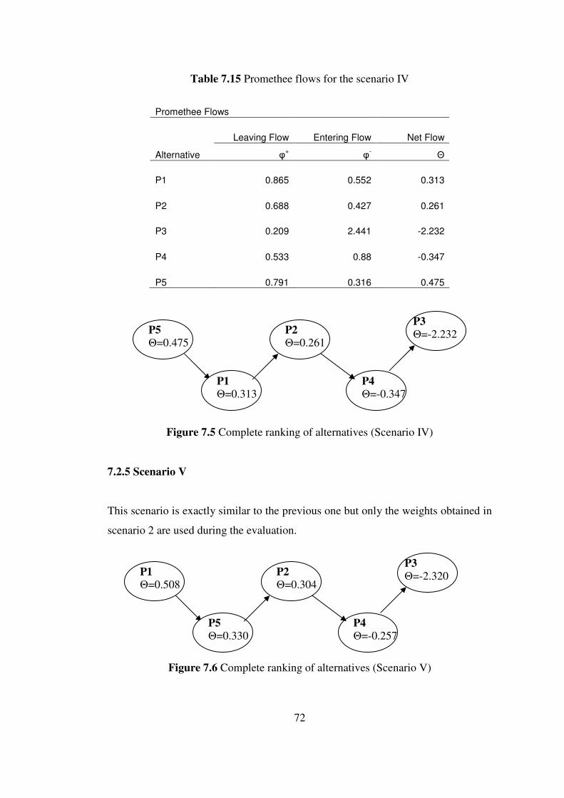
72

Table 7.15 Promethee flows for the scenario IV

Figure 7.5 Complete ranking of alternatives (Scenario IV)

7.2.5 Scenario V

This scenario is exactly similar to the previous one but only the weights obtained in

scenario 2 are used during the evaluation.

Figure 7.6 Complete ranking of alternatives (Scenario V)

Promethee Flows

Leaving Flow Entering Flow Net Flow

Alternative φ+ φ

- Θ

P1 0.865 0.552 0.313

P2 0.688 0.427 0.261

P3 0.209 2.441 -2.232

P4 0.533 0.88 -0.347

P5 0.791 0.316 0.475

P1 Θ=0.508

P5 Θ=0.330

P2 Θ=0.304

P4 Θ=-0.257

P3 Θ=-2.320

P5 Θ=0.475

P1 Θ=0.313

P2 Θ=0.261

P4 Θ=-0.347

P3 Θ=-2.232

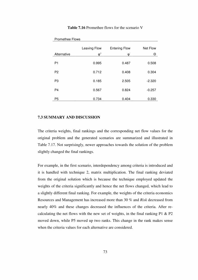
73

Table 7.16 Promethee flows for the scenario V

7.3 SUMMARY AND DISCUSSION

The criteria weights, final rankings and the corresponding net flow values for the

original problem and the generated scenarios are summarized and illustrated in

Table 7.17. Not surprisingly, newer approaches towards the solution of the problem

slightly changed the final rankings.

For example, in the first scenario, interdependency among criteria is introduced and

it is handled with technique 2, matrix multiplication. The final ranking deviated

from the original solution which is because the technique employed updated the

weights of the criteria significantly and hence the net flows changed, which lead to

a slightly different final ranking. For example, the weights of the criteria economics

Resources and Management has increased more than 30 % and Risk decreased from

nearly 40% and these changes decreased the influences of the criteria. After re-

calculating the net flows with the new set of weights, in the final ranking P1 & P2

moved down, while P5 moved up two ranks. This change in the rank makes sense

when the criteria values for each alternative are considered.

Promethee Flows

Leaving Flow Entering Flow Net Flow

Alternative φ+ φ

- Θ

P1 0.995 0.487 0.508

P2 0.712 0.408 0.304

P3 0.185 2.505 -2.320

P4 0.567 0.824 -0.257

P5 0.734 0.404 0.330

74

Scenario II, where technique 3 (ANP - Supermatrix) is utilized with equal cluster

weights (ANP(0.5, 0.5)), revealed a final ranking that is the intersection of the

original solution and the scenario I. This outcome is reasonable because the

deviations of the weights are less than scenario I and so the net flows deviated less.

For the scenarios II, IV and V, preference functions representing Prospect Theory

properties are introduced for some criteria. The problem is solved in scenario II, IV

and V with the criteria weights of the original solution, scenario I and scenario II

respectively. Surprisingly, the introduction of Prospect Theory did not change the

rankings due to the relatively small changes in the net flow values. Therefore it can

be concluded that the deviation in the criteria weights contributes more to the final

rankings rather than the introduction of Prospect Theory.

All in all, the sample solutions obtained above prove that the kind of approach to

such discrete MCDM problems might be very much determining towards the

solution, in other words if not thoroughly analyzed or digested, some simplifying

assumptions, like ignoring the interdependencies among the criteria may obviously

lead to undesired rankings.

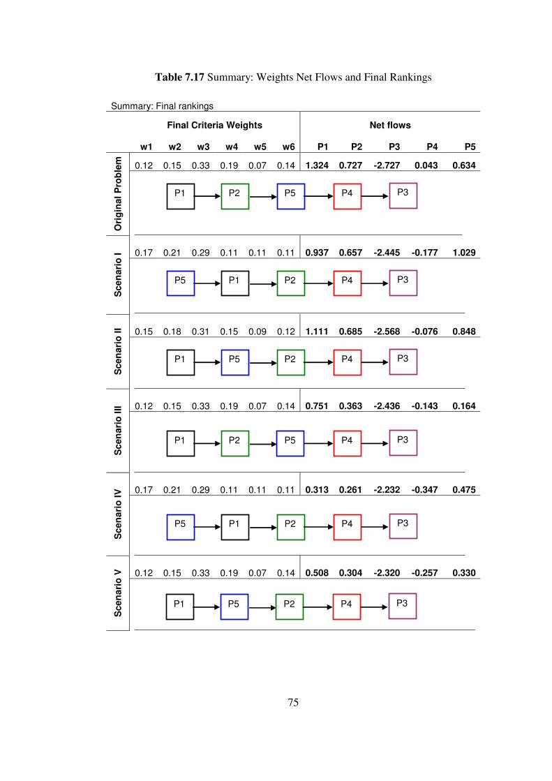
75

Table 7.17 Summary: Weights Net Flows and Final Rankings

Summary: Final rankings

Final Criteria Weights Net flows

w1 w2 w3 w4 w5 w6 P1 P2 P3 P4 P5

0.12 0.15 0.33 0.19 0.07 0.14 1.324 0.727 -2.727 0.043 0.634

Ori

gin

al

Pro

ble

m

0.17 0.21 0.29 0.11 0.11 0.11 0.937 0.657 -2.445 -0.177 1.029

Scen

ari

o I

0.15 0.18 0.31 0.15 0.09 0.12 1.111 0.685 -2.568 -0.076 0.848

Scen

ari

o I

I

0.12 0.15 0.33 0.19 0.07 0.14 0.751 0.363 -2.436 -0.143 0.164

Scen

ari

o I

II

0.17 0.21 0.29 0.11 0.11 0.11 0.313 0.261 -2.232 -0.347 0.475

Scen

ari

o I

V

0.12 0.15 0.33 0.19 0.07 0.14 0.508 0.304 -2.320 -0.257 0.330

Scen

ari

o V

P1 P2 P5 P4 P3

P5 P1 P2 P4 P3

P1 P5 P2 P4 P3

P5 P1 P2 P4 P3

P1 P5 P2 P4 P3

P1 P2 P5 P4 P3

76

CHAPTER 8

SAMPLE APPLICATION: RANKING THE UNIVERSITIES

In this chapter, a sample application of the methodology developed in this study is

performed. The applied problem is the ranking of top 101 universities around the

world within the context of 6 criteria. The problem data is obtained from the

ranking study performed in the Institute of Higher Education, Shanghai Jiao Tong

University. Using the alternative techniques, three different criteria weight set is

obtained and rankings are obtained using the software developed. At the end of this

chapter, a comparison study conducted among the original ranking and the new

rankings is presented. All the rankings obtained are given in Appendix A.2.

8.1 THE ORIGINAL RANKING STUDY

The universities are ranked by several indicators of academic or research

performance, including alumni and staff winning Nobel Prizes and Fields Medals,

highly cited researchers, articles published in Nature and Science, articles indexed

in major citation indices, and the per capita academic performance of an institution.

The data used during ranking and the sources for these data are provided in the

Appendix A.1 and A.2 respectively. For each criterion, the highest scoring

institution is assigned a score of 100, and other institutions are calculated as a

percentage of the top score. The distribution of data for each criterion is examined

for any significant distorting effect; standard statistical techniques are used to adjust

the criteria if necessary.

77

Scores for every criteria are weighted as given in Table 8.1 to arrive at a final

overall score for an institution. The highest scoring institution is assigned a score of

100, and other institutions are calculated as a percentage of the top score. An

institution's rank reflects the number of institutions that sit above it.

The definitions of the 6 criteria that are used in the problem are as follows:

1. Alumni

The total number of the alumni of an institution winning Nobel Prizes and

Fields Medals. Alumni are defined as those who obtain bachelor, Master's or

doctoral degrees from the institution. Different weights are set according to the

periods of obtaining degrees. The weight is 100% for alumni obtaining degrees

in 1991-2000, 90% for alumni obtaining degrees in 1981-1990, 80% for alumni

obtaining degrees in 1971-1980, and so on, and finally 10% for alumni

obtaining degrees in 1901-1910. If a person obtains more than one degrees from

an institution, the institution is considered once only.

2. Awards

The total number of the staff of an institution winning Nobel prizes in physics,

chemistry, medicine and economics and Fields Medal in mathematics. Staff is

defined as those who work at an institution at the time of winning the prize.

Different weights are set according to the periods of winning the prizes. The

weight is 100% for winners in 2001-2005, 90% for winners in 1991-2000, 80%

for winners in 1981-1990, 70% for winners in 1971-1980, and so on, and finally

10% for winners in 1911-1920. If a winner is affiliated with more than one

institution, each institution is assigned the reciprocal of the number of

institutions. For Nobel prizes, if a prize is shared by more than one person,

78

weights are set for winners according to their proportion of the prize.

3. HiCi

The number of highly cited researchers in broad subject categories in life

sciences, medicine, physical sciences, engineering and social sciences. These

individuals are the most highly cited within each category. The definition of

categories and detailed procedures can be found at the website of Institute of

Scientific information.

4. N&S

The number of articles published in Nature and Science between 2001 and

2005. To distinguish the order of author affiliation, a weight of 100% is

assigned for corresponding author affiliation, 50% for first author affiliation

(second author affiliation if the first author affiliation is the same as

corresponding author affiliation), 25% for the next author affiliation, and 10%

for other author affiliations. Only publications of article type are considered.

5. SCI

Total number of articles indexed in Science Citation Index-expanded and Social

Science Citation Index in 2005. Only publications of article type are considered.

When calculating the total number of articles of an institution, a special weight

of two was introduced for articles indexed in Social Science Citation Index.

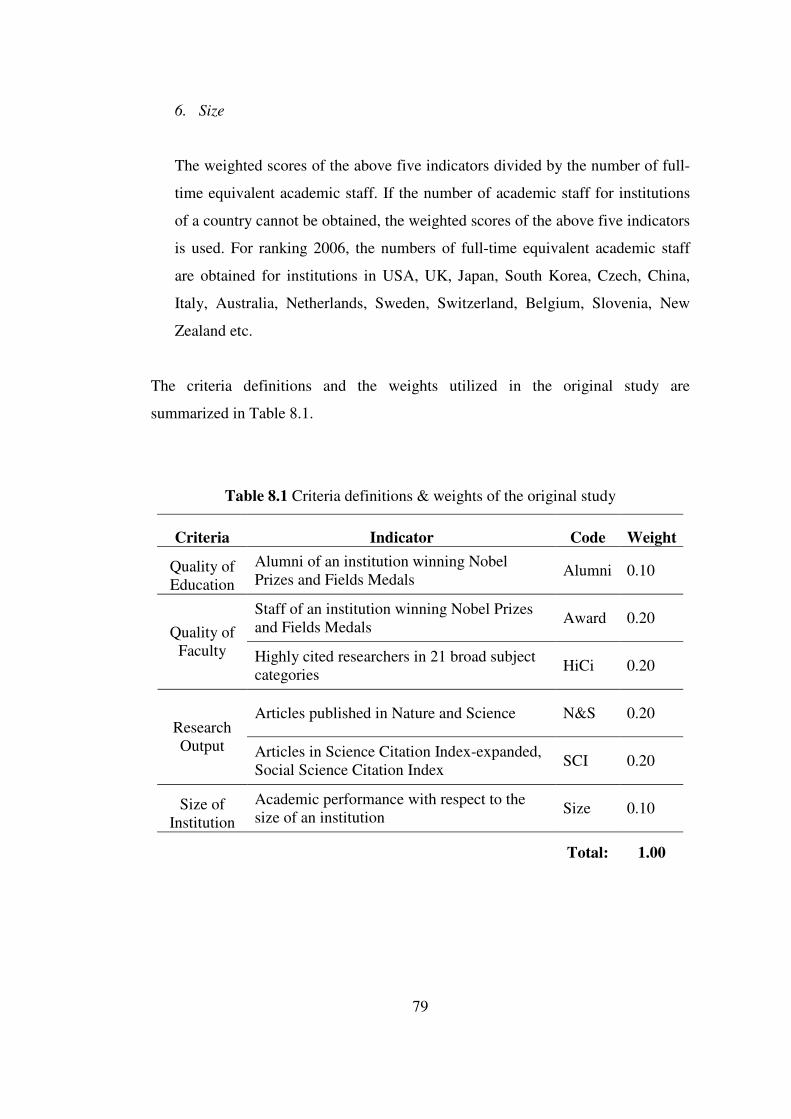
79

6. Size

The weighted scores of the above five indicators divided by the number of full-

time equivalent academic staff. If the number of academic staff for institutions

of a country cannot be obtained, the weighted scores of the above five indicators

is used. For ranking 2006, the numbers of full-time equivalent academic staff

are obtained for institutions in USA, UK, Japan, South Korea, Czech, China,

Italy, Australia, Netherlands, Sweden, Switzerland, Belgium, Slovenia, New

Zealand etc.

The criteria definitions and the weights utilized in the original study are

summarized in Table 8.1.

Table 8.1 Criteria definitions & weights of the original study

Criteria Indicator Code Weight

Quality of Education

Alumni of an institution winning Nobel Prizes and Fields Medals

Alumni 0.10

Staff of an institution winning Nobel Prizes and Fields Medals

Award 0.20 Quality of

Faculty Highly cited researchers in 21 broad subject categories

HiCi 0.20

Articles published in Nature and Science N&S 0.20 Research Output Articles in Science Citation Index-expanded,

Social Science Citation Index SCI 0.20

Size of Institution

Academic performance with respect to the size of an institution

Size 0.10

Total: 1.00

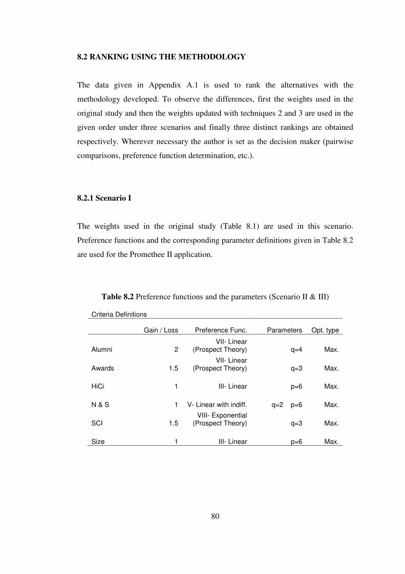
80

8.2 RANKING USING THE METHODOLOGY

The data given in Appendix A.1 is used to rank the alternatives with the

methodology developed. To observe the differences, first the weights used in the

original study and then the weights updated with techniques 2 and 3 are used in the

given order under three scenarios and finally three distinct rankings are obtained

respectively. Wherever necessary the author is set as the decision maker (pairwise

comparisons, preference function determination, etc.).

8.2.1 Scenario I

The weights used in the original study (Table 8.1) are used in this scenario.

Preference functions and the corresponding parameter definitions given in Table 8.2

are used for the Promethee II application.

Table 8.2 Preference functions and the parameters (Scenario II & III)

Criteria Definitions

Gain / Loss Preference Func. Parameters Opt. type

Alumni 2 VII- Linear

(Prospect Theory) q=4 Max.

Awards 1.5 VII- Linear

(Prospect Theory) q=3 Max.

HiCi 1 III- Linear p=6 Max.

N & S 1 V- Linear with indiff. q=2 p=6 Max.

SCI 1.5 VIII- Exponential

(Prospect Theory) q=3 Max.

Size 1 III- Linear p=6 Max.

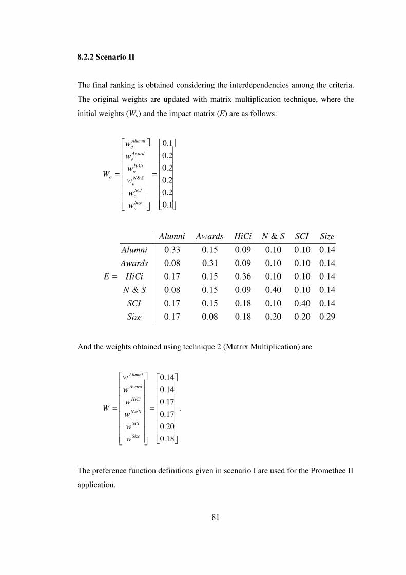
81

8.2.2 Scenario II

The final ranking is obtained considering the interdependencies among the criteria.

The original weights are updated with matrix multiplication technique, where the

initial weights (Wo) and the impact matrix (E) are as follows:

=

=

1.0

2.0

2.0

2.0

2.0

1.0

&

Size

o

SCI

o

SN

o

HiCi

o

Award

o

Alumni

o

o

w

w

w

w

w

w

W

29.020.020.018.008.017.0

14.040.010.018.015.017.0

14.010.040.009.015.008.0&

14.010.010.036.015.017.0

14.010.010.009.031.008.0

14.010.010.009.015.033.0

&

Size

SCI

SN

HiCi

Awards

Alumni

SizeSCISNHiCiAwardsAlumni

E =

And the weights obtained using technique 2 (Matrix Multiplication) are

=

=

18.0

20.0

17.0

17.0

14.0

14.0

&

Size

SCI

SN

HiCi

Award

Alumni

w

w

w

w

w

w

W .

The preference function definitions given in scenario I are used for the Promethee II

application.

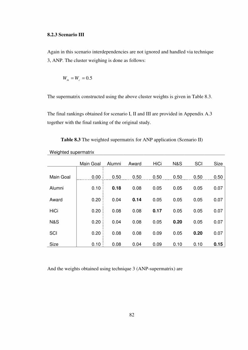
82

8.2.3 Scenario III

Again in this scenario interdependencies are not ignored and handled via technique

3, ANP. The cluster weighing is done as follows:

5.0== cm WW

The supermatrix constructed using the above cluster weights is given in Table 8.3.

The final rankings obtained for scenario I, II and III are provided in Appendix A.3

together with the final ranking of the original study.

Table 8.3 The weighted supermatrix for ANP application (Scenario II)

Weighted supermatrix

Main Goal Alumni Award HiCi N&S SCI Size

Main Goal 0.00 0.50 0.50 0.50 0.50 0.50 0.50

Alumni 0.10 0.18 0.08 0.05 0.05 0.05 0.07

Award 0.20 0.04 0.14 0.05 0.05 0.05 0.07

HiCi 0.20 0.08 0.08 0.17 0.05 0.05 0.07

N&S 0.20 0.04 0.08 0.05 0.20 0.05 0.07

SCI 0.20 0.08 0.08 0.09 0.05 0.20 0.07

Size 0.10 0.08 0.04 0.09 0.10 0.10 0.15

And the weights obtained using technique 3 (ANP-supermatrix) are

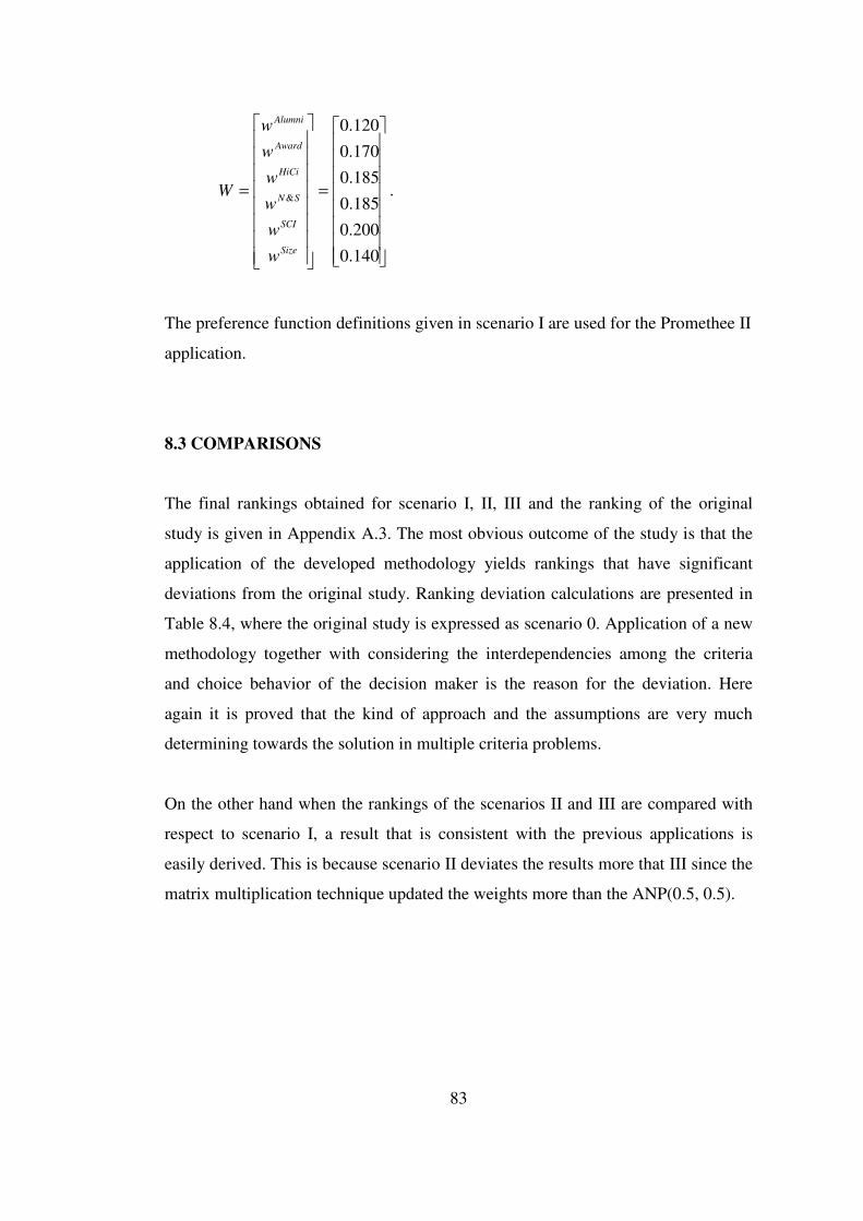
83

=

=

140.0

200.0

185.0

185.0

170.0

120.0

&

Size

SCI

SN

HiCi

Award

Alumni

w

w

w

w

w

w

W .

The preference function definitions given in scenario I are used for the Promethee II

application.

8.3 COMPARISONS

The final rankings obtained for scenario I, II, III and the ranking of the original

study is given in Appendix A.3. The most obvious outcome of the study is that the

application of the developed methodology yields rankings that have significant

deviations from the original study. Ranking deviation calculations are presented in

Table 8.4, where the original study is expressed as scenario 0. Application of a new

methodology together with considering the interdependencies among the criteria

and choice behavior of the decision maker is the reason for the deviation. Here

again it is proved that the kind of approach and the assumptions are very much

determining towards the solution in multiple criteria problems.

On the other hand when the rankings of the scenarios II and III are compared with

respect to scenario I, a result that is consistent with the previous applications is

easily derived. This is because scenario II deviates the results more that III since the

matrix multiplication technique updated the weights more than the ANP(0.5, 0.5).

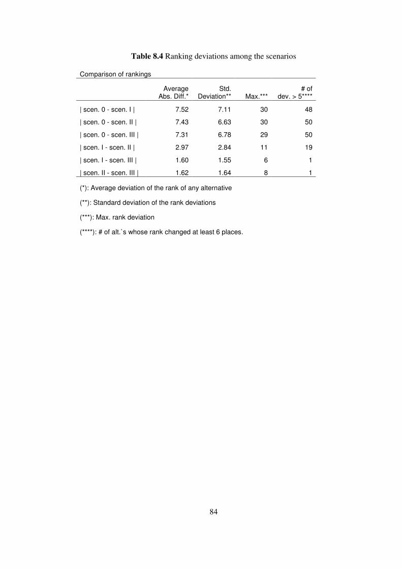
84

Table 8.4 Ranking deviations among the scenarios

Comparison of rankings

Average

Abs. Diff.* Std.

Deviation** Max.*** # of

dev. > 5****

| scen. 0 - scen. I | 7.52 7.11 30 48

| scen. 0 - scen. II | 7.43 6.63 30 50

| scen. 0 - scen. III | 7.31 6.78 29 50

| scen. I - scen. II | 2.97 2.84 11 19

| scen. I - scen. III | 1.60 1.55 6 1

| scen. II - scen. III | 1.62 1.64 8 1

(*): Average deviation of the rank of any alternative

(**): Standard deviation of the rank deviations

(***): Max. rank deviation

(****): # of alt.`s whose rank changed at least 6 places.

85

CONCLUSION

In this study, a methodology aiming to rank the alternatives in a discrete MCDM

problem is developed and proposed. It is constructed upon the basis of the well

known outranking method Promethee II. Alternative techniques are proposed for

the determination of the criteria weights and new preference functions that

incorporate the Prospect Theory into Promethee are suggested.

In discrete MCDM, there have been various methodologies developed based on the

Promethee family methods as given in chapter one. This study differs with its two

aspects. First is the way it handles the determination of the criteria weights and the

second is its approach to incorporate the choice behavior of the decision maker.

Due to the alternative techniques to specify the criteria weights, decision maker is

not restricted to a single method. He/She can either choose to incorporate the

interdependencies between the criteria and perform the calculations according to

that or ignore them. However, the two courses of actions, ignoring and not ignoring

the interdependencies among the criteria, both have some disadvantages. When the

calculations are performed without considering the interdependencies, the resulting

weight set does not reflect the reality, in other words, the contribution of the

interdependencies is totally disregarded and the existence of a criterion has no

influence on the weights of the others. For this reason, the independent criteria

assumption, which has been the dominant approach in MCDM applications and

researches, has a negative influence while modeling the problem. On the other

hand, it is not an easy process to calculate the weights with interdependency. In the

study, two alternative techniques are proposed to handle the interdependency, which

are the Matrix Multiplication technique and the ANP (supermatrix) technique. In

both there is the necessity to make the pairwise comparisons of all the criteria pairs

with respect to each criterion to obtain the relative influences between the criteria,

86

which is represented with impact matrix. Suppose there are n criteria, then the

impact matrix is an n x n matrix. The eigenvector in each column of the impact

matrix represent the relative influence on the parent criterion (the one

corresponding to that column) of the criteria. The eigenvectors are obtained through

a pairwise comparison process of AHP according to Saaty`s 1-9 scale. For each

eigenvector, (n-1)*(n-2)/2 comparisons are necessary. For the whole problem, the

total number of comparisons (only for interdependency) is n*(n-1)*(n-2)/2, which is

in the order of n3. In other words, the number of comparisons increases rapidly with

the criteria number. Moreover, it is a more difficult task to be consistent during the

pairwise comparisons when n is large. The vast number of criteria in a problem

could also be handled by grouping them into sub-clusters and the problem could be

solved by Matrix Manipulation (Saaty, 1996), constructing multi-level hierarchy

instead of single level.

One other important feature of the methodology developed is that it can manipulate

the choice behavior of the decision maker with a simple interaction by asking a

single question during the construction of the problem. This may seem to be a very

insufficient way to model the decision behavior; however, one must note that there

are yet no methods which are commonly accepted to model the decision behavior of

the decision maker and there are still researches going on to obtain the preference

function of the decision maker within the context of Decision Theory (Korhonen et

al. 1990, Salminen 1994, Karasakal et al. 2005). Considering this, simply the

method given in this study is proposed instead of a sophisticated one.

According to the answer given by the decision maker to the question asked in the

beginning of the methodology, two different sets of preference functions are

proposed as given in chapter 3. The first set is composed of conventional functions

suggested with Promethee by Brans et al (1986). In the second set, there are two

new preference functions that incorporate the Prospect Theory (Kahneman and

Tversky, 1979). According to the definition of the prospect theory, the preference

function is steeper for losses than for gains in the new preference functions. The

87

preference function is updated according to the answer given by the decision maker,

so that it yields less for the gains than losses.

All in all, the main characteristic of the methodology developed is its flexibility that

there exist alternative courses of actions during the criteria weights determination

stage and the specification of the preference functions with respect to each criterion.

The work presented in this study may be improved with respect to many different

perspectives as listed below:

• Within organizations, important decisions are made by a board of executives

instead of a single person. For this reason, the methodology may be

extended by introducing the group decision making techniques.

• Besides the alternative techniques presented to specify the weights of the

criteria, newer approaches may also be integrated to the methodology and

proposed to the decision maker alternatively. Especially newer tools to

handle the interdependency among criteria might be very useful since the

proposed techniques are not easily applicable when the number of the

criteria is large.

• The presented preference functions that incorporate Prospect Theory into

Promethee could be extended with newer functions.

88

REFERENCES Abu-Taleb, M.F., Mareschal, B., (1995). Water resources planning in the Middle East: Application of the PROMETHEE V multicriteria method. European Journal of Operational Research, Vol. 81, No. 3, pp. 500-511.

Ahmed, N.U., Gupta, J.N.D., (1987). An efficient heuristic algorithm for selecting projects. Computers ind. Engng, Vol. 12, No. 3, pp. 153-158.

AI-Shemmeri, T., A1-Kloub, B., Pearman, A., (1996). Model choice in multicriteria decision aid. European Journal of Operational Research, Vol. 97, pp. 550-560.

Al Khalil, M.I., (2002) Selecting the appropriate project delivery method using AHP. International Journal of Project Management, Vol. 20, pp. 469–474.

Angling, M., (1985). Assessing the relative priority of projects. International Journal of Project Management, Vol. 3, No. 2 , pp. 114-120.

Babic, Z., Plazibat, N., (1998), Ranking of enterprises based on multicriterial analysis. Int. J. Production Economics, 56-57, 29-35.

Badri, M., Davis, D., Davis, D. (2001). A comprehensive 0-1 Goal Programming model for project selection. Intl. Journal of Project Management, Vol.19, pp. 243-252.

Brans, J.P., Vincke, Ph., & Mareschal, B. (1986). How to select and how to rank projects: The PROMETHEE method. European Journal of Operational Research, Vol. 24, pp. 228-238.

Brugha, C.M. (2004). Phased multicriteria preference finding. European Journal of Operational Research, Vol. 158, pp. 308–316.

89

Caballero, R., Galache, T., Gomez, T., Molina, J., Torrico, A. (2004). Budgetary allocations and efficiency in the human resources policy of a university following multiple criteria. Economics of Education Review, Vol. 23, pp. 67–74.

Carlsson, C., Fullér R., (1995). Multiple criteria decision making: The case for interdependence. Computers & Operations Research, Vol. 22, No. 3 , pp. 251-260.

Cheng, E.W.L., Li, H. (2007). Application of ANP in process models: An example of strategic partnering. Building and Environment, Vol. 42, No. 1, pp. 278-287.

Cheng, E.W.L., Li, H. (2005). Analytic Network Process Applied to Project Selection. Journal of Construction Engineering and Management, April 459-466.

Cho, K., Kwon, C., (2004) Hierarchies with dependence of technological alternatives: A cross-impact hierarchy process. European Journal of Operational Research, 156, 420–432

Choo, E.U., Schoner, B., Wedley, W.C. (1999). Interpretation of criteria weights in multicriteria decision making. Computers & Industrial Engineering, 37 527-541

Coldrick, S. Longhurst, P., Ivey, P., Hannis J. (2005). An R&D options selection model for investment decisions. Technovation 25 185–193

Cook, W.D., Green, R. H. (2005). Project prioritization: a resource-constrained data envelopment analysis approach. Socio-Economic Planning Sciences 34 (2000) 85-99

Costa, J. P., Melo, P., Godinho, P., Dias, L.C. (2003). The AGAP system: A GDSS for project analysis and evaluation. European Journal of Operational Research 145 (2003) 287–303.

Currim, I.S., Sarin, R.K. (1989). Prospect versus Utility, Management Science, Vol. 35, No. 1, pp.22-41.

Doerner, K.F., Gutjahr, W.J., Hartl R.F., Strauss, C., Stummer, C. (2004). Pareto ant colony optimization with ILP preprocessing in multiobjective project portfolio selection. European Journal of Operational Research, Vol. 171, No. 3, pp. 830-841.

90

Duarte, B.P.M., Reis, A. (2004). Developing a projects evaluation system based on multiple attribute value theory. Computers & Operations Research, Vol. 33, No. 5, pp. 1488-1504.

Edwards, K.D. (1996). Prospect theory: A literature review, International Review of Financial Analysis, Vol. 5, No. 1, pp. 19-38.

Eilat, H., Golany, B., Shtub, A., (2006), Constructing and evaluating balanced portfolios of R&D projects with interactions: A DEA based methodology. European Journal of Operational Research, Vol. 172, No. 3, pp. 1018-1039.

Gabriel, S.A., Kumar, S., Ordonez, J., Nasserian, A. (2006). A multiobjective optimization model for project selection with probabilistic considerations. Socio-Economic Planning Sciences, Vol. 40, No 4, pp. 297-313.

Glazebrook, K.D., (1977). Some ranking formulae for alternative research projects. OMEGA, The Int Jl. of Mgmt Sci. Vol. 6. No 2. pp 193-194

Green R.H., Doyle, J.R., Cook, W.D., (1996). Preference voting and project ranking using DEA and cross-evaluation. European Journal of Operational Research, Vol. 90, No. 3, pp. 461-472.

Jain, B.A., Nag, B.N., (1996). A Decision Support Model For Investment Decisions in new Ventures. European Journal of Operational Research, Vol. 90, pp. 473-486.

Jharkharia, S., Shankar, R. (2007). Selection of logistics service provider: An analytic network process (ANP) approach, Omega, Vol. 35, pp. 274 – 289.

Kahneman, D., & Tversky, A. (1979). Prospect theory: An analysis of decision under risk. Econometrica, Vol. 47, pp. 262-291.

Karasakal E., Karasakal O., Akgün, S. (2005). “Project Ranking with Interdependent Criteria using Prospect Theory”. In Durmusoglu M. Bülent and Cengiz Kahraman (eds.): Proceedings of the 35th International Conference on Computers and Industrial Engineering, Durmuşoğlu M.B. and Kahraman C. (Eds.), Vol:1, 1081-1084, İstanbul, June 2005.

91

Karasakal, E., Özerol, G. (2006). Incorporating Prospect Theory into an Outranking Method for MCDM under Imprecise information, Technical Report 06-06, Department of Industrial Engineering, METU, Ankara, Turkey

Karydas, D.M., Gifun, J.F., (2005) A method for the efficient prioritization of infrastructure renewal projects. Reliability Engineering and System Safety, Vol. 91, pp. 84–99.

Keeney, R.L. & Raiffa, H. (1976). Decisions with multiple objectives: Preferences and values tradeoffs, New York: Wiley.

Kim, G.C., Emery, J. (2000). An application of zero one goal programming in project selection and resource planning - a case study from the Woodward Governor Company. Computers & Operations Research Vol. 27, pp. 1389-1408.

Kiss, L.N., Tanczos, K., (1998). Transport Infrastructural investment project rankings under quasi-uniform resource allocating constraint, assisted by a multicriterion analysis process. Int. Trans. Opl res. Vol. 5, pp. 103-122.

Klapka, J., Pinos, P. (2002). Decision support system for multicriterial R&D and information systems projects selection. European Journal of Operational Research Vol. 140, pp. 434–446.

Korhonen, P.,Moskowitz, H., Wallenius, J. (1990). Choice behaviour in interactive multiple Criteria decision making. Annals of Operations Research, Vol. 23, pp. 161-179.

Kulkarni, V.G. (1999). Modelling, analysis, design and control of stochastic systems, New York : Springer.

Kwak, N.K., Lee, C. (1998). A multicriteria decision-making approach to university resource allocations and information infrastructure planning. European Journal of Operational Research, Vol. 110, pp. 234-242.

Lahdelma, R., Salminen, P., Kuula M. (2003). Testing the efficiency of two pairwise comparison methods in discrete multiple criteria problems European Journal of Operational Research, Vol. 145, pp. 496–508.

92

Lawson, C.P., Longhurst, P.J., Ivey, P.C. (2004). The application of a new research and development project selection model in SMEs. Technovation, Vol. 26, No. 2, pp. 242-250.

Leeneer, I.D., Pastjin, H. (2002). Selecting land mine detection strategies by means of outranking MCDM techniques. European Journal of Operational Research, Vol. 139, pp. 327–338.

Lee, J.W., Kim, S.H. (2000). Using analytic network process and goal programming for interdependent information system project selection Computers & Operations Research, Vol. 27, No. 4, pp. 367-382.

Lee, J.W., Kim, S.H., (2001). An integrated approach for interdependent information system project selection. International Journal of Project Management, Vol. 19, pp. 111-118.

Macharis, C., Springael, J., De Brucker, K., Verbeke, A. (2003). PROMETHEE and AHP: The design of operational synergies in multicriteria analysis. Strengthening PROMETHEE with ideas of AHP. European Journal of Operational Research, Vol. 153, pp. 307–317.

Mavrotas, G., Diakoulaki, D., Caloghirou, Y., (2006) Project prioritization under policy restrictions. A combination of MCDA with 0–1 programming. European Journal of Operational Research, Vol. 171, No. 1, pp. 296-308.

Meade L.M., Presley, A. (2002). R & D project selection Using the Analytic Network Process. IEEE Transactions on Engineering Manageent Vol. 49 No. 1, February 2002

Miller, C., Sage, A.P., (1981) A methodology for the evaluation of research and development projects and associated resource allocation. Computers & Electrical Engineering, Vol. 8, No. 2 , 123-152.

Mohanty, R.P., (1992). Project selection by a multiple-criteria decision-making method: an example from a developing country International Journal of Project Management, Vol. 10 No 1, 31-38.

Morozovski, M., Pinto, L.V.M.G., Ramos, D.S., (1990), Priority evaluation and ranking of transmission system projects, Computer models and results. IEEE Transactions on Power Systems, Vol. 5, No 3, 1017.

93

Munro, A., Sugden, R. (2003). On the theory of reference-dependent preferences, Journal of Economic Behavior & Organization. Vol. 50, pp. 407–428.

Nijkamp, P., Rietweld, P., Voogd, H., (1990). Multicriteria Evaluation in Physical Planning. Elsevier Science Publishers, Amsterdam.

Noguchi, H., Ogawa, M., Ishii, H., (2002). The appropriate total ranking method using DEA for multiple categorized purposes. Journal of Computational and Applied Mathematics 146, 155–166.

Ostermark, R. (1997). Temporal interdependence in fuzzy MCDM problems. Fuzzy Sets and Systems 88 69 79

Payne, J.W., Loughhunn, D.J., Crum, R. (1984). Multiattribute risky choice behavior: The editing of complex prospects, Management Science, Vol. 31, No. 31, A special Issue on Multiple Criteria, (Nov., 1984), pp. 1350-1361.

Rajabi, S., Kilgour, D.M., Hipel, K.W., (1998). Modeling action-interdependence in multiple criteria decision making. European Journal of Operational Research, 110, 490 508

Ramachandran, M., Pohekarm S.D. (2004). Application of multi-criteria decision making to sustainable energy planning—A review. Renewable and Sustainable Energy Reviews 8 365–381

Saaty, T.L., Takizawa, M. (1986). Dependence and independence: from linear hierarchies to non-linear networks. European Journal Operational Research. Vol. 26 pp. 229-237.

Saaty, T.L. (1990). Multicriteria decision making: The Analytic Hierarchy Process, Pittsburgh:RWS Publications.

Saaty, T.L., (1999). Fundamentals of Analytic Network Process.

Santhanam, R., Kyparisis, J. (1995). A multiple criteria decision model for information system project selection. Computers Ops. Res. Vol 22, No. 8, pp.807-818

94

Sarkis, J., (2000). A comparative analysis of DEA as a discrete alternative multiple criteria decision tool. European Journal of Operational Research, 123, 543-557.

Shyur, H.J., Shih H.S., (2005). A Hybrid MCDM Model for Strategic Vendor Selection. Mathematical and Computer Modelling 44 749-761.

Shyur, H.J. (2006). COTS evaluation using modified TOPSIS and ANP, Applied Mathematics and Computation, Vol. 177, pp. 251–259.

Steuer, R.E., Na, P. (2003). Multiple criteria decision making combined with finance: A categorized bibliographic study. European Journal of Operational Research, 150 496–515

Strassert, G., Prato, T. (2002). Selecting farming systems using a new multiple criteria decision model: the balancing and ranking method. Ecological Economics, 40 (2002) 269–277

Tamura, H., ( 2005). Behavioral models for complex decision analysis. European Journal of Operational Research, 166, 655–665

Tavana, M. (2003), CROSS, A multicriteria group-decision -making model for evaluating and prioritizing advanced technology projects at NASA. Interfaces © 2003 INFORMS, Vol. 33, No. 3, May–June 2003, pp. 40–56

Tian, Q., Ma, J., Lianga, J., Kwoka, R.C.W., Liu, O. (2005). An organizational decision support system for effective R&D project selection. Decision Support Systems 39 403– 413

Tversky, A., Kahneman, D. (1992). Advances in Prospect theory: Cumulative representation of uncertainty. Journal of Risk and Uncertainty, Vol.5, pp. 297-323.

Ulutas, B.H. (2005). Determination of the appropriate energy policy for Turkey. Energy 30 1146–1161

Wang, J.J., Yang, D.L. (2007). Using a hybrid multi-criteria decision aid method for information systems outsourcing, Computers & Operations Research, Vol. 34, pp. 3691 – 3700

95

Wey, W.M., Wu, K.Y. (2007). Using ANP priorities with goal programming in resource allocation in transportation, Mathematical and Computer Modelling, -Article in Press-

Wu, W.W., Lee, Y.T. Selecting knowledge management strategies by using the analytic network process, Expert Systems with Applications, Vol. 32, pp. 841–847.

Yu, R., Tzeng, G.H. (2006). A soft computing method for multi-criteria decision making with dependence and feedback, Applied Mathematics and Computation, Vol.180, pp. 63–75.

Zu, X. (2001). The SIR Method: A superiority and inferiority ranking method for multiple criteria decision making. European Journal of Operational Research, Vol. 131, pp. 587-602.

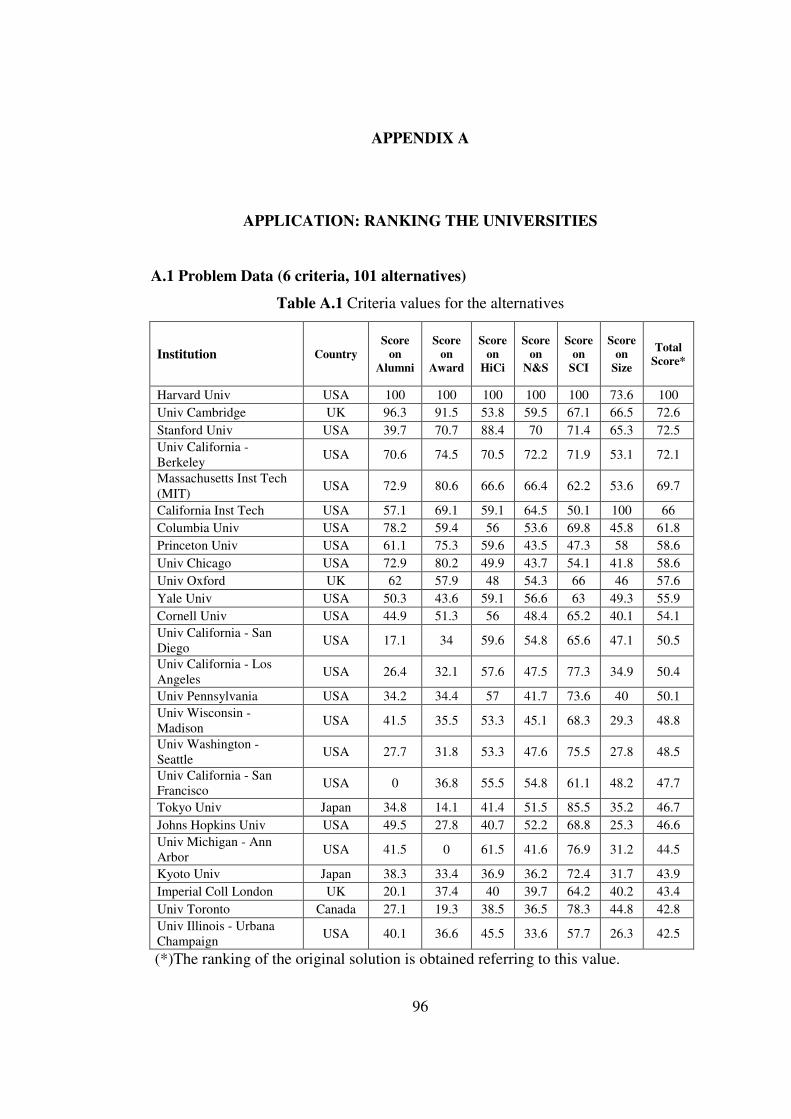
96

APPENDIX A

APPLICATION: RANKING THE UNIVERSITIES

A.1 Problem Data (6 criteria, 101 alternatives)

Table A.1 Criteria values for the alternatives

Institution Country Score

on Alumni

Score on

Award

Score on

HiCi

Score on

N&S

Score on

SCI

Score on

Size

Total Score*

Harvard Univ USA 100 100 100 100 100 73.6 100

Univ Cambridge UK 96.3 91.5 53.8 59.5 67.1 66.5 72.6

Stanford Univ USA 39.7 70.7 88.4 70 71.4 65.3 72.5 Univ California - Berkeley

USA 70.6 74.5 70.5 72.2 71.9 53.1 72.1

Massachusetts Inst Tech (MIT)

USA 72.9 80.6 66.6 66.4 62.2 53.6 69.7

California Inst Tech USA 57.1 69.1 59.1 64.5 50.1 100 66

Columbia Univ USA 78.2 59.4 56 53.6 69.8 45.8 61.8

Princeton Univ USA 61.1 75.3 59.6 43.5 47.3 58 58.6

Univ Chicago USA 72.9 80.2 49.9 43.7 54.1 41.8 58.6

Univ Oxford UK 62 57.9 48 54.3 66 46 57.6

Yale Univ USA 50.3 43.6 59.1 56.6 63 49.3 55.9

Cornell Univ USA 44.9 51.3 56 48.4 65.2 40.1 54.1 Univ California - San Diego

USA 17.1 34 59.6 54.8 65.6 47.1 50.5

Univ California - Los Angeles

USA 26.4 32.1 57.6 47.5 77.3 34.9 50.4

Univ Pennsylvania USA 34.2 34.4 57 41.7 73.6 40 50.1 Univ Wisconsin - Madison

USA 41.5 35.5 53.3 45.1 68.3 29.3 48.8

Univ Washington - Seattle

USA 27.7 31.8 53.3 47.6 75.5 27.8 48.5

Univ California - San Francisco

USA 0 36.8 55.5 54.8 61.1 48.2 47.7

Tokyo Univ Japan 34.8 14.1 41.4 51.5 85.5 35.2 46.7

Johns Hopkins Univ USA 49.5 27.8 40.7 52.2 68.8 25.3 46.6 Univ Michigan - Ann Arbor

USA 41.5 0 61.5 41.6 76.9 31.2 44.5

Kyoto Univ Japan 38.3 33.4 36.9 36.2 72.4 31.7 43.9

Imperial Coll London UK 20.1 37.4 40 39.7 64.2 40.2 43.4

Univ Toronto Canada 27.1 19.3 38.5 36.5 78.3 44.8 42.8 Univ Illinois - Urbana Champaign

USA 40.1 36.6 45.5 33.6 57.7 26.3 42.5

(*)The ranking of the original solution is obtained referring to this value.

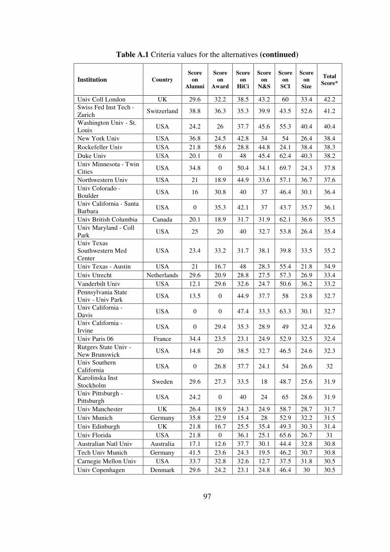
97

Table A.1 Criteria values for the alternatives (continued)

Institution Country Score

on Alumni

Score on

Award

Score on

HiCi

Score on

N&S

Score on

SCI

Score on

Size

Total Score*

Univ Coll London UK 29.6 32.2 38.5 43.2 60 33.4 42.2 Swiss Fed Inst Tech - Zurich

Switzerland 38.8 36.3 35.3 39.9 43.5 52.6 41.2

Washington Univ - St. Louis

USA 24.2 26 37.7 45.6 55.3 40.4 40.4

New York Univ USA 36.8 24.5 42.8 34 54 26.4 38.4

Rockefeller Univ USA 21.8 58.6 28.8 44.8 24.1 38.4 38.3

Duke Univ USA 20.1 0 48 45.4 62.4 40.3 38.2 Univ Minnesota - Twin Cities

USA 34.8 0 50.4 34.1 69.7 24.3 37.8

Northwestern Univ USA 21 18.9 44.9 33.6 57.1 36.7 37.6 Univ Colorado - Boulder

USA 16 30.8 40 37 46.4 30.1 36.4

Univ California - Santa Barbara

USA 0 35.3 42.1 37 43.7 35.7 36.1

Univ British Columbia Canada 20.1 18.9 31.7 31.9 62.1 36.6 35.5 Univ Maryland - Coll Park

USA 25 20 40 32.7 53.8 26.4 35.4

Univ Texas Southwestern Med Center

USA 23.4 33.2 31.7 38.1 39.8 33.5 35.2

Univ Texas - Austin USA 21 16.7 48 28.3 55.4 21.8 34.9

Univ Utrecht Netherlands 29.6 20.9 28.8 27.5 57.3 26.9 33.4

Vanderbilt Univ USA 12.1 29.6 32.6 24.7 50.6 36.2 33.2 Pennsylvania State Univ - Univ Park

USA 13.5 0 44.9 37.7 58 23.8 32.7

Univ California - Davis

USA 0 0 47.4 33.3 63.3 30.1 32.7

Univ California - Irvine

USA 0 29.4 35.3 28.9 49 32.4 32.6

Univ Paris 06 France 34.4 23.5 23.1 24.9 52.9 32.5 32.4 Rutgers State Univ - New Brunswick

USA 14.8 20 38.5 32.7 46.5 24.6 32.3

Univ Southern California

USA 0 26.8 37.7 24.1 54 26.6 32

Karolinska Inst Stockholm

Sweden 29.6 27.3 33.5 18 48.7 25.6 31.9

Univ Pittsburgh - Pittsburgh

USA 24.2 0 40 24 65 28.6 31.9

Univ Manchester UK 26.4 18.9 24.3 24.9 58.7 28.7 31.7

Univ Munich Germany 35.8 22.9 15.4 28 52.9 32.2 31.5

Univ Edinburgh UK 21.8 16.7 25.5 35.4 49.3 30.3 31.4

Univ Florida USA 21.8 0 36.1 25.1 65.6 26.7 31

Australian Natl Univ Australia 17.1 12.6 37.7 30.1 44.4 32.8 30.8

Tech Univ Munich Germany 41.5 23.6 24.3 19.5 46.2 30.7 30.8

Carnegie Mellon Univ USA 33.7 32.8 32.6 12.7 37.5 31.8 30.5

Univ Copenhagen Denmark 29.6 24.2 23.1 24.8 46.4 30 30.5

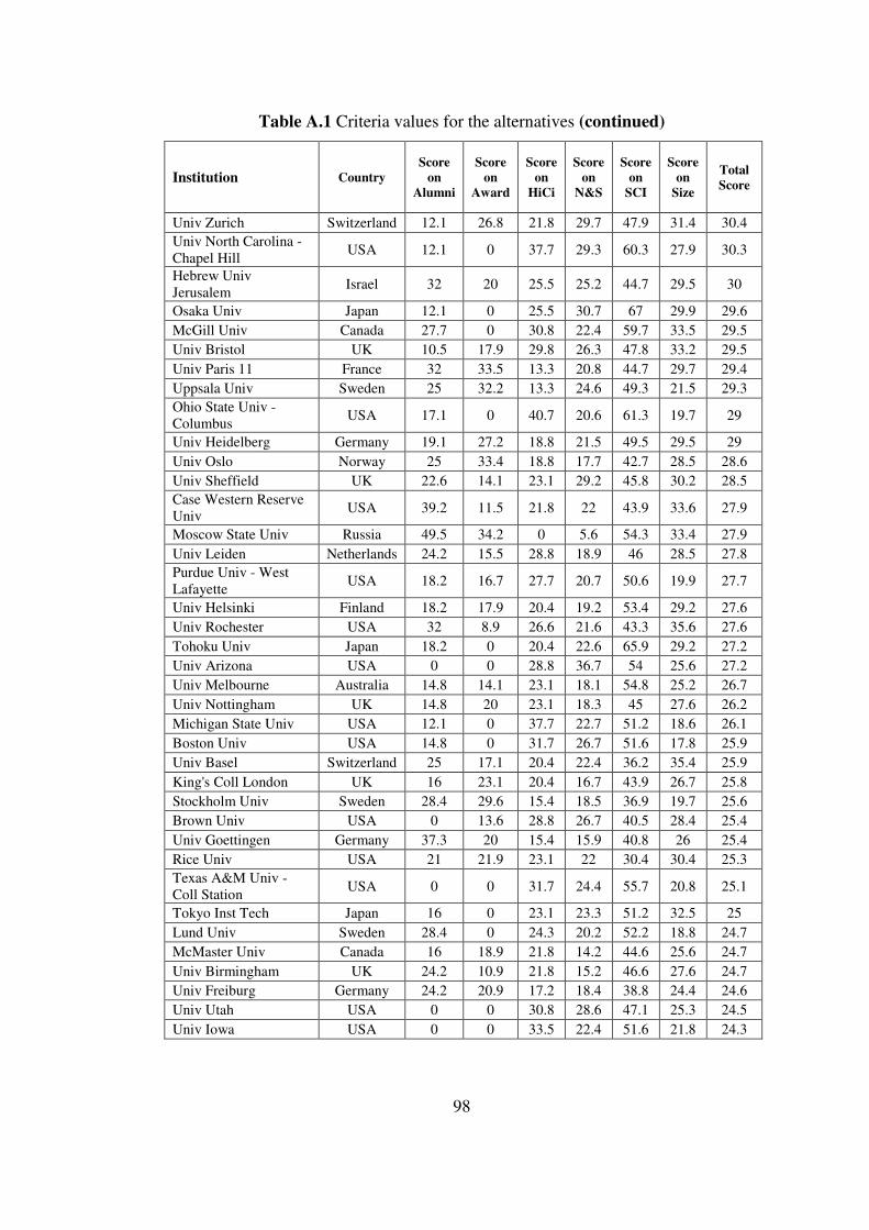
98

Table A.1 Criteria values for the alternatives (continued)

Institution Country Score

on Alumni

Score on

Award

Score on

HiCi

Score on

N&S

Score on

SCI

Score on

Size

Total Score

Univ Zurich Switzerland 12.1 26.8 21.8 29.7 47.9 31.4 30.4 Univ North Carolina - Chapel Hill

USA 12.1 0 37.7 29.3 60.3 27.9 30.3

Hebrew Univ Jerusalem

Israel 32 20 25.5 25.2 44.7 29.5 30

Osaka Univ Japan 12.1 0 25.5 30.7 67 29.9 29.6

McGill Univ Canada 27.7 0 30.8 22.4 59.7 33.5 29.5

Univ Bristol UK 10.5 17.9 29.8 26.3 47.8 33.2 29.5

Univ Paris 11 France 32 33.5 13.3 20.8 44.7 29.7 29.4

Uppsala Univ Sweden 25 32.2 13.3 24.6 49.3 21.5 29.3 Ohio State Univ - Columbus

USA 17.1 0 40.7 20.6 61.3 19.7 29

Univ Heidelberg Germany 19.1 27.2 18.8 21.5 49.5 29.5 29

Univ Oslo Norway 25 33.4 18.8 17.7 42.7 28.5 28.6

Univ Sheffield UK 22.6 14.1 23.1 29.2 45.8 30.2 28.5 Case Western Reserve Univ

USA 39.2 11.5 21.8 22 43.9 33.6 27.9

Moscow State Univ Russia 49.5 34.2 0 5.6 54.3 33.4 27.9

Univ Leiden Netherlands 24.2 15.5 28.8 18.9 46 28.5 27.8 Purdue Univ - West Lafayette

USA 18.2 16.7 27.7 20.7 50.6 19.9 27.7

Univ Helsinki Finland 18.2 17.9 20.4 19.2 53.4 29.2 27.6

Univ Rochester USA 32 8.9 26.6 21.6 43.3 35.6 27.6

Tohoku Univ Japan 18.2 0 20.4 22.6 65.9 29.2 27.2

Univ Arizona USA 0 0 28.8 36.7 54 25.6 27.2

Univ Melbourne Australia 14.8 14.1 23.1 18.1 54.8 25.2 26.7

Univ Nottingham UK 14.8 20 23.1 18.3 45 27.6 26.2

Michigan State Univ USA 12.1 0 37.7 22.7 51.2 18.6 26.1

Boston Univ USA 14.8 0 31.7 26.7 51.6 17.8 25.9

Univ Basel Switzerland 25 17.1 20.4 22.4 36.2 35.4 25.9

King's Coll London UK 16 23.1 20.4 16.7 43.9 26.7 25.8

Stockholm Univ Sweden 28.4 29.6 15.4 18.5 36.9 19.7 25.6

Brown Univ USA 0 13.6 28.8 26.7 40.5 28.4 25.4

Univ Goettingen Germany 37.3 20 15.4 15.9 40.8 26 25.4

Rice Univ USA 21 21.9 23.1 22 30.4 30.4 25.3 Texas A&M Univ - Coll Station

USA 0 0 31.7 24.4 55.7 20.8 25.1

Tokyo Inst Tech Japan 16 0 23.1 23.3 51.2 32.5 25

Lund Univ Sweden 28.4 0 24.3 20.2 52.2 18.8 24.7

McMaster Univ Canada 16 18.9 21.8 14.2 44.6 25.6 24.7

Univ Birmingham UK 24.2 10.9 21.8 15.2 46.6 27.6 24.7

Univ Freiburg Germany 24.2 20.9 17.2 18.4 38.8 24.4 24.6

Univ Utah USA 0 0 30.8 28.6 47.1 25.3 24.5

Univ Iowa USA 0 0 33.5 22.4 51.6 21.8 24.3

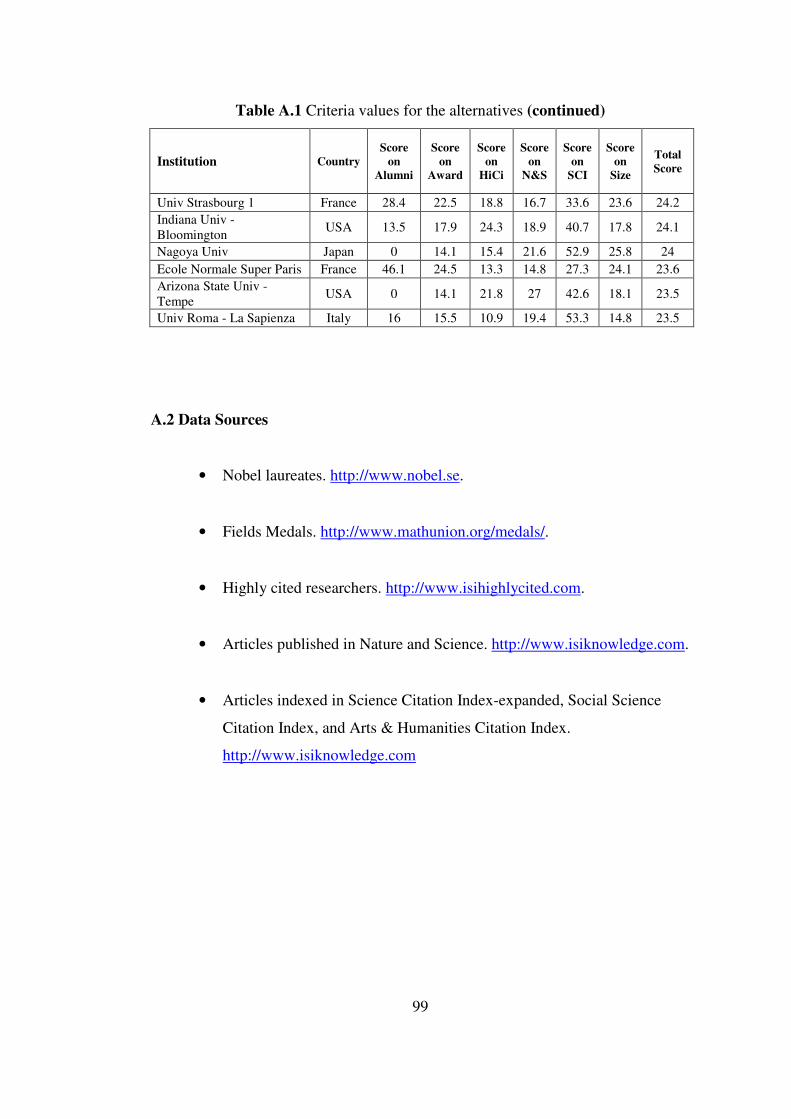
99

Table A.1 Criteria values for the alternatives (continued)

Institution Country Score

on Alumni

Score on

Award

Score on

HiCi

Score on

N&S

Score on

SCI

Score on

Size

Total Score

Univ Strasbourg 1 France 28.4 22.5 18.8 16.7 33.6 23.6 24.2 Indiana Univ - Bloomington

USA 13.5 17.9 24.3 18.9 40.7 17.8 24.1

Nagoya Univ Japan 0 14.1 15.4 21.6 52.9 25.8 24

Ecole Normale Super Paris France 46.1 24.5 13.3 14.8 27.3 24.1 23.6 Arizona State Univ - Tempe

USA 0 14.1 21.8 27 42.6 18.1 23.5

Univ Roma - La Sapienza Italy 16 15.5 10.9 19.4 53.3 14.8 23.5

A.2 Data Sources

• Nobel laureates. http://www.nobel.se.

• Fields Medals. http://www.mathunion.org/medals/.

• Highly cited researchers. http://www.isihighlycited.com.

• Articles published in Nature and Science. http://www.isiknowledge.com.

• Articles indexed in Science Citation Index-expanded, Social Science

Citation Index, and Arts & Humanities Citation Index.

http://www.isiknowledge.com

100

A.3 Rankings for the top 101 universities around the world

Table A.2 Rankings obtained

Methodology Application

Institution Original

Study

Scen. I Original Weights

Scen. II

Matrix Mult.

Scen. III ANP (.5,.5)

Harvard Univ 1 1 1 1

Univ Cambridge 2 5 5 5

Stanford Univ 3 3 3 3

Univ California - Berkeley 4 2 2 2

Massachusetts Inst Tech (MIT) 5 4 4 4

California Inst Tech 6 6 6 6

Columbia Univ 7 7 7 7

Princeton Univ 8 13 11 11

Univ Chicago 8 16 15 15

Univ Oxford 10 10 10 10

Yale Univ 11 8 8 8

Cornell Univ 12 11 12 12

Univ California - San Diego 13 9 9 9

Univ California - Los Angeles 14 14 16 16

Univ Pennsylvania 15 15 14 14

Univ Wisconsin - Madison 16 19 23 20

Univ Washington - Seattle 17 21 24 21

Univ California - San Francisco 18 12 13 13

Tokyo Univ 19 17 18 17

Johns Hopkins Univ 20 24 29 28

Univ Michigan - Ann Arbor 21 18 19 19

Kyoto Univ 22 29 28 29

Imperial Coll London 23 22 20 22

Univ Toronto 24 25 21 24

Univ Illinois - Urbana Champaign 25 31 33 32

Univ Coll London 26 26 27 25

Swiss Fed Inst Tech - Zurich 27 28 25 27

Washington Univ - St. Louis 28 23 22 23

New York Univ 29 34 36 36

Rockefeller Univ 30 41 37 38

Duke Univ 31 20 17 18

Univ Minnesota - Twin Cities 32 33 35 33

Northwestern Univ 33 27 26 26

Univ Colorado - Boulder 34 35 34 35

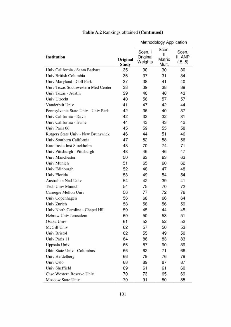
101

Table A.2 Rankings obtained (Continued)

Methodology Application

Institution Original

Study

Scen. I Original Weights

Scen. II

Matrix Mult.

Scen. III ANP (.5,.5)

Univ California - Santa Barbara 35 30 30 30

Univ British Columbia 36 37 31 34

Univ Maryland - Coll Park 37 38 41 40

Univ Texas Southwestern Med Center 38 39 38 39

Univ Texas - Austin 39 40 48 43

Univ Utrecht 40 56 57 57

Vanderbilt Univ 41 47 42 44

Pennsylvania State Univ - Univ Park 42 36 40 37

Univ California - Davis 42 32 32 31

Univ California - Irvine 44 43 43 42

Univ Paris 06 45 59 55 58

Rutgers State Univ - New Brunswick 46 44 51 46

Univ Southern California 47 52 58 56

Karolinska Inst Stockholm 48 70 74 71

Univ Pittsburgh - Pittsburgh 48 46 46 47

Univ Manchester 50 63 63 63

Univ Munich 51 65 60 62

Univ Edinburgh 52 48 47 48

Univ Florida 53 49 54 54

Australian Natl Univ 54 42 39 41

Tech Univ Munich 54 75 70 72

Carnegie Mellon Univ 56 77 72 76

Univ Copenhagen 56 68 66 64

Univ Zurich 58 58 56 59

Univ North Carolina - Chapel Hill 59 45 44 45

Hebrew Univ Jerusalem 60 50 53 51

Osaka Univ 61 53 52 52

McGill Univ 62 57 50 53

Univ Bristol 62 55 49 50

Univ Paris 11 64 86 83 83

Uppsala Univ 65 87 90 89

Ohio State Univ - Columbus 66 62 71 66

Univ Heidelberg 66 79 76 79

Univ Oslo 68 89 87 87

Univ Sheffield 69 61 61 60

Case Western Reserve Univ 70 73 65 69

Moscow State Univ 70 91 80 85

102

Table A.2 Rankings obtained (Continued)

Methodology Application

Institution Original

Study

Scen. I Original Weights

Scen. II

Matrix Mult.

Scen. III ANP (.5,.5)

Univ Leiden 72 60 62 61

Purdue Univ - West Lafayette 73 80 86 82

Univ Helsinki 74 81 78 80

Univ Rochester 74 54 45 49

Tohoku Univ 76 76 73 74

Univ Arizona 76 51 59 55

Univ Melbourne 78 84 85 86

Univ Nottingham 79 85 84 84

Michigan State Univ 80 67 75 70

Boston Univ 81 69 77 73

Univ Basel 81 78 67 75

King's Coll London 83 93 91 93

Stockholm Univ 84 100 100 100

Brown Univ 85 66 68 68

Univ Goettingen 85 97 95 96

Rice Univ 87 82 82 81

Texas A&M Univ - Coll Station 88 72 79 77

Tokyo Inst Tech 89 71 64 67

Lund Univ 90 88 92 91

McMaster Univ 90 95 94 94

Univ Birmingham 90 92 88 90

Univ Freiburg 93 96 96 97

Univ Utah 94 64 69 65

Univ Iowa 95 74 81 78

Univ Strasbourg 1 96 99 98 99

Indiana Univ - Bloomington 97 94 97 95

Nagoya Univ 98 90 89 92

Ecole Normale Super Paris 99 101 101 101

Arizona State Univ - Tempe 100 83 93 88

Univ Roma - La Sapienza 100 98 99 98