Multigrid finite element methods on semi-structured triangular grids for planar elasticity

NUMERICAL LINEAR ALGEBRA WITH APPLICATIONSNumer. Linear Algebra Appl. 2010; 17:473–493Published online 8 December 2009 in Wiley InterScience (www.interscience.wiley.com). DOI: 10.1002/nla.684

Multigrid finite element methods on semi-structured triangulargrids for planar elasticity

F. J. Gaspar∗,†, F. J. Lisbona, J. L. Gracia and C. Rodrigo

Applied Mathematics Department, University of Zaragoza, Zaragoza, Spain

SUMMARY

Multigrid methods for a stencil-based implementation of a finite element method for planar elasticity,using semi-structured triangular grids, are presented. Local Fourier analysis (LFA) is applied to identifythe correct multigrid components. To this end, LFA for multigrid methods on regular triangular gridsis extended to the case of the problem of planar elasticity, although its application to other systems isstraightforward. For the discrete elasticity operator obtained with linear finite elements, different collectivesmoothers, such as three-color smoother and some zebra-type smoothers, are analyzed, and LFA resultsfor these smoothers are shown. The multigrid method is constructed in a block-wise form. In particular,different smoothers and different numbers of pre- and post-smoothing steps are considered in each triangleof the coarsest triangulation of the domain. Some numerical experiments are presented to illustrate theefficiency of this multigrid algorithm. Copyright q 2009 John Wiley & Sons, Ltd.

Received 19 May 2009; Revised 21 October 2009; Accepted 23 October 2009

KEY WORDS: planar elasticity; finite elements; semi-structured grids; geometric multigrid; local Fourieranalysis

1. INTRODUCTION

Multigrid methods [1–4] are highly efficient numerical techniques for solving the algebraic linearequation systems arising from the discretization of partial differential equations. In geometricmultigrid, a hierarchy of grids must be proposed. For an irregular domain, it is very commonto apply regular refinement to an unstructured input grid; in this way, a hierarchy of globallyunstructured grids is generated that is suitable for use with geometric multigrid. So, we areinterested in the framework of hierarchical hybrid grids (HHG), which was presented in [5]. Thecoarsest mesh is assumed so that it fits the geometry of the domain. Once this coarse triangulation

∗Correspondence to: F. J. Gaspar, Applied Mathematics Department, University of Zaragoza, Zaragoza, Spain.†E-mail: [email protected]

Contract/grant sponsor: FEDER/MCYT; contract/grant number: MTM2007-63204Contract/grant sponsor: DGA

Copyright q 2009 John Wiley & Sons, Ltd.

474 F. J. GASPAR ET AL.

is given, each triangle is divided into four congruent triangles, connecting the midpoints of theiredges, and so forth until the mesh has the desired fine scale to approximate the solution of theproblem. In this way, a nested hierarchy of grids is obtained.

The hierarchical hybrid grids framework provides certain advantages in the implementation ofa geometric multigrid algorithm. Transfer operations between grids can be defined geometrically,allowing a straightforward implementation of the multigrid algorithm. Moreover, HHG exploitsthe regularity of grids, in such a way that it is not necessary to assemble the whole stiffness matrix,and therefore the multigrid method can be implemented using stencil-based operations, drasticallyreducing the memory required. Note that one stencil suffices to represent the discrete operator atnodes inside a triangle of the coarsest grid.

In order to choose suitable components for a multigrid method, Local Fourier analysis (LFA)is used. This analysis is particularly valuable for systems of PDEs, since it is often much moredifficult to identify the correct multigrid components than for a scalar problem. LFA is mainlybased on the Fourier transform and was introduced by Brandt in [6]. A good introduction can befound in the books by Trottenberg et al. [3] and Wienands and Joppich [7]. This technique hasbeen widely used for systems of PDEs in the framework of discretizations on rectangular grids[8–11]; even for the elasticity problem an alternative approach to Fourier analysis was developedin [12]. Recently a generalization of LFA to triangular grids has been proposed in [13] for ascalar problem, and in [14] it has been extended using a three-coarsening strategy. The key tocarrying out this generalization is to write the Fourier transform in new coordinate systems, both inspace and in frequency variables, associated with reciprocal bases fitting the structure of the grid.In order to extend LFA to the case of the planar elasticity system, an expression of the Fouriertransform for vector functions must be considered. To study the efficiency of multigrid methodsin the framework of HHG, LFA is applied to each input triangle in such a way that the globalbehavior of the method will depend on the quality of the chosen local components.

In the context of computational solid mechanics, multigrid methods have been applied to linearelasticity problems by some authors. In 1990, Parsons investigated the performance of a multigridalgorithm by applying it to two-dimensional problems in [15] and to some three-dimensionalproblems of practical interest in [16]. Besides, in [17], adaptive local grid refinement and multigridon parallel computers were combined to solve linear elasticity problems, studying in detail theproblem of dynamic load balancing. Some algebraic multigrid (AMG) approaches have also beenapplied to this kind of problems. In [18], Ruge presented results of the performance of AMGfor different types of discretizations of a model plane elasticity problem. In [19], for 3D elas-ticity problem discretized by quadratic elements, an algebraic convergence theory for two levelmethods was developed using linear elements in the coarse level. Griebel et al. [20] generalizedthe classical AMG approach for scalar problems to systems of PDEs in a natural block-wisefashion, and Kraus [21] has recently performed an AMG based on computational molecules forself-adjoint and elliptic problems arising from finite element discretization of the linear elasticitymodel, providing efficient solutions of problems with discontinuous coefficients, e.g. for compositematerials.

The organization of the paper is as follows: In Section 2, we describe the discrete operator ina stencil-based form, and a procedure to compute it using a canonical stencil associated with areference hexagon is given. Moreover, the components of the multigrid algorithm are also presented.In Section 3, some LFA results are shown in order to choose the components of the multigridalgorithm which are more suitable for different grid geometries, and finally in Section 4, twonumerical experiments illustrate the good behavior of the method.

Copyright q 2009 John Wiley & Sons, Ltd. Numer. Linear Algebra Appl. 2010; 17:473–493DOI: 10.1002/nla

MULTIGRID FEM ON SEMI-STRUCTURED TRIANGULAR GRIDS 475

2. DISCRETIZATION OF PLANAR ELASTICITY

2.1. Formulation of the problem

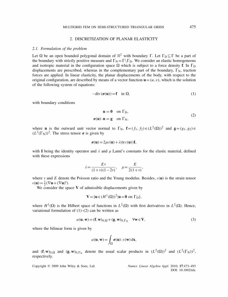
Let � be an open bounded polygonal domain of R2 with boundary �. Let �D⊆� be a part ofthe boundary with strictly positive measure and �N=�\�D. We consider an elastic homogeneousand isotropic material in the configuration space � which is subject to a force density f. In �Ddisplacements are prescribed, whereas in the complementary part of the boundary, �N, tractionforces are applied. In linear elasticity, the planar displacements of the body, with respect to theoriginal configuration, are described by means of a vector function u=(u,v), which is the solutionof the following system of equations:

−div(r(u))= f in �, (1)

with boundary conditions

u = 0 on �D,

r(u) ·n = g on �N,(2)

where n is the outward unit vector normal to �N, f=( f1, f2)∈(L2(�))2 and g=(g1,g2)∈(L2(�N))2. The stress tensor r is given by

r(u)=2�ε(u)+�(trε(u))I,

with I being the identity operator and � and � Lame’s constants for the elastic material, definedwith these expressions

�= E�

(1+�)(1−2�), �= E

2(1+�),

where � and E denote the Poisson ratio and the Young modulus. Besides, ε(u) is the strain tensorε(u)= 1

2 (∇u+(∇u)t).We consider the space V of admissible displacements given by

V={u∈(H1(�))2|u=0 on �D},where H1(�) is the Hilbert space of functions in L2(�) with first derivatives in L2(�). Hence,variational formulation of (1)–(2) can be written as

a(u,w)=(f,w)0,�+(g,w)0,�N ∀w∈V, (3)

where the bilinear form is given by

a(u,w)=∫

�r(u) :ε(w)dx,

and (f,w)0,� and (g,w)0,�N denote the usual scalar products in (L2(�))2 and (L2(�N))2,respectively.



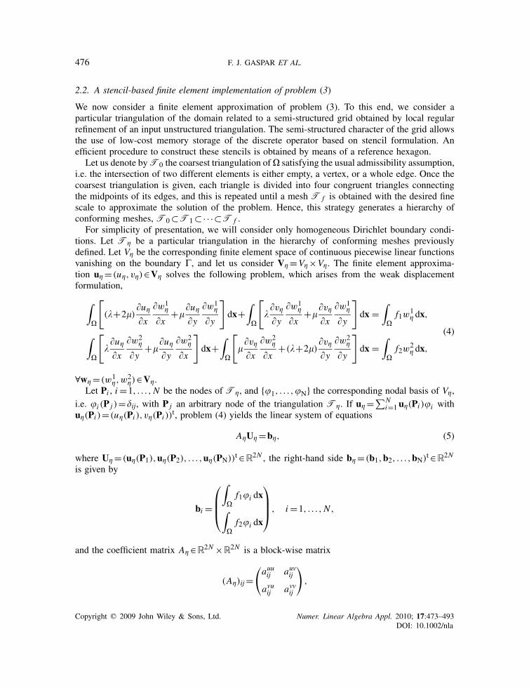
2.2. A stencil-based finite element implementation of problem (3)

We now consider a finite element approximation of problem (3). To this end, we consider aparticular triangulation of the domain related to a semi-structured grid obtained by local regularrefinement of an input unstructured triangulation. The semi-structured character of the grid allowsthe use of low-cost memory storage of the discrete operator based on stencil formulation. Anefficient procedure to construct these stencils is obtained by means of a reference hexagon.

Let us denote byT0 the coarsest triangulation of� satisfying the usual admissibility assumption,i.e. the intersection of two different elements is either empty, a vertex, or a whole edge. Once thecoarsest triangulation is given, each triangle is divided into four congruent triangles connectingthe midpoints of its edges, and this is repeated until a mesh T f is obtained with the desired finescale to approximate the solution of the problem. Hence, this strategy generates a hierarchy ofconforming meshes, T0⊂T1⊂·· ·⊂T f .

For simplicity of presentation, we will consider only homogeneous Dirichlet boundary condi-tions. Let T� be a particular triangulation in the hierarchy of conforming meshes previouslydefined. Let V� be the corresponding finite element space of continuous piecewise linear functionsvanishing on the boundary �, and let us consider V� =V�×V�. The finite element approxima-tion u� =(u�,v�)∈V� solves the following problem, which arises from the weak displacementformulation,

∫�

[(�+2�)

�u�

�x

�w1�

�x+�

�u�

�y

�w1�

�y

]dx+

∫�

[��v�

�y

�w1�

�x+�

�v�

�x

�w1�

�y

]dx =

∫�f1w

1� dx,

∫�

[��u�

�x

�w2�

�y+�

�u�

�y

�w2�

�x

]dx+

∫�

[�

�v�

�x

�w2�

�x+(�+2�)

�v�

�y

�w2�

�y

]dx =

∫�f2w

2� dx,

(4)

∀w� =(w1�,w

2�)∈V�.

Let Pi , i=1, . . . ,N be the nodes of T�, and {�1, . . . ,�N} the corresponding nodal basis of V�,i.e. �i (P j )=�ij, with P j an arbitrary node of the triangulation T�. If u� =∑N

i=1u�(Pi )�i withu�(Pi )=(u�(Pi ),v�(Pi ))

t, problem (4) yields the linear system of equations

A�U� =b�, (5)

where U� =(u�(P1),u�(P2), . . . ,u�(PN))t∈R2N , the right-hand side b� =(b1,b2, . . . ,bN)t∈R2N

is given by

bi =

⎛⎜⎜⎝∫

�f1�i dx∫

�f2�i dx

⎞⎟⎟⎠ , i=1, . . . ,N ,

and the coefficient matrix A� ∈R2N ×R2N is a block-wise matrix

(A�)ij=(auuij auvij

avuij avvij

),



whose (2×2)-blocks are given by

auuij =∫

�

[(�+2�)

�� j

�x��i

�x+�

�� j

�y��i

�y

]dx,

auvij =∫

�

[�� j

�y��i

�x+�

�� j

�x��i

�y

]dx,

avuij =∫

�

[�� j

�x��i

�y+�

�� j

�y��i

�x

]dx,

avvij =∫

�

[�

�� j

�x��i

�x+(�+2�)

�� j

�y��i

�y

]dx.

We distinguish among interior nodes of a triangle of the coarsest grid, vertices of T0 and nodeslying on one edge of triangles onT0, see Figure 1. Depending on the location of a node in the grid,the way in which the discrete operator L� is given is different. As we deal with a semi-structuredgrid, the discrete operator can be defined using a stencil form for interior points to each coarsetriangle and a different stencil form for nodes lying on the edges of T0. However, in order todescribe L� in the nodes on T0, it is necessary to construct the stiffness matrix on the coarsestgrid, which will be scaled depending on the refinement level we are working with.

For instance, with the purpose of constructing the stencil associated with an interior point of atriangle T of the coarsest grid, we are going to define the regular grid arising inside this triangle.To this end, we consider a unitary basis of R2, {e′

1,e′2}, fitting the geometry of the triangle, as we

can see in Figure 2. Thus, we can define the grid for the refinement level � in the following way:

GT,� ={x′ =(x ′1, x

′2)|x ′

i =ki hi , i=1,2, k1=0, . . . ,2�, k2=0, . . . ,k1},

Figure 1. Different kinds of nodes on a triangle of the coarsest grid.



e

e

Figure 2. New basis in R2 fitting the geometry of a triangle of the coarsest grid, and local numeration.

Figure 3. Reference hexagon and corresponding affine transformation FH .

where h=(h1,h2) is the grid spacing in triangle T, associated with the refinement level �, so thatthe grid GT,� can also be denoted by Gh . Hence, a local numeration in each one of the trianglesof the coarsest grid can be fixed according to the definition of the spatial basis. For a refinementlevel �, a local numeration with double index (k1,k2), k1=0, . . . ,2�, k2=0, . . . ,k1, is used in sucha way that the indexes of the vertices of the triangle are (0,0), (2�,0), (2�,2�), as we can alsoobserve in Figure 2 for �=2.

2.2.1. Stencil construction. Each interior node to a triangle of the grid T0 is the center of ahexagon H , consisting of six congruent triangles, which is the support of the correspondingnodal basis function. Using local numeration, we denote by xn,m the central point, and byxn+1,m,xn−1,m,xn,m+1,xn,m−1,xn+1,m+1,xn−1,m−1, the vertices of this hexagon (Figure 3). Notethat in this situation we can use the step size of the grid h=(h1,h2) as discretization parameter. Inthe system of Equations (5), we have two equations associated with a fixed node xn,m , which are:

∑j∈I

suuj uh(xn+�1,m+�2)+∑j∈I

suvj vh(xn+�1,m+�2) =∫H

f1�n,m dx,

∑j∈I

svuj uh(xn+�1,m+�2)+∑j∈I

svvj vh(xn+�1,m+�2) =∫H

f2�n,m dx,(6)



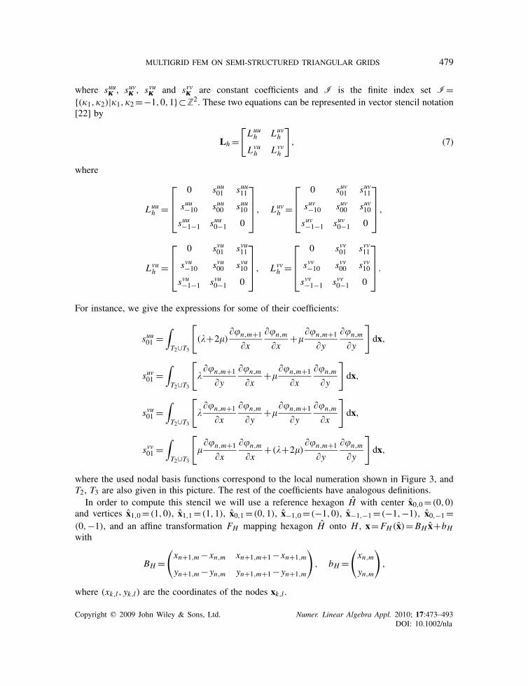
where suuj , suvj , svuj and svvj are constant coefficients and I is the finite index set I={(�1,�2)|�1,�2=−1,0,1}⊂Z2. These two equations can be represented in vector stencil notation[22] by

Lh =[Luuh Luv

h

Lvuh Lvv

h

], (7)

where

Luuh =

⎡⎢⎢⎣

0 suu01 suu11

suu−10 suu00 suu10

suu−1−1 suu0−1 0

⎤⎥⎥⎦ , Luv

h =

⎡⎢⎢⎣

0 suv01 suv11

suv−10 suv00 suv10

suv−1−1 suv0−1 0

⎤⎥⎥⎦ ,

Lvuh =

⎡⎢⎢⎣

0 svu01 svu11

svu−10 svu00 svu10

svu−1−1 svu0−1 0

⎤⎥⎥⎦ , Lvv

h =

⎡⎢⎢⎣

0 svv01 svv11

svv−10 svv00 svv10

svv−1−1 svv0−1 0

⎤⎥⎥⎦ .

For instance, we give the expressions for some of their coefficients:

suu01 =∫T2∪T3

[(�+2�)

��n,m+1

�x��n,m

�x+�

��n,m+1

�y��n,m

�y

]dx,

suv01 =∫T2∪T3

[��n,m+1

�y��n,m

�x+�

��n,m+1

�x��n,m

�y

]dx,

svu01 =∫T2∪T3

[��n,m+1

�x��n,m

�y+�

��n,m+1

�y��n,m

�x

]dx,

svv01 =∫T2∪T3

[�

��n,m+1

�x��n,m

�x+(�+2�)

��n,m+1

�y��n,m

�y

]dx,

where the used nodal basis functions correspond to the local numeration shown in Figure 3, andT2, T3 are also given in this picture. The rest of the coefficients have analogous definitions.

In order to compute this stencil we will use a reference hexagon H with center x0,0=(0,0)and vertices x1,0=(1,0), x1,1=(1,1), x0,1=(0,1), x−1,0=(−1,0), x−1,−1=(−1,−1), x0,−1=(0,−1), and an affine transformation FH mapping hexagon H onto H , x=FH (x)= BH x+bHwith

BH =(xn+1,m−xn,m xn+1,m+1−xn+1,m

yn+1,m− yn,m yn+1,m+1− yn+1,m

), bH =

(xn,m

yn,m

),

where (xk,l , yk,l) are the coordinates of the nodes xk,l .



With these definitions, we can translate the degrees of freedom and basis functions on thereference hexagon (denoted here by �) to degrees of freedom and basis functions on the concretehexagon H . In particular, we have

�k,l =�k,l ◦FH , ∇�k,l = BtH∇�k,l ◦FH .

By applying the change of variable associated with the affine mapping, and defining the matrixB−1H as

B−1H =

(bH11 bH12

bH21 bH22

),

the stencils defined before can be written in terms of certain reference stencils in the followingway:

Luuh = |det BH |(((�+2�)(bH11)

2+�(bH12)2)Lxx+(�(bH22)

2+(�+2�)(bH21)2)Lyy

+((�+2�)bH11bH21+�bH22b

H12)(Lxy+Lyx)),

Luvh = |det BH |((�+�)bH11b

H12Lxx+(�+�)bH22b

H21Lyy+(�bH12b

H21+�bH22b

H11)Lxy

+(�bH22bH11+�bH21b

H12)Lyx),

Lvuh = |det BH |((�+�)bH11b

H12Lxx+(�+�)bH22b

H21Lyy+(�bH22b

H11+�bH21b

H12)Lxy

+(�bH12bH21+�bH22b

H11)Lyx),

Lvvh = |det BH |(((�+2�)(bH12)

2+�(bH11)2)Lxx+(�(bH21)

2+(�+2�)(bH22)2)Lyy

+((�+2�)bH22bH12+�bH11b

H21)(Lxy+Lyx)),

where

Lxx=⎡⎢⎣

0 0 0

−1 2 −1

0 0 0

⎤⎥⎦ , Lxy= Lyx= 1

2

⎡⎢⎣

0 1 −1

1 −2 1

−1 1 0

⎤⎥⎦ , Lyy=

⎡⎢⎣0 −1 0

0 2 0

0 −1 0

⎤⎥⎦ ,

are the stencils associated with operators −�xx,−�xy,−�yx and −�yy, respectively, in the referencehexagon.

Finally, we normalize equations in (6) with the factor |det BH |, and then the right–hand side isan approximation of f(xn,m).

With obvious modifications of the previous process, it is possible to construct the stencilassociated with the nodes located at the edges in T0. Finally, as the number of neighbors of thenodes which are vertices of T0 is not fixed, the corresponding equations cannot be represented instencil form. For this reason, it is necessary to assemble and normalize the matrix for the coarsestgrid with the integral of �i over its support. Therefore, the intrinsic operations associated withthese nodes in the multigrid algorithm will be performed by appropriately using the correspondingrows of the assembled matrix on the coarsest grid. In the same way, in any refinement level, the



equations corresponding to these nodes can be obtained by scaling the corresponding rows of theassembled matrix on the coarsest grid.

2.3. Multigrid solver on semi-structured grids

As is well known, the construction of an efficient multigrid method is strongly dependent on thechoice of its components. The main components are the smoother Sh , inter-grid transfer operators:restriction R2h

h and prolongation Ph2h and the coarse-grid operator L2h . These components have to

be selected so that they efficiently interplay with each other. Especially, the choice of a suitablesmoother is an important feature for the design of an efficient geometric multigrid method.

We use a block-wise multigrid algorithm, where each one of the triangles of the coarsest gridis treated as a different block with regard to the smoothing process. In the relaxation method, firstwe loop over unknowns located at the vertices of the coarsest grid, and then we loop over the restof the unknowns using the corresponding smoother for each triangular block. Moreover, a properboundary treatment is included, which consists of an extra relaxation near the internal and externalboundaries of each coarsest triangle. This block-wise strategy is suitable because of the possibilityof choosing different smoothers for triangles that have different geometries, thus resulting in animprovement of the characteristics of our algorithm.

In this paper, a linear interpolation has been chosen, the restriction operator has been taken as itsadjoint, and the discrete operator corresponding to each mesh results from the direct discretizationof the problem. Moreover, collective three-color smoother and some collective line-wise smoothersare proposed as relaxing methods. These smoothers appear as a natural extension to triangulargrids of some smoothers widely used on rectangular grids, as red-black Gauss–Seidel and line-wiserelaxations of zebra type.

To apply three-color smoother, the grid associated with a fixed refinement level of a triangle ofthe coarsest triangulation, Gh , is split into three disjoint sets

Gih ={x′ =(x ′

1, x′2)∈Gh |x ′

j =k j h j , j =1,2,k1+k2= i(mod3)}, i=0,1,2,

with each set having a different color (red, black or green), as shown in Figure 4(a), so that theunknowns of the same color have no direct connection with each other. Note that, in general, thechoice of the disjoint subsets Gi

h depends on the nonzero pattern of the particular stencil underconsideration.

Considering a damping parameter, collective three-color-Jacobi smoother (which is identicalto collective three-color -Gauss–Seidel smoother for seven-point stencils on triangular grids)is defined as three partial sweeps of a collective –Jacobi smoother, each of one updating theunknowns of the same color, for example in the order G0

h , G1h and G2

h . Note that all the unknownsassociated with each point are simultaneously updated, and therefore for the considered problema linear 2×2-system of equations, corresponding to the two displacement components, have tobe solved. In each partial relaxation step, only the grid points of Gi

h are processed, whereas theremaining points are not treated, that is,

Sih()vh(x)={[(Ih−D−1

h Lh)vh](x), x∈Gih,

vh(x), x∈Gh\Gih,

where Dh is the corresponding block-diagonal part of the discrete operator Lh . Therefore, thecomplete three-color smoothing operator is given by the product of these three partial step operators,Sh()=S2h()S1h()S0h().



(a) (b)

Figure 4. (a) Three-color smoother. (b) Zebra-red smoother: approximations at points marked by 1 areupdated in the first half-step of the relaxation, those marked by 2 in the second.

Table I. Characterization of subgrids Gevenh and Godd

h for thedifferent zebra smoothers.

Relaxation Gevenh Godd

h

Zebra-red k2 even k2 oddZebra-black k1 even k1 oddZebra-green k1+k2 even k1+k2 odd

Line-wise smoothers considered in this paper are of zebra type. In rectangular grids, zebra-typerelaxation is the line analog to point-wise red-black smoothing in the sense that it again consists oftwo half-steps. In the first half-step even lines are processed, whereas odd lines are relaxed in thesecond step, in which the updated approximations on the even lines are used. For triangular grids,three different zebra smoothers can be defined on a triangle. We will denote them as zebra-red,zebra-black and zebra-green smoothers, since they correspond to each of the vertices of the trianglewhich can be associated with these colors. In Figure 4(b) the zebra-type smoother correspondingto the red vertex is shown.

In order to apply these smoothers, a splitting of the grid Gh into two different subsets Gevenh

and Goddh is necessary. For each of the zebra smoothers these subgrids are defined in a different

way, and the corresponding distinction between them is specified in Table I. Thus, these threesmoothers, SzRh , SzBh , and SzGh are defined by the product of two partial step operators:

SzRh = SzR−oddh SzR−even

h ,

SzBh = SzB−oddh SzB−even

h ,

SzGh = SzG−oddh SzG−even

h ,

where these partial step operators only relax the grid points of the corresponding subgrid, whereasthe remaining points are not treated. These smoothers are preferred to the lexicographic line-wise



Gauss–Seidel because in spite of having the same computational cost, smoothing factors corre-sponding to zebra smoothers are better than those of lexicographic line-wise relaxations, and theyare more suitable for parallel implementation.

3. FOURIER ANALYSIS RESULTS

LFA is a tool used for the design of efficient multigrid methods on regular structured grids.Recently, a generalization to triangular grids—which is based on an expression of the Fouriertransform in new coordinate systems in space and frequency variables—has been proposed in [13].The ideas developed in that paper can be extended to systems of equations similarly as in cartesiangrids, see [1, 3, 7].

In the context of discretizations on semi-structured grids, particularly in the case of the hierar-chical triangular meshes considered in this paper, an LFA is used to predict the behavior of themultigrid method on each triangular block of the coarsest grid. The quality of the general algorithmwill depend on the local results obtained for each coarse triangle.

In Fourier smoothing analysis, the influence of a smoothing operator on the high-frequencyerror components is investigated. To get more insight into the structure of a multigrid algorithm, itis useful to perform a two-grid analysis [3] in order to investigate the interplay between relaxationand coarse-grid correction, which is crucial for an efficient multigrid method.

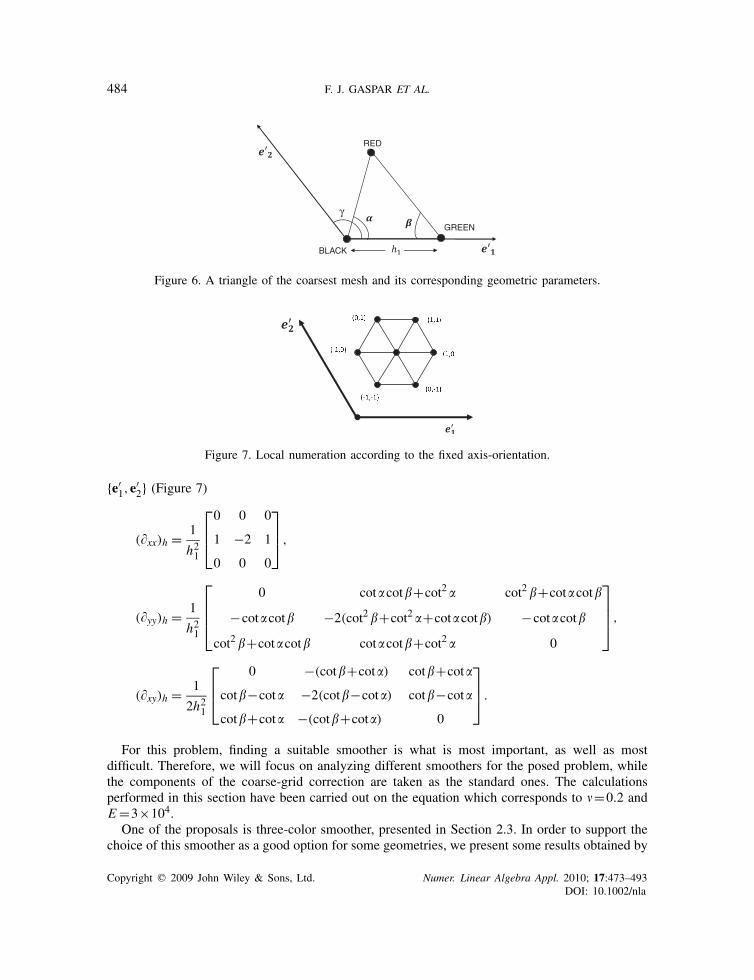
For elasticity problem it is fulfilled that the Fourier symbols of the discrete operators asso-ciated with two grids, one obtained by rotating the other by angle (Figure 5), are similar,that is, they have the same eigenvalues. Therefore, it is possible to restrict the analysis to trian-gles that sit on the x-axis of the Cartesian coordinate system. So, in this section we applyLFA to a discretization of the elasticity operator by linear finite elements on a regular trian-gulation of a general triangle oriented as established before, in order to investigate how thegrid-geometry has influence on the convergence properties of multigrid methods. We consider twoangles of the coarsest triangle, denoted by � and �, and the size of the side between them h1(Figure 6), and we will study the results obtained with LFA varying the values of these geometricparameters.

With this purpose, we formulate the stencil for each one of the involved discrete scalar oper-ators in terms of these parameters, according to the axis-orientation considered in this paper

Figure 5. Rotation by angle of certain hexagon H .



RED

GREEN

BLACK

Figure 6. A triangle of the coarsest mesh and its corresponding geometric parameters.

Figure 7. Local numeration according to the fixed axis-orientation.

{e′1,e

′2} (Figure 7)

(�xx)h = 1

h21

⎡⎢⎣0 0 0

1 −2 1

0 0 0

⎤⎥⎦ ,

(�yy)h = 1

h21

⎡⎢⎢⎣

0 cot�cot�+cot2 � cot2�+cot�cot�

−cot�cot� −2(cot2�+cot2 �+cot�cot�) −cot�cot�

cot2�+cot�cot� cot�cot�+cot2 � 0

⎤⎥⎥⎦ ,

(�xy)h = 1

2h21

⎡⎢⎣

0 −(cot�+cot�) cot�+cot�

cot�−cot� −2(cot�−cot�) cot�−cot�

cot�+cot� −(cot�+cot�) 0

⎤⎥⎦ .

For this problem, finding a suitable smoother is what is most important, as well as mostdifficult. Therefore, we will focus on analyzing different smoothers for the posed problem, whilethe components of the coarse-grid correction are taken as the standard ones. The calculationsperformed in this section have been carried out on the equation which corresponds to �=0.2 andE=3×104.One of the proposals is three-color smoother, presented in Section 2.3. In order to support the

choice of this smoother as a good option for some geometries, we present some results obtained by



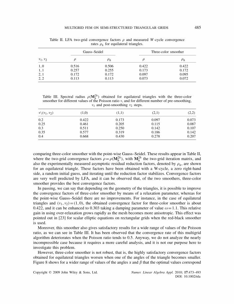
Table II. LFA two-grid convergence factors and measured W -cycle convergencerates h for equilateral triangles.

Gauss–Seidel Three-color smoother

�1,�2 h h

1,0 0.516 0.506 0.422 0.4221,1 0.257 0.255 0.173 0.1722,1 0.172 0.172 0.097 0.0952,2 0.113 0.113 0.073 0.072

Table III. Spectral radius (M2hh ) obtained for equilateral triangles with the three-color

smoother for different values of the Poisson ratio �, and for different number of pre-smoothing,�1 and post-smoothing �2 steps.

�\(�1,�2) (1,0) (1,1) (2,1) (2,2)

0.2 0.422 0.173 0.097 0.0730.25 0.461 0.205 0.115 0.0870.3 0.511 0.250 0.142 0.1070.35 0.577 0.319 0.186 0.1420.4 0.668 0.430 0.278 0.207

comparing three-color smoother with the point-wise Gauss–Seidel. These results appear in Table II,where the two-grid convergence factors = (M2h

h ), with M2hh the two-grid iteration matrix, and

also the experimentally measured asymptotic residual reduction factors, denoted by h , are shownfor an equilateral triangle. These factors have been obtained with a W-cycle, a zero right-handside, a random initial guess, and iterating until the reduction factor stabilizes. Convergence factorsare very well predicted by LFA, and it can be observed that, of the two smoothers, three-colorsmoother provides the best convergence factors.

In passing, we can say that depending on the geometry of the triangles, it is possible to improvethe convergence factors of three-color smoother by means of a relaxation parameter, whereas forthe point-wise Gauss–Seidel there are no improvements. For instance, in the case of equilateraltriangles and (�1,�2)=(1,0), the obtained convergence factor for three-color smoother is about0.422, and it can be enhanced to 0.303 taking a damping parameter of value =1.1. This relativegain in using over-relaxation grows rapidly as the mesh becomes more anisotropic. This effect waspointed out in [23] for scalar elliptic equations on rectangular grids when the red-black smootheris used.

Moreover, this smoother also gives satisfactory results for a wide range of values of the Poissonratio, as we can see in Table III. It has been observed that the convergence rate of this multigridalgorithm deteriorates when the Poisson ratio tends to 0.5. Anyway, we do not analyze the nearlyincompressible case because it requires a more careful analysis, and it is not our purpose here toinvestigate this problem.

However, three-color smoother is not robust, that is, the highly satisfactory convergence factorsobtained for equilateral triangles worsen when one of the angles of the triangle becomes smaller.Figure 8 shows for a wider range of values of the angles � and � that the optimal values correspond



0 10

20 30

40 50

60 70

80 90 0

10 20

30 40

50 60

70 80

90

0.4 0.5 0.6 0.7 0.8 0.9

1

0.80.70.60.5

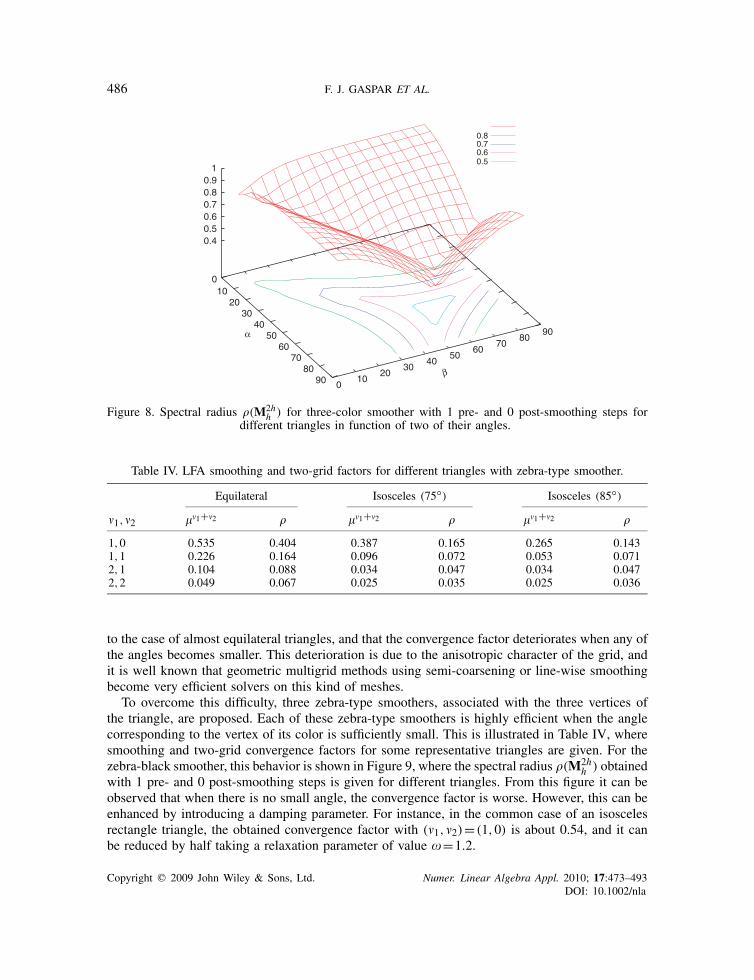
Figure 8. Spectral radius (M2hh ) for three-color smoother with 1 pre- and 0 post-smoothing steps for

different triangles in function of two of their angles.

Table IV. LFA smoothing and two-grid factors for different triangles with zebra-type smoother.

Equilateral Isosceles (75◦) Isosceles (85◦)

�1,�2 ��1+�2 ��1+�2 ��1+�2

1,0 0.535 0.404 0.387 0.165 0.265 0.1431,1 0.226 0.164 0.096 0.072 0.053 0.0712,1 0.104 0.088 0.034 0.047 0.034 0.0472,2 0.049 0.067 0.025 0.035 0.025 0.036

to the case of almost equilateral triangles, and that the convergence factor deteriorates when any ofthe angles becomes smaller. This deterioration is due to the anisotropic character of the grid, andit is well known that geometric multigrid methods using semi-coarsening or line-wise smoothingbecome very efficient solvers on this kind of meshes.

To overcome this difficulty, three zebra-type smoothers, associated with the three vertices ofthe triangle, are proposed. Each of these zebra-type smoothers is highly efficient when the anglecorresponding to the vertex of its color is sufficiently small. This is illustrated in Table IV, wheresmoothing and two-grid convergence factors for some representative triangles are given. For thezebra-black smoother, this behavior is shown in Figure 9, where the spectral radius (M2h

h ) obtainedwith 1 pre- and 0 post-smoothing steps is given for different triangles. From this figure it can beobserved that when there is no small angle, the convergence factor is worse. However, this can beenhanced by introducing a damping parameter. For instance, in the common case of an isoscelesrectangle triangle, the obtained convergence factor with (�1,�2)=(1,0) is about 0.54, and it canbe reduced by half taking a relaxation parameter of value =1.2.



0.1

0.4 0.3 0.2

0.5 0.6 0.7 0.8 0.9

1

0 10 20 30 40 50 60 70 80 90 0 10

20 30 40

50 60 70 80 90

0.80.70.60.5

Figure 9. Spectral radius (M2hh ) for the zebra-black smoother with 1 pre- and 0 post-smoothing steps

for different triangles in function of two of their angles.

Table V. Spectral radius (M2hh ) obtained for an isosceles triangle, with common angle 85◦, with

zebra-type smoother for different values of the Poisson ratio �, and for different number of pre-smoothing�1 and post-smoothing �2 steps.

�\(�1,�2) (1,0) (1,1) (2,1) (2,2)

0.2 0.143 0.071 0.048 0.0360.25 0.168 0.086 0.059 0.0450.3 0.203 0.109 0.076 0.0580.35 0.251 0.146 0.104 0.0820.4 0.325 0.209 0.158 0.127

Analogously to the case of three-color smoother, results obtained with these smoothers varyingthe Poisson ratio � are also good as we can see in Table V. Convergence factors predicted by LFAare shown for an isosceles triangle with common angle 85◦. On the other hand, for this kind ofsmoothers the introduction of a relaxation parameter does not essentially improve the convergencefactors when the corresponding angle is small, that is, when the smoother is really efficient.

From the practical point of view, LFA can be used to choose a suitable smoother and a numberof pre- and post-smoothing steps to reach a desired convergence factor. Here, this strategy hasbeen applied to achieve a convergence factor below 0.12 (this value has been chosen in orderto obtain the so-called textbook multigrid efficiency), choosing a relaxation scheme among theconsidered smoothers in this work. For a given triangle, it would be very useful to know a priorithe most efficient smoother and the number of smoothing steps to reach that factor. With thispurpose, in Figure 10 the recommended strategy for each acute triangle is shown as a functionof its angles. For example, a three-color smoother with two pre- and one post-smoothing steps isproposed for an equilateral triangle. From this Fourier analysis, we have also seen that the worst



Figure 10. Use of point or line smoothers and different number of pre- and post-smoothing steps dependingon the angles of the coarsest triangulation.

geometry corresponds to an isosceles rectangle triangle for which too many smoothing steps wouldbe necessary to reach our aim. To overcome this difficulty, an over-relaxation parameter, =1.2,has been used for nearly isosceles rectangle triangles. This guideline will be considered for thenumerical experiments in next section.

4. NUMERICAL EXPERIMENTS

4.1. Quadrilateral-shaped plate

In the first numerical experiment we solve a linear elasticity problem on the homogeneousquadrilateral-shaped domain �, presented in Figure 11. Homogeneous Dirichlet conditions areassumed on boundary �D, and on �N=�N,1∪�N,2 traction forces g=(g1,g2)t are applied, where(g1,g2)=(0,−1), on �N,1, and (g1,g2)=(0,0), on �N,2.

For instance, we start with a coarse mesh, which is composed of 20 triangles with differentshapes, given in Figure 11, and nested meshes are constructed by regular refinement of thesetriangles. The corresponding algebraic linear system arising from the discretization of the problemgiven in Section 2 has been solved by the geometric multigrid method proposed in previoussections. In the context of discretizations on semi-structured grids, particularly in the case of thehierarchical triangular meshes considered in this paper, an LFA is used to predict the behavior ofthe multigrid method on each triangular block of the coarsest grid.

LFA results strongly depend on the shape of the triangle, so it is convenient to use a block-wise multigrid algorithm that permits the choice of different smoothers for different blocks of thecoarsest triangulation. In this case we will choose between three-color smoother and zebra-typesmoothers, because we know that they yield very good results for elasticity problems. As well asthe choice of different smoothers for different blocks, we can also choose different number of pre-and post-smoothing steps. In this way, it is possible to choose a suitable smoother and a number



1

1

0.5

0.5 1.5

0

0

Y

X

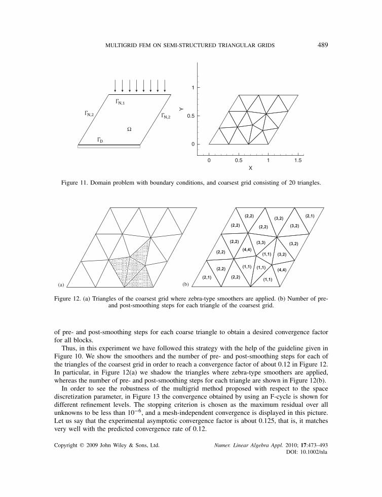
Figure 11. Domain problem with boundary conditions, and coarsest grid consisting of 20 triangles.

(a) (b)

Figure 12. (a) Triangles of the coarsest grid where zebra-type smoothers are applied. (b) Number of pre-and post-smoothing steps for each triangle of the coarsest grid.

of pre- and post-smoothing steps for each coarse triangle to obtain a desired convergence factorfor all blocks.

Thus, in this experiment we have followed this strategy with the help of the guideline given inFigure 10. We show the smoothers and the number of pre- and post-smoothing steps for each ofthe triangles of the coarsest grid in order to reach a convergence factor of about 0.12 in Figure 12.In particular, in Figure 12(a) we shadow the triangles where zebra-type smoothers are applied,whereas the number of pre- and post-smoothing steps for each triangle are shown in Figure 12(b).

In order to see the robustness of the multigrid method proposed with respect to the spacediscretization parameter, in Figure 13 the convergence obtained by using an F-cycle is shown fordifferent refinement levels. The stopping criterion is chosen as the maximum residual over allunknowns to be less than 10−6, and a mesh-independent convergence is displayed in this picture.Let us say that the experimental asymptotic convergence factor is about 0.125, that is, it matchesvery well with the predicted convergence rate of 0.12.



Figure 13. Multigrid convergence for the elasticity problem on thehomogeneous quadrilateral-shaped plate.

Figure 14. Wrench domain problem with boundary conditions.

4.2. 2D wrench problem

For this second example, we consider the homogeneous 2D wrench displayed in Figure 14, in whicha schematic representation of the boundary conditions is shown. The body is fixed on boundary�D, and on boundary �N=�N,1∪�N,2 a traction g=(g1,g2)t is applied, where (g1,g2)=(0,−1),on �N,1, and (g1,g2)=(0,0), on �N,2.

Twenty-nine triangles compose the coarsest grid as shown in Figure 15. In this picture, theobtained grid after two refinement levels is also depicted, and we can see that the more we refine,the more we approximate the grid to the real boundary of the domain. It is important to remarkhow the refinement is performed in the curved parts of the boundary in order to better fit thegeometry. As shown in Figure 16, the refinement of a triangle of the coarsest grid which hastwo vertices on the boundary of � is performed in the following way: the new boundary point istaken as the intersection of the perpendicular bisector of the edge with the corresponding boundaryarc. In general, this strategy may result in experimentally computed convergence factors slightlydifferent to those predicted by LFA, but this behavior has not been observed in this experiment.



Figure 15. Coarsest grid and grid obtained after two refinement levels.

P P

Figure 16. Refinement of the circular domain.

(a) (b)

Figure 17. (a) Triangles of the coarsest grid where zebra-type smoothers are applied. (b) Number of pre-and post-smoothing steps for each triangle of the coarsest grid.

As in the previous experiment, different smoothers and a different number of pre- and post-smoothing steps are considered for the triangles of the coarsest grid due to their different shapes.These have been chosen in order to obtain the desired convergence rate, which we have establishedas a convergence factor about 0.12. In Figure 17(a) the triangles where zebra smoothers are applied,are shown by shadowing them, and the number of pre- and post-smoothing steps for each triangleof the coarsest grid are depicted in Figure 17(b).

Thus, the multigrid method defined above has been applied to solve this problem by using anF-cycle, and the results are presented in Table VI. For different refinement levels, the numberof iterations necessary to reduce the initial residual with a factor of 10−10, and the asymptoticconvergence rates are shown, together with the number of elements and the number of unknowns ofthe problem. It is observed that the convergence is independent of the number of refinement levelsand the efficiency of this method is also seen, since the residual is reduced after 11 iterations of the



Table VI. Number of cycles and asymptotic convergence factors for different refinement levels.

No. of levels No. of elements No. of unknowns No. of cycles ( h)

5 7424 7700 11 (0.115)6 29696 30244 11 (0.125)7 118784 119876 11 (0.125)8 475136 477316 11 (0.125)9 1900544 1904900 11 (0.125)

10 7602176 7610884 11 (0.125)

multigrid algorithm. Again, it is observed that the obtained experimental asymptotic convergencefactor of about 0.125 fits very well the predicted one by LFA.

5. CONCLUSIONS

A stencil-based implementation of a geometric multigrid method on semi-structured grids hasbeen presented for linear finite element discretization of the problem of planar elasticity. A localFourier analysis for multigrid methods on triangular grids has been applied to this problem toselect adequate components of the algorithm. With the help of an LFA on triangular grids, athree-color smoother and some zebra-type smoothers have been proposed to obtain an efficientmultigrid algorithm to solve the planar elasticity problem, which is constructed in a block-wiseform. In particular, different smoothers and different numbers of pre- and post-smoothing stepsare considered in each triangle of the coarsest triangulation of the domain. The good performanceof this method has been shown by numerical experiments.

ACKNOWLEDGEMENTS

The authors thank the referees for their valuable comments which permitted us to improve the originalpaper. This research has been partially supported by FEDER/MCYT Projects MTM2007-63204 and theDGA (Grupo consolidado PDIE).

REFERENCES

1. Brandt A. Multigrid Techniques: 1984 Guide with Applications to Fluid Dynamics. GMD-Studie Nr. 85, SanktAugustin, Germany, 1984.

2. Hackbusch W. Multi-grid Methods and Applications. Springer: Berlin, 1985.3. Trottenberg U, Oosterlee CW, Schuller A. Multigrid. Academic Press: New York, 2001.4. Wesseling P. An Introduction to Multigrid Methods. Wiley: Chichester, U.K., 1992.5. Bergen B, Gradl T, Hulsemann F, Rude U. A massively parallel multigrid method for finite elements. Computing

in Science and Engineering 2006; 8:56–62.6. Brandt A. Multi-level adaptive solutions to boundary-value problems. Mathematics of Computation 1977; 31:

333–390.7. Wienands R, Joppich W. Practical Fourier Analysis for Multigrid Methods. Chapman & Hall, CRC Press: London,

Boca Raton, 2005.8. Niestegge A, Witsch K. Analysis of a multigrid Stokes solver. Applied Mathematics and Computation 1990;

35:291–303.9. Sivaloganathan S. The use of local mode analysis in the design and comparison of multigrid methods. Computer

Physics Communications 1991; 65:246–252.



10. Wienands R, Gaspar FJ, Lisbona FJ, Oosterlee CW. An efficient multigrid solver based on distributive smoothingfor poroelasticity equations. Computing 2004; 73:99–119.

11. Wittum G. Multi-grid methods for Stokes and Navier–Stokes equations with transforming smoothers: algorithmsand numerical results. Numerische Mathematik 1989; 54:543–563.

12. Mandel J, Ombe H. Fourier estimates for a multigrid method for three-dimensional elasticity. Multigrid Methods(Copper Mountain, CO, 1987). Lecture Notes in Pure and Applied Mathematics, vol. 110, 1988; 389–411.

13. Gaspar FJ, Gracia JL, Lisbona FJ. Fourier analysis for multigrid methods on triangular grids. SIAM Journal onScientific Computing 2009; 31:2081–2102.

14. Gaspar FJ, Gracia JL, Lisbona FJ, Rodrigo C. On geometric multigrid methods for triangular grids usingthree-coarsening strategy. Applied Numerical Mathematics 2009; 59:1693–1708.

15. Parsons ID, Hall JF. The multigrid method in solid mechanics: Part I—algorithm description and behaviour.International Journal for Numerical Methods in Engineering 1990; 29:719–737.

16. Parsons ID, Hall JF. The multigrid method in solid mechanics: Part II-Practical applications. International Journalfor Numerical Methods in Engineering 1990; 29:739–753.

17. Bastian P, Lang S, Eckstein K. Parallel adaptive multigrid methods in plane linear elasticity problems. NumericalLinear Algebra with Applications 1997; 4:153–176.

18. Ruge J. AMG for problems of elasticity. Applied Mathematics and Computation 1986; 19:293–309.19. Kocvara M, Mandel J. A multigrid method for three-dimensional elasticity and algebraic convergence estimates.

Applied Mathematics and Computation 1987; 23:121–135.20. Griebel M, Oeltz D, Schweitzer MA. An algebraic multigrid method for linear elasticity. SIAM Journal on

Scientific Computing 2003; 25:385–407.21. Kraus JK. Algebraic multigrid based on computational molecules, 2: linear elasticity problems. SIAM Journal

on Scientific Computing 2008; 30:505–524.22. Stuben K, Trottenberg U. Multigrid methods: fundamental algorithms, model problem analysis and applications.

In Multigrid Methods, Hackbusch W, Trottenberg U (eds). Lecture Notes in Mathematics, vol. 960. Springer:Berlin, 1982; 1–176.

23. Yavneh I. On red-black SOR smoothing in multigrid. SIAM Journal on Numerical Analysis 1996; 32:180–192.


Documents

Multigrid finite element methods on semi-structured triangular grids for planar elasticity