Multilevel Monte Carlo Approach for Estimating Reliability

Multilevel Monte Carlo Approach for Estimating Reliability

of Electric Distribution Systems

A. S. Nazmul Huda

Master of Science in Electrical and Electronic Engineering

Thesis submitted to the Faculty of Engineering, Computer and Mathematical

Sciences in total to fulfillment of the requirements for the degree of

Doctor of Philosophy

School of Electrical and Electronic Engineering

The University of Adelaide

Australia

-September 2018-

ii

iii

Abstract

Most of the power outages experienced by the customers are due to the failures in the

electric distribution systems. However, the ultimate goal of a distribution system is to meet

customer electricity demand by maintaining a satisfactory level of reliability with less

interruption frequency and duration as well as less outage costs. Quantitative evaluation of

reliability is, therefore, a significant aspect of the decision-making process in planning and

designing for future expansion of network or reinforcement.

Simulation approach of reliability evaluation is generally based on sequential Monte Carlo

(MC) method which can consider the random nature of system components. Use of MC

method for obtaining accurate estimates of the reliability can be computationally costly

particularly when dealing with rare events (i.e. when high accuracy is required). This thesis

proposes a simple and effective methodology for accelerating MC simulation in

distribution systems reliability evaluation. The proposed method is based on a novel

Multilevel Monte Carlo (MLMC) simulation approach.

MLMC approach is a variance reduction technique for MC simulation which can reduce

the computational burden of the MC method dramatically while both sampling and

discretisation errors are considered for converging to a controllable accuracy level. The

idea of MLMC is to consider a hierarchy of computational meshes (levels) instead of using

single time discretisation level in MC method. Most of the computational effort in MLMC

method is transferred from the finest level to the coarsest one, leading to substantial

computational saving. As the simulations are conducted using multiple approximations,

therefore the less accurate estimate on the preceding coarse level can be sequentially

corrected by averages of the differences of the estimations of two consecutive levels in the

hierarchy. In this dissertation, we will find the answers to the following questions: can

MLMC method be used for reliability evaluation? If so, how MLMC estimators for

reliability evaluation are constructed? Finally, how much computational savings can we

expect through MLMC method over MC method?

MLMC approach is implemented through solving the stochastic differential equations of

random variables related to the reliability indices. The differential equations are solved

using different discretisation schemes. In this work, the performance of two different

iv

discretisation schemes, Euler-Maruyama and Milstein are investigated for this purpose. We

use the benchmark Roy Billinton Test System as the test system. Based on the proposed

MLMC method, a number of reliability studies of distribution systems have been carried

out in this thesis including customer interruption frequency and duration based reliability

assessment, cost/benefits estimation, reliability evaluation incorporating different time-

varying factors such as weather-dependent failure rate and restoration time of components,

time-varying load and cost models of supply points. The numerical results that demonstrate

the computational performances of the proposed method are presented. The performances

of the MLMC and MC methods are compared. The results prove that MLMC method is

computationally efficient compared to those derived from standard MC method and it can

retain an acceptable level of accuracy. The novel computational tool including examples

presented in this thesis will help system planners and utility managers to provide useful

information of reliability of distribution networks. With the help of such tool they can take

necessary steps to speed up the decision-making process of reliability improvement.

v

Table of Contents

Abstract ................................................................................................................................ iii

Table of Contents ................................................................................................................. v

Statement of Originality .................................................................................................... vii

List of Publications ........................................................................................................... viii

Acknowledgements .............................................................................................................. x

Chapter 1: Introduction ...................................................................................................... 1

1.1. Background ................................................................................................................. 2

1.2. Distribution system reliability .................................................................................... 3

1.3. Reliability evaluation techniques ................................................................................ 4

1.4. Research gaps and objectives...................................................................................... 6

1.5. Details of manuscripts included in the thesis .............................................................. 7

References .......................................................................................................................... 9

Chapter 2: Simple Distribution System Reliability Evaluation..................................... 14

Statement of authorship ................................................................................................... 15

Improving distribution system reliability calculation efficiency using multilevel Monte

Carlo method .................................................................................................................... 16

Chapter 3: Comparative Reliability Study of Euler-Maruyama and Milstein Scheme

Based Methods ................................................................................................................... 39


Accelerated distribution systems reliability evaluation by multilevel Monte Carlo

simulation: Implementation of two discretisation schemes ............................................. 41

Chapter 4: Component Importance Analysis ................................................................. 64


Study components availability effect on distribution systems reliability through

Multilevel Monte Carlo method ...................................................................................... 66

Chapter 5: Interrupted energy estimation ...................................................................... 92

vi


Estimation of Expected Energy Not Supplied considering Time-Varying Load Models

by Multilevel Monte Carlo method: Effect of different factors on computation variation

......................................................................................................................................... 94

Chapter 6: Interruption Cost Estimation ...................................................................... 116

Statement of authorship ................................................................................................. 117

An efficient method with tunable accuracy for estimating expected interruption cost of

distribution systems ....................................................................................................... 118

Chapter 7: Effect of Weather Conditions on Computation ......................................... 146


Analysis effect of weather conditions on electric distribution system reliability

evaluation through an efficient approach ....................................................................... 148

Chapter 8: Study of Large-Scale DG Integration into Distribution Networks .......... 172


Large-scale penetration of distributed generation into distribution networks: Study

objectives, review of models and computational tools .................................................. 174

Chapter 9: Conclusions and Future Work .................................................................... 227

9.1. Summary ................................................................................................................. 228

9.2. Recommendations for future study ......................................................................... 231

vii

Statement of Originality

I certify that this work contains no material which has been accepted for the award of any

other degree or diploma in my name in any university or other tertiary institution and, to

the best of my knowledge and belief, contains no material previously published or written

by another person, except where due reference has been made in the text. In addition, I

certify that no part of this work will, in the future, be used in a submission in my name for

any other degree or diploma in any university or other tertiary institution without the prior

approval of The University of Adelaide and where applicable, any partner institution

responsible for the joint award of this degree.

I give consent to this copy of my thesis when deposited in the University Library, being

made available for loan and photocopying, subject to the provisions of the Copyright Act

1968.

The author acknowledges that copyright of published works contained within this thesis

resides with the copyright holder(s) of those works.

I also give permission for the digital version of my thesis to be made available on the web,

via the University's digital research repository, the Library Search and also through web

search engines, unless permission has been granted by the University to restrict access for

a period of time.

07.09.2018

A. S. Nazmul Huda Date

viii

List of Publications

Journal Papers:

1. A. S. Nazmul Huda and Rastko Živanović (2018) Study effect of components

availability on distribution system reliability through Multilevel Monte Carlo method,

IEEE Transactions on Industrial informatics. Published (Early access)

2. A. S. Nazmul Huda and Rastko Živanović (2017) Accelerated distribution systems

reliability evaluation by multilevel Monte Carlo simulation: Implementation of two

discretisation schemes, IET Generation, Transmission & Distribution, 11(13), 3397-

3405.

3. A. S. Nazmul Huda and R. Živanović (2019) An efficient method with tunable

accuracy for estimating expected interruption cost of distribution systems, International

Journal of Electrical Power & Energy Systems, 105, 98-109. [Elsevier]

4. A.S.N. Huda and Rastko Živanović (2017) Improving distribution system reliability

calculation efficiency using multilevel Monte Carlo method, International Transactions

on Electrical Energy Systems, 27(7), 1-12. [Wiley]

5. A.S.N. Huda and R. Živanović (2017) Large-scale penetration of distributed

generation into distribution networks: Study objectives, review of models and

computational tools, Renewable and Sustainable Energy Reviews, 76, 974-988.

[Elsevier]

6. A. S. Nazmul Huda and Rastko Živanović (2018) Estimation of Expected Energy

Not Supplied considering Time-Varying Load Models by Multilevel Monte Carlo

method: Effect of different factors on computation variation, Electric Power

Components and Systems. Submitted revision. [Taylor & Francis]

7. A. S. Nazmul Huda and R. Živanović (2018) Analysis effect of weather conditions

on electric distribution system reliability evaluation through an efficient approach,

Quality and Reliability Engineering International. Received feedback from reviewers.

[Wiley]

ix

Conference Papers:

1. A. S. Nazmul Huda and Rastko Živanović, Efficient estimation of interrupted

energy with time varying load models for distribution systems planning studies, 9th

Vienna International Conference on Mathematical Modelling, 21-23 February 2018,

Vienna, Austria.

2. A. S. Nazmul Huda and Rastko Živanović, Advanced computation method for

value-based distribution systems reliability evaluation, 15th Symposium on Energy

Innovation, 14-16 February 2018, Graz, Austria.

3. A. S. N. Huda and Rastko Živanović, Multilevel Monte Carlo method applied to

distribution system reliability assessment, IEEE PES PowerTech, 18-22 June 2017,

Manchester, UK, pp. 1-6.

4. A.S.N. Huda and Rastko Živanović, Distribution system reliability assessment using

sequential multilevel Monte Carlo method, IEEE PES Innovative Smart Grid

Technologies- Asia (ISGT-Asia), 28-01 December 2016, Melbourne, Australia, pp.

867-872.

5. A. S. Nazmul Huda and Rastko Živanović, Advanced simulation method for

evaluation of interrupted energy assessment rates in distribution systems, Australasian

Universities Power Engineering Conference, 27-30 November 2018, Auckland.

Accepted.

6. A. S. Nazmul Huda & Rastko Živanović (2018) An efficient method for distribution

system reliability evaluation incorporating weather dependent factors, 20th

IEEE

International Conference on Industrial Technology, February 13-15 2019, Melbourne.

Accepted.

x

Acknowledgements

First of all, the author would like to thank the Almighty Allah for granting him the ability

to complete his PhD study.

The author wishes to acknowledge the contribution of his supervisor Dr. Rastko Živanović

for his valuable, constructive supervision and continuous support throughout his research

and preparation of this thesis.

Thanks are also extended to Dr. Said Al-Sarawi and Dr. Wen Soong for their suggestion

and support.

Financial support provided by The University of Adelaide is gratefully acknowledged.

Finally, the author would like to express his deepest gratitude to his parents, wife,

daughter, sisters and their families, all the relatives and friends for their love, patience and

support throughout his studies.

xi

Chapter 1

Introduction

2

1.1. Background

In an electric power system, electricity is generated, transmitted and distributed to the end

users through generation, transmission and distribution systems, respectively. Distribution

system is the last portion which delivers electricity from the transmission system to the

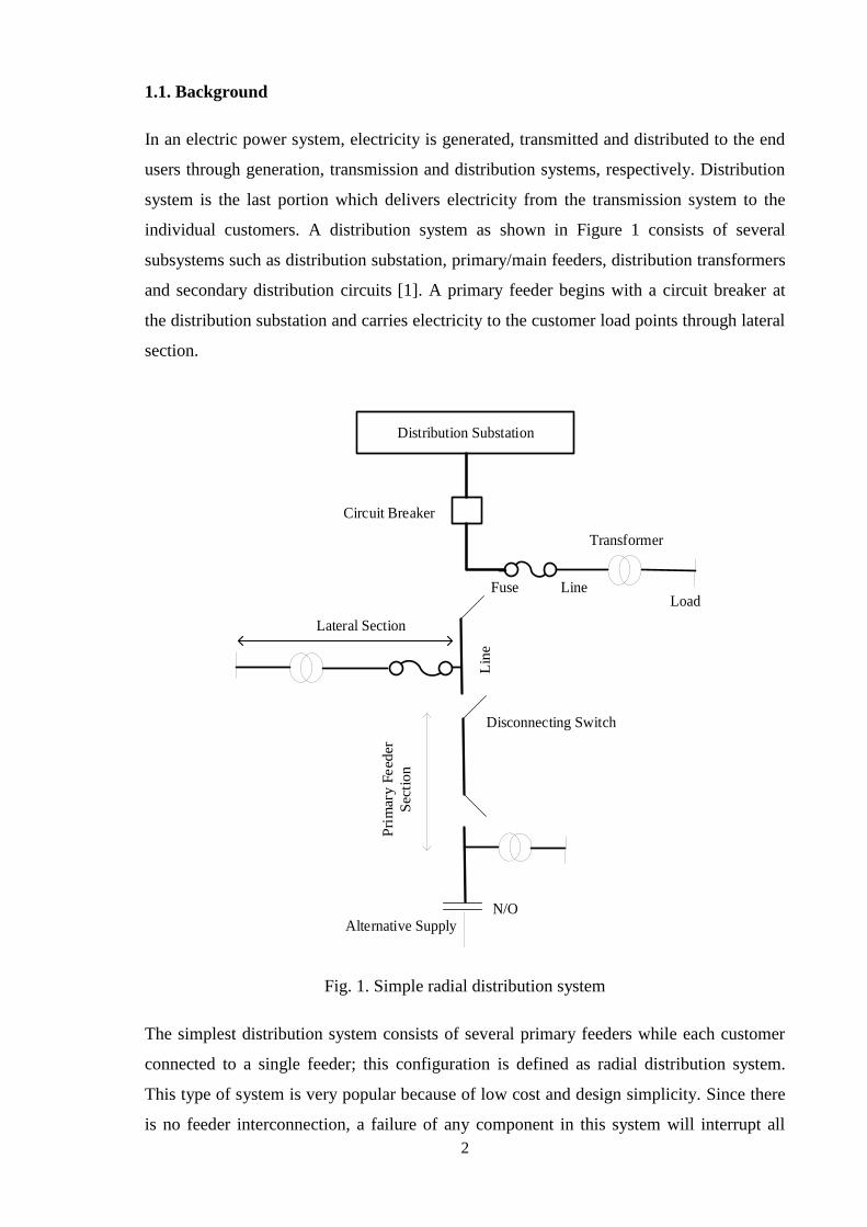
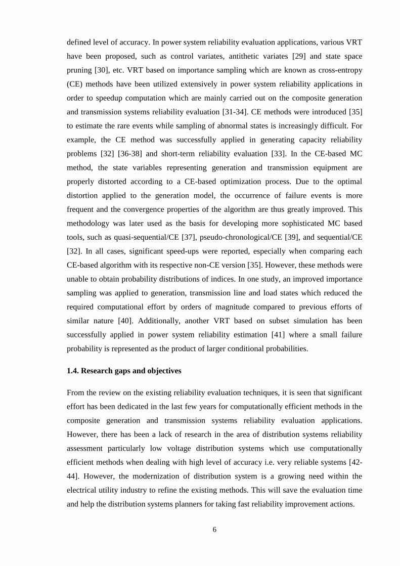
individual customers. A distribution system as shown in Figure 1 consists of several

subsystems such as distribution substation, primary/main feeders, distribution transformers

and secondary distribution circuits [1]. A primary feeder begins with a circuit breaker at

the distribution substation and carries electricity to the customer load points through lateral

section.

Distribution Substation

Circuit Breaker

Fuse

Transformer

Load

N/O

Disconnecting Switch

Lateral Section

Pri

mar

y F

eed

er

Sec

tion

Line

Lin

e

Alternative Supply

Fig. 1. Simple radial distribution system

The simplest distribution system consists of several primary feeders while each customer

connected to a single feeder; this configuration is defined as radial distribution system.

This type of system is very popular because of low cost and design simplicity. Since there

is no feeder interconnection, a failure of any component in this system will interrupt all

3

downstream customers until it is cleared. There are a set of series components available

between the substation and the customer load points as shown in Figure 1.

A general main section consists of disconnecting switches and a transmission line.

Disconnecting switches can isolate the faulted part of the network by switching of

sectionalizing equipment and supply power to the customers of unfaulty part if there is an

availability of any alternative supply source, while the faulted component is being repaired.

This reduces the outage duration and number of affected customers during failure. A

general lateral section includes the basic components such as distribution transformer,

transmission line and fuse. The availability of lateral fuse clears any fault on the lateral

section or in the transformer and thus maintains the service of the primary feeder. If in any

case, the fuse fails to restore the service, the circuit breaker or the back-up fuse on the

primary feeder acts to isolate the faulted lateral section and the supply is then restored to

the remaining system by closing the circuit breaker [2].

1.2. Distribution system reliability

The function of an electric distribution system is to deliver electricity to the customers

without supply interruptions. The ability of a distribution system to fulfill the customer

load requirement with continuity is usually defined as reliability. 100 percent reliable

system delivers power to the customers without any interruption. Data on utility failure

statistics show that distribution system failures are the causes of approximately 80 percent

of the total customer interruptions which result from problems occurring between load

points and distribution substations [3]. In a typical working condition, all components in a

distribution system are energized. Therefore, customers are supplied power without any

interruption. Scheduled and unscheduled events disrupt the regular operations and could

lead to components failure and service interruption. The evaluation of reliability of a

distribution system reveals the level of ability of system which depends on the components

performance about how perfectly they perform their intended function. Through the

evaluation, areas of high or low level of reliability can be recognized by identifying faulty

equipment that degrades system reliability. The model can help to quantify the impact of

design improvement options which includes [4]:

(a) New feeders and feeder expansion,

(b) Load transfer between feeders,

(c) New substation and substation expansion,

(d) New feeder tie points,

4

(e) Line reclosers,

(f) Sectionalizing switches,

(g) Feeder automation,

(h) Replacement of aging equipment and

(i) Replacing overhead circuits by underground cables.

In the evaluation, we measure or calculate some indices of interruption frequency and

duration based on network configuration, connected components failure and restoration

data and loading condition, etc. This evaluation can support a distribution system planner

to access most of the required knowledge about expected frequency, duration, cost and

energy loss of interruptions. The reliability measures are typically divided into measures of

the impact of momentary and sustained interruptions to the supply [5]. Sustained

interruption means an interruption to a distribution customer’s electricity supply that has

duration longer than three minutes [6]. Interruption duration is the time period starting

from the initiation of interruption until supply has been provided or restored to the affected

customers. The impact of a sustained interruption on customers is usually significantly

more than that of a momentary interruption. Momentary interruption means an interruption

to distribution customers’ electricity supply with duration of three minutes or less. The

impact of momentary interruptions on customers could be that their lights go off and return

back on shortly. Some recommended indices for the sustained interruptions are System

Average Interruption Frequency Index (SAIFI), System Average Interruption Duration

Index (SAIDI) and Customer Average Interruption Duration Index (CAIDI), etc. [7] while

the measures for momentary interruptions are Momentary Average Interruption Frequency

Index (MAIFI) and Momentary Average Interruption Event Frequency Index (MAIFIE),

etc. [6].

1.3. Reliability evaluation techniques

Two basic techniques are generally used to evaluate the reliability of a system: analytical

and simulation techniques [8-10]. Analytical technique calculates only expected values of

the reliability indices based on the historical data. Analytical techniques are mainly based

on Failure Mode and Effect Analysis (FMEA) [11] [12], minimal path sets [13], minimal

cut sets [14], Bayesian network methods [15], etc. The technique does not consider the

random behavior of the reliability indices. However, the calculation of indices is based on

two basic random parameters, i.e. time-to-failure and time-to-restoration and therefore the

reliability indices are generally random in nature. Thus while estimating a reliability index;

5

it is important to consider the amount of deviation (i.e. upper and lower bounds) from an

average value based on specified probability distribution for system expansion and future

planning. Additionally, the need of analysis of different probabilistic factors in accurate

reliability modelling is a very important task for complex modern distribution systems.

Therefore, reliability analysts require the use of other technique which is accurate, efficient

and can consider the random nature of reliability indices.

Monte Carlo (MC) method is the widely used simulation approach which allow the

solution of mathematical and technical problems by means of system probabilistic models

and simulation of random variables [16]. It is used to determine an estimate of the expected

value of a parameter of interest and analyse systems whose variables follow various

probability distributions such as binomial, exponential, Weibull, lognormal and gamma,

etc. Therefore, it has been used for many years in different areas of science and

engineering. Like other applications, MC simulation approach has been extensively used

for many years in power system reliability evaluation applications [17-23]. It can be

simulated in either a sequential or a non-sequential mode [24]. In the non-sequential

mode, the states of all components are sampled and a non-chronological system state is

obtained [25]. The sequential MCS is able to reproduce the chronological evolution of the

system by sampling stochastic sequences of system states. These sequences are simulated

based on the stochastic modeling of each system component failure and restoration cycles

and overall system operating cycle is achieved by combining all the components cycles

[25]. The sequential MC allows the consideration of the chronological matters and

distributions of the reliability indices [26]. The state duration sampling approach is

generally used to simulate chronological issues which can describe time-related reliability

indices concerning frequency and duration of interruption [27]. The most attractive feature

of MC simulation method is that the required number of samples for a target convergence

criterion is not dependent on the number of number of buses in the power system [28].

However, a disadvantage of the sequential MC method is that it is very time-consuming

when dealing with a highly reliable system with probabilities of very smaller occurrence.

Therefore, the number of required samples increases with respect to the desired high

accuracy level of the estimates and hence the practicability of this approach is decreased

for a very reliable system.

In order to enhance the convergence speed of the MC method, variance reduction

techniques (VRT) are generally used. Through VRT, the expected value of an output

random variable can be obtained with reduced computation time by maintaining a pre-

6

defined level of accuracy. In power system reliability evaluation applications, various VRT

have been proposed, such as control variates, antithetic variates [29] and state space

pruning [30], etc. VRT based on importance sampling which are known as cross-entropy

(CE) methods have been utilized extensively in power system reliability applications in

order to speedup computation which are mainly carried out on the composite generation

and transmission systems reliability evaluation [31-34]. CE methods were introduced [35]

to estimate the rare events while sampling of abnormal states is increasingly difficult. For

example, the CE method was successfully applied in generating capacity reliability

problems [32] [36-38] and short-term reliability evaluation [33]. In the CE-based MC

method, the state variables representing generation and transmission equipment are

properly distorted according to a CE-based optimization process. Due to the optimal

distortion applied to the generation model, the occurrence of failure events is more

frequent and the convergence properties of the algorithm are thus greatly improved. This

methodology was later used as the basis for developing more sophisticated MC based

tools, such as quasi-sequential/CE [37], pseudo-chronological/CE [39], and sequential/CE

[32]. In all cases, significant speed-ups were reported, especially when comparing each

CE-based algorithm with its respective non-CE version [35]. However, these methods were

unable to obtain probability distributions of indices. In one study, an improved importance

sampling was applied to generation, transmission line and load states which reduced the

required computational effort by orders of magnitude compared to previous efforts of

similar nature [40]. Additionally, another VRT based on subset simulation has been

successfully applied in power system reliability estimation [41] where a small failure

probability is represented as the product of larger conditional probabilities.

1.4. Research gaps and objectives

From the review on the existing reliability evaluation techniques, it is seen that significant

effort has been dedicated in the last few years for computationally efficient methods in the

composite generation and transmission systems reliability evaluation applications.

However, there has been a lack of research in the area of distribution systems reliability

assessment particularly low voltage distribution systems which use computationally

efficient methods when dealing with high level of accuracy i.e. very reliable systems [42-

44]. However, the modernization of distribution system is a growing need within the

electrical utility industry to refine the existing methods. This will save the evaluation time

and help the distribution systems planners for taking fast reliability improvement actions.

7

The main objective of this thesis is therefore to present the computationally efficient

estimation and accurate models. For this purpose, a novel Multilevel Monte Carlo

(MLMC) method based reliability evaluation technique has been proposed. MLMC

approach is a variance reduction technique for MC simulation which can reduce the

computational burden of the MC method dramatically while both sampling and

discretisation errors are considered for converging to a controllable accuracy level. Based

on the proposed MLMC method, a number of reliability studies of distribution systems

have been carried out in this thesis including customer interruption frequency and duration

based reliability assessment, reliability cost/benefits estimation, reliability evaluation

incorporating different time-varying factors such as weather-dependent failure rate and

restoration time of components, time-varying load and cost models of supply points. The

numerical results that demonstrate the computational performances of the proposed method

are presented. The performances of the MLMC and MC methods are compared.

1.5. General overview of the thesis

This thesis contains a number of manuscripts which are submitted and accepted to

internationally recognized journals. Each chapter of the thesis is presented in the form of a

journal paper which is self-sufficient individually and do not need the accumulation of

information from the previous chapters.

Chapter 2 presents the application of MLMC method which is implemented for reliability

evaluation of a small distribution system. The Milstein path discretisation is used to

approximate the numerical solution of stochastic equations. Case studies are carried to

evaluate the basic system performance indices.

Chapter 3 presents a study on reliability evaluation of benchmark test distribution

systems. The convergence characteristics of MLMC methods based on two discretisation

schemes, i.e. Euler-Maruyama and Milstein discretisation schemes are investigated in this

chapter. The Roy Billinton Test Systems are used as benchmark distribution systems.

Chapter 4 investigates the effect of basic protection components availability, failure and

restoration parameters on reliability improvement. The effect of components availability

on reliability indices for overall system, feeders and customer sector types are evaluated

through the MLMC method. Additionally, sensitivity analyses are performed to show the

impact of variation of the predefined reliability data and the MLMC parameters on

computational performance.

8

Chapter 5 presents the MLMC based estimation results of system expected energy not

supplied index by incorporating different time-varying load models. The Euler-Maruyama

discretisation method is coupled with the MLMC method to develop a general framework

for this estimation. The second objective is to explore the effect of various factors and

criteria on computation performance such as failure starting time, failure duration, time-

dependent load diversity factors, network complexity, systems reinforcement, target

accuracy level and discretisation scheme. The outputs of the MLMC method are compared

with the direct MCS from the accuracy and computational speed perspectives.

Chapter 6 investigates the application of MLMC method on estimating the system

expected interruption cost. The performance of the proposed method is compared with the

MC method in terms of computation accuracy and speed-up. The effect of different

parameters on the MLMC computation method such as network configuration and load

type, time-varying load and cost models, network reinforcement, transformer and line

failure rate, drift and volatility values are investigated to provide insight into the variation

of the interruption cost with different system factors.

Chapter 7 establishes a time sequential MLMC simulation for the reliability indices

calculation of distribution systems in two different weather conditions. For modelling time-

varying failure rate, weather dependent factors such as high wind speed and lightning are

considered in reliability estimation. Different time-varying weight factors and a delay

during adverse weather are considered in modelling of restoration time. Similarly, for load

and cost modelling, different time-varying weight factors are incorporated in calculation. A

comprehensive result showing the effects of different time-varying parameter models are

presented while the computations are performed using MLMC method. The computation

accuracy compared to the original MC method is also presented.

In terms of the improvement of reliability and efficiency, integration of distributed

generation (DG) into distribution network has gained significant interest in recent years.

However, existing distribution systems were not designed considering penetration of DG.

Chapter 8 reviews the required models of system components, the impacts of DG on

system operation, mitigation of challenges, associated standards and regulations for the

successful operation of distribution systems. The second objective is to make a summary of

characteristics and features that an ideal computational tool should have to study increased

DG penetration. A comparison study of two commonly used computational tools is also

carried out in this paper.

9

References

[1] R. E. Brown, Electric power distribution reliability: CRC press, 2008.

[2] W. Li, Reliability assessment of electric power systems using Monte Carlo

methods: Springer Science & Business Media, 2013.

[3] R. Billinton and J. Billinton, “Distribution system reliability indices,” IEEE

Transactions on Power Delivery, vol. 4, pp. 561-568, 1989.

[4] T. Gonen, Electric power distribution engineering: CRC press, 2016.

[5] T. H. Ortmeyer, J. A. Reeves, D. Hou, and P. McGrath, “Evaluation of sustained

and momentary interruption impacts in reliability-based distribution system

design,” IEEE Transactions on Power Delivery, vol. 25, pp. 3133-3138, 2010.

[6] J. Nahman and D. Peric, “Distribution system performance evaluation accounting

for data uncertainty,” IEEE Transactions on Power Delivery, vol. 18, pp. 694-700,

2003.

[7] R. E. Brown and J. R. Ochoa, “Distribution system reliability: default data and

model validation,” IEEE Transactions on Power Systems, vol. 13, pp. 704-709,

1998.

[8] Y. Ou and L. Goel, “Using Monte Carlo simulation for overall distribution system

reliability worth assessment,” IEE Proceedings-Generation, Transmission and

Distribution, vol. 146, pp. 535-540, 1999.

[9] R. Billinton and P. Wang, “Distribution system reliability cost/worth analysis using

analytical and sequential simulation techniques,” IEEE Transactions on Power

Systems, vol. 13, pp. 1245-1250, 1998.

[10] A. Volkanovski, M. Čepin, and B. Mavko, “Application of the fault tree analysis

for assessment of power system reliability,” Reliability Engineering & System

Safety, vol. 94, pp. 1116-1127, 2009.

[11] R. N. Allan, R. Billinton, I. Sjarief, L. Goel, and K. So, “A reliability test system

for educational purposes-basic distribution system data and results,” IEEE

Transactions on Power systems, vol. 6, pp. 813-820, 1991.

[12] R. Billinton and P. Wang, “Reliability-network-equivalent approach to distribution-

system-reliability evaluation,” IEE Proceedings-Generation, Transmission and

Distribution, vol. 145, pp. 149-153, 1998.

10

[13] K. Xie, J. Zhou, and R. Billinton, “Reliability evaluation algorithm for complex

medium voltage electrical distribution networks based on the shortest path,” IEE

Proceedings-Generation, Transmission and Distribution, vol. 150, pp. 686-690,

2003.

[14] X. Xiang and Y. Hao, “Reliability Evaluation of Distribution Systems Based on the

Minimum Cut Sets Method,” Journal of Electric Power, vol. 21, pp. 149-153,

2006.

[15] D. C. Yu, T. C. Nguyen, and P. Haddawy, “Bayesian network model for reliability

assessment of power systems,” IEEE Transactions on Power Systems, vol. 14, pp.

426-432, 1999.

[16] C. P. Robert, Monte carlo methods: Wiley Online Library, 2004.

[17] Y. Ou and L. Goel, “Using Monte Carlo simulation for overall distribution system

reliability worth assessment,” IEE Proceedings-Generation, Transmission and

Distribution, pp. 535-540, 1999.

[18] L. Goel and Y. Ou, “Reliability worth assessment in radial distribution systems

using the Monte Carlo simulation technique,” Electric power systems research, vol.

51, pp. 43-53, 1999.

[19] L. Goel, “Monte Carlo simulation-based reliability studies of a distribution test

system,” Electric Power Systems Research, vol. 54, pp. 55-65, 2000.

[20] R. Billinton and P. Wang, “Teaching distribution system reliability evaluation

using Monte Carlo simulation,” IEEE Transactions on Power Systems, vol. 14, pp.

397-403, 1999.

[21] Y. Hegazy, M. Salama, and A. Chikhani, “Adequacy assessment of distributed

generation systems using Monte Carlo simulation,” IEEE Transactions on Power

Systems, vol. 18, pp. 48-52, 2003.

[22] R. Rocchetta, Y. Li, and E. Zio, “Risk assessment and risk-cost optimization of

distributed power generation systems considering extreme weather conditions,”

Reliability Engineering & System Safety, vol. 136, pp. 47-61, 2015.

[23] L. Goel and Y. Ou, “Radial distribution system reliability worth evaluation utilizing

the Monte Carlo simulation technique,” Computers & Electrical Engineering, vol.

27, pp. 273-285, 2001.

11

[24] J. A. Momoh, Electric power distribution, automation, protection, and control:

CRC press, 2007.

[25] W. Li, Risk assessment of power systems: models, methods, and applications: John

Wiley & Sons, 2014.

[26] R. Billinton and A. Sankarakrishnan, “A comparison of Monte Carlo simulation

techniques for composite power system reliability assessment,” In: IEEE

Conference on Communications, Power, and Computing, 1995, pp. 145-150.

[27] R. Billinton and W. Li, “Distribution System and Station Adequacy Assessment,”

in Reliability assessment of electric power systems using Monte Carlo methods,

Springer, 1994, pp. 209-254.

[28] B. Zhaohong and W. Xifan, “Studies on variance reduction technique of Monte

Carlo simulation in composite system reliability evaluation,” Electric Power

Systems Research, vol. 63, pp. 59-64, 2002.

[29] R. Billinton and A. Jonnavithula, “Composite system adequacy assessment using

sequential Monte Carlo simulation with variance reduction techniques,” IEE

Proceedings-Generation, Transmission and Distribution, vol. 144, pp. 1-6, 1997.

[30] C. Singh and J. Mitra, “Composite system reliability evaluation using state space

pruning,” IEEE Transactions on Power Systems, vol. 12, pp. 471-479, 1997.

[31] K. Hou, H. Jia, X. Xu, Z. Liu, and Y. Jiang, “A continuous time Markov chain

based sequential analytical approach for composite power system reliability

assessment,” IEEE Transactions on Power Systems, vol. 31, pp. 738-748, 2016.

[32] R. A. González-Fernández and A. M. L. da Silva, “Reliability assessment of time-

dependent systems via sequential cross-entropy Monte Carlo simulation,” IEEE

Transactions on Power Systems, vol. 26, pp. 2381-2389, 2011.

[33] Y. Wang, C. Guo, and Q. Wu, “A cross-entropy-based three-stage sequential

importance sampling for composite power system short-term reliability

evaluation,” IEEE Transactions on Power Systems, vol. 28, pp. 4254-4263, 2013.

[34] A. S. N. Huda and R. Zivanovic, “Accelerated Distribution Systems Reliability

Evaluation by Multilevel Monte Carlo Simulation: Implementation of Two

Discretisation Schemes,” IET Generation, Transmission & Distribution, vol. 11,

pp. 3397-3405, 2017.

12

[35] R. A. González-Fernández, A. M. L. da Silva, L. C. Resende, and M. T. Schilling,

“Composite systems reliability evaluation based on Monte Carlo simulation and

cross-entropy methods,” IEEE Transactions on Power Systems, vol. 28, pp. 4598-

4606, 2013.

[36] A. M. L. da Silva, R. A. Fernandez, and C. Singh, “Generating capacity reliability

evaluation based on Monte Carlo simulation and cross-entropy methods,” IEEE


[37] A. M. L. da Silva, R. A. González-Fernández, W. S. Sales, and L. A. Manso,

“Reliability assessment of time-dependent systems via quasi-sequential Monte

Carlo simulation,” In: IEEE 11th International Conference on Probabilistic

Methods Applied to Power Systems (PMAPS), 2010, pp. 697-702.

[38] R. González-Fernández and A. L. Da Silva, “Comparison between different cross-

entropy based methods applied to generating capacity reliability,” In: IEEE 11th

International Conference on Probabilistic Methods Applied to Power Systems

(PMAPS), 2012, pp. 10-14.

[39] A. L. Da Silva, L. D. F. Manso, J. D. O. Mello, and R. Billinton, “Pseudo-

chronological simulation for composite reliability analysis with time varying

loads,” IEEE Transactions on Power Systems, vol. 15, pp. 73-80, 2000.

[40] E. Tomasson and L. Söder, “Improved importance sampling for reliability

evaluation of composite power systems,” IEEE Transactions on Power Systems,

vol. 32, pp. 2426-2434, 2017.

[41] B. Hua, Z. Bie, S.-K. Au, W. Li, and X. Wang, “Extracting rare failure events in

composite system reliability evaluation via subset simulation,” IEEE Transactions

on Power Systems, vol. 30, pp. 753-762, 2015.

[42] G. T. Heydt and T. J. Graf, “Distribution system reliability evaluation using

enhanced samples in a Monte Carlo approach,” IEEE Transactions on Power

Systems, vol. 25, pp. 2006-2008, 2010.

[43] F. Li, “A fast approach of Monte Carlo simulation based on linear contribution

factors to distribution reliability indices,” In: IEEE PES Transmission and

Distribution Conference and Exposition, 2003, pp. 973-977.

[44] R. Arya, A. Tiwary, S. Choube, and L. Arya, “A smooth bootstrapping based

technique for evaluating distribution system reliability indices neglecting random

13

interruption duration,” International Journal of Electrical Power & Energy

Systems, vol. 51, pp. 307-310, 2013.

14

Chapter 2

Simple Distribution System Reliability Evaluation

15

Statement of authorship

Title of Paper Improving distribution system reliability calculation efficiency using multilevel Monte Carlo

method

Publication Status Published

Accepted for Publication

Submitted for Publication

Unpublished and Unsubmitted w ork w ritten in

manuscript style

Publication Details A.S.N. Huda and Rastko Živanović (2017) Improving distribution system reliability calculation

efficiency using multilevel Monte Carlo method, International Transactions on Electrical Energy

Systems, 27(7), pp. 1-12.

Link: https://onlinelibrary.wiley.com/doi/full/10.1002/etep.2333

Principal author

Name of Principal Author

(Candidate)

A. S. Nazmul Huda

Contribution to the Paper

Development of reliability evaluation model, performed simulation and numerical analysis,

preparation of manuscript.

Overall percentage (%) 80%

Certification: This paper reports on original research I conducted during the period of my Higher Degree by

Research candidature and is not subject to any obligations or contractual agreements with a

third party that would constrain its inclusion in this thesis. I am the primary author of this

paper.

Signature

Date 07.09.2018

Co-author contributions

By signing the Statement of Authorship, each author certifies that:

the candidate’s stated contribution to the publication is accurate (as detailed above);

permission is granted for the candidate in include the publication in the thesis; and

the sum of all co-author contributions is equal to 100% less the candidate’s stated contribution.

Name of Co-Author Rastko Živanović

Contribution to the Paper Supervised for development of model, helped in data interpretation and manuscript evaluation

Signature Date 13.08.2018

https://onlinelibrary.wiley.com/doi/full/10.1002/etep.2333

16

Improving distribution system reliability calculation efficiency using multilevel

Monte Carlo method

Summary- Power distribution system reliability is generally evaluated by sequential

Monte Carlo simulation (MCS). To obtain a high accuracy, sequential MCS technique

needs long execution time. In this paper, we show that reliability indices could be

evaluated using a novel sequential multilevel Monte Carlo (MLMC) technique that

improves the computational efficiency of MCS. The key idea behind the MLMC method is

to use computationally cheaper low accuracy solutions of coarse grids as control variates

for high accuracy solutions of fine grids. Therefore, the proposed method can construct

multilevel estimators of reliability indices with lower variance. Reliability indices are

modelled based on stochastic differential equations (SDE) and exponential probability

distributions. The Milstein path discretisation is used to approximate the numerical

solution of SDE. Case studies are carried out on a small distribution system. Numerical

results are presented to demonstrate the computational cost-effectiveness of the proposed

method in comparison to the sequential MCS.

Keywords—distribution system; reliability; multilevel Monte Carlo (MLMC); Milstein

discretisation; computational efficiency

1. Introduction

Utility statistics show that more than 80 percent of the customer service interruptions occur

due to the malfunction of distribution system components [1]. Therefore, electric utilities

require improving the reliability of distribution system. Reliability assessment models of

distribution systems could be useful to predict the system performance based on basic

system topology and components reliability statistics. This assessment may help the system

planners to develop necessary strategies [2, 3] for supplying power to the customers with

the lowest possible interruptions and costs.

Methods for reliability assessment of distribution systems are generally divided into

analytical and simulation categories. Analytical technique is basically based on component

failure mode and effect analysis [4]. It can provide only the average values of the load

point and system performance indices. This drawback of analytical approach can be

overcome using the simulation approach which can provide both the average values and

probability distributions of the load point and system indices. Time sequential Monte Carlo

(MC) method based simulation techniques [5-14] have been extensively used in

17

distribution system reliability assessment. In a sequential simulation, artificial operating

and restoration histories of system components are generated in chronological order using

random number generators and components failure and restoration parameters. Using the

operating and restoration histories of system components, the load point reliability indices

and furthermore, overall system performance indices are determined. Since the calculations

of the reliability indices are conducted using a large number of samples based on the

desired accuracy, therefore it may require longer computation time to obtain a high

accuracy.

The increased number of time-dependent random variables and system configurations

complexities greatly increase the computation time of reliability assessment. The demand

of reduction of computational complexity by maintaining the accuracy within an

acceptable level is increasing day by day. By this way, the whole process will be faster and

system planners can take necessary steps to speed up the process of reliability

improvement. A lot of researches have been conducted to reduce the computation time in

the planning problems [15-21]. In this study, a new variance reduction technique based on

multilevel Monte Carlo (MLMC) method has been proposed to apply in distribution

system reliability assessment.

The idea of MLMC method was first initiated by Heinrich [22] to improve the

computational efficiency for high-dimensional parameter-dependent integrals. Then Brandt

and Ilyin [23] used the method to speed up the statistical mechanical computations. The

idea was later extended by Giles [24] to reduce the computational burden of estimating an

expected value arising from stochastic differential equations (SDE) in mathematical

finance. Since then, it has been applied in numerous areas [25-29] of solving SDE and

stochastic partial differential equations (SPDE) with random variables. From these studies,

the computational cost effectiveness of MLMC over MC method has been proved. In this

study, we intend to apply the method in a new area which is electric distribution system to

evaluate the uncertain random reliability indices.

In MC method, numerical models of reliability indices are simulated on the finest grid

level. In the finest grid, simulation error is small but the computational cost of execution is

very large. In MLMC method, same quantities are defined but using a geometric sequence

of coarse grids, rather than only the finest grid. On a coarse grid, both the computational

cost and simulation accuracy are reduced. Thus, the overall computational cost is reduced

using this method. Since the method conducts the simulations on a sequence of coarse

18

grids, so less accurate approximation on the previous coarser grid can be sequentially

corrected by evaluations on the following finer grids. Therefore, MLMC method can

achieve the same accuracy as MC method. In this study, we explain how the computational

cost is saved by MLMC in computing distribution system reliability indices.

In the current study, distribution system components are assumed to be represented by two-

state models [30]. Time-to-failure (TTF) and time-to-repair (TTR) of a component are

random variables [31] and these are simply approximations of the actual failure and repair

time, respectively. Distribution system reliability is generally assessed with the useful life

period of the component. The failure rate of a component is assumed as constant and

exponential probability distribution is usually employed for modelling the uncertainty of

TTF [32, 33]. Similarly, in this study, repair time is also assumed as constant and

exponential distribution could be used for modelling TTR randomness. The MLMC

method could be used in reliability evaluation by constructing the SDE based modelling of

component TTF and TTR. Therefore, in the proposed method, a combination of SDE and

exponential probability distributions [34, 35] based modelling of random variables is

utilised for the approximation of the component's actual failure and repair time [31]. The

Milstein path discretisation is used to approximate the numerical solution of SDE. Then,

time sequential MLMC method is developed to determine the reliability indices.

The paper begins by discussing the basics of MC and MLMC methods. In this section, we

summarise the difference between the two methods. Section 3 explains the methodology of

reliability assessment based on the proposed method. Section 4 represents the case studies

and associated simulation results to demonstrate the capability of MLMC method in

distribution system reliability evaluation. Case studies are carried out on a simple

distribution system to evaluate three basic system performance indices: system average

interruption frequency index (SAIFI), system average interruption duration index (SAIDI)

and customer average interruption duration index (CAIDI).

2. Detailed explanation of MC and MLMC methods

2.1. MC method

In this section, we will discuss the estimation of using MC simulations. For this

study, we can define as follows:

19

(1)

In MCS, is estimated by using an expected value of a random variable.

can be approximated by averaging over a large number of samples on a single fine level

from the distribution of [36]. If

is the ith sample of and is the number of

Monte Carlo samples. Then, the MCS estimator for is

(2)

Mean square error (MSE) is used to measure the accuracy of the MC estimator and is

defined as follows [27]:

(3)

The first term of the MSE in (3) is the sampling error which is represented by the variance

of the MC estimator. This error is small as is small and decays inversely with the

number of samples . The second term is the square of the error in the mean value

between and , which can be reduced by using a high accuracy fine grid. To achieve a

root mean square error (RMSE) of with the MC estimator, we need to have

i.e., both of the errors should be less than [37]. To achieve this

accuracy, we require samples. Here, we simply expressed the complexity

of Equation (3) through the relationship between the number of Monte Carlo samples and

accuracy level using big O notation. Therefore, for the estimator being a sufficiently

accurate approximation of with a small , a large number of samples need to be

simulated. This results in huge computational cost.

2.2. MLMC method

In MCS, all the samples are simulated on the finest level L using a specific timestep where

we just sample one approximation of . In MLMC method, we use several

approximations of . We estimate the approximations on different levels using a

different timestep for each level. Starting from the coarsest level to the finest level

, the proposed method uses a sequence of levels . Mathematically, the

idea of MLMC can be written as follows [24]:

(4)

20

In this method, the expectation on the finest level is equal to the expectation on the

coarsest level plus a sum of corrections which give the difference in expectation between

the simulations using different numbers of timesteps. Each of these expectations is

independently estimated by standard MCS using a different number of samples on different

levels in a way where the overall variance is minimised for a fixed computational cost.

Let be an unbiased MCS estimator for using samples and for be the

MCS estimator for using samples. Then we have

(5)

and

(6)

Using (5) and (6), the overall estimator of MLMC method for each reliability index can be

expressed as follows:

(7)

The estimator for is computed in the form of

, where is a fine-

path estimator using timestep size [38]

(8)

and is the corresponding coarse-path estimator using timestep size [38]

. (9)

In the context of SDE simulation, the coarsest level ( ) has just one timestep for the

whole time interval [0, T]. The simulations use uniform timesteps on the finest level

( ). Each next level has twice more timesteps than the previous one. To avoid the

introduction of an undesired bias, we require that

. (10)

Based on the expected solution computed on the coarsest level, the expected difference

from this level to the next finer level is added, until the finest level is

reached. As the level increases and the grid resolution becomes finer, the required time

increases, but in the meantime the required number of samples decreases. This suggests

21

that MLMC runs most of the iterations on the cheaper lower levels and just a few on the

computationally expensive higher levels. In this way, the total computational time is

significantly saved compared to MCS which spends all its effort on the computationally

most expensive finest grid. Since MLMC considers the estimations on a sequence of grids

so that the less accurate approximation on the coarsest grid is sequentially corrected by the

estimators on the following finer grids and thereby achieves the finest grid accuracy [24].

Thus MLMC can achieve the similar estimation as MCS with less computation time.

Like MCS, MSE of the MLMC estimator also consists of two terms: variance of the

combined estimator

, where is the estimated variance and approximation

error .

(11)

In order to ensure the MSE of MLMC estimator in (11) is less than , it is sufficient to

confirm that both

and are less than . The value of on

each level ensures that the estimated variance of the combined multilevel estimator is

less than . Therefore, it is essential to choose optimally for obtaining the optimal

MLMC convergence. To make

, the optimal is chosen as [24]

(12)

where is the cost of an individual sample on level [24]. The test for weak convergence

tries to ensure that . If the convergence rate of with for

some constant is measured by a positive value [24]. Then,

(13)

and the remaining error is

(14)

This leads to the convergence test

. (15)

22

3. Methodology of reliability assessment using MLMC method

The overall procedure for power distribution system reliability evaluation is briefly

summed up in the following steps:

(1) At first, the failure rate and repair time of each component of the distribution system

are defined from historical reliability data. For a component j connected to load

point i ( ), an average failure rate (failures/year) and an average repair or

switching time (hour/failure) are considered as and . We also define some

MLMC simulation parameters:

a) Number of samples for convergence tests, N;

b) Initial number of samples on each level , ;

c) Desired accuracy, ;

d) Rate of change of average value of stochastic process (drift value), µ and

e) Degree of variation of stochastic process over time (volatility), σ.

(2) Next, we will construct the SDE models of TTF and TTR. Let us consider, the

randomness of variable, TTF of the component j is given by the Brownian motion,

on the time interval [ ] [39]. For both TTF and TTR, drift and volatility are

considered as µ and σ, respectively. Then, the SDE model of TTF with given

specific µ and σ parameters and an initial time-to-failure can be

expressed as follows [40]:

(16)

where is the value of component random variable, TTF at a time . Then, the

solution to this SDE can be found by using a discretisation scheme. In this paper,

Milstein discretisation is used for the approximate numerical solution of SDE [41].

An approximation of the solution of SDE is obtained by linear interpolation of

[42]. The Milstein discretisation with number of timesteps n (

and is a nonnegative integer that is called the level), timestep size and

Brownian increments is,

(17)

23

where with and with

. are independent and normally distributed

random variables.

(3) For a component of average failure rate, ; consider . SDE

models of a random variable, TTF are constructed on levels and using

(8) (9) and (17). For coarse and fine levels, SDE models are defined as follows:

(18)

(19)

(4) The artificial operating ( ) and restoration ( ) histories of each component are

defined on levels and . For each component’s time-to-failure, a random

number between 0 and 1 is generated using uniform distribution. The artificial

operating history, is generated by converting the uniform distribution random

variable into an exponential distribution using the inverse transform method [43].

Then, for component j, using SDE model of component’s time-to-failure

can be expressed as follows:

(20)

where is a uniformly distributed random variable between [0, 1]. Likewise,

following the same procedure, the SDE model of another random variable, TTR can

be determined. For TTR, both the drift, µ and volatility, σ values are considered

equal as TTF stochastic process. If is a constant for component j connected to

and , then initial time-to-repair for component j connected to

is . Therefore, like (20), can be expressed as follows:

(21)

where is a uniformly distributed random variable between [0, 1].

(5) Then the values of average failure rate and average unavailability of load point

caused by a component are calculated on levels and . The values of

average failure rate, and average unavailability, for a component j connected

to can be calculated using the following expressions:

24

(22)

(23)

where is the number of times component j failures during total simulation period

and N is the desired number of simulated periods. The load points affected by each

component failure are found using the method in [44]. In a similar way, the values

of average failure rate and unavailability for each component in the system are

determined. The values of average load point failure rate, (failures/yr) and

average unavailability, (hr/yr) are determined by accumulating the individual

component value connected to the relevant load point. For , average failure rate,

and average unavailability, could be calculated as follows:

(24)

(25)

where is the total number of components failures that affect the service of . In

a similar way, the values of average failure rate and unavailability for each load

point in the system are determined. In the proposed study, system performance

indices SAIFI, SAIDI and CAIDI will be calculated. Based on (24) and (25), other

distribution reliability indices such as ASAI, EENS and AENS could be easily

calculated [45, 46].

(6) The system performance indices SAIFI, SAIDI and CAIDI are determined on levels

and . SAIFI finds the average number of sustained interruptions in the

distribution system per customer during a year. The unit of this index is

interruptions/system customer.year. SAIDI is designed to provide information

regarding the average duration of interruption for each customer during a year. This

index is measured in the unit of hours/system customer.year. CAIDI gives the

average outage duration or average restoration time that any given customers would

experience. It is measured in the unit of hours/customer interruption. The reliability

indices can be expressed as follows:

(26)

25

(27)

(28)

where is the number of customers at ; is the total number of customers

served and is the number of load points in the distribution system. The sum of

system performance indices values on levels and is calculated using

(7). The whole process starting from step (2) is repeated until the number of samples

is reached to N.

(7) After estimating the values of system performance indices on levels and

, the overall MLMC estimator for each of the reliability indices is determined

in order to achieve the target accuracy. Initially, the minimum refinement level of

MLMC method is set at . The number of samples on each level

is determined using an initial number of samples . At the same time, the

sum of indices values is updated on each level . Then, the absolute value

of average of system performance index, and variance are

calculated on each level .

(8) The optimal number of samples on each level is determined

based on (12). The optimal is compared to the already calculated number of

samples Ns on that level. If the optimal is larger, then additional samples on each

level as needed are evaluated and the value of mean and variance on each level are

then updated. The aim to determine the optimal is to keep the variance of the

estimator

less than .

(9) The weak convergence of MLMC estimator is tested using (15). This ensures that

the remaining bias error is less than . If remaining bias error is greater than

, then is set. The whole process is repeated starting from step (7)

until the target accuracy level is found.

(10) Finally, the overall multilevel estimator for each system performance index is

computed.

26

4. Case studies and numerical results

4.1. Test system

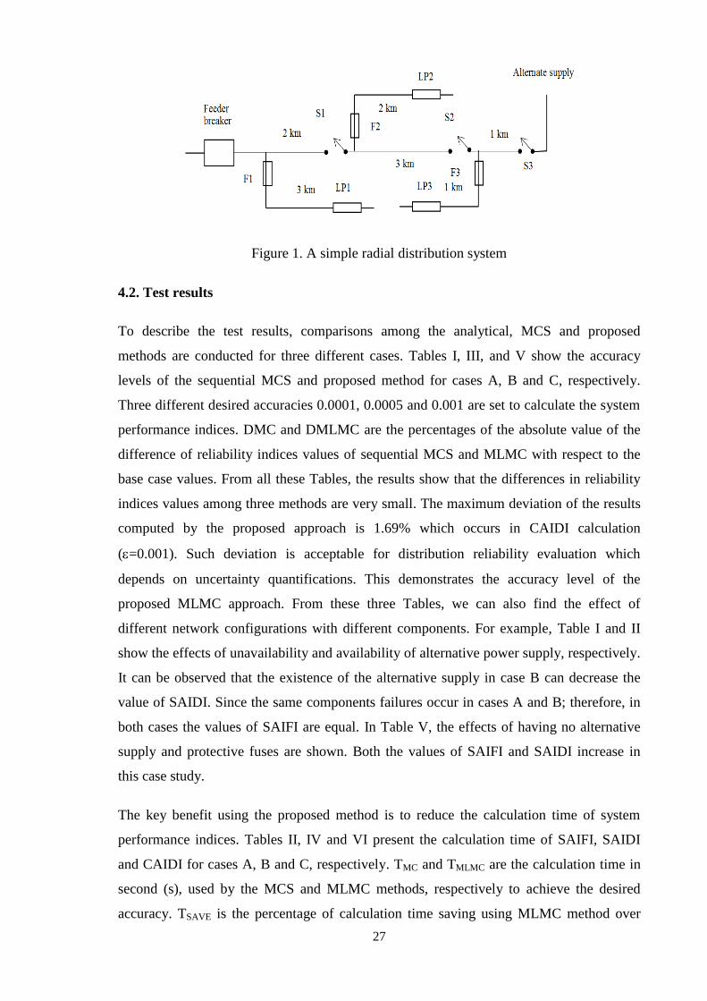
A simple radial distribution system [47] as shown in Figure 1 is chosen for case studies.

For simplicity, the feeder breaker and fuses are assumed as 100% reliable. Disconnect

switches S1 and S2 are normally closed and S3 is normally open. Average switching time

for switches S1, S2 and S3 are considered as 0.5, 0.5 and 1 hour, respectively. For the main

feeder and lateral section lines, the interruption rates are 0.1 and 0.25 interruptions/km/yr,

respectively and the average time to repair are 3 hours and 1 hour, respectively. There are

250, 100 and 50 customers at the load points LP1, LP2 and LP3, respectively. In order to

investigate the effect of different components on reliability assessment performance, three

cases of different configurations are considered.

1. Case A: alternate power supply is unavailable.

2. Case B: alternate supply is available.

3. Case C: both alternate power supply and lateral fuses are unavailable.

The drift and volatility values for both failure and repair processes are assumed as µ = 0.01

and σ = 0.4, respectively. These values are generally determined by using a time series of

TTF and TTR values [34]. These time series data are not currently available. Therefore, the

values of drift and volatility are determined by adjusting based on the accuracy levels for

an index calculation and kept as constant for rest of the indices calculation. Using

analytical technique, the system performance indices; SAIFI, SAIDI and CAIDI can be

evaluated [47] which are considered as base case results.

Variance reduction technique is a process which is used to increase the precision of the

output random variable from the simulation. If the variance is high, then the precision will

be less ( will be higher) and confidence intervals for the output random variable will be

increased. Similarly, if the variance is reduced, then the precision will be higher ( will be

less) and confidence intervals for the output random variable will be smaller and the

simulation will be more efficient. In this study, =0.0001, 0.0005 and 0.001 are predefined

as test accuracy to check the simulation efficiency at different accuracy levels. The

methodology was implemented using MATLAB and all computations were performed

using an Intel Core i7-4790 3.60-GHz processor.

27

Figure 1. A simple radial distribution system

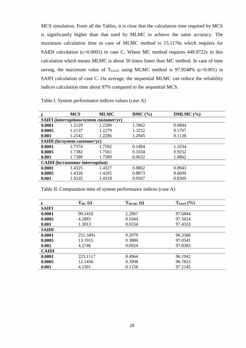
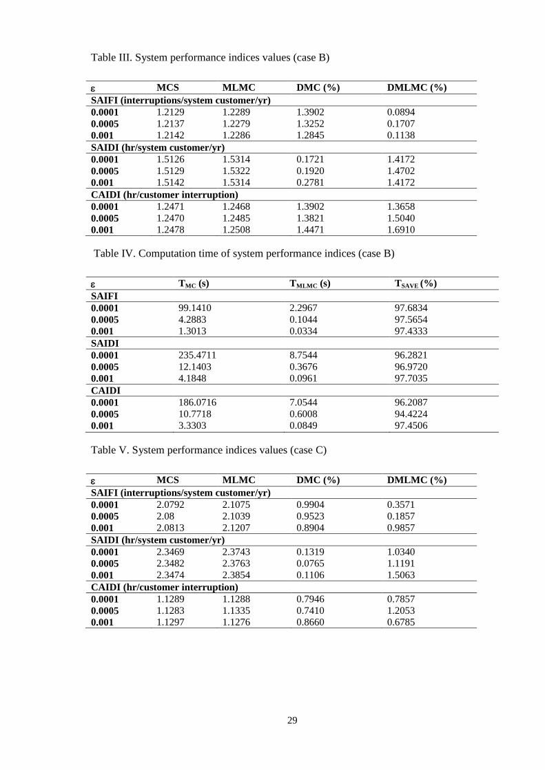
4.2. Test results

To describe the test results, comparisons among the analytical, MCS and proposed

methods are conducted for three different cases. Tables I, III, and V show the accuracy

levels of the sequential MCS and proposed method for cases A, B and C, respectively.

Three different desired accuracies 0.0001, 0.0005 and 0.001 are set to calculate the system

performance indices. DMC and DMLMC are the percentages of the absolute value of the

difference of reliability indices values of sequential MCS and MLMC with respect to the

base case values. From all these Tables, the results show that the differences in reliability

indices values among three methods are very small. The maximum deviation of the results

computed by the proposed approach is 1.69% which occurs in CAIDI calculation

(=0.001). Such deviation is acceptable for distribution reliability evaluation which

depends on uncertainty quantifications. This demonstrates the accuracy level of the

proposed MLMC approach. From these three Tables, we can also find the effect of

different network configurations with different components. For example, Table I and II

show the effects of unavailability and availability of alternative power supply, respectively.

It can be observed that the existence of the alternative supply in case B can decrease the

value of SAIDI. Since the same components failures occur in cases A and B; therefore, in

both cases the values of SAIFI are equal. In Table V, the effects of having no alternative

supply and protective fuses are shown. Both the values of SAIFI and SAIDI increase in

this case study.

The key benefit using the proposed method is to reduce the calculation time of system

performance indices. Tables II, IV and VI present the calculation time of SAIFI, SAIDI

and CAIDI for cases A, B and C, respectively. TMC and TMLMC are the calculation time in

second (s), used by the MCS and MLMC methods, respectively to achieve the desired

accuracy. TSAVE is the percentage of calculation time saving using MLMC method over

28

MCS simulation. From all the Tables, it is clear that the calculation time required by MCS

is significantly higher than that used by MLMC to achieve the same accuracy. The

maximum calculation time in case of MLMC method is 15.1176s which requires for

SAIDI calculation (=0.0001) in case C. Where MC method requires 448.9722s in this

calculation which means MLMC is about 30 times faster than MC method. In case of time

saving, the maximum value of TSAVE using MLMC method is 97.9548% (=0.001) in

SAIFI calculation of case C. On average, the sequential MLMC can reduce the reliability

indices calculation time about 97% compared to the sequential MCS.

Table I. System performance indices values (case A)

MCS MLMC DMC (%) DMLMC (%)

SAIFI (interruptions/system customer/yr)

0.0001 1.2129 1.2289 1.3902 0.0894

0.0005 1.2137 1.2279 1.3252 0.1707

0.001 1.2142 1.2286 1.2845 0.1138

SAIDI (hr/system customer/yr)

0.0001 1.7374 1.7592 0.1494 1.1034

0.0005 1.7382 1.7561 0.1034 0.9252

0.001 1.7389 1.7589 0.0632 1.0862

CAIDI (hr/customer interruption)

0.0001 1.4325 1.4327 0.8802 0.8943

0.0005 1.4326 1.4295 0.8873 0.6690

0.001 1.4335 1.4318 0.9507 0.8309

Table II. Computation time of system performance indices (case A)

TMC (s) TMLMC (s) TSAVE (%)

SAIFI

0.0001 99.1410 2.2967 97.6844

0.0005 4.2883 0.1044 97.5654

0.001 1.3013 0.0334 97.4333

SAIDI

0.0001 251.3491 9.2079 96.3366

0.0005 13.1915 0.3886 97.0541

0.001 4.2746 0.0924 97.8383

CAIDI

0.0001 223.1117 8.4964 96.1942

0.0005 12.1456 0.3908 96.7823

0.001 4.1501 0.1156 97.2145

29

Table III. System performance indices values (case B)



0.0001 1.2129 1.2289 1.3902 0.0894

0.0005 1.2137 1.2279 1.3252 0.1707

0.001 1.2142 1.2286 1.2845 0.1138


0.0001 1.5126 1.5314 0.1721 1.4172

0.0005 1.5129 1.5322 0.1920 1.4702

0.001 1.5142 1.5314 0.2781 1.4172


0.0001 1.2471 1.2468 1.3902 1.3658

0.0005 1.2470 1.2485 1.3821 1.5040

0.001 1.2478 1.2508 1.4471 1.6910

Table IV. Computation time of system performance indices (case B)


SAIFI

0.0001 99.1410 2.2967 97.6834

0.0005 4.2883 0.1044 97.5654

0.001 1.3013 0.0334 97.4333

SAIDI

0.0001 235.4711 8.7544 96.2821

0.0005 12.1403 0.3676 96.9720

0.001 4.1848 0.0961 97.7035

CAIDI

0.0001 186.0716 7.0544 96.2087

0.0005 10.7718 0.6008 94.4224

0.001 3.3303 0.0849 97.4506

Table V. System performance indices values (case C)



0.0001 2.0792 2.1075 0.9904 0.3571

0.0005 2.08 2.1039 0.9523 0.1857

0.001 2.0813 2.1207 0.8904 0.9857


0.0001 2.3469 2.3743 0.1319 1.0340

0.0005 2.3482 2.3763 0.0765 1.1191

0.001 2.3474 2.3854 0.1106 1.5063


0.0001 1.1289 1.1288 0.7946 0.7857

0.0005 1.1283 1.1335 0.7410 1.2053

0.001 1.1297 1.1276 0.8660 0.6785

30

Table VI. Computation time of system performance indices (case C)


SAIFI

0.0001 287.8317 7.1235 97.5251

0.0005 13.5947 0.3008 97.7873

0.001 4.0143 0.0821 97.9548

SAIDI

0.0001 448.9722 15.1176 96.6328

0.0005 24.1706 0.6412 97.3471

0.001 7.4004 0.1736 97.6541

CAIDI

0.0001 154.2683 5.9225 96.1609

0.0005 10.8705 0.2683 97.5318

0.001 3.2587 0.1035 96.8238

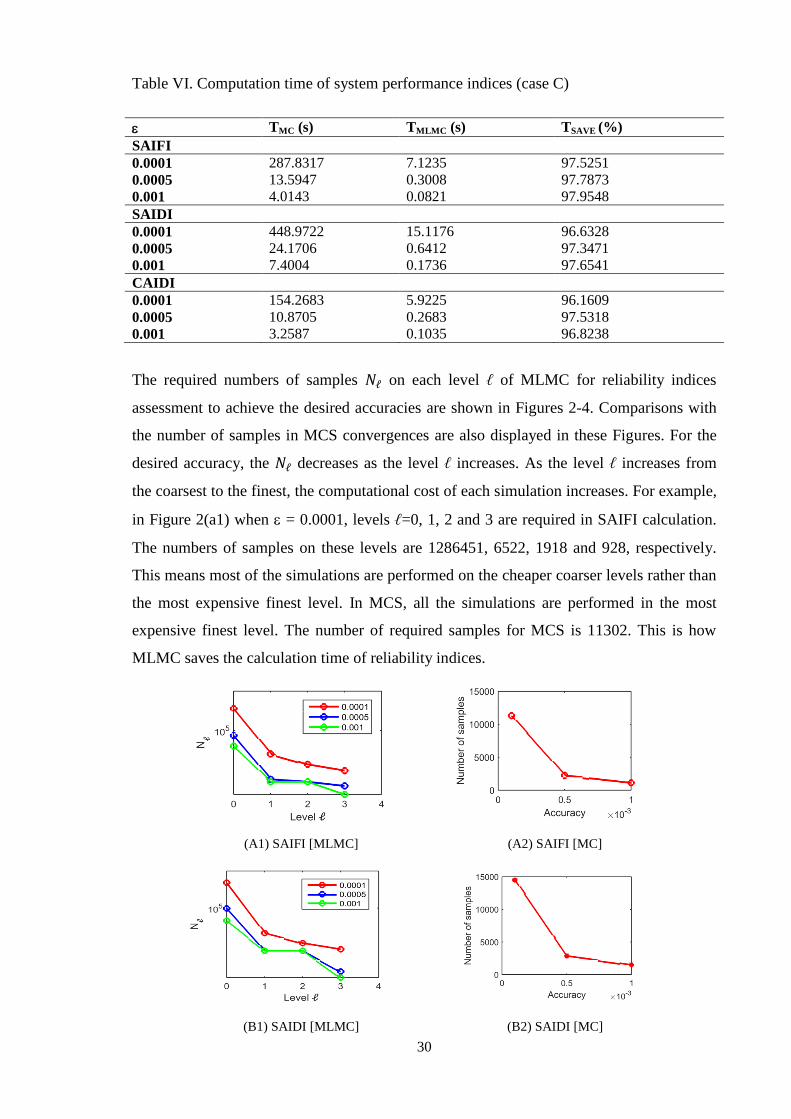
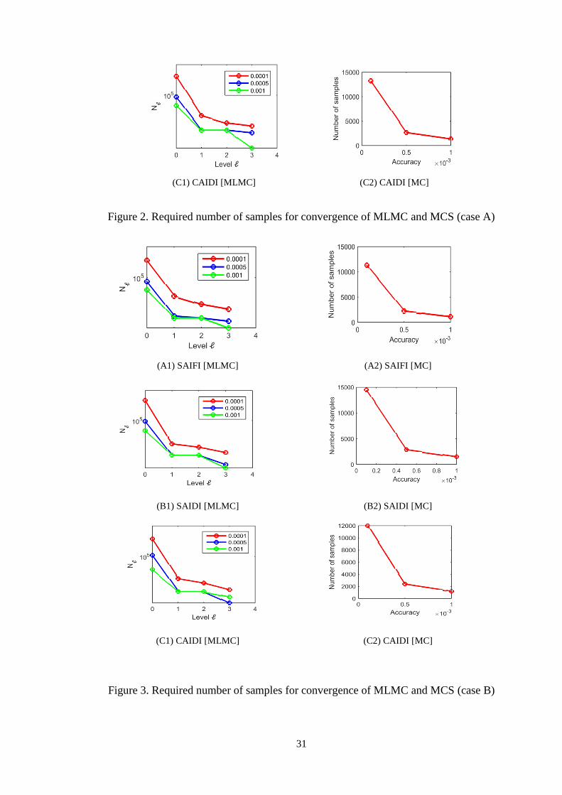
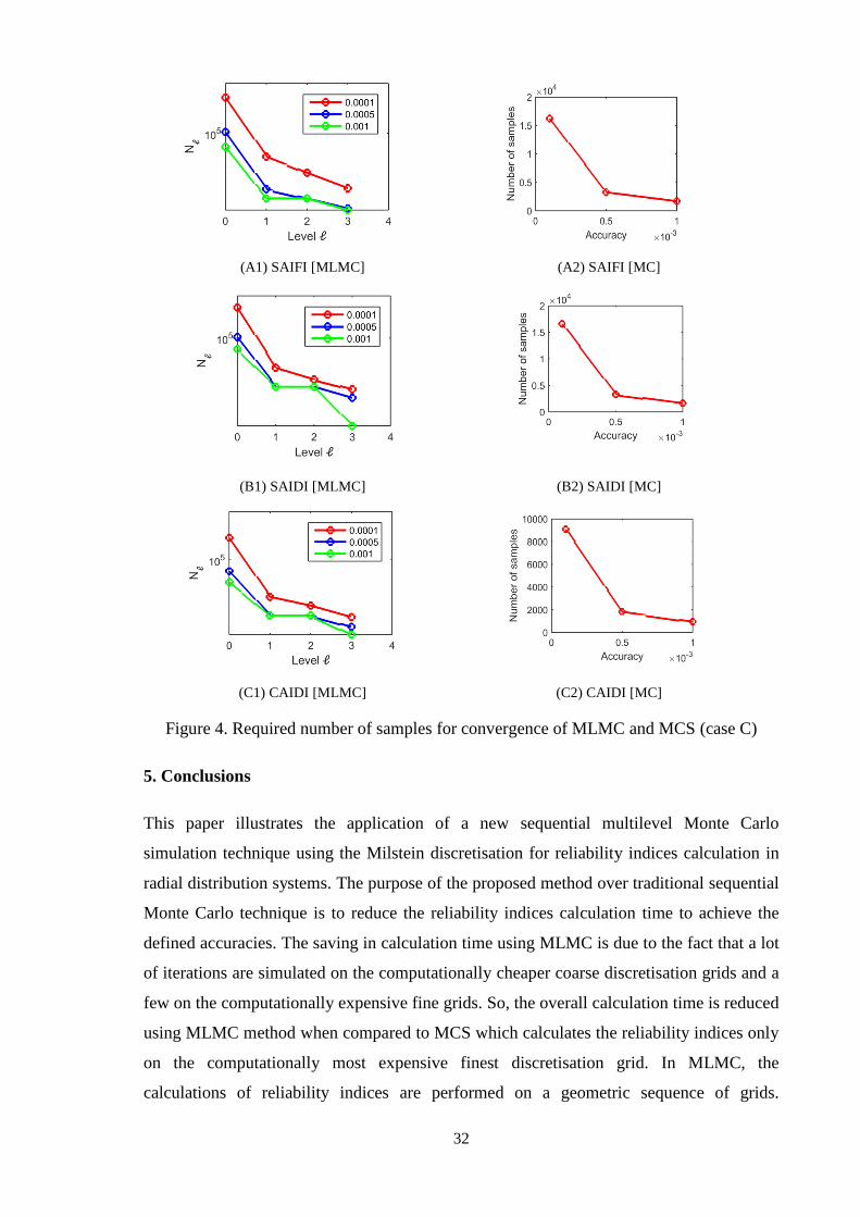
The required numbers of samples on each level of MLMC for reliability indices

assessment to achieve the desired accuracies are shown in Figures 2-4. Comparisons with

the number of samples in MCS convergences are also displayed in these Figures. For the

desired accuracy, the decreases as the level increases. As the level increases from

the coarsest to the finest, the computational cost of each simulation increases. For example,

in Figure 2(a1) when = 0.0001, levels =0, 1, 2 and 3 are required in SAIFI calculation.

The numbers of samples on these levels are 1286451, 6522, 1918 and 928, respectively.

This means most of the simulations are performed on the cheaper coarser levels rather than

the most expensive finest level. In MCS, all the simulations are performed in the most

expensive finest level. The number of required samples for MCS is 11302. This is how

MLMC saves the calculation time of reliability indices.

(A1) SAIFI [MLMC]

(A2) SAIFI [MC]

(B1) SAIDI [MLMC] (B2) SAIDI [MC]

31

(C1) CAIDI [MLMC] (C2) CAIDI [MC]

Figure 2. Required number of samples for convergence of MLMC and MCS (case A)

(A1) SAIFI [MLMC]

(A2) SAIFI [MC]

(B1) SAIDI [MLMC]

(B2) SAIDI [MC]


Figure 3. Required number of samples for convergence of MLMC and MCS (case B)

32

(A1) SAIFI [MLMC]

(A2) SAIFI [MC]

(B1) SAIDI [MLMC]

(B2) SAIDI [MC]


Figure 4. Required number of samples for convergence of MLMC and MCS (case C)

5. Conclusions

This paper illustrates the application of a new sequential multilevel Monte Carlo

simulation technique using the Milstein discretisation for reliability indices calculation in

radial distribution systems. The purpose of the proposed method over traditional sequential

Monte Carlo technique is to reduce the reliability indices calculation time to achieve the

defined accuracies. The saving in calculation time using MLMC is due to the fact that a lot

of iterations are simulated on the computationally cheaper coarse discretisation grids and a

few on the computationally expensive fine grids. So, the overall calculation time is reduced

using MLMC method when compared to MCS which calculates the reliability indices only

on the computationally most expensive finest discretisation grid. In MLMC, the

calculations of reliability indices are performed on a geometric sequence of grids.

33

Therefore, the less accurate approximation on the coarsest grid is sequentially corrected by

the estimators on the following finer grids. Thus, the finest grid accuracy is achieved by

MLMC method.

Two basic random variables time-to-failure and time-to-repair of each component are

modelled by jointly using stochastic differential equations and exponential probability

distributions. The impacts of different system configurations with various components on

three system performance indices (SAIFI, SAIDI and CAIDI) are discussed in this paper.

Comparisons between the proposed approach and analytical method demonstrated the

practicability of the method in a small scale distribution system. The differences in

reliability indices calculated data using MLMC are within 1.5% of values using an

analytical approach. In order to test the improvement in reliability indices calculation

efficiency, the results of the proposed approach are compared to the MCS method. The

results show that the proposed method can save the calculation time up to 97.95%

compared to sequential MCS. In the future, the proposed MLMC method will be tested on

the large distribution network. A method for probability distributions of these indices will

be presented in the future paper.

6. List of symbols and abbreviations

An average failure rate for a component j connected to load point i (given)

An average repair time for a component j connected to load point i (given)

An expected value of a random variable

Average failure rate for

Average failure rate for a component j connected to (simulated)

Average unavailability for a component j connected to (simulated)

Average unavailability for

Artificial operating histories

Artificial restoration histories

Brownian increments

Brownian motion

TMC Calculation time in second (s) used by MCS method

TMLMC Calculation time in second (s) used by MLMC method

CAIDI Customer average interruption duration index

Desired accuracy

µ Drift value

Estimation of expectation

Each grid level

L Highest grid level

ith sample of

34

Initial number of samples on each level

Load point i

MSE Mean square error

MC Monte Carlo

Monte Carlo estimator

MCS Monte Carlo simulation

MLMC Multilevel Monte Carlo

Number of customers at

Number of load points in the distribution system

Number of Monte Carlo samples

N Number of samples for MLMC convergence tests

Ns Number of samples Ns at levels which are determined using

Number of times component j failures during entire simulation period

DMC Percentage of the absolute value of the difference of reliability indices values

of sequential MCS with respect to the base case values

DMLMC Percentage of the absolute value of the difference of reliability indices values

of sequential MLMC with respect to the base case values

TSAVE Percentage of calculation time saving using MLMC method over MCS

simulation

SAIDI System average interruption duration index

SAIFI System average interruption frequency index

SDE stochastic differential equations

TTF Time-to-failure

TTR Time-to-repair

Total number of components fails that affect the service of

Total number of customers served

Random variable (system index in this study)

Estimated variance

σ Volatility value

References

1. Billinton R, Billinton JE. Distribution system reliability indices. IEEE Transactions on

Power Delivery 1989; 4: .

2. Kavousi-Fard A, Akbari-Zadeh MR. Reliability enhancement using optimal

distribution feeder reconfiguration. Neurocomputing 2013; 106: 1-11.

3. Park GP, Yoon YT. Application of ordinal optimization on reliability centered

maintenance of distribution system. European Transactions on Electrical Power 2012;

22: 391-401.

4. Allan R. Reliability evaluation of power systems; Springer, 2013.

35

5. Sankarakrishnan A, Billinton R. Sequential Monte Carlo simulation for composite

power system reliability analysis with time varying loads. IEEE Transactions on Power

Systems 1995; 10: 1540-1545.

6. Billinton R, Chen H, Ghajar R. A sequential simulation technique for adequacy

evaluation of generating systems including wind energy. IEEE Transactions on Energy

Conversion 1996; 11: 728-734.

7. Billinton R, Fotuhi-Firuzabad M, Bertling L. Bibliography on the application of

probability methods in power system reliability evaluation 1996-1999. IEEE

Transactions on Power Systems 2001; 16: 595-602.

8. Wang P, Billinton R. Time sequential distribution system reliability worth analysis

considering time varying load and cost models. IEEE Transactions on Power Delivery

1999; 14: 1046-1051.

9. Wang P, Billinton R. Reliability cost/worth assessment of distribution systems

incorporating time-varying weather conditions and restoration resources. IEEE

Transactions on Power Delivery 2002; 17: 260-265.

10. Hegazy Y, Salama M, Chikhani A. Adequacy assessment of distributed generation

systems using Monte Carlo simulation. IEEE Transactions on Power Systems 2003; 18:

48-52.

11. Silva AM, Cassula AM, Nascimento LC, Freire Jr JC, Sacramento CE, Guimarães

ACR. Chronological Monte Carlo-based assessment of distribution system reliability.

International Conference on Probabilistic Methods Applied to Power Systems, 2006; 1-

7.

12. Alvehag K, Söder L. A reliability model for distribution systems incorporating seasonal

variations in severe weather. IEEE Transactions on Power Delivery 2011; 26: 910-919.

13. Celli G, Ghiani E, Pilo F, Soma GG. Reliability assessment in smart distribution

networks. Electric Power Systems Research 2013; 104: 164-175.

14. Xudong W, Ling Q. Reliability evaluation for the distribution system with distributed

generation. European Transactions on Electrical Power 2011; 21: 895-909.

15. González-Fernández RA, da Silva AML. Reliability assessment of time-dependent

systems via sequential cross-entropy Monte Carlo simulation. IEEE Transactions on

Power Systems 2011; 26:2381-2389.

36

16. Li F. A fast approach of Monte Carlo simulation based on linear contribution factors to

distribution reliability indices. IEEE PES Transmission and Distribution Conference

and Exposition, 2003;973-977.

17. Zhaohong B, Xifan W. Studies on variance reduction technique of Monte Carlo

simulation in composite system reliability evaluation. Electric Power Systems Research

2002; 63: 59-64.

18. Naess A, Leira B, Batsevych O. System reliability analysis by enhanced Monte Carlo

simulation. Structural Safety 2009;31: 349-355.

19. Hou K, Jia H, Xu X, Liu Z, Jiang Y. A continuous time Markov chain based sequential

analytical approach for composite power system reliability assessment. IEEE

Transactions on Power Systems 2016;31:738-748.

20. Oliveira GC, Pereira MV, Cunha SH. A technique for reducing computational effort in

Monte-Carlo based composite reliability evaluation. IEEE Transactions on Power

Systems 1989;4:1309-1315.

21. Miranda V, de Magalhaes Carvalho L, da Rosa MA, da Silva AML, Singh C.

Improving power system reliability calculation efficiency with EPSO variants. IEEE

Transactions on Power Systems 2009;24:1772-1779.

22. Heinrich S. Multilevel monte carlo methods. in Large-scale scientific computing; edn,

Springer, 2001; 58-67.

23. Brandt A, Ilyin V. Multilevel Monte Carlo methods for studying large scale

phenomena in fluids. Journal of Molecular Liquids 2003; 105: 245-248.

24. Giles MB. Multilevel monte carlo path simulation. Operations Research 2008; 56: 607-

617.

25. Dereich S, Heidenreich F. A multilevel Monte Carlo algorithm for Lévy-driven

stochastic differential equations. Stochastic Processes and their Applications 2011;

121: 1565-1587.

26. Kloeden PE, Neuenkirch A, Pavani R. Multilevel Monte Carlo for stochastic

differential equations with additive fractional noise. Annals of Operations Research

2011; 189: 255-276.

27. Cliffe K, Giles MB, Scheichl R, Teckentrup AL. Multilevel Monte Carlo methods and

applications to elliptic PDEs with random coefficients. Computing and Visualization in

Science 2011; 14: 3-15.

37

28. Sanchez-Linares C, de la Asunción M, Castro M, Mishra S, Šukys J. Multi-level Monte

Carlo finite volume method for shallow water equations with uncertain parameters

applied to landslides-generated tsunamis. Applied Mathematical Modelling 2015; 39:

7211-7226.

29. Lu D, Zhang G, Webster C, Barbier C. Multilevel Monte Carlo method with

application to uncertainty quantification in reservoir simulation, AGU Fall Meeting

Abstracts, 2014; 3692.

30. Retterath B, Chowdhury AA, Venkata SS. Decoupled substation reliability assessment.

International Journal of Electrical Power & Energy Systems 2005; 27: 662-668.

31. Retterath B, Venkata S, Chowdhury AA. Impact of time-varying failure rates on

distribution reliability. International Journal of Electrical Power & Energy Systems

2005; 27: 682-688.

32. Moradkhani A, Haghifam MR, Mohammadzadeh M. Failure rate estimation of

overhead electric distribution lines considering data deficiency and population

variability. International Transactions on Electrical Energy Systems 2015; 25: 1452-

1465.

33. Chowdhury A, Koval D. Power distribution system reliability: practical methods and

applications; John Wiley & Sons: New Jersey, 2011.

34. Wang K, Crow ML. Fokker-Planck equation application to analysis of a simplified

wind turbine model. North American Power Symposium, 2012; 1-5.

35. Zárate-Miñano R, Milano F. Construction of SDE-based wind speed models with

exponentially decaying autocorrelation. Renewable Energy 2016; 94: 186-196.

36. Kalos MH, Whitlock PA. Monte carlo methods: John Wiley & Sons, 2008.

37. Elfverson D, Hellman F, Målqvist A. A multilevel Monte Carlo method for computing

failure probabilities. arXiv preprint arXiv:1408.6856, 2014.

38. Giles M. Improved multilevel Monte Carlo convergence using the Milstein scheme. in

Monte Carlo and quasi-Monte Carlo methods 2006; ed: Springer, 2008; 343-358.

39. Harrison JM. Brownian motion and stochastic flow systems; Wiley: New York, 1985.

40. Oksendal B. Stochastic differential equations: an introduction with applications;

Springer, 2013.

38

41. Giles MB. Multilevel Monte Carlo for basket options. Proceedings of the 2009 Winter

Simulation Conference, 2009; 1283-1290.

42. Kloeden PE, Platen E. Higher-order implicit strong numerical schemes for stochastic

differential equations. Journal of statistical physics 1992; 66: 283-314.

43. Billinton R, Allan RN. Reliability evaluation of engineering systems; Springer, 1992.

44. Billinton R, Wang P. Teaching distribution system reliability evaluation using Monte

Carlo simulation. IEEE Transactions on Power Systems 1999; 14: 397-403.

45. Goel L, Billinton R. Evaluation of interrupted energy assessment rates in distribution

systems. IEEE Transactions on Power Delivery 1991; 6:1876-1882.

46. Sultana B, Sultana U, Bhatti AR. Review on reliability improvement and power loss

reduction in distribution system via network reconfiguration. Renewable and

Sustainable Energy Reviews 2016;66:297-310.

47. Billinton R, Li W. Distribution system and station adequacy assessment. in Reliability

assessment of electric power systems using Monte Carlo methods; ed: Springer, 1994;

209-254.

39

Chapter 3

Comparative Reliability Study of Euler-Maruyama and

Milstein Scheme Based Methods

40


Title of Paper Accelerated distribution systems reliability evaluation by multilevel Monte Carlo simulation:

Implementation of two discretisation schemes





manuscript style

Publication Details A. S. Nazmul Huda and Rastko Živanović (2017) Accelerated distribution systems reliability

evaluation by multilevel Monte Carlo simulation: Implementation of two discretisation schemes,

IET Generation, Transmission & Distribution, 11(13), 3397-3405.

Link: https://ieeexplore.ieee.org/document/8063034/

Principal author


(Candidate)

A. S. Nazmul Huda


Developed reliability evaluation model, performed simulation and numerical analysis, prepared

manuscript.





paper.

Signature

Date 07.09.2018








Signature

Date 13.08.2018

https://ieeexplore.ieee.org/document/8063034/

41

Accelerated distribution systems reliability evaluation by multilevel Monte Carlo

simulation: Implementation of two discretisation schemes

Abstract- This article presents the performances of two discretisation schemes which are

implemented in a novel multilevel Monte Carlo (MLMC) method for reliability calculation

of power distribution systems. The motivation of using the proposed approach is to reduce

the computational effort of standard Monte Carlo simulation (MCS) and accelerate the

overall distribution system reliability evaluation process. The MLMC methods are

implemented through solving the stochastic differential equations (SDE) of random

variables related to the reliability indices. The SDE can be solved using different

discretisation schemes. Two different discretisation schemes namely, Euler-Maruyama and

Milstein are utilised in this paper. For this reason, the proposed MLMC methods are named

as Euler-Maruyama MLMC (EM-MLMC) and Milstein MLMC (M-MLMC). The

reliability evaluation efficiency of the methods is analysed and compared based on

accuracy and computational time saving for basic reliability assessment of Roy Billinton

Test System (RBTS). Numerical results show that both methods reduce the computational

time required to estimate the reliability indices compared to the same discretisation

schemes used in MCS and maintain satisfactory accuracy levels.

Keywords—multilevel Monte Carlo (MLMC); computational complexity; distribution

system; reliability; discretisation schemes

1. Introduction

In power distribution systems planning, reliability analysis is an essential step for

supplying the electricity with minimum customers’ interruptions and cost. Reliability is

generally measured by few indices related to the frequency and duration of the

interruptions [1]. Component failure rate and unavailability are the fundamental reliability

indices to measure the load point (LP), feeder as well as overall distribution system

reliability. Failure rate and unavailability indices measure the expected number of failures

and their duration for individual customers, respectively. Some reliability indices measure

the feeder as well as overall system interruption frequency and duration related

information. For example, System Average Interruption Frequency Index (SAIFI) and

Customer Average Interruption Duration Index (CAIDI) calculate the average number of

sustained interruptions that customers would experience in a year and average duration of

each interruption, respectively. Two other common indices- System Average Interruption

42

Duration Index (SAIDI) and Expected Energy Not Supplied (EENS) measure the average

interruption duration for each customer in a year and total amount of energy interruption in

a year, respectively [2, 3].

The number of outages associated with a LP of a feeder and their restoration times vary

randomly with time [4]. As a result, the values of reliability indices of the distribution

systems also vary randomly. Approximations of reliability indices by considering the

variability of the indices provide more accurate prediction of distribution systems

performance. Commonly used approaches for reliability evaluation are analytical and

Monte Carlo simulation (MCS) methods [5, 6]. Analytical approach evaluates the expected

average value of a particular index without considering the variability of the index. On the

other hand, MCS technique estimates the indices by simulating the components random

failure and restoration behaviours over a time period. Therefore, MCS approach is

extensively used in reliability evaluation applications. However, the main constraint of

MCS is that its computational burden increases rapidly with the increased accuracy level

for highly reliable systems. The presence of increased number of time-dependent random

variables and system configurations complexities also greatly increase the computation

time of reliability assessment. This motivates the development of a new technique which

can reduce the computational effort of MCS in order to achieve the target convergence

criteria without compromising the accuracy levels of the indices.

Several methods have been proposed to improve the computational efficiency of crude

MCS in power system applications [7-10]. However, there is a lack of research to improve

the computational efficiency of MCS applications in distribution system reliability

evaluation by employing advanced MCS methods. Therefore, in this paper, we propose a

novel multilevel Monte Carlo (MLMC) simulation technique that incorporates the idea of

control variates in distribution systems reliability evaluation.

The MLMC method is an advanced MCS technique which has been recently developed for

the estimation of expectations by constructing the stochastic differential equations (SDE)

[11] of system random variables. In standard MCS method, all the samples are simulated

on a single finest grid level at the highest accuracy and computational cost. On the other

hand, proposed MLMC method uses a hierarchy of discretisation levels and simulations

are carried out on multiple different grid levels, starting from the coarsest grid level. The

simulation accuracy and computational burden using coarse levels are less than the

simulation using fine levels. By using information on multiple levels, MLMC method

43

needs few samples on the expensive fine levels to achieve the target convergence criteria

and thus the overall computational cost is dramatically reduced than MCS. The MLMC

based methods are implemented by solving the SDE using different discretisation schemes.

In this study, we propose Euler-Maruyama discretisation (EMD) and Milstein

discretisation (MD) schemes for the approximations of the numerical solution of SDE. In

our previous studies [12, 13], we have shown the effectiveness of the MLMC method on a

simple distribution network. In this study, the proposed method is tested on three

benchmark large and complex distribution networks.

In Section 2, we describe the basics of MLMC and its convergence criteria. In Section 3,

we present the proposed methodology of the distribution system reliability evaluation. In

this Section, firstly we develop the SDE modelling of component average time-to-failure

and time-to-repair variables based on the proposed two discretisation schemes. The SDE

models of LP, feeder and overall system reliability indices are constructed using these

variables. Reliability indices SAIFI, SAIDI, CAIDI and EENS are considered for

evaluation. In Section 4, we describe the test networks and numerical results. Simulation

accuracy and running time are used to illustrate the effectiveness of the proposed methods.

The results from the proposed methods are compared with the standard MCS and

analytical techniques. Finally, Section 5 concludes the article.

2. Multilevel Monte Carlo simulation

2.1. Principles of MLMC

Suppose we want to estimate . Let be the approximation of . R is the target

reliability index and is a function of simulated random variables. In MCS method, an

average value of , is approximated by using a large number of simulations on a

single fine grid level [14]. According to the MCS method, unbiased estimator for

can be expressed as follows:

(1)

where

is the ith sample of and is the total number of required samples on the

finest grid level. The uncertainty around the approximation is measured by the variance of

the estimator. The variance of this estimator is and the root mean square error

(RMSE) is . Mathematically, is introduced as big O notation, which is used to

describe the complexity of a function by omitting constant factors and lower order terms.

44

Here, we simply express the relationship between the number of Monte Carlo samples and

accuracy level using big O notation [13]. The convergence criterion in MCS method is

based on the desired RMSE value. This RMSE value is often represented as simulation

accuracy. To achieve an accuracy of , it requires samples. This means for a

high reliable system with smaller , we need to simulate a large number of samples which

results in high computational burden. To reduce the computational burden, variance

reduction techniques are generally applied by maintaining the reasonable accuracy level.

For simplicity, standard MC method could be referred as single level MC simulation due to

the estimation of by on a single fine level . On the other hand, MLMC

method uses multiple grid levels, with (coarsest level) and

(finest level). is a nonnegative integer.

For two-level version of MLMC, we can estimate by simulating which

approximates . denotes the samples or approximations on the computationally

cheapest coarsest level . Therefore, the idea of two levels MLMC can be written by

the following way:

(2)

In the above Equation (2), each expectation on the single level is individually assessed by

the traditional MCS. Each level of the grid uses a different number of samples in a way

which reduces the overall variance for a given convergence criteria. Mathematically, the

general idea of MLMC for any number of grid levels can be formulated as follows:

(3)

Let be an unbiased MCS estimator for using samples for . Also, let

be the MCS estimator for using samples for . Then

we get

(4)

and

(5)

The overall estimator of MLMC method for each reliability index of distribution systems

can be expressed by combining the Equations (4) and (5) as follows:

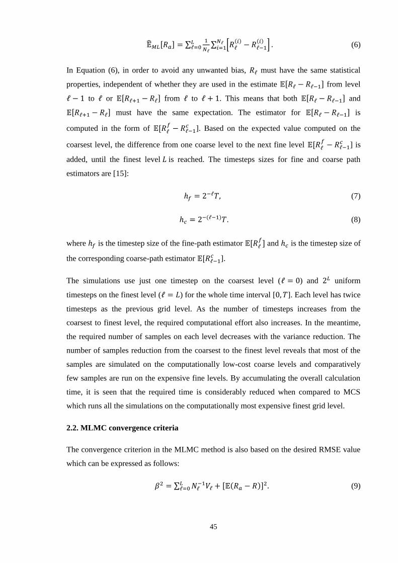
45

(6)

In Equation (6), in order to avoid any unwanted bias, must have the same statistical

properties, independent of whether they are used in the estimate from level

to or from to . This means that both and

must have the same expectation. The estimator for is

computed in the form of

]. Based on the expected value computed on the

coarsest level, the difference from one coarse level to the next fine level

] is

added, until the finest level is reached. The timesteps sizes for fine and coarse path

estimators are [15]:

(7)

. (8)

where is the timestep size of the fine-path estimator and is the timestep size of

the corresponding coarse-path estimator ].

The simulations use just one timestep on the coarsest level ( ) and uniform

timesteps on the finest level ( ) for the whole time interval [ ]. Each level has twice

timesteps as the previous grid level. As the number of timesteps increases from the

coarsest to finest level, the required computational effort also increases. In the meantime,

the required number of samples on each level decreases with the variance reduction. The

number of samples reduction from the coarsest to the finest level reveals that most of the

samples are simulated on the computationally low-cost coarse levels and comparatively

few samples are run on the expensive fine levels. By accumulating the overall calculation

time, it is seen that the required time is considerably reduced when compared to MCS

which runs all the simulations on the computationally most expensive finest grid level.

2.2. MLMC convergence criteria

The convergence criterion in the MLMC method is also based on the desired RMSE value

which can be expressed as follows:

(9)

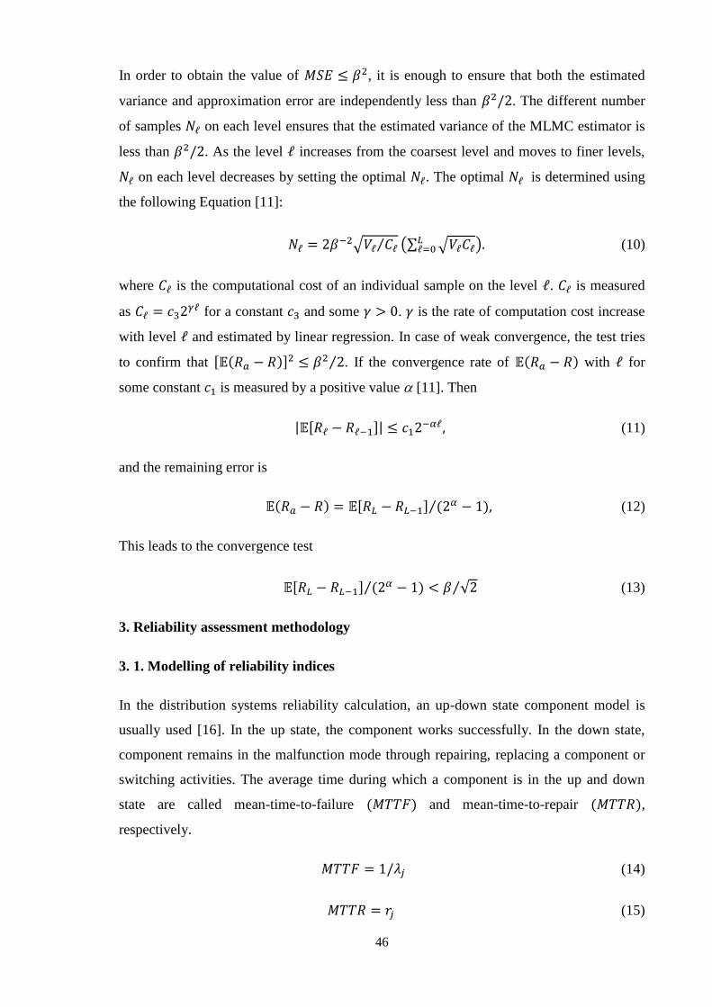
46

In order to obtain the value of , it is enough to ensure that both the estimated

variance and approximation error are independently less than . The different number

of samples on each level ensures that the estimated variance of the MLMC estimator is

less than . As the level increases from the coarsest level and moves to finer levels,

on each level decreases by setting the optimal . The optimal is determined using

the following Equation [11]:

(10)

where is the computational cost of an individual sample on the level . is measured

as for a constant and some . is the rate of computation cost increase

with level and estimated by linear regression. In case of weak convergence, the test tries

to confirm that . If the convergence rate of with for

some constant is measured by a positive value [11]. Then

(11)

and the remaining error is

(12)

This leads to the convergence test

(13)

3. Reliability assessment methodology

3. 1. Modelling of reliability indices

In the distribution systems reliability calculation, an up-down state component model is

usually used [16]. In the up state, the component works successfully. In the down state,

component remains in the malfunction mode through repairing, replacing a component or

switching activities. The average time during which a component is in the up and down

state are called mean-time-to-failure and mean-time-to-repair ,

respectively.

(14)

(15)

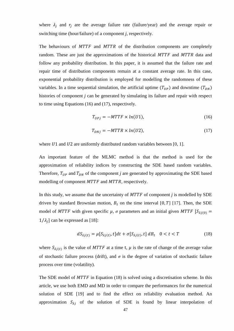
47

where and are the average failure rate (failure/year) and the average repair or

switching time (hour/failure) of a component j, respectively.

The behaviours of and of the distribution components are completely

random. These are just the approximations of the historical and data and

follow any probability distribution. In this paper, it is assumed that the failure rate and

repair time of distribution components remain at a constant average rate. In this case,

exponential probability distribution is employed for modelling the randomness of these

variables. In a time sequential simulation, the artificial uptime and downtime

histories of component j can be generated by simulating its failure and repair with respect

to time using Equations (16) and (17), respectively.

(16)

(17)

where and are uniformly distributed random variables between [0, 1].

An important feature of the MLMC method is that the method is used for the

approximation of reliability indices by constructing the SDE based random variables.

Therefore, and of the component j are generated by approximating the SDE based

modelling of component and , respectively.

In this study, we assume that the uncertainty of of component j is modelled by SDE

driven by standard Brownian motion, on the time interval [ ] [17]. Then, the SDE

model of with given specific µ, σ parameters and an initial given

can be expressed as [18]:

(18)

where is the value of at a time , µ is the rate of change of the average value

of stochastic failure process (drift), and σ is the degree of variation of stochastic failure

process over time (volatility).

The SDE model of in Equation (18) is solved using a discretisation scheme. In this

article, we use both EMD and MD in order to compare the performances for the numerical

solution of SDE [19] and to find the effect on reliability evaluation method. An

approximation of the solution of SDE is found by linear interpolation of

48

[20]. The EMD and MD with n timesteps, timestep size and

Brownian increments are expressed by [21]:

EMD:

(19)

and MD:

(20)

where with and with

. are independent and normally distributed random

variables.

Now Equation (16) can be rewritten as follows using SDE model of , :

(21)

Similarly, the SDE model of can be determined. The values of drift, µ and

volatility, σ are assumed same as for stochastic failure process. If is a constant for

component j and . Then initial for component j is . Like Equation

(21), can be determined via using Equation (17):

(22)

The values of average failure rate, and average unavailability, for a component j can

be calculated using the following expressions:

(23)

(24)

where is the number of times component j fails for entire simulation period and N is the

desired number of simulated periods. Now, average failure rate, and annual

unavailability, for LP i can be calculated as follows:

49

(25)

(26)

where is the number of components failures that affect the service of LP i. Using the

Equations (27) and (28), proposed reliability indices can be defined as follows:

(27)

(28)

(29)

(30)

where is the number of customers at LP i, is the total number of customers served.

On the other hand, is the number of LPs in the distribution system and is the

average load level at LP i.

3.2. MLMC simulation steps

The overall procedure for power distribution system reliability evaluation is briefly

summed up in the following steps:

(1) Distribution components reliability data are defined at first i.e. component average

failure rate and repair time. We also assume some MLMC simulation parameters as

follows:

a) Number of samples for convergence tests, N [6000]

b) Initial number of samples on each level , [500]

c) Desired accuracy, [0.001]

d) Drift value, µ [0.02] and

e) Volatility value, σ [0.6].

50

(2) The SDE model of is constructed using Equation (18) for a component of

average failure rate, .

(3) The SDE models of on levels and are solved by EMD and MD

schemes using Equations (19) and (20), respectively. For coarse and fine levels, the

solutions of SDE models are defined by Equations (31)-(34).

EMD:

(31)

(32)

MD:

(33)

(34)

(4) The following parameters are then computed on levels and using the

Equations (31)-(34) depending on discretisation scheme used.

(a) and histories for each component are generated using Equations (21) and (22),

respectively.

(b) The values of and for each component are calculated using Equations (23) and

(24), respectively.

(c) The values of and for each LP are calculated using Equations (25) and (26),

respectively.

(d) SAIFI, SAIDI, CAIDI and EENS are determined using Equations (27)-(30),

respectively.

(5) The sum of system performance indices values on levels and are

calculated using Equation (3). The whole process starting from step (2) is repeated until the

sample size is reached to is N.

51

(6) In order to achieve the target convergence criteria for each reliability index calculation

by Equation (9), initially, the number of grid levels for MLMC simulation is set at .

(7) Using an initial number of samples , the number of samples on each level

is determined. At the same time, the sum of system performance indices values

is updated on each level .

(8) The absolute value of average system performance index, and variance

are calculated on each level .

(9) The optimal number of samples on each level is determined using Equation (10).

The optimal is compared to the already calculated on that level. If is larger than

, then additional samples on each level are determined. In the same time, the mean

reliability index value and variance on each level are also updated. The purpose of

determining the optimal is to make the variance

less than .

(10) The weak convergence criteria of Equation (9) ensures that the approximation error is

less than . If remaining error is greater than , then a new level is

introduced. The whole process is repeated from step (7) until the target convergence

criterion is met.

(11) Finally, the overall multilevel estimator for each system performance index is

computed using Equation (6).

4. Case studies and numerical results

4.1. Test distribution networks

The Roy Billinton Test System (RBTS) is a 6 bus test system with five load buses (bus2-

bus6). In this paper, three distributions networks with three different buses (buses 3, 5 and

6) are considered as test networks [22]. Figs. 1a, 1b and 1c show the buses 3, 5 and 6 test

networks, respectively. RBTS bus 3 has 8 feeders and 42 LPs. RBTS bus 5 has 4 feeders

and 26 LPs. RBTS bus 6 has 4 feeders and 40 LPs. The purpose of using three different

networks is to find the effects on reliability computation by considering different networks

sizes and the number of SDE. The number of SDE model in a distribution system

reliability evacuation depends on the types of components varying their feeder length.

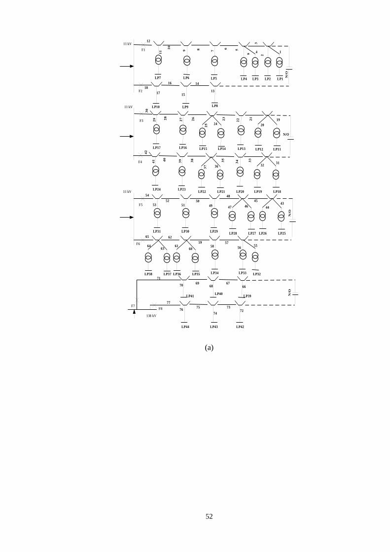
52

11 kV

N/O

F1

N/O

F2 13

LP7

LP31 LP30 LP29

LP34 LP33

11 kV

11 kV

138 kV

F3

F4

F5

F6

F7F8

LP2 LP1LP3LP4LP5LP6

LP8LP9LP10

LP11LP12LP13LP14LP15LP16LP17

LP18LP19LP20LP22LP24

LP26LP28

LP23LP21

LP25LP27

LP41

LP43

LP32

LP44 LP42

LP35LP36LP37LP38

LP39LP40

12

4 1

18

17

16 14

15

19

2024

313236

4344

45

4647

48

49

5051

5253

54

5556

5758

59

6061

6364

6265

6667

7273

74

7576

77

6869

70

71

(a)

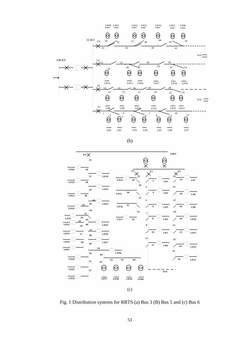
53

138 KV

11 KV

LP22 LP23 LP20

34

LP21 LP24 LP25 LP26

F4

33

35

36

37 38

39

4042

41

43

N/O

1110

25

12

F1

3

45 6

78 9

LP1 LP2 LP3 LP4 LP5 LP6 LP7

F212

13

14

LP14 LP15 LP16

23

2426

27

28 30 F3

N/O

LP9 LP10 LP11 LP8 LP12 LP13

15

16

17

18

19 21

20

22

LP18 LP19

31 32

LP17

29

(b)

22 LP11

2 LP1

4 LP2

6 LP3

8 LP4

10 LP5

12 LP6

LP18 36

LP20 38

LP22 40

LP24

LP31

LP32

LP33

LP34

LP35

LP28

LP29

LP30

37 LP19

LP21

LP23

LP25

47

LP26

LP27

LP36

LP14 28

LP17 34

30

32

27

29

31

33

1

3

5

7

9

11

13

15

17

19

21

23

25

35

39

LP37 LP38 LP39 LP40

42

41

43

44

53

54

55

56

57

58

50

51

52

59

60

6162 63 64

49

48

46

45

F2F1F3

F4

LP15

LP16

14 LP7

16 LP8

18 LP9

20 LP10

24 LP12

26 LP13

N/O

33KV

(c)

Fig. 1 Distribution systems for RBTS (a) Bus 3 (B) Bus 5 and (c) Bus 6

54

The network at bus 3 represents a typical industrial and large user network. The networks

at bus 5 and 6 represent urban and rural types, respectively. These networks have several

components between substation and LPs such as transmission lines, feeder breakers,

transformers, fuses and disconnector switches. The failure of any component causes an

outage of the LP(s). In this study, feeder breakers are assumed as 100% reliability. The

failures of main and lateral section lines are considered with the availability of

disconnectors, fuses, alternative supply and transformer. The alternative supply is used to

supply power to that section of the main feeder which becomes disconnected from the

main supply after the isolation of faulted section. Faults on a lateral distributor are

normally automatically cleared by a fuse and therefore, service on the main feeder is

maintained. The actions of transformers are restored by repairing. The reliability and

system data of the components can be found in [23]. The lengths of the primary and lateral

feeders, customers and loading data of the networks are taken from [22].

4.2. Numerical results

4.2.1. Calculation accuracy

The failure rate of a LP is affected by the numbers of components failures associated with

the LP and length of feeders. The failure rates of LP with long feeders are higher than

those with the short feeders. SAIFI value depends on the LPs failure rates and number of

customers served. For example, in Fig. 2(a), the value of SAIFI for feeder 1 (F1) is higher

than F2. For F1, each LP failure rate is affected by the failures of five main feeder sections,

one lateral section and transformer. The reduced value of SAIFI for F2 is due to the

reduced number of failures (three main feeder sections and one lateral section). The values

of SAIDI and CAIDI depend on the components failure rate, repair time and number of

customers served. In the current study, restoration of a component is performed either

repairing or switching action. The average repair time of a component is longer than the

switching time. The reduced values of SAIDI and CAIDI occur because of the fewer

components failure as well as components less unavailability time. Similarly, EENS values

vary with the components failure rates, repair times and average load level of the LPs.

In this section, we evaluate and compare the accuracy of different methods based on EMD

and MD schemes i.e. Euler-Maruyama MLMC (EM-MLMC), Milstein MLMC (M-

MLMC), Euler-Maruyama MC (EM-MC) and Milstein MC (M-MC) with respect to the

base analytical value. The reliability indices values for different feeders of the test

distribution networks are shown in Figs. 2, 3 and 4 [a, b, c and d]. From these Figs., it is

55

clear that the accuracy levels of the proposed methods are acceptable and very close to the

true values.

For the network RBTS bus-3, the maximum deviation of the results from the analytical

value computed by the proposed EM-MLMC and M-MLMC approaches are 2.9854% and

3.4102% which occur in the calculation of F7-SAIDI and F8-SAIDI, respectively. The

maximum deviation using EM-MLMC and M-MLMC approaches for RBTS Bus-5

network are 2.4894% and 4.0980%, respectively where both occur in the calculation of F2-

SAIFI. On the other hand, in the case of reliability indices calculation of RBTS bus-6

network, these deviations are 3.7399% and 4.0802%, whereas the indices F3-SAIFI and

F4-SAIFI are computed, respectively.

Tables 1, 2 and 3 present the performances of the proposed methods to evaluate the overall

system reliability indices. For the network RBTS bus-3, the maximum deviation of the

results computed by the proposed EM-MLMC and M-MLMC approaches are 5.2234% and

3.9354% respectively where both occur in the calculation of SAIFI. The maximum

deviation for RBTS bus-5 network using EM-MLMC and M-MLMC approaches are found

3.2339% and 2.2395% which occur in the calculation of SAIFI and CAIDI, respectively.

On the other hand, in the case of reliability indices calculation of RBTS bus-6 network,

these deviations are 2.0895% and 1.9853%, respectively where the index CAIDI is

computed.

The accuracy levels of the indices values are basically influenced by the associated

random variables and number of samples simulated on the grid levels. In MLMC methods,

both coarse and fine levels are required where most of the samples are simulated on the

coarse levels at low accuracy and relatively few samples are simulated on the fine levels at

high accuracy. On the other hand, in MC methods, all the simulations are run on the finest

level at the highest accuracy. Therefore, the accuracy levels of the indices computed by the

MCS are generally higher than the results from MLMC methods. For example, in M-

MLMC, levels =0, 1, 2 and 3 are required for CAIDI calculation. The numbers of samples

on these levels are 13001866, 67343, 27537 and 10320, respectively. This means that most

of the simulations are performed on the coarser levels rather than the finest level. In M-

MC, the number of required samples is 32032 and all the simulations are performed on the

finest level =3.

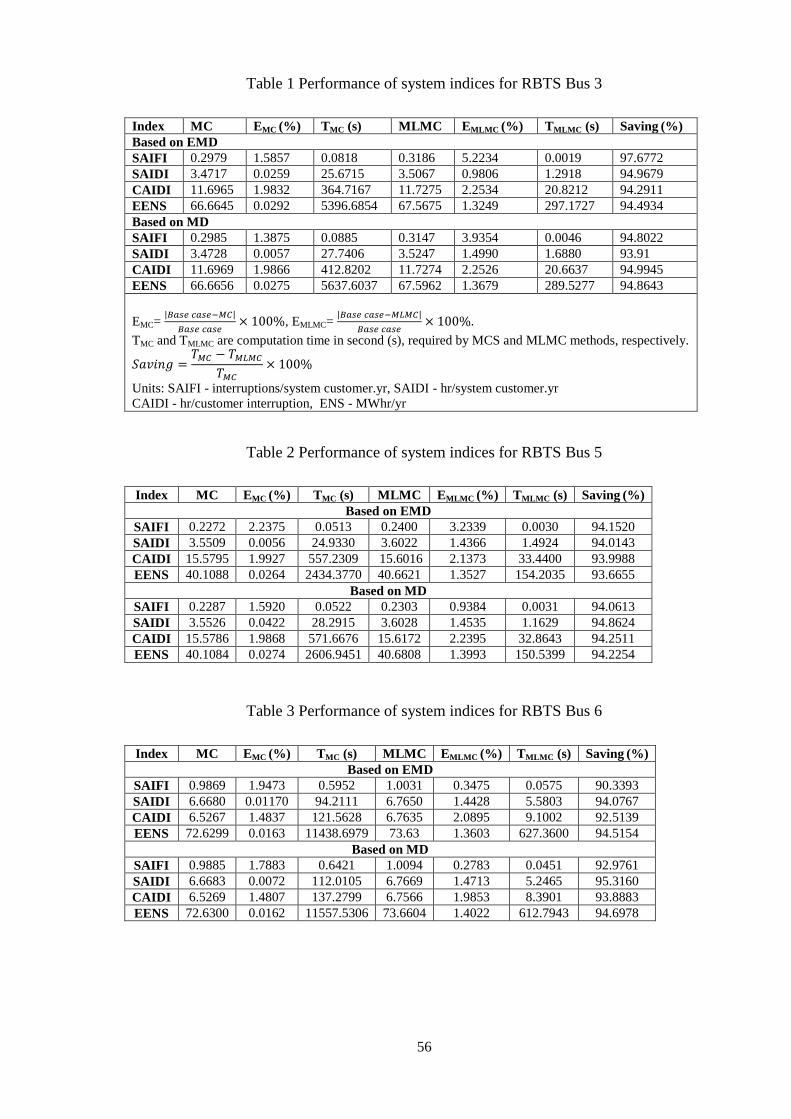
56

Table 1 Performance of system indices for RBTS Bus 3

Index MC EMC (%) TMC (s) MLMC EMLMC (%) TMLMC (s) Saving (%)

Based on EMD

SAIFI 0.2979 1.5857 0.0818 0.3186 5.2234 0.0019 97.6772

SAIDI 3.4717 0.0259 25.6715 3.5067 0.9806 1.2918 94.9679

CAIDI 11.6965 1.9832 364.7167 11.7275 2.2534 20.8212 94.2911

EENS 66.6645 0.0292 5396.6854 67.5675 1.3249 297.1727 94.4934

Based on MD

SAIFI 0.2985 1.3875 0.0885 0.3147 3.9354 0.0046 94.8022

SAIDI 3.4728 0.0057 27.7406 3.5247 1.4990 1.6880 93.91

CAIDI 11.6969 1.9866 412.8202 11.7274 2.2526 20.6637 94.9945

EENS 66.6656 0.0275 5637.6037 67.5962 1.3679 289.5277 94.8643

EMC=

, EMLMC=

TMC and TMLMC are computation time in second (s), required by MCS and MLMC methods, respectively.

Units: SAIFI - interruptions/system customer.yr, SAIDI - hr/system customer.yr

CAIDI - hr/customer interruption, ENS - MWhr/yr



Based on EMD

SAIFI 0.2272 2.2375 0.0513 0.2400 3.2339 0.0030 94.1520

SAIDI 3.5509 0.0056 24.9330 3.6022 1.4366 1.4924 94.0143

CAIDI 15.5795 1.9927 557.2309 15.6016 2.1373 33.4400 93.9988

EENS 40.1088 0.0264 2434.3770 40.6621 1.3527 154.2035 93.6655

Based on MD

SAIFI 0.2287 1.5920 0.0522 0.2303 0.9384 0.0031 94.0613

SAIDI 3.5526 0.0422 28.2915 3.6028 1.4535 1.1629 94.8624

CAIDI 15.5786 1.9868 571.6676 15.6172 2.2395 32.8643 94.2511

EENS 40.1084 0.0274 2606.9451 40.6808 1.3993 150.5399 94.2254



Based on EMD

SAIFI 0.9869 1.9473 0.5952 1.0031 0.3475 0.0575 90.3393

SAIDI 6.6680 0.01170 94.2111 6.7650 1.4428 5.5803 94.0767

CAIDI 6.5267 1.4837 121.5628 6.7635 2.0895 9.1002 92.5139

EENS 72.6299 0.0163 11438.6979 73.63 1.3603 627.3600 94.5154

Based on MD

SAIFI 0.9885 1.7883 0.6421 1.0094 0.2783 0.0451 92.9761

SAIDI 6.6683 0.0072 112.0105 6.7669 1.4713 5.2465 95.3160

CAIDI 6.5269 1.4807 137.2799 6.7566 1.9853 8.3901 93.8883

EENS 72.6300 0.0162 11557.5306 73.6604 1.4022 612.7943 94.6978

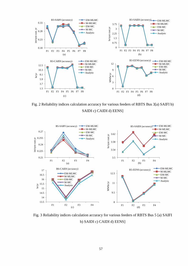
57

Fig. 2 Reliability indices calculation accuracy for various feeders of RBTS Bus 3[a) SAIFI b)

SAIDI c) CAIDI d) EENS]

0.18

0.23

0.28

0.33

F1 F2 F3 F4 F5 F6 F7 F8

int/

syst

cu

st. yr

(a)

B3-SAIFI (accuracy) EM-MLMC

M-MLMC

EM-MC

M-MC

Analytic

0

0.75

1.5

2.25

3

3.75

F1 F2 F3 F4 F5 F6 F7 F8

hr/

syst

cu

st.y

r

(b)

B3-SAIDI (accuracy) EM-MLMC

M-MLMC

EM-MC

M-MC

Analytic

1.5

3.7

5.9

8.1

10.3

12.5

F1 F2 F3 F4 F5 F6 F7 F8

hr/

yr

(c)

B3-CAIDI (accuracy) EM-MLMC M-MLMC EM-MC M-MC Analytic

0

3

6

9

12

F1 F2 F3 F4 F5 F6 F7 F8

MW

hr/

yr

(d)

B3-EENS (accuracy) EM-MLMC M-MLMC EM-MC M-MC Analytic

Fig. 3 Reliability indices calculation accuracy for various feeders of RBTS Bus 5 [a) SAIFI

b) SAIDI c) CAIDI d) EENS]

0.21

0.225

0.24

0.255

0.27

F1 F2 F3 F4

int/

syst

cu

st.y

r

(a)

B5-SAIFI (accuracy) EM-MLMC

M-MLMC

EM-MC

M-MC

Analytic

3.5

3.54

3.58

3.62

F1 F2 F3 F4

hr/

syst

cu

st.y

r

(b)

B5-SAIDI (accuracy) EM-MLMC

M-MLMC

EM-MC

M-MC

Analytic

13.5

14

14.5

15

15.5

16

16.5

17

F1 F2 F3 F4

hr/

yr

(c)

B6-CAIDI (accuracy)

EM-MLMC

M-MLMC

EM-MC

M-MC

Analytic

8

9.5

11

12.5

F1 F2 F3 F4

MW

hr/

yr

(d)

B5-EENS (accuracy) EM-MLMC

M-MLMC

EM-MC

M-MC

Analytic

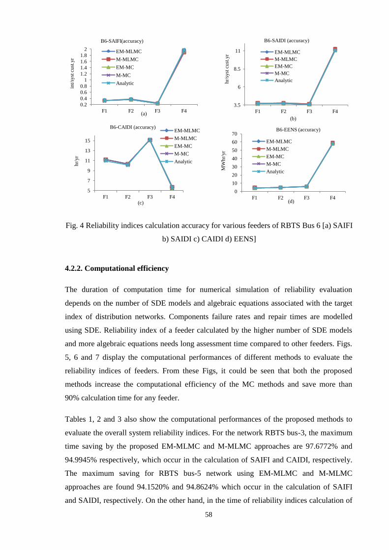
58

4.2.2. Computational efficiency

The duration of computation time for numerical simulation of reliability evaluation

depends on the number of SDE models and algebraic equations associated with the target

index of distribution networks. Components failure rates and repair times are modelled

using SDE. Reliability index of a feeder calculated by the higher number of SDE models

and more algebraic equations needs long assessment time compared to other feeders. Figs.

5, 6 and 7 display the computational performances of different methods to evaluate the

reliability indices of feeders. From these Figs, it could be seen that both the proposed

methods increase the computational efficiency of the MC methods and save more than

90% calculation time for any feeder.

Tables 1, 2 and 3 also show the computational performances of the proposed methods to

evaluate the overall system reliability indices. For the network RBTS bus-3, the maximum

time saving by the proposed EM-MLMC and M-MLMC approaches are 97.6772% and

94.9945% respectively, which occur in the calculation of SAIFI and CAIDI, respectively.

The maximum saving for RBTS bus-5 network using EM-MLMC and M-MLMC

approaches are found 94.1520% and 94.8624% which occur in the calculation of SAIFI

and SAIDI, respectively. On the other hand, in the time of reliability indices calculation of

Fig. 4 Reliability indices calculation accuracy for various feeders of RBTS Bus 6 [a) SAIFI

b) SAIDI c) CAIDI d) EENS]

0.2

0.4

0.6

0.8

1

1.2

1.4

1.6

1.8

2

F1 F2 F3 F4

int/

syst

cu

st.y

r

(a)

B6-SAIFI(accuracy)

EM-MLMC

M-MLMC

EM-MC

M-MC

Analytic

3.5

6

8.5

11

F1 F2 F3 F4

hr/

syst

cu

st.y

r

(b)

B6-SAIDI (accuracy)

EM-MLMC

M-MLMC

EM-MC

M-MC

Analytic

5

7

9

11

13

15

F1 F2 F3 F4

hr/

yr

(c)

B6-CAIDI (accuracy) EM-MLMC

M-MLMC

EM-MC

M-MC

Analytic

0

10

20

30

40

50

60

70

F1 F2 F3 F4

MW

hr/

yr

(d)

B6-EENS (accuracy)

EM-MLMC

M-MLMC

EM-MC

M-MC

Analytic

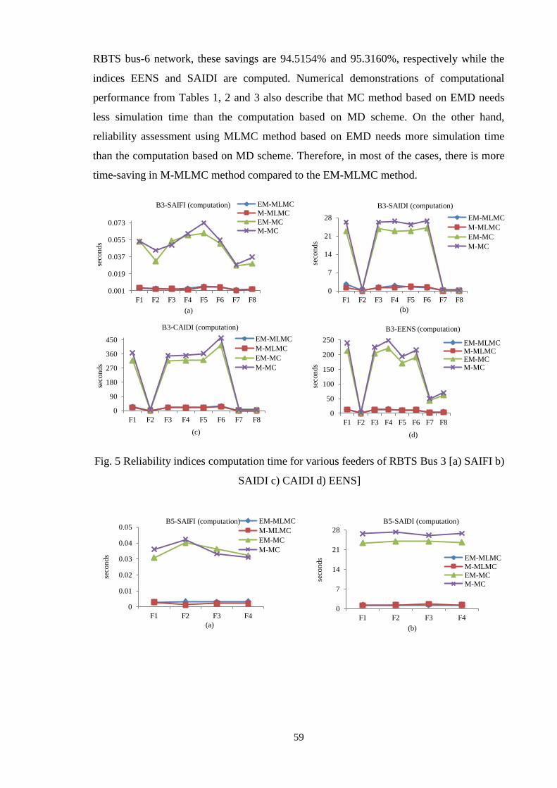
59

RBTS bus-6 network, these savings are 94.5154% and 95.3160%, respectively while the

indices EENS and SAIDI are computed. Numerical demonstrations of computational

performance from Tables 1, 2 and 3 also describe that MC method based on EMD needs

less simulation time than the computation based on MD scheme. On the other hand,

reliability assessment using MLMC method based on EMD needs more simulation time

than the computation based on MD scheme. Therefore, in most of the cases, there is more

time-saving in M-MLMC method compared to the EM-MLMC method.

Fig. 5 Reliability indices computation time for various feeders of RBTS Bus 3 [a) SAIFI b)


0.001

0.019

0.037

0.055

0.073

F1 F2 F3 F4 F5 F6 F7 F8

seco

nd

s

(a)

B3-SAIFI (computation) EM-MLMC

M-MLMC

EM-MC

M-MC

0

7

14

21

28

F1 F2 F3 F4 F5 F6 F7 F8

seco

nd

s (b)

B3-SAIDI (computation)

EM-MLMC

M-MLMC

EM-MC

M-MC

0

90

180

270

360

450

F1 F2 F3 F4 F5 F6 F7 F8

seco

nd

s

(c)

B3-CAIDI (computation)

EM-MLMC

M-MLMC

EM-MC

M-MC

0

50

100

150

200

250

F1 F2 F3 F4 F5 F6 F7 F8

seco

nd

s

(d)

B3-EENS (computation)

EM-MLMC M-MLMC EM-MC M-MC

0

0.01

0.02

0.03

0.04

0.05

F1 F2 F3 F4

seco

nd

s

(a)

B5-SAIFI (computation) EM-MLMC

M-MLMC

EM-MC

M-MC

0

7

14

21

28

F1 F2 F3 F4

seco

nd

s

(b)


EM-MLMC

M-MLMC

EM-MC

M-MC

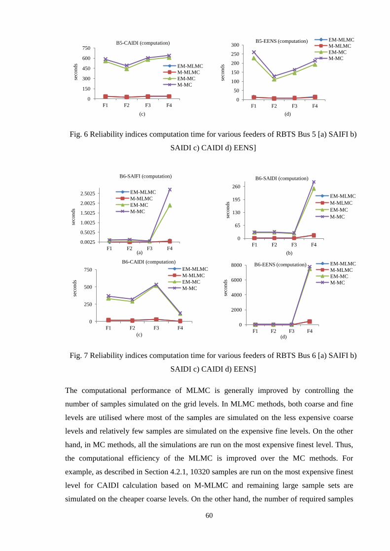
60





The computational performance of MLMC is generally improved by controlling the

number of samples simulated on the grid levels. In MLMC methods, both coarse and fine

levels are utilised where most of the samples are simulated on the less expensive coarse

levels and relatively few samples are simulated on the expensive fine levels. On the other

hand, in MC methods, all the simulations are run on the most expensive finest level. Thus,

the computational efficiency of the MLMC is improved over the MC methods. For

example, as described in Section 4.2.1, 10320 samples are run on the most expensive finest

level for CAIDI calculation based on M-MLMC and remaining large sample sets are

simulated on the cheaper coarse levels. On the other hand, the number of required samples

0

150

300

450

600

750

F1 F2 F3 F4

seco

nd

s

(c)


EM-MLMC

M-MLMC

EM-MC

M-MC

0

50

100

150

200

250

300

F1 F2 F3 F4

seco

nd

s

(d)

B5-EENS (computation) EM-MLMC

M-MLMC

EM-MC

M-MC

0.0025

0.5025

1.0025

1.5025

2.0025

2.5025

F1 F2 F3 F4

seco

nd

s

(a)

B6-SAIFI (computation)

EM-MLMC

M-MLMC

EM-MC

M-MC

0

65

130

195

260

F1 F2 F3 F4

seco

nd

s

(b)


EM-MLMC

M-MLMC

EM-MC

M-MC

0

250

500

750

F1 F2 F3 F4

seco

nd

s

(c)


EM-MLMC

M-MLMC

EM-MC

M-MC

0

2000

4000

6000

8000

F1 F2 F3 F4

seco

nd

s

(d)

B6-EENS (computation) EM-MLMC

M-MLMC

EM-MC

M-MC

61

for M-MC is 32032 and all the simulations are performed on the most expensive finest

level ( ). Therefore, overall computation time is saved by MLMC method.

5. Conclusion

In this paper, we have applied new techniques based on multilevel Monte Carlo method for

estimating the reliability of distribution systems. Two methods, Euler-Maruyama MLMC

and Milstein MLMC have been proposed based on two discretisation schemes of SDE

model solutions of reliability indices. The main objective of the methods is to reduce the

calculation time of sequential Monte Carlo based reliability evaluation. The effectiveness

of the proposed methods is validated on three test systems, RBTS-buses 3, 5 and 6.

From the results, we can conclude that both MLMC approaches based on discretisation

schemes reduce the simulation running time and speed up the reliability evaluation process

compared to MC method. Reasonably accurate reliability indices are found using these

new methods.

In the future paper, we will concentrate on several issues. The current study only deals

with the determination of reliability indices mean values while in the future, the proposed

method for determining the probability distributions [24] of indices will be implemented

and its capability will be compared with the MCS. The effects of varying pre-determined

parameters (such as drift, volatility values) on reliability evaluation will be carried out.

Finally, we will compare the performance of MLMC method with other advanced MC

methods [25].

References

[1] Allan, R.: 'Reliability evaluation of power systems' (Springer Science & Business

Media, 2013)

[2] Alkuhayli, A. A., Raghavan, S., Chowdhury, B. H.: 'Reliability evaluation of

distribution systems containing renewable distributed generations', Proc. North

American Power Symposium (NAPS), 2012, pp. 1-6

[3] Goel, L., Billinton, R.: 'Evaluation of interrupted energy assessment rates in

distribution systems', IEEE Trans. Power Delivery, 1991, 6, pp. 1876-1882

[4] Billinton, R., Acharya, J.: 'Weather-based distribution system reliability evaluation',

IEE Proc.- Gener. Transm. Distrib., 2006, 153, pp. 499-506

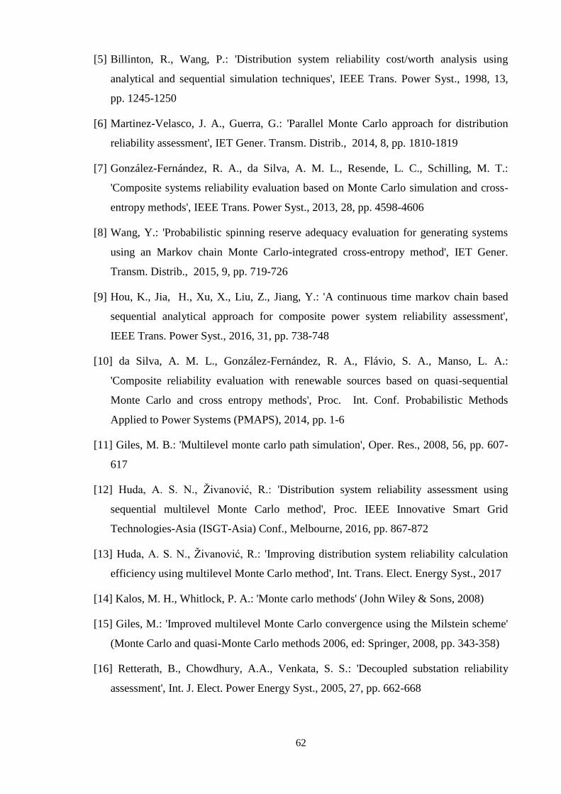
62

[5] Billinton, R., Wang, P.: 'Distribution system reliability cost/worth analysis using

analytical and sequential simulation techniques', IEEE Trans. Power Syst., 1998, 13,

pp. 1245-1250

[6] Martinez-Velasco, J. A., Guerra, G.: 'Parallel Monte Carlo approach for distribution

reliability assessment', IET Gener. Transm. Distrib., 2014, 8, pp. 1810-1819

[7] González-Fernández, R. A., da Silva, A. M. L., Resende, L. C., Schilling, M. T.:

'Composite systems reliability evaluation based on Monte Carlo simulation and cross-

entropy methods', IEEE Trans. Power Syst., 2013, 28, pp. 4598-4606

[8] Wang, Y.: 'Probabilistic spinning reserve adequacy evaluation for generating systems

using an Markov chain Monte Carlo-integrated cross-entropy method', IET Gener.

Transm. Distrib., 2015, 9, pp. 719-726

[9] Hou, K., Jia, H., Xu, X., Liu, Z., Jiang, Y.: 'A continuous time markov chain based

sequential analytical approach for composite power system reliability assessment',

IEEE Trans. Power Syst., 2016, 31, pp. 738-748

[10] da Silva, A. M. L., González-Fernández, R. A., Flávio, S. A., Manso, L. A.:

'Composite reliability evaluation with renewable sources based on quasi-sequential

Monte Carlo and cross entropy methods', Proc. Int. Conf. Probabilistic Methods

Applied to Power Systems (PMAPS), 2014, pp. 1-6

[11] Giles, M. B.: 'Multilevel monte carlo path simulation', Oper. Res., 2008, 56, pp. 607-

617

[12] Huda, A. S. N., Živanović, R.: 'Distribution system reliability assessment using

sequential multilevel Monte Carlo method', Proc. IEEE Innovative Smart Grid

Technologies-Asia (ISGT-Asia) Conf., Melbourne, 2016, pp. 867-872

[13] Huda, A. S. N., Živanović, R.: 'Improving distribution system reliability calculation

efficiency using multilevel Monte Carlo method', Int. Trans. Elect. Energy Syst., 2017

[14] Kalos, M. H., Whitlock, P. A.: 'Monte carlo methods' (John Wiley & Sons, 2008)

[15] Giles, M.: 'Improved multilevel Monte Carlo convergence using the Milstein scheme'

(Monte Carlo and quasi-Monte Carlo methods 2006, ed: Springer, 2008, pp. 343-358)

[16] Retterath, B., Chowdhury, A.A., Venkata, S. S.: 'Decoupled substation reliability

assessment', Int. J. Elect. Power Energy Syst., 2005, 27, pp. 662-668

63

[17] Harrison, J. M.: 'Brownian motion and stochastic flow systems' (Wiley New York,

1985)

[18] Oksendal, B.: 'Stochastic differential equations: an introduction with applications'

(Springer Science & Business Media, 2013)

[19] Giles, M. B.: 'Multilevel Monte Carlo for basket options', Proc. Winter Simulation

Conf., 2009, pp. 1283-1290

[20] Kloeden, P. E., Platen, E.: 'Higher-order implicit strong numerical schemes for

stochastic differential equations', J. Stat. Phys., 1992, 66, pp. 283-314

[21] Platen, E.: 'An introduction to numerical methods for stochastic differential equations',

Acta Numerica, 1999, 8, pp. 197-246

[22] Billinton, R., Jonnavithula, S.: 'A test system for teaching overall power system

reliability assessment', IEEE Trans. Power Syst., 1996, 11, pp. 1670-1676

[23] Allan, R. N., Billinton, R. Sjarief, I.: 'A reliability test system for educational

purposes-basic distribution system data and results', IEEE Trans. Power syst., 1991, 6,

pp. 813-820

[24] Bierig, C., Chernov, A.: 'Approximation of probability density functions by the

Multilevel Monte Carlo Maximum Entropy method', J. Comput. Phys., 2016, 314, pp.

661-681

[25] González-Fernández, R. A., da Silva, A. M. L.: 'Reliability assessment of time-

dependent systems via sequential cross-entropy Monte Carlo simulation', IEEE Trans.

Power Syst., 2011, 26, pp. 2381-2389

64

Chapter 4

Component Importance Analysis

65


Title of Paper Study effect of components availability on distribution system reliability through Multilevel

Monte Carlo method





manuscript style

Publication Details A. S. Nazmul Huda and Rastko Živanović (2018) Study effect of components availability on

distribution system reliability through Multilevel Monte Carlo method, IEEE Transactions on

Industrial informatics. Published (Early access)

Link: https://ieeexplore.ieee.org/document/8506413

Principal author


(Candidate)

A. S. Nazmul Huda



manuscript.





paper.









Signature

Date 13.08.2018

https://ieeexplore.ieee.org/document/8506413

66

Study effect of components availability on distribution system reliability through

Multilevel Monte Carlo method

Abstract— Reliability model of a power distribution system is influenced by its

components reliability and availability. The paper investigates the effect of some basic

protection components availability on the distribution system reliability improvement. For

this purpose, we use a new approach called Multilevel Monte Carlo to speed up the

conventional Monte Carlo simulation based reliability assessment. The proposed method is

implemented through solving stochastic differential equations of the system components

random failure process using Milstein discretisation scheme. To illustrate the proposed

method, two commonly used reliability indices are evaluated for a test distribution

network.

Index Terms— components importance, reliability, Multilevel Monte Carlo, distribution

system, Milstein discretisation.

I. Introduction

Reliability is one of the key design considerations for an electric distribution system

(EDS). A highly reliable EDS ensures a smaller number of supply interruptions and their

short duration. Due to the simple design and comparatively low cost, radial distribution

systems are usually popular [1]. In reliability evaluation, components availability effect or

importance study investigates the comparative importance of individual components or

groups of components to system performance improvement [2, 3]. An EDS consists of

different components such as circuit breakers, fuses, main feeder sections, lateral sections,

disconnecting switches and low voltage transformers, etc. The expansion of EDS by the

inclusion of alternative supply source is also used to improve the network reliability level.

Any component failure could lead to interruption of a load point (LP) in a radial system.

Three basic primary reliability indices (RI) of an EDS are mean values of Failure Time

(FT), Repair Time (RT) and Annual Unavailability (AU) [4, 5]. The failure period and the

number of customers affected due to a component failure can be reduced by making the

availability of the protection components and alternative supply [6, 7]. Therefore, the level

of reliability of an EDS primarily relies on the reliability of the basic components and the

arrangement of these components in the EDS. In this paper, some case studies based on a

benchmark radial distribution system is analyzed by considering different components

configurations to show their importance in reliability improvement.

67

For reliability studies, generally computational tools utilize analytical methods or crude

Monte Carlo (MC) method [5, 8]. MC method is usually preferred over the analytical

techniques because the impact of uncertainties of RI variables can be incorporated. The

importance of considering the uncertainties in EDS planning is widely recognised by the

utility industries. The convergence of MC simulation is reached when the estimated

variance lies within a specified tolerance level. Therefore, the efficiency of MC based

method decreases when the system is very reliable and the estimation of the rare-event

probability consumes a large time [9]. Hence one of the main issues in simple MC method

or Markov Chain MC [10] is their slow convergence speed for achieving high simulation

accuracy. The incorporation of stochastic uncertainties and reliability improvement by

adding new components can significantly increase the system complexity and therefore, RI

evaluation time by MC methods is prolonged.

In order to enhance the convergence speed of the MC method in power system reliability

assessment applications, various variance reduction techniques (VRT) have been proposed,

such as control variates, antithetic variates [11] and state space pruning [12] etc. Through

VRT, the expected value of an output random variable can be obtained with reduced

simulation time by maintaining an accuracy level. VRT based on importance sampling

which are known as cross-entropy (CE) methods have been utilized extensively in power

system reliability applications in order to speed up computation. The research studies are

generally carried out for the reliability evaluation of the composite generation and

transmission systems [13-16]. For example, CE method was successfully applied in

generating capacity reliability problems [14] [17-19] and short-term reliability [15]. In the

CE-based method, the state variables are properly distorted in accordance with an

optimization process. Due to the optimal distortion, the rate of failure events is more

frequent and the convergence rate of the algorithm is significantly enhanced. Later, this

method was used for developing more advanced MC-based methods, such as quasi-

sequential/CE [18], pseudo-chronological/CE [20], and sequential/CE [14]. In all methods

using CE, significant simulation speed was accelerated compared to non-CE version [21].

However, these methods were unable to obtain probability distributions of indices. In one

study, an improved importance sampling was applied to generation, transmission line and

load states which reduced the computational effort [22]. Additionally, another VRT based

on subset simulation has been successfully applied in reliability estimation [23] where a

small failure probability is represented as the product of larger conditional probabilities.

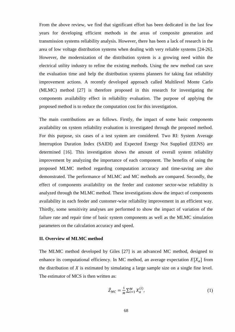
68

From the above review, we find that significant effort has been dedicated in the last few

years for developing efficient methods in the areas of composite generation and

transmission systems reliability analysis. However, there has been a lack of research in the

area of low voltage distribution systems when dealing with very reliable systems [24-26].

However, the modernization of the distribution system is a growing need within the

electrical utility industry to refine the existing methods. Using the new method can save

the evaluation time and help the distribution systems planners for taking fast reliability

improvement actions. A recently developed approach called Multilevel Monte Carlo

(MLMC) method [27] is therefore proposed in this research for investigating the

components availability effect in reliability evaluation. The purpose of applying the

proposed method is to reduce the computation cost for this investigation.

The main contributions are as follows. Firstly, the impact of some basic components

availability on system reliability evaluation is investigated through the proposed method.

For this purpose, six cases of a test system are considered. Two RI: System Average

Interruption Duration Index (SAIDI) and Expected Energy Not Supplied (EENS) are

determined [16]. This investigation shows the amount of overall system reliability

improvement by analyzing the importance of each component. The benefits of using the

proposed MLMC method regarding computation accuracy and time-saving are also

demonstrated. The performance of MLMC and MC methods are compared. Secondly, the

effect of components availability on the feeder and customer sector-wise reliability is

analyzed through the MLMC method. These investigations show the impact of components

availability in each feeder and customer-wise reliability improvement in an efficient way.

Thirdly, some sensitivity analyses are performed to show the impact of variation of the

failure rate and repair time of basic system components as well as the MLMC simulation

parameters on the calculation accuracy and speed.

II. Overview of MLMC method

The MLMC method developed by Giles [27] is an advanced MC method, designed to

enhance its computational efficiency. In MC method, an average expectation from

the distribution of is estimated by simulating a large sample size on a single fine level.

The estimator of MCS is then written as:

(1)

69

where is the target reliability index and

is the ith

sample of , is the MC sample

size and is the estimated variance. The root-mean-square-error (RMSE) value

of the MC estimator is therefore, . A sample size is required to

achieve an accuracy level of . This means a large sample size is required to be simulated

on the finest level for a highly accurate model.

In the MC method, the calculation of an expectation is carried out on a single fine level

. is a nonnegative integer. In this level, both the accuracy and computation cost of

the expectation are high.

In the MLMC method, same expectation is approximated using multiple parts or levels

instead of single-level . The multiple levels can be divided as . Here

and are the coarsest and finest discretisation levels, respectively. On each level,

expectations are estimated using different number of samples in a way which minimises

the overall variance for a defined accuracy. Initially, a large number of samples are

simulated on . The purpose of the next level is to add a correction value that

decreases the bias. Based on this correction value, the expected difference from one level

to the next fine level is added, until level is reached. By this way, the less correct

estimation on the coarsest grid is successively corrected by the approximations on the

subsequent fine grids and thus the finest grid accuracy is achieved. The MLMC

expectation can be expressed as:

(2)

Now the estimator for the above MLMC expectation is

(3)

where is an unbiased estimator for using sample and is the MCS estimator

for using samples from .

and (4)

(5)

70

is approximated using the difference of expectation between coarse and fine

level as

. and

are estimated using two different time-step

sizes and , respectively [28]. where

(6)

. (7)

On , a large and fixed value timestep is used to generate a large sample size . This

means that the coarsest level is the computationally cheapest level and the simulation time

increases with the increase of level. The statistical properties of are unchanged whether

the estimation of from level to or from to .

This means that both and have the same expected value, i.e.,

. The convergence criterion in the MLMC method depends on the desired

RMSE value which can be expressed as follows:

(8)

In order to obtain the value of , it is enough to ensure that both the estimated

variance and approximation error are less than . The different number of samples

ensures that the variance of the MLMC estimator is less than . As the level increases

from the coarsest level and moves to finer level, number of samples on each level is

decreased by setting an optimal . The optimal is chosen as [27]:

(9)

where the cost to compute one sample on the level is for a constant and

some . is the rate of computation cost increase with level .

In the case of weak convergence, the test tries to confirm that .

Consider, the convergence rate of with for constant is measured by a

positive value , i.e., [27]. The remaining error is

and the target convergence criterion is

. is assumed as the convergence rate of variance with for a constant i.e.,

For a constant , the computational complexity of the MLMC estimator is

bounded as follows [27]:

71

(10)

III. Proposed methodology

The description of the proposed methodology can be presented as follows:

1. Read all the feeder length, failure and repair time data of components. Some simulation

parameters are also defined: sample size for MLMC convergence (N), initial sample size

( ), accuracy level ( ), drift ( ) and volatility ( ). is the rate of change of average

value of stochastic process and is the degree of variation of stochastic process over time.

2. Generate artificial uptime and downtime histories of components. The variables and

of each component are considered to be distributed using exponential probability

function as (11) and (12), respectively.

(11)

(12)

where and are the uptime and downtime histories of a component I ,

respectively. is the mean failure rate (FR) (failure/year) and is mean RT (hour/failure)

of . , are uniformly distributed random variables between [0, 1].

3. Construct the stochastic differential equations (SDEs) of and on . We

propose to model SDE by the Brownian motion due to its simplest form [29]. If is the

of at a time , then SDE model of with defined , and an initial FT

can be written using the Brownian motion, on the whole time interval [ ] [30]

as:

(13)

4. Solve the SDE by Milstein discretisation which is proposed for this study [28]. The

discretisation scheme with timesteps, step size and Brownian increments

can be written as:

(14)

72

where . are

independent and normally distributed random variables.

5. Express the in (11) using the SDE model (14) of as:

(15)

Similarly, can be determined using SDE model of . For modeling, µ and σ

values are assumed equal as model. For simplification, we model the as a function

of . If is a constant for and , then initial of is . can be

therefore expressed as:

(16)

6. Calculate average AU ( ) of as follows

(17)

where is the desired number of simulated periods.

7. Repeat steps (2)-(6) for each component failure in the EDS.

8. Find the affected LPs by each component failure by the direct method [31] and

determine LP AU ( ) as:

(18)

where is the total number of component failures that interrupt the service of .

9. Repeat steps (2)-(8) for each LP in the EDS and evaluate the proposed system RI as (19)

and (20):

(19)

(20)

where and are the number of customers and average load at , respectively.

and are the total numbers of customers served and LPs in the EDS, respectively.

73

10. Calculate the sum of the system RI values on levels . Repeat the whole process

until the number of samples is reached to N.

11. To test the convergence criterion, set a minimum finest level of the MLMC method on

. Generate the numbers of samples on levels using . Also, update

the sum of the RI values on each level.

12. Determine the absolute average value of reliability index and variance

on each level l.

13. Determine the optimal number of samples on each level based on

(9). Compare the optimal with the calculated on that level. If , determine

extra samples on each level as required.

14. Update the and on each level. The optimal on each level keeps

.

15. Test the weak convergence as mentioned in Section 2, which confirms the remaining

bias error is smaller than .

16. Set , if the bias error is greater than . Repeat the simulation from the

step (11) until the target level of accuracy is reached. Finally, compute the overall

multilevel estimator for each system reliability index using (3).

IV. Test system

A network connected to Bus 4 (B4) of the Roy Billinton Test system (RBTS) [32] is

proposed to conduct the research. The single line diagram of the test system is provided in

Appendix A. RBTS B4 is a typical urban EDS with seven (F1-F7) main feeders. A primary

feeder begins with a circuit breaker at the distribution substation and carries electricity to

the customer load points through lateral section. A lateral section consists of fuse, line and

low voltage transformer. The feeders (types and lengths), customers and load data of the

EDS are taken from [33]. For investigating components importance by MLMC method, six

case studies are carried out by varying the availability of the components as shown in

Table I. Case A is assumed as a base Case or ideal Case. For both MC and MLMC

methods, a target of 0.001 was specified. All simulations are performed with an Intel

Core i7‐4790 3.60 GHz processor.

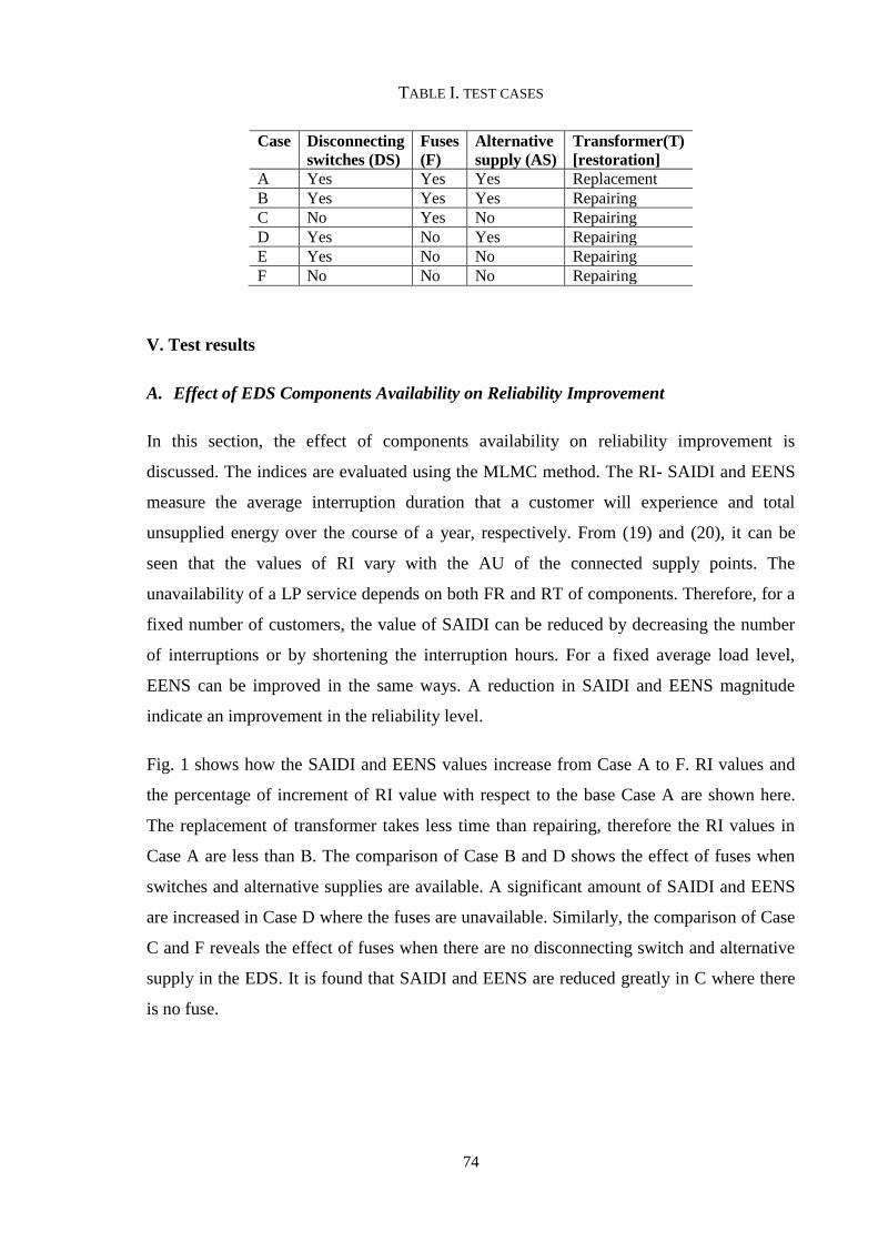
74

TABLE I. TEST CASES

Case Disconnecting

switches (DS)

Fuses

(F)

Alternative

supply (AS)

Transformer(T)

[restoration]

A Yes Yes Yes Replacement

B Yes Yes Yes Repairing

C No Yes No Repairing

D Yes No Yes Repairing

E Yes No No Repairing

F No No No Repairing

V. Test results

A. Effect of EDS Components Availability on Reliability Improvement

In this section, the effect of components availability on reliability improvement is

discussed. The indices are evaluated using the MLMC method. The RI- SAIDI and EENS

measure the average interruption duration that a customer will experience and total

unsupplied energy over the course of a year, respectively. From (19) and (20), it can be

seen that the values of RI vary with the AU of the connected supply points. The

unavailability of a LP service depends on both FR and RT of components. Therefore, for a

fixed number of customers, the value of SAIDI can be reduced by decreasing the number

of interruptions or by shortening the interruption hours. For a fixed average load level,

EENS can be improved in the same ways. A reduction in SAIDI and EENS magnitude

indicate an improvement in the reliability level.

Fig. 1 shows how the SAIDI and EENS values increase from Case A to F. RI values and

the percentage of increment of RI value with respect to the base Case A are shown here.

The replacement of transformer takes less time than repairing, therefore the RI values in

Case A are less than B. The comparison of Case B and D shows the effect of fuses when

switches and alternative supplies are available. A significant amount of SAIDI and EENS

are increased in Case D where the fuses are unavailable. Similarly, the comparison of Case

C and F reveals the effect of fuses when there are no disconnecting switch and alternative

supply in the EDS. It is found that SAIDI and EENS are reduced greatly in C where there

is no fuse.

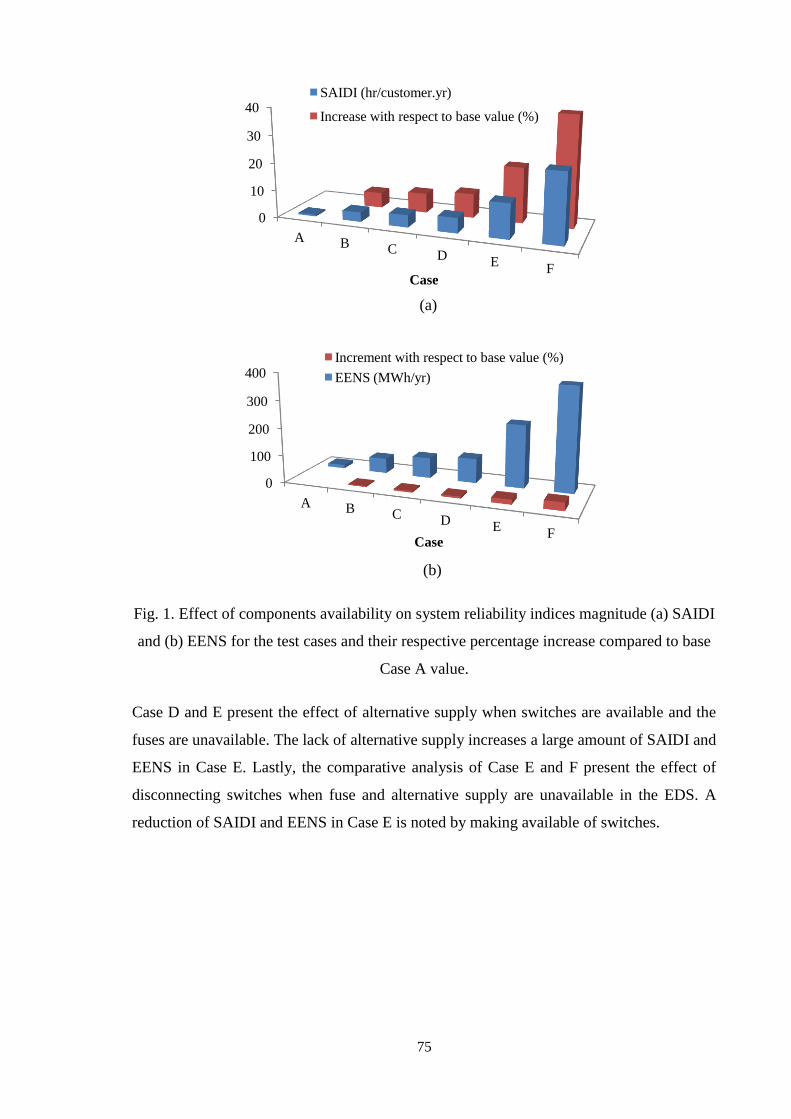
75

(a)

(b)

Fig. 1. Effect of components availability on system reliability indices magnitude (a) SAIDI

and (b) EENS for the test cases and their respective percentage increase compared to base

Case A value.

Case D and E present the effect of alternative supply when switches are available and the

fuses are unavailable. The lack of alternative supply increases a large amount of SAIDI and

EENS in Case E. Lastly, the comparative analysis of Case E and F present the effect of

disconnecting switches when fuse and alternative supply are unavailable in the EDS. A

reduction of SAIDI and EENS in Case E is noted by making available of switches.

0

10

20

30

40

A B C D E

F Case

SAIDI (hr/customer.yr)

Increase with respect to base value (%)

0

100

200

300

400

A B C D E F

Case

Increment with respect to base value (%)

EENS (MWh/yr)

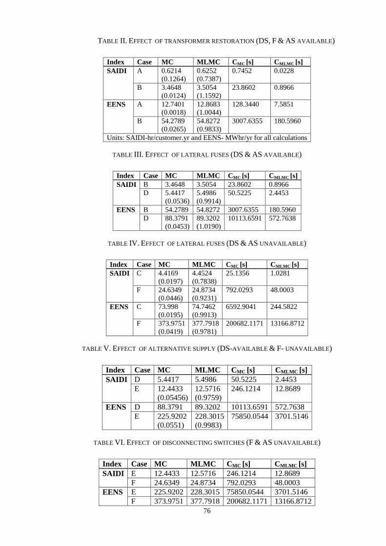
76

TABLE II. EFFECT OF TRANSFORMER RESTORATION (DS, F & AS AVAILABLE)

Index Case MC MLMC CMC [s] CMLMC [s]

SAIDI

A 0.6214

(0.1264)

0.6252

(0.7387)

0.7452 0.0228

B 3.4648

(0.0124)

3.5054

(1.1592)

23.8602 0.8966

EENS

A 12.7401

(0.0018)

12.8683

(1.0044)

128.3440 7.5851

B 54.2789

(0.0265)

54.8272

(0.9833)

3007.6355 180.5960

Units: SAIDI-hr/customer.yr and EENS- MWhr/yr for all calculations

TABLE III. EFFECT OF LATERAL FUSES (DS & AS AVAILABLE)


SAIDI

B 3.4648 3.5054 23.8602 0.8966

D 5.4417

(0.0536)

5.4986

(0.9914)

50.5225 2.4453

EENS

B 54.2789 54.8272 3007.6355 180.5960

D 88.3791

(0.0453)

89.3202

(1.0190)

10113.6591 572.7638

TABLE IV. EFFECT OF LATERAL FUSES (DS & AS UNAVAILABLE)


SAIDI

C 4.4169

(0.0197)

4.4524

(0.7838)

25.1356 1.0281

F 24.6349

(0.0446)

24.8734

(0.9231)

792.0293 48.0003

EENS

C 73.998

(0.0195)

74.7462

(0.9913)

6592.9041 244.5822

F 373.9751

(0.0419)

377.7918

(0.9781)

200682.1171 13166.8712

TABLE V. EFFECT OF ALTERNATIVE SUPPLY (DS-AVAILABLE & F- UNAVAILABLE)


SAIDI

D 5.4417 5.4986 50.5225 2.4453

E 12.4433

(0.05456)

12.5716

(0.9759)

246.1214 12.8689

EENS

D 88.3791 89.3202 10113.6591 572.7638

E 225.9202

(0.0551)

228.3015

(0.9983)

75850.0544 3701.5146

TABLE VI. EFFECT OF DISCONNECTING SWITCHES (F & AS UNAVAILABLE)


SAIDI

E 12.4433 12.5716 246.1214 12.8689

F 24.6349 24.8734 792.0293 48.0003

EENS

E 225.9202 228.3015 75850.0544 3701.5146

F 373.9751 377.7918 200682.1171 13166.8712

77

B. Analysis of Components Availability Effect on System Reliability Evaluation through

MLMC Method

The results showing the reliability evaluation accuracy and time for all the cases using both

methods are shown in Tables II-VI. The values inside the first bracket are the percentage of

absolute values of the evaluation errors by MC (EMC) and MLMC (EMLMC) which are

computed by comparing with the analytical values. CMC and CMLMC are the required CPU

time in second (s), by the MC and MLMC methods, respectively. Speedup rate of the

MLMC based reliability evaluation is calculated as follows:

(23)

1) Case A

In Case A, we consider the availability of switches, fuses, alternative supply and

replacement of transformers. The maximum EMLMC value is 1.0044% [EENS]. As

expected, the MC method needs the maximum CPU time of 2.1390 min for EENS

calculation while MLMC needs only 7.5851 s. So, there is speedup around 90.6679%

when compared with the MC.

2) Case B

The difference between Case A and B is transformer action restoration process. In Case B,

transformer action is restored by repairing rather than replacing. The maximum EMLMC in

MLMC is 1.1592% [SAIDI]. The MC and MLMC methods spent the maximum CPU time

of 50.1272 min and 3.0099 min [EENS] for this Case, respectively. Therefore, the

computation speedup using MLMC is around 93.9954%.

3) Case C

In Case C, the unavailability of disconnecting switches and alternative supply is

considered. The maximum EMLMC value is 0.9913% [EENS]. For this Case, the MC and

MLMC algorithms spent the maximum CPU time of 1.8313 hr and 4.0763 min,

respectively. Therefore, the speedup of the proposed method in relation to the MC is

around 96.2902%. As it could be expected, the system reliability is deteriorated in Case C

and the CPU time increases.

78

4) Case D

The difference between Case B and D is the unavailability of fuses in Case D. The

maximum EMLMC value is 1.0190% [EENS]. The MC algorithm spent the maximum CPU

time of 2.8093 hr. The MLMC method spent 9.5460 min and speedup is around 94.3367%.

5) Case E

In Case E, the unavailability of alternative supply is considered. The maximum EMLMC

value is 0.9983% [EENS]. The MC algorithm spent the maximum CPU time of 21.0694 hr

[EENS]. The MLMC method spent 1.0281 hr and speedup is around 95.1199%.

6) Case F

The difference between Case B and F is the unavailability of disconnecting switches, fuses

and alternative supply in Case F. The maximum EMLMC value is 0.9781% [EENS]. The MC

method spent the maximum CPU time of 55.7450 hr for this Case. The MLMC method

spent 3.6574 hr and speedup in relation to the MC is around 93.4389%.

C. Analysis of Components Availability Effect on Feeder Reliability Evaluation through

MLMC Method

By using MLMC method, the RI value for each feeder of the test system for all the cases

and their CPU time is shown in Fig. 2. The specified feeder SAIDI and EENS increase

gradually from Case A to F. The RI of a feeder depends on the reliability performance of

the connected LPs. The low values of SAIDI and EENS of the feeders are due to the

reduction of connected components outage times and the exclusion of LP transformers. For

F2, F5 and F6, RI values are equal because of having the same connected components. Due

to the effect of random variables, very small fractional difference among these is noticed.

The analysis of components availability effect on feeder based reliability evaluation also

takes less time through using MLMC method and the estimated RI values of feeders are

very close to the true (analytical) values for all the cases.

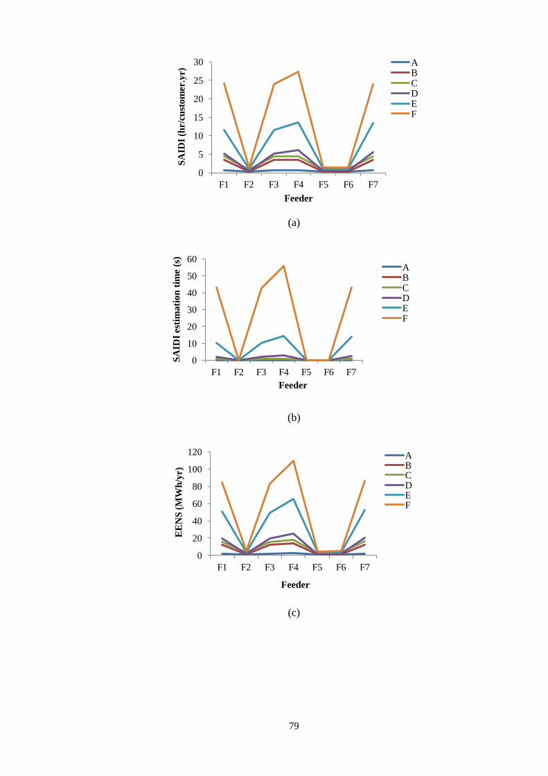
79

(a)

(b)

(c)

0

5

10

15

20

25

30

F1 F2 F3 F4 F5 F6 F7 S

AID

I (h

r/cu

sto

mer

.yr)

Feeder

A B C D E F

0

10

20

30

40

50

60

F1 F2 F3 F4 F5 F6 F7

SA

IDI

esti

mati

on

tim

e (s

)

Feeder

A B C D E F

0

20

40

60

80

100

120

F1 F2 F3 F4 F5 F6 F7

EE

NS

(M

Wh

/yr)

Feeder

A B C D E F

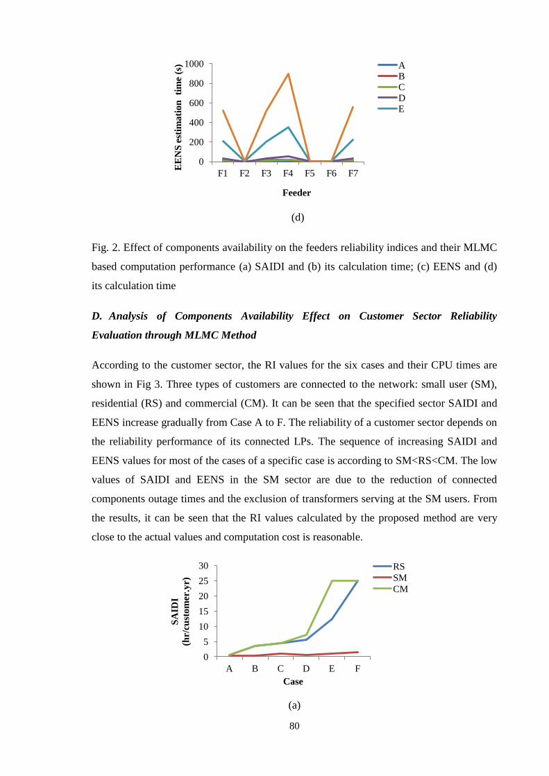
80

(d)

Fig. 2. Effect of components availability on the feeders reliability indices and their MLMC

based computation performance (a) SAIDI and (b) its calculation time; (c) EENS and (d)

its calculation time

D. Analysis of Components Availability Effect on Customer Sector Reliability

Evaluation through MLMC Method

According to the customer sector, the RI values for the six cases and their CPU times are

shown in Fig 3. Three types of customers are connected to the network: small user (SM),

residential (RS) and commercial (CM). It can be seen that the specified sector SAIDI and

EENS increase gradually from Case A to F. The reliability of a customer sector depends on

the reliability performance of its connected LPs. The sequence of increasing SAIDI and

EENS values for most of the cases of a specific case is according to SM<RS<CM. The low

values of SAIDI and EENS in the SM sector are due to the reduction of connected

components outage times and the exclusion of transformers serving at the SM users. From

the results, it can be seen that the RI values calculated by the proposed method are very

close to the actual values and computation cost is reasonable.

(a)

0

200

400

600

800

1000

F1 F2 F3 F4 F5 F6 F7 E

EN

S e

stim

ati

on

ti

me

(s)

Feeder

A B C D E

0

5

10

15

20

25

30

A B C D E F

SA

IDI

(hr/

cust

om

er.y

r)

Case

RS

SM

CM

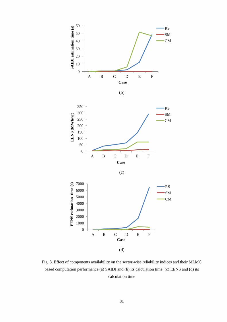
81

(b)

(c)

(d)

Fig. 3. Effect of components availability on the sector-wise reliability indices and their MLMC

based computation performance (a) SAIDI and (b) its calculation time; (c) EENS and (d) its

calculation time

0

10

20

30

40

50

60

A B C D E F S

AID

I es

tim

ati

on

tim

e (s

)

Case

RS

SM

CM

0

50

100

150

200

250

300

350

A B C D E F

EE

NS

(M

Wh

/yr)

Case

RS

SM

CM

0

1000

2000

3000

4000

5000

6000

7000

A B C D E F

EE

NS

est

imati

on

ti

me

(s)

Case

RS

SM

CM

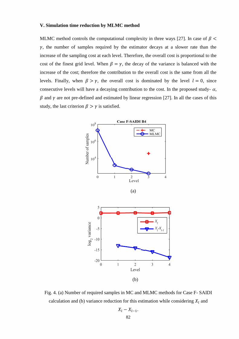
82

V. Simulation time reduction by MLMC method

MLMC method controls the computational complexity in three ways [27]. In case of

, the number of samples required by the estimator decays at a slower rate than the

increase of the sampling cost at each level. Therefore, the overall cost is proportional to the

cost of the finest grid level. When , the decay of the variance is balanced with the

increase of the cost; therefore the contribution to the overall cost is the same from all the

levels. Finally, when , the overall cost is dominated by the level , since

consecutive levels will have a decaying contribution to the cost. In the proposed study- ,

and are not pre-defined and estimated by linear regression [27]. In all the cases of this

study, the last criterion is satisfied.

(a)

(b)

Fig. 4. (a) Number of required samples in MC and MLMC methods for Case F- SAIDI

calculation and (b) variance reduction for this estimation while considering and

.

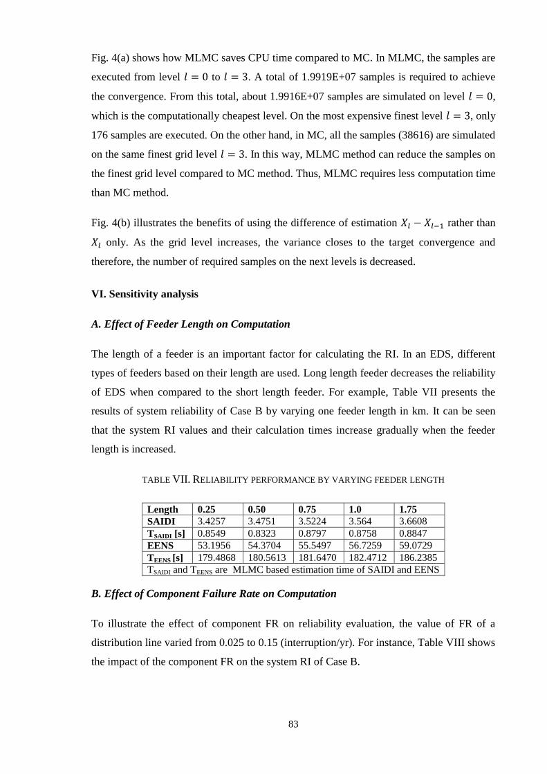
83

Fig. 4(a) shows how MLMC saves CPU time compared to MC. In MLMC, the samples are

executed from level to . A total of 1.9919E+07 samples is required to achieve

the convergence. From this total, about 1.9916E+07 samples are simulated on level ,

which is the computationally cheapest level. On the most expensive finest level , only

176 samples are executed. On the other hand, in MC, all the samples (38616) are simulated

on the same finest grid level . In this way, MLMC method can reduce the samples on

the finest grid level compared to MC method. Thus, MLMC requires less computation time

than MC method.

Fig. 4(b) illustrates the benefits of using the difference of estimation rather than

only. As the grid level increases, the variance closes to the target convergence and

therefore, the number of required samples on the next levels is decreased.

VI. Sensitivity analysis

A. Effect of Feeder Length on Computation

The length of a feeder is an important factor for calculating the RI. In an EDS, different

types of feeders based on their length are used. Long length feeder decreases the reliability

of EDS when compared to the short length feeder. For example, Table VII presents the

results of system reliability of Case B by varying one feeder length in km. It can be seen

that the system RI values and their calculation times increase gradually when the feeder

length is increased.

TABLE VII. RELIABILITY PERFORMANCE BY VARYING FEEDER LENGTH

Length 0.25 0.50 0.75 1.0 1.75

SAIDI 3.4257 3.4751 3.5224 3.564 3.6608

TSAIDI [s] 0.8549 0.8323 0.8797 0.8758 0.8847

EENS 53.1956 54.3704 55.5497 56.7259 59.0729

TEENS [s] 179.4868 180.5613 181.6470 182.4712 186.2385

TSAIDI and TEENS are MLMC based estimation time of SAIDI and EENS

B. Effect of Component Failure Rate on Computation

To illustrate the effect of component FR on reliability evaluation, the value of FR of a

distribution line varied from 0.025 to 0.15 (interruption/yr). For instance, Table VIII shows

the impact of the component FR on the system RI of Case B.

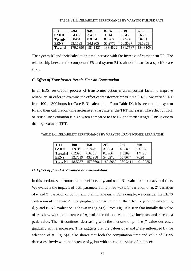
84

TABLE VIII. RELIABILITY PERFORMANCE BY VARYING FAILURE RATE

FR 0.025 0.05 0.075 0.10 0.15

SAIDI 3.4357 3.4655 3.5147 3.543 3.6355

TSAIDI[s] 0.8484 0.8824 0.8763 0.8574 0.8731

EENS 53.1033 54.1905 55.2776 56.3637 58.5355

TEENS[s] 179.7390 181.1427 183.4522 181.7587 184.3109

The system RI and their calculation time increase with the increase of component FR. The

relationship between the component FR and system RI is almost linear for a specific case

study.

C. Effect of Transformer Repair Time on Computation

In an EDS, restoration process of transformer action is an important factor to improve

reliability. In order to examine the effect of transformer repair time (TRT), we varied TRT

from 100 to 300 hours for Case B RI calculation. From Table IX, it is seen that the system

RI and their calculation time increase at a fast rate as the TRT increases. The effect of TRT

on reliability evaluation is high when compared to the FR and feeder length. This is due to

the large value to TRT.

TABLE IX. RELIABILITY PERFORMANCE BY VARYING TRANSFORMER REPAIR TIME

TRT 100 150 200 250 300

SAIDI 1.9719 2.7446 3.5054 4.2589 5.0184

TSAIDI [s] 0.2328 0.6785 0.8966 1.3209 1.9428

EENS 32.7519 43.7988 54.8272 65.8674 76.91

TEENS [s] 48.5787 157.8696 180.5960 280.3414 401.2985

D. Effect of and Variation on Computation

In this section, we demonstrate the effects of and on RI evaluation accuracy and time.

We evaluate the impacts of both parameters into three ways: 1) variation of , 2) variation

of and 3) variation of both and simultaneously. For example, we consider the EENS

evaluation of the Case A. The graphical representation of the effect of on parameters ,

, and EENS evaluation is shown in Fig. 5(a). From Fig., it is seen that initially the value

of is low with the decrease of , and after this the value of increases and reaches a

peak value. Then it continues decreasing with the increase of . The value decreases

gradually with increases. This suggests that the values of and are influenced by the

selection of . Fig. 5(a) also shows that both the computation time and value of EENS

decreases slowly with the increase of , but with acceptable value of the index.

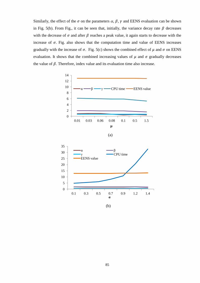
85

Similarly, the effect of the on the parameters , , and EENS evaluation can be shown

in Fig. 5(b). From Fig., it can be seen that, initially, the variance decay rate decreases

with the decrease of and after reaches a peak value, it again starts to decrease with the

increase of . Fig. also shows that the computation time and value of EENS increases

gradually with the increase of . Fig. 5(c) shows the combined effect of and on EENS

evaluation. It shows that the combined increasing values of and gradually decreases

the value of . Therefore, index value and its evaluation time also increase.

(a)

(b)

0

2

4

6

8

10

12

14

0.01 0.03 0.06 0.08 0.1 0.5 1.5

µ

α β γ CPU time EENS value

0

5

10

15

20

25

30

35

0.1 0.3 0.5 0.7 0.9 1.2 1.4 σ

α β γ CPU time EENS value

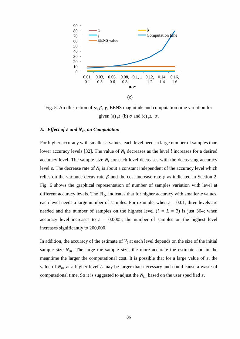
86

(c)

Fig. 5. An illustration of , , , EENS magnitude and computation time variation for

given (a) (b) and (c) , .

E. Effect of and on Computation

For higher accuracy with smaller values, each level needs a large number of samples than

lower accuracy levels [32]. The value of decreases as the level increases for a desired

accuracy level. The sample size for each level decreases with the decreasing accuracy

level . The decrease rate of is about a constant independent of the accuracy level which

relies on the variance decay rate and the cost increase rate as indicated in Section 2.

Fig. 6 shows the graphical representation of number of samples variation with level at

different accuracy levels. The Fig. indicates that for higher accuracy with smaller values,

each level needs a large number of samples. For example, when = 0.01, three levels are

needed and the number of samples on the highest level ( = L = 3) is just 364; when

accuracy level increases to = 0.0005, the number of samples on the highest level

increases significantly to 200,000.

In addition, the accuracy of the estimate of at each level depends on the size of the initial

sample size . The large the sample size, the more accurate the estimate and in the

meantime the larger the computational cost. It is possible that for a large value of , the

value of at a higher level may be larger than necessary and could cause a waste of

computational time. So it is suggested to adjust the based on the user specified .

0

10

20

30

40

50

60

70

80

90

0.01,

0.1

0.03,

0.3

0.06,

0.6

0.08,

0.8

0.1, 1 0.12,

1.2

0.14,

1.4

0.16,

1.6

µ, σ

α β

γ Computation time

EENS value

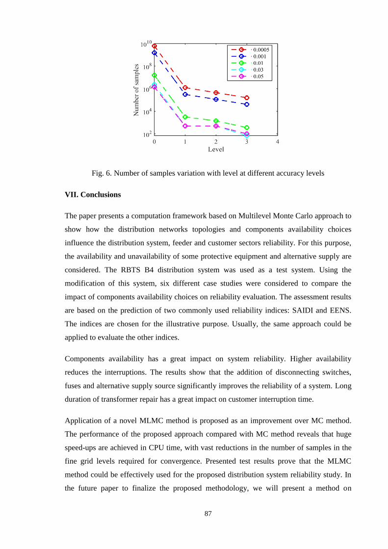
87

Fig. 6. Number of samples variation with level at different accuracy levels

VII. Conclusions

The paper presents a computation framework based on Multilevel Monte Carlo approach to

show how the distribution networks topologies and components availability choices

influence the distribution system, feeder and customer sectors reliability. For this purpose,

the availability and unavailability of some protective equipment and alternative supply are

considered. The RBTS B4 distribution system was used as a test system. Using the

modification of this system, six different case studies were considered to compare the

impact of components availability choices on reliability evaluation. The assessment results

are based on the prediction of two commonly used reliability indices: SAIDI and EENS.

The indices are chosen for the illustrative purpose. Usually, the same approach could be

applied to evaluate the other indices.

Components availability has a great impact on system reliability. Higher availability

reduces the interruptions. The results show that the addition of disconnecting switches,

fuses and alternative supply source significantly improves the reliability of a system. Long

duration of transformer repair has a great impact on customer interruption time.

Application of a novel MLMC method is proposed as an improvement over MC method.

The performance of the proposed approach compared with MC method reveals that huge

speed-ups are achieved in CPU time, with vast reductions in the number of samples in the

fine grid levels required for convergence. Presented test results prove that the MLMC

method could be effectively used for the proposed distribution system reliability study. In

the future paper to finalize the proposed methodology, we will present a method on

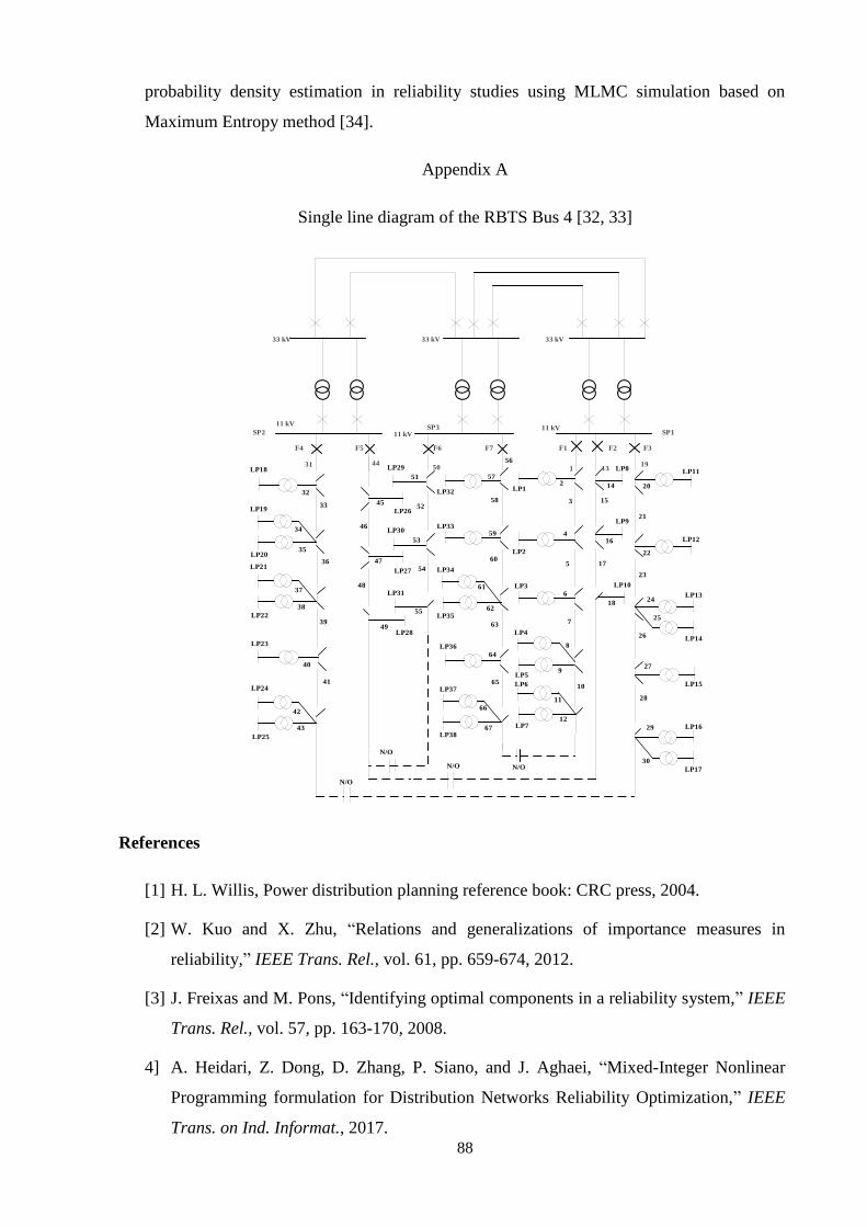
88

probability density estimation in reliability studies using MLMC simulation based on

Maximum Entropy method [34].

Appendix A

Single line diagram of the RBTS Bus 4 [32, 33]

N/O

45

46

47

48

33 kV33 kV33 kV

11 kV11 kV

11 kV

F3F2F1F7F6F5F4

1913150

4431

20

21

22

23

24

25

26

27

28

29

30

14

15

16

17

18

2

3

4

5

6

7

8

9

10

11

12

57

58

59

60

61

62

63

64

65

66

67

51

52

53

54

55

49

32

33

34

35

36

37

38

39

40

41

42

43

LP11

LP12

LP13

LP14

LP15

LP16

LP17

LP8

LP9

LP10

56

LP1

LP2

LP3

LP4

LP5

LP6

LP7

LP32

LP33

LP34

LP35

LP36

LP37

LP38

LP29

LP30

LP31

LP26

LP27

LP28

LP18

LP19

LP20

LP21

LP22

LP23

LP24

LP25

N/O

N/O

N/O

SP1SP2SP3

References

[1] H. L. Willis, Power distribution planning reference book: CRC press, 2004.

[2] W. Kuo and X. Zhu, “Relations and generalizations of importance measures in

reliability,” IEEE Trans. Rel., vol. 61, pp. 659-674, 2012.

[3] J. Freixas and M. Pons, “Identifying optimal components in a reliability system,” IEEE

Trans. Rel., vol. 57, pp. 163-170, 2008.

4] A. Heidari, Z. Dong, D. Zhang, P. Siano, and J. Aghaei, “Mixed-Integer Nonlinear

Programming formulation for Distribution Networks Reliability Optimization,” IEEE

Trans. on Ind. Informat., 2017.

89

[5] W. Li, Risk Assessment of Power Systems: Models, Methods, and Applications, 2005,

IEEE Press/Wiley.

[6] H. Mirsaeedi, A. Fereidunian, S. M. Mohammadi-Hosseininejad, P. Dehghanian, and

H. Lesani, “Long-Term Maintenance Scheduling and Budgeting in Electricity

Distribution Systems Equipped with Automatic Switches,” IEEE Trans. on Ind.

Informat., 2017.

[7] V. Calderaro, V. Lattarulo, A. Piccolo, and P. Siano, “Optimal switch placement by

alliance algorithm for improving microgrids reliability,” IEEE Trans. on Ind. Informat.,

vol. 8, pp. 925-934, 2012.

[8] E. Zio, L. Podofillini, and G. Levitin, “Estimation of the importance measures of multi-

state elements by Monte Carlo simulation,” Rel. Eng. Syst. Safety., vol. 86, pp. 191-

204, 2004.

[9] P. Jirutitijaroen and C. Singh, “Comparison of simulation methods for power system

reliability indexes and their distributions,” IEEE Trans. Power Syst., vol. 23, pp. 486-

493, 2008.

[10] T. J. Dodwell, C. Ketelsen, R. Scheichl, and A. L. Teckentrup, “A hierarchical

multilevel Markov chain Monte Carlo algorithm with applications to uncertainty

quantification in subsurface flow,” SIAM/ASA J. Uncertainty Quantification, vol. 3, pp.

1075-1108, 2015.

[11] R. Billinton and A. Jonnavithula, “Composite system adequacy assessment using

sequential Monte Carlo simulation with variance reduction techniques,” IEE Proc.-

Gener. Transm. Distrib., vol. 144, pp. 1-6, 1997.

[12] C. Singh and J. Mitra, “Composite system reliability evaluation using state space

pruning,” IEEE Trans. Power Syst., vol. 12, pp. 471-479, 1997.

[13] K. Hou, H. Jia, X. Xu, Z. Liu, and Y. Jiang, “A continuous time Markov chain based

sequential analytical approach for composite power system reliability assessment,”

IEEE Trans. Power Syst., vol. 31, pp. 738-748, 2016.


dependent systems via sequential cross-entropy Monte Carlo simulation,” IEEE Trans.

Power Syst., vol. 26, pp. 2381-2389, 2011.

90

[15] Y. Wang, C. Guo, and Q. Wu, “A cross-entropy-based three-stage sequential

importance sampling for composite power system short-term reliability evaluation,”


[16] A. S. N. Huda and R. Zivanovic, “Accelerated distribution systems reliability

evaluation by multilevel monte carlo simulation: implementation of two discretisation

schemes,” IET Gener. Transm. Distrib., vol. 11, pp. 3397-3405, 2017.

[17] A. M. L. da Silva, R. A. Fernandez, and C. Singh, “Generating capacity reliability

evaluation based on Monte Carlo simulation and cross-entropy methods,” IEEE Trans.

Power Syst., vol. 25, pp. 129-137, 2010.

[18] A. M. L. da Silva, R. A. González-Fernández, W. S. Sales, and L. A. Manso,

“Reliability assessment of time-dependent systems via quasi-sequential Monte Carlo

simulation,” in Proc. IEEE 11th Int. Conf. Probabilistic Methods Applied to Power

Systems (PMAPS), 2010, pp. 697-702.

[19] R. González-Fernández and A. L. Da Silva, “Comparison between different cross-

entropy based methods applied to generating capacity reliability,” in Proc. IEEE 12th

Int. Conf. Probabilistic Methods Applied to Power Systems (PMAPS), 2012, pp. 10-14.

[20] A. L. Da Silva, L. D. F. Manso, J. D. O. Mello, and R. Billinton, “Pseudo-

chronological simulation for composite reliability analysis with time varying loads,”


[21] R. A. González-Fernández, A. M. L. da Silva, L. C. Resende, and M. T. Schilling,

“Composite systems reliability evaluation based on Monte Carlo simulation and cross-

entropy methods,” IEEE Trans. Power Syst., vol. 28, pp. 4598-4606, 2013.

[22] E. Tómasson and L. Söder, “Improved Importance Sampling for Reliability

Evaluation of Composite Power Systems,” IEEE Trans. Power Syst., vol. 32, pp. 2426-

2434, 2017.

[23] B. Hua, Z. Bie, S.-K. Au, W. Li, and X. Wang, “Extracting rare failure events in

composite system reliability evaluation via subset simulation,” IEEE Trans. Power

Syst., vol. 30, pp. 753-762, 2015.

[24] G. T. Heydt and T. J. Graf, “Distribution system reliability evaluation using enhanced

samples in a Monte Carlo approach,” IEEE Trans. Power Syst., vol. 25, pp. 2006-2008,

2010.

91

[25] F. Li, “A fast approach of Monte Carlo simulation based on linear contribution factors

to distribution reliability indices,” in Proc. IEEE PES Transmission and Distribution

Conf. and Exposition, 2003, pp. 973-977.

[26] R. Arya, A. Tiwary, S. Choube, and L. Arya, “A smooth bootstrapping based

technique for evaluating distribution system reliability indices neglecting random

interruption duration,” Int. J Electr. Power Energy Syst., vol. 51, pp. 307-310, 2013.

[27] M. B. Giles, “Multilevel monte Carlo path simulation,” Oper. Res., vol. 56, pp. 607-

617, 2008.

[28] M. Giles, “Improved multilevel Monte Carlo convergence using the Milstein scheme,”

in Monte Carlo and quasi-Monte Carlo methods 2006, Springer, 2008, pp. 343-358.

[29] J. M. Harrison, Brownian motion and stochastic flow systems, 1985, Wiley New

York.

[30] B. Oksendal, Stochastic differential equations: an introduction with applications,

2013, Springer Science & Business Media.

[31] R. Billinton and P. Wang, “Teaching distribution system reliability evaluation using

Monte Carlo simulation,” IEEE Trans. Power Syst., vol. 14, pp. 397-403, 1999.

[32] A. S. N. Huda and R. Živanović, “Multilevel Monte Carlo simulation applied to

distribution systems reliability evaluation,” in Proc. IEEE Manchester PowerTech,

2017, pp. 1-6.

[33] R. N. Allan, R. Billinton, I. Sjarief, L. Goel, and K. So, “A reliability test system for

educational purposes-basic distribution system data and results,” IEEE Trans. Power

Syst., vol. 6, pp. 813-820, 1991.

[34] C. Bierig and A. Chernov, “Approximation of probability density functions by the

Multilevel Monte Carlo Maximum Entropy method, ” J. Comput. Phys., vol. 314, pp.

661-681, 2016.

92

Chapter 5

Interrupted Energy Estimation

93


Title of Paper Estimation of Expected Energy Not Supplied considering Time-Varying Load Models by

Multilevel Monte Carlo method: Effect of different factors on computation variation





manuscript style

Publication Details A. S. Nazmul Huda and Rastko Živanović (2018) Estimation of Expected Energy Not Supplied

considering Time-Varying Load Models by Multilevel Monte Carlo method: Effect of different

factors on computation variation, Electric Power Components and Systems (Taylor & Francis).

Revision submitted.

Principal author


(Candidate)

A. S. Nazmul Huda



manuscript.





paper.









Signature

Date 13.08.2018

94

Estimation of Expected Energy Not Supplied considering Time-Varying Load Models

by Multilevel Monte Carlo method: Effect of different factors on computation

variation

Abstract— The paper presents the estimation of power distribution systems Expected

Energy Not Supplied (EENS) index by incorporating Time-Varying Load Models of

different customer sectors. An application of a new and efficient advanced Monte Carlo

simulation (MCS) with controllable accuracy called Multilevel Monte Carlo (MLMC)

method is proposed for this estimation. The purpose of the proposed method is to increase

the simulation speed of EENS estimation. The method could be easily replaced by the

traditional MCS based estimation which requires huge computational effort for achieving

high level of simulation accuracy.

Five distribution networks with seven different load models of Roy Billinton Test

System are chosen as test distribution systems. To verify the effectiveness of the proposed

method, computational time and estimated values of EENS using MLMC method are

compared to the results from MCS. The computation performance of EENS estimation can

be influenced by different factors and criteria which are also explored in this study. The

results presented in the paper show that acceptable results can be obtained using the

proposed method while substantial reduction of computational effort is also achieved.

Keywords— power distribution systems; Expected Energy Not Supplied; Time-Varying

Load Models; Multilevel Monte Carlo simulation; Euler-Maruyama method.

1. Introduction

In distribution systems planning studies, customer expected interrupted energy is referred

as the Expected Energy Not Supplied (EENS) index. Majority of the interruptions

experienced by customers occur due to the distribution system components failures [1].

EENS index provides the information of the expected amount of energy shortage due to the

failures in a specified time period [2, 3]. Based on the accurate estimation of the EENS

index, appropriate planning and design initiatives could be implemented in the distribution

systems for supplying cost-effective and reliable power to customers.

In reliability estimation including EENS estimation, two basic random variables are

present i.e. Time-to-Failure (TTF) and Time-to-Repair (TTR) [4]. TTF is the expected time

for a component to remain in the up state before it fails. TTR of a component is the

95

expected time required for a crew to repair an outage and restore the normal operation of

the system. For accurate estimation, the uncertainties related to these variables are

considered based on probability distribution. The accurate approximation of EENS also

considers the Time-Varying Load Levels (TVLM) of different customer sectors such as

residential, industrial and commercial, etc. Load level of a specific customer type usually

fluctuates due to the discrepancy of the hourly load consumption level throughout a 24-

hour period. In addition, seasonal inconsistency in the weather contributes prominently to

loading level diversity [5].

For distribution system EENS estimation, two approaches are generally utilized, i.e.

analytical and simulation approaches [6, 7]. Analytical approach calculates EENS by

considering the constant specified values of random variables. On the other hand,

simulation method mainly based on sequential Monte Carlo simulation (MCS) estimates

the EENS by considering the probability distributions of these random variables which

requires a large number of iterations depending on the target accuracy level, especially

while dealing with the rare events [8]. Therefore, MCS is usually a time-consuming

method. To increase the computational speed of MCS, numerous advanced MCS methods

have been studied for power systems planning applications [9-12]. However, a small

number of relevant studies have been conducted for distribution systems planning [13-15].

The review also shows that the result of system EENS estimation with the uncertainties of

TTF and TTR through incorporating TVLM using any advanced MCS method has not

been reported yet. For this reason, the novel application of an advanced MCS method

called the Multilevel Monte Carlo (MLMC) simulation has been implemented and tested in

this study in order to accelerate estimation process.

The MLMC method was first introduced by Heinrich for parametric integration [16] and

then Giles extended the idea to the simulation of the stochastic process [17]. The

fundamental improvement of the MLMC method is to utilize a hierarchy of discretisation

levels and estimate expected value of a quantity of interest from a weighted sum of

expectations over those levels. The optimized number of samples on each level is

generated to run most of the simulations on the coarser levels with inexpensive forward

computations. On the other hand, fewer samples are run on the more expensive finer

resolution scales because of the smaller variances. By this approach, the MLMC method

produces an unbiased estimator providing acceptable accuracy with considerably reduced

computational effort than original MCS.

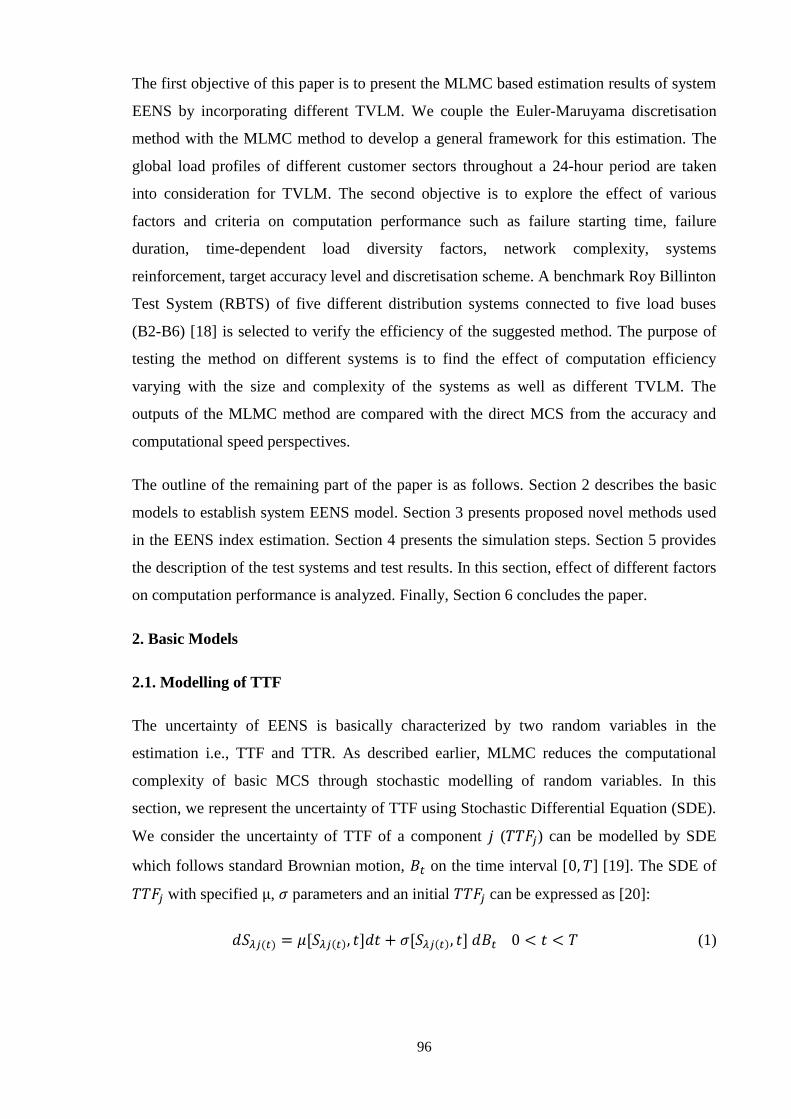
96

The first objective of this paper is to present the MLMC based estimation results of system

EENS by incorporating different TVLM. We couple the Euler-Maruyama discretisation

method with the MLMC method to develop a general framework for this estimation. The

global load profiles of different customer sectors throughout a 24-hour period are taken

into consideration for TVLM. The second objective is to explore the effect of various

factors and criteria on computation performance such as failure starting time, failure

duration, time-dependent load diversity factors, network complexity, systems

reinforcement, target accuracy level and discretisation scheme. A benchmark Roy Billinton

Test System (RBTS) of five different distribution systems connected to five load buses

(B2-B6) [18] is selected to verify the efficiency of the suggested method. The purpose of

testing the method on different systems is to find the effect of computation efficiency

varying with the size and complexity of the systems as well as different TVLM. The

outputs of the MLMC method are compared with the direct MCS from the accuracy and

computational speed perspectives.

The outline of the remaining part of the paper is as follows. Section 2 describes the basic

models to establish system EENS model. Section 3 presents proposed novel methods used

in the EENS index estimation. Section 4 presents the simulation steps. Section 5 provides

the description of the test systems and test results. In this section, effect of different factors

on computation performance is analyzed. Finally, Section 6 concludes the paper.

2. Basic Models

2.1. Modelling of TTF

The uncertainty of EENS is basically characterized by two random variables in the

estimation i.e., TTF and TTR. As described earlier, MLMC reduces the computational

complexity of basic MCS through stochastic modelling of random variables. In this

section, we represent the uncertainty of TTF using Stochastic Differential Equation (SDE).

We consider the uncertainty of TTF of a component ( ) can be modelled by SDE

which follows standard Brownian motion, on the time interval [ ] [19]. The SDE of

with specified , parameters and an initial can be expressed as [20]:

(1)

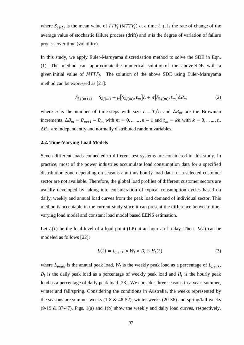
97

where is the mean value of ( at a time , is the rate of change of the

average value of stochastic failure process (drift) and is the degree of variation of failure

process over time (volatility).

In this study, we apply Euler-Maruyama discretisation method to solve the SDE in Eqn.

(1). The method can approximate the numerical solution of the above SDE with a

given initial value of . The solution of the above SDE using Euler-Maruyama

method can be expressed as [21]:

(2)

where is the number of time-steps with size and are the Brownian

increments. with and with .

are independently and normally distributed random variables.

2.2. Time-Varying Load Models

Seven different loads connected to different test systems are considered in this study. In

practice, most of the power industries accumulate load consumption data for a specified

distribution zone depending on seasons and thus hourly load data for a selected customer

sector are not available. Therefore, the global load profiles of different customer sectors are

usually developed by taking into consideration of typical consumption cycles based on

daily, weekly and annual load curves from the peak load demand of individual sector. This

method is acceptable in the current study since it can present the difference between time-

varying load model and constant load model based EENS estimation.

Let be the load level of a load point (LP) at an hour of a day. Then can be

modeled as follows [22]:

(3)

where is the annual peak load, is the weekly peak load as a percentage of ,

is the daily peak load as a percentage of weekly peak load and is the hourly peak

load as a percentage of daily peak load [23]. We consider three seasons in a year: summer,

winter and fall/spring. Considering the conditions in Australia, the weeks represented by

the seasons are summer weeks (1-8 & 48-52), winter weeks (20-36) and spring/fall weeks

(9-19 & 37-47). Figs. 1(a) and 1(b) show the weekly and daily load curves, respectively.

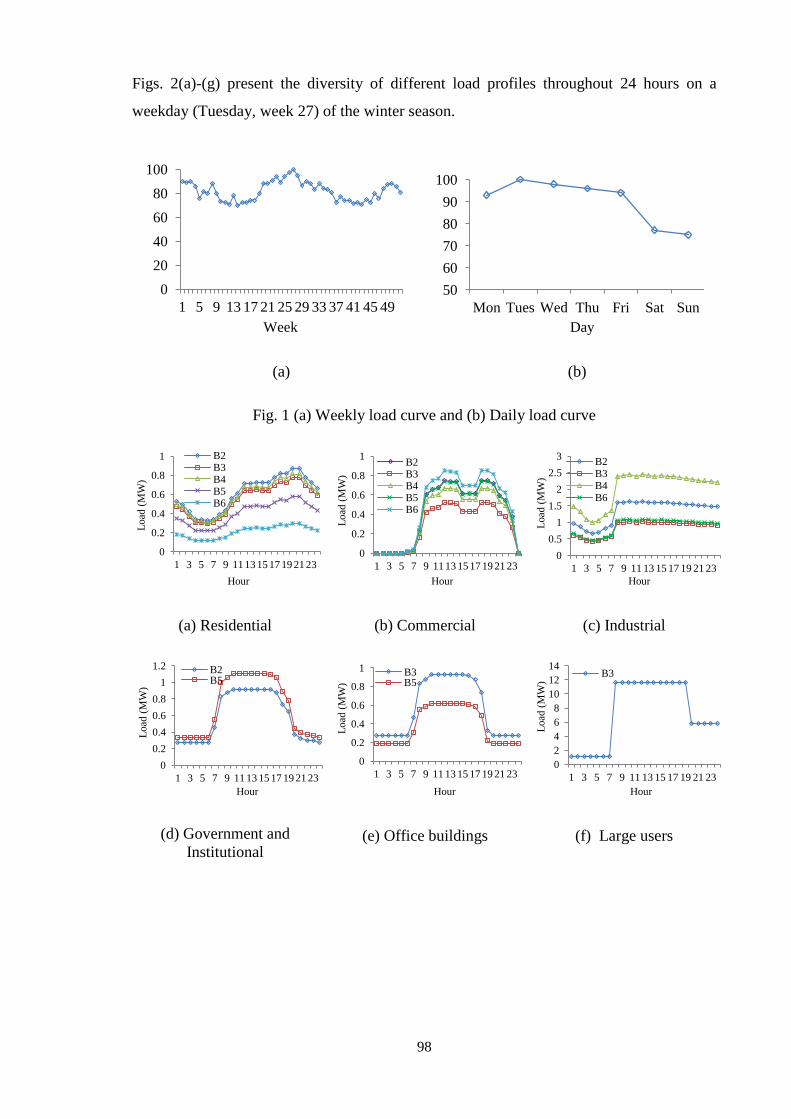
98

Figs. 2(a)-(g) present the diversity of different load profiles throughout 24 hours on a

weekday (Tuesday, week 27) of the winter season.

(a)

(b)

Fig. 1 (a) Weekly load curve and (b) Daily load curve

(a) Residential

(b) Commercial

(c) Industrial

(d) Government and

Institutional

(e) Office buildings

(f) Large users

0

20

40

60

80

100

1 5 9 13 17 21 25 29 33 37 41 45 49

Week

50

60

70

80

90

100

Mon Tues Wed Thu Fri Sat Sun

Day

0

0.2

0.4

0.6

0.8

1

1 3 5 7 9 11 13 15 17 19 21 23

Load

(M

W)

Hour

B2 B3 B4 B5 B6

0

0.2

0.4

0.6

0.8

1

1 3 5 7 9 11 13 15 17 19 21 23

Load

(M

W)

Hour

B2 B3 B4 B5 B6

0

0.5

1

1.5

2

2.5

3

1 3 5 7 9 11 13 15 17 19 21 23

Load

(M

W)

Hour

B2 B3 B4 B6

0

0.2

0.4

0.6

0.8

1

1.2

1 3 5 7 9 11 13 15 17 19 21 23

Load

(M

W)

Hour

B2 B5

0

0.2

0.4

0.6

0.8

1

1 3 5 7 9 11 13 15 17 19 21 23

Load

(M

W)

Hour

B3 B5

0

2

4

6

8

10

12

14

1 3 5 7 9 11 13 15 17 19 21 23

Load

(M

W)

Hour

B3

99

(g) Agricultural

Fig. 2. Daily load profile for different loads of distribution systems

3. MCS and MLMC method

3.1. MCS method

The standard MCS estimator using number of independent samples is as follows [17]:

(4)

where

is the ith sample of . is the EENS value of a distribution system. The

expected value of the estimator is and it is simulated on a finest level . is a

nonnegative integer. The accuracy and computational burden of the estimation on this level

are very high. The variance of the above estimator is . It requires

samples for an accuracy of ( is the root mean square error) and computational burden is

increased with the increase of target accuracy level.

3.2. MLMC method

The following sections describe how EENS evaluation estimators are constructed using

MLMC method and then how the estimators satisfy the convergence condition.

3.2.1. Construct of MLMC estimator

The MLMC method is a variance reduction technique for the MCS. In this method, the

system EENS is estimated using MCS with multiple time-step sizes defined as

as of Eqn. (2). Here with being the computationally low-cost

coarsest level and being the most expensive finest level. The fine and coarse

estimators are calculated using time-step of and ,

0

0.1

0.2

0.3

0.4

1 3 5 7 9 11 13 15 17 19 21 23

Load

(M

W)

Hour

B6

100

respectively. The MLMC estimator is calculated as a sum of level MCS estimator

corrections as follows:

(5)

where is the number of samples on each level .

The expected value of the MLMC estimator can be written as

(6)

The unbiased estimator of the term is as follows:

(7)

The estimator for the can be calculated as:

(8)

A geometric sequence of time-steps is used in the MLMC method as Eqn. (6) and therefore

less accurate estimation on a level can be consecutively corrected by the subsequent fine

levels estimations. This ensures the same value of EENS in the MLMC method as MCS. In

addition, both coarse and fine estimators are calculated as

to avoid

undesired bias introduction and therefore,

. (9)

3.2.2. Testing MLMC convergence

The accuracy of the MLMC estimator can be expressed as:

(10)

where the variance of the MLMC estimator is

.

The first and second terms in Eqn. (10) are the sampling error and bias error, respectively.

In order to ensure accuracy of the MLMC estimator is less than , it is adequate to

confirm that both sampling and bias errors are less than . If is the computational

cost of one sample of , then the total expected cost of the MLMC estimator is

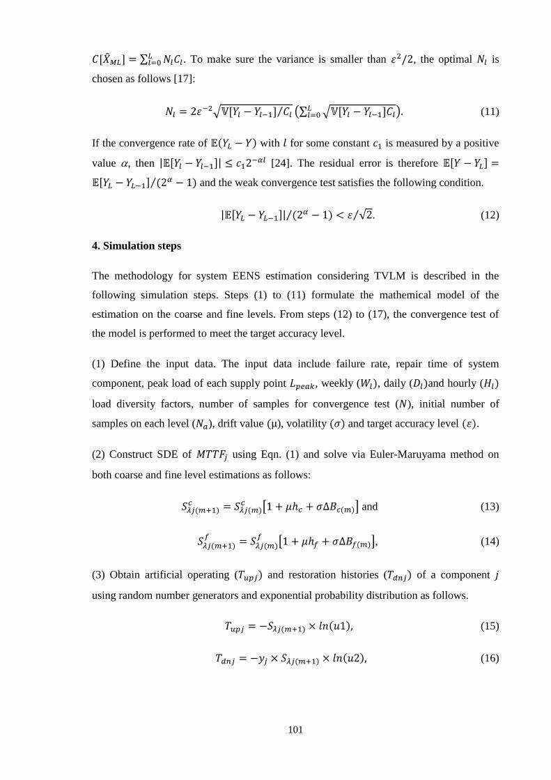
101

. To make sure the variance is smaller than , the optimal is

chosen as follows [17]:

(11)

If the convergence rate of with for some constant is measured by a positive

value , then [24]. The residual error is therefore

and the weak convergence test satisfies the following condition.

. (12)

4. Simulation steps

The methodology for system EENS estimation considering TVLM is described in the

following simulation steps. Steps (1) to (11) formulate the mathemical model of the

estimation on the coarse and fine levels. From steps (12) to (17), the convergence test of

the model is performed to meet the target accuracy level.

(1) Define the input data. The input data include failure rate, repair time of system

component, peak load of each supply point , weekly ( , daily ( and hourly (

load diversity factors, number of samples for convergence test ( ), initial number of

samples on each level ( ), drift value ), volatility and target accuracy level .

(2) Construct SDE of using Eqn. (1) and solve via Euler-Maruyama method on

both coarse and fine level estimations as follows:

and (13)

, (14)

(3) Obtain artificial operating ( and restoration histories ( of a component

using random number generators and exponential probability distribution as follows.

(15)

(16)

102

where is a constant for component and . and are the average failure

rate and mean TTR of component , respectively. and are uniformly distributed

random variables between [0,1].

(4) Calculate annual unavailability, (hr/yr) of component on both levels as follows:

(17)

where N is the desired number of simulated periods.

(5) Repeat the steps (2)-(4) for each distribution system component failure.

(6) Find the LPs affected by component failure.

(7) Calculate annual unavailability, of a load point ( ) on both levels by using sum

of the unavailability values of all components connected to the .

(18)

where is the number of components failure that interrupt the service of .

(8) Find the possible load profile for based on Eqn. (3) during the outage period and

calculate the average load level during this period.

(19)

where and are failure start and end hour, respectively.

(9) Repeat the steps (2)-(8) for each LP in the system.

(10) Estimate the expected value of system EENS as follows.

(20)

where is the number of LPs in the system.

(11) Calculate the sum of the system EENS values of levels and . The

simulation is repeated until the number of samples is reached to .

(12) Set the initial finest level of MLMC simulation as .

103

(13) Generate number of samples on each using and also update step

(11).

(14) Calculate the absolute mean of EENS and variance on each level .

(15) Find out the optimal number of samples on each level using Eqn. (11) and evaluate

extra samples if needed by comparing with . Moreover, update mean and variance on

each level for confirming variance of the MLMC estimator

(16) Test weak convergence using Eqn. (12). If not converged, set and repeat

from step (13) until reached to the target accuracy level.

(17) Finally calculate the multilevel estimator by Eqn. (6).

5. Test systems and results

5.1. Test systems

Five radial distribution systems connected to five different load buses (bus 2-bus 6) of a

benchmark RBTS are considered as test systems. The single line diagrams of the test

systems are given in [18]. Table 1 shows the information of the load types, number of

feeders and load points (LPs) in the distribution systems. The RBTS connected to B2-B5

represent the typical urban systems. The distribution system for B6 represents a typical

rural type network. The amount of load consumption may differ from system to system due

to the mix and dispersion of customer served. The peak load contribution of different loads

in the test systems is also shown in Table 1. The large users and office building users

sectors of RBTS B3 system have the highest and lowest percentage of peak load with

65.29% and 2.18%, respectively. The residential load type of all test systems except RBTS

B3 contributes highest percentage of peak load. The agricultural load is only available in

RBTS B6 system and makes contribution of 37% of total peak load. Some systems contain

multiple kinds of the same load with dissimilar peak load connected to different LPs. For

example, in RBTS B2 system, there are two types of residential load. Some residential LPs

(1-3, 10, 11) have peak load of 0.8668 MW. On the other hand, few LPs (12, 17-19) have

peak load of 0.7291 MW.

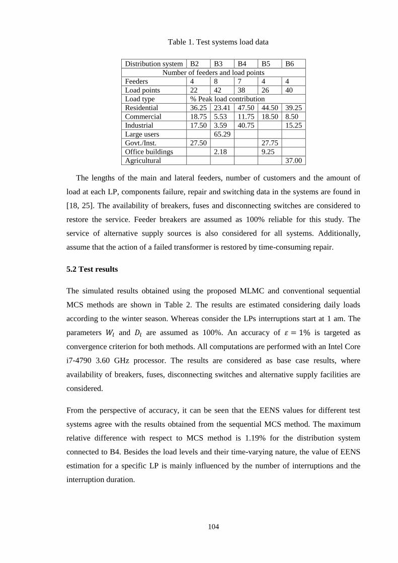
104

Table 1. Test systems load data

Distribution system B2 B3 B4 B5 B6

Number of feeders and load points

Feeders 4 8 7 4 4

Load points 22 42 38 26 40

Load type % Peak load contribution

Residential 36.25 23.41 47.50 44.50 39.25

Commercial 18.75 5.53 11.75 18.50 8.50

Industrial 17.50 3.59 40.75 15.25

Large users 65.29

Govt./Inst. 27.50 27.75

Office buildings 2.18 9.25

Agricultural 37.00

The lengths of the main and lateral feeders, number of customers and the amount of

load at each LP, components failure, repair and switching data in the systems are found in

[18, 25]. The availability of breakers, fuses and disconnecting switches are considered to

restore the service. Feeder breakers are assumed as 100% reliable for this study. The

service of alternative supply sources is also considered for all systems. Additionally,

assume that the action of a failed transformer is restored by time-consuming repair.

5.2 Test results

The simulated results obtained using the proposed MLMC and conventional sequential

MCS methods are shown in Table 2. The results are estimated considering daily loads

according to the winter season. Whereas consider the LPs interruptions start at 1 am. The

parameters and are assumed as 100%. An accuracy of is targeted as

convergence criterion for both methods. All computations are performed with an Intel Core

i7‐4790 3.60 GHz processor. The results are considered as base case results, where

availability of breakers, fuses, disconnecting switches and alternative supply facilities are

considered.

From the perspective of accuracy, it can be seen that the EENS values for different test

systems agree with the results obtained from the sequential MCS method. The maximum

relative difference with respect to MCS method is 1.19% for the distribution system

connected to B4. Besides the load levels and their time-varying nature, the value of EENS

estimation for a specific LP is mainly influenced by the number of interruptions and the

interruption duration.

105

Table 2. Base case EENS estimation results


EENS (MCS) 35.42 48.21 43.55 43.48 42.40

EENS (MLMC) 36.20 48.76 44.07 43.90 42.82

Relative Errors (%) 1.06 1.14 1.19 0.96 0.99

MCS time (s) 22.08 38.26 32.47 35.93 40.64

MLMC time (s) 1.08 1.91 1.52 1.73 1.96

Speedup (MCS/MLMC) 20.44 20.03 21.36 20.76 20.73

From the computational speed perspective, the proposed method saves a huge time for all

the systems as shown in Table 2. For example, the sequential simulation approach utilizes

32.93 seconds (s) of CPU time for B4 system whereas the method with multilevel

approach uses only 1.52 s, i.e., an increase of 20.44 times in the computational speed is

attained. In all the cases, the percentage of computation speedup is above 90%. MLMC

method reduces the computational effort of MCS method by reducing the number of

samples on the finest level. For RBTS B4, the proposed method uses 1638 samples on the

finest level and the MCS requires 10750 samples for convergence. Due to the utilization of

many samples, MCS method estimates EENS with noticeably high accuracy compared to

MLMC method.

The effects of different factors on EENS estimation performance are discussed in the

following.

5.2.1. Effect of failure starting time

The starting time of a LP failure influences greatly the estimation of system EENS and its

computation time. A very straightforward way to compute EENS is to use constant load

level (Average) of a specific load point. Fig. 3 shows the difference between EENS results

based on time-varying and constant load models (Avg) for different test systems. Three

different starting times including peak and off-peak hours are considered to evaluate the

effect of failure starting time (FST) on this estimation. It can be clearly seen that EENS

values vary with the FST and there is a significant difference when compared to constant

load model based EENS. At a.m., due to the high percentage of for almost all

load types during this period, test systems achieve overall maximum EENS than others

except RBTS B6. In RBTS B6, there are four different types of LPs. From these,

residential and agricultural load models contribute 39.25% and 37% of total peak load,

respectively. From the Figs. 2(a) and 2(g), it is seen that both loads add high percentage of

during the failure period starting at FST= 4 p.m. which supplies maximum EENS for

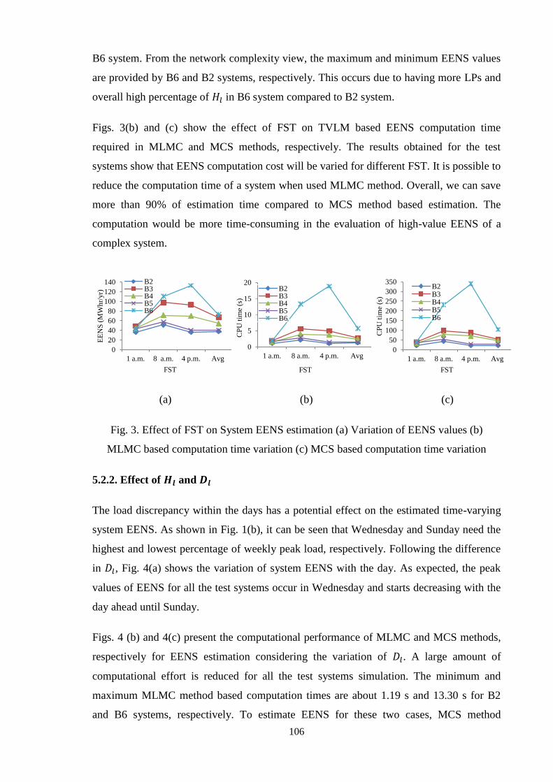
106

B6 system. From the network complexity view, the maximum and minimum EENS values

are provided by B6 and B2 systems, respectively. This occurs due to having more LPs and

overall high percentage of in B6 system compared to B2 system.

Figs. 3(b) and (c) show the effect of FST on TVLM based EENS computation time

required in MLMC and MCS methods, respectively. The results obtained for the test

systems show that EENS computation cost will be varied for different FST. It is possible to

reduce the computation time of a system when used MLMC method. Overall, we can save

more than 90% of estimation time compared to MCS method based estimation. The

computation would be more time-consuming in the evaluation of high-value EENS of a

complex system.

(a)

(b)

(c)

Fig. 3. Effect of FST on System EENS estimation (a) Variation of EENS values (b)

MLMC based computation time variation (c) MCS based computation time variation

5.2.2. Effect of and

The load discrepancy within the days has a potential effect on the estimated time-varying

system EENS. As shown in Fig. 1(b), it can be seen that Wednesday and Sunday need the

highest and lowest percentage of weekly peak load, respectively. Following the difference

in , Fig. 4(a) shows the variation of system EENS with the day. As expected, the peak

values of EENS for all the test systems occur in Wednesday and starts decreasing with the

day ahead until Sunday.

Figs. 4 (b) and 4(c) present the computational performance of MLMC and MCS methods,

respectively for EENS estimation considering the variation of . A large amount of

computational effort is reduced for all the test systems simulation. The minimum and

maximum MLMC method based computation times are about 1.19 s and 13.30 s for B2

and B6 systems, respectively. To estimate EENS for these two cases, MCS method

0

20

40

60

80

100

120

140

1 a.m. 8 a.m. 4 p.m. Avg

EE

NS

(M

Wh

r/yr)

FST

B2 B3 B4 B5 B6

0

5

10

15

20

1 a.m. 8 a.m. 4 p.m. Avg

CP

U t

ime

(s)

FST

B2 B3 B4 B5 B6

0

50

100

150

200

250

300

350

1 a.m. 8 a.m. 4 p.m. Avg

CP

U t

ime

(s)

FST

B2 B3 B4 B5 B6

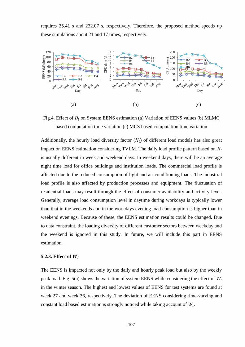
107

requires 25.41 s and 232.07 s, respectively. Therefore, the proposed method speeds up

these simulations about 21 and 17 times, respectively.

(a)

(b)

(c)

Fig.4. Effect of on System EENS estimation (a) Variation of EENS values (b) MLMC

based computation time variation (c) MCS based computation time variation

Additionally, the hourly load diversity factor ( ) of different load models has also great

impact on EENS estimation considering TVLM. The daily load profile pattern based on

is usually different in week and weekend days. In weekend days, there will be an average

night time load for office buildings and institution loads. The commercial load profile is

affected due to the reduced consumption of light and air conditioning loads. The industrial

load profile is also affected by production processes and equipment. The fluctuation of

residential loads may result through the effect of consumer availability and activity level.

Generally, average load consumption level in daytime during workdays is typically lower

than that in the weekends and in the workdays evening load consumption is higher than in

weekend evenings. Because of these, the EENS estimation results could be changed. Due

to data constraint, the loading diversity of different customer sectors between weekday and

the weekend is ignored in this study. In future, we will include this part in EENS

estimation.

5.2.3. Effect of

The EENS is impacted not only by the daily and hourly peak load but also by the weekly

peak load. Fig. 5(a) shows the variation of system EENS while considering the effect of

in the winter season. The highest and lowest values of EENS for test systems are found at

week 27 and week 36, respectively. The deviation of EENS considering time-varying and

constant load based estimation is strongly noticed while taking account of .

0

20

40

60

80

100

120

EE

NS

(M

Wh

r/yr)

Day

B2 B3 B4 B5 B6 0

2

4

6

8

10

12

14

CP

U t

ime

(s)

Day

B2 B3 B4 B5 B6

0

50

100

150

200

250

CP

U t

ime

(s)

Day

B2 B3 B4 B5 B6

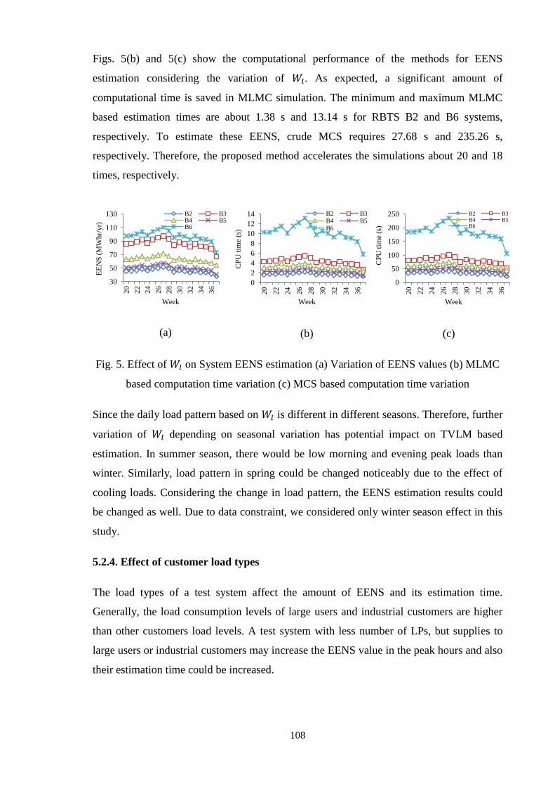
108

Figs. 5(b) and 5(c) show the computational performance of the methods for EENS

estimation considering the variation of . As expected, a significant amount of

computational time is saved in MLMC simulation. The minimum and maximum MLMC

based estimation times are about 1.38 s and 13.14 s for RBTS B2 and B6 systems,

respectively. To estimate these EENS, crude MCS requires 27.68 s and 235.26 s,

respectively. Therefore, the proposed method accelerates the simulations about 20 and 18

times, respectively.

(a)

(b)

(c)

Fig. 5. Effect of on System EENS estimation (a) Variation of EENS values (b) MLMC

based computation time variation (c) MCS based computation time variation

Since the daily load pattern based on is different in different seasons. Therefore, further

variation of depending on seasonal variation has potential impact on TVLM based

estimation. In summer season, there would be low morning and evening peak loads than

winter. Similarly, load pattern in spring could be changed noticeably due to the effect of

cooling loads. Considering the change in load pattern, the EENS estimation results could

be changed as well. Due to data constraint, we considered only winter season effect in this

study.

5.2.4. Effect of customer load types

The load types of a test system affect the amount of EENS and its estimation time.

Generally, the load consumption levels of large users and industrial customers are higher

than other customers load levels. A test system with less number of LPs, but supplies to

large users or industrial customers may increase the EENS value in the peak hours and also

their estimation time could be increased.

30

50

70

90

110

130

20

22

24

26

28

30

32

34

36

EE

NS

(M

Wh

r/yr)

Week

B2 B3 B4 B5 B6

0

2

4

6

8

10

12

14

20

22

24

26

28

30

32

34

36

CP

U t

ime

(s)

Week

B2 B3 B4 B5 B6

0

50

100

150

200

250

20

22

24

26

28

30

32

34

36

CP

U t

ime

(s)

Week

B2 B3 B4 B5 B6

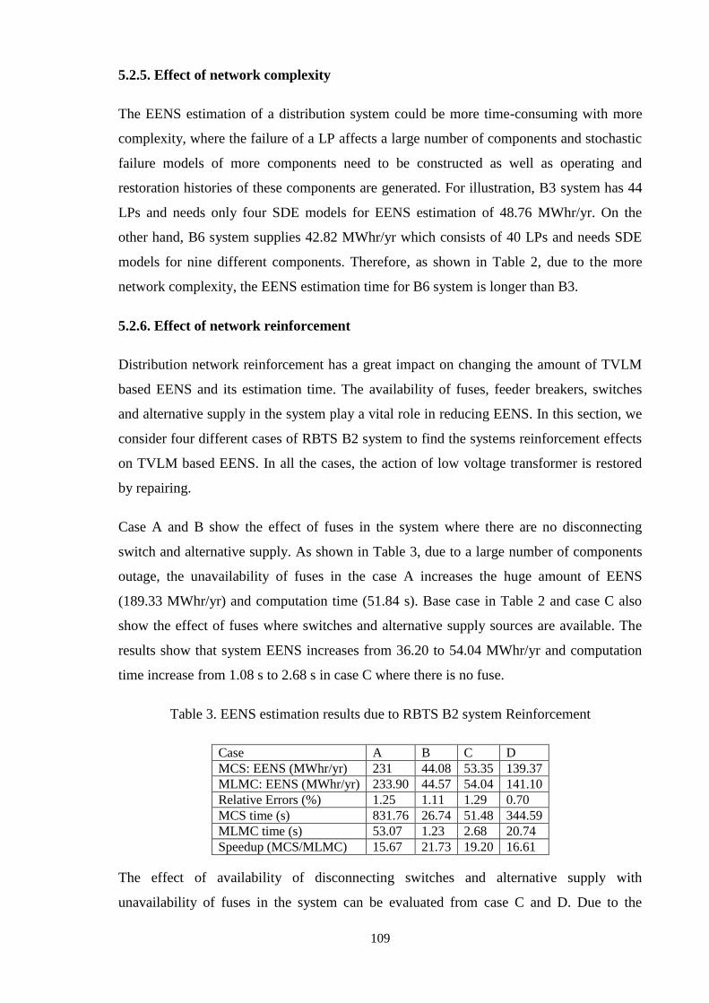
109

5.2.5. Effect of network complexity

The EENS estimation of a distribution system could be more time-consuming with more

complexity, where the failure of a LP affects a large number of components and stochastic

failure models of more components need to be constructed as well as operating and

restoration histories of these components are generated. For illustration, B3 system has 44

LPs and needs only four SDE models for EENS estimation of 48.76 MWhr/yr. On the

other hand, B6 system supplies 42.82 MWhr/yr which consists of 40 LPs and needs SDE

models for nine different components. Therefore, as shown in Table 2, due to the more

network complexity, the EENS estimation time for B6 system is longer than B3.

5.2.6. Effect of network reinforcement

Distribution network reinforcement has a great impact on changing the amount of TVLM

based EENS and its estimation time. The availability of fuses, feeder breakers, switches

and alternative supply in the system play a vital role in reducing EENS. In this section, we

consider four different cases of RBTS B2 system to find the systems reinforcement effects

on TVLM based EENS. In all the cases, the action of low voltage transformer is restored

by repairing.

Case A and B show the effect of fuses in the system where there are no disconnecting

switch and alternative supply. As shown in Table 3, due to a large number of components

outage, the unavailability of fuses in the case A increases the huge amount of EENS

(189.33 MWhr/yr) and computation time (51.84 s). Base case in Table 2 and case C also

show the effect of fuses where switches and alternative supply sources are available. The

results show that system EENS increases from 36.20 to 54.04 MWhr/yr and computation

time increase from 1.08 s to 2.68 s in case C where there is no fuse.

Table 3. EENS estimation results due to RBTS B2 system Reinforcement

Case A B C D

MCS: EENS (MWhr/yr) 231 44.08 53.35 139.37

MLMC: EENS (MWhr/yr) 233.90 44.57 54.04 141.10

Relative Errors (%) 1.25 1.11 1.29 0.70

MCS time (s) 831.76 26.74 51.48 344.59

MLMC time (s) 53.07 1.23 2.68 20.74

Speedup (MCS/MLMC) 15.67 21.73 19.20 16.61

The effect of availability of disconnecting switches and alternative supply with

unavailability of fuses in the system can be evaluated from case C and D. Due to the

110

presence of alternative sources, a total EENS of 87.06 MWhr/yr and computation time of

18.06 s are decreased in case C when compared to case D. Similarly, the effect of

disconnecting switches where there are no fuses and alternative supply sources in the

system can be found from case A and D. The availability of switches in case D can reduce

EENS from 233.90 to 139.37 MWhr/yr and simulation time from 53.07 s to 20.74 s.

5.2.7. Effect of target accuracy level

A higher level of expected accuracy increases the TVLM based estimation time of EENS

as well as decreases the level of variance. Consequently, confidence intervals for the output

EENS become narrower. By comparing with the base case from Table 2, it can be seen

from Table 4 that the increased accuracy level = 0.1% increases huge computational

effort for all test systems.

Table 4. EENS estimation results considering = 0.1%


MCS: EENS (MWhr/yr) 35.81 48.20 43.55 43.47 42.39

MLMC: EENS (MWhr/yr) 36.27 48.80 44.09 44.01 42.92

Relative Errors (%) 1.28 1.24 1.23 1.24 1.25

MCS time (s) 27.79 47.67 38.81 42.44 47.97

MLMC time (s) 1.75 3.26 2.56 2.81 3.27

Speedup (MCS/MLMC) 15.88 14.62 15.16 15.10 14.66

5.2.8. Effect of discretisation scheme

The computational performance of TVLM based EENS estimation can also be affected by

the selection of discretisation scheme for SDE solution. Table 5 shows the estimation

results based on Milstein discretisation method [26]. By comparing between Table 2 and 5,

it can be concluded that estimation based on Milstein method takes less CPU time than that

used by Euler-Maruyama method. Also, the estimation is more accelerated using Milstein

method than Euler-Maruyama method based estimation when compared to basic MCS

method.

Table 5. EENS estimation results based on Milstein method


EENS (MCS) 35.82 48.20 43.55 43.46 42.40

EENS (MLMC) 36.24 48.74 44.10 43.90 42.89

Relative Errors (%) 1.17 1.12 1.26 1.01 1.15

MCS time (s) 25.09 42.01 34.09 38.93 45.53

MLMC time (s) 1.00 1.88 1.58 1.64 1.94

Speedup (MCS/MLMC) 25.09 22.34 21.57 23.73 23.46

111

6. Conclusions

In this paper, a general framework for estimating distribution systems average Expected

Energy Not Supplied (EENS) index considering Time-Varying Load Models has been

proposed based on a novel Multilevel Monte Carlo (MLMC) method. The proposed

method coupled with the Euler-Maruyama discretisation scheme can effectively estimate

the EENS with acceptable accuracy and huge computational time saving compared to the

standard Monte Carlo simulation. The simulation is based on computing the system EENS

using a hierarchy of discretisation levels and estimating the final output by combining

results from different levels. Mean square error considering both sampling and bias errors

is used as the convergence criterion which can be reached by controlling the number of

samples on each level and number of discretisation levels.

Using MLMC method, there is not much difference from the basic concept of EENS

estimation based on constant load models except incorporating time-varying loads in the

estimation. The global load profiles of different customer sectors throughout a 24-hour

period are taken into consideration for this purpose. However, the effect of different

parameters and criteria can significantly change the computation performance of the

MLMC method. The effect of failure starting time, weekly, daily and hourly diversity

factors show a considerable impact on the estimation. The effect of distribution systems

reinforcement shows that unavailability of disconnecting switches, fuses and alternative

supply sources in the systems can increase the amount of EENS and it has a huge impact

on computation effort. Similarly, smaller target accuracy level can increase the estimation

time. The discretisation scheme has also impact on computational performance and

Milstein method can converge faster than Euler-Maruyama method for the EENS

estimation.

In distribution system, integration of renewable energy sources is becoming widespread to

increase the system reliability. Various loads and system random variables [27] could be

modelled using probability distributions. As large numbers of uncertain variables are being

incorporated, maintaining accuracy with reliable convergence speed will become more

challenging in future. Computation method like MLMC can be used for improving system

performance as well as for collecting information of probabilities [28].

112

List of symbols and abbreviations

Average failure rate of a component (given)

Average repair time of a component (given)

Average load level for load point during failure period

Annual peak load

Annual unavailability of component (simulated)

Annual unavailability of a load point (simulated)

Artificial operating history of component

Artificial restoration history of component

Big O notation

Brownian increments

Brownian motion

Coarse path estimator

Computational cost of one sample of Daily peak load as a percentage of weekly peak load

σ Degree of variation of failure process over time

Estimation of expectation on level l

Each grid level

EENS value of a distribution system

EENS value on level Expected cost of the MLMC estimator

EENS Expected Energy Not Supplied

Expected value of the MLMC estimator

Expected value of the MLMC estimator on level

Expected value of the MLMC estimator on coarse level

Expected value of the MLMC estimator on fine level

Failure start hour

Failure end hour

FST Failure starting time

Fine path estimator

Finest level

Hourly peak load as a percentage of daily peak load

ith sample of

Initial number of samples on each level Load point

load point Load level of a LP at an hour t

Mean value of at a time



MLMC Multilevel Monte Carlo

MLMC estimator

Number of components failure that interrupt the service of

Number of load points in the distribution system

Number of Monte Carlo samples

Number of samples for MLMC convergence test

Number of samples on each level Number of samples on each level determined using

Number of time-steps

µ Rate of change of the average value of stochastic failure process

Rate of convergence

Specified accuracy level

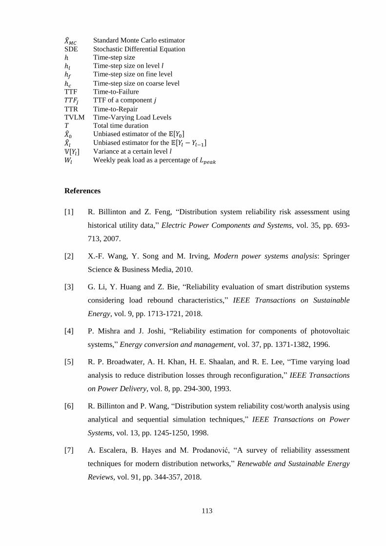
113

Standard Monte Carlo estimator

SDE Stochastic Differential Equation

Time-step size

Time-step size on level l

Time-step size on fine level

Time-step size on coarse level

TTF Time-to-Failure

TTF of a component

TTR Time-to-Repair

TVLM Time-Varying Load Levels

T Total time duration

Unbiased estimator of the

Unbiased estimator for the Variance at a certain level l

Weekly peak load as a percentage of

References

[1] R. Billinton and Z. Feng, “Distribution system reliability risk assessment using

historical utility data,” Electric Power Components and Systems, vol. 35, pp. 693-

713, 2007.

[2] X.-F. Wang, Y. Song and M. Irving, Modern power systems analysis: Springer

Science & Business Media, 2010.

[3] G. Li, Y. Huang and Z. Bie, “Reliability evaluation of smart distribution systems

considering load rebound characteristics,” IEEE Transactions on Sustainable

Energy, vol. 9, pp. 1713-1721, 2018.

[4] P. Mishra and J. Joshi, “Reliability estimation for components of photovoltaic

systems,” Energy conversion and management, vol. 37, pp. 1371-1382, 1996.

[5] R. P. Broadwater, A. H. Khan, H. E. Shaalan, and R. E. Lee, “Time varying load

analysis to reduce distribution losses through reconfiguration,” IEEE Transactions

on Power Delivery, vol. 8, pp. 294-300, 1993.

[6] R. Billinton and P. Wang, “Distribution system reliability cost/worth analysis using

analytical and sequential simulation techniques,” IEEE Transactions on Power

Systems, vol. 13, pp. 1245-1250, 1998.

[7] A. Escalera, B. Hayes and M. Prodanović, “A survey of reliability assessment

techniques for modern distribution networks,” Renewable and Sustainable Energy

Reviews, vol. 91, pp. 344-357, 2018.

114

[8] A. Sankarakrishnan and R. Billinton, “Sequential Monte Carlo simulation for

composite power system reliability analysis with time varying loads,” IEEE



dependent systems via sequential cross-entropy Monte Carlo simulation,” IEEE


[10] K. Hou, H. Jia, X. Xu, Z. Liu, and Y. Jiang, “A continuous time Markov chain

based sequential analytical approach for composite power system reliability

assessment,” IEEE Transactions on Power Systems, vol. 31, pp. 738-748, 2016.

[11] R. Billinton, L. Cui, Z. Pan, and P. Wang, “Probability distribution development in

distribution system reliability evaluation,” Electric Power Components and

Systems, vol. 30, pp. 907-916, 2002.

[12] E. Tomasson and L. Söder, “Improved importance sampling for reliability

evaluation of composite power systems,” IEEE Transactions on Power Systems,

vol. 32, pp. 2426-2434, 2017.

[13] F. Li, “A fast approach of Monte Carlo simulation based on linear contribution

factors to distribution reliability indices,” in Transmission and Distribution

Conference and Exposition, 2003 IEEE PES, 2003, pp. 973-977.

[14] G. T. Heydt and T. J. Graf, “Distribution system reliability evaluation using

enhanced samples in a Monte Carlo approach,” IEEE Transactions on Power

Systems, vol. 25, pp. 2006-2008, 2010.

[15] A. S. N. Huda and R. Zivanovic, “Accelerated Distribution Systems Reliability

Evaluation by Multilevel Monte Carlo Simulation: Implementation of Two

Discretisation Schemes," IET Generation, Transmission & Distribution, 2017.

[16] S. Heinrich, “Multilevel Monte Carlo Methods,” Berlin, Heidelberg, 2001, pp. 58-

67.

[17] M. B. Giles, “Multilevel Monte Carlo methods,” Acta Numerica, vol. 24, pp. 259-

328, 2015.

[18] R. Billinton and S. Jonnavithula, “A test system for teaching overall power system

reliability assessment,” IEEE Transactions on Power Systems, vol. 11, pp. 1670-

1676, 1996.

115

[19] J. M. Harrison, Brownian motion and stochastic flow systems: Wiley New York,

1985.

[20] B. Oksendal, Stochastic differential equations: an introduction with applications:

Springer Science & Business Media, 2013.

[21] E. Platen, “An introduction to numerical methods for stochastic differential

equations,” Acta numerica, vol. 8, pp. 197-246, 1999.

[22] P. Wang and R. Billinton, “Time sequential distribution system reliability worth

analysis considering time varying load and cost models,” IEEE Transactions on

Power Delivery, vol. 14, pp. 1046-1051, 1999.

[23] R. Allan, Reliability evaluation of power systems: Springer Science & Business

Media, 2013.

[24] M. B. Giles, “Multilevel Monte Carlo path simulation,” Operations Research, vol.

56, pp. 607-617, 2008.

[25] R. N. Allan, R. Billinton, I. Sjarief, L. Goel, and K. So, “A reliability test system

for educational purposes-basic distribution system data and results,” IEEE

Transactions on Power systems, vol. 6, pp. 813-820, 1991.

[26] M. Giles, “Improved multilevel Monte Carlo convergence using the Milstein

scheme,” Monte Carlo and quasi-Monte Carlo methods 2006, pp. 343-358, 2008.

[27] A. Heshmati, H. R. Najafi, M. R. Aghaebrahimi, and M. Mehdizadeh, “Wind farm

modeling for reliability assessment from the viewpoint of interconnected systems,”

Electric Power Components and Systems, vol. 40, pp. 257-272, 2012.

[28] C. Bierig and A. Chernov, “Approximation of probability density functions by the

Multilevel Monte Carlo Maximum Entropy method,” Journal of Computational

Physics, vol. 314, pp. 661-681, 2016.

116

Chapter 6

Interruption Cost Estimation

117


Title of Paper An efficient method with tunable accuracy for estimating expected interruption cost of

distribution systems





manuscript style

Publication Details An efficient method with tunable accuracy for estimating expected interruption cost of

distribution systems, International Journal of Electrical Power & Energy Systems, 105, 98-109.

Link: https://www.sciencedirect.com/science/article/pii/S0142061518310469

Principal author


(Candidate)

A. S. Nazmul Huda



manuscript.





paper.










https://www.sciencedirect.com/science/article/pii/S0142061518310469

118

An efficient method with tunable accuracy for estimating expected interruption cost

of distribution systems

Abstract— The paper presents a novel efficient method with tunable accuracy for

estimating expected interruption cost (ECOST) of distribution systems. ECOST index

quantifies the reliability of a distribution system in monetary basis. The performance of

ECOST estimation could be influenced by various factors such as time-varying load and

cost models, computational limitation and random nature of component failure and repair

time. Generally, the interruption cost is estimated based on an analytical method which

does not consider the input and parameter uncertainties that are represented as random

variables. The simulation method based on Monte Carlo (MC) simulation could provide a

more accurate approximation of ECOST due to consideration of stochastic factors.

However, one basic challenge related to the MC method is the high computational cost in

order to run a large number of iterations for a specified high accuracy. Speed up the

accurate estimation process using fast computation method could be an important feature

in distribution systems management software. An advancement of the MC method with

controllable accuracy is the Multilevel Monte Carlo (MLMC) estimator which is proposed

to estimate the system ECOST. The proposed method could reduce the huge computational

cost needed for accurately estimating the index. To illustrate the performance of this

method, five different size distribution systems of Roy Billinton Test System are utilized.

The impacts of the network topology, customer load type, time-varying load and cost

models, failure and repair statistics on the MLMC based system ECOST assessment

performance are also investigated.

Keywords— Expected interruption cost (ECOST); Computation speedup; Multilevel

Monte Carlo simulation; Milstein method.

1. Introduction

Expected interruption cost (ECOST) estimation is an important part of reliability analysis

of distribution systems [1]. Knowing the value of a distribution system ECOST in

monetary basis could play a significant role for making an optimal investment decision and

for deciding the supply of which regions or sectors should be cut off during electricity

shortage [2]. ECOST is a completely random variable [3] due to the dependency of random

frequency and duration of interruption, time-varying load and cost levels of different

customer sectors. In ECOST estimation, interruption frequency and duration are the

119

primary variables. Load level of a given customer sector varies through the duration of the

failure period. Similarly, the interruption cost for a given type of customer which is found

by analysing Sector Customer Damage Function (SCDF) [4, 5] and varies with the failure

duration and starting time. Therefore, analytical method based on average interruption

frequency, load and cost models could be replaced by simulation approach which could

provide the more accurate result of ECOST estimation by considering random factors [6,

7]. Through the simulation method, information of probability distribution of ECOST

index could be obtained which is necessary for distribution systems expansion and future

planning.

Simulation approach generally used in distribution systems reliability evaluation [8-13]

including ECOST estimation is based on standard Monte Carlo (MC) simulation. MC

method generates the stochastic behavior of components outage and repair times. It can be

simulated in either sequential or non-sequential mode [14]. In the non-sequential mode, the

states of all components are sampled and a non-chronological system state is obtained [15].

On the other hand, the up and down cycles of all components are simulated in the

sequential approach and overall system operating cycle is obtained by combining all the

component cycles [15]. The sequential MC mode allows chronological issues to be

considered [16]. The state duration sampling approach is generally used to simulate

chronological issues which provide time-related reliability indices concerning frequency

and duration of load point interruption [17]. However, the slow convergence rate of the

sequential MC makes it very time consuming when a large number of samples are

necessary to obtain a precise result depending on the accuracy level and a number of

variables in the system; particularly it is not efficient at simulating rare events. It is

mentioned that the estimation of a distribution system ECOST using any computationally

inexpensive method with controllable accuracy has not been reported yet. Therefore, a new

sequential Multilevel Monte Carlo (MLMC) simulation method has been applied in this

study to overcome the MC based ECOST computational burden.

The MLMC estimator is an advanced MC estimator for performing stochastic simulations.

In this method, the computational performance of the basic MC method is increased by

maintaining the acceptable accuracy of the simulation. The idea of MLMC method is to

use a hierarchy of computational meshes (levels) instead of using single time discretization

level in MC method. By simulating on multiple levels, MLMC method runs most of the

simulations on the computationally low-cost coarse levels and few simulations on the

computationally expensive finest level. Where in MC method, all the samples are only

120

simulated on the finest level [18]. It is simple to understand that the computational cost on

a fine level is higher than on coarse level [19]. Thus most of the computational effort in

MLMC method is transferred from the finest level to the coarsest one, leading to

substantial computational saving. As the whole simulation is are conducted using multiple

approximations, therefore the less accurate estimate on the preceding coarse level can be

sequentially corrected by averages of the differences of the estimations of two consecutive

levels in the hierarchy. Detailed mathematical proofs of the MLMC method can be found

in [20]. Initially, the method was introduced by Heinrich in the context of parametric

integration [21]. The method has been extended further by Giles in the context of

stochastic differential equations [18]. Since then the method is being applied for

uncertainty quantification in various applications [22-28].

The objectives of this study are to investigate the application of MLMC method on

estimating the system ECOST as well as to find the effect of different parameters on the

computation performance. In the present study, components are represented by two-state

model [29]. The operation history of each component is generated based on stochastic

differential equation (SDE). Time-varying load and cost models are developed for each of

the load points in the system. Milstein discretization scheme is used for the approximate

numerical solution of the SDE. A benchmark Roy Billinton Test System (RBTS) [30] is

used to apply the method. The performance of the proposed method is compared with the

MC method in terms of computation accuracy and speed-up. The effect of different

parameters on the MLMC computation method such as network configuration and load


failure rate, drift and volatility values are investigated to provide insight into the variation

of the ECOST with different system factors.

The remainder of this paper is organized as follows. Section 2 describes the mathematical

explanation of the problem and the MLMC approach. In Section 3, ECOST evaluation

methodology has been described. This Section consists of five subsections: generation of

component operating history, modelling of load, modelling of per unit interruption cost,

modelling of system ECOST, and simulation steps to evaluate the ECOST. In Section 4,

we investigate the applicability of the proposed MLMC. We evaluate system ECOST

considering different factors affecting the results to show how much the estimation results

could be diversified from average value while these factors are considered. Finally, Section

5 concludes the paper.

121

2. Proposed approach

2.1. Problem statement

MC method is a straightforward way for the estimation of expectation arising from the

stochastic simulation where ECOST is estimated by averaging over a large number of

samples on a single fine grid level [31]. Let be the ECOST for this study and is the

expectation or quantity of interest. Also, let be the approximation to .

is the

sample of and is the number of independent MC samples. Then, an unbiased

MC estimator for is

(1)

where , is the variance of this estimate and the rms error is

.

To achieve an accuracy of , the simulation requires samples. For an

increasing accuracy level, the number of samples also increases. As the samples are run on

the finest level, the accuracy of evaluation is sufficiently accurate in MC method.

However, the problem associated with the MC method is that huge computational burden

is introduced due to large sample size. This motivates to find an alternative method which

could speed up the system ECOST estimation in distribution systems planning application

by maintaining an adequate level of accuracy. Hence the applicability of the proposed

MLMC method is investigated in this study to perform this objective.

2.2. MLMC method

In the MC method, the calculation of system ECOST is carried out on a single fine grid

level . is a nonnegative integer. In this level, both accuracy and estimation time of

the expectation is very high.

In the MLMC method, same ECOST is evaluated but using multiple parts or levels instead

of using only one level . The multiple levels can be divided as . Here

and indicate the coarsest and finest discretisation levels, respectively. On each

level, expectations are estimated using different sample size in a manner which could

reduce the overall variance for a specified error tolerance. Initially, a large number of

samples are run on . The purpose of the next level is to add a correction value

122

that initiates to decrease the bias. Based on this correction value, the expected difference

from one level to the next fine level is added, until level is reached. By this way, the less

correct estimate on the coarsest grid is successively corrected by the approximations on the

subsequent fine grids and thus the finest grid accuracy is reached. The MLMC expectation

can be expressed as:

(2)

Now the estimator for the above MLMC expectation is

(3)

where is an unbiased estimator for using samples on and is the

estimator for using samples from .

(4)

(5)

is approximated using the difference between the expectation of the coarse

and fine level as

. and

are estimated using two different

timestep sizes and , respectively [32]. On level , a large and

fixed value timestep is used to generate a large sample size . This means that the

coarsest level is the computationally cheapest level and the simulation time increases with

the increase of level. The statistical properties of are unchanged whether the estimation

of from level to or from to . This means that

both and have the same expected value i.e.

.

The convergence condition of the proposed method is the target rms error which could be

written as follows:

(6)

To obtain an overall mean square error , both the variance and weak error of the

MLMC estimator could be reduced below . The variance could be reduced by setting

a different number of samples at different levels. As the level moves from the initial

coarsest level to next finer level, the choice of an optimal is made as follows [18].

123

(7)

where the cost to compute one sample on the level is for a constant and

some . is the rate of computation cost increase with the level . For weak

convergence, the test tries to confirm that . Consider, the

convergence rate of with for constant is measured by a positive value ,

i.e., [18]. The remaining error is

and the target convergence criterion is

. is assumed as the convergence rate of variance with

for a constant i.e., For a constant , computational complexity of the

MLMC estimator is bounded as [18]:

(8)

3. Methodology

3.1. Generation of operating history

For generating the operating history of any component, the stochastic model of component

Time-to-Failure (TTF) is first developed. Consider and are the failure rate and repair

time of a component , respectively. Also, consider the SDE of TTF is driven by the

Brownian motion [33]. If is the TTF of an event at a time , then SDE of TTF with

defined drift , volatility and initial TTF can be modelled using the Brownian motion

on the whole time interval [ ] [34] as follows:

(9)

In this paper, the SDE is solved by Milstein discretisation scheme [32]. The discretisation

scheme with time-steps, step size and Brownian increments could be

written as:

(10)

124

where are the normally distributed independent random variables.

and . Using Eqn. (10), the operating

history of component , could be generated as follows:

(11)


3.2. Modelling of load

Usually load level of a specific customer type fluctuates due to the discrepancy between

the hourly consumption levels. In addition, seasonal inconsistency in the weather

contributes prominently to loading level diversity [35]. Evaluation of interruption cost

based on average load level without considering time-varying diversity factors does not

reflect the time-varying nature of system ECOST. Thus accurate approximation of ECOST

needs the consideration of modelling of loads throughout a 24-hour period depending on

seasons. However, the most utilities collect load data for a specific distribution area only

and also individual load point data throughout the daily 24 hours in a year are not usually

available. The global behavior of each load type is therefore established by considering

typical load consumption cycles which is found as an acceptable method in power systems

reliability evaluation study performed by Billinton and Allan [36]. Complete load data of

winter season in a weekday for modelling time-varying load models are displayed in

Appendix A.

For modelling time-varying load of a load point at an hour , annual peak load

, weekly peak load as a percentage of annual peak , daily peak load as a

percentage of weekly peak and hourly peak load as a percentage of daily peak

are formulated as [36]:

, MW (12)

Consider, the interruption of load point starts and ends at and hours, respectively.

Then the average time-varying load level of this load point is evaluated as follows:

, MW (13)

125

3.3. Modelling of per unit interruption cost

The interruption cost of a load point for any duration is found from SCDF [5]. The cost of

a load point per unit interruption depends on the type of the customer connected in that

point. The SCDF presents the customer interruption costs as a function of interruption

duration. The SCDF for different types of customers are provided in Appendix A. It can be

seen that per unit interruption costs for various customer sectors are different by depending

on interruption duration. For example, when interruption lasts 1h, the maximum and

minimum per unit cost are found for office buildings and residential customers,

respectively. A linear interpolation of the cost data is used in this study where the

interruption duration lies between two separate times.

Based on average cost model ( from SCDF, the interruption cost related to a load

point failure for a duration can be expressed as: Here is the

customer interruption cost related to a load point . From SCDF, only the average

monetary losses of customer interruptions are found. On the other hand, for modelling

interruption cost at an hour based on time-varying cost model, the multiplication of

from SCDF and time-varying weight factor is used, i.e. .

Then average time-varying cost level of a load point for above failure period can be

formulated as:

, ($/kW) (14)

3.4. Modelling of system ECOST

For a component failure , the value of average outage rate could be calculated using the

following expression:

(f/yr) (15)

where is the number of times component fails during whole simulation period and is

the desired number of simulated periods.

For load point , average outage rate is evaluated as follows by accumulating the outage

rate of all the failure events connected to this load point.

(f/yr) (16)

126

where denotes the number of outage events interrupting the service of the load point .

Using Eqns. (13), (14) and (16), overall distribution system ECOST can be evaluated as

follows.

(k$/yr) (17)

where is the total number of supply points in the system.

3.5. Simulation process

In the simulation, there are two phases. In the 1st phase, the stochastic model of ECOST

is established on both coarse and fine levels. In the 2nd

phase, overall MLMC estimator is

calculated through satisfying the target convergence criteria of the simulation. In the 1st

phase, initially, failure rate, repair/switching time of each distribution system component

are defined. Additionally, the values of sample size for convergence test ( , initial sample

size on each level ( , drift, volatility and target accuracy level are defined. The model

of a component is represented by up-down states. The operating history of each component

is generated according to the exponential probability distribution using Eqn. (11). Using

Eqn. (13), time-varying load model of each load point during failure period is established

based on peak load, hourly, daily and weekly load diversity factors. Similarly, time-

varying cost model of each load point is established based on SCDF and cost weight

factors by following Eqn. (14). After this, the value of each component average failure rate

is calculated using Eqn. (15). The value of each load point average failure rate is calculated

by accumulating the individual component value connected to the relevant load point by

following Eqn. (16). System ECOST is then computed using Eqn. (17). A flowchart of the

ECOST estimation on coarse and fine levels is shown in Fig. 1(a).

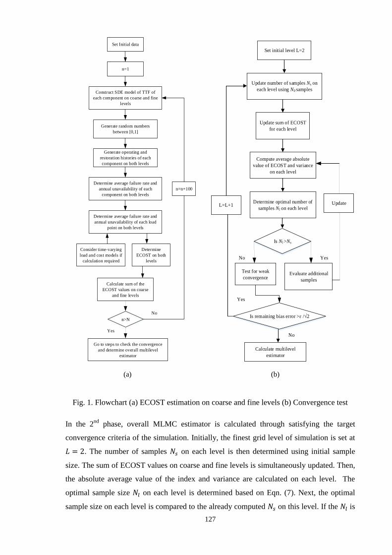
127

Set Initial data

n=1

Construct SDE model of TTF of

each component on coarse and fine

levels

Generate random numbers

between [0,1]

Generate operating and

restoration histories of each

component on both levels

Determine average failure rate and

annual unavailability of each

component on both levels

Determine average failure rate and

annual unavailability of each load

point on both levels

Consider time-varying

load and cost models if

calculation required

Determine

ECOST on both

levels

Calculate sum of the

ECOST values on coarse

and fine levels

Go to steps to check the convergence

and determine overall multilevel

estimator

n=n+100

n>N

No

Yes

Yes

No

Set initial level L=2

Update number of samples Ns on

each level using N0 samples

Update sum of ECOST

for each level

Determine optimal number of

samples Nl on each level

Calculate multilevel

estimator

UpdateL=L+1

Is Nl >Ns

Is remaining bias error >ɛ / 2

Compute average absolute

value of ECOST and variance

on each level

Test for weak

convergenceEvaluate additional

samples

YesNo

(a) (b)

Fig. 1. Flowchart (a) ECOST estimation on coarse and fine levels (b) Convergence test

In the 2nd

phase, overall MLMC estimator is calculated through satisfying the target

convergence criteria of the simulation. Initially, the finest grid level of simulation is set at

. The number of samples on each level is then determined using initial sample

size. The sum of ECOST values on coarse and fine levels is simultaneously updated. Then,

the absolute average value of the index and variance are calculated on each level. The

optimal sample size on each level is determined based on Eqn. (7). Next, the optimal

sample size on each level is compared to the already computed on this level. If the is

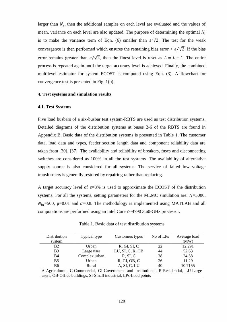
128

larger than , then the additional samples on each level are evaluated and the values of

mean, variance on each level are also updated. The purpose of determining the optimal

is to make the variance term of Eqn. (6) smaller than . The test for the weak

convergence is then performed which ensures the remaining bias error < . If the bias

error remains greater than , then the finest level is reset as . The entire

process is repeated again until the target accuracy level is achieved. Finally, the combined

multilevel estimator for system ECOST is computed using Eqn. (3). A flowchart for

convergence test is presented in Fig. 1(b).

4. Test systems and simulation results

4.1. Test Systems

Five load busbars of a six-busbar test system-RBTS are used as test distribution systems.

Detailed diagrams of the distribution systems at buses 2-6 of the RBTS are found in

Appendix B. Basic data of the distribution systems is presented in Table 1. The customer

data, load data and types, feeder section length data and component reliability data are

taken from [30], [37]. The availability and reliability of breakers, fuses and disconnecting

switches are considered as 100% in all the test systems. The availability of alternative

supply source is also considered for all systems. The service of failed low voltage

transformers is generally restored by repairing rather than replacing.

A target accuracy level of =3% is used to approximate the ECOST of the distribution

systems. For all the systems, setting parameters for the MLMC simulation are: =5000,

=500, =0.01 and =0.8. The methodology is implemented using MATLAB and all

computations are performed using an Intel Core i7-4790 3.60-GHz processor.

Table 1. Basic data of test distribution systems

Distribution

system

Typical type Customers types No of LPs Average load

(MW)

B2 Urban R, GI, SI, C 22 12.291

B3 Large user LU, SI, C, R, OB 44 52.63

B4 Complex urban R, SI, C 38 24.58

B5 Urban R, GI, OB, C 26 11.29

B6 Rural A, SI, C, LU 40 10.7155

A-Agricultural, C-Commercial, GI-Government and Institutional, R-Residential, LU-Large

users, OB-Office buildings, SI-Small industrial, LPs-Load points

129

4.2. Simulation results

4.2.1. Effect of network configuration and load type

Table 2 presents the effect of network configuration and load types in ECOST variation

using MC and MLMC methods based computation. The RBTS distribution systems

connected to five load buses (B2 to B6) are considered for this purpose [30]. By comparing

different test systems, it is seen that the maximum and minimum system ECOST values are

found in B3 and B6 systems, respectively. In Eqn. (17), we find that the amount of system

ECOST depends on the failure rate, load level and interruption cost of the interrupted load

points. In the B3 system, there are five types of loads such as residential, large users, small

industrial, commercial and office building users and the total amount of average load for

all 44 load points is 52.63 MW. On the other hand, in the B6 system, there are four types

of loads such as residential, small industrial, commercial and agricultural and the total

amount of average load for all 40 load points is 10.7155 MW. In most of the cases, average

load level per load point in the B3 system is higher than the B6 system. Due to having load

points with high interruption cost and duration in B3, it gives the large value of ECOST

than the B6 system.

More specifically, the availability of commercial load highly increases interruption cost for

all the systems except the B6 system, although the peak load level of this load type is not

maximum. This happens due to the large amount of per unit interruption cost for

commercial load type as displayed in SCDF [5]. In the B6 system, there are a large number

of residential load points, where only two commercial load points are connected to the

system.

The magnitude of ECOST also varies with the network topologies and loading types.

Interruptions in different load connected systems have very different consequences. A test

system with smaller number of load points, but having supplies to commercial customers

(due to huge interruption cost) may increase the ECOST value in the peak period.

For validation, the results obtained from the proposed method should agree with the results

from the analytical method. E[MC] and E[MLMC] are the percentages of the difference of

ECOST values using MC and MLMC methods with respect to the analytical value. The

results show that the ECOST values using MLMC method are very close to the values

from MC and analytical methods. The absolute value of maximum E[MLMC] is 3.25% for

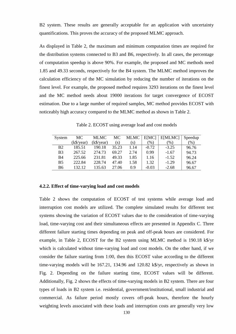
130

B2 system. These results are generally acceptable for an application with uncertainty

quantifications. This proves the accuracy of the proposed MLMC approach.

As displayed in Table 2, the maximum and minimum computation times are required for

the distribution systems connected to B3 and B6, respectively. In all cases, the percentage

of computation speedup is above 90%. For example, the proposed and MC methods need

1.85 and 49.33 seconds, respectively for the B4 system. The MLMC method improves the

calculation efficiency of the MC simulation by reducing the number of iterations on the

finest level. For example, the proposed method requires 3293 iterations on the finest level

and the MC method needs about 19000 iterations for target convergence of ECOST

estimation. Due to a large number of required samples, MC method provides ECOST with

noticeably high accuracy compared to the MLMC method as shown in Table 2.

Table 2. ECOST using average load and cost models

System MC (k$/year)

MLMC (k$/year)

MC (s)

MLMC (s)

E[MC] (%)

E[MLMC] (%)

Speedup (%)

B2 185.51 190.18 35.23 1.14 -0.72 -3.25 96.76 B3 267.52 274.73 69.27 2.74 0.99 -1.67 94.73 B4 225.66 231.81 49.33 1.85 1.16 -1.52 96.24 B5 222.84 228.74 47.40 1.58 1.32 -1.29 96.67 B6 132.12 135.63 27.06 0.9 -0.03 -2.68 96.67

4.2.2. Effect of time-varying load and cost models

Table 2 shows the computation of ECOST of test systems while average load and

interruption cost models are utilized. The complete simulated results for different test

systems showing the variation of ECOST values due to the consideration of time-varying

load, time-varying cost and their simultaneous effects are presented in Appendix C. Three

different failure starting times depending on peak and off-peak hours are considered. For

example, in Table 2, ECOST for the B2 system using MLMC method is 190.18 k$/yr

which is calculated without time-varying load and cost models. On the other hand, if we

consider the failure starting from 1:00, then this ECOST value according to the different

time-varying models will be 167.21, 134.96 and 120.82 k$/yr, respectively as shown in

Fig. 2. Depending on the failure starting time, ECOST values will be different.

Additionally, Fig. 2 shows the effects of time-varying models in B2 system. There are four

types of loads in B2 system i.e. residential, government/institutional, small industrial and

commercial. As failure period mostly covers off-peak hours, therefore the hourly

weighting levels associated with these loads and interruption costs are generally very low

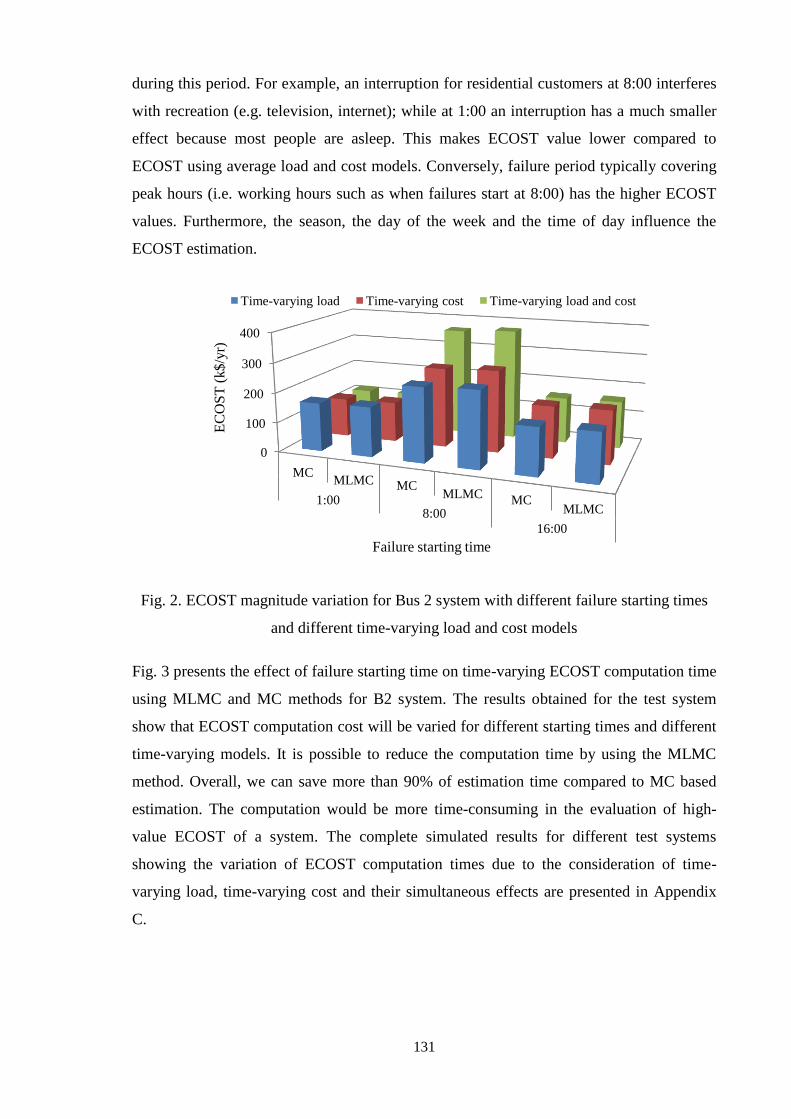
131

during this period. For example, an interruption for residential customers at 8:00 interferes

with recreation (e.g. television, internet); while at 1:00 an interruption has a much smaller

effect because most people are asleep. This makes ECOST value lower compared to

ECOST using average load and cost models. Conversely, failure period typically covering

peak hours (i.e. working hours such as when failures start at 8:00) has the higher ECOST

values. Furthermore, the season, the day of the week and the time of day influence the

ECOST estimation.

Fig. 2. ECOST magnitude variation for Bus 2 system with different failure starting times

and different time-varying load and cost models

Fig. 3 presents the effect of failure starting time on time-varying ECOST computation time

using MLMC and MC methods for B2 system. The results obtained for the test system

show that ECOST computation cost will be varied for different starting times and different

time-varying models. It is possible to reduce the computation time by using the MLMC

method. Overall, we can save more than 90% of estimation time compared to MC based

estimation. The computation would be more time-consuming in the evaluation of high-

value ECOST of a system. The complete simulated results for different test systems

showing the variation of ECOST computation times due to the consideration of time-

varying load, time-varying cost and their simultaneous effects are presented in Appendix

C.

0

100

200

300

400

MC MLMC MC

MLMC MC

MLMC 1:00

8:00

16:00

EC

OS

T (

k$

/yr)

Failure starting time

Time-varying load Time-varying cost Time-varying load and cost

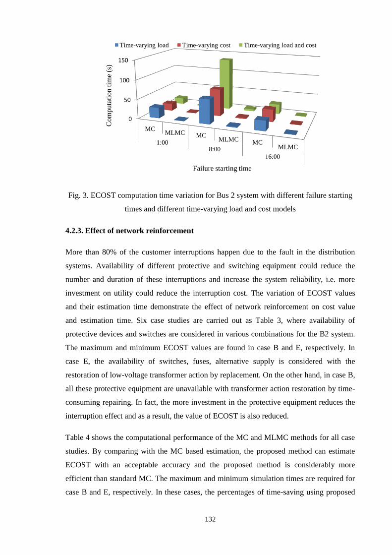
132

Fig. 3. ECOST computation time variation for Bus 2 system with different failure starting

times and different time-varying load and cost models

4.2.3. Effect of network reinforcement

More than 80% of the customer interruptions happen due to the fault in the distribution

systems. Availability of different protective and switching equipment could reduce the

number and duration of these interruptions and increase the system reliability, i.e. more

investment on utility could reduce the interruption cost. The variation of ECOST values

and their estimation time demonstrate the effect of network reinforcement on cost value

and estimation time. Six case studies are carried out as Table 3, where availability of

protective devices and switches are considered in various combinations for the B2 system.

The maximum and minimum ECOST values are found in case B and E, respectively. In

case E, the availability of switches, fuses, alternative supply is considered with the

restoration of low-voltage transformer action by replacement. On the other hand, in case B,

all these protective equipment are unavailable with transformer action restoration by time-

consuming repairing. In fact, the more investment in the protective equipment reduces the

interruption effect and as a result, the value of ECOST is also reduced.

Table 4 shows the computational performance of the MC and MLMC methods for all case

studies. By comparing with the MC based estimation, the proposed method can estimate

ECOST with an acceptable accuracy and the proposed method is considerably more

efficient than standard MC. The maximum and minimum simulation times are required for

case B and E, respectively. In these cases, the percentages of time-saving using proposed

0

50

100

150

MC MLMC MC

MLMC MC

MLMC 1:00

8:00

16:00

Co

mp

uta

tio

n t

ime

(s)

Failure starting time

Time-varying load Time-varying cost Time-varying load and cost

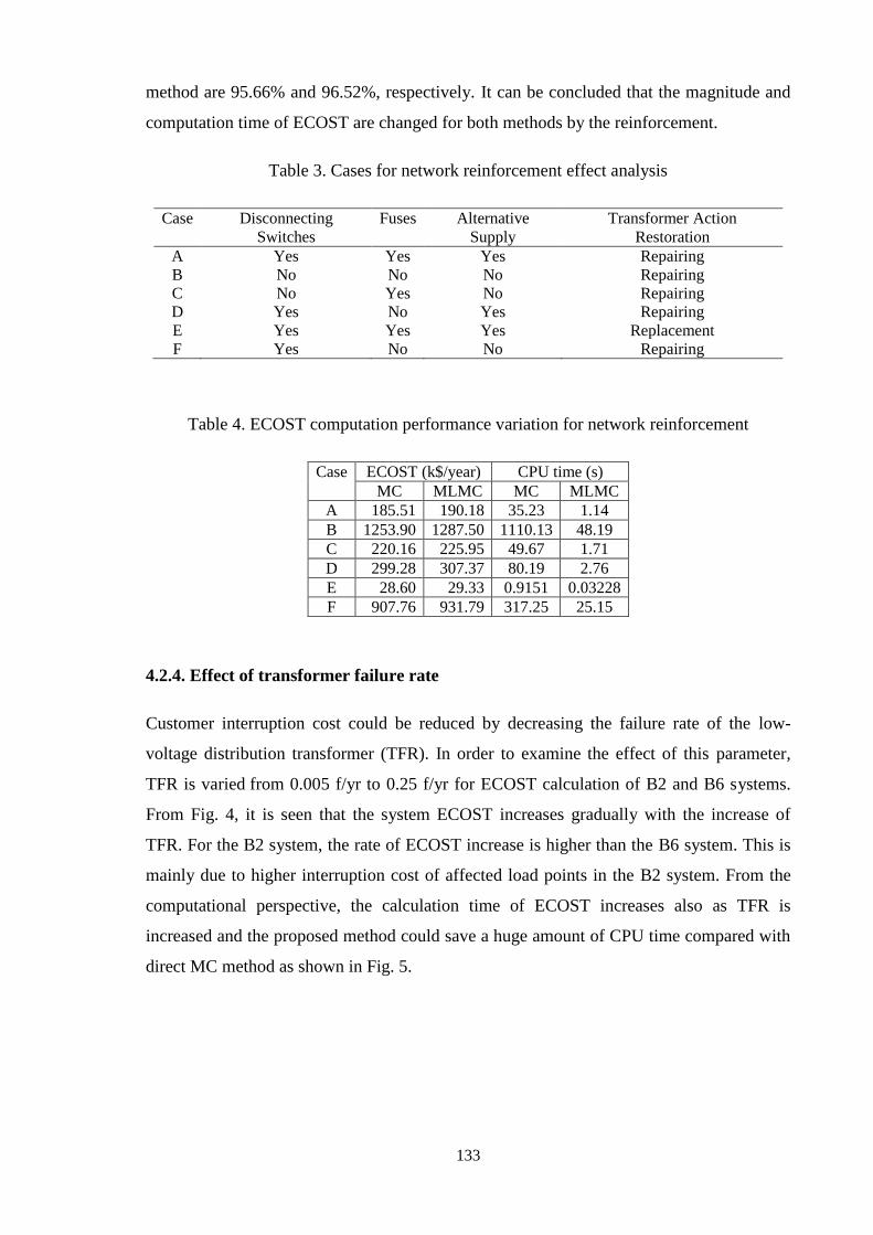
133

method are 95.66% and 96.52%, respectively. It can be concluded that the magnitude and

computation time of ECOST are changed for both methods by the reinforcement.

Table 3. Cases for network reinforcement effect analysis

Case Disconnecting

Switches

Fuses Alternative

Supply

Transformer Action

Restoration

A Yes Yes Yes Repairing

B No No No Repairing

C No Yes No Repairing

D Yes No Yes Repairing

E Yes Yes Yes Replacement

F Yes No No Repairing

Table 4. ECOST computation performance variation for network reinforcement

Case ECOST (k$/year) CPU time (s)

MC MLMC MC MLMC

A 185.51 190.18 35.23 1.14

B 1253.90 1287.50 1110.13 48.19

C 220.16 225.95 49.67 1.71

D 299.28 307.37 80.19 2.76

E 28.60 29.33 0.9151 0.03228

F 907.76 931.79 317.25 25.15

4.2.4. Effect of transformer failure rate

Customer interruption cost could be reduced by decreasing the failure rate of the low-

voltage distribution transformer (TFR). In order to examine the effect of this parameter,

TFR is varied from 0.005 f/yr to 0.25 f/yr for ECOST calculation of B2 and B6 systems.

From Fig. 4, it is seen that the system ECOST increases gradually with the increase of

TFR. For the B2 system, the rate of ECOST increase is higher than the B6 system. This is

mainly due to higher interruption cost of affected load points in the B2 system. From the

computational perspective, the calculation time of ECOST increases also as TFR is

increased and the proposed method could save a huge amount of CPU time compared with

direct MC method as shown in Fig. 5.

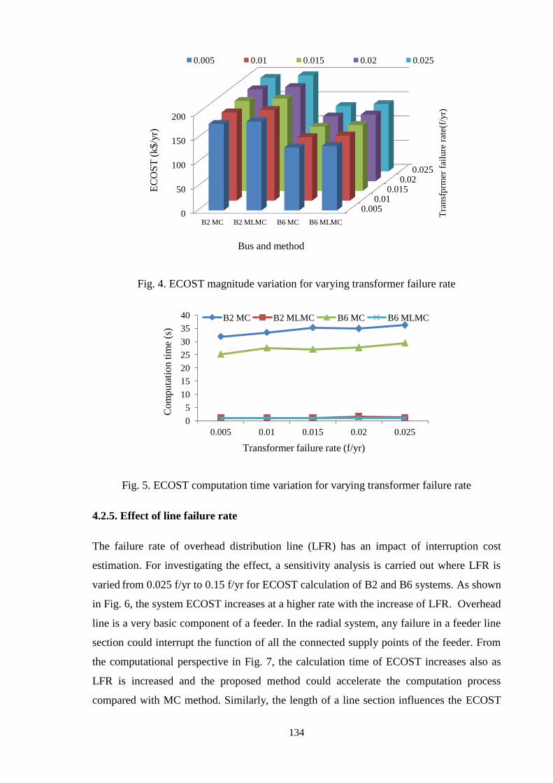
134

Fig. 4. ECOST magnitude variation for varying transformer failure rate

Fig. 5. ECOST computation time variation for varying transformer failure rate

4.2.5. Effect of line failure rate

The failure rate of overhead distribution line (LFR) has an impact of interruption cost

estimation. For investigating the effect, a sensitivity analysis is carried out where LFR is

varied from 0.025 f/yr to 0.15 f/yr for ECOST calculation of B2 and B6 systems. As shown

in Fig. 6, the system ECOST increases at a higher rate with the increase of LFR. Overhead

line is a very basic component of a feeder. In the radial system, any failure in a feeder line

section could interrupt the function of all the connected supply points of the feeder. From

the computational perspective in Fig. 7, the calculation time of ECOST increases also as

LFR is increased and the proposed method could accelerate the computation process

compared with MC method. Similarly, the length of a line section influences the ECOST

0.005 0.01

0.015 0.02

0.025

0

50

100

150

200

B2 MC B2 MLMC B6 MC B6 MLMC

Tra

nsf

prm

er f

ailu

re r

ate(

f/yr)

EC

OS

T (

k$

/yr)

Bus and method

0.005 0.01 0.015 0.02 0.025

0

5

10

15

20

25

30

35

40

0.005 0.01 0.015 0.02 0.025

Com

puta

tion t

ime

(s)

Transformer failure rate (f/yr)


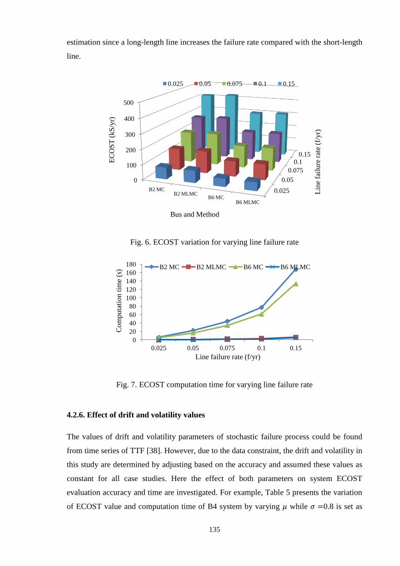
135

estimation since a long-length line increases the failure rate compared with the short-length

line.

Fig. 6. ECOST variation for varying line failure rate

Fig. 7. ECOST computation time for varying line failure rate

4.2.6. Effect of drift and volatility values

The values of drift and volatility parameters of stochastic failure process could be found

from time series of TTF [38]. However, due to the data constraint, the drift and volatility in

this study are determined by adjusting based on the accuracy and assumed these values as

constant for all case studies. Here the effect of both parameters on system ECOST

evaluation accuracy and time are investigated. For example, Table 5 presents the variation

of ECOST value and computation time of B4 system by varying while 0.8 is set as

0.025

0.05

0.075

0.1 0.15

0

100

200

300

400

500

B2 MC B2 MLMC

B6 MC B6 MLMC

Lin

e fa

ilu

re r

ate

(f/y

r)

EC

OS

T (

kS

/yr)

Bus and Method

0.025 0.05 0.075 0.1 0.15

0

20

40

60

80

100

120

140

160

180

0.025 0.05 0.075 0.1 0.15

Com

puta

tion t

ime

(s)

Line failure rate (f/yr)


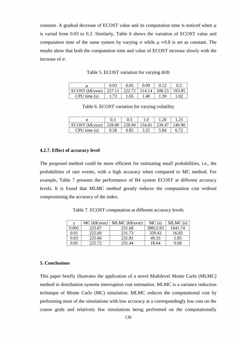
136

constant. A gradual decrease of ECOST value and its computation time is noticed when

is varied from 0.03 to 0.2. Similarly, Table 6 shows the variation of ECOST value and

computation time of the same system by varying while 0.8 is set as constant. The

results show that both the computation time and value of ECOST increase slowly with the

increase of .

Table 5. ECOST variation for varying drift

0.03 0.05 0.09 0.12 0.2

ECOST (k$/year) 227.11 222.72 214.14 208.23 193.85

CPU time (s) 1.73 1.65 1.40 1.30 1.02

Table 6. ECOST variation for varying volatility

0.3 0.5 1.0 1.20 1.25

ECOST (k$/year) 228.80 228.90 234.81 239.47 240.90

CPU time (s) 0.58 0.85 3.25 5.84 6.72

4.2.7. Effect of accuracy level

The proposed method could be more efficient for estimating small probabilities, i.e., the

probabilities of rare events, with a high accuracy when compared to MC method. For

example, Table 7 presents the performance of B4 system ECOST at different accuracy

levels. It is found that MLMC method greatly reduces the computation cost without

compromising the accuracy of the index.

Table 7. ECOST computation at different accuracy levels

MC (k$/year) MLMC (k$/year) MC (s) MLMC (s)

0.001 225.67 231.68 38812.93 1641.74 0.01 225.69 231.73 359.43 16.83 0.03 225.66 231.81 49.33 1.85 0.05 225.72 231.44 18.64 0.68

5. Conclusions

This paper briefly illustrates the application of a novel Multilevel Monte Carlo (MLMC)

method in distribution systems interruption cost estimation. MLMC is a variance reduction

technique of Monte Carlo (MC) simulation. MLMC reduces the computational cost by

performing most of the simulations with low accuracy at a correspondingly low cost on the

coarse grids and relatively few simulations being performed on the computationally

137

expensive fine grids at high accuracy and high cost. Both accuracy and computational

efficiency of the MLMC are considered to demonstrate the practicability of the proposed

method. Comparisons of results obtained using the basic MC simulation are presented. The

results show that the proposed method could estimate the average customer interruption

cost accurately and also gives a significant speed-up over the MC based computation.

A number of sensitivity analyses have been carried out to show the effect of different

parameters on the computation process. We found that network configuration and load


failure rate, drift and volatility values parameters have a considerable effect of MLMC

based system ECOST computation.

Due to the data constraint, the research on comparisons with other advanced MC methods

and the probability distributions of MLMC [39] based ECOST estimations will be carried

out in the future. For estimating MLMC Maximum Entropy method based PDF in the

current study, the authors believe that more studies should be conducted where some

additional algorithms, coding, methodology, sensitivity studies of some assumptions (such

as number of moments in the Maximum Entropy method) need to be completed for

ECOST analysis in order to publish the PDF. Therefore, in the present publication, we set

our main focus to provide the MLMC based ECOST estimation to show its speed-up

capability and also to present some sensitivity analysis which is necessary to analyse the

large real-life systems. The computationally efficient algorithm and simulation examples

presented in this paper would potentially help system planners to collect the useful

information of reliability cost of their respective distribution systems. We believe that the

proposed algorithm will be able to speed up the decision-making process in reliability

improvement process.

References

[1] R. Billinton, S. Ali, G. Wacker, Rural distribution system reliability worth

evaluation using individual customer outage cost characteristics, Int J Electr Power

Energy Syst 26 (2004) 235-240.

[2] M. De Nooij, C. Koopmans, C. Bijvoet, The value of supply security: the costs of

power interruptions: Economic input for damage reduction and investment in

networks, Energy Econ 29 (2007) 277-295.

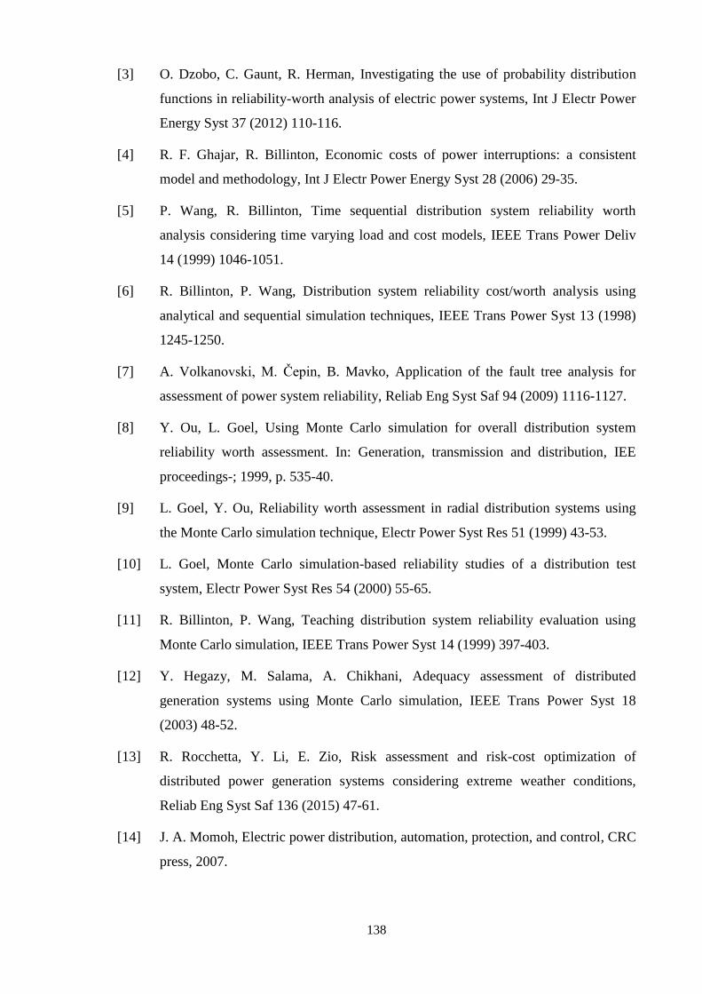
138

[3] O. Dzobo, C. Gaunt, R. Herman, Investigating the use of probability distribution

functions in reliability-worth analysis of electric power systems, Int J Electr Power

Energy Syst 37 (2012) 110-116.

[4] R. F. Ghajar, R. Billinton, Economic costs of power interruptions: a consistent

model and methodology, Int J Electr Power Energy Syst 28 (2006) 29-35.

[5] P. Wang, R. Billinton, Time sequential distribution system reliability worth

analysis considering time varying load and cost models, IEEE Trans Power Deliv

14 (1999) 1046-1051.

[6] R. Billinton, P. Wang, Distribution system reliability cost/worth analysis using

analytical and sequential simulation techniques, IEEE Trans Power Syst 13 (1998)

1245-1250.

[7] A. Volkanovski, M. Čepin, B. Mavko, Application of the fault tree analysis for

assessment of power system reliability, Reliab Eng Syst Saf 94 (2009) 1116-1127.

[8] Y. Ou, L. Goel, Using Monte Carlo simulation for overall distribution system

reliability worth assessment. In: Generation, transmission and distribution, IEE

proceedings-; 1999, p. 535-40.

[9] L. Goel, Y. Ou, Reliability worth assessment in radial distribution systems using

the Monte Carlo simulation technique, Electr Power Syst Res 51 (1999) 43-53.

[10] L. Goel, Monte Carlo simulation-based reliability studies of a distribution test

system, Electr Power Syst Res 54 (2000) 55-65.

[11] R. Billinton, P. Wang, Teaching distribution system reliability evaluation using

Monte Carlo simulation, IEEE Trans Power Syst 14 (1999) 397-403.

[12] Y. Hegazy, M. Salama, A. Chikhani, Adequacy assessment of distributed

generation systems using Monte Carlo simulation, IEEE Trans Power Syst 18

(2003) 48-52.

[13] R. Rocchetta, Y. Li, E. Zio, Risk assessment and risk-cost optimization of

distributed power generation systems considering extreme weather conditions,

Reliab Eng Syst Saf 136 (2015) 47-61.

[14] J. A. Momoh, Electric power distribution, automation, protection, and control, CRC

press, 2007.

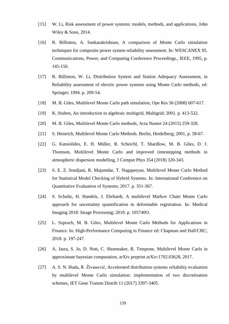
139

[15] W. Li, Risk assessment of power systems: models, methods, and applications, John

Wiley & Sons, 2014.

[16] R. Billinton, A. Sankarakrishnan, A comparison of Monte Carlo simulation

techniques for composite power system reliability assessment. In: WESCANEX 95.

Communications, Power, and Computing Conference Proceedings., IEEE, 1995, p.

145-150.

[17] R. Billinton, W. Li, Distribution System and Station Adequacy Assessment, in

Reliability assessment of electric power systems using Monte Carlo methods, ed:

Springer; 1994. p. 209-54.

[18] M. B. Giles, Multilevel Monte Carlo path simulation, Ope Res 56 (2008) 607-617.

[19] K. Stuben, An introduction to algebraic multigrid, Multigrid; 2001. p. 413-532.

[20] M. B. Giles, Multilevel Monte Carlo methods, Acta Numer 24 (2015) 259-328.

[21] S. Heinrich, Multilevel Monte Carlo Methods. Berlin, Heidelberg; 2001, p. 58-67.

[22] G. Katsiolides, E. H. Müller, R. Scheichl, T. Shardlow, M. B. Giles, D. J.

Thomson, Multilevel Monte Carlo and improved timestepping methods in

atmospheric dispersion modelling, J Comput Phys 354 (2018) 320-343.

[23] S. E. Z. Soudjani, R. Majumdar, T. Nagapetyan, Multilevel Monte Carlo Method

for Statistical Model Checking of Hybrid Systems. In: International Conference on

Quantitative Evaluation of Systems; 2017. p. 351-367.

[24] S. Schultz, H. Handels, J. Ehrhardt, A multilevel Markov Chain Monte Carlo

approach for uncertainty quantification in deformable registration. In: Medical

Imaging 2018: Image Processing; 2018. p. 105740O.

[25] L. Szpruch, M. B. Giles, Multilevel Monte Carlo Methods for Applications in

Finance. In: High-Performance Computing in Finance ed: Chapman and Hall/CRC;

2018. p. 197-247.

[26] A. Jasra, S. Jo, D. Nott, C. Shoemaker, R. Tempone, Multilevel Monte Carlo in

approximate bayesian computation, arXiv preprint arXiv:1702.03628, 2017.

[27] A. S. N. Huda, R. Živanović, Accelerated distribution systems reliability evaluation

by multilevel Monte Carlo simulation: implementation of two discretisation

schemes, IET Gene Transm Distrib 11 (2017) 3397-3405.

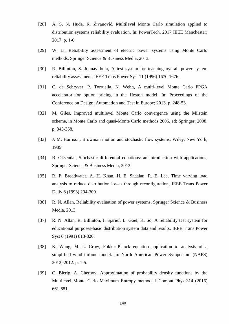
140

[28] A. S. N. Huda, R. Živanović. Multilevel Monte Carlo simulation applied to

distribution systems reliability evaluation. In: PowerTech, 2017 IEEE Manchester;

2017. p. 1-6.

[29] W. Li, Reliability assessment of electric power systems using Monte Carlo

methods, Springer Science & Business Media, 2013.

[30] R. Billinton, S. Jonnavithula, A test system for teaching overall power system

reliability assessment, IEEE Trans Power Syst 11 (1996) 1670-1676.

[31] C. de Schryver, P. Torruella, N. Wehn, A multi-level Monte Carlo FPGA

accelerator for option pricing in the Heston model. In: Proceedings of the

Conference on Design, Automation and Test in Europe; 2013. p. 248-53.

[32] M. Giles, Improved multilevel Monte Carlo convergence using the Milstein

scheme, in Monte Carlo and quasi-Monte Carlo methods 2006, ed: Springer; 2008.

p. 343-358.

[33] J. M. Harrison, Brownian motion and stochastic flow systems, Wiley, New York,

1985.

[34] B. Oksendal, Stochastic differential equations: an introduction with applications,

Springer Science & Business Media, 2013.

[35] R. P. Broadwater, A. H. Khan, H. E. Shaalan, R. E. Lee, Time varying load

analysis to reduce distribution losses through reconfiguration, IEEE Trans Power

Deliv 8 (1993) 294-300.

[36] R. N. Allan, Reliability evaluation of power systems, Springer Science & Business

Media, 2013.

[37] R. N. Allan, R. Billinton, I. Sjarief, L. Goel, K. So, A reliability test system for

educational purposes-basic distribution system data and results, IEEE Trans Power

Syst 6 (1991) 813-820.

[38] K. Wang, M. L. Crow, Fokker-Planck equation application to analysis of a

simplified wind turbine model. In: North American Power Symposium (NAPS)

2012; 2012. p. 1-5.

[39] C. Bierig, A. Chernov, Approximation of probability density functions by the

Multilevel Monte Carlo Maximum Entropy method, J Comput Phys 314 (2016)

661-681.

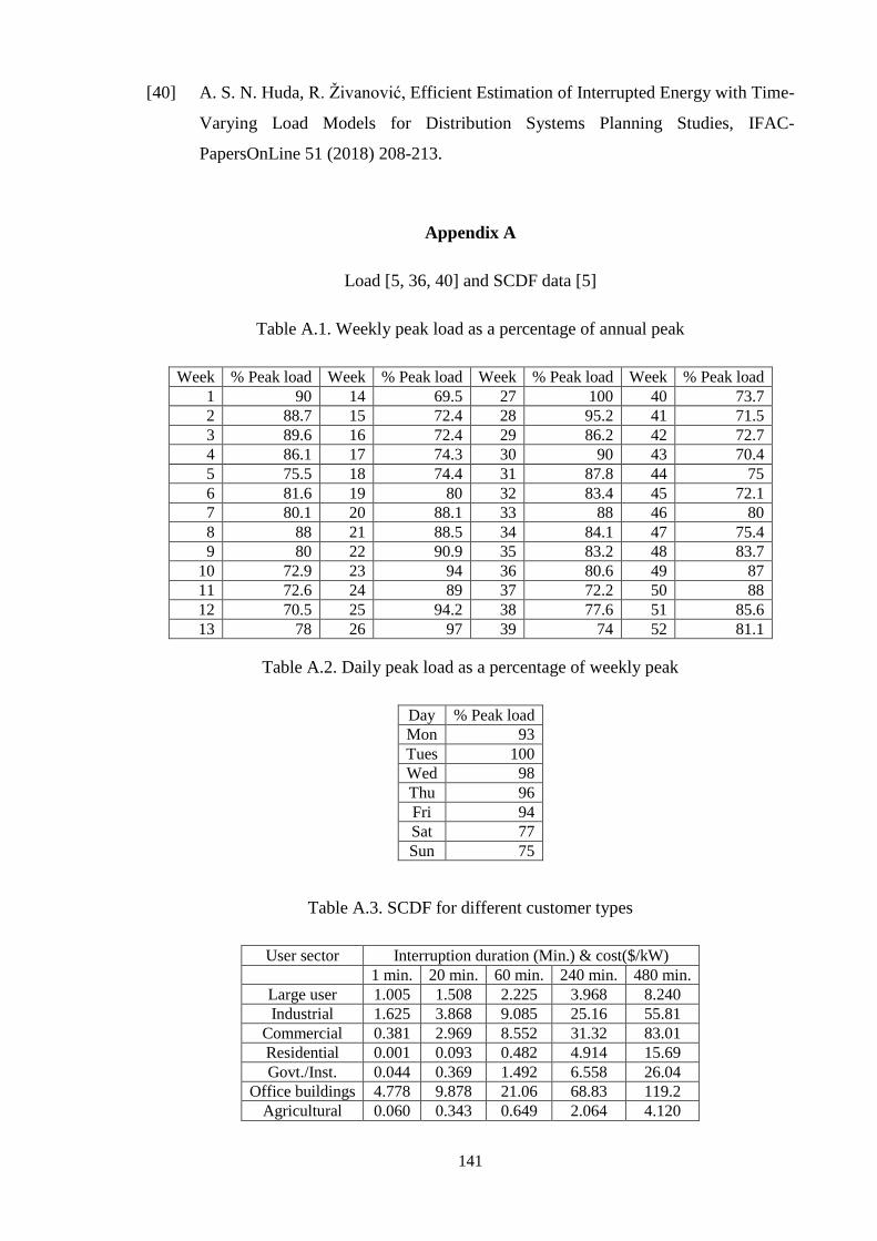
141

[40] A. S. N. Huda, R. Živanović, Efficient Estimation of Interrupted Energy with Time-

Varying Load Models for Distribution Systems Planning Studies, IFAC-

PapersOnLine 51 (2018) 208-213.

Appendix A

Load [5, 36, 40] and SCDF data [5]

Table A.1. Weekly peak load as a percentage of annual peak

Week % Peak load Week % Peak load Week % Peak load Week % Peak load

1 90 14 69.5 27 100 40 73.7

2 88.7 15 72.4 28 95.2 41 71.5

3 89.6 16 72.4 29 86.2 42 72.7

4 86.1 17 74.3 30 90 43 70.4

5 75.5 18 74.4 31 87.8 44 75

6 81.6 19 80 32 83.4 45 72.1

7 80.1 20 88.1 33 88 46 80

8 88 21 88.5 34 84.1 47 75.4

9 80 22 90.9 35 83.2 48 83.7

10 72.9 23 94 36 80.6 49 87

11 72.6 24 89 37 72.2 50 88

12 70.5 25 94.2 38 77.6 51 85.6

13 78 26 97 39 74 52 81.1

Table A.2. Daily peak load as a percentage of weekly peak

Day % Peak load

Mon 93

Tues 100

Wed 98

Thu 96

Fri 94

Sat 77

Sun 75

Table A.3. SCDF for different customer types

User sector Interruption duration (Min.) & cost($/kW)

1 min. 20 min. 60 min. 240 min. 480 min.

Large user 1.005 1.508 2.225 3.968 8.240

Industrial 1.625 3.868 9.085 25.16 55.81

Commercial 0.381 2.969 8.552 31.32 83.01

Residential 0.001 0.093 0.482 4.914 15.69

Govt./Inst. 0.044 0.369 1.492 6.558 26.04

Office buildings 4.778 9.878 21.06 68.83 119.2

Agricultural 0.060 0.343 0.649 2.064 4.120

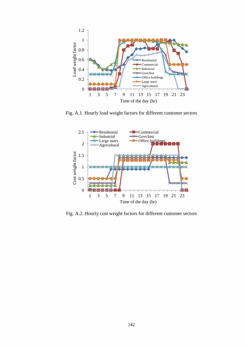
142

Fig. A.1. Hourly load weight factors for different customer sectors

Fig. A.2. Hourly cost weight factors for different customer sectors

0

0.2

0.4

0.6

0.8

1

1.2

1 3 5 7 9 11 13 15 17 19 21 23

Lo

ad w

eigh

t fa

cto

r

Time of the day (hr)

Residential

Commercial

Industrial

Govt/Inst

Office buildings

Large users

Agricultural

0

0.5

1

1.5

2

2.5

1 3 5 7 9 11 13 15 17 19 21 23

Cost

wei

ght

fact

or

Time of the day (hr)

Residential Commercial Industrial Govt/Inst Large users Office buildings Agricultural

143

Appendix B

Single line diagrams of distribution systems [30]

LP17

1110

18

12

Substation

33/11 kV

F1

3

45 6

78 9


F2

LP9 LP8

12

13

14

15


16

1719

20

21

22 23

24

25

F4

LP18 LP19 LP20 LP21 LP22

26

27 28

29

3031

32

3335

34

36

F3

N/O

N/O

LP16

(a)

11 kV

N/O

F1

N/O

F2 13

LP7

LP31 LP30 LP29

LP34 LP33

11 kV

11 kV

138 kV

F3

F4

F5

F6

F7F8

LP2 LP1LP3LP4LP5LP6

LP8LP9LP10

LP11LP12LP13LP14LP15LP16LP17

LP18LP19LP20LP22LP24

LP26LP28

LP23LP21

LP25LP27

LP41

LP43

LP32

LP44 LP42

LP35LP36LP37LP38

LP39LP40

12

4 1

18

17

16 14

15

19

2024

313236

4344

45

4647

48

49

5051

5253

54

5556

5758

59

6061

6364

6265

6667

7273

74

7576

77

6869

70

71

(b)

138 KV

11 KV

LP22 LP23 LP20

34

LP21 LP24 LP25 LP26

F4

33

35

36

37 38

39

4042

41

43

N/O

1110

25

12

F1

3

45 6

78 9


F212

13

14

LP14 LP15 LP16

23

2426

27

28 30 F3

N/O


15

16

17

18

19 21

20

22

LP18 LP19

31 32

LP17

29

(d)

N/O

45

46

47

48

33 kV33 kV33 kV

11 kV11 kV

11 kV

F3F2F1F7F6F5F4

1913150

4431

20

21

22

23

24

25

26

27

28

29

30

14

15

16

17

18

2

3

4

5

6

7

8

9

10

11

12

57

58

59

60

61

62

63

64

65

66

67

51

52

53

54

55

49

32

33

34

35

36

37

38

39

40

41

42

43

LP11

LP12

LP13

LP14

LP15

LP16

LP17

LP8

LP9

LP10

56

LP1

LP2

LP3

LP4

LP5

LP6

LP7

LP32

LP33

LP34

LP35

LP36

LP37

LP38

LP29

LP30

LP31

LP26

LP27

LP28

LP18

LP19

LP20

LP21

LP22

LP23

LP24

LP25

N/O

N/O

N/O

SP1SP2SP3

(c)

22 LP11

2 LP1

4 LP2

6 LP3

8 LP4

10 LP5

12 LP6

LP18 36

LP20 38

LP22 40

LP24

LP31

LP32

LP33

LP34

LP35

LP28

LP29

LP30

37 LP19

LP21

LP23

LP25

47

LP26

LP27

LP36

LP14 28

LP17 34

30

32

27

29

31

33

1

3

5

7

9

11

13

15

17

19

21

23

25

35

39

LP37 LP38 LP39 LP40

42

41

43

44

53

54

55

56

57

58

50

51

52

59

60

6162 63 64

49

48

46

45

F2F1F3

F4

LP15

LP16

14 LP7

16 LP8

18 LP9

20 LP10

24 LP12

26 LP13

N/O

33KV

(e)

Fig. B.1. Distribution systems for RBTS (a) Bus 2 (b) Bus 3 (c) Bus 4 (d) Bus 5 and (e)

Bus 6

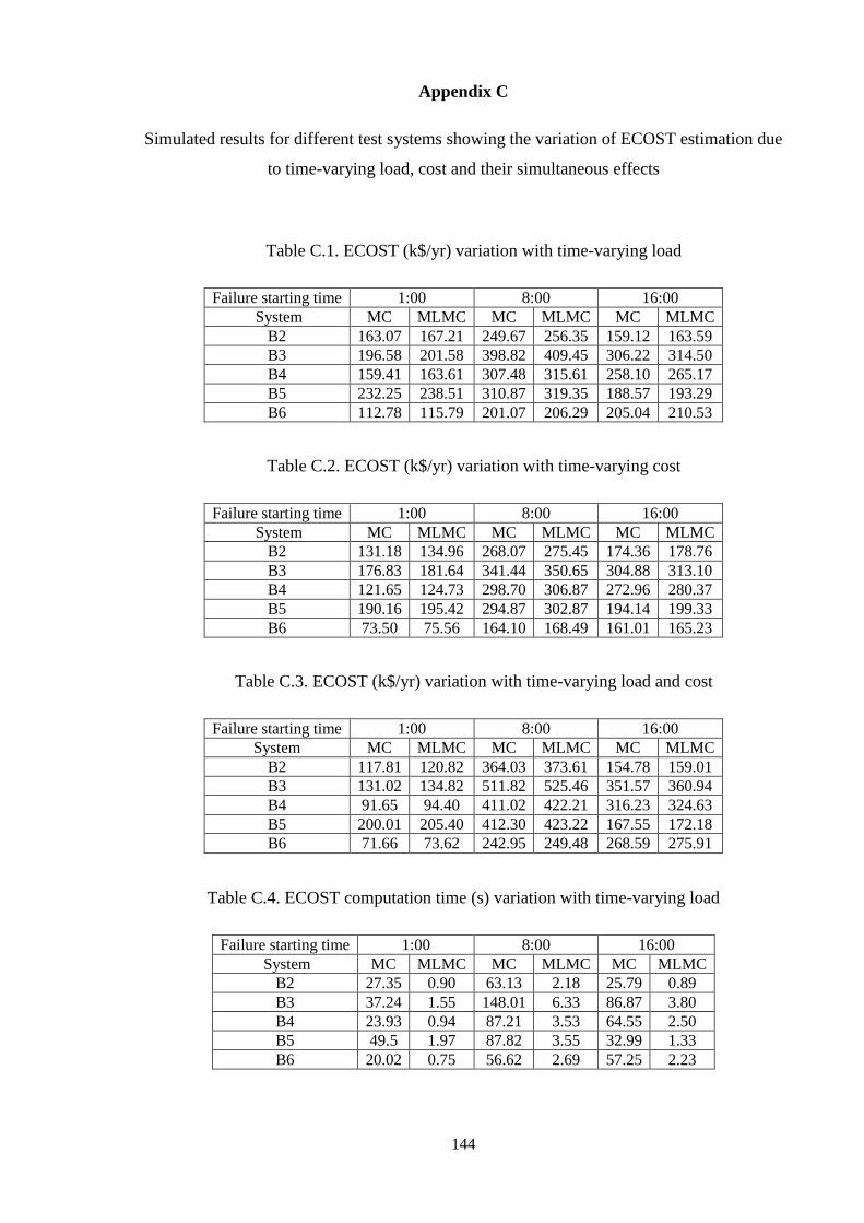
144

Appendix C

Simulated results for different test systems showing the variation of ECOST estimation due

to time-varying load, cost and their simultaneous effects

Table C.1. ECOST (k$/yr) variation with time-varying load

Failure starting time 1:00 8:00 16:00

System MC MLMC MC MLMC MC MLMC

B2 163.07 167.21 249.67 256.35 159.12 163.59

B3 196.58 201.58 398.82 409.45 306.22 314.50

B4 159.41 163.61 307.48 315.61 258.10 265.17

B5 232.25 238.51 310.87 319.35 188.57 193.29

B6 112.78 115.79 201.07 206.29 205.04 210.53

Table C.2. ECOST (k$/yr) variation with time-varying cost



B2 131.18 134.96 268.07 275.45 174.36 178.76

B3 176.83 181.64 341.44 350.65 304.88 313.10

B4 121.65 124.73 298.70 306.87 272.96 280.37

B5 190.16 195.42 294.87 302.87 194.14 199.33

B6 73.50 75.56 164.10 168.49 161.01 165.23

Table C.3. ECOST (k$/yr) variation with time-varying load and cost



B2 117.81 120.82 364.03 373.61 154.78 159.01

B3 131.02 134.82 511.82 525.46 351.57 360.94

B4 91.65 94.40 411.02 422.21 316.23 324.63

B5 200.01 205.40 412.30 423.22 167.55 172.18

B6 71.66 73.62 242.95 249.48 268.59 275.91

Table C.4. ECOST computation time (s) variation with time-varying load



B2 27.35 0.90 63.13 2.18 25.79 0.89

B3 37.24 1.55 148.01 6.33 86.87 3.80

B4 23.93 0.94 87.21 3.53 64.55 2.50

B5 49.5 1.97 87.82 3.55 32.99 1.33

B6 20.02 0.75 56.62 2.69 57.25 2.23

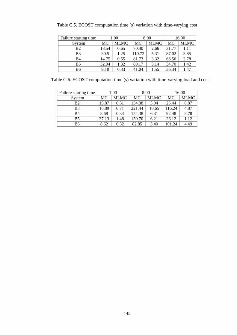
145

Table C.5. ECOST computation time (s) variation with time-varying cost



B2 18.54 0.65 70.40 2.66 31.77 1.11

B3 30.5 1.25 110.72 5.31 87.02 3.85

B4 14.75 0.55 81.73 3.32 66.56 2.78

B5 32.94 1.32 80.17 3.14 34.70 1.42

B6 9.10 0.33 41.04 1.55 36.34 1.47

Table C.6. ECOST computation time (s) variation with time-varying load and cost



B2 15.87 0.51 134.38 5.04 25.44 0.87

B3 16.89 0.71 221.44 10.65 116.24 4.87

B4 8.68 0.34 154.38 6.31 92.48 3.78

B5 37.13 1.48 150.70 6.21 26.12 1.12

B6 8.62 0.32 82.85 3.40 101.24 4.49

146

Chapter 7

Effect of Weather Conditions on Computation

147


Title of Paper Analysis effect of weather conditions on electric distribution system reliability evaluation

through an efficient approach





manuscript style

Publication Details A. S. Nazmul Huda, Rastko Živanović (2018) Analysis effect of weather conditions on electric

distribution system reliability evaluation through an efficient approach, Quality and Reliability

Engineering International. Wiley.

Received feedback from reviewers

Principal author


(Candidate)

A. S. Nazmul Huda



manuscript.





paper.










148

Analysis effect of weather conditions on electric distribution system reliability

evaluation through an efficient approach

Abstract- The objective of this paper is to evaluate the distribution system reliability

indices under normal and adverse weather conditions while a new computationally

efficient Multilevel Monte Carlo (MLMC) simulation approach is used as a computation

tool. The evaluation of distribution system reliability in different weather conditions such

as high winds, lightning can be characterized by incorporating time-varying failure rate

and repair time of the failed components since these can be changed dramatically in

adverse weather condition. Application of classic MC simulation is usually sufficient to

evaluate the reliability accurately. However the increase of the computation speed of the

time-consuming MC method based evaluation especially while dealing with the rare events

could be an important contribution in modern power systems computation applications.

MLMC method is a recently developed variance reduction technique for MC method

which could reduce computation burden dramatically while both sampling and

discretization errors are considered for converging to a controllable accuracy level. For

validation purpose, applications of the implemented method are carried out on a

benchmark test distribution system. The effects of the reliability estimation considering

both normal and adverse weather effects on the computation performance are determined.

The results are compared with those obtained by using typical MC simulation.

Keywords- Distribution system reliability; Simulation speedup; Multilevel Monte Carlo

method; Weather effects.

1. Introduction

Reliability evaluation is an important prerequisite for designing and planning of power

distribution systems. It reveals the ability of a system to meet the load requirement of

customers in an economical way with minimal interruption [1]. About 20% of the load

point interruptions happen due to the failures in generation and transmission systems and

remaining 80% are caused by the problems in distribution systems [2]. The evaluation

measures some indices of interruption frequency and duration based on network

configuration and connected elements failure and repair information which supports a

distribution system planner to access most of the required knowledge about expected

frequency, duration, cost and energy loss of interruptions. The common indices concerning

these are System Average Interruption Frequency Index (SAIFI) and System Average

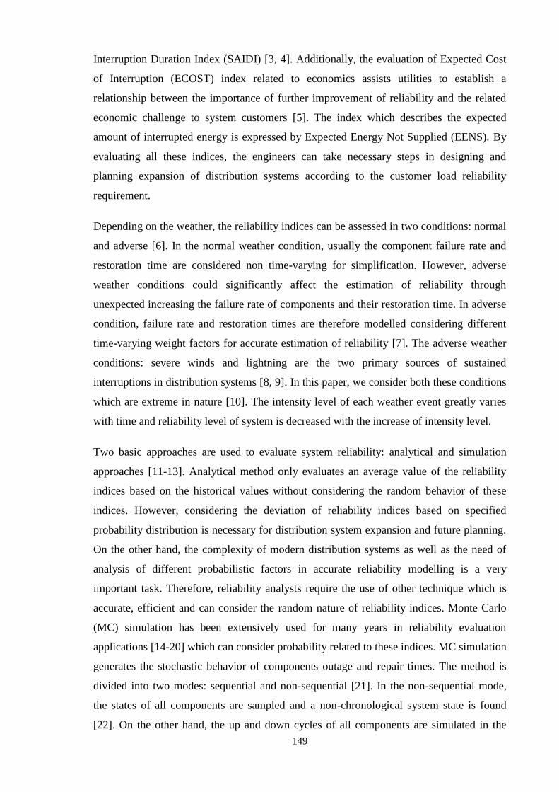
149

Interruption Duration Index (SAIDI) [3, 4]. Additionally, the evaluation of Expected Cost

of Interruption (ECOST) index related to economics assists utilities to establish a

relationship between the importance of further improvement of reliability and the related

economic challenge to system customers [5]. The index which describes the expected

amount of interrupted energy is expressed by Expected Energy Not Supplied (EENS). By

evaluating all these indices, the engineers can take necessary steps in designing and

planning expansion of distribution systems according to the customer load reliability

requirement.

Depending on the weather, the reliability indices can be assessed in two conditions: normal

and adverse [6]. In the normal weather condition, usually the component failure rate and

restoration time are considered non time-varying for simplification. However, adverse

weather conditions could significantly affect the estimation of reliability through

unexpected increasing the failure rate of components and their restoration time. In adverse

condition, failure rate and restoration times are therefore modelled considering different

time-varying weight factors for accurate estimation of reliability [7]. The adverse weather

conditions: severe winds and lightning are the two primary sources of sustained

interruptions in distribution systems [8, 9]. In this paper, we consider both these conditions

which are extreme in nature [10]. The intensity level of each weather event greatly varies

with time and reliability level of system is decreased with the increase of intensity level.

Two basic approaches are used to evaluate system reliability: analytical and simulation

approaches [11-13]. Analytical method only evaluates an average value of the reliability

indices based on the historical values without considering the random behavior of these

indices. However, considering the deviation of reliability indices based on specified

probability distribution is necessary for distribution system expansion and future planning.

On the other hand, the complexity of modern distribution systems as well as the need of

analysis of different probabilistic factors in accurate reliability modelling is a very

important task. Therefore, reliability analysts require the use of other technique which is

accurate, efficient and can consider the random nature of reliability indices. Monte Carlo

(MC) simulation has been extensively used for many years in reliability evaluation

applications [14-20] which can consider probability related to these indices. MC simulation

generates the stochastic behavior of components outage and repair times. The method is

divided into two modes: sequential and non-sequential [21]. In the non-sequential mode,

the states of all components are sampled and a non-chronological system state is found

[22]. On the other hand, the up and down cycles of all components are simulated in the

150

sequential form and overall system operating cycle is achieved by combining all the

components cycles [22]. The sequential MC allows the consideration of the chronological

matters and distributions of the reliability indices [23]. The state duration sampling

approach is generally used to simulate chronological issues which can describe time-

related reliability indices concerning frequency and duration of interruption [24]. However,

the sequential MC simulation significantly decreases the computational efficiency and

practicability when dealing with very reliable system with probabilities of very smaller

occurrence (i.e. high accuracy).

Over the years, several advanced various variance reduction techniques (VRT) have been

applied to enhance its convergence speed of the MC method. Through VRT, the expected

value of an output random variable can be obtained with reduced computation time by

maintaining a pre-defined level of accuracy. VRT based on cross-entropy method,

importance sampling approach has been utilized extensively in power system reliability

applications in order to speedup computation which are mainly carried out on the

generation and transmission systems reliability evaluation [25-28]. There has been a lack

of research in the area of distribution systems reliability assessment by applying these

advanced MCS methods. Another issue is to incorporate weather condition which has an

effect on the computation. It should be noted that the aim of this paper is not to develop

new models of weather-dependent failure rate and restoration time. However the purpose

of this paper is to demonstrate the practicality of the novel Multilevel Monte Carlo

(MLMC) simulation technique in distribution system reliability evaluation under different

weather conditions.

The MLMC simulation approach is an advanced MC method which has been recently

developed by Giles [29]. In MC method, the accuracy of the output variable is high since a

large number of iterations is run only on the finest grid level [30] which requires high

computation time. In MLMC simulation, a series of coarse levels is used to achieve the

finest level accuracy [31]. On each level, expectations are estimated using different sample

size in a manner which could decrease the overall variance for a pre-defined error

tolerance. Through performing simulations on multiple discretisation time-steps, less

number of samples is required on the expensive finest level in MLMC than MC to achieve

the same accuracy. Since a sequence of levels is used therefore less precise estimation on

the previous coarse level can be sequentially corrected by estimation on the next fine levels

[29].

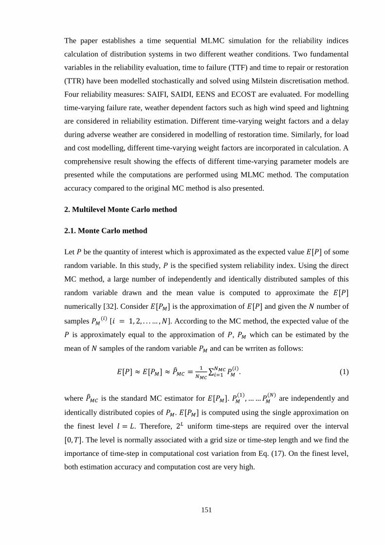
151

The paper establishes a time sequential MLMC simulation for the reliability indices

calculation of distribution systems in two different weather conditions. Two fundamental

variables in the reliability evaluation, time to failure (TTF) and time to repair or restoration

(TTR) have been modelled stochastically and solved using Milstein discretisation method.

Four reliability measures: SAIFI, SAIDI, EENS and ECOST are evaluated. For modelling

time-varying failure rate, weather dependent factors such as high wind speed and lightning

are considered in reliability estimation. Different time-varying weight factors and a delay

during adverse weather are considered in modelling of restoration time. Similarly, for load

and cost modelling, different time-varying weight factors are incorporated in calculation. A

comprehensive result showing the effects of different time-varying parameter models are

presented while the computations are performed using MLMC method. The computation

accuracy compared to the original MC method is also presented.

2. Multilevel Monte Carlo method

2.1. Monte Carlo method

Let be the quantity of interest which is approximated as the expected value of some

random variable. In this study, is the specified system reliability index. Using the direct

MC method, a large number of independently and identically distributed samples of this

random variable drawn and the mean value is computed to approximate the

numerically [32]. Consider is the approximation of and given the number of

samples [ ]. According to the MC method, the expected value of the

is approximately equal to the approximation of , which can be estimated by the

mean of samples of the random variable and can be wrriten as follows:

(1)

where is the standard MC estimator for .

are independently and

identically distributed copies of . is computed using the single approximation on

the finest level . Therefore, uniform time-steps are required over the interval

. The level is normally associated with a grid size or time-step length and we find the

importance of time-step in computational cost variation from Eq. (17). On the finest level,

both estimation accuracy and computation cost are very high.

152

The accuracy of this estimation can be quantified using the mean square error (MSE) of the

estimator which is denoted by . Since all the simulations are carried out on the level

therefore, it reduces the discretisation error but increases the simulation running

time. The variance of the MC estimator is

. To achieve an accuracy

level of , the simulation requires samples which needs huge computation

time. This is especially true when dealing with rare events. In term of computational

complexity, the estimated cost related to this estimator can be written as:

(2)

where is the computation cost for one sample of and estimated as for a

constant and some . is the cost refinement factor used to refine the time-step at

each level [30]. For both MC and MLMC methods, is considered which means each

level has twice as many time-steps as the prior level. is the rate of cost increase with the

increase of . An effective numerical solver usually provides a small . The value of can

be determined by fitting the curve of with varies of . The smaller values of and

reduce the cost of the estimator, but increase MSE. Therefore, in order to reduce the cost

without altering the level of accuracy, an efficient estimator is required.

2.2. MLMC approach

2.2.1. Basics of MLMC method

MLMC approach is a VRT for the MC simulation. The basic idea of MLMC method is to

use multigrid through a geometric order of levels starting from the coarsest grid to finest

grid. Such as the target is estimated through sum of multiple which are run on a

series of levels as . and are the coarsest and finest levels,

respectively. In stochastic modeling of reliability index using SDE, single time-step is used

for simulations on . On the other hand, uniform time-steps are required on .

On the coarsest level, both accuracy and required computation time are least and on the

finest level, both are highest. The cost is proportional to the total number of time-steps

particularly the computation time increases greatly for large number of the finest level

samples. Initially the expected value on , is estimated using number of time-

step and then correction value of reliability estimation is estimated as

on levels using different number of time-steps ,

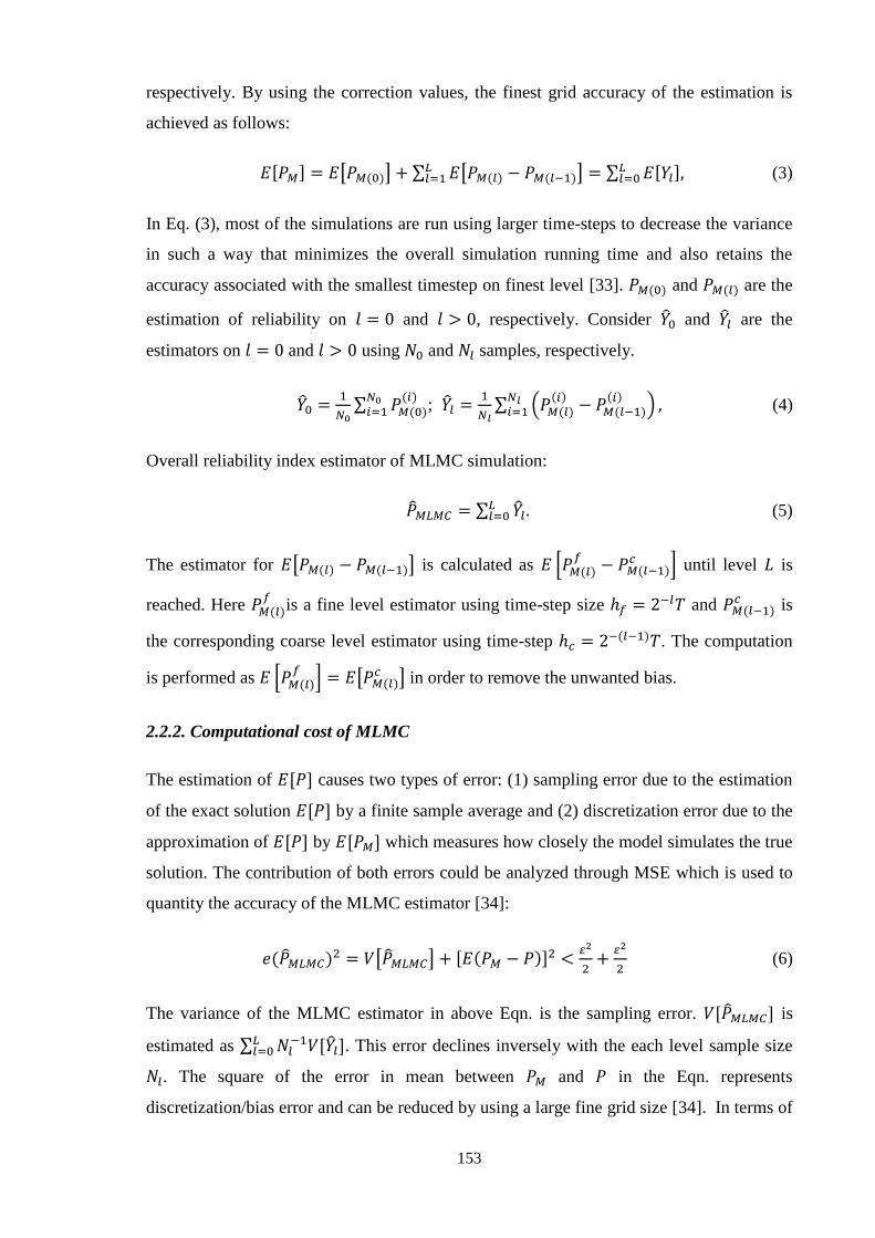
153

respectively. By using the correction values, the finest grid accuracy of the estimation is

achieved as follows:

(3)

In Eq. (3), most of the simulations are run using larger time-steps to decrease the variance

in such a way that minimizes the overall simulation running time and also retains the

accuracy associated with the smallest timestep on finest level [33]. and are the

estimation of reliability on and , respectively. Consider and are the

estimators on and using and samples, respectively.

;

(4)

Overall reliability index estimator of MLMC simulation:

(5)

The estimator for is calculated as

until level is

reached. Here

is a fine level estimator using time-step size and is

the corresponding coarse level estimator using time-step . The computation

is performed as

in order to remove the unwanted bias.

2.2.2. Computational cost of MLMC

The estimation of causes two types of error: (1) sampling error due to the estimation

of the exact solution by a finite sample average and (2) discretization error due to the

approximation of by which measures how closely the model simulates the true

solution. The contribution of both errors could be analyzed through MSE which is used to

quantity the accuracy of the MLMC estimator [34]:

(6)

The variance of the MLMC estimator in above Eqn. is the sampling error. is

estimated as

. This error declines inversely with the each level sample size

. The square of the error in mean between and in the Eqn. represents

discretization/bias error and can be reduced by using a large fine grid size [34]. In terms of

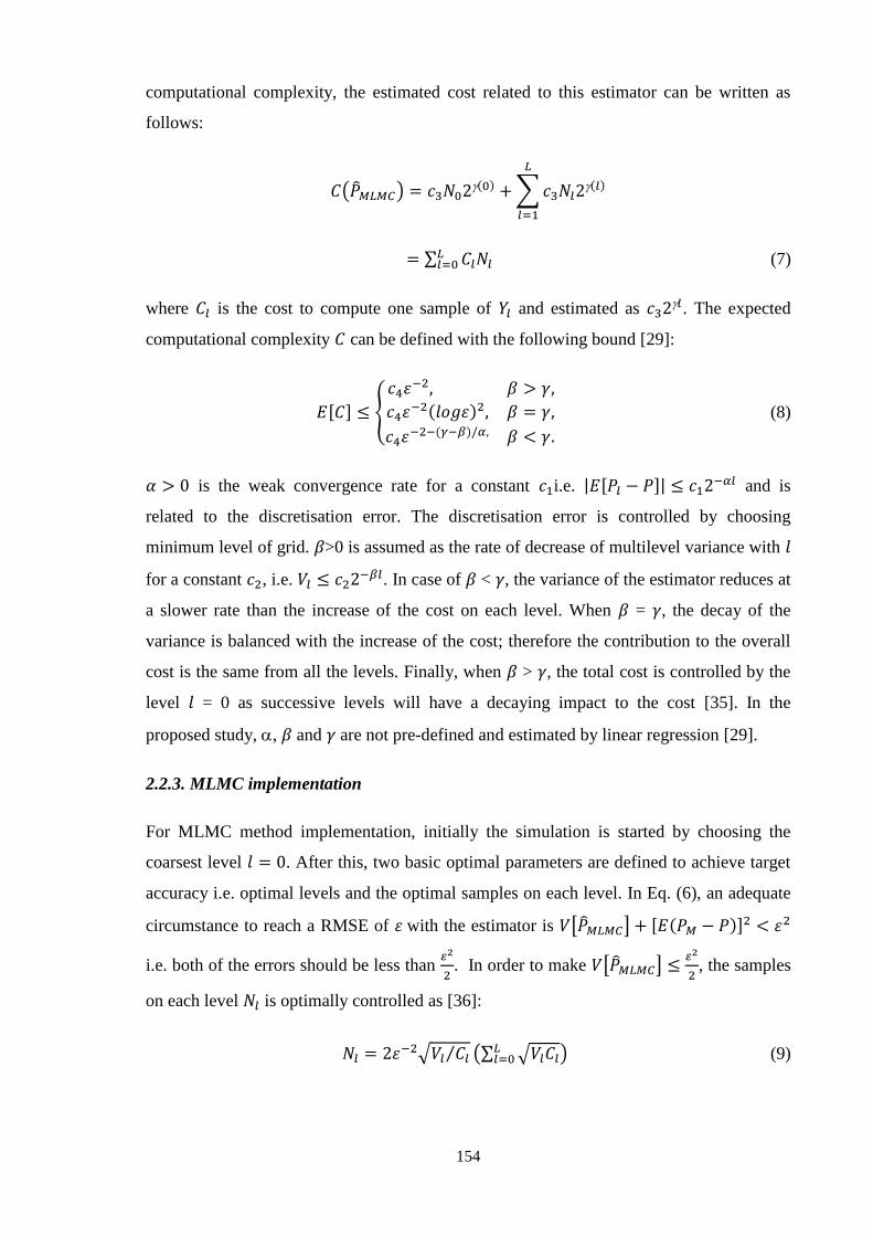
154

computational complexity, the estimated cost related to this estimator can be written as

follows:

(7)

where is the cost to compute one sample of and estimated as . The expected

computational complexity can be defined with the following bound [29]:

(8)

is the weak convergence rate for a constant i.e. and is

related to the discretisation error. The discretisation error is controlled by choosing

minimum level of grid. >0 is assumed as the rate of decrease of multilevel variance with

for a constant , i.e. . In case of < , the variance of the estimator reduces at

a slower rate than the increase of the cost on each level. When = , the decay of the

variance is balanced with the increase of the cost; therefore the contribution to the overall

cost is the same from all the levels. Finally, when > , the total cost is controlled by the

level = 0 as successive levels will have a decaying impact to the cost [35]. In the

proposed study, , and are not pre-defined and estimated by linear regression [29].

2.2.3. MLMC implementation

For MLMC method implementation, initially the simulation is started by choosing the

coarsest level . After this, two basic optimal parameters are defined to achieve target

accuracy i.e. optimal levels and the optimal samples on each level. In Eq. (6), an adequate

circumstance to reach a RMSE of with the estimator is

i.e. both of the errors should be less than

. In order to make

, the samples

on each level is optimally controlled as [36]:

(9)

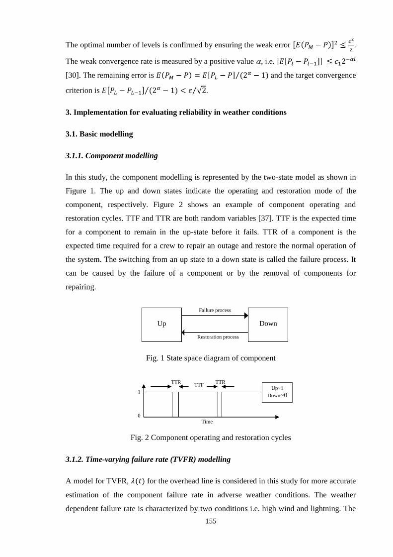
155

The optimal number of levels is confirmed by ensuring the weak error

.

The weak convergence rate is measured by a positive value , i.e.

[30]. The remaining error is and the target convergence

criterion is .

3. Implementation for evaluating reliability in weather conditions

3.1. Basic modelling

3.1.1. Component modelling

In this study, the component modelling is represented by the two-state model as shown in

Figure 1. The up and down states indicate the operating and restoration mode of the

component, respectively. Figure 2 shows an example of component operating and

restoration cycles. TTF and TTR are both random variables [37]. TTF is the expected time

for a component to remain in the up-state before it fails. TTR of a component is the

expected time required for a crew to repair an outage and restore the normal operation of

the system. The switching from an up state to a down state is called the failure process. It

can be caused by the failure of a component or by the removal of components for

repairing.

Fig. 1 State space diagram of component

Fig. 2 Component operating and restoration cycles

3.1.2. Time-varying failure rate (TVFR) modelling

A model for TVFR, for the overhead line is considered in this study for more accurate

estimation of the component failure rate in adverse weather conditions. The weather

dependent failure rate is characterized by two conditions i.e. high wind and lightning. The

0

TTR TTF

TTR Up~1

Down~0

Time

1

Restoration process

Failure process

Up

Down

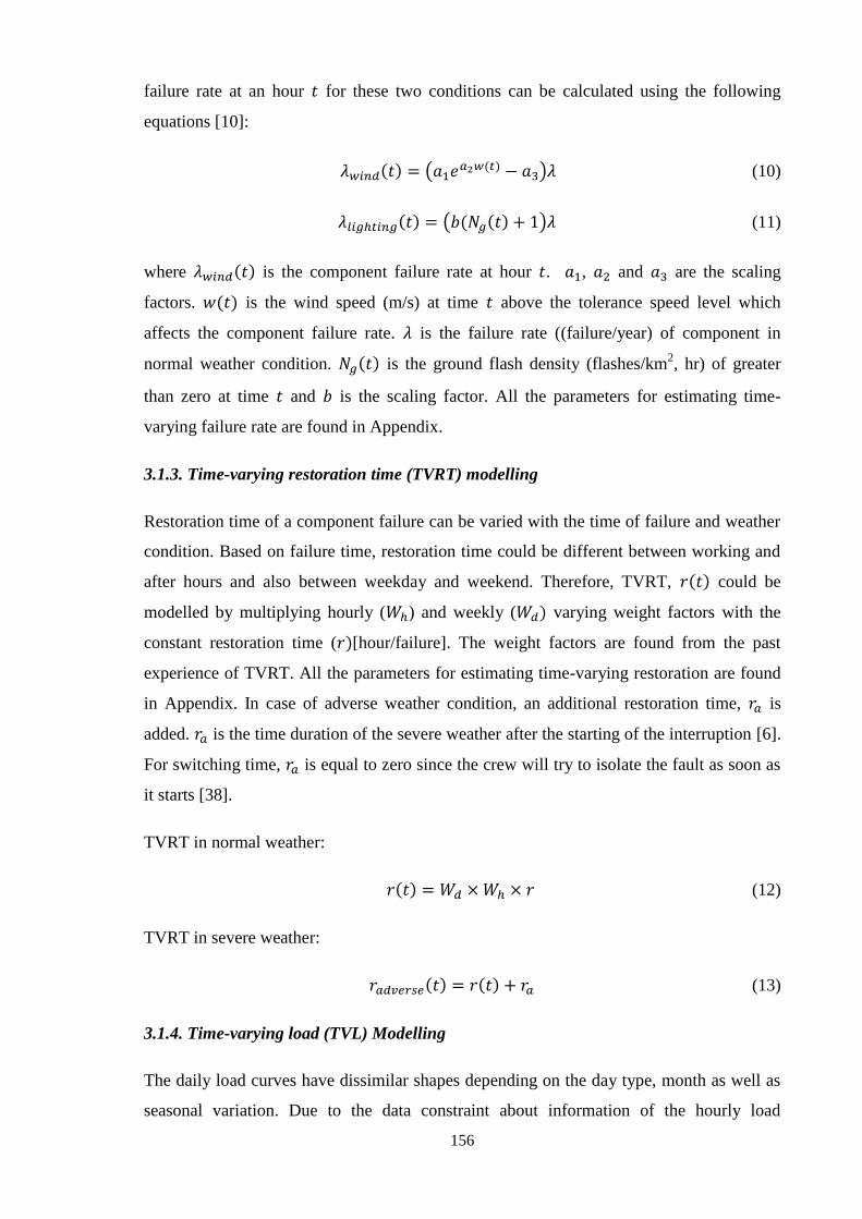
156

failure rate at an hour for these two conditions can be calculated using the following

equations [10]:

(10)

(11)

where is the component failure rate at hour . , and are the scaling

factors. is the wind speed (m/s) at time above the tolerance speed level which

affects the component failure rate. is the failure rate ((failure/year) of component in

normal weather condition. is the ground flash density (flashes/km2, hr) of greater

than zero at time and is the scaling factor. All the parameters for estimating time-

varying failure rate are found in Appendix.

3.1.3. Time-varying restoration time (TVRT) modelling

Restoration time of a component failure can be varied with the time of failure and weather

condition. Based on failure time, restoration time could be different between working and

after hours and also between weekday and weekend. Therefore, TVRT, could be

modelled by multiplying hourly ( ) and weekly ( varying weight factors with the

constant restoration time ( [hour/failure]. The weight factors are found from the past

experience of TVRT. All the parameters for estimating time-varying restoration are found

in Appendix. In case of adverse weather condition, an additional restoration time, is

added. is the time duration of the severe weather after the starting of the interruption [6].

For switching time, is equal to zero since the crew will try to isolate the fault as soon as

it starts [38].

TVRT in normal weather:

(12)

TVRT in severe weather:

(13)

3.1.4. Time-varying load (TVL) Modelling

The daily load curves have dissimilar shapes depending on the day type, month as well as

seasonal variation. Due to the data constraint about information of the hourly load

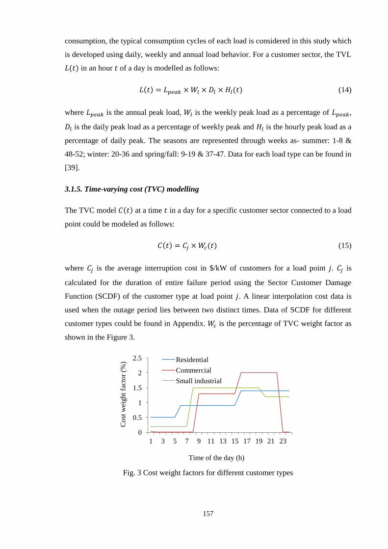
157

consumption, the typical consumption cycles of each load is considered in this study which

is developed using daily, weekly and annual load behavior. For a customer sector, the TVL

in an hour of a day is modelled as follows:

(14)

where is the annual peak load, is the weekly peak load as a percentage of ,

is the daily peak load as a percentage of weekly peak and is the hourly peak load as a

percentage of daily peak. The seasons are represented through weeks as- summer: 1-8 &

48-52; winter: 20-36 and spring/fall: 9-19 & 37-47. Data for each load type can be found in

[39].

3.1.5. Time-varying cost (TVC) modelling

The TVC model at a time in a day for a specific customer sector connected to a load

point could be modeled as follows:

(15)

where is the average interruption cost in $/kW of customers for a load point . is

calculated for the duration of entire failure period using the Sector Customer Damage

Function (SCDF) of the customer type at load point . A linear interpolation cost data is

used when the outage period lies between two distinct times. Data of SCDF for different

customer types could be found in Appendix. is the percentage of TVC weight factor as

shown in the Figure 3.

Fig. 3 Cost weight factors for different customer types

0

0.5

1

1.5

2

2.5

1 3 5 7 9 11 13 15 17 19 21 23

Co

st w

eigh

t fa

ctor

(%)

Time of the day (h)

Residential

Commercial

Small industrial

158

3.1.6. Modelling of time-varying system reliability

For modelling system reliability, two basic random variables of each component i.e. TTF

and TTR are initially modelled. Note that the time of an outage event is absolutely random

and there is no such guarantee that a component will follow the outage history of the

similar elements. Therefore, TTF and TTR of an outage event are random variables and

just approximations of the actual TTF and TTR, respectively. In this study, we model TTF

and TTR using SDE which is driven by Brownian motion where the outputs are normally

distributed random variables. Consider, and represent constant failure rate and repair

time of a component i, respectively. Then the SDE of TTF for this component on the time

[ ] can be expressed as follows [40, 41]:

(16)

where is the TTF at a time with an initial TTF of in normal

weather. For an adverse weather, initial TTF is defined by Eqs. (10) or (11) based on

condition.

The rate of change of average value of stochastic process and the degree of variation of

stochastic process over time are denoted as and , respectively. The SDE of TTF can be

solved by using a discretisation scheme [42] and here we use Milstein discretisation [43].

The Milstein discretisation with number of time-steps, step size and Brownian

increments is [44]

(17)

where , ; ,

; are independently and normally distributed random

variables.

Reliability of a distribution system is typically assessed with the useful life period of the

component and the failure rate is assumed constant [45]. The operating history ( of a

component is generated in a sequential way based on random sampling method from the

exponential probability distribution of component TTF [46, 47]. Now of component

can be generated as:

(18)

159


Using the similar procedure, the artificial restoration history of each component is

generated. For SDE of TTR, and are considered equal as TTF. The initial TVRT,

for component during normal weather condition, . where is a constant for

component and . For an adverse condition, is replaced by

and is redefined based on Eqs. (10) or (11).

of component can be generated as:

(19)


The average failure rate, and average unavailability, for a component can be

calculated as:

(outage/year) (20)

(hour/year) (21)

where is the number of times component fails during entire simulation time and N is

the desired number of simulated periods. In Eq. (21), the denominator is divided by

8760 to convert its unit from hour to year. Average failure rate, and annual

unavailability, for a load point could be calculated as follows:

(interruption/year) (22)

(hour/year) (23)

where denotes the number of outage events affecting the service of load point .

The reliability indices considering the time-varying parameter models can be modelled as

follows:

(failure/system customer per year) (24)

160

(hour/ system customer per year) (25)

(k$/year) (26)

(MWh/year) (27)

where is the total number of supply points. is the number of customers at point

and is the total number of customers served. and are the time-varying load and

cost levels, respectively and estimated as follows:

;

(28)

where and are the failure start and end hours, respectively.

3.2. Summary of simulation procedure to estimate reliability

Using the proposed method, the reliability evaluation methodology consists by the

following steps. Steps (1)-(8) describe the mathematical modelling of index on both coarse

and fine grid levels and then steps (9)-(13) describe the convergence test process in the

estimation.

(1) Define the input of reliability estimation. The input data include failure rate, repair time

of each component failure event, sample size for convergence test ( ), the initial sample

size on each level ( ) and the time-varying weight factors as described from section 3.1 to

3.4.

(2) Formulate the stochastic TTF models for a failed component on the coarse and find

levels using Milstein method as follows.

(29)

(30)

where and are the time-step sizes for coarse and fine path estimators which can be

expressed as and respectively.

161

(3) Using the corresponding SDE of TTF, the operating ( and restoration histories

( of component are generated on coarse and fine levels.

;

(31)

;

(32)

(4) Calculate component and on both levels using the corresponding operating and

restoration histories as follows:

;

(33)

;

(34)

For each component failure, steps (2)-(4) are repeated.

(5) Find the load points interrupted by component failure and calculate and on both

levels using components indices.

;

(35)

;

(36)

(6) Repeat steps (2)-(5) for each load point in the system.

(7) Estimate the system reliability indices on both coarse and fine levels as follows:

;

;

;

. (37)

;

;

;

.(38)

(8) Using coarse and fine levels reliability index values, calculate the sum on levels

and . The simulation is repeated until the number of samples is reached to .

(9) For convergence test, the initial value of the finest level is set at .

162

(10) Generate the number of samples on using and also update the sum

from step (8).

(11) Calculate the absolute mean and variance on each level .

(12) Find out the optimal number of samples on each level using Eq. (9) and evaluate

extra samples if needed by comparing with . Moreover, update mean and variance on

each level for confirming variance of the MLMC

(13) If not converged, set and test convergence again until reached to the target

accuracy level. Finally, calculate the multilevel estimator using Eq. (5).

3.3. Test System

A very well-known reliability test system called RBTS Bus 4 [48] as shown in Figure 4 is

used as test distribution system. The test system is generally developed by considering all

the actual complexities of a practical distribution system. It is a complex urban type

network and consists of 38 supply points with commercial, residential and industrial

customers. Component reliability data for the system are found in [49]. The customer data,

load data and types, feeder and length data are provided in Appendix D. The availability

and reliability of breakers, fuses and disconnecting switches are considered 100%. The

availability of alternative supply source is also considered. The service of failed low

voltage transformers is restored by repairing rather than replacing.

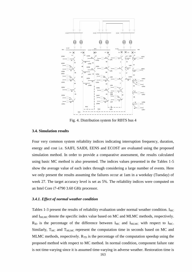
163

N/O

45

46

47

48

33 kV33 kV33 kV

11 kV11 kV

11 kV

F3F2F1F7F6F5F4

1913150

4431

20

21

22

23

24

25

26

27

28

29

30

14

15

16

17

18

2

3

4

5

6

7

8

9

10

11

12

57

58

59

60

61

62

63

64

65

66

67

51

52

53

54

55

49

32

33

34

35

36

37

38

39

40

41

42

43

LP11

LP12

LP13

LP14

LP15

LP16

LP17

LP8

LP9

LP10

56

LP1

LP2

LP3

LP4

LP5

LP6

LP7

LP32

LP33

LP34

LP35

LP36

LP37

LP38

LP29

LP30

LP31

LP26

LP27

LP28

LP18

LP19

LP20

LP21

LP22

LP23

LP24

LP25

N/O

N/O

N/O

SP1SP2SP3

Fig. 4. Distribution system for RBTS bus 4

3.4. Simulation results

Four very common system reliability indices indicating interruption frequency, duration,

energy and cost i.e. SAIFI, SAIDI, EENS and ECOST are evaluated using the proposed

simulation method. In order to provide a comparative assessment, the results calculated

using basic MC method is also presented. The indices values presented in the Tables 1-5

show the average value of each index through considering a large number of events. Here

we only present the results assuming the failures occur at 1am in a weekday (Tuesday) of

week 27. The target accuracy level is set as 5%. The reliability indices were computed on

an Intel Core i7‐4790 3.60 GHz processor.

3.4.1. Effect of normal weather condition

Tables 1-3 present the results of reliability evaluation under normal weather condition. IMC

and IMLMC denote the specific index value based on MC and MLMC methods, respectively.

RID is the percentage of the difference between IMC and IMLMC with respect to IMC.

Similarly, TMC and TMLMC represent the computation time in seconds based on MC and

MLMC methods, respectively. RTD is the percentage of the computation speedup using the

proposed method with respect to MC method. In normal condition, component failure rate

is not time-varying since it is assumed time-varying in adverse weather. Restoration time is

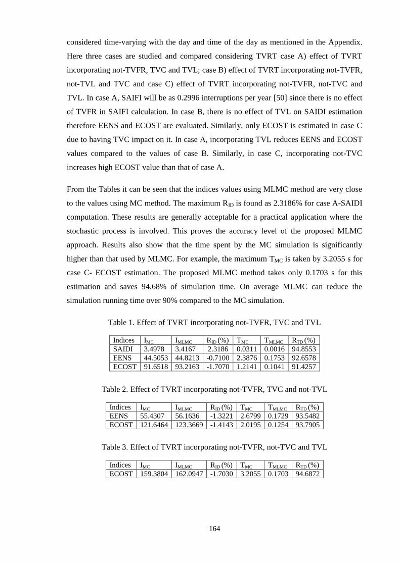
164

considered time-varying with the day and time of the day as mentioned in the Appendix.

Here three cases are studied and compared considering TVRT case A) effect of TVRT

incorporating not-TVFR, TVC and TVL; case B) effect of TVRT incorporating not-TVFR,

not-TVL and TVC and case C) effect of TVRT incorporating not-TVFR, not-TVC and

TVL. In case A, SAIFI will be as 0.2996 interruptions per year [50] since there is no effect

of TVFR in SAIFI calculation. In case B, there is no effect of TVL on SAIDI estimation

therefore EENS and ECOST are evaluated. Similarly, only ECOST is estimated in case C

due to having TVC impact on it. In case A, incorporating TVL reduces EENS and ECOST

values compared to the values of case B. Similarly, in case C, incorporating not-TVC

increases high ECOST value than that of case A.

From the Tables it can be seen that the indices values using MLMC method are very close

to the values using MC method. The maximum RID is found as 2.3186% for case A-SAIDI

computation. These results are generally acceptable for a practical application where the

stochastic process is involved. This proves the accuracy level of the proposed MLMC

approach. Results also show that the time spent by the MC simulation is significantly

higher than that used by MLMC. For example, the maximum TMC is taken by 3.2055 s for

case C- ECOST estimation. The proposed MLMC method takes only 0.1703 s for this

estimation and saves 94.68% of simulation time. On average MLMC can reduce the

simulation running time over 90% compared to the MC simulation.

Table 1. Effect of TVRT incorporating not-TVFR, TVC and TVL

Indices IMC IMLMC RID (%) TMC TMLMC RTD (%)

SAIDI 3.4978 3.4167 2.3186 0.0311 0.0016 94.8553

EENS 44.5053 44.8213 -0.7100 2.3876 0.1753 92.6578

ECOST 91.6518 93.2163 -1.7070 1.2141 0.1041 91.4257

Table 2. Effect of TVRT incorporating not-TVFR, TVC and not-TVL

Table 3. Effect of TVRT incorporating not-TVFR, not-TVC and TVL


EENS 55.4307 56.1636 -1.3221 2.6799 0.1729 93.5482

ECOST 121.6464 123.3669 -1.4143 2.0195 0.1254 93.7905


ECOST 159.3804 162.0947 -1.7030 3.2055 0.1703 94.6872

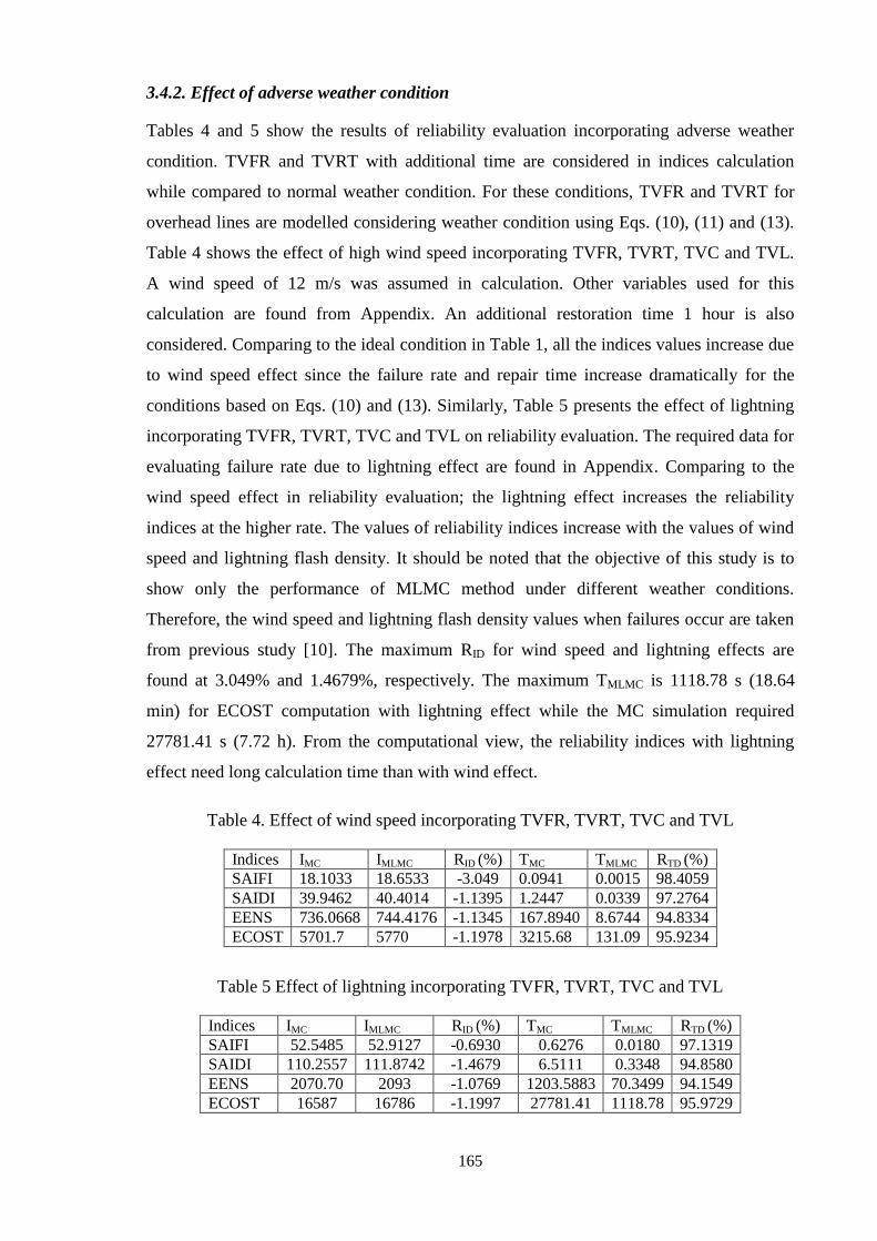
165

3.4.2. Effect of adverse weather condition

Tables 4 and 5 show the results of reliability evaluation incorporating adverse weather

condition. TVFR and TVRT with additional time are considered in indices calculation

while compared to normal weather condition. For these conditions, TVFR and TVRT for

overhead lines are modelled considering weather condition using Eqs. (10), (11) and (13).

Table 4 shows the effect of high wind speed incorporating TVFR, TVRT, TVC and TVL.

A wind speed of 12 m/s was assumed in calculation. Other variables used for this

calculation are found from Appendix. An additional restoration time 1 hour is also

considered. Comparing to the ideal condition in Table 1, all the indices values increase due

to wind speed effect since the failure rate and repair time increase dramatically for the

conditions based on Eqs. (10) and (13). Similarly, Table 5 presents the effect of lightning

incorporating TVFR, TVRT, TVC and TVL on reliability evaluation. The required data for

evaluating failure rate due to lightning effect are found in Appendix. Comparing to the

wind speed effect in reliability evaluation; the lightning effect increases the reliability

indices at the higher rate. The values of reliability indices increase with the values of wind

speed and lightning flash density. It should be noted that the objective of this study is to

show only the performance of MLMC method under different weather conditions.

Therefore, the wind speed and lightning flash density values when failures occur are taken

from previous study [10]. The maximum RID for wind speed and lightning effects are

found at 3.049% and 1.4679%, respectively. The maximum TMLMC is 1118.78 s (18.64

min) for ECOST computation with lightning effect while the MC simulation required

27781.41 s (7.72 h). From the computational view, the reliability indices with lightning

effect need long calculation time than with wind effect.

Table 4. Effect of wind speed incorporating TVFR, TVRT, TVC and TVL


SAIFI 18.1033 18.6533 -3.049 0.0941 0.0015 98.4059

SAIDI 39.9462 40.4014 -1.1395 1.2447 0.0339 97.2764

EENS 736.0668 744.4176 -1.1345 167.8940 8.6744 94.8334

ECOST 5701.7 5770 -1.1978 3215.68 131.09 95.9234

Table 5 Effect of lightning incorporating TVFR, TVRT, TVC and TVL


SAIFI 52.5485 52.9127 -0.6930 0.6276 0.0180 97.1319

SAIDI 110.2557 111.8742 -1.4679 6.5111 0.3348 94.8580

EENS 2070.70 2093 -1.0769 1203.5883 70.3499 94.1549

ECOST 16587 16786 -1.1997 27781.41 1118.78 95.9729

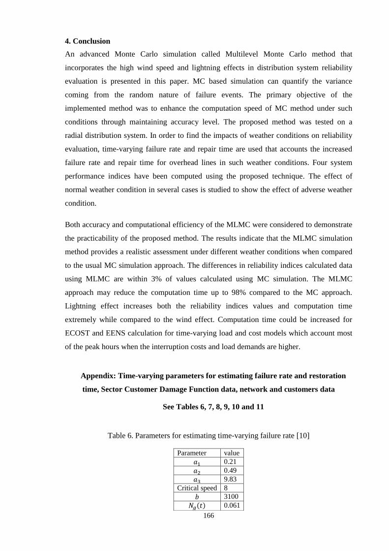
166

4. Conclusion

An advanced Monte Carlo simulation called Multilevel Monte Carlo method that

incorporates the high wind speed and lightning effects in distribution system reliability

evaluation is presented in this paper. MC based simulation can quantify the variance

coming from the random nature of failure events. The primary objective of the

implemented method was to enhance the computation speed of MC method under such

conditions through maintaining accuracy level. The proposed method was tested on a

radial distribution system. In order to find the impacts of weather conditions on reliability

evaluation, time-varying failure rate and repair time are used that accounts the increased

failure rate and repair time for overhead lines in such weather conditions. Four system

performance indices have been computed using the proposed technique. The effect of

normal weather condition in several cases is studied to show the effect of adverse weather

condition.

Both accuracy and computational efficiency of the MLMC were considered to demonstrate

the practicability of the proposed method. The results indicate that the MLMC simulation

method provides a realistic assessment under different weather conditions when compared

to the usual MC simulation approach. The differences in reliability indices calculated data

using MLMC are within 3% of values calculated using MC simulation. The MLMC

approach may reduce the computation time up to 98% compared to the MC approach.

Lightning effect increases both the reliability indices values and computation time

extremely while compared to the wind effect. Computation time could be increased for

ECOST and EENS calculation for time-varying load and cost models which account most

of the peak hours when the interruption costs and load demands are higher.

Appendix: Time-varying parameters for estimating failure rate and restoration

time, Sector Customer Damage Function data, network and customers data

See Tables 6, 7, 8, 9, 10 and 11

Table 6. Parameters for estimating time-varying failure rate [10]

Parameter value

0.21

0.49

9.83

Critical speed 8

3100

0.061

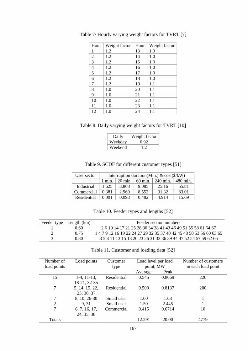
167

Table 7/ Hourly varying weight factors for TVRT [7]

Hour Weight factor Hour Weight factor

1 1.2 13 1.0

2 1.2 14 1.0

3 1.2 15 1.0

4 1.2 16 1.0

5 1.2 17 1.0

6 1.2 18 1.0

7 1.2 19 1.1

8 1.0 20 1.1

9 1.0 21 1.1

10 1.0 22 1.1

11 1.0 23 1.1

12 1.0 24 1.1

Table 8. Daily varying weight factors for TVRT [10]

Daily Weight factor

Weekday 0.92

Weekend 1.2

Table 9. SCDF for different customer types [51]

User sector Interruption duration(Min.) & cost($/kW)

1 min. 20 min. 60 min. 240 min. 480 min.

Industrial 1.625 3.868 9.085 25.16 55.81

Commercial 0.381 2.969 8.552 31.32 83.01

Residential 0.001 0.093 0.482 4.914 15.69

Table 10. Feeder types and lengths [52]

Feeder type Length (km) Feeder section numbers

1 0.60 2 6 10 14 17 21 25 28 30 34 38 41 43 46 49 51 55 58 61 64 67

2 0.75 1 4 7 9 12 16 19 22 24 27 29 32 35 37 40 42 45 48 50 53 56 60 63 65

3 0.80 3 5 8 11 13 15 18 20 23 26 31 33 36 39 44 47 52 54 57 59 62 66

Table 11. Customer and loading data [52]

Number of

load points

Load points Customer

type

Load level per load

point, MW

Number of customers

in each load point

Average Peak

15 1-4, 11-13,

18-21, 32-35

Residential 0.545 0.8669 220

7 5, 14, 15, 22,

23, 36, 37

Residential 0.500 0.8137 200

7 8, 10, 26-30 Small user 1.00 1.63 1

2 9, 31 Small user 1.50 2.445 1

7 6, 7, 16, 17,

24, 35, 38

Commercial 0.415 0.6714 10

Totals 12.291 20.00 4779

168

References

1. Billinton R, Allan RN (1994) Reliability evaluation of power systems: Plenum Publishing

(New York).

2. Billinton R, Billinton JE (1989) Distribution system reliability indices. IEEE Trans Power

Del 4(1):561-568.

3. Goel L, Billinton R (1991) Evaluation of interrupted energy assessment rates in

distribution systems. IEEE Trans Power Del 6(4):1876-1882.

4. Sultana B, Mustafa M, Sultana U, Bhatti AR (2016) Review on reliability improvement

and power loss reduction in distribution system via network reconfiguration.

Renew Sustain Energy Rev 66: 297-310.

5. Goel L (1998) Power system reliability cost/benefit assessment and application in

perspective. Comput Electr Eng 24(5):315-324.

6. Alvehag K, L. Soder (2008) A stochastic weather dependent reliability model for

distribution systems. In: Proceedings of the IEEE 10th international conference on

probabilistic methods applied to power systems, pp 1-8.

7. Wang P, Billinton R (2002) Reliability cost/worth assessment of distribution systems

incorporating time-varying weather conditions and restoration resources. IEEE Trans

Power Del 17(1): 260-265.

8. Darveniza M, Arnold C, Holcombe B, Rainbird P (2007) The relationships between

weather variables and reliability indices for a distribution system in South-East

Queensland. In: Proceedings of international conference on electricity distribution, Vienna,

Austria.

9. Pahwa A, Hopkins M, Gaunt T (2007) Evaluation of outages in overhead distribution

systems of south africa and of Manhattan, Kansas, USA. In: Proceedings of international

conference on power systems operation and planning, Cape Town, South Africa.

10. Alvehag K. Soder L (2011) A reliability model for distribution systems incorporating

seasonal variations in severe weather. IEEE Trans Power Del 26(2): 910-919.

11. Ou Y, Goel L (1999) Using Monte Carlo simulation for overall distribution system

reliability worth assessment. IET Gener. Transm. Distrib 146(5): 535-540.

12. Billinton R, Wang P (1998) Distribution system reliability cost/worth analysis using

analytical and sequential simulation techniques. IEEE Trans Power Syst 13(4): 1245-1250.

13. Volkanovski A, Čepin M, Mavko B (2009) Application of the fault tree analysis for

assessment of power system reliability. Reliab Eng Syst Safe 94(6): 1116-1127.

169

14. Ou Y, Goel L (1999) Using Monte Carlo simulation for overall distribution system

reliability worth assessment. IET Gener. Transm. Distrib 146(5):535-540.

15. Goel L, Ou Y (1999) Reliability worth assessment in radial distribution systems using the

Monte Carlo simulation technique. Electr Power Syst Res 51(1): 43-53.

16. Goel L (2000) Monte Carlo simulation-based reliability studies of a distribution test

system. Electr Power Syst Res 54(1): 55-65.

17. Billinton R, Wang P (1999) Teaching distribution system reliability evaluation using

Monte Carlo simulation. IEEE Trans Power Syst 14(2): 397-403.

18. Hegazy Y, Salama M, Chikhani A (2003) Adequacy assessment of distributed generation

systems using Monte Carlo simulation. IEEE Trans Power Syst 18(1): 48-52.

19. Rocchetta R, Li Y, Zio E (2015) Risk assessment and risk-cost optimization of distributed

power generation systems considering extreme weather conditions. Reliab Eng Syst Safe

136: 47-61.

20. Goel L, Ou Y (2001) Radial distribution system reliability worth evaluation utilizing the

Monte Carlo simulation technique. Comput Electr Eng 27(3): 273-285.

21. Momoh JA (2007) Electric power distribution, automation, protection, and control: CRC

press.

22. Li W (2014) Risk assessment of power systems: models, methods, and applications: John

Wiley & Sons.

23. Billinton R, Sankarakrishnan A (1995). A comparison of Monte Carlo simulation

techniques for composite power system reliability assessment. In: Proceedings of the IEEE

communications, power, and computing. conference, vol 1, pp. 145-150.

24. Billinton R, Li W (1994) Distribution System and Station Adequacy Assessment, in

Reliability assessment of electric power systems using Monte Carlo methods. Springer:

209-254.

25. Hou K, Jia H, Xu X, Liu Z, Jiang Y (2016) A continuous time Markov chain based

sequential analytical approach for composite power system reliability assessment. IEEE

Trans Power Syst 31(1): 738-748.

26. González-Fernández RA, da Silva AML (2011) Reliability assessment of time-dependent

systems via sequential cross-entropy Monte Carlo simulation. IEEE Trans Power Syst

26(4): 2381-2389.

27. Wang Y, Guo C, Wu Q (2013) A cross-entropy-based three-stage sequential importance

sampling for composite power system short-term reliability evaluation. IEEE Trans Power

Syst 28(4): 4254-4263.

170

28. Huda ASN, Zivanovic R (2017) Accelerated Distribution Systems Reliability Evaluation

by Multilevel Monte Carlo Simulation: Implementation of Two Discretisation Schemes.

IET Gener. Transm. Distrib 11(13): 3397-3405.

29. Giles MB (2015). Multilevel Monte Carlo methods. Acta Numer 24: 259-328.

30. Giles MB (2008) Multilevel monte carlo path simulation. Oper. Res 56(3): p. 607-617.

31. Stuben K (2001) An introduction to algebraic multigrid. Multigrid: 413-532.

32. de Schryver C, Torruella P, When N (2013) A multi-level Monte Carlo FPGA accelerator

for option pricing in the Heston model. In: Proceedings of the Conference on design,

automation and test in Europe, pp. 248-253, EDA Consortium.

33. Giles M, Szpruch L (2013) Multilevel Monte Carlo methods for applications in finance.

Recent Advances in Computational Finance, World Scientific.

34. Cliffe K, Giles,M, Scheichl R, Teckentrup AL (2011) Multilevel Monte Carlo methods

and applications to elliptic PDEs with random coefficients. Computing and Visualization

in Science 14(1): 3-15.

35. Aslett LJ, Nagapetyan T, Vollmer SJ (2017) Multilevel Monte Carlo for reliability theory.

Reliab Eng Syst Safe 165: 188-196.

36. Elfverson D, Hellman F, Målqvist A (2014) A multilevel Monte Carlo method for

computing failure probabilities. arXiv preprint arXiv:1408.6856.

37. Billinton R, Wang P (1999) Teaching distribution system reliability evaluation using

Monte Carlo simulation. IEEE Trans Power Syst 14(2): p. 397-403.

38. Brown R, Gupta S, Christie R, Venkata S, Fletcher R (1997) Distribution system

reliability assessment: momentary interruptions and storms. IEEE Trans Power Del 12(4):

1569-1575.

39. Huda ASN, Živanović R (2018) Efficient estimation of interrupted energy with time-

varying load models for distribution systems planning studies. IFAC-PapersOnLine 51(2):

p. 208-213.

40. Oksendal B (2013) Stochastic differential equations: an introduction with applications:

Springer Science & Business Media.

41. Harrison JM (1985) Brownian motion and stochastic flow systems: Wiley New York.

42. Brugger C, de Schryver C, Wehn N, Omland S, Hefter M, Ritter K, Korn R (2014) Mixed

precision multilevel Monte Carlo on hybrid computing systems. In: Proceedings of IEEE

conference on computational intelligence for financial engineering & economics, pp. 215-

222.

43. Giles MB (2009) Multilevel Monte Carlo for basket options. In: Proceedings of the IEEE

Winter Simulation Conference (WSC), pp. 1283-1290.

171

44. Kloeden PE, Platen E (1992) Higher-order implicit strong numerical schemes for

stochastic differential equations. J. Stat. Phys 66(1-2): 283-314.

45. Chowdhury A, Koval D (2011) Power distribution system reliability: practical methods

and applications 48: John Wiley & Sons.

46. Wang P, Billinton R (2001) Time-sequential simulation technique for rural distribution

system reliability cost/worth evaluation including wind generation as alternative supply.

IET Gener. Transm. Distrib 148(4):355-360.

47. Billinton R, Allan RN (1992) Reliability evaluation of engineering systems: Springer.

48. Billinton R, Jonnavithula S (1996) A test system for teaching overall power system

reliability assessment. IEEE Trans Power Syst 11(4): 1670-1676.

49. Goel L, Billinton R, Gupta R (1991) Basic data and evaluation of distribution system

reliability worth. In: Proceedings of the IEEE Western Canada conference on computer,

power and communications systems in a rural environment, pp. 271-277.

50. Huda ASN, Živanović R (2017) Multilevel Monte Carlo simulation applied to distribution

systems reliability evaluation. In: Proceedings of the IEEE Manchester PowerTech, pp. 1-

6.

51. Wang P, Billinton R (1999) Time sequential distribution system reliability worth analysis

considering time varying load and cost models. IEEE Trans Power Del 14(3): 1046-1051.

52. Allan RN, Billinton R, Sjarief I, Goel L, So K (1991) A reliability test system for

educational purposes-basic distribution system data and results. IEEE Trans Power Syst

6(2): 813-820.

172

Chapter 8

Study of Large-Scale DG Integration into Distribution

Networks

173


Title of Paper Large scale penetration of distributed generation into distribution networks: Study objectives,

review of models and computational tools





manuscript style

Publication Details A.S.N. Huda and R. Živanović (2017) Large-scale penetration of distributed generation into

distribution networks: Study objectives, review of models and computational tools, Renewable

and Sustainable Energy Reviews, 76, 974-988.

Link: https://www.sciencedirect.com/science/article/pii/S1364032117303842

Principal author


(Candidate)

A. S. Nazmul Huda


Study objectives, review of models and computational tools and preparation of manuscript.





paper.








Contribution to the Paper Provided guidelines for manuscript writing, helped in manuscript edit and evaluation

Signature

Date 13.08.2018

https://www.sciencedirect.com/science/article/pii/S1364032117303842

174

Large-scale penetration of distributed generation into distribution networks: study

objectives, review of models and computational tools

Abstract- In terms of the improvement of reliability and efficiency, integration of

distributed generation (DG) into distribution network has gained significant interest in

recent years. However, existing distribution systems were not designed considering large-

scale penetration of DG. Due to the increasing penetration of DG, several technical

challenges may arise which includes voltage control, power quality and protection issues,

etc. Therefore, additional components need to be modelled together with conventional

distribution system components in order to study the impact of DG on the distribution

system. The first objective of this paper is to review the required models of system

components, the impacts of DG on system operation, mitigation of challenges, associated

standards and regulations for the successful operation of distribution systems. A number of

commercial and open source tools are available for modelling and analysis of distribution

systems. An ideal computational tool should include necessary functionalities to study the

impacts of increased DG penetration as well as various options to overcome possible

operational problems. Based on the first objective, the second objective is to make a

summary of characteristics and features that an ideal computational tool should have to

study increased DG penetration. A comparison study of two commonly used computational

tools is also carried out in this paper.

Keywords: Distributed generation; distribution network; power quality; reliability; power

system computational tools

1. Introduction

Distributed generation (DG) are relatively small power generation units that are connected

to the distribution networks (DN) and close to the loads being served [1]. However,

expansion of DN by integrating renewable based DG to electricity grid has attracted much

attention worldwide due to their environmental benefits. This integration needs to provide

a reliable and cost-effective service to customers while ensuring that voltage regulation,

power quality and protection issues are within standard ranges.

Traditionally, DN are not designed considering the integration of a large number of DG

units. High penetration of DG into DN affects the normal operation of the system in both

positive and negative ways. Improved voltage profile, reliability, power loss reduction and

support of ancillary services are major positive impacts [2], whereas negative ones include

175

malfunction of the protection system, poor power quality, reverse power flow and

islanding, etc [3,4]. Various technical restrictions are being adopted worldwide in order to

mitigate these negative impacts [5].

Currently, available distribution system analysis tools are insufficient to study the impacts

of increased DG penetration due to the lack of required models and functionalities.

Therefore, simulation tools must combine modelling and analysis capabilities of all

required components related to DG and storage technologies together with traditional

distribution components. This study aims to provide a comprehensive review of the

negative impacts that increased DG penetration has on system operation, necessary

mitigation studies, associated standards, required models of system components and

computational tools.

The paper is organised as follows: Section 2 presents an overview of components that need

to be modelled for conducting a study of large-scale penetration of DG. Section 3 provides

an overview of the negative impacts of increased DG penetration on DN, operation

standards and mitigation techniques of these impacts. Characteristics and functionalities

that an ideal computational tool should have to model and analyse distribution systems

with high penetration of DG have been discussed in Section 4. This section also provides a

comparison between two commonly used computational tools. Finally, Section 5 concludes

the paper.

2. Basic components of distribution system with DG penetration

2.1. Distribution networks

In an electric power system, power is generated in generation station and then it is

transmitted through the transmission line. Finally, the electric distribution network is

designed to deliver the electricity to the end users. Electric power can be distributed by

overhead lines or underground cables. A distribution line is modelled by a 3×3 series

impedance matrix which is expressed in per unit based on the nominal phase-to-ground

voltages [6]. In most of the cases, distribution lines are placed underground due to high

population density. Depending on the feeder arrangement, a distribution system can be

divided into two fundamental ways: radial and loop systems [7].

176

2.2. Loads

An electrical load is an electrical appliance that consumes electric power. Loads can be

modelled based on two different approaches. Firstly, static loads are modelled by following

the behaviour of their active (P) and reactive power (Q) changes at any instant of time with

respect to bus voltage and frequency at the same instant. Commonly used such load models

are constant impedance, constant current, constant power, frequency dependent model, ZIP

(polynomial) and exponential load models [8]. Secondly, dynamic loads are modelled by

studying the P and Q at any instant based on the instantaneous and past histories of bus

voltage and frequency [9]. A composite load combines both static and dynamic load

models. Based on the types of consumers, the loads can be modelled in four different

ways: commercial, industrial, agricultural and residential [10]. Commercial loads are

typically air conditioning units and discharge lighting. Industrial loads are mostly induction

motors (up to 95%). Likewise agricultural loads basically include induction motors for

pumps. The residential loads include domestic appliances (e.g. refrigerators, washing

machines etc. as well as heating and air conditioning units). These types of load models are

usually represented by hourly load behaviour which is termed as load duration curve

(LDC) [11]. LDC can be modelled using stochastic theory representing the uncertainty of

weather and consumers types.

2.3. Voltage regulators

Change of distribution voltage depends on load variation and number of DG units

penetration into DN. Voltage regulators (VR) are used for maintaining the voltage within

standard limits [12-15] and consumers receive the steady state voltage. In the distribution

system, VR are installed at a substation or along distribution lines. Different types of

regulators are used such as on-load tap changer (OLTC) transformer, shunt capacitor and

reactor, and flexible alternating current transmission system (FACTS) devices.

2.3.1. On-load tap changer transformer

On-load tap changing mechanism in transformers is generally used to avoid a supply

interruption during a tap change [16]. The OLTC transformer equipped with automatic

voltage control (AVC) relay and adjusts the transformer output to set the customer voltage

within statutory limits [12]. OLTC voltage regulation is performed by changing the turn

ratio of a transformer which is automatically controlled by AVC relay to increase or

decrease the customer voltage level. Several voltage control techniques associated with

177

OLTC are available such as line drop compensation (LDC), time grading between series

operating OLTCs and circulating current compensation techniques for parallel operating

OLTCs [17].

2.3.2. FACTS devices

FACTS devices are power electronic based systems that control power flow in the

transmission and distribution networks for enhancing controllability and increasing power

transfer capability of the network. The key benefits of using FACTS include improvement

in system stability, voltage regulation, reactive power balance, load sharing between

parallel lines, and reduction in transmission losses [18]. FACTS can be connected in series,

shunt or both in series and shunt configurations.

(a) Series compensation equipment

In series compensation, FACTS works as a controllable voltage source. The series

compensation equipment can be modelled through variable impedance [19]. The static

synchronous series compensator (SSSC) [20] and dynamic voltage restorer (DVR) [21] are

examples of series compensators.

(b) Shunt compensation equipment

In shunt compensation, FACTS works as a controllable current source. A reactive current

is injected into the line to regulate voltage by varying shunt impedance. There are two

methods of shunt compensations: shunt capacitive compensation and shunt inductive

compensation [22]. The static VAR compensator (SVC) [23] and static synchronous

compensator (STATCOM) [24] are examples of such compensators.

(c) Series-shunt compensation equipment

Series-shunt compensation equipment can control both secondary side voltage and input Q

at the same time. The unified power flow controller (UPFC) is an example of such

equipment [25].

2.4. DG types

DG covers a wide range of renewable and non-renewable technologies such as gas turbine,

internal combustion engine, micro turbine, wind turbine, photovoltaic generator, solar

178

thermal, biomass gasification, small and micro hydro turbines, fuel cell, geothermal, ocean

energy and battery storage. Some of these are described below:

2.4.1. Internal combustion engine

Internal combustion (IC) engine converts chemical energy derived from liquid or gas fuels

into mechanical energy. Then, it rotates a synchronous generator (SG) or an induction

generator (IG) that is directly connected to the grid and converts mechanical energy into

electrical form. Most often IC engines use diesel, gasoline and petroleum gas as fuels. IC

engines include both intermittent (e.g., Reciprocating, Wankel and Bourkes engines) and

continuous combustions (e.g., Jet engine, Rocket engine and Gas turbine) [26].

2.4.2. Gas turbine

A gas turbine consists of the compressor, the combustion chamber (or combustor) and the

turbine [27]. Different types of fuels, including natural gas, fuel oils, and synthetic fuels

can be used in a gas turbine. The potential energy from fuels is first converted to hot gases

that spin a turbine to generate electric power. The turbine is interfaced with the utility grid

through a SG.

2.4.3. Microturbine generator

The microturbine generator system consists of a high-speed (up to 120-kilo revolutions per

minute) gas turbine unit and a permanent magnet synchronous generator (PMSG) [28]. The

turbine unit includes a compressor, a combustion chamber and a turbine. Microturbine

works like a gas turbine. The only difference is that this is interfaced with the utility grid

through a PMSG.

2.4.4. Fuel cell

A fuel cell (FC) is a device that generates electricity by chemical reaction of hydrogen (H2)

and oxygen (O2). Typically, FC is composed of reformer, stack and inverter [29]. Based on

the electrolytic material, FC(s) are classified into five types [30]: alkaline, proton exchange

membrane, phosphoric acid, molten carbonate and solid oxide FC(s). FC is connected to

the distribution grid via an inverter and transformer. The output DC power of fuel cell is

converted via an inverter to grid-compatible AC power.

179

2.4.5. Micro hydroelectric generator

A micro hydro (MH) power system generates electricity using the natural flow of water

[31]. Generally, the MH plant produces electricity from 5 kW to 100 kW. The MH power

project consists of a run-of-river hydraulic turbine coupled to a synchronous generator. The

turbine converts the flow and pressure of the water to mechanical energy. The generator

converts mechanical energy to electrical form which is supplied to the electrical loads.

2.4.6. Wind turbine generator

A wind turbine generator converts the wind power into electrical energy. A stochastic

model of the wind turbine (WT) is established based on the distribution of wind speed over

the year. WT generators can be configured as [32]: (a) fixed speed WT with direct grid-

connected IG (b) variable speed WT with variable rotor resistance IG directly connected to

the grid, (c) variable speed WT with direct grid-connected doubly-fed induction generator

(DFIG) and DC/AC rotor converter and (d) synchronous machine and full scale

AC/DC/AC converter.

2.4.7. PV generator

A photovoltaic (PV) system is composed of a number series/parallel connected solar cells

to produce electricity from sunlight. The DC output power is converted via an inverter to

grid-compatible AC power. The possible maximum output power can be achieved with a

maximum power point tracking (MPPT) system. PV generator model is based on a current

source converter. PV generators are modelled using PQ and PV control systems. Where the

current set points can be found based on the desired P and Q and current measurements in

the d-q reference frame [21].

2.5. Storage device

Storage devices such as flywheels and batteries are modelled as constant DC voltage

sources. These devices act as controllable AC voltage sources and as a backup in the case

of sudden loss of power generation. Storage devices are connected to the utility grid

through AC/DC/AC converter and DC/AC inverter for flywheel and battery, respectively

[33].

Table 1 displays the connection methods of various types of DGs to the utility grid as well

as their suitable models for power flow studies.

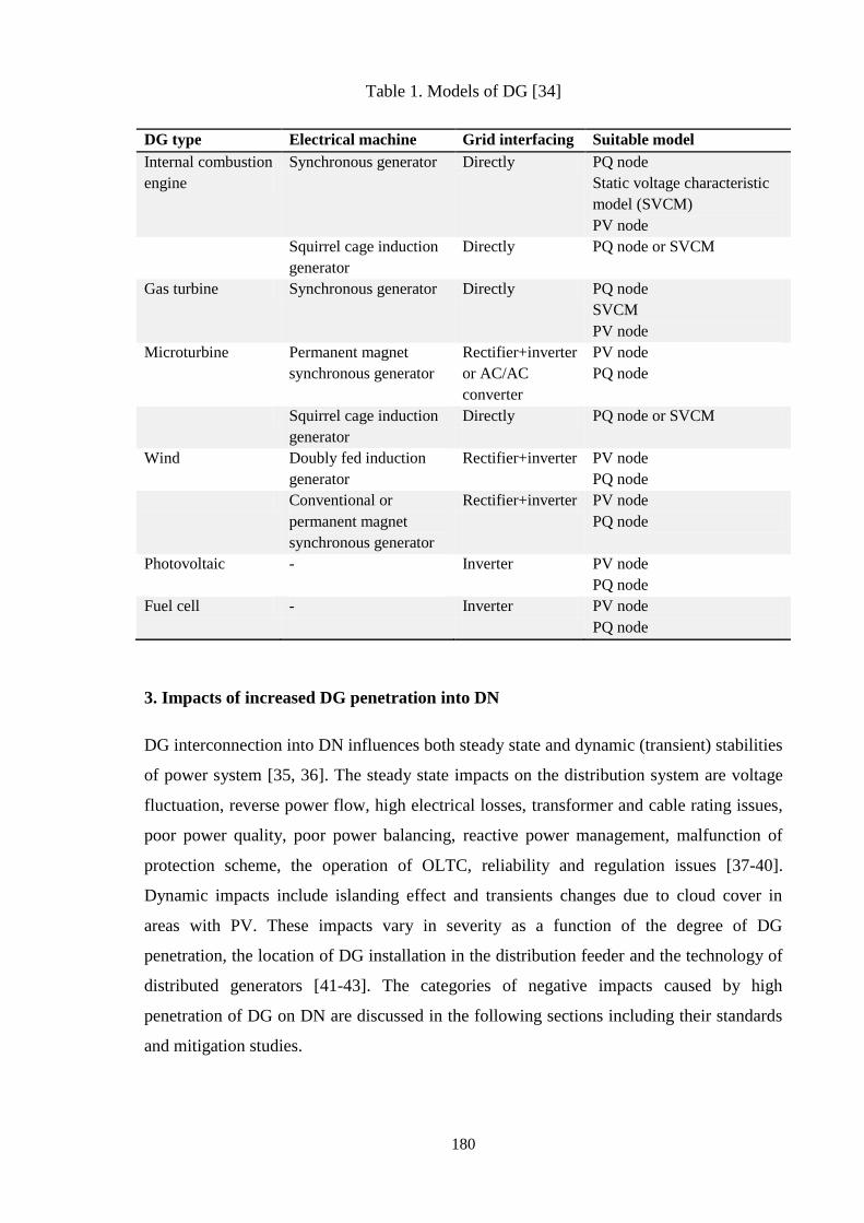
180

Table 1. Models of DG [34]

DG type Electrical machine Grid interfacing Suitable model

Internal combustion

engine

Synchronous generator Directly PQ node

Static voltage characteristic

model (SVCM)

PV node

Squirrel cage induction

generator

Directly PQ node or SVCM

Gas turbine Synchronous generator Directly PQ node

SVCM

PV node

Microturbine Permanent magnet

synchronous generator

Rectifier+inverter

or AC/AC

converter

PV node

PQ node

Squirrel cage induction

generator

Directly PQ node or SVCM

Wind Doubly fed induction

generator

Rectifier+inverter PV node

PQ node

Conventional or

permanent magnet

synchronous generator

Rectifier+inverter PV node

PQ node

Photovoltaic - Inverter PV node

PQ node

Fuel cell - Inverter PV node

PQ node

3. Impacts of increased DG penetration into DN

DG interconnection into DN influences both steady state and dynamic (transient) stabilities

of power system [35, 36]. The steady state impacts on the distribution system are voltage

fluctuation, reverse power flow, high electrical losses, transformer and cable rating issues,

poor power quality, poor power balancing, reactive power management, malfunction of

protection scheme, the operation of OLTC, reliability and regulation issues [37-40].

Dynamic impacts include islanding effect and transients changes due to cloud cover in

areas with PV. These impacts vary in severity as a function of the degree of DG

penetration, the location of DG installation in the distribution feeder and the technology of

distributed generators [41-43]. The categories of negative impacts caused by high

penetration of DG on DN are discussed in the following sections including their standards

and mitigation studies.

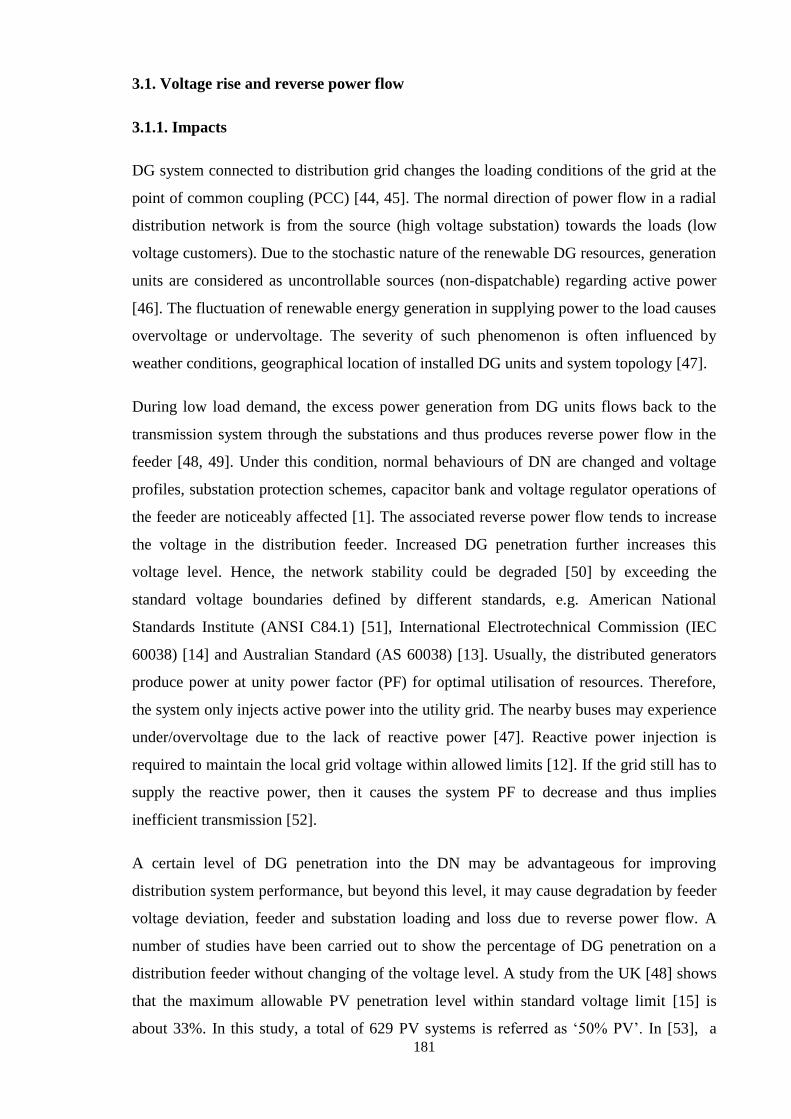
181

3.1. Voltage rise and reverse power flow

3.1.1. Impacts

DG system connected to distribution grid changes the loading conditions of the grid at the

point of common coupling (PCC) [44, 45]. The normal direction of power flow in a radial

distribution network is from the source (high voltage substation) towards the loads (low

voltage customers). Due to the stochastic nature of the renewable DG resources, generation

units are considered as uncontrollable sources (non-dispatchable) regarding active power

[46]. The fluctuation of renewable energy generation in supplying power to the load causes

overvoltage or undervoltage. The severity of such phenomenon is often influenced by

weather conditions, geographical location of installed DG units and system topology [47].

During low load demand, the excess power generation from DG units flows back to the

transmission system through the substations and thus produces reverse power flow in the

feeder [48, 49]. Under this condition, normal behaviours of DN are changed and voltage

profiles, substation protection schemes, capacitor bank and voltage regulator operations of

the feeder are noticeably affected [1]. The associated reverse power flow tends to increase

the voltage in the distribution feeder. Increased DG penetration further increases this

voltage level. Hence, the network stability could be degraded [50] by exceeding the

standard voltage boundaries defined by different standards, e.g. American National

Standards Institute (ANSI C84.1) [51], International Electrotechnical Commission (IEC

60038) [14] and Australian Standard (AS 60038) [13]. Usually, the distributed generators

produce power at unity power factor (PF) for optimal utilisation of resources. Therefore,

the system only injects active power into the utility grid. The nearby buses may experience

under/overvoltage due to the lack of reactive power [47]. Reactive power injection is

required to maintain the local grid voltage within allowed limits [12]. If the grid still has to

supply the reactive power, then it causes the system PF to decrease and thus implies

inefficient transmission [52].

A certain level of DG penetration into the DN may be advantageous for improving

distribution system performance, but beyond this level, it may cause degradation by feeder

voltage deviation, feeder and substation loading and loss due to reverse power flow. A

number of studies have been carried out to show the percentage of DG penetration on a

distribution feeder without changing of the voltage level. A study from the UK [48] shows

that the maximum allowable PV penetration level within standard voltage limit [15] is

about 33%. In this study, a total of 629 PV systems is referred as ‘50% PV’. In [53], a

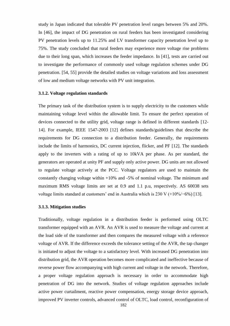
182

study in Japan indicated that tolerable PV penetration level ranges between 5% and 20%.

In [46], the impact of DG penetration on rural feeders has been investigated considering

PV penetration levels up to 11.25% and LV transformer capacity penetration level up to

75%. The study concluded that rural feeders may experience more voltage rise problems

due to their long span, which increases the feeder impedance. In [41], tests are carried out

to investigate the performance of commonly used voltage regulation schemes under DG

penetration. [54, 55] provide the detailed studies on voltage variations and loss assessment

of low and medium voltage networks with PV unit integration.

3.1.2. Voltage regulation standards

The primary task of the distribution system is to supply electricity to the customers while

maintaining voltage level within the allowable limit. To ensure the perfect operation of

devices connected to the utility grid, voltage range is defined in different standards [12-

14]. For example, IEEE 1547-2003 [12] defines standards/guidelines that describe the

requirements for DG connection to a distribution feeder. Generally, the requirements

include the limits of harmonics, DC current injection, flicker, and PF [12]. The standards

apply to the inverters with a rating of up to 10kVA per phase. As per standard, the

generators are operated at unity PF and supply only active power. DG units are not allowed

to regulate voltage actively at the PCC. Voltage regulators are used to maintain the

constantly changing voltage within +10% and -5% of nominal voltage. The minimum and

maximum RMS voltage limits are set at 0.9 and 1.1 p.u, respectively. AS 60038 sets

voltage limits standard at customers’ end in Australia which is 230 V (+10%/−6%) [13].

3.1.3. Mitigation studies

Traditionally, voltage regulation in a distribution feeder is performed using OLTC

transformer equipped with an AVR. An AVR is used to measure the voltage and current at

the load side of the transformer and then compares the measured voltage with a reference

voltage of AVR. If the difference exceeds the tolerance setting of the AVR, the tap changer

is initiated to adjust the voltage to a satisfactory level. With increased DG penetration into

distribution grid, the AVR operation becomes more complicated and ineffective because of

reverse power flow accompanying with high current and voltage in the network. Therefore,

a proper voltage regulation approach is necessary in order to accommodate high

penetration of DG into the network. Studies of voltage regulation approaches include

active power curtailment, reactive power compensation, energy storage device approach,

improved PV inverter controls, advanced control of OLTC, load control, reconfiguration of

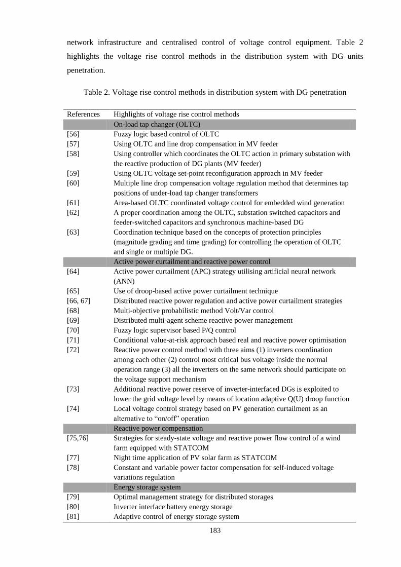
183

network infrastructure and centralised control of voltage control equipment. Table 2

highlights the voltage rise control methods in the distribution system with DG units

penetration.

Table 2. Voltage rise control methods in distribution system with DG penetration

References Highlights of voltage rise control methods

On-load tap changer (OLTC)

[56] Fuzzy logic based control of OLTC

[57] Using OLTC and line drop compensation in MV feeder

[58] Using controller which coordinates the OLTC action in primary substation with

the reactive production of DG plants (MV feeder)

[59] Using OLTC voltage set-point reconfiguration approach in MV feeder

[60] Multiple line drop compensation voltage regulation method that determines tap

positions of under-load tap changer transformers

[61] Area-based OLTC coordinated voltage control for embedded wind generation

[62] A proper coordination among the OLTC, substation switched capacitors and

feeder-switched capacitors and synchronous machine-based DG

[63] Coordination technique based on the concepts of protection principles

(magnitude grading and time grading) for controlling the operation of OLTC

and single or multiple DG.

Active power curtailment and reactive power control

[64] Active power curtailment (APC) strategy utilising artificial neural network

(ANN)

[65] Use of droop-based active power curtailment technique

[66, 67] Distributed reactive power regulation and active power curtailment strategies

[68] Multi-objective probabilistic method Volt/Var control

[69] Distributed multi-agent scheme reactive power management

[70] Fuzzy logic supervisor based P/Q control

[71] Conditional value-at-risk approach based real and reactive power optimisation

[72] Reactive power control method with three aims (1) inverters coordination

among each other (2) control most critical bus voltage inside the normal

operation range (3) all the inverters on the same network should participate on

the voltage support mechanism

[73] Additional reactive power reserve of inverter-interfaced DGs is exploited to

lower the grid voltage level by means of location adaptive Q(U) droop function

[74] Local voltage control strategy based on PV generation curtailment as an

alternative to “on/off” operation

Reactive power compensation

[75,76] Strategies for steady-state voltage and reactive power flow control of a wind

farm equipped with STATCOM

[77] Night time application of PV solar farm as STATCOM

[78] Constant and variable power factor compensation for self-induced voltage

variations regulation

Energy storage system

[79] Optimal management strategy for distributed storages

[80] Inverter interface battery energy storage

[81] Adaptive control of energy storage system

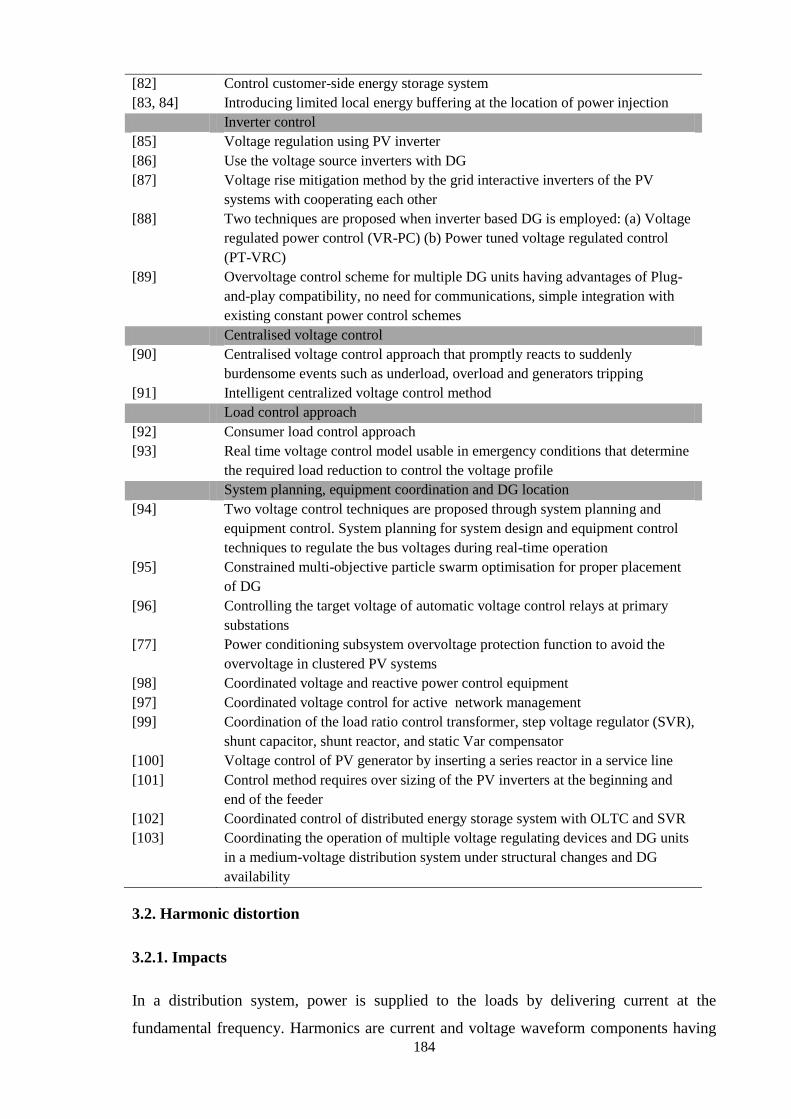
184

[82] Control customer-side energy storage system

[83, 84] Introducing limited local energy buffering at the location of power injection

Inverter control

[85] Voltage regulation using PV inverter

[86] Use the voltage source inverters with DG

[87] Voltage rise mitigation method by the grid interactive inverters of the PV

systems with cooperating each other

[88] Two techniques are proposed when inverter based DG is employed: (a) Voltage

regulated power control (VR-PC) (b) Power tuned voltage regulated control

(PT-VRC)

[89] Overvoltage control scheme for multiple DG units having advantages of Plug-

and-play compatibility, no need for communications, simple integration with

existing constant power control schemes

Centralised voltage control

[90] Centralised voltage control approach that promptly reacts to suddenly

burdensome events such as underload, overload and generators tripping

[91] Intelligent centralized voltage control method

Load control approach

[92] Consumer load control approach

[93] Real time voltage control model usable in emergency conditions that determine

the required load reduction to control the voltage profile

System planning, equipment coordination and DG location

[94] Two voltage control techniques are proposed through system planning and

equipment control. System planning for system design and equipment control

techniques to regulate the bus voltages during real-time operation

[95] Constrained multi-objective particle swarm optimisation for proper placement

of DG

[96] Controlling the target voltage of automatic voltage control relays at primary

substations

[77] Power conditioning subsystem overvoltage protection function to avoid the

overvoltage in clustered PV systems

[98] Coordinated voltage and reactive power control equipment

[97] Coordinated voltage control for active network management

[99] Coordination of the load ratio control transformer, step voltage regulator (SVR),

shunt capacitor, shunt reactor, and static Var compensator

[100] Voltage control of PV generator by inserting a series reactor in a service line

[101] Control method requires over sizing of the PV inverters at the beginning and

end of the feeder

[102] Coordinated control of distributed energy storage system with OLTC and SVR

[103] Coordinating the operation of multiple voltage regulating devices and DG units

in a medium-voltage distribution system under structural changes and DG

availability

3.2. Harmonic distortion

3.2.1. Impacts

In a distribution system, power is supplied to the loads by delivering current at the

fundamental frequency. Harmonics are current and voltage waveform components having

185

frequencies which are integral multiples of the fundamental frequency. On the other hand,

current and voltage components having frequencies which are not integral multiples of the

fundamental frequency are referred as interharmonics. Harmonic distortion in an electrical

system is the deviation of the voltage and current waveforms from a purely sinusoidal

waveform. In a distribution system with DG, power electronic converters/inverters are

used to convert the power from DG units to the correct voltage and frequency of the grid.

Harmonic distortion occurs when nonlinear loads draw non-sinusoidal current even

connected through a sinusoidal voltage source. This non-sinusoidal current contains

harmonic current that interacts with the impedance of distribution system and causes

voltage harmonics. The connection of a new converter unit can also be a reason of

increased total harmonic distortion (THD) at its PCC and in other buses. In a DG

interconnected system, harmonic distortions depend on the power converter technology.

Power electronics switching devices can inject high-frequency components rather than the

desired current.

With increased PVDG penetration in the power grid, harmonic resonance is becoming a

crucial issue in power systems [104]. In addition, PVDG placement also contributes to

harmonic distortion in a power system. DG placement at the higher voltage network

produces less harmonic distortion compared with a connection at the low voltage network

[105]. Harmonic resonance can occur at the PCC of an individual or multiple DG units to

the grid because of impedance mismatch between the grid and the inverter [106]. In a

distribution network with increased penetration of DG, pulse width modulation (PWM)

inverter harmonic currents can also be a cause of harmonic excitation for system resonance

[107]. Large scale penetration of DG into DN, fluorescent lights with high-frequency

ballast, computers equipped with active power-factor correction and adjustable-speed

drives are the reasons of distortion at frequencies above 1 or 2 kHz [108, 109].

Harmonic distortion causes numerous impacts on distribution system equipment and loads

connected to it. The impacts include high neutral currents, overheated main switchboards

components, phase conductors, transformers, random tripping of circuit breakers,

flickering lights, malfunction of sensitive equipment, fire hazards, reduced PF and system

efficiency due to excessive heating and reduction of equipment lifespan [110, 111]. The

effect of harmonic resonance presents severe power quality problems such as tripping of

protection devices and damaging of sensitive equipment because of overvoltage or

overcurrent [104].

186

The type and severity of harmonic problems depend on switching device technologies,

harmonics characteristics, equipment ratings, and loading conditions of the host

distribution feeder. This dependency decreases proportionally with reduced power

converter rating [112]. Increased level of DG penetration into distribution system can also

amplify harmonic distortion [113].

Several studies have been carried out regarding the maximum penetration level of DG unit

considering the IEEE Std. 519 harmonics limit [114]. In [105], the maximum DG

penetration level into DN for the centralised approach is determined considering harmonic

effect caused by inverter-based DG units. The results show that maximum penetration is

limited to 66.67% and 33.53% for 18 and 33 bus systems, respectively. In [115], the study

shows that the penetration level can reach to 100% of the feeder capacity considering IEEE

standard 519-1992 7th and 9th standard harmonic limits [114]. In [116], the effect of

harmonic distortion in a utility owned inverter-based DG system is considered to find the

maximum DG penetration level. The results found an optimal DG penetration level of

26.94% by placing DG units in an optimal location. In [117], the highest penetration of DG

with harmonics within the allowable range [114] was found 72% of the total capacity of

the transformer.

3.2.2. Standards

In the normal cases, studies on harmonic distortion are carried out considering frequency

range up to about 1 or 2 kHz [118], where the existing standards apply. For example, in

order to limit the harmonic injection in the network by the individual customers and the

utility, IEEE 519-1992 standard has set limits for harmonics [114]. For customers at 69kV

and below, harmonic voltage distortion limits are 3% on individual harmonic and 5% on

the THD. Table 3 presents the IEEE 519 harmonic current limit for general distribution

systems.

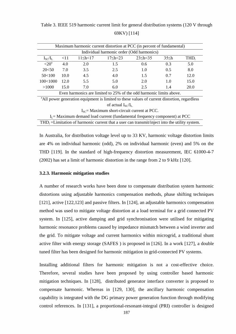
187

Table 3. IEEE 519 harmonic current limit for general distribution systems (120 V through

69KV) [114]

Maximum harmonic current distortion at PCC (in percent of fundamental)

Individual harmonic order (Odd harmonics)

ISC/IL <11 11≤h<17 17≤h<23 23≤h<35 35≤h THDi

<20a 4.0 2.0 1.5 0.6 0.3 5.0

20<50 7.0 3.5 2.5 1.0 0.5 8.0

50<100 10.0 4.5 4.0 1.5 0.7 12.0

100<1000 12.0 5.5 5.0 2.0 1.0 15.0

>1000 15.0 7.0 6.0 2.5 1.4 20.0

Even harmonics are limited to 25% of the odd harmonic limits above. aAll power generation equipment is limited to these values of current distortion, regardless

of actual ISC/IL.

ISC= Maximum short-circuit current at PCC.

IL= Maximum demand load current (fundamental frequency component) at PCC

THDi =Limitation of harmonic current that a user can transmit/inject into the utility system.

In Australia, for distribution voltage level up to 33 KV, harmonic voltage distortion limits

are 4% on individual harmonic (odd), 2% on individual harmonic (even) and 5% on the

THD [119]. In the standard of high-frequency distortion measurement, IEC 61000-4-7

(2002) has set a limit of harmonic distortion in the range from 2 to 9 kHz [120].

3.2.3. Harmonic mitigation studies

A number of research works have been done to compensate distribution system harmonic

distortions using adjustable harmonics compensation methods, phase shifting techniques

[121], active [122,123] and passive filters. In [124], an adjustable harmonics compensation

method was used to mitigate voltage distortion at a load terminal for a grid connected PV

system. In [125], active damping and grid synchronisation were utilised for mitigating

harmonic resonance problems caused by impedance mismatch between a wind inverter and

the grid. To mitigate voltage and current harmonics within microgrid, a traditional shunt

active filter with energy storage (SAFES ) is proposed in [126]. In a work [127], a double

tuned filter has been designed for harmonic mitigation in grid-connected PV systems.

Installing additional filters for harmonic mitigation is not a cost-effective choice.

Therefore, several studies have been proposed by using controller based harmonic

mitigation techniques. In [128], distributed generator interface converter is proposed to

compensate harmonic. Whereas in [129, 130], the ancillary harmonic compensation

capability is integrated with the DG primary power generation function through modifying

control references. In [131], a proportional-resonant-integral (PRI) controller is designed

188

for harmonic mitigation in a grid connected PV system. In [132], a double tuned PI-R

based current controller was used to mitigate grid side harmonic current in a DFIG based

wind power system. In [133], the virtual impedance method is suggested for harmonic

compensation based on converter control.

3.3. Voltage sag/dip

3.3.1. Impacts

According to IEEE Std. 1159-1995, voltage sag in the distribution system is a reduction of

RMS value of source voltage between 10 and 90 percent of nominal voltage for 10

milliseconds (ms) up to 60s (momentary interruption) [134]. Voltage sag could be

introduced from both internal and external sources. The sudden lightning strike is one of

the most common external causes. Internal causes include equipment failures, power line

contacts (line to a ground fault), short circuit fault, sudden load changing, transformer

energising (depending on transformer connection) and large motor start-ups (since starting

draw large current).

Voltage sag may cause apparatus tripping, shut down electrical equipment and destroy the

power electronic devices such as computers, industrial control systems, adjustable speed

drives, programmable logic controllers (PLC) and thus leads to economic losses. The

severity of voltage sag depends on the protection system design and coordination among

protective devices.

The integration of DG affects the performance of the protection scheme of distribution

system due to reverse power flow and therefore, the nature of voltage sags can be affected

by increased DG penetration [135]. Faults in the power system cause voltage dip at the

PCC. In a wind system, voltage dip may lead to the destruction of the converter by

increasing the current in the stator windings of the WT. Voltage dips that lead to increase

of currents can also occur when PMSG is connected to the grid via IGBT power electronic

inverters. A study revealed that DG may have a positive impact on the voltage sag

performance if the fault duration is no longer than 2s [135].

3.3.2. Voltage sag mitigations

Generally, voltage sag can be considerably mitigated by controlling the injected reactive

power at the PCC. Reactive power could be injected using series-connected voltage source

189

converters such as DVR [136] and STATCOM [137]. Energy storage units in DVRs can

also supply the active power component needed during voltage sag mitigation [138].

The use of grid-interfaces of distributed generators is an interesting approach to mitigate

power quality issues, especially voltage dips [139]. Generally, DG units are connected to

the utility grid via a voltage source converter (DC to AC) which could be utilised for

voltage sag mitigation [140, 141]. During sustained utility outages, DG reduces voltage

sags and acts as an instant backup [142]. In [136], DVR and distribution static compensator

(DSTATCOM) are used for restoring the voltage at the wind farm terminals under fault

conditions. Likewise, various DG-based schemes have been proposed for voltage dip

mitigation including:

(a) application of converter-based DG, synchronous and asynchronous generators [143,

144];

(b) series and shunt compensation [145, 146];

(c) SAFES [126];

(d) DSTATCOM with DG [147, 148];

(e) fault decoupling device [149];

(f) optimal DG allocation and sizing [150] and

(g) DVR with artificial intelligence (AI) [151].

3.4. Voltage fluctuation/flicker

3.4.1. Impacts of voltage fluctuation

Voltage fluctuation is a systematic variation of the voltage envelope or a series of random

voltage changes. It can be characterised by the fluctuations of two indices: amplitude and

frequency. If the voltage fluctuation occurs with the frequency from 0.05 Hz to 42 Hz, then

it is known as flicker which causes the luminance of incandescent lamps to fluctuate [152].

Rapid fluctuation of the power output of generators, load changes and induction motor

starting are the potential reasons of voltage flicker. Moreover, flicker emission is also

affected by the changes of the various grid conditions such as short-circuit ratio, type of

loads, and grid impedance angle [152].

Voltage fluctuation is considered as a major power quality problem. It can affect motor

starting, speed and causes disturbances to the applications driven by the affected motors

which can lead to equipment temperature rise and motor overloading. Therefore, it affects

190

the production, machine service life and thus increases economic losses. In diode rectifiers,

PF may be lowered and the harmonic currents will increase [152]. Also, it may reduce the

service lifetime of the electronic, incandescent, fluorescent and CRT devices [153]. Flicker

affects humans by causing light fluctuations that are irritating to the eyes.

In PV-DG system, voltage fluctuation occurs due to the stochastic nature of PV output.

Moreover, switching of PV inverters, poorly designed MPPT systems are the reasons of

unacceptable flicker emissions. DG units connected to weak supply networks can also

cause flicker in the distribution system [154].

In grid-connected wind energy system, wind shear and tower shadow are sources of power

fluctuation caused by wind speed variations. Voltage fluctuation depends on the

penetration level of DG into the distribution grid. High penetration of DG will also

increase the fluctuation [155]. Therefore, voltage fluctuation limits the penetration of DG

unit into DN.

3.4.2. Voltage fluctuation due to cloud passages

The sudden change of cloud condition is another reason for flicker emission [156] in PV-

DG system. In a study, the authors measure the rate of sunlight change caused by cloud

passages is from 60 to 150 W/m2/s is [157]. Spatial distribution significantly reduces the

transients caused by clouds [158]. During cloudy and foggy days, in a distribution system

with increased penetration of PV units, cloud passages induce undesirable voltage

fluctuations due to power generation fluctuations. This may lead to excessive operations of

the OLTC and creates flicker [158-160]. Balancing of power and fast ramping are two

ways to mitigate the effect of cloud passages and morning fog and to increase the overall

system reliability and efficiency. PV power generation needs to be balanced with other

very fast controllable sources such as gas, coal, other renewable energy sources or energy

storage systems [161].

Several studies have been carried out to determine the maximum penetration levels of DG

units into DN during cloud transients. Fast ramping using conventional generators could be

a way to lessen the effect of cloud transients where PV is deployed as a central generation

station. In a study [162], maximum tolerable PV penetration reached to 13.27%, where PV

was used as a central generation station. In another study [163], it was found that PV

penetration is limited to only 1.3% with ramping using coal-fired units installed at the

same central station. However, due to the smoothing effect of geographic diversity, the

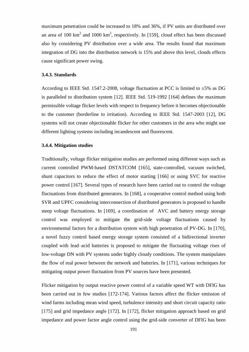
191

maximum penetration could be increased to 18% and 36%, if PV units are distributed over

an area of 100 km2 and 1000 km

2, respectively. In [159], cloud effect has been discussed

also by considering PV distribution over a wide area. The results found that maximum

integration of DG into the distribution network is 15% and above this level, clouds effects

cause significant power swing.

3.4.3. Standards

According to IEEE Std. 1547.2-2008, voltage fluctuation at PCC is limited to ±5% as DG

is paralleled to distribution system [12]. IEEE Std. 519-1992 [164] defines the maximum

permissible voltage flicker levels with respect to frequency before it becomes objectionable

to the customer (borderline to irritation). According to IEEE Std. 1547-2003 [12], DG

systems will not create objectionable flicker for other customers in the area who might use

different lighting systems including incandescent and fluorescent.


Traditionally, voltage flicker mitigation studies are performed using different ways such as

current controlled PWM-based DSTATCOM [165], state-controlled, vacuum switched,

shunt capacitors to reduce the effect of motor starting [166] or using SVC for reactive

power control [167]. Several types of research have been carried out to control the voltage

fluctuations from distributed generators. In [168], a cooperative control method using both

SVR and UPFC considering interconnection of distributed generators is proposed to handle

steep voltage fluctuations. In [169], a coordination of AVC and battery energy storage

control was employed to mitigate the grid-side voltage fluctuations caused by

environmental factors for a distribution system with high penetration of PV-DG. In [170],

a novel fuzzy control based energy storage system consisted of a bidirectional inverter

coupled with lead–acid batteries is proposed to mitigate the fluctuating voltage rises of

low-voltage DN with PV systems under highly cloudy conditions. The system manipulates

the flow of real power between the network and batteries. In [171], various techniques for

mitigating output power fluctuation from PV sources have been presented.

Flicker mitigation by output reactive power control of a variable speed WT with DFIG has

been carried out in few studies [172-174]. Various factors affect the flicker emission of

wind farms including mean wind speed, turbulence intensity and short circuit capacity ratio

[175] and grid impedance angle [172]. In [172], flicker mitigation approach based on grid

impedance and power factor angle control using the grid-side converter of DFIG has been

192

proposed. In another study [173], a rotor-side converter based reactive power control

scheme has been presented for flicker reduction during variable wind speed. In [174], the

reactive power has been controlled using STATCOM to study flicker of grid-connected

WT with DFIG. In a study [152], the combination of active power smoothening and

reactive power compensation has been proposed to suppress flicker. In order to mitigate

wind power fluctuations, an active current control of DFIG based technique is proposed in

[176]. In [177], different flicker mitigation solutions have been investigated in distributed

wind power. The solutions are based on the bandwidth of wind farm voltage controller,

increased MV/HV transformer rating, using two parallel MV/HV transformers, series line

compensation and changing of the wind farm connection point. The results show that these

mitigation systems are less effective for a wind farm except changing of the wind farm

connection point.

3.5. Voltage unbalance

3.5.1. Impacts

In a three-phase electric system, unequal line voltage magnitudes are defined as voltage

unbalance [178]. Use of single-phase distributed generators and unbalanced phase loads in

the electric system cause voltage unbalance. In a PV-DG system, increased penetration of

residential rooftop PV into the grid with random installation across distribution system is

also a reason for increasing or decreasing the network imbalance index [179].

Voltage unbalance creates negative effects on the distribution system which cause

overheating of equipment such as induction motors, power electronic converters and

adjustable speed drives, and power and energy losses in the distribution grid. Additionally,

network problems such as the malfunction of relays and voltage regulators, and generation

of non-characteristic harmonics from power electronic loads could be introduced.

Therefore, maintaining a balanced voltage at the point of connection is necessary in order

to mitigate voltage unbalance [180].

3.5.2. Standards

According to IEEE/ANSI C84.1-1995 standard, maximum voltage unbalance in a three

phase distribution system is limited to 3% [51].

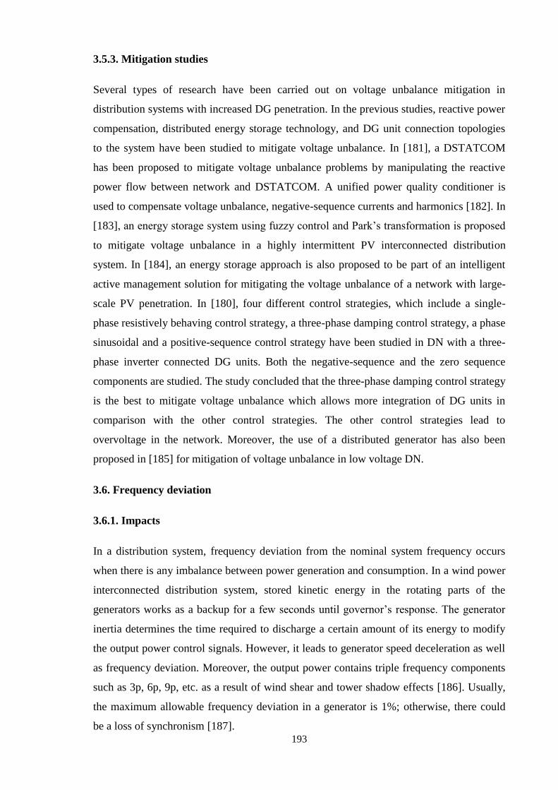
193


Several types of research have been carried out on voltage unbalance mitigation in

distribution systems with increased DG penetration. In the previous studies, reactive power

compensation, distributed energy storage technology, and DG unit connection topologies

to the system have been studied to mitigate voltage unbalance. In [181], a DSTATCOM

has been proposed to mitigate voltage unbalance problems by manipulating the reactive

power flow between network and DSTATCOM. A unified power quality conditioner is

used to compensate voltage unbalance, negative-sequence currents and harmonics [182]. In

[183], an energy storage system using fuzzy control and Park’s transformation is proposed

to mitigate voltage unbalance in a highly intermittent PV interconnected distribution

system. In [184], an energy storage approach is also proposed to be part of an intelligent

active management solution for mitigating the voltage unbalance of a network with large-

scale PV penetration. In [180], four different control strategies, which include a single-

phase resistively behaving control strategy, a three-phase damping control strategy, a phase

sinusoidal and a positive-sequence control strategy have been studied in DN with a three-

phase inverter connected DG units. Both the negative-sequence and the zero sequence

components are studied. The study concluded that the three-phase damping control strategy

is the best to mitigate voltage unbalance which allows more integration of DG units in

comparison with the other control strategies. The other control strategies lead to

overvoltage in the network. Moreover, the use of a distributed generator has also been

proposed in [185] for mitigation of voltage unbalance in low voltage DN.

3.6. Frequency deviation

3.6.1. Impacts

In a distribution system, frequency deviation from the nominal system frequency occurs

when there is any imbalance between power generation and consumption. In a wind power

interconnected distribution system, stored kinetic energy in the rotating parts of the

generators works as a backup for a few seconds until governor’s response. The generator

inertia determines the time required to discharge a certain amount of its energy to modify

the output power control signals. However, it leads to generator speed deceleration as well

as frequency deviation. Moreover, the output power contains triple frequency components

such as 3p, 6p, 9p, etc. as a result of wind shear and tower shadow effects [186]. Usually,

the maximum allowable frequency deviation in a generator is 1%; otherwise, there could

be a loss of synchronism [187].

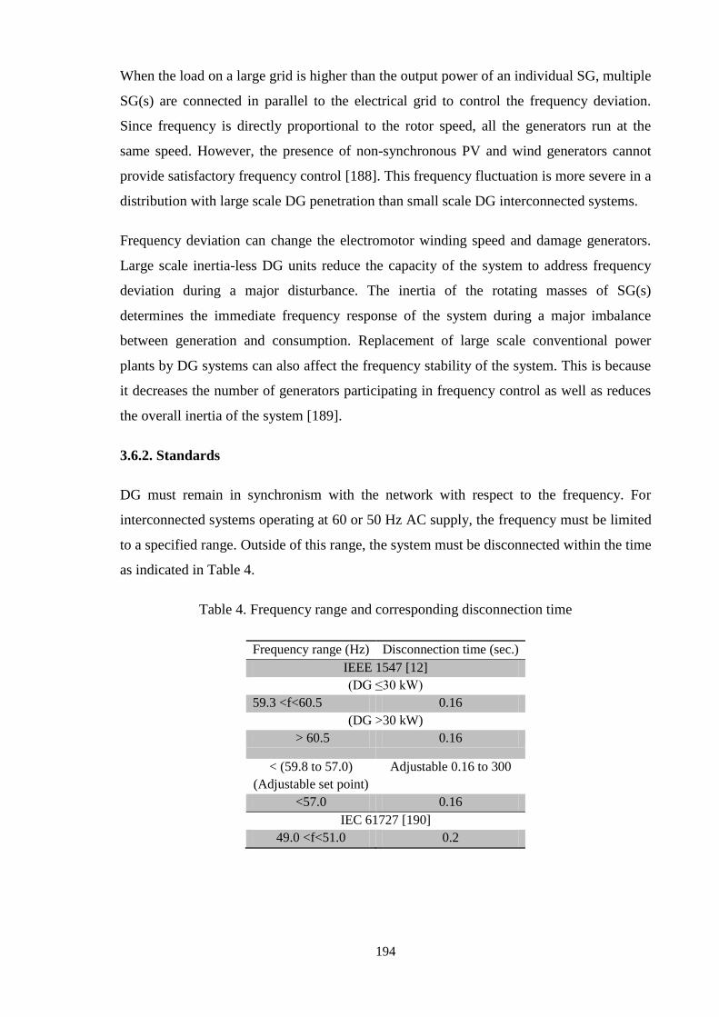
194

When the load on a large grid is higher than the output power of an individual SG, multiple

SG(s) are connected in parallel to the electrical grid to control the frequency deviation.

Since frequency is directly proportional to the rotor speed, all the generators run at the

same speed. However, the presence of non-synchronous PV and wind generators cannot

provide satisfactory frequency control [188]. This frequency fluctuation is more severe in a

distribution with large scale DG penetration than small scale DG interconnected systems.

Frequency deviation can change the electromotor winding speed and damage generators.

Large scale inertia-less DG units reduce the capacity of the system to address frequency

deviation during a major disturbance. The inertia of the rotating masses of SG(s)

determines the immediate frequency response of the system during a major imbalance

between generation and consumption. Replacement of large scale conventional power

plants by DG systems can also affect the frequency stability of the system. This is because

it decreases the number of generators participating in frequency control as well as reduces

the overall inertia of the system [189].

3.6.2. Standards

DG must remain in synchronism with the network with respect to the frequency. For

interconnected systems operating at 60 or 50 Hz AC supply, the frequency must be limited

to a specified range. Outside of this range, the system must be disconnected within the time

as indicated in Table 4.

Table 4. Frequency range and corresponding disconnection time

Frequency range (Hz) Disconnection time (sec.)

IEEE 1547 [12]

(DG ≤30 kW)

59.3 <f<60.5 0.16

(DG >30 kW)

> 60.5 0.16

< (59.8 to 57.0)

(Adjustable set point)

Adjustable 0.16 to 300

<57.0 0.16

IEC 61727 [190]

49.0 <f<51.0 0.2

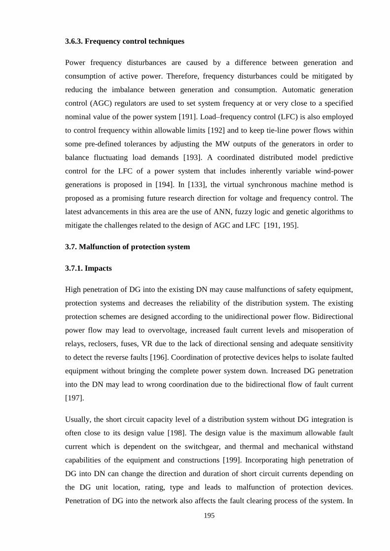
195

3.6.3. Frequency control techniques

Power frequency disturbances are caused by a difference between generation and

consumption of active power. Therefore, frequency disturbances could be mitigated by

reducing the imbalance between generation and consumption. Automatic generation

control (AGC) regulators are used to set system frequency at or very close to a specified

nominal value of the power system [191]. Load–frequency control (LFC) is also employed

to control frequency within allowable limits [192] and to keep tie-line power flows within

some pre-defined tolerances by adjusting the MW outputs of the generators in order to

balance fluctuating load demands [193]. A coordinated distributed model predictive

control for the LFC of a power system that includes inherently variable wind-power

generations is proposed in [194]. In [133], the virtual synchronous machine method is

proposed as a promising future research direction for voltage and frequency control. The

latest advancements in this area are the use of ANN, fuzzy logic and genetic algorithms to

mitigate the challenges related to the design of AGC and LFC [191, 195].

3.7. Malfunction of protection system

3.7.1. Impacts

High penetration of DG into the existing DN may cause malfunctions of safety equipment,

protection systems and decreases the reliability of the distribution system. The existing

protection schemes are designed according to the unidirectional power flow. Bidirectional

power flow may lead to overvoltage, increased fault current levels and misoperation of

relays, reclosers, fuses, VR due to the lack of directional sensing and adequate sensitivity

to detect the reverse faults [196]. Coordination of protective devices helps to isolate faulted

equipment without bringing the complete power system down. Increased DG penetration

into the DN may lead to wrong coordination due to the bidirectional flow of fault current

[197].

Usually, the short circuit capacity level of a distribution system without DG integration is

often close to its design value [198]. The design value is the maximum allowable fault

current which is dependent on the switchgear, and thermal and mechanical withstand

capabilities of the equipment and constructions [199]. Incorporating high penetration of

DG into DN can change the direction and duration of short circuit currents depending on

the DG unit location, rating, type and leads to malfunction of protection devices.

Penetration of DG into the network also affects the fault clearing process of the system. In

196

a radial distribution system, there is only one power source and the opening of only one

protective device acts for fault clearance. A combination of automatic recloser devices,

circuit breakers, sectionalizers, and fuses is applied to clear the temporary single-phase to

ground faults (about 80% of the network faults) and isolates the faulty part from the rest of

the system [200]. Large scale integration of DG units contains multiple power sources

which contribute to fault currents and the opening of only one protective device does not

guarantee the fast clearance of the fault. This interrupts the operation of the conventional

auto reclosing system and prevents temporary faults from being cleared. Therefore, it may

damage the distributed SG(s) due to an out of phase reclosing during power restoration

process. In order to maintain normal fault clearing processes, it is a requirement to

disconnect DG from the system when a fault is suspected before the elapsed time of fast

reclosing.

If a utility grid gets isolated, islanded operation occurs when only DG unit supplies power

to the local loads. This can happen due to some emergency conditions associated with

system safety, equipment protection and system control. The islanded could happen

through intentionally (planned operation) or unintentionally (unplanned operation).

Unintentional islanding may cause a hazardous effect on devices and to the public when a

portion of DN becomes electrically isolated from the system but still, continues to be

energised by the DG connection to the isolated subsystem. The main hazards and risks

associated with the unintentional islanding are discussed as follows [201]:

- Exceeding the acceptable limits of power quality parameters which can lead to the failure

of network and customer equipment;

- Uncleared faults (earth or phase faults) due to low short-circuit capacity or unearthed

operation. Can cause possible damage to the network components, otherwise sustain the

fault currents;

- Out of phase reclosing of protection device may damage protection equipment and causes

high transient inrush currents which may lead to the failure of generator;

- Electric shock.

197

3.7.2. Necessary standards for protection

3.7.2.1. Reconnection

The reconnection of one or more generators particularly after an outage or fault needs a

time delay after the system steady-state voltage and frequency are restored to the standard

ranges [12]. IEEE Std. 1547 recommends that it requires at least 5 minutes of normal

operation for a generator before reconnection [12].

3.7.2.2. Islanding detection

According to IEEE Std. 1547-2003, the unintentional island should be detected and

isolated within 2 s [12].

3.7.3. Protection systems

3.7.3.1. Protection system for islanding detection

The effective detection of unintentional islanding is essential for avoiding unwanted

hazardous effects. Remote and local detection techniques, signal processing and intelligent

classifiers are utilised to detect islanding in the distribution system. Remote techniques

require a communication scheme. These techniques are based on supervisory control and

data acquisition (SCADA) system, transfer trip scheme and inter-tripping. Local

techniques are developed based on local information and classified into active, passive and

hybrid techniques. Impedance measurement and slip mode frequency shift are popular

active methods. Passive techniques include under/over voltage monitoring, under/over

frequency monitoring, voltage phase jump detection and harmonic measurement. A hybrid

system is the combination of active and passive techniques. These techniques are: voltage

unbalance and frequency set point reconfiguration approach [202], voltage and real power

shift, voltage fluctuation injection and hybrid SFS and Q–f islanding technique [203, 204].

Wavelet-transform and S-transform are signal processing methods used for identification

of island mode operation. Common AI classifiers used in islanding detection include the

decision tree, rule-based techniques, ANN, probabilistic neural network, fuzzy logic, and

support vector machines.

3.7.3.2. Protection coordination methods

Several studies have been carried out to solve the overcurrent relay coordination problem

in distribution systems with increased penetration of DG units. These can be divided into

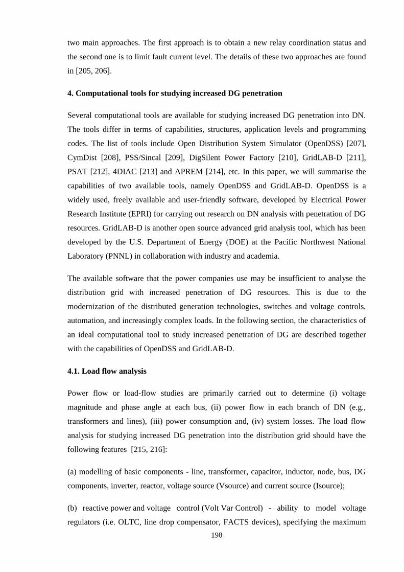
198

two main approaches. The first approach is to obtain a new relay coordination status and

the second one is to limit fault current level. The details of these two approaches are found

in [205, 206].

4. Computational tools for studying increased DG penetration

Several computational tools are available for studying increased DG penetration into DN.

The tools differ in terms of capabilities, structures, application levels and programming

codes. The list of tools include Open Distribution System Simulator (OpenDSS) [207],

CymDist [208], PSS/Sincal [209], DigSilent Power Factory [210], GridLAB-D [211],

PSAT [212], 4DIAC [213] and APREM [214], etc. In this paper, we will summarise the

capabilities of two available tools, namely OpenDSS and GridLAB-D. OpenDSS is a

widely used, freely available and user-friendly software, developed by Electrical Power

Research Institute (EPRI) for carrying out research on DN analysis with penetration of DG

resources. GridLAB-D is another open source advanced grid analysis tool, which has been

developed by the U.S. Department of Energy (DOE) at the Pacific Northwest National

Laboratory (PNNL) in collaboration with industry and academia.

The available software that the power companies use may be insufficient to analyse the

distribution grid with increased penetration of DG resources. This is due to the

modernization of the distributed generation technologies, switches and voltage controls,

automation, and increasingly complex loads. In the following section, the characteristics of

an ideal computational tool to study increased penetration of DG are described together

with the capabilities of OpenDSS and GridLAB-D.

4.1. Load flow analysis

Power flow or load-flow studies are primarily carried out to determine (i) voltage

magnitude and phase angle at each bus, (ii) power flow in each branch of DN (e.g.,

transformers and lines), (iii) power consumption and, (iv) system losses. The load flow

analysis for studying increased DG penetration into the distribution grid should have the

following features [215, 216]:

(a) modelling of basic components - line, transformer, capacitor, inductor, node, bus, DG

components, inverter, reactor, voltage source (Vsource) and current source (Isource);

(b) reactive power and voltage control (Volt Var Control) - ability to model voltage

regulators (i.e. OLTC, line drop compensator, FACTS devices), specifying the maximum

199

and minimum voltage limit, the tolerance on regulation settings; switching capacitor based

on both time and electrical quantities (voltage, current, kVAr); also, options for automatic

switching and reconfiguration as well as new localized and generation-based voltage

regulation systems which have been discussed in Section 3.1.3 to study increased DG

penetration into DN rather than usual voltage regulators;

(c) load flow modelling - for both balanced or unbalanced systems, single-phase/three-

phase load flow;

(d) time series simulation - most distribution system analysis tools are commonly designed

to study peak and off-peak loadings rather than different time-dependent loads based on

LDC. Computational tool must handle hourly/daily/weekly/annual/seasonal loads,

generation profiles and interruption rates to analyse the range of load demand and

generation which depends on times;

(e) sensitivity studies - for losses, voltage profile, feeder reconfiguration and capacitor

placement/size;

(f) modelling single or multiple distributed generators at the same load location of

distribution network;

(g) automatically retrieve of environmental and weather data (e.g. solar irradiance, wind

speed).

4.1.1. OpenDSS capabilities

OpenDSS includes a large number of circuit components to perform distribution system

analysis with integration of DG systems. The circuit components are divided into four

classes which are power delivery (PD), power conversion (PC), control and protection, and

meter elements. The PD components are line, transformer, capacitor, and reactor. The PC

components are load, generator, Vsource, Isource, PV system and storage. A total of six

control elements can be modelled using OpenDSS which include capacitor control, voltage

regulator, generator dispatcher, switch controller, storage controller and inverter controller.

Energy meters, monitors and sensors are three-meter elements implemented in this

software. The software can model n-phase, m-winding transformers rather than traditional

two or three winding models. In OpenDSS, seven types of loads can be modelled: (a)

conventional constant P, Q load model (b) constant Z load model (P and Q vary by the

square of the voltage) (c) constant P but Q is modelled as a constant reactance (d) P and Q

200

variation defined by exponential models (e) constant current magnitude which is common

in distribution system analysis (P and Q vary linearly with voltage magnitude) (f) constant

P that can be modified by load shape multipliers, but Q is a fixed value independent of

time (g) similar to (f), but Q is computed from a fixed reactance (varies with square of

voltage).

OpenDSS enables sequential time simulations called ‘quasi-static solutions’. This feature

makes OpenDSS suitable to study DG integration with DN since the availability of some

DG resources varies with time. A few examples of time-varying models are: (a) electric

vehicle charging (minutes, hours) (b) solar and wind generation (seconds) (c) dispatchable

generation (minutes to hours) (d) storage (minutes to hours) (e) energy efficiency (hours)

(f) distribution state estimation (seconds, minutes) (g) customers' load models (minutes to

hours) ( h) end-use thermal models (minutes to hours).

OpenDSS includes a lot of calculation modes for power flow studies including [207]

(a) Snapshot mode - This is a single snapshot power flow calculation mode in an iterative

method. The global load multiplier (LoadMult) and the growth factor for the present

year (Year) are used to modify the loads.

(b) Direct mode - This mode is also a single snapshot power flow studies mode that uses

an admittance model of all loads. This is non-iterative and just a direct method using

the currently specified voltage and current sources.

(c) Daily mode - The daily mode evaluates a series of power flow calculation following

the daily load curves. The peak load is determined by the ‘LoadMult’ and the growth

factor for the present year.

(d) Yearly mode - The yearly mode enables a series of power flow calculation following

the yearly load curves.

(e) Peak day mode - It performs the power flow studies only for those days, where the

peak exceeds a specified value.

(f) Duty cycle mode - The mode solves the power flow calculation following the duty

cycle curves with the time increment specified.

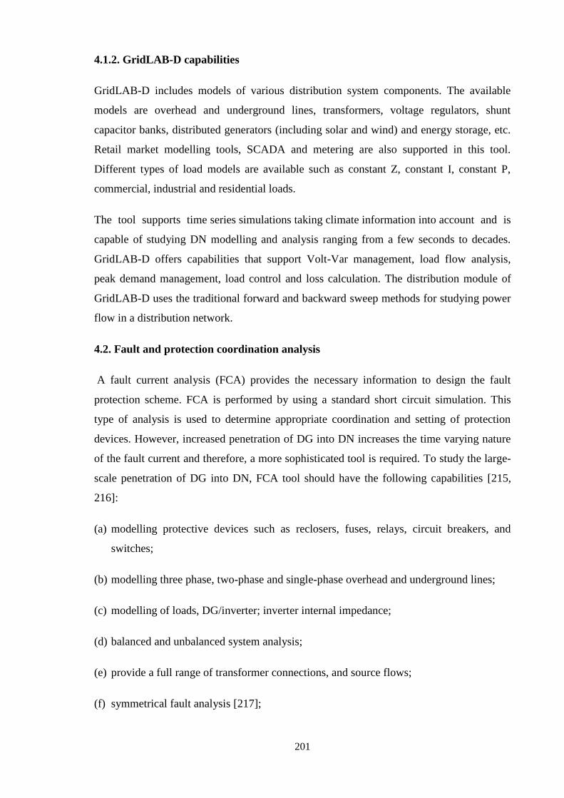
201

4.1.2. GridLAB-D capabilities

GridLAB-D includes models of various distribution system components. The available

models are overhead and underground lines, transformers, voltage regulators, shunt

capacitor banks, distributed generators (including solar and wind) and energy storage, etc.

Retail market modelling tools, SCADA and metering are also supported in this tool.

Different types of load models are available such as constant Z, constant I, constant P,

commercial, industrial and residential loads.

The tool supports time series simulations taking climate information into account and is

capable of studying DN modelling and analysis ranging from a few seconds to decades.

GridLAB-D offers capabilities that support Volt-Var management, load flow analysis,

peak demand management, load control and loss calculation. The distribution module of

GridLAB-D uses the traditional forward and backward sweep methods for studying power

flow in a distribution network.

4.2. Fault and protection coordination analysis

A fault current analysis (FCA) provides the necessary information to design the fault

protection scheme. FCA is performed by using a standard short circuit simulation. This

type of analysis is used to determine appropriate coordination and setting of protection

devices. However, increased penetration of DG into DN increases the time varying nature

of the fault current and therefore, a more sophisticated tool is required. To study the large-

scale penetration of DG into DN, FCA tool should have the following capabilities [215,

216]:

(a) modelling protective devices such as reclosers, fuses, relays, circuit breakers, and

switches;

(b) modelling three phase, two-phase and single-phase overhead and underground lines;

(c) modelling of loads, DG/inverter; inverter internal impedance;

(d) balanced and unbalanced system analysis;

(e) provide a full range of transformer connections, and source flows;

(f) symmetrical fault analysis [217];

202

(g) asymmetrical fault analysis (single line to ground, double line to ground and line to line

faults);

(h) modelling fault resistance;

(i) analysis fault current flow under different switching [218];

(j) identify and determine overvoltage during faults;

(k) protection device coordination analysis;

(l) interfacing capability with protection and reliability analysis software.

Generally, radial distribution network is protected by time overcurrent relays, circuit

breakers, reclosers, fuses, and sectionalizers. Protection coordination among these devices

is achieved through variable time delays in each protective device, where downstream

devices operate faster than upstream devices at any specific current. The contribution of

fault current from the DG must be quantified and considered in combination with load

characteristics. Protection coordination needs to be recoordinated or redesigned in this

situation. Moreover, software tools need to recognise the following two effects where

protective approach may fail or may be degraded [215]: (a) where SG(s) and some

inverters supply fault current which may cause malfunction of the time overcurrent

protection system and (b) in intentionally islanded systems, where fault current is low and

varies widely.

Both OpenDSS and GridLAB-D could be used for protection system simulation. In

OpenDSS, fault study mode can implement FCA in DG connected distribution system.

GridLAB-D also includes the studies of fault detection, device coordination, automation

and feeder reconfiguration. Table 5 presents a comparison of fault and protection

coordination analysis capabilities of these two tools.

203

Table 5. Fault and protection coordination analysis capabilities of OpenDSS and GridLAB-

D

Type of study OpenDSS GridLAB-D

Modelling recloser, fuse, relay, circuit breaker, and switches Yes Yes

Modelling three phase, two phase and single phase lines Yes Yes

Modelling of three phase, two phase and single phase loads Yes Yes

Balanced and unbalanced system analysis Yes Yes

Single-phase or three-phase transformer configurations Yes Yes

Modelling of DGs Yes Yes

Investigation of symmetrical and unsymmetrical faults Yes Yes

Modelling fault resistance Yes -

Protection coordination - Yes

Fault analysis in DG connected distribution system Yes -

4.3. Dynamic analysis

Dynamic analysis investigates the system ability to maintain stability during faults and

small signal fault conditions. It is recommended for a distribution system with high

penetration of DG in order to maintain the system stability during voltage and frequency

oscillations and rotor angle swing of distributed generators.

OpenDSS can perform basic electromechanical transient simulations. The capability has

been expanding steadily due to needs in inverter modelling and other applications where

machine dynamics are important. The built‐in generator model has a simple single‐mass

model that is adequate for many DG studies for common distribution system fault

conditions. In GridLAB-B, there is a dynamic mode, but the support is very limited.

4.4. Power quality analysis

In a distribution system equipped with DG through power electronic converters, power

quality analysis tool must be able to cover the following areas [219]

(a) able to analyse impulsive and oscillatory transients [220];

(b) able to study high-frequency harmonic and interharmonic interferences;

(c) modelling three-phase as well as all phases harmonics independently for analysing

multiple single phase DG applications;

204

(d) able to analyse voltage fluctuation. In a distribution system integrated with multiple DG

systems, modelling of DG considering flicker could be a challenging task for some DG

units, where there is no enough correlation between amount of output power fluctuation

and distribution resource;

(e) able to analyse voltage sag with capabilities of short-circuit calculations;

(f) able to simulate temporary overvoltages due to phase-earth faults, load rejection,

Ferranti rise, resonance, ferroresonance phenomena and lightening (see Ref [218] for

details);

(g) calculation of power quality indices such as system average RMS variation frequency

index, THD, PF, voltage distortion index, unbalance factor, transformer derating factor,

and flicker factor [221, 222].

OpenDSS is a frequency domain tool which supports all RMS steady-state analyses (i.e.,

sinusoidal steady state, but not limited to fundamental frequency) [207]. This tool has been

used for harmonic and interharmonic distortion analysis. Harmonics mode can implement

harmonic analysis. In terms of harmonics analysis, OpenDSS is better than GridLAB-D.

OpenDSS software can analyse voltage sag with capabilities of short-circuit calculations.

Overvoltage study can also be carried out using this tool. In the case of short circuit

calculation, GridLAB-D does not support short circuit contribution of DG sources.

4.5. Reliability analysis

Reliability primarily relates to DN components' failure and repair rates. The results could

be used to evaluate the reliability indices of distribution system. The important features of

the reliability analysis software are [223]:

(a) full three phase representations with the large-scale interconnection of DG units during

various normal and abnormal conditions;

(b) integration of reliability tools with advanced metering systems and information for

characterising and forecasting load profiles;

(c) databases of equipment reliability. Due to severe time constraints, most users currently

use average or assumed typical values (failure rate, restoration time of system

components);

205

(d) able to calculate distribution reliability measures for sustained and momentary

interruptions;

(e) risk assessment approaches;

(f) economics of reliability evaluation;

(g) calculation of voltage sags and sustained interruptions as well as reliability indices such

as SAIFI, SAIFI;

(h) considering the uncertainty modelling of DG parameters [224, 225].

In OpenDSS, the application of Monte Carlo method can be implemented for distribution

system reliability analysis. The software can carry out risk‐based distribution planning

studies. The software should include reliability economics assessment methods.

GridLAB-D can assess the reliability of DN. The results include reliability indices and

business metrics such as profitability, revenue rates of return and per customer or per line

mile cost.

4.6. Object oriented, interfacing and co-simulation

The required tool should have the following co-simulation facilities:

(a) able to model new components and controls to support advanced analyses related to

smart grid, grid modernization, increased DG penetration and renewable energy

research;

(b) interfacing to other programming tools (e.g., MATLAB, Visual Basic) to facilitate

post-processing of the simulation results which offers required plotting and calculation

benefits;

(c) option for co-simulation with communication networks.

OpenDSS is an object oriented program and commands can be implemented both as

standalone EXE program and component object model (COM) dynamic-link library (DLL)

interface. DLLs can be written in most common programming languages such as

MATLAB, Python, C++, R and other languages. However, the lack of a visual interface is

the limitation of OpenDSS.

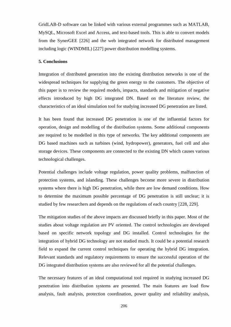
206

GridLAB‐D software can be linked with various external programmes such as MATLAB,

MySQL, Microsoft Excel and Access, and text-based tools. This is able to convert models

from the SynerGEE [226] and the web integrated network for distributed management

including logic (WINDMIL) [227] power distribution modelling systems.

5. Conclusions

Integration of distributed generation into the existing distribution networks is one of the

widespread techniques for supplying the green energy to the customers. The objective of

this paper is to review the required models, impacts, standards and mitigation of negative

effects introduced by high DG integrated DN. Based on the literature review, the

characteristics of an ideal simulation tool for studying increased DG penetration are listed.

It has been found that increased DG penetration is one of the influential factors for

operation, design and modelling of the distribution systems. Some additional components

are required to be modelled in this type of networks. The key additional components are

DG based machines such as turbines (wind, hydropower), generators, fuel cell and also

storage devices. These components are connected to the existing DN which causes various

technological challenges.

Potential challenges include voltage regulation, power quality problems, malfunction of

protection systems, and islanding. These challenges become more severe in distribution

systems where there is high DG penetration, while there are low demand conditions. How

to determine the maximum possible percentage of DG penetration is still unclear; it is

studied by few researchers and depends on the regulations of each country [228, 229].

The mitigation studies of the above impacts are discussed briefly in this paper. Most of the

studies about voltage regulation are PV oriented. The control technologies are developed

based on specific network topology and DG installed. Control technologies for the

integration of hybrid DG technology are not studied much. It could be a potential research

field to expand the current control techniques for operating the hybrid DG integration.

Relevant standards and regulatory requirements to ensure the successful operation of the

DG integrated distribution systems are also reviewed for all the potential challenges.

The necessary features of an ideal computational tool required in studying increased DG

penetration into distribution systems are presented. The main features are load flow

analysis, fault analysis, protection coordination, power quality and reliability analysis,

207

dynamic stability analysis. Also, the computational tool could have the facility to interface

with other programming tools. The comparison between two available tools has been

studied by their main features and limitations. Most of the available tools have various

specific features for particular topology and control techniques. But for an ideal tool, all

the required features including modelling of all types of DG into DN should have been

implemented in one platform. For reliability analysis, it is suggested that advanced Monte

Carlo methods [230] considering the uncertainty parameters of DG could be included to

reduce the computational complexity. It is expected that this review will be beneficial to

the users, designers, manufacturers, researchers of distribution systems for developing the

new computational tool by taking consideration of increased DG penetration.

References

[1] Ackermann T, Andersson G, Söder L. Distributed generation: a definition. Electr

Power Syst Res 2001;57(3):195-204.

[2] Bayod-Rújula AA. Future development of the electricity systems with distributed

generation. Energy 2009;34(3):377-83.

[3] Haque MM, Wolfs P. A review of high PV penetrations in LV distribution networks:

Present status, impacts and mitigation measures. Renew Sustain Energy Rev 2016;

62:1195-1208.

[4] Petinrin J, Shaabanb M. Impact of renewable generation on voltage control in

distribution systems. Renew Sustain Energy Rev 2016; 65:770-83.

[5] Marinopoulos AG, Alexiadis MC, Dokopoulos PS. Energy losses in a distribution line

with distributed generation based on stochastic power flow. Electr Power Syst Res

2011;81(10):1986-94.

[6] Kersting WH, Phillips WH. Distribution feeder line models. In: Proceedings of 38th

annual rural electric power conference;1994. p. A4/1-A4/8.

[7] Willis HL. Power distribution planning reference book: CRC press; 2004.

[8] Mota LTM, Mota AA. Load modeling at electric power distribution substations using

dynamic load parameters estimation. Int J Electr Power Energy Syst 2004;26(10):805-11.

[9] Roy N, Hossain M, Pota H. Effects of load modeling in power distribution system with

distributed wind generation. In: Proceedings of IEEE 21st Australasian universities power

engineering conference (AUPEC); 2011. p. 1-6.

208

[10] Concordia C, Ihara S. Load representation in power system stability studies. IEEE

Trans Power Appar Syst 1982:969-77.

[11] Al-Muhaini M, Heydt GT. Evaluating future power distribution system reliability

including distributed generation. IEEE Trans Power Delivery 2013;28(4):2264-72.

[12] IEEE standard for interconnecting distributed resources with electric power systems.

IEEE Std. 1547–2003:1-28.

[13] Standard voltages. Australian Std. 60038-2000.

[14] IEC standard voltages int electrotech comm. IEC 60038; 2002–07,6.2.

[15] BS EN 50160: Voltage characteristics of electricity supplied by public distribution

systems. British standards institution; 2000.

[16] Sarimuthu CR, Ramachandaramurthy VK, Agileswari K, Mokhlis H. A review on

voltage control methods using on-load tap changer transformers for networks with

renewable energy sources. Renew Sustain Energy Rev 2016;62:1154-61.

[17] Gao C, Redfern MA. A review of voltage control techniques of networks with

distributed generations using On-Load Tap Changer transformers. In: Proceedings of

IEEE 45th international universities power engineering conference (UPEC); 2010. p. 1-6.

[18] Y.-H. Song and A. Johns, Flexible ac transmission systems (FACTS): IET, 1999.

[19] Oomori T, Genji T, Yura T, Watanabe T, Takayama S, Fukuyama Y. Development of

equipment models for fast distribution three‐phase unbalanced load flow calculation. Electr

Eng Japan 2003;142(3):8-19.

[20] Sen KK. SSSC-static synchronous series compensator: theory, modeling, and

application. Power Delivery, IEEE Transactions on 1998;13(1):241-6.

[21] Ghosh A, Ledwich G. Compensation of distribution system voltage using DVR. IEEE

Trans Power Delivery 2002;17(4):1030-6.

[22] Mondal D, Chakrabarti A, Sengupta A. Power system small signal stability analysis

and control: Academic press; 2014.

[23] Gyugyi L. Power electronics in electric utilities: static var compensators. In:

Proceedings of the IEEE 1988;76(4):483-94.

[24] Rao P, Crow M, Yang Z. STATCOM control for power system voltage control

applications. IEEE Trans Power Delivery 2000;15(4):1311-7.

209

[25] Sen KK, Stacey EJ. UPFC-unified power flow controller: theory, modeling, and

applications. IEEE Trans Power Delivery 1998;13(4):1453-60.

[26] Mahmoud MS, AL-Sunni FM. Control and optimization of distributed generation

systems. Springer; 2015.

[27] Pilavachi P. Power generation with gas turbine systems and combined heat and power.

Appl Therm Eng 2000;20:1421-29.

[28] Saha A, Chowdhury S, Chowdhury S, Crossley P, Gaunt C. Microturbine based

distributed generator in smart grid application. In: Proceedings of IET 20th international

conference and exhibition on electricity distribution-part 1; 2009. p. 1-6.

[29] Azadani EN, Canizares C, Bhattacharya K. Modeling and stability analysis of

distributed generation. In: Proceedings of IEEE power and energy society general meeting;

2012. p. 1-8.

[30] Das V, Padmanaban S, Venkitusamy K, Selvamuthukumaran R, Blaabjerg F, Siano P.

Recent advances and challenges of fuel cell based power system architectures and control–

A review. Renew Sustain Energy Rev 2017;73:10-18.

[31] Jawahar C, Michael PA. A review on turbines for micro hydro power plant. Renew

Sustain Energy Rev 2017;72:882-7.

[32] Divya K, Rao PN. Models for wind turbine generating systems and their application in

load flow studies. Electr Power Syst Res 2006;76(9):844-56.

[33] Lopes J, Moreira C, Madureira A. Defining control strategies for microgrids islanded

operation. IEEE Trans Power Syst 2006;21(2):916-24.

[34] Moghaddas-Tafreshi S, Mashhour E. Distributed generation modeling for power flow

studies and a three-phase unbalanced power flow solution for radial distribution systems

considering distributed generation. Electr Power Syst Res 2009;79(4):680-6.

[35] Alam MJ, Muttaqi KM, Sutanto D, Elder L, Baitch A. Performance analysis of

distribution networks under high penetration of solar PV. In: Proceedings of 44th

international conference on large high voltage electric systems; 2012.

[36] Lopes JP, Hatziargyriou N, Mutale J, Djapic P, Jenkins N. Integrating distributed

generation into electric power systems: A review of drivers, challenges and opportunities.

Electr Power Syst Res 2007;77(9):1189-203.

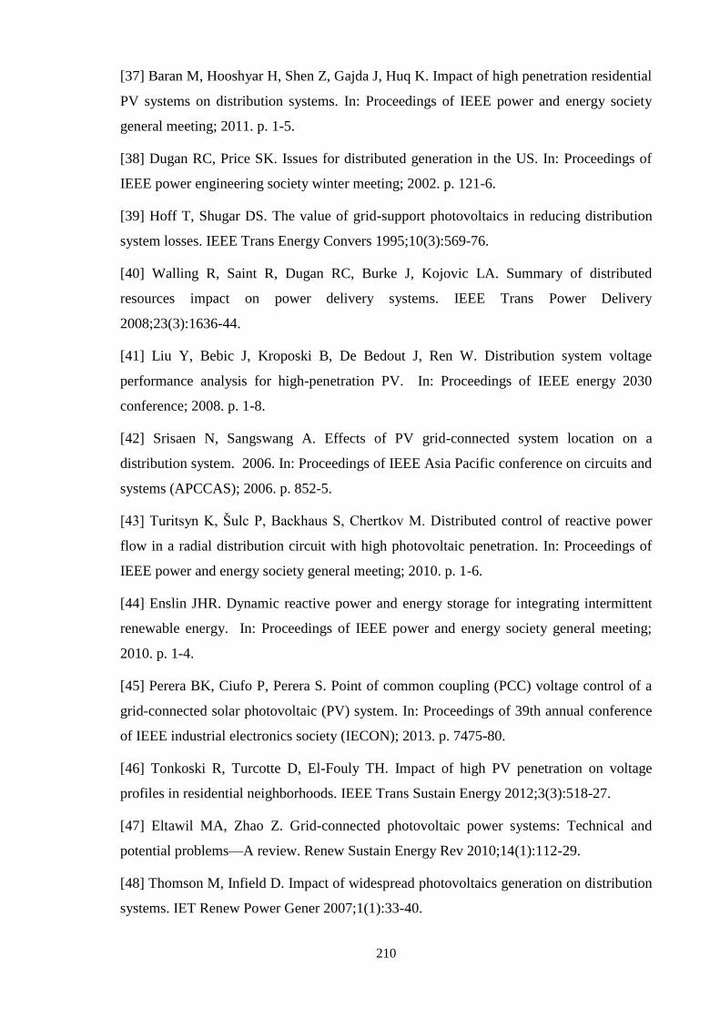
210

[37] Baran M, Hooshyar H, Shen Z, Gajda J, Huq K. Impact of high penetration residential

PV systems on distribution systems. In: Proceedings of IEEE power and energy society

general meeting; 2011. p. 1-5.

[38] Dugan RC, Price SK. Issues for distributed generation in the US. In: Proceedings of

IEEE power engineering society winter meeting; 2002. p. 121-6.

[39] Hoff T, Shugar DS. The value of grid-support photovoltaics in reducing distribution

system losses. IEEE Trans Energy Convers 1995;10(3):569-76.

[40] Walling R, Saint R, Dugan RC, Burke J, Kojovic LA. Summary of distributed

resources impact on power delivery systems. IEEE Trans Power Delivery

2008;23(3):1636-44.

[41] Liu Y, Bebic J, Kroposki B, De Bedout J, Ren W. Distribution system voltage

performance analysis for high-penetration PV. In: Proceedings of IEEE energy 2030

conference; 2008. p. 1-8.

[42] Srisaen N, Sangswang A. Effects of PV grid-connected system location on a

distribution system. 2006. In: Proceedings of IEEE Asia Pacific conference on circuits and

systems (APCCAS); 2006. p. 852-5.

[43] Turitsyn K, Šulc P, Backhaus S, Chertkov M. Distributed control of reactive power

flow in a radial distribution circuit with high photovoltaic penetration. In: Proceedings of

IEEE power and energy society general meeting; 2010. p. 1-6.

[44] Enslin JHR. Dynamic reactive power and energy storage for integrating intermittent

renewable energy. In: Proceedings of IEEE power and energy society general meeting;

2010. p. 1-4.

[45] Perera BK, Ciufo P, Perera S. Point of common coupling (PCC) voltage control of a

grid-connected solar photovoltaic (PV) system. In: Proceedings of 39th annual conference

of IEEE industrial electronics society (IECON); 2013. p. 7475-80.

[46] Tonkoski R, Turcotte D, El-Fouly TH. Impact of high PV penetration on voltage

profiles in residential neighborhoods. IEEE Trans Sustain Energy 2012;3(3):518-27.

[47] Eltawil MA, Zhao Z. Grid-connected photovoltaic power systems: Technical and

potential problems—A review. Renew Sustain Energy Rev 2010;14(1):112-29.

[48] Thomson M, Infield D. Impact of widespread photovoltaics generation on distribution

systems. IET Renew Power Gener 2007;1(1):33-40.

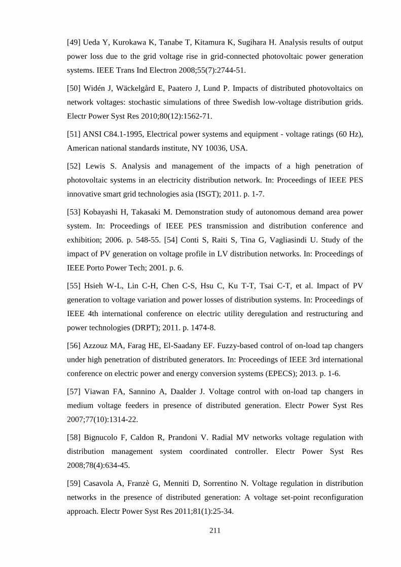
211

[49] Ueda Y, Kurokawa K, Tanabe T, Kitamura K, Sugihara H. Analysis results of output

power loss due to the grid voltage rise in grid-connected photovoltaic power generation

systems. IEEE Trans Ind Electron 2008;55(7):2744-51.

[50] Widén J, Wäckelgård E, Paatero J, Lund P. Impacts of distributed photovoltaics on

network voltages: stochastic simulations of three Swedish low-voltage distribution grids.

Electr Power Syst Res 2010;80(12):1562-71.

[51] ANSI C84.1-1995, Electrical power systems and equipment - voltage ratings (60 Hz),

American national standards institute, NY 10036, USA.

[52] Lewis S. Analysis and management of the impacts of a high penetration of

photovoltaic systems in an electricity distribution network. In: Proceedings of IEEE PES

innovative smart grid technologies asia (ISGT); 2011. p. 1-7.

[53] Kobayashi H, Takasaki M. Demonstration study of autonomous demand area power

system. In: Proceedings of IEEE PES transmission and distribution conference and

exhibition; 2006. p. 548-55. [54] Conti S, Raiti S, Tina G, Vagliasindi U. Study of the

impact of PV generation on voltage profile in LV distribution networks. In: Proceedings of

IEEE Porto Power Tech; 2001. p. 6.

[55] Hsieh W-L, Lin C-H, Chen C-S, Hsu C, Ku T-T, Tsai C-T, et al. Impact of PV

generation to voltage variation and power losses of distribution systems. In: Proceedings of

IEEE 4th international conference on electric utility deregulation and restructuring and

power technologies (DRPT); 2011. p. 1474-8.

[56] Azzouz MA, Farag HE, El-Saadany EF. Fuzzy-based control of on-load tap changers

under high penetration of distributed generators. In: Proceedings of IEEE 3rd international

conference on electric power and energy conversion systems (EPECS); 2013. p. 1-6.

[57] Viawan FA, Sannino A, Daalder J. Voltage control with on-load tap changers in

medium voltage feeders in presence of distributed generation. Electr Power Syst Res

2007;77(10):1314-22.

[58] Bignucolo F, Caldon R, Prandoni V. Radial MV networks voltage regulation with

distribution management system coordinated controller. Electr Power Syst Res

2008;78(4):634-45.

[59] Casavola A, Franzè G, Menniti D, Sorrentino N. Voltage regulation in distribution

networks in the presence of distributed generation: A voltage set-point reconfiguration

approach. Electr Power Syst Res 2011;81(1):25-34.

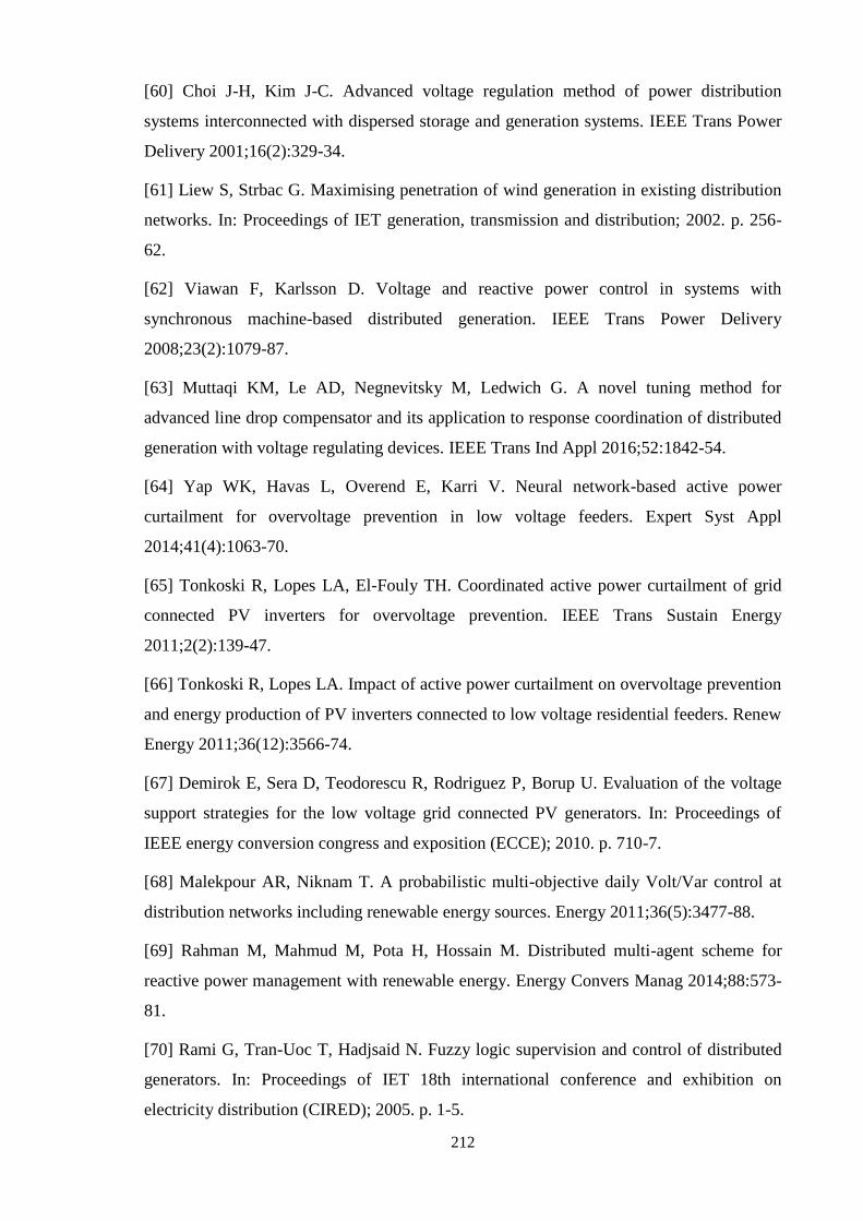
212

[60] Choi J-H, Kim J-C. Advanced voltage regulation method of power distribution

systems interconnected with dispersed storage and generation systems. IEEE Trans Power

Delivery 2001;16(2):329-34.

[61] Liew S, Strbac G. Maximising penetration of wind generation in existing distribution

networks. In: Proceedings of IET generation, transmission and distribution; 2002. p. 256-

62.

[62] Viawan F, Karlsson D. Voltage and reactive power control in systems with

synchronous machine-based distributed generation. IEEE Trans Power Delivery

2008;23(2):1079-87.

[63] Muttaqi KM, Le AD, Negnevitsky M, Ledwich G. A novel tuning method for

advanced line drop compensator and its application to response coordination of distributed

generation with voltage regulating devices. IEEE Trans Ind Appl 2016;52:1842-54.

[64] Yap WK, Havas L, Overend E, Karri V. Neural network-based active power

curtailment for overvoltage prevention in low voltage feeders. Expert Syst Appl

2014;41(4):1063-70.

[65] Tonkoski R, Lopes LA, El-Fouly TH. Coordinated active power curtailment of grid

connected PV inverters for overvoltage prevention. IEEE Trans Sustain Energy

2011;2(2):139-47.

[66] Tonkoski R, Lopes LA. Impact of active power curtailment on overvoltage prevention

and energy production of PV inverters connected to low voltage residential feeders. Renew

Energy 2011;36(12):3566-74.

[67] Demirok E, Sera D, Teodorescu R, Rodriguez P, Borup U. Evaluation of the voltage

support strategies for the low voltage grid connected PV generators. In: Proceedings of

IEEE energy conversion congress and exposition (ECCE); 2010. p. 710-7.

[68] Malekpour AR, Niknam T. A probabilistic multi-objective daily Volt/Var control at

distribution networks including renewable energy sources. Energy 2011;36(5):3477-88.

[69] Rahman M, Mahmud M, Pota H, Hossain M. Distributed multi-agent scheme for

reactive power management with renewable energy. Energy Convers Manag 2014;88:573-

81.

[70] Rami G, Tran-Uoc T, Hadjsaid N. Fuzzy logic supervision and control of distributed

generators. In: Proceedings of IET 18th international conference and exhibition on

electricity distribution (CIRED); 2005. p. 1-5.

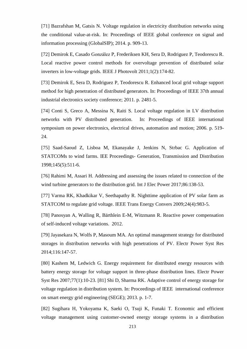
213

[71] Bazrafshan M, Gatsis N. Voltage regulation in electricity distribution networks using

the conditional value-at-risk. In: Proceedings of IEEE global conference on signal and

information processing (GlobalSIP); 2014. p. 909-13.

[72] Demirok E, Casado Gonz lez P, Frederiksen KH, Sera D, Rodriguez P, Teodorescu R.

Local reactive power control methods for overvoltage prevention of distributed solar

inverters in low-voltage grids. IEEE J Photovolt 2011;1(2):174-82.

[73] Demirok E, Sera D, Rodriguez P, Teodorescu R. Enhanced local grid voltage support

method for high penetration of distributed generators. In: Proceedings of IEEE 37th annual

industrial electronics society conference; 2011. p. 2481-5.

[74] Conti S, Greco A, Messina N, Raiti S. Local voltage regulation in LV distribution

networks with PV distributed generation. In: Proceedings of IEEE international

symposium on power electronics, electrical drives, automation and motion; 2006. p. 519-

24.

[75] Saad-Saoud Z, Lisboa M, Ekanayake J, Jenkins N, Strbac G. Application of

STATCOMs to wind farms. IEE Proceedings- Generation, Transmission and Distribution

1998;145(5):511-6.

[76] Rahimi M, Assari H. Addressing and assessing the issues related to connection of the

wind turbine generators to the distribution grid. Int J Elec Power 2017;86:138-53.

[77] Varma RK, Khadkikar V, Seethapathy R. Nighttime application of PV solar farm as

STATCOM to regulate grid voltage. IEEE Trans Energy Convers 2009;24(4):983-5.

[78] Panosyan A, Walling R, Bärthlein E-M, Witzmann R. Reactive power compensation

of self-induced voltage variations. 2012.

[79] Jayasekara N, Wolfs P, Masoum MA. An optimal management strategy for distributed

storages in distribution networks with high penetrations of PV. Electr Power Syst Res

2014;116:147-57.

[80] Kashem M, Ledwich G. Energy requirement for distributed energy resources with

battery energy storage for voltage support in three-phase distribution lines. Electr Power

Syst Res 2007;77(1):10-23. [81] Shi D, Sharma RK. Adaptive control of energy storage for

voltage regulation in distribution system. In: Proceedings of IEEE international conference

on smart energy grid engineering (SEGE); 2013. p. 1-7.

[82] Sugihara H, Yokoyama K, Saeki O, Tsuji K, Funaki T. Economic and efficient

voltage management using customer-owned energy storage systems in a distribution

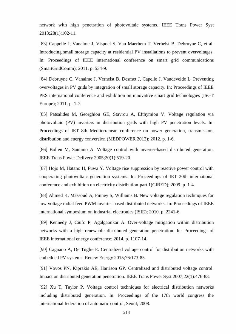
214

network with high penetration of photovoltaic systems. IEEE Trans Power Syst

2013;28(1):102-11.

[83] Cappelle J, Vanalme J, Vispoel S, Van Maerhem T, Verhelst B, Debruyne C, et al.

Introducing small storage capacity at residential PV installations to prevent overvoltages.

In: Proceedings of IEEE international conference on smart grid communications

(SmartGridComm); 2011. p. 534-9.

[84] Debruyne C, Vanalme J, Verhelst B, Desmet J, Capelle J, Vandevelde L. Preventing

overvoltages in PV grids by integration of small storage capacity. In: Proceedings of IEEE

PES international conference and exhibition on innovative smart grid technologies (ISGT

Europe); 2011. p. 1-7.

[85] Patsalides M, Georghiou GE, Stavrou A, Efthymiou V. Voltage regulation via

photovoltaic (PV) inverters in distribution grids with high PV penetration levels. In:

Proceedings of IET 8th Mediterranean conference on power generation, transmission,

distribution and energy conversion (MEDPOWER 2012); 2012. p. 1-6.

[86] Bollen M, Sannino A. Voltage control with inverter-based distributed generation.

IEEE Trans Power Delivery 2005;20(1):519-20.

[87] Hojo M, Hatano H, Fuwa Y. Voltage rise suppression by reactive power control with

cooperating photovoltaic generation systems. In: Proceedings of IET 20th international

conference and exhibition on electricity distribution-part 1(CIRED); 2009. p. 1-4.

[88] Ahmed K, Massoud A, Finney S, Williams B. New voltage regulation techniques for

low voltage radial feed PWM inverter based distributed networks. In: Proceedings of IEEE

international symposium on industrial electronics (ISIE); 2010. p. 2241-6.

[89] Kennedy J, Ciufo P, Agalgaonkar A. Over-voltage mitigation within distribution

networks with a high renewable distributed generation penetration. In: Proceedings of

IEEE international energy conference; 2014. p. 1107-14.

[90] Cagnano A, De Tuglie E. Centralized voltage control for distribution networks with

embedded PV systems. Renew Energy 2015;76:173-85.

[91] Vovos PN, Kiprakis AE, Harrison GP. Centralized and distributed voltage control:

Impact on distributed generation penetration. IEEE Trans Power Syst 2007;22(1):476-83.

[92] Xu T, Taylor P. Voltage control techniques for electrical distribution networks

including distributed generation. In: Proceedings of the 17th world congress the

international federation of automatic control, Seoul; 2008.

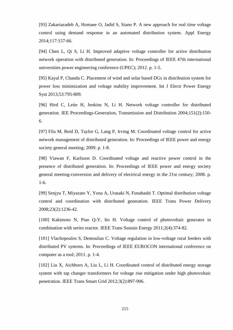
215

[93] Zakariazadeh A, Homaee O, Jadid S, Siano P. A new approach for real time voltage

control using demand response in an automated distribution system. Appl Energy

2014;117:157-66.

[94] Chen L, Qi S, Li H. Improved adaptive voltage controller for active distribution

network operation with distributed generation. In: Proceedings of IEEE 47th international

universities power engineering conference (UPEC); 2012. p. 1-5.

[95] Kayal P, Chanda C. Placement of wind and solar based DGs in distribution system for

power loss minimization and voltage stability improvement. Int J Electr Power Energy

Syst 2013;53:795-809.

[96] Hird C, Leite H, Jenkins N, Li H. Network voltage controller for distributed

generation. IEE Proceedings-Generation, Transmission and Distribution 2004;151(2):150-

6.

[97] Fila M, Reid D, Taylor G, Lang P, Irving M. Coordinated voltage control for active

network management of distributed generation. In: Proceedings of IEEE power and energy

society general meeting; 2009. p. 1-8.

[98] Viawan F, Karlsson D. Coordinated voltage and reactive power control in the

presence of distributed generation. In: Proceedings of IEEE power and energy society

general meeting-conversion and delivery of electrical energy in the 21st century; 2008. p.

1-6.

[99] Senjyu T, Miyazato Y, Yona A, Urasaki N, Funabashi T. Optimal distribution voltage

control and coordination with distributed generation. IEEE Trans Power Delivery

2008;23(2):1236-42.

[100] Kakimoto N, Piao Q-Y, Ito H. Voltage control of photovoltaic generator in

combination with series reactor. IEEE Trans Sustain Energy 2011;2(4):374-82.

[101] Vlachopoulos S, Demoulias C. Voltage regulation in low-voltage rural feeders with

distributed PV systems. In: Proceedings of IEEE EUROCON international conference on

computer as a tool; 2011. p. 1-4.

[102] Liu X, Aichhorn A, Liu L, Li H. Coordinated control of distributed energy storage

system with tap changer transformers for voltage rise mitigation under high photovoltaic

penetration. IEEE Trans Smart Grid 2012;3(2):897-906.

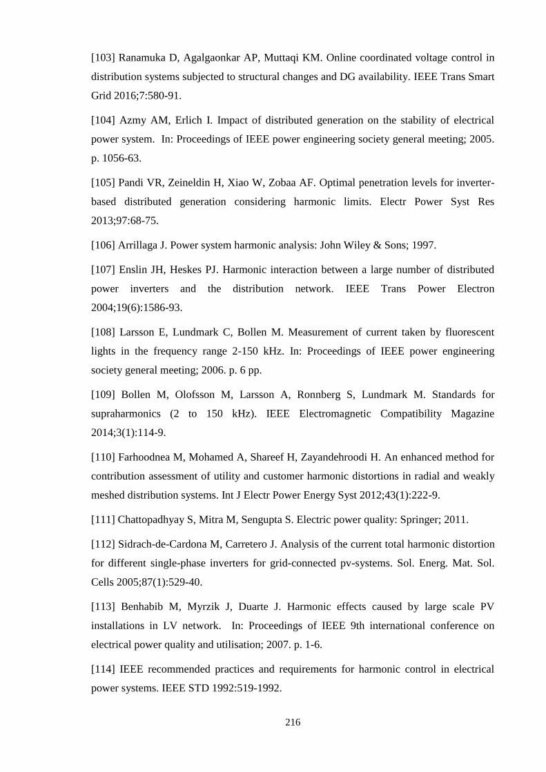
216

[103] Ranamuka D, Agalgaonkar AP, Muttaqi KM. Online coordinated voltage control in

distribution systems subjected to structural changes and DG availability. IEEE Trans Smart

Grid 2016;7:580-91.

[104] Azmy AM, Erlich I. Impact of distributed generation on the stability of electrical

power system. In: Proceedings of IEEE power engineering society general meeting; 2005.

p. 1056-63.

[105] Pandi VR, Zeineldin H, Xiao W, Zobaa AF. Optimal penetration levels for inverter-

based distributed generation considering harmonic limits. Electr Power Syst Res

2013;97:68-75.

[106] Arrillaga J. Power system harmonic analysis: John Wiley & Sons; 1997.

[107] Enslin JH, Heskes PJ. Harmonic interaction between a large number of distributed

power inverters and the distribution network. IEEE Trans Power Electron

2004;19(6):1586-93.

[108] Larsson E, Lundmark C, Bollen M. Measurement of current taken by fluorescent

lights in the frequency range 2-150 kHz. In: Proceedings of IEEE power engineering

society general meeting; 2006. p. 6 pp.

[109] Bollen M, Olofsson M, Larsson A, Ronnberg S, Lundmark M. Standards for

supraharmonics (2 to 150 kHz). IEEE Electromagnetic Compatibility Magazine

2014;3(1):114-9.

[110] Farhoodnea M, Mohamed A, Shareef H, Zayandehroodi H. An enhanced method for

contribution assessment of utility and customer harmonic distortions in radial and weakly

meshed distribution systems. Int J Electr Power Energy Syst 2012;43(1):222-9.

[111] Chattopadhyay S, Mitra M, Sengupta S. Electric power quality: Springer; 2011.

[112] Sidrach-de-Cardona M, Carretero J. Analysis of the current total harmonic distortion

for different single-phase inverters for grid-connected pv-systems. Sol. Energ. Mat. Sol.

Cells 2005;87(1):529-40.

[113] Benhabib M, Myrzik J, Duarte J. Harmonic effects caused by large scale PV

installations in LV network. In: Proceedings of IEEE 9th international conference on

electrical power quality and utilisation; 2007. p. 1-6.

[114] IEEE recommended practices and requirements for harmonic control in electrical

power systems. IEEE STD 1992:519-1992.

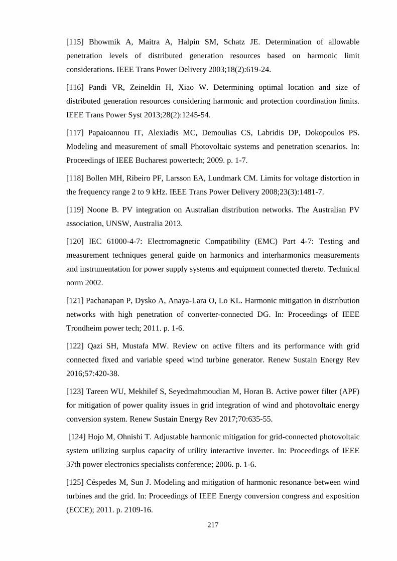
217

[115] Bhowmik A, Maitra A, Halpin SM, Schatz JE. Determination of allowable

penetration levels of distributed generation resources based on harmonic limit

considerations. IEEE Trans Power Delivery 2003;18(2):619-24.

[116] Pandi VR, Zeineldin H, Xiao W. Determining optimal location and size of

distributed generation resources considering harmonic and protection coordination limits.

IEEE Trans Power Syst 2013;28(2):1245-54.

[117] Papaioannou IT, Alexiadis MC, Demoulias CS, Labridis DP, Dokopoulos PS.

Modeling and measurement of small Photovoltaic systems and penetration scenarios. In:

Proceedings of IEEE Bucharest powertech; 2009. p. 1-7.

[118] Bollen MH, Ribeiro PF, Larsson EA, Lundmark CM. Limits for voltage distortion in

the frequency range 2 to 9 kHz. IEEE Trans Power Delivery 2008;23(3):1481-7.

[119] Noone B. PV integration on Australian distribution networks. The Australian PV

association, UNSW, Australia 2013.

[120] IEC 61000-4-7: Electromagnetic Compatibility (EMC) Part 4-7: Testing and

measurement techniques general guide on harmonics and interharmonics measurements

and instrumentation for power supply systems and equipment connected thereto. Technical

norm 2002.

[121] Pachanapan P, Dysko A, Anaya-Lara O, Lo KL. Harmonic mitigation in distribution

networks with high penetration of converter-connected DG. In: Proceedings of IEEE

Trondheim power tech; 2011. p. 1-6.

[122] Qazi SH, Mustafa MW. Review on active filters and its performance with grid

connected fixed and variable speed wind turbine generator. Renew Sustain Energy Rev

2016;57:420-38.

[123] Tareen WU, Mekhilef S, Seyedmahmoudian M, Horan B. Active power filter (APF)

for mitigation of power quality issues in grid integration of wind and photovoltaic energy

conversion system. Renew Sustain Energy Rev 2017;70:635-55.

[124] Hojo M, Ohnishi T. Adjustable harmonic mitigation for grid-connected photovoltaic

system utilizing surplus capacity of utility interactive inverter. In: Proceedings of IEEE

37th power electronics specialists conference; 2006. p. 1-6.

[125] Céspedes M, Sun J. Modeling and mitigation of harmonic resonance between wind

turbines and the grid. In: Proceedings of IEEE Energy conversion congress and exposition

(ECCE); 2011. p. 2109-16.

218

[126] Carastro F, Sumner M, Zanchetta P. Mitigation of voltage dips and voltage

harmonics within a micro-grid, using a single shunt active filter with energy storage. In:

Proceedings of IEEE 32nd annual conference on industrial electronics; 2006. p. 2546-51.

[127] Yong B, Ramachandaramurthy V. Double Tuned filter design for harmonic

mitigation in grid connected solar PV. In: Proceedings of IEEE international conference on

power and energy (PECon); 2014. p. 293-7.

[128] Savaghebi M, Guerrero JM, Jalilian A, Vasquez JC. Mitigation of voltage and

current harmonics in grid-connected microgrids. In: Proceedings of IEEE international

symposium on industrial electronics (ISIE); 2012. p. 1610-5.

[129] Pogaku N, Green T. Harmonic mitigation throughout a distribution system: a

distributed-generator-based solution. IEE Proceedings- Gener, Transm Distrib

2006;153(3):350-8.

[130] Moreno R, Pomilio J, Da Silva LP, Pimentel S. Mitigation of harmonic distortion by

power electronic interface connecting distributed generation sources to a weak grid. In:

Proceedings of IEEE Brazilian power electronics conference; 2009. p. 41-8.

[131] Kulkarni A, John V. Mitigation of lower order harmonics in a grid-connected single-

phase PV inverter. IEEE Trans Power Electron 2013;28(11):5024-37.

[132] Hazrati A, Jalilian A. Grid side power quality enhancement in DFIG based grid

connected wind plants. In: Proceedings of IEEE 17th conference on electrical power

distribution networks; 2012. p. 1-7.

[133] Liang X, Emerging power quality challenges due to integration of renewable energy

sources. IEEE Trans Ind Appl 2016.

[134] Bollen MH, Stockman K, Neumann R, Ethier G, Gordon JR, Van Reussel K, et al.

Voltage dip immunity of equipment and installations-messages to stakeholders. In:

Proceedings of IEEE15th international conference on harmonics and quality of power

(ICHQP); 2012. p. 915-9.

[135] Martinez-Velasco J, Martin-Arnedo J. Distributed generation impact on voltage sags

in distribution networks. In: Proceedings of IEEE 9th international conference on electrical

power quality and utilisation; 2007. p. 1-6.

[136] Alvarez C, Amarís H, Samuelsson O. Voltage dip mitigation at wind farms. In:

Proceedings of IEEE European wind energy conference; 2007.

219

[137] Eskander MN, Amer SI. Mitigation of voltage dips and swells in grid-connected

wind energy conversion systems. IETE J Res 2011;57(6):515-24.

[138] Hossam-Eldin A, Elserougi A. Renewable energy fed inter-line dvr for voltage sag

mitigation in distribution grids. 2013.

[139] Renders B, De Gussemé K, Ryckaert WR, Stockman K, Vandevelde L, Bollen MH.

Distributed generation for mitigating voltage dips in low-voltage distribution grids. IEEE

Trans Power Delivery 2008;23(3):1581-8.

[140] Trindade FC, do Nascimento KV, Vieira JC. Investigation on voltage sags caused by

DG anti-islanding protection. IEEE Trans Power Delivery 2013;28(2):972-80.

[141] Jowder F. Design and analysis of dynamic voltage restorer for deep voltage sag and

harmonic compensation. IET Gener, Transm Distrib 2009;3(6):547-60.

[142] Biswas S, Goswami SK, Chatterjee A. Optimum distributed generation placement

with voltage sag effect minimization. Energy Convers Manag 2012;53(1):163-74.

[143] Kaddah SS, El-Saadawi MM, El-Hassanin DM. Influence of distributed generation

on distribution networks during faults. Electr Power Compon Syst 2015; 43(16): 1781-

1792.

[144] Ipinnimo O, Chowdhury S, Chowdhury S. Application of grid integrated wind

energy conversion systems for mitigation of multiple voltage dips in a power network. In:

Proceedings of IEEE 46th international universities power engineering conference

(UPEC); 2011. p. 1-6.

[145] Macken KJ, Bollen MH, Belmans RJ. Mitigation of voltage dips through distributed

generation systems. In: Proceedings of IEEE 38th annual meeting industry applications

conference; 2003. p. 1068-74.

[146] Song-cen W, Kun-Shan Y, Guang-fu T. Mitigation of voltage sags by grid-connected

distributed generation system in series and shunt configurations. In: Proceedings of IEEE

joint international conference on power system technology and IEEE power India

conference; 2008. p. 1-6.

[147] Wasiak I, Mienski R, Pawelek R, Gburczyk P. Application of DSTATCOM

compensators for mitigation of power quality disturbances in low voltage grid with

distributed generation. In: Proceedings of IEEE 9th international conference on electrical

power quality and utilisation; 2007. p. 1-6.

220

[148] Magueed F, Awad H. Voltage compensation in weak grids using distributed

generation with voltage source converter as a front end. In: Proceedings of IEEE

international conference on power electronics and drives systems; 2005. p. 234-9.

[149] Cataliotti A, Cocchiara G, Ippolito MG, Morana G. Applications of the fault

decoupling device to improve the operation of LV distribution networks. IEEE Trans

Power Delivery 2008;23(1):328-37.

[150] Amanifar O, Golshan MEH. Optimal DG allocation and sizing for mitigating voltage

sag in distribution systems with respect to economic consideration using Particle Swarm

Optimization. In: Proceedings of IEEE 17th conference on electrical power distribution

networks (EPDC); 2012. p. 1-8.

[151] Banaei M, Hosseini S, Khajee MD. Mitigation of voltage sag using adaptive neural

network with dynamic voltage restorer. In: Proceedings of IEEE 5th international power

electronics and motion control conference; 2006. p. 1-5.

[152] Van TL, Nguyen TH, Lee D-C. Flicker mitigation in DFIG wind turbine systems. In:

Proceedings of IEEE 14th European conference on power electronics and applications;

2011. p. 1-10.

[153] Zheng T, Makram EB. Wavelet representation of voltage flicker. Electr Power Syst

Res 1998;48(2):133-40.

[154] Hernández J, Ortega M, De la Cruz J, Vera D. Guidelines for the technical

assessment of harmonic, flicker and unbalance emission limits for PV-distributed

generation. Electr Power Syst Res 2011;81(7):1247-57.

[155] El-Samahy I, El-Saadany E. The effect of DG on power quality in a deregulated

environment. In: Proceedings of IEEE power engineering society general meeting; 2005.

p. 2969-76.

[156] Ding T, Kou Y, Yang Y, Zhang Y, Yan H, Blaabjerg F. Evaluating maximum

photovoltaic integration in district distribution systems considering optimal inverter

dispatch and cloud shading conditions. IET Renew Power Gener 2016.

[157] Gulachenski E, Kern Jr E, Feero W, Emanuel A. Photovoltaic generation effects on

distribution feeders. Electric Power Research Inst., Palo Alto, CA (United States); New

England Power Service Co., Westborough, MA (United States); Ascension Technology,

Lincoln Center, MA (United States); Electric Research and Management, Inc., State

College, PA (United States); Worcester Polytechnic Inst., MA (United States); 1991.

221

[158] Woyte A, Van Thong V, Belmans R, Nijs J. Voltage fluctuations on distribution

level introduced by photovoltaic systems. IEEE Trans Energy Convers 2006;21(1):202-9.

[159] Ari G, Baghzouz Y. Impact of high PV penetration on voltage regulation in electrical

distribution systems. In: Proceedings of IEEE international conference on clean electrical

power (ICCEP); 2011. p. 744-8.

[160] Tan Y, Kirschen D, Jenkins N. Impact of a Large Penetration of Photovoltaic

Generation on the PowerSystem. In: Proceedings of IEEE Barcelona 17th international

conference on electricity distribution; 2003. p. 12-5.

[161] Borlase S. Smart grids: infrastructure, technology, and solutions: CRC Press; 2012.

[162] Jewell WT, Unruh TD. Limits on cloud-induced fluctuation in photovoltaic

generation. IEEE Trans Energy Convers 1990;5(1):8-14.

[163] Jewell W, Ramakumar R. The effects of moving clouds on electric utilities with

dispersed photovoltaic generation. IEEE Trans Energy Convers 1987(4):570-6.

[164] Blooming TM, Carnovale DJ. Application of IEEE Std 519-1992 harmonic limits.

In: Proceedings of IEEE annual pulp and paper industry technical conference; 2006. p. 1-9.

[165] Sun J, Czarkowski D, Zabar Z. Voltage flicker mitigation using PWM-based

distribution STATCOM. In: Proceedings of IEEE power engineering society summer

meeting; 2002. p. 616-21.

[166] Jenner M, Brockhurst FC. Vacuum switched capacitors to reduce induction motor

caused voltage flicker on a 12.47 kV rural distribution line. In: Proceedings of IEEE 34th

annual rural electric power conference; 1990. p. B5/1-B5/.

[167] Virulkar VB, Aware MV. Voltage Flicker Mitigation Using STATCOM and ESS.

In: Proceedings of IEEE joint international conference on power system technology and

IEEE power India conference; 2008. p. 1-7.

[168] Naka S, Genji T, Yura T, Takayama S, Hayashi N, Tokuda H, et al. Cooperative

control method for voltage control equipment considering interconnection of distributed

generators. In: Proceedings of IEEE international conference on electrical engineering

(ICEE), Xi'an, China;2001.

[169] Qi Y, Jia H. Research on a new voltage control strategy for photovoltaic grid-

connected system. In: Proceedings of IEEE international conference on electrical machines

and systems (ICEMS); 2011. p. 1-6.

222

[170] Wong J, Lim YS, Morris E. Novel fuzzy controlled energy storage for low-voltage

distribution networks with photovoltaic systems under highly cloudy conditions. J Energy

Eng 2014.

[171] Shivashankar S, Mekhilef S, Mokhlis M, Karimi M, Mitigating methods of power

fluctuation of photovoltaic (PV) sources–A review. Renew Sustain Energy Rev

2016;59:1170-84.

[172] Machmoum M, Hatoum A, Bouaouiche T. Flicker mitigation in a doubly fed

induction generator wind turbine system. Math Comput Simul 2010;81(2):433-45.

[173] Meegahapola L, Fox B, Flynn D. Flicker mitigation strategy for DFIGs during

variable wind conditions. In: Proceedings of IEEE power and energy society general

meeting; 2010. p. 1-8.

[174] Sun T. Power quality of grid-connected wind turbines with DFIG and their

interaction with the grid: Institute of Energy Tecnology, Aalborg University; 2004.

[175] Sun T, Chen Z, Blaabjerg F. Flicker study on variable speed wind turbines with

doubly fed induction generators. IEEE Trans Energy Convers 2005;20(4):896-905.

[176] Zhang Y, Hu W, Chen Z, Cheng M. Mitigation of wind power fluctuation by active

current control of variable speed wind turbines. Int J Smart Grid Clean Energy

2013;2(2):252-7.

[177] Ammar M, Joos G. Flicker mitigation planning solutions in distributed wind power:

A real-time simulation analysis. In: Proceedings of IEEE international conference on

renewable energy research and application (ICRERA); 2014. p. 284-8.

[178] Von Jouanne A, Banerjee B. Assessment of voltage unbalance. IEEE Trans Power

Delivery 2001;16(4):782-90.

[179] Shahnia F, Majumder R, Ghosh A, Ledwich G, Zare F. Voltage imbalance analysis

in residential low voltage distribution networks with rooftop PVs. Electr Power Syst Res

2011;81(9):1805-14.

[180] Meersman B, Renders B, Degroote L, Vandoorn T, Vandevelde L. Three-phase

inverter-connected DG-units and voltage unbalance. Electr Power Syst Res

2011;81(4):899-906.

[181] Hosseini SH, Nazarloo A. Voltage unbalance reduction by distribution static

compensator in a case study network. In: Proceedings of IEEE 7th international conference

on electrical and electronics engineering (ELECO); 2011. p. I-288-I-92.

223

[182] Graovac D, Katić V, Rufer A. Power quality problems compensation with universal

power quality conditioning system. IEEE Trans Power Delivery 2007;22(2):968-76.

[183] Wong J, Seng Lim Y, Morris E. Distributed energy storage systems with an

improved fuzzy controller for mitigating voltage unbalance on low-voltage networks. J

Energy Eng 2014:04014058.

[184] Chua KH, Wong J, Lim YS, Taylor P, Morris E, Morris S. Mitigation of voltage

unbalance in low voltage distribution network with high level of photovoltaic system.

Energy Procedia 2011;12:495-501.

[185] Cziker A, Chindris M, Miron A. Voltage unbalance mitigation using a distributed

generator. In: Proceedings of IEEE 11th International conference on optimization of

electrical and electronic equipment; 2008. p. 221-6.

[186] Gerdes G, Santjer F. Power quality of wind turbines and their interaction with the

grid. American wind energy association, Washington DC (United States); 1995.

[187] A Attya A, Hartkopf T. Control and quantification of kinetic energy released by

wind farms during power system frequency drops. IET Renew Power Gener

2013;7(3):210-24.

[188] Yan R, Saha TK, Modi N, Masood N-A, Mosadeghy M. The combined effects of

high penetration of wind and PV on power system frequency response. Appl Energy

2015;145:320-30.

[189] Rahmann C, Castillo A. Fast frequency response capability of photovoltaic power

plants: The necessity of new grid requirements and definitions. Energies 2014;7(10):6306-

22.

[190] International Electrotechnical Commission (IEC) 61727 - Photovoltaic (PV) systems

- Characteristics of the utility interface. 2004.

[191] Kumar P, Kothari DP. Recent philosophies of automatic generation control strategies

in power systems. IEEE Trans Power Syst 2005;20(1):346-57.

[192] Chang L, Kojabadi HM. Review of interconnection standards for distributed power

generation. In: Proceedings of IEEE large engineering systems conference on power

engineering (LESCOPE); 2002. p. 36-40.

[193] Pandey SK, Mohanty SR, Kishor N. A literature survey on load–frequency control

for conventional and distribution generation power systems. Renew Sustain Energy Rev

2013; 25:318-34.

224

[194] Liu X, Zhang Y, Lee KY. Coordinated Distributed MPC for Load Frequency

Control of Power System with Wind Farms. IEEE Trans Ind Electr 2016.

[195] Shayeghi H, Shayanfar H, Jalili A. Load frequency control strategies: A state-of-the-

art survey for the researcher. Energy Convers Manag 2009;50(2):344-53.

[196] Conti S. Analysis of distribution network protection issues in presence of dispersed

generation. Electr Power Syst Res 2009;79(1):49-56.

[197] Girgis A, Brahma S. Effect of distributed generation on protective device

coordination in distribution system. In: Proceedings of IEEE large engineering systems

conference on power engineering; 2001. p. 115-9.

[198] Boljevic S, Conlon MF. The contribution to distribution network short-circuit current

level from the connection of distributed generation. In: Proceedings of IEEE 3rd

international universities power engineering conference; 2008. p. 1-6.

[199] Boutsika TN, Papathanassiou SA. Short-circuit calculations in networks with

distributed generation. Electr Power Syst Res 2008;78(7):1181-91.

[200] Tan S, Salman S. Investigation into the implementation of auto reclosing scheme in

distribution networks with high penetration of DGs. In: Proceedings of IEEE 43rd

international universities power engineering conference; 2008. p. 1-5.

[201] Bründlinger R, Bletterie B. Unintentional islanding in distribution grids with a high

penetration of inverter-based DG: Probability for islanding and protection methods. In:

Proceedings of IEEE Russia power tech; 2005. p. 1-7.

[202] Menon V, Nehrir MH. A hybrid islanding detection technique using voltage

unbalance and frequency set point. IEEE Trans Power Syst 2007;22(1):442-8.

[203] Khamis A, Shareef H, Bizkevelci E, Khatib T. A review of islanding detection

techniques for renewable distributed generation systems. Renew Sustain Energy Rev

2013;28:483-93.

[204] Chowdhury S, Chowdhury S, Crossley P. Islanding protection of active distribution

networks with renewable distributed generators: A comprehensive survey. Electr Power

Syst Res 2009;79(6):984-92.

[205] Zayandehroodi H, Mohamed A, Shareef H, Mohammadjafari M. A Comprehensive

review of protection coordination methods in power distribution systems in the presence of

DG. Electr Rev 2011(8):142-8.

225

[206] Kennedy J, Ciufo P, Agalgaonkar A. A review of protection systems for distribution

networks embedded with renewable generation. Renew Sustain Energy Rev 2016;58:1308-

17.

[207] Dugan RC. Reference guide: the open distribution system simulator (opendss).

Electric Power Research Institute, Inc 2012.

[208] Tang Y, Mao X, Ayyanar R. Distribution system modeling using CYMDIST for

study of high penetration of distributed solar photovoltaics. In: Proceedings of IEEE North

American power symposium (NAPS); 2012. p. 1-6.

[209] Siemens A, PTI E. PSS® SINCAL Version 6.0. November; 2009.

[210] Manual DPF, PowerFactory D. Version 14.0. DIgSILENT GmbH, Gomaringen,

Germany 2009.

[211] Chassin D, Schneider K, Gerkensmeyer C. GridLAB-D: An open-source power

systems modeling and simulation environment. In: Proceedings of IEEE/PES transmission

and distribution conference and exposition;2008.

[212] Milano F, Vanfretti L, Morataya JC. An open source power system virtual

laboratory: The PSAT case and experience. IEEE Trans Edu 2008;51(1):17-23.

[213] Consortium D. 4DIAC–Framework for Distributed Industrial Automation and

Control, Open Source Initiative. access date October 2007.

[214] Moffet M-A, Sirois F, Beauvais D. Review of open-source code power grid

simulation tools for long-term parametic simulation. CanmetENERGY, TR–2011‐137

(RP‐TEC) 411‐MODSIM 2011. [215] Ortmeyer T, Dugan R, Crudele D, Key T, Barker P.

Renewable systems interconnection study: utility models, analysis, and simulation tools.

Sandia NM: Sandia National Laboratory Report: SAND2008‐0945 P, February 2008.

[216] Martinez J, De León F, Mehrizi-Sani A, Nehrir M, Wang C, Dinavahi V. Tools for

analysis and design of distributed resources—Part II: Tools for planning, analysis and

design of distribution networks with distributed resources. IEEE Trans Power Delivery

2011;26(3):1653-62.

[217] Gevorgian V, Singh M, Muljadi E. Symmetrical and unsymmetrical fault currents of

a wind power plant. In: Proceedings of IEEE power and energy society general meeting;

2012. p. 1-8.

[218] Smeets R, Van der Sluis L, Kapetanovic M, Peelo DF, Janssen A. Switching in

Electrical Transmission and Distribution Systems: John Wiley & Sons; 2014.

226

[219] Melhorn CJ, McGranaghan MF. Interpretation and analysis of power quality

measurements. IEEE Trans Ind Appl 1995;31(6):1363-70.

[220] Dugan RC, McGranaghan MF, Beaty HW. Electrical power systems quality. New

York, NY: McGraw-Hill, 1996.

[221] Beaulieu G, Bollen MH, Malgarotti S, Ball R. Power quality indices and objectives.

Ongoing activities in CIGRE WG 36-07. In: Proceedings of IEEE power engineering

society summer meeting; 2002. p. 789-94.

[222] Shin Y-J, Powers EJ, Grady M, Arapostathis A. Power quality indices for transient

disturbances. IEEE Trans Power Delivery 2006;21(1):253-61.

[223] EPRI. Guideline for reliability assessment and reliability planning—evaluation of

tools for reliability planning. 2006.

[224] Zubo RH, Mokryani G, Rajamani HS, Aghaei J, Niknam T, Pillai P. Operation and

planning of distribution networks with integration of renewable distributed generators

considering uncertainties: A review. Renew Sustain Energy Rev 2016.

[225] Balamurugan M, Sahoo SK, Sukchai S. Application of soft computing methods for

grid connected PV system: A technological and status review. Renew Sustain Energy Rev

2016.

[226] SynerGEE Electric, information available: http://www.gl-group.com.

[227] WindMil, information available: http://www.milsoft.com.

[228] Obi M, Bass R. Trends and challenges of grid-connected photovoltaic systems–A

review. Renew Sustain Energy Rev 2016;58:1082-94.

[229] Cabrera-Tobar A, Bullich-Massagué E, Aragüés-Peñalba M, Gomis-Bellmunt O.

Review of advanced grid requirements for the integration of large scale photovoltaic power

plants in the transmission system. Renew Sustain Energy Rev 2016;62:971-87.

[230] González-Fernández RA, da Silva AML. Reliability assessment of time-dependent

systems via sequential cross-entropy Monte Carlo simulation. IEEE Trans power syst

2011;26:2381-2389.

227

Chapter 9

Conclusions and Future Work

228

In this dissertation, we presented a set of applications of an efficient method for electric

distribution systems reliability evaluation. Quantitative reliability evaluation of distribution

system plays an important role towards the decision-making process in planning and

designing for future expansion of network or reinforcement. Use of standard Monte Carlo

(MC) method for obtaining accurate estimate of the reliability can be computationally

expensive particularly when dealing with the rare events (i.e. when high accuracy is

required). A new efficient method based on Multilevel Monte Carlo (MLMC) method is

therefore developed which saves huge computation time. The presented applications of the

proposed method incorporate varying degrees uncertainty, reliability data and distribution

system models to evaluate the reliability indices of the overall distribution system and their

load points. We showed how the MLMC method can be implemented to improve the

computational efficiency of the MC method when applied to reliability evaluation. The

saving in calculation time using MLMC method is due to the fact that a lot of samples are

simulated on the computationally cheaper coarse discretisation grids and a few on the

computationally expensive fine grids. The calculations of reliability indices are performed

on a geometric sequence of grids. Therefore, the less accurate approximation on the

coarsest grid is sequentially corrected by the estimators on the following finer grids. Thus,

the finest grid accuracy is achieved by the proposed MLMC method.

In summary, a number of reliability studies of distribution system have been carried out in

this thesis including customer interruption frequency and duration based reliability

assessment, reliability cost/benefits estimation, reliability evaluation incorporating

different time-varying factors such as weather-dependent failure rate and restoration time

of components, time-varying load and cost models of load points. The output results show

that the proposed method can save huge computation time by maintaining acceptable

accuracy level when compared to MC method. There is also a substantial effect of different

parameters on the convergence rate of the proposed method.

9.1. Summary

Chapter 2 presents the application of the proposed technique for reliability evaluation of a

small radial distribution system. Two basic random variables time-to-failure and time-to-

repair of each component are modelled using stochastic differential equations following

exponential probability distributions. Milstein discretisation scheme is proposed to solve

the differential equation. The impacts of three different system configurations on three

system performance indices (SAIFI, SAIDI and CAIDI) evaluation are discussed in this

229

chapter. Comparisons between the proposed approach and analytical method demonstrated

the practicability of the MLMC method. It is found that the proposed method can reduce

computational effort up to 97.95% compared to MC method by maintaining adequate

accuracy level.

In Chapter 3, the performance comparisons of the convergence characteristics of MLMC

methods based on two discretisation schemes, i.e. Euler-Maruyama and Milstein methods

are investigated. The Roy Billinton Test Systems connected to RBTS-buses 3, 5 and 6 are

used as benchmark distribution systems. It can be concluded that both MLMC approaches

based on discretisation schemes reduce the computation time and speed up the reliability

evaluation process compared to MC method. Reasonably accurate reliability indices are

found using these methods. Reliability assessment based on Euler-Maruyama method

requires more simulation time than Milstein method based computation. Therefore, in most

of the cases, there is more time-saving in Milstein based MLMC method compared to the

Euler-Maruyama based method.

In Chapter 4, a computation framework based on MLMC approach is presented to show

how the distribution networks topologies and components availability choices influence the

distribution system, feeder and customer sectors reliability. The RBTS B4 distribution

system was used as a test system. Using the modification of this system, six different case

studies were considered to compare the impact of components availability choices on

reliability evaluation. Additionally, sensitivity analyses are performed to show the impact

of variation of the predefined reliability data and the MLMC parameters on computational

performance. Components availability has a great impact on system reliability. Higher

availability reduces the interruptions. The results show that the addition of disconnecting

switches, fuses and alternative supply source significantly improves the reliability of a

system.

In Chapter 5, a general framework based on a novel Multilevel Monte Carlo (MLMC)

method is proposed for estimating distribution systems average Expected Energy Not

Supplied (EENS) index considering Time-Varying Load Models. The proposed method

coupled with the Euler-Maruyama discretisation scheme can effectively estimate the EENS

with acceptable accuracy and huge computational time saving compared to the standard

Monte Carlo simulation. The effect of different parameters and criteria is also investigated

to show the computation performance variation of the MLMC method. The effect of failure

starting time, weekly, daily and hourly diversity factors show a considerable impact on the

230

estimation. The effect of distribution systems reinforcement shows that unavailability of

disconnecting switches, fuses and alternative supply sources in the systems can increase

the amount of EENS and it has a huge impact on computation effort. Similarly, smaller

target accuracy level can increase the estimation time. The discretisation scheme has also

impact on computational performance and Milstein method can converge faster than Euler-

Maruyama method for the EENS estimation.

In Chapter 6, the application of MLMC method on estimating the system expected

interruption cost is presented. Comparisons of results obtained using the basic MC

simulation are presented. The results show that the proposed method could estimate the

average customer interruption cost accurately and also gives a significant speed-up over

the MC based computation. A number of sensitivity analyses have been carried out to

show the effect of different parameters on the computation process. We found that network

configuration and load type, time-varying load and cost models, network reinforcement,

transformer and line failure rate, drift and volatility values parameters have a considerable

effect of MLMC based system ECOST computation.

In Chapter 7, the reliability evaluation of distribution systems incorporating high wind

speed and lightning effects is presented based on the proposed method. For modelling

time-varying failure rate, weather dependent factors such as high wind speed and lightning

are considered in reliability estimation. In order to find the impacts of weather conditions

on reliability evaluation, time-varying failure rate and repair time are used that accounts

the increased failure rate and repair time for overhead lines in such weather conditions.

Four system performance indices have been computed using the proposed technique. The

effect of normal weather condition in several cases is studied to show the effect of adverse

weather condition. The results indicate that the MLMC simulation method provides a

realistic assessment under different weather conditions when compared to the usual MC

simulation approach. Lightning effect increases both the reliability indices values and

computation time extremely while compared to the wind effect.

For reliability modelling and improvement of distributed generation (DG) integrated

distribution network, several factors need to be considered in computational tool design.

Chapter 8 is provided to review the required models, impacts, standards and mitigation of

negative effects introduced by high DG integrated DN. The characteristics of an ideal

simulation tool for studying increased DG penetration are listed. Potential challenges

include voltage regulation, power quality problems, malfunction of protection systems, and

231

islanding. The mitigation studies of the above impacts are discussed briefly in this chapter.

Relevant standards and regulatory requirements to ensure the successful operation of the

DG integrated distribution systems are also reviewed for all the potential challenges. The

necessary features of an ideal computational tool required in studying increased DG

penetration into distribution systems are presented. The main features are load flow

analysis, fault analysis, protection coordination, power quality and reliability analysis,

dynamic stability analysis. Also, the computational tool could have the facility to interface

with other programming tools. For reliability analysis, it is suggested that advanced Monte

Carlo methods considering the uncertainty parameters of DG could be included to reduce

the computational complexity.

9.2. Future work

Further studies of the proposed method - In this thesis, we have conducted some basic

studies on distribution system reliability evaluation using MLMC method and achieved

acceptable outcomes. In the proposed project, we have three new objectives by using

MLMC method-

a) To carry out the research in hybrid DG systems integrated into distribution networks

b) To determine the probability distributions in MLMC based estimation using Maximum

Entropy method

c) To compared the results with other advanced MCS methods such as combination of

MLMC and Importance Sampling, Subset Simulation, Quasi Monte Carlo method, etc.

Hybrid DG systems effects on reliability - In order to find the hybrid DG systems effects

on reliability, it is important to study feasibility of different hybrid systems in reliability

improvement. In the future project, we will study different hybrid DG systems

combinations consisting of four different DG sources such as solar, wind, micro-hydro and

storage. A comparison of the hybrid systems contribution in reliability improvement will

be conducted to find the best combination of hybrid DG integrated distribution system.

Uncertainties modeling in reliability evaluation - In order to evaluate the accurate

distribution systems reliability evaluation, it is important to consider all the uncertainties

related to DG and basic reliability statistics in one platform. In literature review, it can be

seen that very few uncertainties of DG and reliability data have been considered in

reliability evaluation. In the proposed study, the target is to carry out research considering

232

all the uncertainties of hybrid DG integrated distribution system and find out the

importance of each uncertainty.

Find differences between grid connected and islanded mode - For electrification in

remote areas, it is important to develop hybrid DG systems in islanded mode. Therefore, in

the proposed project, we will also study the reliability effects of DG systems in islanded

mode and find the difference between grid-connected and islanded mode.

Documents

Multilevel Monte Carlo Approach for Estimating Reliability