Embed Size (px)
Citation preview
SmartTSO-DSOinteractionschemes,marketarchitectures,andICTsolutionsfortheintegrationofancillaryservicesfromdemand-sidemanagementanddistributedgeneration
Networkandmarketmodels:preliminaryreport D2.4
Authors:ArazAshouri(N-SIDE),PeterSels(N-SIDE),GuillaumeLeclercq(N-SIDE),OlivierDevolder(N-SIDE),FrederikGeth(KULeuven/VITO/EnergyVille),ReinhildeD’hulst(VITO/EnergyVille)
DistributionLevel Confidential
ResponsiblePartner N-SIDE
CheckedbyWPleader
Date:26/04/2017MarioDžamarija(DTU)
VerifiedbytheappointedReviewers
Date:15/02/2017RitaMordido&MiguelMarroquin&DavidSánchez(ONE)CarlosMadina(Tecnalia)
ApprovedbyProjectCoordinator Date:26/04/2017GianluigiMigliavacca(RSE)
This project has received funding from the EuropeanUnion’s Horizon 2020 research and innovation programmeundergrantagreementNo691405
IssueRecord
Planneddeliverydate 31/12/2016
Actualdateofdelivery
Statusandversion
Version Date Author(s) Notes
1.0 20/01/2017 N-SIDEandVITO Finaldraftsubmittedforreview
1.1 25/04/2017 N-SIDEandVITO Reviseddraftsubmittedforreview

Copyright2017SmartNet Page1
AboutSmartNetThe project SmartNet(http://smartnet-project.eu)aims at providing architectures for optimized interaction between
TSOs and DSOs in managing the exchange of information for monitoring, acquiring and operating ancillary services
(frequencycontrol,frequencyrestoration,congestionmanagementandvoltageregulation)bothatlocalandnationallevel,
taking intoaccount theEuropeancontext.Localneeds forancillary services indistribution systemsshouldbeable to co-
existwithsystemneedsforbalancingandcongestionmanagement.Resourceslocatedindistributionsystems,likedemand
sidemanagementanddistributedgeneration,aresupposedtoparticipatetotheprovisionofancillaryservicesbothlocally
andfortheentirepowersysteminthecontextofcompetitiveancillaryservicesmarkets.
WithinSmartNet,answersaresoughtfortothefollowingquestions:
• Whichancillaryservicescouldbeprovidedfromdistributiongridleveltothewholepowersystem?
• HowshouldthecoordinationbetweenTSOsandDSOsbeorganizedtooptimizetheprocessesofprocurement
andactivationofflexibilitybysystemoperators?
• Howshould the architectures of the real-timemarkets (inparticular themarkets for frequency restoration
andcongestionmanagement)beconsequentlyrevised?
• Whatinformationhastobeexchangedbetweensystemoperatorsandhowshouldthecommunication(ICT)
be organized to guarantee observability and control of distributed generation, flexible demand and storage
systems?
Theobjectiveistodevelopanadhocsimulationplatformabletomodelphysicalnetwork,marketandICTinorderto
analyzethreenationalcases(Italy,Denmark,Spain).DifferentTSO-DSOcoordinationschemesarecomparedwithreference
tothreeselectednationalcases(Italian,Danish,Spanish).
Thesimulationplatformisthenscaleduptoafullreplicalab,wheretheperformanceofrealcontrollerdevicesistested.
In addition, three physicalpilots are developed for the same nationalcases testing specific technological solutions
regarding:
• monitoringofgeneratorsindistributionnetworkswhileenablingthemtoparticipatetofrequencyandvoltage
regulation,
• capabilityofflexibledemandtoprovideancillaryservicesforthesystem(thermalinertiaofindoorswimming
pools,distributedstorageofbasestationsfortelecommunication).
Partners

Copyright2017SmartNet Page2
ListofAbbreviationsandAcronymsAcronym MeaningAC AlternatingCurrent
aFRR AutomaticFRR
AS AncillaryService
BFM BranchFlowModel
BIM BusInjectionModel
CHP CombinedHeatandPower
CQCP ConvexQuadratically-ConstrainedProgramming
DC DirectCurrent
DER DistributedEnergyResource
DLMP DistributedLMP
DSO DistributionSystemOperator
ENTSO-E EuropeanNetworkofTransmissionSystemOperatorsforElectricity
FACTS FlexibleAlternatingCurrentTransmissionSystems
FCR FrequencyContainmentReserve
FRR FrequencyRestorationReserve
HVDC High-VoltageDirectCurrent
IIC ImprovedImpedanceCalculation
IP Interior-Point
KCL KirchhoffCurrentLaw
KVL KirchhoffVoltageLaw
LMP LocationalMarginalPrice
LP LinearProgramming
mFRR ManualFRR
MI MixedInteger
MICP MixedIntegerConvexProgramming
MILP MixedIntegerLinearProgramming
MISOCP MixedIntegerSecond-OrderConeProgramming
MV MediumVoltage
NLP NonlinearProgramming
OLTC On-LoadTapChanging
OPF OptimalPowerFlow
PQ ActivePower-ReactivePower
PSD PositiveSemidefinite
PTDF PowerTransferDistributionFactors
PV ActivePower-Voltage
QC Quadratic-Convex

Copyright2017SmartNet Page3
QP QuadraticProgramming
RES RenewableEnergySources
SDP SemidefiniteProgramming
SOC Second-OrderCone
SOCP Second-OrderConeProgramming
SCOPF Security-ConstrainedOptimalPowerFlow
SOS1 SpecialOrderedSettype1
TF Transformer
TSO TransmissionSystemOperator
UPFC UnifiedPowerFlowController
Copyright2017SmartNet Page4
ExecutiveSummaryTheincreasingshareofintermittentrenewableenergysources(RES)intheEuropeanelectricitygridresults
in higher need for flexibility resources providing ancillary services (AS) to compensate for the power
fluctuations.TheimbalancesintroducedbyRESarecausedbyadifferencebetweentheactualgenerationand
the forecasted values. Luckily, the rapid development of grid-connected distributed energy resources (DER)
offersnewsourcesofflexibilityforthepowersystemoperatorsatbothdistributionandtransmissionlevel.
Thesedistributedflexibilitieshavetobeharvested inaproperway, inordertostaycompatiblewiththe
current power system while avoiding the introduction of new system-imbalance, congestions, and voltage
problems.ItisthereforeofkeyimportancetoadaptthecurrentASmarketmechanismstoallowaneffective
andefficientparticipationofDERsforprovidingdifferentancillaryservices.
Inthisreport,tothisend,theproposedIntegratedReservemarketarchitectureispresented,whichaimsat
optimally leveraging the flexibility ofDERs for providing different ancillary services to the transmission grid
(ignoringcross-borderexchanges)aswellaslocalservicestothedistributiongrid,andtoputtheseresources
in competition with more traditional sources of flexibility (e.g. big power plants directly connected to
transmission grid), in a level playing-field. A design for the Integrated Reservemarket alignedwith the use
casesdefinedanddevelopedindeliverableD1.3ofSmartNetproject[1]isprovided,andthelinkismadeto
thecurrentancillaryservicemarketssettingsinthethreepilotcountriesinvestigatedintheSmartNetproject,
namelyDenmark,Italy,andSpain[2].
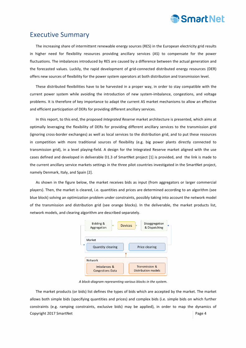
As shown in the figurebelow, themarket receivesbidsas input (fromaggregatorsor larger commercial
players).Then,themarketiscleared,i.e.quantitiesandpricesaredeterminedaccordingtoanalgorithm(see
blueblock)solvinganoptimizationproblemunderconstraints,possiblytakingintoaccountthenetworkmodel
of the transmission and distribution grid (see orange blocks). In the deliverable, the market products list,
networkmodels,andclearingalgorithmaredescribedseparately.
Ablock-diagramrepresentingvariousblocksinthesystem.
Themarketproducts(orbids)listdefinesthetypesofbidswhichareacceptedbythemarket.Themarket
allowsbothsimplebids(specifyingquantitiesandprices)andcomplexbids(i.e.simplebidsonwhichfurther
constraints (e.g. ramping constraints, exclusive bids) may be applied), in order to map the dynamics of
Copyright2017SmartNet Page5
differentflexibilityresourceswhileexpressingtheconstraintsofassets,aggregators,andoperators.Theresult
isacatalogofproductswhichcanbeoptionally integrated in themarket,according to thedesireofsystem
operatorsandregionalregulations.
TransmissionandDistributionnetworkmodelscanbeusedinthemarketclearingalgorithminorder1)to
makesurethattheirconstraintsarenotviolatedwhenclearingthemarket,butalso2)tosolvecongestionor
local problems. There is a trade-off regarding the complexity of the network model to be included in the
constraintsofmarketclearingalgorithm: itcannotbeverysimplified (otherwise itcreatesabigdemandfor
countertrading because the physical constraints of network will not be taken into account in the market
clearing algorithm) but it cannot be too complex (in order to maintain the algorithm computationally
tractable).Therefore,apropernetworkmodel ischosenbasedonthetype,topology,andsizeofthepower
network. The selected model is a second-order cone programming model (SOCP) model for distribution
networkandadirectcurrent(DC)modelforthetransmissionnetwork.
In the clearing module, methods for finding the optimal values of traded quantity (of energy) and the
resulting price (of the corresponding quantity) are developed. The clearings of quantity and price are not
separable tasks,but rather sequentialproceduresbelonging to the samemodule. Themost straightforward
andmeaningfulmethodsofclearingareexplained.
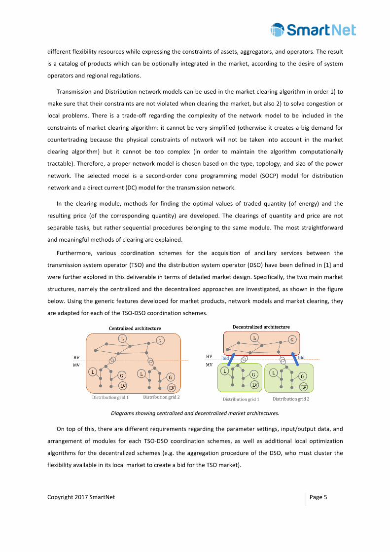
Furthermore, various coordination schemes for the acquisition of ancillary services between the
transmissionsystemoperator(TSO)andthedistributionsystemoperator(DSO)havebeendefinedin[1]and
werefurtherexploredinthisdeliverableintermsofdetailedmarketdesign.Specifically,thetwomainmarket
structures,namelythecentralizedandthedecentralizedapproachesareinvestigated,asshowninthefigure
below.Usingthegenericfeaturesdevelopedformarketproducts,networkmodelsandmarketclearing,they
areadaptedforeachoftheTSO-DSOcoordinationschemes.
Diagramsshowingcentralizedanddecentralizedmarketarchitectures.
Ontopofthis,therearedifferentrequirementsregardingtheparametersettings,input/outputdata,and
arrangement of modules for each TSO-DSO coordination schemes, as well as additional local optimization
algorithms for thedecentralizedschemes (e.g. theaggregationprocedureof theDSO,whomustcluster the
flexibilityavailableinitslocalmarkettocreateabidfortheTSOmarket).
Copyright2017SmartNet Page6
TableofContents
1IntroductionandObjectives...................................................................................................101.1 Context....................................................................................................................................101.2 Objectiveandscope................................................................................................................121.3 DocumentStructure................................................................................................................13
2MarketDesign.........................................................................................................................142.1 BiddingAspects.......................................................................................................................14
2.1.1 FeedbackfromConsultation:Bidding.................................................................................152.2 TimingAspects........................................................................................................................15
2.2.1 FeedbackfromConsultation:Timing..................................................................................182.3 ClearingandPricingAspects...................................................................................................18
2.3.1 FeedbackfromConsultation:ClearingandPricing.............................................................192.4 NetworkAspects.....................................................................................................................20
2.4.1 FeedbackfromConsultation:Network...............................................................................202.5 ProblemStatement.................................................................................................................21
2.5.1 TheGrid...............................................................................................................................212.5.2 TheSystemSteady-StateConditions...................................................................................212.5.3 TheFlexibilityProviders.......................................................................................................222.5.4 TheMarketObjective..........................................................................................................22
2.6 PotentialsofIntegratedReserve.............................................................................................232.6.1 OptionalServiceExpansion:Co-optimizationwithVoltageRegulation..............................232.6.2 OptionalTimingExpansion:FinerTime-ResolutionforFirstTime-Step..............................24
2.7 CoverageofExistingSituationsinOtherRegions....................................................................242.7.1 ExistingMarketinCalifornia...............................................................................................242.7.2 ExistingASMarketsinPilotCountries.................................................................................252.7.3 RequirementsforExtensionofCurrentAS-Markets............................................................27
3BiddingProcessandMarketProducts....................................................................................283.1 Assumptions............................................................................................................................283.2 TypeofBids.............................................................................................................................29
3.2.1 UNIT-bids............................................................................................................................293.2.2 Q-bids..................................................................................................................................313.2.3 Qt-bids.................................................................................................................................313.2.4 QuantityandPriceConventions..........................................................................................313.2.5 PrimitiveBidDefinition.......................................................................................................323.2.6 DecomposingQ-BidsintoPrimitiveBids.............................................................................343.2.7 DefinitionofAcceptance.....................................................................................................35
3.3 CommitmentofMarketDecisions..........................................................................................353.4 Intra-BidTemporalConstraints...............................................................................................36
3.4.1 Accept-All-Time-Steps-or-NoneConstraint.........................................................................363.4.2 RampingConstraints...........................................................................................................373.4.3 MaximumNumberofActivationsConstraint......................................................................383.4.4 MinimumandMaximumDurationofActivationConstraint..............................................383.4.5 MinimalDelayBetweenTwoActivations............................................................................383.4.6 IntegralConstraint..............................................................................................................38
3.5 Inter-BidLogicalConstraints...................................................................................................393.5.1 ImplicationConstraint.........................................................................................................403.5.2 ExclusiveChoiceConstraint.................................................................................................40
Copyright2017SmartNet Page7
3.5.3 DeferabilityConstraint........................................................................................................413.6 IncludingReactivePowerinBids.............................................................................................41
4GridModelforMarketClearing:Trade-OffsinTractability,Accuracy,andNumericalAspects........................................................................................................................................444.1 Introduction............................................................................................................................444.2 ChallengesinOptimalPowerFlow..........................................................................................44
4.2.1 OptimalPowerFlow............................................................................................................444.2.2 ConvexRelaxationApproaches...........................................................................................454.2.3 ConvexRelaxationofOPF...................................................................................................464.2.4 FurtherBackground............................................................................................................48
4.3 ConvexRelaxationFormulations.............................................................................................484.3.1 CompactFormulationofExtendedSOCPBranchFlowModel............................................49
4.4 ImpactofFormulationandRelaxation....................................................................................504.4.1 NumericalStability..............................................................................................................504.4.2 Scaling.................................................................................................................................504.4.3 Variables.............................................................................................................................514.4.4 ConvexificationSlack...........................................................................................................514.4.5 Penalties..............................................................................................................................514.4.6 Objective.............................................................................................................................52
4.5 ApproximatedOPFFormulations............................................................................................524.6 NetworkSimplifications..........................................................................................................53
4.6.1 ExternalGridEquivalent......................................................................................................534.6.2 NetworkReduction.............................................................................................................54
4.7 Summary.................................................................................................................................56
5ClearingAlgorithmandNodalPricing....................................................................................585.1 BalancingObjective.................................................................................................................595.2 TheMarketObjectiveFunction...............................................................................................59
5.2.1 MinimizationofActivationCost..........................................................................................605.2.2 MaximizationofSocialWelfare..........................................................................................615.2.3 MultiTime-StepObjectiveFunction....................................................................................625.2.4 AvoidingUnnecessaryAcceptance......................................................................................63
5.3 NodalPhysicalConstraints......................................................................................................645.4 PricingApproach.....................................................................................................................645.5 NodalMarginalPricing............................................................................................................65
5.5.1 PricingoverSpaceandTime...............................................................................................665.5.2 Granularity..........................................................................................................................66
5.6 CalculatingPrices....................................................................................................................665.6.1 NodalClearedPricesasDualVariables...............................................................................67
5.7 Alternating-CurrentPowerFlow.............................................................................................685.7.1 DistributionLocationalMarginalPricing............................................................................68
5.8 MarketClearingAlgorithm......................................................................................................69
6TSO-DSOCoordinationSchemes............................................................................................706.1 CentralizedvsDecentralizedMarketArchitectures................................................................706.2 MarketSpecificitiesforEachTSO-DSOCoordinationScheme................................................71
6.2.1 CentralizedASMarket.........................................................................................................726.2.2 LocalASMarket..................................................................................................................736.2.3 SharedBalancingResponsibilityModel..............................................................................746.2.4 CommonTSO-DSOASMarket(Centralized)........................................................................75
Copyright2017SmartNet Page8
6.2.5 CommonTSO-DSOASMarket(Decentralized)....................................................................766.2.6 IntegratedFlexibilityMarket...............................................................................................76
6.3 BiddingfromLocalMarketstoCentralMarket.......................................................................776.4 ParametricLocalMarketClearing...........................................................................................776.5 FinancialSettlementandSharingofCostsBetweenTSOAndDSO........................................78
7Conclusions..............................................................................................................................807.1 Bidding....................................................................................................................................807.2 Network...................................................................................................................................807.3 ClearingandPricing.................................................................................................................807.4 CoordinationSchemes............................................................................................................81
8References...............................................................................................................................82
9Appendices..............................................................................................................................889.1 FormulationofBidsandConstraints.......................................................................................88
9.1.1 Nomenclature:ConstantsandVariables.............................................................................889.1.2 StructureofDataforDefinitionofBids...............................................................................909.1.3 DefinitionofAcceptance.....................................................................................................919.1.4 FormulationofConstraints.................................................................................................92
9.2 NetworkModeling..................................................................................................................979.2.1 Nomenclature.....................................................................................................................979.2.2 Notation..............................................................................................................................989.2.3 PhysicsofPowerFlow.........................................................................................................989.2.4 GridElements......................................................................................................................999.2.5 Kirchhoff’sCircuitLaws.......................................................................................................999.2.6 PowerFlow........................................................................................................................1009.2.7 Nodes................................................................................................................................1009.2.8 ClassicPowerFlowFormulations......................................................................................101
9.3 ExtendedOPFFormulation...................................................................................................1059.3.1 Transformer......................................................................................................................1069.3.2 Switch................................................................................................................................1069.3.3 BranchFlowModelFormulation:DistFlow.......................................................................1079.3.4 BusInjectionModelFormulation......................................................................................1119.3.5 QCrelaxation....................................................................................................................1139.3.6 OPFApproximation:LinearDCFormulation.....................................................................1179.3.7 OPFwithAdditionalModels..............................................................................................1209.3.8 Networkmodelingformulationextra’s.............................................................................122
9.4 Illustrationofpowerflowapproximationsandrelaxations:calculationresults...................1239.4.1 Objective...........................................................................................................................1239.4.2 CaseStudies......................................................................................................................1249.4.3 ToolChain.........................................................................................................................1279.4.4 NumericalComparisonofOPFFormulations....................................................................1289.4.5 VerificationStudyoftheInactiveConstraintsMethod.....................................................1389.4.6 VerificationStudyoftheDCApproximationforTransmissionGridModeling..................141
9.5 MathematicalFormulationofMarketClearing.....................................................................1509.5.1 CouplingofPhysicsandEconomics...................................................................................1509.5.2 AdaptationofPricestoAvoidUnnecessaryAcceptance...................................................1509.5.3 NetworkConstraintsforMarketClearing.........................................................................1529.5.4 AnExampleofNodalMarginalPricing.............................................................................1539.5.5 AnExampleofZonalPricing..............................................................................................154

Copyright2017SmartNet Page9
9.5.6 PricinginthePresenceofBinaryVariables.......................................................................1559.5.7 AlgorithmforCalculatingPriceswithPossibleIndeterminacies.......................................1559.5.8 DCversusACon2-nodeExample......................................................................................1569.5.9 ThreeApproachestoPricingwithACPowerFlow............................................................157
Copyright2017SmartNet Page10
1 IntroductionandObjectives
1.1 Context
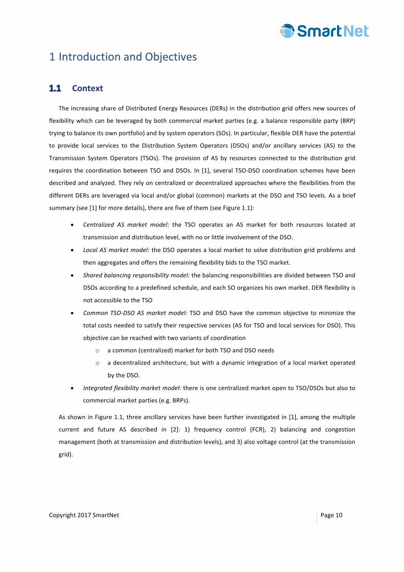
TheincreasingshareofDistributedEnergyResources(DERs)inthedistributiongridoffersnewsourcesof
flexibilitywhichcanbe leveragedbybothcommercialmarketparties (e.g.abalanceresponsibleparty (BRP)
tryingtobalanceitsownportfolio)andbysystemoperators(SOs).Inparticular,flexibleDERhavethepotential
to provide local services to the Distribution System Operators (DSOs) and/or ancillary services (AS) to the
Transmission SystemOperators (TSOs). The provision of AS by resources connected to the distribution grid
requires thecoordinationbetweenTSOandDSOs. In [1], severalTSO-DSOcoordination schemeshavebeen
describedandanalyzed.Theyrelyoncentralizedordecentralizedapproacheswheretheflexibilitiesfromthe
differentDERsareleveragedvia localand/orglobal(common)marketsattheDSOandTSOlevels.Asabrief
summary(see[1]formoredetails),therearefiveofthem(seeFigure1.1):
• Centralized AS market model: the TSO operates an AS market for both resources located at
transmissionanddistributionlevel,withnoorlittleinvolvementoftheDSO.
• LocalASmarketmodel: theDSOoperatesa localmarkettosolvedistributiongridproblemsand
thenaggregatesandofferstheremainingflexibilitybidstotheTSOmarket.
• Sharedbalancingresponsibilitymodel:thebalancingresponsibilitiesaredividedbetweenTSOand
DSOsaccordingtoapredefinedschedule,andeachSOorganizeshisownmarket.DERflexibilityis
notaccessibletotheTSO
• CommonTSO-DSOASmarketmodel: TSOandDSOhave thecommonobjective tominimize the
totalcostsneededtosatisfytheirrespectiveservices(ASforTSOandlocalservicesforDSO).This
objectivecanbereachedwithtwovariantsofcoordination
o acommon(centralized)marketforbothTSOandDSOneeds
o adecentralizedarchitecture,butwithadynamic integrationofa localmarketoperated
bytheDSO.
• Integratedflexibilitymarketmodel:thereisonecentralizedmarketopentoTSO/DSOsbutalsoto
commercialmarketparties(e.g.BRPs).
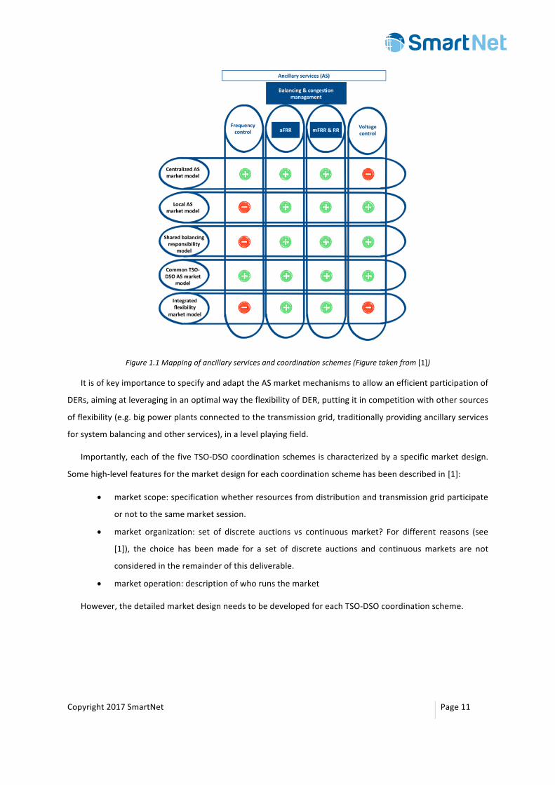
AsshowninFigure1.1,threeancillaryserviceshavebeenfurther investigatedin[1],amongthemultiple
current and future AS described in [2]: 1) frequency control (FCR), 2) balancing and congestion
management(bothattransmissionanddistributionlevels),and3)alsovoltagecontrol(atthetransmission
grid).
Copyright2017SmartNet Page11
Figure1.1Mappingofancillaryservicesandcoordinationschemes(Figuretakenfrom[1])
ItisofkeyimportancetospecifyandadapttheASmarketmechanismstoallowanefficientparticipationof
DERs,aimingatleveraginginanoptimalwaytheflexibilityofDER,puttingitincompetitionwithothersources
offlexibility(e.g.bigpowerplantsconnectedtothetransmissiongrid,traditionallyprovidingancillaryservices
forsystembalancingandotherservices),inalevelplayingfield.
Importantly,eachofthefiveTSO-DSOcoordinationschemesischaracterizedbyaspecificmarketdesign.
Somehigh-levelfeaturesforthemarketdesignforeachcoordinationschemehasbeendescribedin[1]:
• marketscope:specificationwhetherresourcesfromdistributionandtransmissiongridparticipate
ornottothesamemarketsession.
• market organization: set of discrete auctions vs continuousmarket? For different reasons (see
[1]), the choice has beenmade for a set of discrete auctions and continuousmarkets are not
consideredintheremainderofthisdeliverable.
• marketoperation:descriptionofwhorunsthemarket
However,thedetailedmarketdesignneedstobedevelopedforeachTSO-DSOcoordinationscheme.
Copyright2017SmartNet Page12
1.2 Objectiveandscope
The main objective of this deliverable is to further define the AS market design for each TSO-DSO
coordinationscheme,andestablishamathematicalmodelofthemarketclearingalgorithmneededtodefined
thedispatchedquantitiesandpricesoftheASmarket.
Whendesigningaplatformforancillaryservices,twodifferentaspectscanbeconsidered:theprocurement
oftheseancillaryservicesintermsofcapacityandtheactualactivationoftheseservicesintermsofenergy.
WhileactivationofASisbynatureareal-timeprocess,theprocurementofflexibilitycapacitycanbeayearly,
monthly, weekly, daily or even close to real-time. Furthermore, different co-optimization mechanisms
betweencapacityprocurementandactivationofAScanbeconsidered.InthecontextoftheSmartNetproject,
onlytheactivationcomponentisconsidered1:howtodesignareal-timeenergymarketwhereflexibilitiesfrom
DERsandfromassetsconnectedatthetransmissionnetworklevelareactivatedinanoptimalway.
Basedonthischoice,theFCRancillaryservice(seeFigure1.1), isnotfurtherconsideredinthefollowing,
sinceitmakesnosensetohaveareal-timemarketforFCR,sincetheactivationofthisfastfrequencycontrolis
based on local controllers measuring the network frequency, and correcting for any deviation. The same
commentappliestoaFRR,forwhichtheactivationisautomaticandtheupdateofthesetpointstoofrequent
(5-10sec)toallowamarkettodefinetheactivationoftheseproducts.
Also,itwaschosennottoinvestigatethevoltage-controlservice(seeFigure1.1)atthetransmissiongrid,
becauseofthelocalcharacteristicofsuchservice,thatcannotguaranteesufficientmarketliquidity.
Instead, inthisdeliverable,thereal-timeenergymarketdesignisdevelopedtoconsidertheactivationof
balancingandcongestionmanagementservices(forthelatter,bothintransmissionanddistributionancillary
services).Aninnovativemarketdesignisproposed,inorderto:
• leverage flexibilities coming from both transmission grid and distribution grid resources
(geographicalscopeexpansion,comparedtomostcurrentASmarkets,see[1],[2]).
• combinemultipleservices inasinglemarket:providingbalancingservicestothewholesystem,
but also providing congestion management both at the level of distribution and transmission
networks (services scope extension). In particular, this requires to take the transmission and
distributiongridconstraints(ifany)intoaccountinthemarketdesign.
• develop a generic timing extension (timing scope extension), consisting of a higher clearing
frequency(ifneeded)andconsidering(thepossibilityof)arollingtimehorizon(similartowhatis
alreadydoneinCaliforniaforinstance[3]).
1Itisassumedthatthereservehasalreadybeenprocuredand/orthatregulationenforcessomeresourcestoprovideAS.Also,freebidscanalsobeconsideredinthisenergyreal-timemarket.
Copyright2017SmartNet Page13
In this deliverable, this generic market design is called The Integrated Reserve market design. It is
importanttospecifythatwithspecificchoicesofsettingsofthismarket,wecanreproducetheactivationof
existingFRRand/orRRreserves.However,withothersettings, itcanbeamorebenchmarkmodel,perhaps
moreambitious,butstillrealisticinthelongterm.
Thekeychallengeofthisnewmarketdesignistocreateaneconomicallyefficientbutalsocomputationally
tractablemarketclearingprocessfortheIntegratedReservemarket,forthesedifferentTSO-DSOcoordination
schemes,suchthatallpossibleconstraintscanbetakenintoaccount,includingforinstancetransmissionand
distributionnetworkconstraints,aswellasmarketproductsandtheirassociatedconstraints.
1.3 DocumentStructure
This deliverable aims at proposing a generic design for Integrated Reserve market, to be aligned and
adaptedtoeachTSO-DSOcoordinationschemesdevelopedin[1].ThetargetedmarketwillallowTSO/DSOto
leverageflexibilitiesfromDERsinanefficientwayandprovideASbothatthelocalandgloballevel.
InChapter2,wegiveageneraloverviewoftheaspectstobetackledinthemarketdesign.Timing,bidding
andpricingaspectsareaddressed togetherwith thequestionsof thesystemsteady-stateconditionsandof
thenetworkmodeling.Also,optionalextensions (in termsofASandtiming)arediscussed,andwedescribe
how the Integrated market reserve can fit to the current AS market settings in place in the three pilot
countries(Denmark,ItalyandSpain).
InChapter3,wedeepdiveintothebiddingaspects,proposingacatalogueofdifferentmarketproductsto
bidtheflexibilityofDERsinthenewASmarketanddescribingthecorrespondingmathematicalrepresentation
ofthesemarketproducts.
InChapter4,severalmodels(withvaryinglevelofcomplexity)ofthedistributionandtransmissionnetwork
modelareconsidered,andoptimalpowerflowequationsaredescribed.Networkmodelswillbeusedinthe
marketclearingalgorithminordertotakethenetworkconstraintsintoaccount.
InChapter5,wederivethemathematicaloptimizationproblemusedforclearingthemarket.Inparticular,
theacceptanceprocedure,theobjectivefunction,necessarynetworkconstraints,andotherrelatedmaterial
aredescribedindetail,togetherwiththeirmathematicalformulation.Furthermore,weexplainthederivation
of Distributed Locational Marginal Prices (DLMP) using the dual variables of the optimization problem
describedinchapter5andprovideaninterpretationforthesenodalprices.
Finally, Chapter 6 explains how the developed market modules can be used to implement the market
designofthevariousTSO-DSOcoordinationschemesdescribedin[1].

Copyright2017SmartNet Page14
2 MarketDesign
Inthepreviouschapter,weintroducedtheideabehindtheIntegratedReservemarketandexplainedhow
it differentiates from the current solutions for balancing and other ancillary services. In this chapter, we
describe themain aspectsof themarketdesign for the IntegratedReservemarket, namelybidding, timing,
clearing,andnetworkaspects.
2.1 BiddingAspects
TheIntegratedReservemarketisorganizedasaclose-to-real-timemarketforexchangingflexibilities
provided by conventional and renewable resources at transmission and distribution level. Similar to
other energy markets, the traded quantities correspond to electricity injection or off-take. The
flexibilitiesareobtainedbymodifyingtheplannedschedule/commitmentonpreviousmarkets (suchas
day-aheadandintra-daymarkets),orbymodifyingthereal-timebaselineoperation.
Note that, as mentioned in Chapter 1, capacity procurement for the Integrated Reserve is not
consideredintheSmartNetprojectperimeterandthatwefocushereontheactivationdecisionprocess.
The Integrated Reserve market architecture aims at allowing flexible resources coming from both
transmission and distribution networks to compete in the same ancillary services market. In such a
market, what is traded is the service: the sellers are aggregators or sufficiently large flexible assets
connected at transmission or distribution levels; while the buyer is usually a grid operator that in a
centralized architecture usually coincides with the TSO that is active in the control zone, whereas it
couldalsobetheDSOinadecentralizedarchitecture,orevencommercialmarketparties(CMP)inother
proposedcoordinationschemes.
Within a givenmarket session, a flexibility providerwill place a bid in the formof a price-quantity
curve specifying the price asked for different levels of extra supply or consumption of energy (via the
extra injection or off-take of active power). Both positive and negative quantities are, therefore,
consideredtoaccountforupwardanddownwardbalancingenergy.
On top of the economical parameters, a bid on this market includes information on the physical
location of assets: for assets in the distribution grid, to which node of the medium-voltage (MV)
distribution network it is connected, and for assets in the transmission grid, to which node of the
transmissiongrid it isconnected.This locational informationhastobeavailableforthemarketclearing
algorithmtocomputeandlimitthepowerflowsinthenetwork.
If needed by the bidder, a bid on the market can also include some sort of temporal or logical
constraints,forexample:
• Rampingconstraints;
Copyright2017SmartNet Page15
• Maximumnumberofactivationsoveratimehorizon;
• Minimumandmaximumdurationofanactivationrequest(intermsofnumberoftimesteps);
• Minimumdurationbetweentwoactivations;
• andcomplexgenerationbids(e.g.theintegralofenergyinjectionoveragivenperiod).
Adescriptionofbiddingprocessandthedetailedmathematicaldefinitionofthemarketproductsiscarried
outinChapter3.
2.1.1 FeedbackfromConsultation:Bidding
Apublic consultation survey regarding various aspectsofmarketdesignwas carriedoutonline [4] for a
durationof2months.Severalquestionswereaskedand12participatinginstitutes2providedtheirfeedbacks
forthesurvey.Furtherinformationaboutthedistributionofparticipantsisgivenintheappendix.Ingeneral,
the majority of participants believed in a future ancillary service market which is more dynamic, more
extensive,andeconomicallyefficient.
There were 4 questions about bidding aspects of market design, covering topics of allowing complex
products,theresponsiblegridparty,andthetypeofcomplexproducts.
Regardingtheintroductionofcomplexproducts,onlytwoparticipantsopposedthefundamentalidea.Half
oftheanswerssuggestedthatsuchadvancedproducts/bidsmaybeallowed,withtheconcernthat itwould
create a tradeoff between reflecting the market needs, market liquidity, and complexity of computations.
Finally, fourparticipantsapproved the ideaby reasoning that suchproductswill enhance the integrationof
distributedenergyresources(DERs).
Themajorityofparticipantswereleaningtowardstheideathattheaggregator,andnotthemarket,should
handle the dynamic and economic aspects of DER constraints. Only two respondents suggested that the
marketshouldtakecareofsuchconstraints,withoutprovidingastrongargument.
Regarding the list of suggested advanced market products, 5 participants selected products which are
implementedasapartofSmartNetproject.Furthermore,alltheadditionallyrecommendedmarketproducts
(astheanswertoaseparatequestion)werealreadyapartofSmartNetmarketdesign.
2.2 TimingAspects
Somekeyelementsofthemarketdesignliewithintimingaspects.Beforedetailingtheproposal,wefirst
definesometimingnotionsthatwillbeusedextensivelyinthisdocument(asshowninFigure2.1):
2 ACER, Clevergy, Comillas, cyberGRID, EDF, EIMV, ENEL, Epex Spot, European Commission, IBERDROLA, RTE, S&Tconsulting.
Copyright2017SmartNet Page16
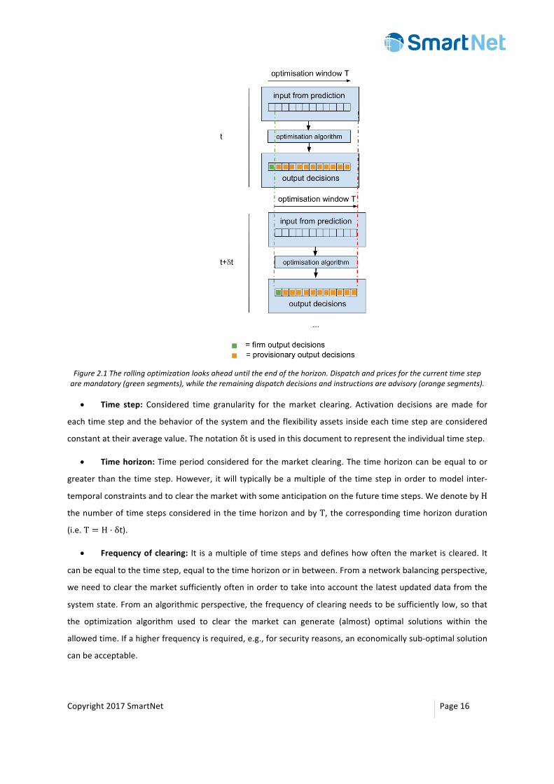
Figure2.1Therollingoptimizationlooksaheaduntiltheendofthehorizon.Dispatchandpricesforthecurrenttimesteparemandatory(greensegments),whiletheremainingdispatchdecisionsandinstructionsareadvisory(orangesegments).
• Time step: Considered time granularity for themarket clearing. Activation decisions aremade for
eachtimestepandthebehaviorofthesystemandtheflexibilityassetsinsideeachtimestepareconsidered
constantattheiraveragevalue.Thenotationδtisusedinthisdocumenttorepresenttheindividualtimestep.
• Timehorizon:Timeperiodconsideredforthemarketclearing.Thetimehorizoncanbeequal toor
greater thanthetimestep.However, itwill typicallybeamultipleof thetimestep inorder tomodel inter-
temporalconstraintsandtoclearthemarketwithsomeanticipationonthefuturetimesteps.WedenotebyH
thenumberoftimestepsconsideredinthetimehorizonandbyT,thecorrespondingtimehorizonduration
(i.e.T = H · δt).
• Frequencyofclearing: It isamultipleof timestepsanddefineshowoftenthemarket iscleared. It
canbeequaltothetimestep,equaltothetimehorizonorinbetween.Fromanetworkbalancingperspective,
weneedtoclearthemarketsufficientlyofteninordertotakeintoaccountthelatestupdateddatafromthe
systemstate.Fromanalgorithmicperspective,thefrequencyofclearingneedstobesufficientlylow,sothat
the optimization algorithm used to clear the market can generate (almost) optimal solutions within the
allowedtime.Ifahigherfrequencyisrequired,e.g.,forsecurityreasons,aneconomicallysub-optimalsolution
canbeacceptable.
Copyright2017SmartNet Page17
• Rollingoptimization:Whenthefrequencyofclearing isshorterthanthetimehorizon,asametime
stepwill typicallybe cleared/optimizedmultiple timeswithupdatedand refined informationon the system
stateandDERavailability.Thisrollingoptimizationallowsthemarketoperatortocombinefrequentclearing,
alwaysusing the latest information and forecasts of system imbalance, and anticipationon the future time
steps.
• TemporalData:Therollingoptimizationuseshistorical,real-time,andforecasteddata.Historicaldata
is used to understand the outcome of previous market (day-ahead, intra-day, etc.) as well as previous
activations of the Integrated Reserve market (up to the current time step). Real-time data includes those
providedtothemarketbyexternalsources(suchasmeasurementsofinjectionsandoff-takesateachnodeof
thenetwork,providedbyTSO/DSO).Thesedataareusedtocalculate/estimatethesteady-stateconditionsof
thesystem,aswellastheinitialconditionsforthebeginningofthenexttimestep.Forecasteddata(suchas
forecastedsystemimbalanceateachnode)arecrucialfortherollingoptimizationtofunction.Forthisproject,
weassumethesedatatobeavailablebeforetheclearingprocessateachtimestepandtheircalculationisnot
discussed.
Using a rolling optimization approach implies that the samemarket time-step can be cleared in several
consecutive optimizations. As the time window moves forward and the state of the system evolves, the
activation decisions can be different for the same time step between two different market clearings. This
raisestheissueofthefirmnessfortheactivationdecisions:
• For the first time-step of the considered time horizon, the activation decisions generated by the
marketclearingarebynaturefirmasitisthelasttimethatthistimestepisconsideredinthemarketclearing.
• For theother times stepsof the considered timehorizon, someof thedecisions couldbe firmand
thereforenotavariableanymoreforthefuturemarketclearingsconsideringthistimestep(e.g.theactivation
of an asset with a constraint of minimum duration of activation) while other market decisions could be
indicativebutnotbinding(e.g.theexactquantityofflexibilityaskedtothisassetfortheconsideredtimestep).
Itisalsoimportanttonotethatifweonlyproposesomevaluesforthelengthoftimestep,timehorizon,
andfrequencyofclearing,buttheyaremodelparametersthatcanbechangedattheimplementationstage.
The parameters clearing frequency and time horizon can be adjusted in the course of the project
activities based on the size/complexity of the considered network, the number and complexity of the
bidsonthemarketandontheperformanceoftheclearingcomputer:
• Theclearing frequency ismainlyacompromisebetweenthedesire todealeffectivelywith the
minute-by-minute fluctuation of renewable resources and the computational burden imposed by the
highcomplexityoftheproblem.
• Asforthedurationofthehorizon,considerthatitcouldbebeneficialtoactivateanassetnow,
butitcouldbealsobeneficialtoactivateitlater.Iftherearenotemporalconstraints,wecouldevendo

Copyright2017SmartNet Page18
both.However, ifwe imaginethatanassetcouldonlybeactivatedonceperhour, themarketneedsto
decidewhethertoactivateitnow,inthenexttimestep,orlateron.Forthis,weneedawindowonthe
futurebeyondthecurrentclearingtimestepandarollingoptimization.Ideally,thehorizonhastobeof
the order of the time duration associatedwith these constraints. Note that in our system, assets can
haveramp-up/downlimitationsormanyothertemporalconstraints.Furthermore,thehorizonshouldbe
selected considering the accuracy limitation of forecasts. This means that if, for example, the latest
“acceptable”forecast isavailableforonehourahead,thehorizonshouldnotbeselectedastwohours.
Vice versa, if the horizon is shorter that the latest acceptable forecast, the potentials of rolling
optimizationwillnotbeharvested.
The Integrated Reserve market relies on the fact that we will be able to simultaneously identify,
discriminate, leverage, commit and dispatch DERs based on their cost but also based on their
operationalconstraints.Inparticular,howfastorslowacertainDERcanreacttoactivationwillhavean
impactonwhetheritisdispatchedornot.
2.2.1 FeedbackfromConsultation:Timing
In this sectionof thesurvey,4questionswereasked.Thequestioncovered the topicsofmore frequent
marketclearing(closertoreal-time),rolling-horizonoptimization,andimbalanceforecasting.
Therewas no opinion against amore frequentmarket clearing,which supported this fundamental idea
implemented in SmartNet as a 5-minute auction market. Furthermore, more than half of the participants
confirmedthat it is feasibletomanagethe inputsandoutputswithin5minutes.Somewereskepticalabout
suchafastclearing-scheme,arguingthatthesystemisnotreadyforthischangeyet,orclaimingthatitwillnot
createanybenefitsforthemarket.Inaverage,theanswersweremoresupportivethanopposing.
Regardingtherolling-horizonoptimization,wereceiveda100%ofpositivefeedback,whichwasveryheart-
warming. However, some participants had concerns about challenges with imbalance forecasting and
transparencyofdecisions.
Thepossibilityofimbalanceforecastingwasanotherquestionedtopic.Theanswersinthistopicweresplit.
Whileafirstgroupbelievedthat it ispossibleandevenalreadyexisting,thesecondgroupdoubtedthat it is
technologicallyfeasibleand/orthatitwillbesoonavailable.Somebelievedthatimbalanceforecastingwillbe
availableforthetransmissiongrid,butnotfordistributionnodes. Ingeneral, itseemslogicaltoassumethat
suchforecastswillbeavailableinnearfutureandthatthemarketwouldbeabletotakeadvantageofthem.
2.3 ClearingandPricingAspects
Theclearingoftheconsideredmarketisdonebytakingintoaccountthenetworkconstraintsbothat
thetransmissionandthedistributionlevels.

Copyright2017SmartNet Page19
Moreprecisely, themarket-clearing algorithmembeds aDC-power flowmodel for the transmission
network and an approximated AC-power flowmodel (convexification of the AC power flow equations)
forthedistributiongridthatincludescomplexvoltagesandpowers.ThesearedetailedinChapter4.
Theinputstotheclearingandpricingalgorithmare:
• Theforecastedinjectionatthedifferentnodesofthenetworkpriortheactivationdecisions(for
thedifferenttimestepsofthetimehorizon),
• Thedifferentavailableflexibilitybidsprovidedonthemarket(forthedifferenttimestepsofthe
timehorizon)andtheircorrespondingconstraints,
• Andthetransmissionanddistributionnetworkmodels.
Then the market optimization decides which bids (and therefore, which flexible assets) to be
activated.
Themarketassociatesaspecificpriceofupwardanddownwardflexibility(e.g.Europerkilowatt)for
each node at the level of transmission or distribution networks, using the approach of distribution
locationalmarginalpricing(DLMP).
2.3.1 FeedbackfromConsultation:ClearingandPricing
Inthissectionofthesurvey,4questionswereasked.Thetopicswerethetypeanddistributionofprices,as
wellas the typeofobjective function tobeused (amaximizationof socialwelfareversusaminimizationof
activationcosts.)
Firstly,participantswereaskedwhethertheythinkthatmarginalpricingorpay-as-bidshouldbethe
methodologyforpricing.Therewasnotasinglevoteinfavorofpay-as-bid,whichwasinfullagreement
with the current implementation in the SmartNet project. Therewere participants which hesitated to
choose,arguingthattheselectionshouldbemadebasedonthenumberofbids,frequencyofclearing,
etc.
Secondly, the feasibility and benefits of nodal pricing was put into 3 questions. The majority of
respondentsconfirmedthatnodalpricescanbe implementedfromatechnologicalpointofview,while
not many of them think that it is economically advantageous. The reasoning behind is that further
analyses shouldbe carriedoutbeforeopting toonemethodoranother.Also,mostof theparticipants
believethatnodalpricingisacceptablefromaregulatorypointofview.
Finally, regarding the objective function, the majority of participants believe that maximization of
socialwelfare has to be used. This is justifiable from several points of view, including system security,
operationalandinvestmentscosts,etc.However,oneparticipantarguedthatitwill increasethecostof
balancing. In general, we believe that the best objective function to be used is a combination of two

Copyright2017SmartNet Page20
approaches.
2.4 NetworkAspects
Theclearingoftheconsideredmarketwillbebasedonanappropriatemathematicalrepresentationofthe
transmissionanddistributiongrids.Thechallengeistofindanetworkmodelwhichisatthesametime:
• Sufficiently accurate, to identify and solve the balancing and congestion issues and avoid creating
voltageproblems;
• Sufficientlyefficient,tobetractableintheoptimizationproblemwhichissolvedateverytimestep;
and
• Sufficientlysimple,toincludeonlyfunctionsthatareimportanttobuildupthemarketalgorithmand
thetestcases.
The considered approach is to represent the transmission grid with a DC power flow model and the
distributiongridwiththesecond-ordercone(SOC)relaxationoftheACpowerflowmodel.
Asaconsequence,linearconstraintsandSOCconstraintswillbeincludedintheoptimizationproblem.The
detailedequationsofboththetransmissionandthedistributionnetworkwillbepresentedinChapter4ofthis
document.
2.4.1 FeedbackfromConsultation:Network
Inthissectionofthesurvey,5questionswereasked.
First, thegeneralopinionabout the integrationof transmissionanddistributiongrids in themarketwas
questioned.Wereceivedequalnumbersofpositiveandnegativeopinions,withsomeneutralfeedbacks.The
optimistic participants believed that thesemodels can be added gradually, while the pessimistic reviewers
arguedthat itwould introducecomplexitiesandthatweshouldtakethenetworkmodelsoutofthemarket
clearingproblem.
The next 4 questions concerned the availability of data for building the model and for providing
informationonnodalinjectionattransmissionanddistributionlevels.Wereceivedmixedanswers:Ontheone
hand,someparticipantsbelievedthattherequireddataisavailable(atleastfortheTSO)inordertomakethe
modelsandthatinjectionforecastsarepossible.Ontheotherhand,wehaveparticipantswhichbelievedthat
such model data or forecast are difficult to collect and that it is not possible to ask for such data. One
participantclaimedthatimbalanceforecastsarenotevenneeded.Ingeneral,ourtakefromthesequestionsis
thatthepossibilityofhavingaccesstosuchdataishigh,butweshouldalsoconsiderscenarioswhentheyare
notavailable.
Copyright2017SmartNet Page21
2.5 ProblemStatement
As already discussed before, the market we aim to design is a real-time market for activation of
flexibilityresources,connectedbothattransmissionanddistribution levels.Wenowdescribetheexact
optimizationproblemtobesolvedmoreindetail.
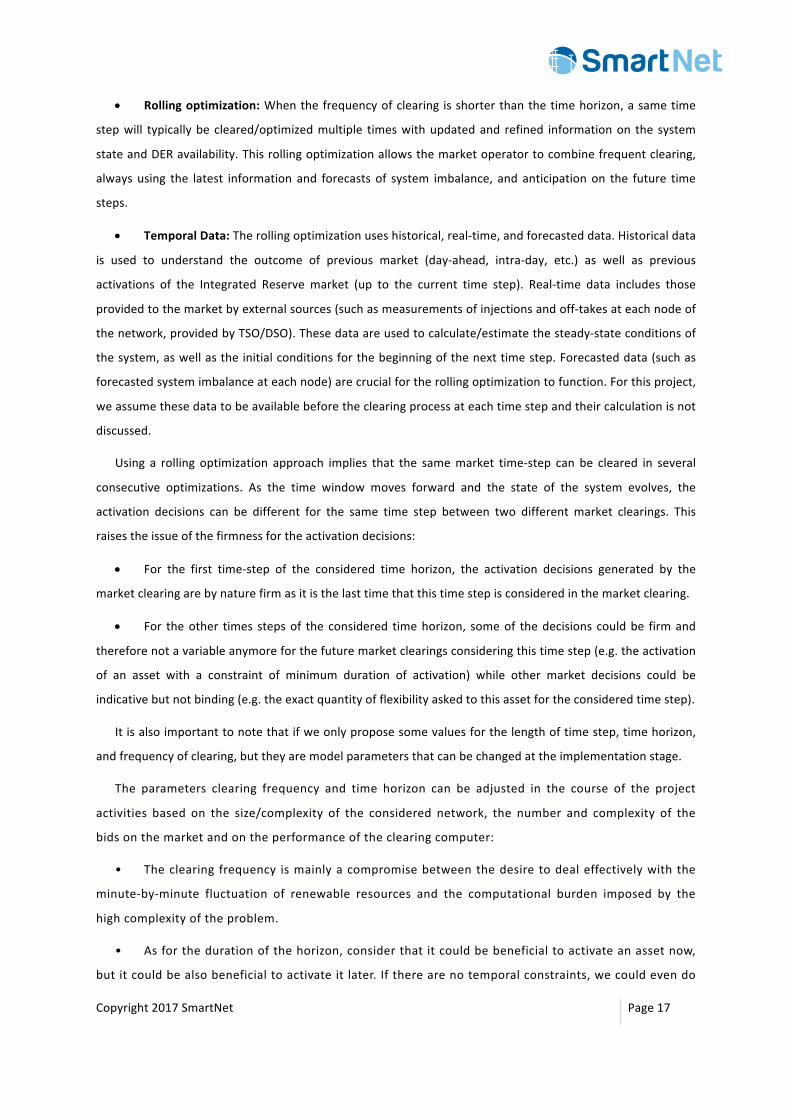
2.5.1 TheGrid
Akeyelementof theproblemstatement is the consideredgrid,which consistsofone transmission
grid anddifferent distribution grids connected to the transmission grid. Thenetwork topology is a key
inputfortheproblemstatement.
Figure2.2Exampleofagridwiththreedistributionnetworks(blue)connectedtothetransmissionnetwork(orange).
2.5.2 TheSystemSteady-StateConditions
Foragiventime-step,anotherimportantelementfortheproblemstatementisthesteady-statesituation
of the system i.e. what would be its state during and at the end of the time step in the absence of any
flexibilityactivationby themarket.The informationregarding thesteady-stateconditions isprovided to the
market by the network operators. It is natural that the complexity of calculation and the accuracy of such
information will be impacted by increasing the clearing frequency of the market. As a result, the clearing
frequencyasa“designparameter”hastobechosenconsideringsuchlimitations3.
Thissteady-statesituationisdefinedbyalltheactiveandreactivepowerinjectionsatthedifferentnodes
ofthenetwork(bothtransmissionanddistribution)resulting:
• frompreviousenergymarkets(e.g.day-aheadorintraday),
3Bysteady-statesituation,wedonotmeanthecurrentsituationofthesystembutwhatwouldbethesituationofthe
systemifnoactivationsweredoneinthemarket.
4 1
2
3
11
12
13
21
22
233
1
32
DSO1
DSO2
DSO3

Copyright2017SmartNet Page22
• from theactivationbyTSOand/orDSOofout-of-marketancillary services (e.g. voltage regulation),
and
• fromdeviations(forecasterrors,unpredictableevents)fromtheseprevioustimeframes.
Itisimportanttonotethatthesesteady-stateconditionsareexpressedatthelevelofeachnetworknode
butnotattheresource level.The injectionsateachnodearethemselvesthecombinationsofthe individual
behaviorofmanydifferentconsumersorproducersofelectricity,butitisnotneededfortheflexibilitymarket
toknowtheseindividualbehaviorsandtomodeltheindividualsourcesofimbalances.
Itisexpectedthatthesesteady-stateconditionsaresuchthat:
• Thereisapowerimbalancebetweensupplyanddemand,
• There are potentially some instances of congestion problems at the lines of the considered
(distributionandtransmission)grids,andthat
• Therearenopre-existingvoltageproblems,asthecorrespondingancillaryserviceshavealreadybeen
activatedpriortothemarket.
2.5.3 TheFlexibilityProviders
ThedifferentDERsandtransmission-networkconnectedassetscanproposetheirflexibilitiestotheTSOat
thenodelevel,eitherasanindividualassetorinanaggregatedway.Byflexibilitywemeanthepossibilityto
changetheactivepowerinjectionatagivennodeofthenetwork.Evenifreactivepowerisnottradeditself,
theimpactofactivationintermsofmodificationofinjectedreactivepowerhasalsotobeincludedinflexibility
bids(forexampleviaapowerfactororarelationbetweenactiveandreactivepower).
Byactivatingdifferentflexibilitybids,theTSOwillmodifythesituationofthenetworkwiththeobjectiveto
solveefficientlytheimbalanceandcongestionproblemsfacedbythenetworkinitssteady-stateconditions.
2.5.4 TheMarketObjective
Inthecomingchapters,wewilldemonstrateamathematicalformulationofthemarketclearingalgorithm,
includingtheobjectivesandconstraints.Atthispoint,itispossibletodiscussthehigh-levelobjectivesofthe
IntegrateReservemarketaslistedbelow.
Given:
• theconsideredgridmodel,
• thesteady-statesituationofthegrid,and
• thedifferentbidsfromflexibilityprovidersateachnodeofthegrid,
theobjectiveofthemarketoperatoristooptimizethechoiceofbidsactivationsinorder
Copyright2017SmartNet Page23
• tosolvetheimbalanceproblematlocalorgloballevel,
• tosolvethepossiblecongestionproblemsintransmissionanddistributionnetworks(orboth),
• nottocreatenewvoltageproblems,
• andtomaximizethesocialwelfareorminimizethecostofactivations(thesewillbeimplementedintheformofanobjectivefunction).
2.6 PotentialsofIntegratedReserve
In thissection,wedescribeacoupleofoptionalbroadenings in themarketdesignwhichcanextendthe
functionalitiesoftheIntegratedReservemarket,allowingittofitintovariousapplications.
2.6.1 OptionalServiceExpansion:Co-optimizationwithVoltageRegulation
TheIntegratedReservemarketisfocusingonbalancingandcongestionmanagementbutincludesvoltage
constraintsandreactivepowerinformationofdistributionnetworks.Thisallowsthemarkettoensurethatthe
activationintermsofactivepower,(madeinordertobalancethesystemandmanagethecongestion)does
notcreatenewproblemsintermsofreactivepowerandvoltage.
However,itisnotexpectedfromthemarkettostartfromasituationwithimportantvoltageproblemsand
tosolvethem,togetherwithbalancingandcongestionmanagement.Inparticular,ifforeachbid,thereactive
power impact of an active power activation is taken into account (via a simple power factor), the reactive
powerisseenasaside-productandnotsomethingwhichistradedonthemarket.Themarketisnotexpected
to “play” with reactive power and to leverage by itself the flexibility in the P/Q ratio of some assets. The
marketproductsarenotdesignedintermsofreactivepower.Thislimitationisjustifiedbythefactthat,while
the resources providing balancing and congestion management are typically the same, voltage regulation
impliestointegrateinthemarketothertypeofassets(e.g.assetsofferingpurereactivepowerflexibility)and
todefineothertypeofproducts(e.g.productsmodelingtheflexibilityintheP/Qratioofsomeassets).
However,asthenetworkmodelusedintheclearingmechanismtakesintoaccountthevoltageconstraints
anyway,itcouldbetemptingtoextendthescopeoftheIntegratedReservetoincludealsovoltageregulation
intheancillaryservicesitcanprovide.Buttodoso,asexplainedearlier,marketproductsshouldberedefined,
suchthatboththeirflexibilities inactiveandreactivepower, ifany,are leveraged.Somebidscouldevenbe
justpurereactivepowerbids.
Fromaneconomicalperspective,providingalltheancillaryservicestogetherinthesamemarketcouldof
course increase theeconomicefficiencyof theancillaryservicesdecisionsbutat thepriceofmorecomplex
market products and clearing mechanism and of stronger deviation from current organization of ancillary
services.
Copyright2017SmartNet Page24
2.6.2 OptionalTimingExpansion:FinerTime-ResolutionforFirstTime-Step
A flexibility provider will bid a price-quantity curve over the decision period of and potentially, for all
decisionperiodsoverthegiventimehorizon.
Arefinementofthisapproach istoconsider, forthefirststepoftherollingoptimization, inputdataata
shortertimeperiodthanthedecisiontimestep(e.g.a1-minuteinputdatatimestepanda5-minutedecision
timestep).Hence,wecan:
• differentiateproductswith the sameaveragepowerover thedecision time stepbutwithdifferent
andirregularpowerprofilesattheinputdatastep(typicallydifferenttypesofreactivity),and
• ensure that the imbalance is correctlymatched on the input data time step, which is shorter
thanthedecisiontimestep.
Thisallowstoreducetheneedformorereactivereserve,likeaFRR,astheactivationdecisionmadebythe
IntegratedReserveallowsnotonlytobalancethesystemforeachtimestepbutalsoinsideeachtimestep.
However,pleasenotethatinthisrefinedapproach,wedonotchangethemarketclearingfrequency(e.g.
still5minutes).Therefore,evenwith30seconds inputdata timestep, IntegratedReservecannotprovidea
response timeof 30 seconds at any time (once themarket is cleared, thenext clearinghappens5minutes
later).Forthisreason,theIntegratedReservecannotreplaceaFRR,whichisstillneededtoreacttounplanned
eventshappeningbetweentwoclearingeventsoftheIntegratedReserve.
2.7 CoverageofExistingSituationsinOtherRegions
Existing ASmarkets general characteristics have been described for 8 European countries in deliverable
D1.1 of the SmartNet project [2]. Since the scope of the Integrated Reserve market is mainly about the
mFRR/RRreserve,thefocusofthissectionisonthesetypesofmarketsinthethreepilotcountries:Denmark
(area DK1), Italy and Spain. In addition, the already existing advanced real-time market in California is
discussedforcomparison.
2.7.1 ExistingMarketinCalifornia
Forthesakeoftheexampleandcomparison,webrieflydescribeoneofthemostadvancedmarketsthat
arealreadyinoperation,featuringhighclearingfrequencyandarollingwindowoperation.Forthisreason,we
alsolistCalifornia[3].ERCOTinTexasrunsasimilaradvancedmarket.
FocusingontheReal-TimeEconomicDispatch(RTED)process inCalifornia,wenoticethat ithasarolling
timehorizonofupto13time-steps(of5-minuteduration),startingexecutionevery5minutesatthemiddleof
the5-minute timesteps (1.5 timestepsbefore thedispatch).TheRTEDstartsatapproximately7.5minutes
(1.5 time steps) prior to the start of the next dispatch interval and produces an instruction for energy
Copyright2017SmartNet Page25
injection/off-take for thenext dispatch interval and advisory dispatch instructions for asmany as 12 future
dispatchintervalsovertheRTEDoptimizationtimehorizon.
Thismeansthatthankstothispipeliningofinputdataanddecisionmaking,1)thedecisiontimestepcan
bechosenshorterthantheneededworstcaselatencyoftheclearingalgorithm,and2)theoldestinputdata
usedwill thenbeone timestepolder thanwithoutusing this trick.Basedon the feedbackof theSmartNet
simulation platform, this pipelining trick could be considered in the design of SmartNet clearing algorithm,
depending on the decision time steps chosen for the simulations and depending on the market clearing
algorithmperformance.Usingthispipelinefeature,atrade-offmustbemadebetweenthebenefitsoftaking
morefeaturesintoaccount(largernetworks,additionalconstraintsorcostfunctionterms)versusthebenefits
ofusingmorerecentinputdata.
AfurtheraspectoftheCaliforniaRTEDmarketisthatbidsarelimitedtomaximum10segmentsalongthe
quantityaxis.Interestingly,bidsspecifyingbothpositiveandnegativequantitiesareallowed.Non-curtailable
blocksarealsoallowed.Forabidassociatedtoagenerator,minimumandmaximumenergyspecifiedinabid
areonlylimitedtowhatthegeneratorcanprovide.
2.7.2 ExistingASMarketsinPilotCountries
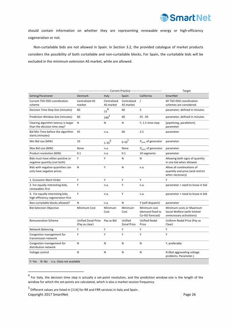
Table2.1describesdetailedmarketsettingsparameters, thatare representative in thecurrentmFRRAS
marketsofthesecountries,andalsosomecomparisonwithaCaliforniareal-timedispatchmarket.
Thisisnecessaryfortworeasons.First,toensurethat,eventhoughwearetryingtoextendthepossibilities
ofexistingenergymarketoperations,wedonotlosesomecapabilitiesandflexibilitiesofcurrentmarkets(last
column of Table 2.1 explains that these settingswill be considered in the description of themore general
Integrated reserve market). Second, to state the ground and then determine the minimum extensions
requiredforthesemarketstobeabletoleveragetheflexibilityoftheDERinthedistributionnetworks(e.g.for
instance,inItaly,DERarenotallowedyettobidontheASmarkets),andrepresentassuchaminimumchange
ASmarketvariant.Decisiontimestepsare60minutesforeachpilotcountry,andnolargerpredictionwindow
is considered.Most countries specifyminimum (max) bid sizes to participate to themarket, aswell as bid
resolution.
InItalyandSpain,bidsareformulatedaseitherbeingupward(only)ordownward(only).So,enforcingthis
as the only allowed bid formulations in the applicable regions has to be catered for in SmartNet. In other
regions,bidswithbothpositiveandnegativeselectablequantitiesshouldbeallowed.
In the three pilot countries, economicmerit order (on price) is the first criterion for bid acceptance. In
Denmark, Spain and Italy, for twobidswith equalmerit order, the renewable energy bids have preference
overtheotherone(althoughforItaly,itappliestoenergymarkets:DA,ID.RESandDERcannotyetbidonAS
markets). Also, when there is no preference between two bids even after the renewability criteria, a bid
representing high efficiency cogeneration is preferred over the other bids. This means that SmartNet bids
Copyright2017SmartNet Page26
should contain information on whether they are representing renewable energy or high-efficiency
cogenerationornot.
Non-curtailablebidsarenotallowed inSpain. InSection3.2, theprovidedcatalogueofmarketproducts
considersthepossibilityofbothcurtailableandnon-curtailableblocks,ForSpain,thecurtailablebidswillbe
excludedintheminimumextensionASmarket,whileareallowed.
4 For Italy, thedecision time step is actually a set-point resolution, and thepredictionwindow-size is the lengthof thewindowforwhichtheset-pointsarecalculated,whichisalsoamarketsessionfrequency.
5Differentvaluesarelistedin[114]forRRandFRRservicesinItalyandSpain.
--------------------------------CurrentPractice-------------------------------- Target
Setting/Parameter Denmark Italy Spain California SmartNet
CurrentTSO-DSOcoordinationscheme
CentralizedASmarket
CentralizedASmarket
CentralizedASmarket
/ AllTSO-DSOcoordinationschemesareconsidered.
DecisionTimeStepSize(minutes) 60 154 60 5 parameter,definedinminutes
PredictionWindowSize(minutes) 60 2404 60 55-65 parameter,definedinminutes
Clearingalgorithmlatencyislargerthanthedecisiontimestep?
N N N Y,1.5time-step [pipelining,parallelism]parameter
BidMinTimebeforethealgorithmstarts(minutes)
45 n.a. 60 2.5 parameter
MinBidsize(MW) 10 1-105 0-105 𝑃()* ofgenerator parameter
MaxBidsize(MW) None n.a. None 𝑃(+, ofgenerator parameter
Productresolution(MW) 0.1 n.a. 0.1 10segments parameter
Bidsmusthaveeitherpositiveornegativequantity(notboth)
Y Y N N Allowingbothsignsofquantityinonebidwhenallowed.
Bidswithnegativequantitiescanonlyhavenegativeprices
N Y N n.a. Allowallcombinationsofquantityandprice(andrestrictwhennecessary)
1.EconomicMeritOrder Y Y Y Y Y
2.Forequallyinterestingbids,renewablesfirst
Y n.a. Y n.a. parameter+needtoknowinbid
3.Forequallyinterestingbids,high-efficiencycogenerationfirst
Y n.a. Y n.a. parameter+needtoknowinbid
Non-curtailableblocksallowed? N n.a. N Y(self-dispatch) parameter
Bid-SelectionObjective MinimumCost MinimumCost
MinimumCost
Minimumcost(demandfixedtoCa-ISOforecast)
MinimumcostsorMaximumSocialWelfare(withlimitedunnecessaryactivations)
RemunerationScheme UnifiedZonalPrice(Payasclear)
PayasBid UnifiedZonalPrice
UnifiedNodalPrice
UniformNodalPrice(PayasClear)
NetworkBalancing Y Y Y Y Y
Congestionmanagementfortransmissionnetwork
Y Y Y Y Y
Congestionmanagementfordistributionnetwork
N N N N Y,preferably
Voltagecontrol N N N N N(Notaggravatingvoltageproblems.Parameter.)
Y:YesN:Non.a.:Datanotavailable
Copyright2017SmartNet Page27
Table2.1Comparisonofmarketsinthethreepilotcountries,CaliforniamarketandwhatisplannedintheframeworkofSmartNetintegratedreserve.
Inallthreepilotcountries,theobjectivefunctionofthemarketclearingalgorithmistominimizeactivation
costs. The remuneration scheme in Italy is of the pay-as-bid-type. Other regions (Denmark and Spain) are
remuneratingaccordingtoauniformmarginalpricescheme.
CurrentancillaryservicesinEuropeancountriesaremainlybalancingandcongestionmanagementonthe
transmissionnetwork.SmartNetwantstotakethisonestepfurthertoalso includecongestionmanagement
fordistributionnetworks.Ontopof that,makingsure thatvoltageproblemsarenotcreatedby themarket
clearingoutputwillbeconsideredaswell.
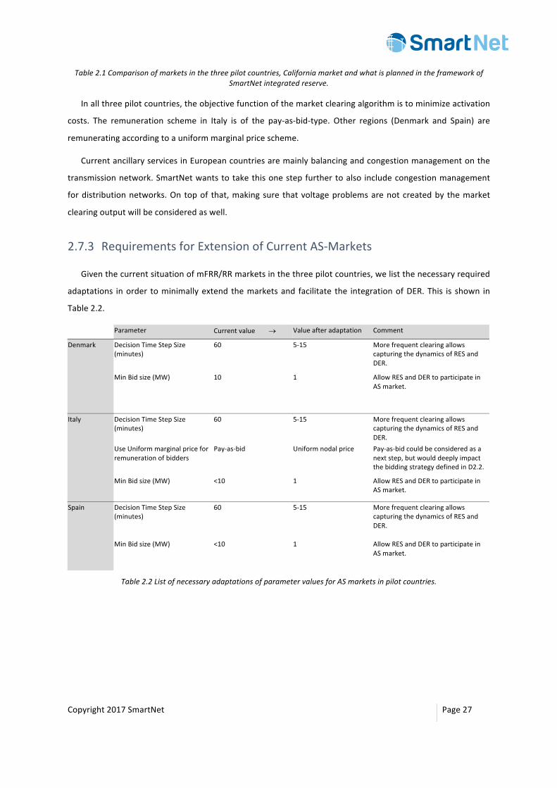
2.7.3 RequirementsforExtensionofCurrentAS-Markets
GiventhecurrentsituationofmFRR/RRmarketsinthethreepilotcountries,welistthenecessaryrequired
adaptations inorder tominimallyextend themarketsand facilitate the integrationofDER.This is shown in
Table2.2.
Parameter Currentvalue® Valueafteradaptation Comment
Denmark DecisionTimeStepSize(minutes)
60 5-15 MorefrequentclearingallowscapturingthedynamicsofRESandDER.
MinBidsize(MW) 10 1 AllowRESandDERtoparticipateinASmarket.
Italy DecisionTimeStepSize(minutes)
60 5-15 MorefrequentclearingallowscapturingthedynamicsofRESandDER.
UseUniformmarginalpriceforremunerationofbidders
Pay-as-bid Uniformnodalprice Pay-as-bidcouldbeconsideredasanextstep,butwoulddeeplyimpactthebiddingstrategydefinedinD2.2.
MinBidsize(MW) <10 1 AllowRESandDERtoparticipateinASmarket.
Spain DecisionTimeStepSize(minutes)
60 5-15 MorefrequentclearingallowscapturingthedynamicsofRESandDER.
MinBidsize(MW) <10 1 AllowRESandDERtoparticipateinASmarket.
Table2.2ListofnecessaryadaptationsofparametervaluesforASmarketsinpilotcountries.

Copyright2017SmartNet Page28
3 BiddingProcessandMarketProducts
The Integrated Reserve market is a market for ancillary services aiming to leverage the flexibility from
assetslocatedbothatthedistributionandthetransmissiongridlevels.Themaingoalofthismarketistosolve
imbalances between energy supply and demand in near real time. A side goal is congestionmanagement,
although it ispossiblethatbalancingandcongestionaredealtwith indifferentmarkets.Flexibilityproviders
bidonthemarketusingthemarketproductsthatareproposed.Themarketoperatorselectsbidsbyrunning
analgorithm,calledthe(market)clearingalgorithm.
While this deliverable takes care of defining the market products and the functionality to clear the
IntegratedReservemarketandtoprice theactivated flexibility in themostefficientway,deliverable2.3 [5]
takescareofaggregatingtheflexibilityofalargeportfolioofDERsandofofferingthisflexibilityonthemarket
usingtheproposedmarketproducts.
Thedefinitionofthemarketproductsisthereforeakeyelementforanefficientcoordinationbetweenthe
aggregatorsandthemarketoperator:
Figure3.1Coordinationbetweentheenduser,theaggregator,andthemarket.
3.1 Assumptions
Thefollowingassumptionsaretakenintoaccountintherestofthischapter:
1. The Integrated Reserve is a discrete/closed-gate market, cleared very frequently (e.g. every 5
minutes)andusingarollingoptimization(e.g.1hour)totakeadvantageofforecasts.
2. A bid can be associated to a specific physical asset (e.g. a large power plant connected to the
transmissiongrid)ortoanaggregatedportfolioofDER.
3. Abid is associated to a specific nodeof the distributionor transmission grid.Multiple bids canbe
presentedatasamenodebymultiplemarketparticipantsbut thesamebidcannotcover resourcescoming
fromdifferentnodesofthenetwork.
4. Amarketparticipantcansubmitbidsfordifferentnodes.
5. A market participant can submit multiple bids for the same node but by default these bids are
considered completely independent. The market can accept all of them, some of them or none of them
Copyright2017SmartNet Page29
without linking constraints. If twobidsof the same issuer are intended tobeexclusively accepted, thenan
exclusive-choiceconstraintwillhavetobeconstructed.
6. The bids are expressed in terms of active power injection/offtake but, associatedwith it, a power
factorwillalsobeprovidedbytheflexibilityproviders.Thisallowsthemarketoperatortomodeltheimpacton
the reactive power side of the different activation decisions, which means that the reactive power is
accountedforinthemodel.Iftheresourcehastheflexibilityforthereactivepower,itcansubmitseveralbids
with the sameactivepowerbutdifferent reactivepowers.Then, theclearingalgorithmwill select themost
suitable bidof this asset. It is important to remember that the goal of IntegratedReservemarket is not to
optimizethereactivepowerflows,buttoavoidcreatingadditionalproblemsrelatedtothat(suchasvoltage
problems).
3.2 TypeofBids
Threemaintypesofbidswithrespecttotheirdimensionaredefined,namelytheUNIT-bid,theQ-bid,andthe
Qt-bid.Eachofthesetypescanbecurtailableornon-curtailable.Acurtailablebidallowsthemarkettoselect
andactivateanyportionofitsquantity(thatisthepowervolume),whileincontraryanon-curtailablebidcan
either be accepted at the given quantity or be rejected. In the rest of this section, each type of the bid is
described.
3.2.1 UNIT-bids
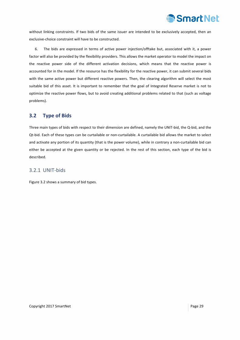
Figure3.2showsasummaryofbidtypes.
Copyright2017SmartNet Page30
Figure3.2Differenttypesofstandardbids(shownonlyfor𝒑, 𝒒 > 𝟎).Standardbidsonlymentionpriceandquantityand
formthe(mandatory)basisofanybid.Threefamiliesofbidsareconsidered:Unit-bids,Q-bids,andQt-bids.
AUNIT-bidisdefinedforaspecifictimestepandissimplydefinedbyapriceandaquantity,asshownin
thefirstrowofFigure3.2.Threesub-typesofUNIT-bidsareconsidered:
1. Non-curtailableUNIT-bid: Thevery simplestbid (seecolumn1ofFigure3.2)hasoneprice forone
quantity,meaningthatthemarketoperatorcaneitheracceptorrejectthetotalenergyquantity𝑄3ataprice
of𝑃3orhigher.Thismarketproductiscallednon-curtailablebecauseeitherthetotalblockhastobeaccepted
or theblock isnotacceptedatall. Themarketcannotaccepta fractionalpartother than0%or100%of it.
Priceandquantitycanbenegativeorpositive.Positivequantitiesstandforenergyinjectionsintothenetwork
andnegativequantities forenergyofftake fromthenetwork.Amarketparticipantcouldsend twoseparate
bids,oneofferinganenergyinjectiontothenetworknodeandanotheroneofferinganenergyofftakefrom
thenetworknode.
2. STEP curtailable UNIT-bid: This UNIT-bid has a single price 𝑃3 = 𝑃4 for a range between two
quantities𝑄3and𝑄4 (seethecolumn2ofFigure3.2).Here,themarketoperatorcanacceptanyquantity in
between𝑄3and𝑄4foratleastthemarginalcostof𝑃3 = 𝑃4(expressedinEUR/MW6).
PWL (piecewise linear) curtailableUNIT-bid: ThisUNIT-bidhas a changingmarginal price𝑃3 to𝑃4 for a
rangebetweentwoMWquantities𝑄3and𝑄4(seethecolumn3ofFigure3.2).Here,themarketoperatorcan
accept any quantity in between 𝑄3 and 𝑄4 for at least the marginal cost on the 𝑃3-𝑃4-line. Detailed
specificationofUNIT-bidsisprovidedintheappendixinSection9.1.2.1.6 Thequantities inMWrepresent theaverageactivepower injection,definedas the ratioof the integralof thepowerprofile/trajectorytotheactivationtimestep(e.g.5minutes).AllthequantityandpriceareexpressedinMWandEUR/MWbutcanbeconvertedinMWhandEUR/MWhusingthefixedtimestepofthemarket.

Copyright2017SmartNet Page31
3.2.2 Q-bids
Q-bidsaresimilartoUNIT-bids,butcanprovidelongervectorsofQandPalongtheQ-axis,asshowninthe
secondrowofFigure3.2.TheobjectiveofaQ-bidistoallowtheCMPtodirectlyexpressanaggregatedcurve
offlexibilitywithvaryingmarginalcost.
SimilartoUNIT-bids,theQ-bidscanbeeithernon-curtailable,stepcurtailableorpiece-wisecurtailableand
theyareassociatedtoaspecifictimestepofthemarketclearing.Also,thepowerfactorisconstantpertime
step,i.e.perQ-bid.DetailedspecificationofQ-bidsisprovidedintheappendixinSection9.1.2.2.
3.2.3 Qt-bids
TheUNIT-bids andQ-bids are associated to a specific time-step and do not allow offering flexibility for
consecutivetimesteps,whichmeansthatthetime-dimensionismissing.
Qt-bids essentially offer aQ-bid for a series of time stepswithin thewindowof optimization and allow
expressinginadvancetheavailabilityofflexibilityforthefuturetimesteps,asdemonstratedinthethirdrow
ofFigure3.2.
Theywill alsobe servingas the standardbidonwhichadditional temporal constraints canbeadded. In
addition, Qt-bids can have a different power factor at each time step. Detailed specification of Q-bids is
providedintheappendixinSection9.1.2.2.
Thenumberofdecision time steps inaQt-bid is called thebid-horizon7. If aQt-bidhasa largerhorizon
thanthetimewindowhorizonconsideredbytheclearingalgorithm,therearetwooptionsforthemarket.The
firstoptionisthatthebidwillnotbeconsideredandthebidderwillbenotifiedofit.Inthiscase,thebidders
arediscouragedtosubmitbidswhichgobeyondthemarkethorizonandtheclearingalgorithmissparedfrom
unnecessarylongbids.Thesecondoptionistocutsuchbidsaccordingtothemarkethorizon.Forexample,if
thehorizonconsistsof12timestepsandaQt-bidcontains13timesteps,themarketconsiderstheQ-bids1to
12forthecurrentmarketclearingandtheQ-bids2to13forthenextmarketclearing. Inthiscase, longbut
feasiblebidsarenotrejected.
3.2.4 QuantityandPriceConventions
In thisdocument,weavoidusing the termsbuyersandsellers.Thereason is that inamarketwithboth
positiveandnegativevaluesforpricesandquantities,thisterminologytendstobeconfusing,sincetheycanbe
definedbasedon thepriceoron thequantity. In this context, a helpful convention is todefine the flowof
things(powerquantitiesinMWorMWh/time-step,andrespectivepricesinEURO/MW)asfollowing:
7Therefore,onecanconsidertheQ-bidasaQt-bidwithonlyonetime-interval(orabidhorizonofone),andsimilarlytheUNIT-bidasaQ-bidwithonlyonequantity-interval.

Copyright2017SmartNet Page32
𝑝 > 0:Thebidderwantstoreceivemoney.
𝑝 < 0:Thebidderwantstopaymoney.
𝑞 > 0:Thebidderinjectsmoreoroff-takeslessenergy(upwardsflexibility).
𝑞 < 0:Thebidderoff-takesmoreorinjectslessenergy(downwardsflexibility).
Ifastandardsupply-demandmarketwouldusethisconvention,ageneratorwouldusuallysubmitbidswith
𝑝, 𝑞 > 0andaconsumerwouldusuallysubmitabidwith𝑝, 𝑞 < 0.However,evenintheEuropeanday-ahead
electricitymarket,bothpositiveandnegativevaluesof𝑝areacceptable8.
Insomelesscommonmarkets,allfourpossiblecombinationsof𝑝and𝑞canappearinbids.Asanexample,
an hour of high wind may cause the network to contain more energy than predicted. In such a scenario,
removingtheextraenergyisconsideredtohaveapositivecontributiontowelfare.Therefore,generatorswill
beintheunusualpositionofbiddingapositive𝑞(injectingenergy)withanegative𝑝(payingmoney).Similarly,
energyconsumerscansubmitbidswithanegative𝑞(off-takingenergy)withapositive𝑝(receivingmoney).
In the IntegratedReservemarket,weare interested in theassetsproviding flexibility inbothdirections.
Therefore, it is not the absolute supply and demand, but the relative increase/reduction in generation or
consumptionthatisimportant.Asanexample,ageneratorreducingitsgenerationlevelisprovidingthesame
typeofflexibilityasaconsumerincreasingitsconsumptiondoes.Theseassetswillbothsubmitbidswithq < 0
and are considered as downwards flexibility. Vice versa, an increase in generation or a decrease in
consumptionisregardedasupwardsflexibilityandisrepresentedwithq > 0bids.Therefore,oneshouldnot
usethephrases‘supply’and‘demand’inthismarket.
3.2.5 PrimitiveBidDefinitionInthissection,wedefinetwoprimitivebidstypesandexplainhowQ-bidsaredecomposedintoprimitive
bids.Thedescriptionismostlyadaptedforcurtailablebids.Fornon-curtailablebids,theonlydifferenceisthat
thequantityisacceptedatvalues0orfull.Therefore,weusethesameshapefordescribingbothcurtailable
andnon-curtailableprimitivebids.
Wedefinetwoprimitivebidtypes:arectangularoneandatrapezoidaloneascanbeseen inFigure3.3.
Both bid types offer a quantity of energy injection or energy off-take𝑞. Of this quantity q, any fraction𝑥
between0and1canbeaccepted(forcurtailablebids).Fornon-curtailablebids,𝑥willbeaBooleanvariable.
8BothpositiveandnegativevaluesofqareallowedwithinasingleQt-bid.
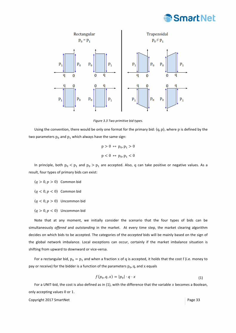
Copyright2017SmartNet Page33
Figure3.3Twoprimitivebidtypes.
Usingtheconvention,therewouldbeonlyoneformatfortheprimarybid: q, p ,wherepisdefinedbythe
twoparametersp3andp4whichalwayshavethesamesign:
p > 0p3, p4 > 0
p < 0p3, p4 < 0
In principle, bothp3 < p4 andp3 > p4 are accepted. Also,q can take positive or negative values. As a
result,fourtypesofprimarybidscanexist:
𝑞 > 0, 𝑝 > 0 Commonbid
𝑞 < 0, 𝑝 < 0 Commonbid
𝑞 < 0, 𝑝 > 0 Uncommonbid
𝑞 > 0, 𝑝 < 0 Uncommonbid
Note that at any moment, we initially consider the scenario that the four types of bids can be
simultaneously offered and outstanding in the market. At every time step, the market clearing algorithm
decidesonwhichbidstobeaccepted.Thecategoriesoftheacceptedbidswillbemainlybasedonthesignof
the global network imbalance. Local exceptions can occur, certainly if the market imbalance situation is
shiftingfromupwardtodownwardorvice-versa.
Forarectangularbid,p3 = p4andwhenafractionxofqisaccepted,itholdsthatthecostf(i.e.moneyto
payorreceive)forthebidderisafunctionoftheparametersp3, q,andxequals
𝑓 𝑝3, 𝑞, 𝑥 = 𝑝3 ⋅ 𝑞 ⋅ 𝑥 (1)
ForaUNIT-bid,thecostisalsodefinedasin(1),withthedifferencethatthevariable𝑥becomesaBoolean,
onlyacceptingvalues0or1.
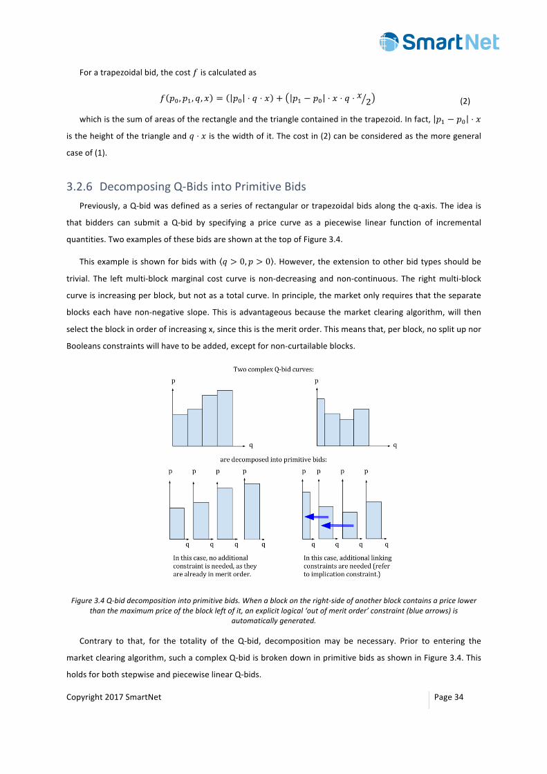
Copyright2017SmartNet Page34
Foratrapezoidalbid,thecost𝑓iscalculatedas
𝑓 𝑝3, 𝑝4, 𝑞, 𝑥 = 𝑝3 ⋅ 𝑞 ⋅ 𝑥 + 𝑝4 − 𝑝3 ⋅ 𝑥 ⋅ 𝑞 ⋅ 𝑥 2 (2)
whichisthesumofareasoftherectangleandthetrianglecontainedinthetrapezoid.Infact, 𝑝4 − 𝑝3 ⋅ 𝑥
istheheightofthetriangleand𝑞 ⋅ 𝑥isthewidthofit.Thecostin(2)canbeconsideredasthemoregeneral
caseof(1).
3.2.6 DecomposingQ-BidsintoPrimitiveBidsPreviously,aQ-bidwasdefinedasaseriesofrectangularortrapezoidalbidsalongtheq-axis.Theideais
that bidders can submit a Q-bid by specifying a price curve as a piecewise linear function of incremental
quantities.TwoexamplesofthesebidsareshownatthetopofFigure3.4.
Thisexampleisshownforbidswith 𝑞 > 0, 𝑝 > 0 .However,theextensiontootherbidtypesshouldbe
trivial. The leftmulti-blockmarginal cost curve is non-decreasing andnon-continuous. The rightmulti-block
curveisincreasingperblock,butnotasatotalcurve.Inprinciple,themarketonlyrequiresthattheseparate
blockseachhavenon-negative slope.This isadvantageousbecause themarket clearingalgorithm,will then
selecttheblockinorderofincreasingx,sincethisisthemeritorder.Thismeansthat,perblock,nosplitupnor
Booleansconstraintswillhavetobeadded,exceptfornon-curtailableblocks.
Figure3.4Q-biddecompositionintoprimitivebids.Whenablockontheright-sideofanotherblockcontainsapricelowerthanthemaximumpriceoftheblockleftofit,anexplicitlogical‘outofmeritorder’constraint(bluearrows)is
automaticallygenerated.
Contrary to that, for the totality of the Q-bid, decomposition may be necessary. Prior to entering the
marketclearingalgorithm,suchacomplexQ-bidisbrokendowninprimitivebidsasshowninFigure3.4.This
holdsforbothstepwiseandpiecewiselinearQ-bids.
Copyright2017SmartNet Page35
IntheleftcaseofFigure3.4,anyblockhasequalorhigherpricesthananyofthepricespresentinitsleft
neighborblock.Thismeansthattheyarealreadyorderedineconomicmeritorder,whichistheorderthatthe
marketwill select theseblocks.Therefore, there isnoneedtoaddconstraints thatablockwillbeaccepted
beforeitsrightneighborblock.Thisessentiallymeansthatthebidderwantsblockstobeacceptedoutofmerit
order.Thiswillhavetobeindicatedbytheadditionofalogicalconstraintthatforcestheleftneighboringblock
ofablocktobeacceptedbeforetheblockitself.
In the right case in Figure 3.4, this leads to a constraint forcing acceptance of the entire second block
beforethethirdcanbeevenpartiallyacceptedandsimilarlyaconstraintforcingthefirstblockbeingentirely
acceptedbeforeanyfractionofthesecondblockcanbeaccepted.Whenx3,x4,xE,andxFaretheacceptance
fractionsoftheblocksdrawnfromlefttorightinFigure3.4,italwaysholdsthatx3 ≥ x4 ≥ xE ≥ xF,sothese
inequalitiescanbeappliedasconstraintsinthemodel.Theseconstraintsareofthelogicalimplicationtypeas
discussedlateron.
Also,weimpose xE ≥ xEx4 = 1 and x4 ≥ x4
x3 = 1 fortherightcaseofFigure3.4,wherexH
is theminimal resolution of the acceptance fraction 𝑥 of the bid 𝑖, with an exemplary value of 0.01. This
minimal resolution brings advantages both in physical activation-limit of assets and in computational
efficiency.Anexampleofthefirstcaseiswhenabatteryassetisactivatedtoinjectwitha0.0001percentof
thebidquantity,whichmaynotbepossibleduetolimitedprecisionofpowerelectronics.Forthesecondcase,
theminimalresolutionhelpsavoidingstorageofvaluestoahighdecimalprecision,allowingroundedvalues
forpowerflows.Thisisindeedincompliancewiththecurrentmarketregulations.
3.2.7 DefinitionofAcceptance
Tobeabletoformulatetemporalconstraintsregardingthenumberordurationofactivationsoverthetime
horizonofaQt-bid,onehas to formulateaconceptof ‘acceptance’of thatbid foreach timestep.Another
reasontodefinethisistobeabletoconstructlogicalrelationsbetweenacceptanceofQ-bidsandbetweenQt-
bids.Note that, for bidswhich are not subject to these constraints and also only composed ofQ blocks in
economicmeritorder,nosingleBooleanvariableisdefined.
ForUNIT-bids,acceptanceofthebidsimplymeansthatanon-zeroquantityisactivated.Ontheotherside,
thelevelofacceptance(fullyorpartially)referstotheactualquantitywhichisactivated.ForQ-bidsandQt-
bids,theformulationofacceptanceisprovidedintheappendixinSection9.1.3.
3.3 CommitmentofMarketDecisions
The rolling optimization of the Integrated Reserve market, as demonstrated in Figure 2.1, raises the
questionofthecommitmentforthemarketdecisions.
To keep amarket as reactive to system state change as possible,we assume that, by default, only the
decisions for the first time-step are firm. The activation information for the other time steps are not a

Copyright2017SmartNet Page36
commitment requestedby themarketoperator to the flexibilityproviders, but informationabout themost
likely future activation decisions if everything in the system stays as planned. By committing the activation
onlyforthefirsttime-step,themarketoperatorkeepsopenenoughdoorstoadapttheactivationdecisionsin
caseofchangeinthesystemstate.
However,someflexibilityassetshavetemporalconstraintsorneedtobeinformedoftheactivationsome
timeinadvance.Namely,biddingcapacityinmarketattimeNisafunctionoftheclearingprocessinmarketat
N-1. For this reason, optional temporal constraints can be added to the market bids and will lead to
anticipative commitment from the market operator. We describe these optional constraints in the next
sections.
3.4 Intra-BidTemporalConstraints
Wedefineamarketwherebidderscanoptionallysupplysometemporalconstraintswitheachoftheirbids.
Therearemultipletypesoftemporalconstraints,butonlyoneconstraintisallowedperbidandperconstraint
type.Notethat inthissection,allconstraintsaredefinedonbids intheformthebiddersupplies(b ∈ BNO),
andnotonthedecomposedprimitivebids(β ∈ ΠNOST).
Thesimplestbalancingmarketwouldnotkeeptrackofanytemporalconstraintsof itsbidders. Insucha
marketsetup,theaggregatorswouldhavetoensurethemselvesthatallpowerquantitiesandallcombinations
ofselectablepowerquantitiesoverthewholebidtimehorizonarefeasibleforthem.
However, doing somay severely limit the offered feasible region of the quantities bidders can present,
sincesometimes their feasible regionsareconditionalon temporal constraints, like, say rampconstraints. If
biddingaggregatorskeeptrackofthesetemporalconstraintsthemselves,theycannotofferquantitiestothe
marketbeyondthefirsttime-step,sincetheydonotknowwhatdecisionthemarketwilltakeinthefirsttime-
step.Therefore,thiswouldmeanonlybidsforthefirsttime-stepwillbeoffered.
This inturndoesnot leverageatall theadvantagesoftwoaspectsoftheproposedoptimization:(i) the
rolling horizon aspect and (ii) the global optimization across all market participants, each with their own
temporalconstraints.Forthesetworeasons,webelievethatofferingthemorecommontemporalconstraints
as a service in the market clearing algorithm is reasonable. Therefore, the approach taken is to include
complexity on the market clearing algorithm, rather than on the bidding algorithm (see discussion about
consultationinSectionFeedbackfromConsultation:Bidding).
In thenextsections,we introduce the6 intra-bid temporalconstraintswhichareallowed in themarket.
DetailedmathematicalformulationofeachconstraintisshownintheappendixinSection9.1.4.
3.4.1 Accept-All-Time-Steps-or-NoneConstraint
Copyright2017SmartNet Page37
This constraint associates to aQt-bid and ensures that either the bid is accepted for all the time steps
consideredinthebidorthatitisnotacceptedatall.Notethatthedefinitionofacceptanceisdifferentfora
non-curtailable,stepcurtailableorpiecewiselinearcurtailablebid.
Intermsofcommitment,thistypeofproductimpliesananticipativecommitmentbythemarketoperator:
ifduringthemarketclearing,aQt-bidwith“Accept-All-Time-Steps-or-None”constraint isaccepted,thenthe
market operator already commits to activate it for all the time steps considered in the Qt-bid and to stay
consistentwiththatfortheconsecutivesoptimizations(atmostuntiltheendofhorizon).
This constraint allows, for example, to submit a specific load-profile that has to be followed when the
correspondingasset isactivated.Furthermore,thisconstraintcanbeusedwhenaccountingfortherebound
effect.MathematicalformulationofthisconstraintisprovidedintheappendixinSection9.1.4.2.
3.4.2 RampingConstraints
A physical energy generation or consumption asset typically has a ramp-up or/and ramp-down energy
production/consumption profile. After aggregation of many assets this may sometimes disappear, but can
sometimes still bepresent.We formulate the ramp-upand ramp-downconstraintsat the resolutionofone
singlemarket clearing decision step, since that is themost accurate level possible. The constraints can be
formulatedas,forexample:
MAX_RAMP_UP_PER_STEP=3
MAX_RAMP_DOWN_PER_STEP=4.
Thismeansthatthemarketclearingalgorithmwilltakecarethat,fromanydecisionsteptothenextone,
injected/extractedactivepower,inabsolutevalue,doesnotincreasebymorethan3MWandthatpowerdoes
notdecreasebymore than4MW.Note that thebid issuers are awareof the fixeddecision time step and
shouldformulatetheirrampingconstraintsaccordingly.Notethatonecanalsospecifyjustoneoftheramping
constraintsseparatelywithouttheother.
Regardingcommitmentaspects,theactivationdecisionsforQt-bidsareonlyfirmforthefirsttime-stepof
therollingoptimizationbuttherampingconstraintlimitswhatitwillbepossibletodointhenextclearing.
Inaninterestingapplication,rampingconstraintscanbesetto
MAX_RAMP_UP_PER_STEP=0,
MAX_RAMP_DOWN_PER_STEP=0,
whichmeansthatthesameamountofpowershouldbeinjected/off-takenforeverytimestepwithinthe
bid-horizon of the (Qt-) bid. In this case, the ramping constraint intrinsically includes an “Accept-All-Time-
Steps-or-None”criterion,asdescribedbefore.
MathematicalformulationoftherampingconstraintisprovidedintheappendixinSection9.1.4.3.

Copyright2017SmartNet Page38
3.4.3 MaximumNumberofActivationsConstraint
Abidissuermaywanttorestrictthenumberofactivationswithinagivennumberofdecisiontimesteps.A
typicalexamplewouldbetoavoidwearandteareffectonmechanicalswitchesoronincandescentlights.This
canbe specifiedbyMAX_N_ACTIVATIONS_PER_STEPS= (X,Y)whereX represents themaximumnumberof
activationsandYtheconsideredtimehorizonforthebid(thatcanbeshorterthanthemarkettimehorizonif
needed).MathematicalformulationofthisconstraintisprovidedintheappendixinSection9.1.4.4.
3.4.4 MinimumandMaximumDurationofActivationConstraint
Abiddermaywanttorestricttheactivationdurationtoagivenminimumnumberofdecisiontimesteps.
Thiscanbespecifiedby
MIN_N_STEPS_PER_ACTIVATION=5.
SupposethataQt-Bidcontains10decisiontimesteps.Thenifthebidisactivated,ithastobeactivatedfor
at least5subsequenttimestepswithinthese10timesteps.Obviously,MIN_N_STEPS_PER_ACTIVATIONcannot
be larger than the number of time steps contained in the Qt-bid. The default value for
MIN_N_STEPS_PER_ACTIVATIONis0.
Similarly, abiddermaywant to restrict theactivationduration toa givenmaximumnumberofdecision
timesteps.AtypicalexampleofthisconstraintisthecaseofanHVACsystemwherethereisamaximumtime
period that theHVACcanbestoppedbefore thediscomfort level isunacceptable for theusers.Thiscanbe
specifiedby
MAX_N_STEPS_PER_ACTIVATION=10.
Thedefault value forMAX_N_STEPS_PER_ACTIVATION is equal to thenumberofdecision time steps in the
bid. The time a bid is active is defined between the beginning of activation and the end of that same
activation.Notethatasinglebidcanhaveseveralactivationsoveritsbidtimehorizon.
MathematicalformulationoftheseconstraintsisprovidedintheappendixinSection9.1.4.5.
3.4.5 MinimalDelayBetweenTwoActivations
Similar to theprevious constraints, abiddermayneed to specify theminimumtimedelaybetween two
consecutiveactivations,whichcanbeusefulforexamplewhentheassethasacool-downorstart-upduration.
MathematicalformulationofthisconstraintisprovidedintheappendixinSection9.1.4.6.
3.4.6 IntegralConstraint
Copyright2017SmartNet Page39
For some types of flexible assets, we want to express temporal constraints in terms of the integral of
injection/off-takeofactivepowerovertheconsideredtimehorizon.
Thisconstraintcanforcethepower-integraltobeatafixedvalue(e.g.zero)ortobebetweenalowerand
anupperbound,specifiedby:
INTEGRAL_Target=E
or
INTEGRAL_Bound=(L,U)
where𝐸representstheenergytargetintermsofintegralofactivepowerinjection/offtakeoverthetime
horizonandwhere𝐿and𝑈representsthepotentiallowerandupperboundonthisintegral,respectively.
Intermsofcommitment,theactivationdecisionisonlyfirmforthefirsttime-stepbutthisfirstactivation
decisionhasimplicationonwhatcanbedoneforthenexttimestepsandnextclearings,aswekeeptrackof
theintegralconstraint.
For a consumer bid, the integral constraint is intended to formulate that the total energy consumption
shouldremainunchangedoverthebidhorizon.Forsheddableloads(suchasthermostaticloads),itismeantto
assurethattheset-point(andhencethecomfortorschedule)ismaintained.Forshiftableloads(alsoknownas
atomic loads, suchasa factoryproduction lineoranaggregationofwetappliances), it guarantees that the
profileofdemandisfollowingthescheduledpattern.
Formulatingsuchaconstraintonabidreflectsthelimitsonbothupwardanddownwardflexibilityofthe
bidder’sassetswithinthebidhorizon.Additionally,thisconstraintcanbeappliedtogeneratorassets,incase
theownerwouldliketohaveaguaranteedamountofproductionperhorizon(andhenceachieveaminimum
amountofrevenue).
MathematicalformulationofthisconstraintisprovidedintheappendixinSection9.1.4.7.
3.5 Inter-BidLogicalConstraints
Intheprevioussection,wehavedescribeddifferentoptionaltemporalconstraintsthatcanbeassociated
withoneQt-bid.Wecanalsoallowlogicalconstraintsthatlinktheacceptanceornon-acceptanceofmultiple
bidssubmittedbythesamebidder.Thismeansthatthelogicalconstraintswouldbeinter-bidconstraints.
These constraints are applied to two or more separate bids and define a logical relation between the
Booleanswhichruletheiracceptance.NotethatacceptanceforaQt-bidisdefinedasacceptanceforanytime
step.Abiddercanchangethisdefinitiontoacceptance-at-all-time-stepsbyspecifying“acceptalltimestepsor
none”perbid,asdiscussedbefore.
Foreverybidthatoccursinalogicalconstraint,aBooleanvariablewillthenautomaticallybemodelledin
themarketclearingmodel.Thisvariablerepresentsthatabid isaccepted,partiallyortotally.Sinceinter-bid
Copyright2017SmartNet Page40
constraintsneedtorefertomultipledifferentbids,weneedasystemtouniquelyidentifythem.Weusethe
(BID_ISSUER_ID,BID_ID)-pairsalreadydiscussedforthatpurpose.
3.5.1 ImplicationConstraint
Itisacommonpracticetoallowthemarkettoselectabidonlyifanotherbidhasbeenacceptedaswell.
Thiscouldforexamplerepresenttwo interrelatedflexibleprocesseswherethesecondonecanbeactivated
onlyifthefirstoneisalsoactivated.
This constraint, called the implication, is modelled by introduction of Boolean variables bool1, bool2
associatedwiththebidsb1andb2(1ifthebidisaccepted,0otherwise)andaddingtheconstraintbool1
bool2. This then means that if b1 is accepted, b2 will also be accepted. Implication constraints are only
possiblebetweenbidssubmittedforthesamenetworknodeandbelongingtothesamebidder.
Sucharelationcouldbeformulatedbyabidissueras,forexample:
(BID_ISSUER_ID=100.101.102.1,IMPL_ACCEPT,BID_ID=22,BID_ID=21)
Thismaybe the case for a primitive bid (within aQ-bid string) that has a lowermarginal cost than the
primitivebidinalowerquantity,ashasbeendiscussedintherighthalfofFigure3.4.Inthiscase,thebidders
do not generate the acceptance implication constraint. Instead, at the bid decomposition stage, these
constraintsareautomaticallygenerated.
Anothersituationwhereaccesstoactivationofasecondbidisconditionalontheactivationofafirstbidis
givenhere.Inaproductionprocess,asecondprocessmaybesimultaneous,butoptionaltoafirstone.Inthat
case, theactivationof thebid representing thesecondprocess implies that thebid representedby the first
processisactivated.
If the implication constraint holds in both directions between bids, one should consider the question if
then, these bids cannot simply be aggregated into one bid instead. Looped implication constraints (i.e. the
acceptanceofbid1subjecttobid2,acceptanceofbid2subjecttobid3,andacceptanceofbid3subjectto
bid1)areallowed,assuchloopsexistintoday’sEuropeanday-aheadelectricitymarket.
MathematicalformulationofthisconstraintisprovidedintheappendixinSection9.1.4.8.
3.5.2 ExclusiveChoiceConstraint
Theexclusivechoiceconstraint(alsoknownasEXORconstraint)isusedtoindicateanexclusiveacceptance
betweenasetofbids.Forexample, ifanaggregatorhasanassetthatcouldmovetoanumberofexclusive

Copyright2017SmartNet Page41
statesduringthenexttimestep(suchasanatomicload),thecorrespondingbidsshouldbeaccompaniedbyan
exclusivechoiceconstraint9.
Sucharelationcouldbeformulatedbyabidissueras,forexample:
(BID_ISSUER_ID=100.101.102.1,EXOR_ACCEPT,BID_ID=22,BID_ID=7,BID_ID=8,BID_ID=30)
MathematicalformulationofthisconstraintisprovidedintheappendixinSection9.1.4.9.
3.5.3 DeferabilityConstraint
Ifthebidderhastheflexibilityofdeferringitsbid,itcandosobyspecifyingthemaximumdeferability(i.e.
themaximumdelayintheacceptance)intermsofthenumberoftimesteps.Themarketcanalsoleveragethis
additionalflexibilitytodeterminethetime-shiftthatbestresolvesitsimbalanceproblem.
Anexampleisaprocesswithagivenfixedloadprofile(definedusingaQt-bidwithonegivenquantityper
time and an “Accept-All-Time-Steps-or-None” constraint) which has a flexible starting time, allowing the
markettoactivateitforthecurrenttimesteporshiftitifneeded.
MathematicalformulationofthisconstraintisprovidedintheappendixinSection9.1.4.10.
3.6 IncludingReactivePowerinBids
Untilnow,weonlydiscussedtheformulationofbidsandconstraintswhicharerelatedtotheflexibilityof
activepower.However, if it is intended that themarketprevents violationof voltage constraints, theasset
havetoprovideinformationabouttheirrangeofflexibilityoninjection/off-takeofreactivepower.Inaddition,
anoptimalmanagementofthereactivepowerwouldallowahigherexploitationoftheactivepowerpotential
ofdistributionresources.
The relationship between the active and reactive power for a certain asset (or a group of aggregated
assets)isdefinedusingthepowerfactor(PF).Thereareseveraloptionstodefinethelimitationofthepower
factor:
1. Fixedpowerfactor
2. TriangularP-Qlimits
3. RectangularP-Qlimits
4. CircularP-Qlimits
Figure3.5providesagraphicalrepresentationoftheseoptions.
9TheExclusiveChoiceconstraintisdefinedpertimestepandisnotautomaticallycarriedontothenexttimestep.

Copyright2017SmartNet Page42
Figure3.5GraphicalrepresentationofvariousP-Qlimitdefinition:a)fixedpowerfactor,b)triangularlimit,c)rectangularlimit,d)circularlimit.
Somepointsofattentionabouttheprovisionofinformationonreactivepowerandthemarketclearingatthe
presenceofreactivepowerbidsarelistedhere.
• Thereactivepowershouldhaveazeroprice.Giventhis, themarketwillhavethefreedomofactivating
reactivepowerresourcestoreachfeasibilitywithoutsacrificingthesocialwelfare.Itisalsocriticalthatthe
reactivepowerisactivatedonlywhenitisnecessarytoavoidviolatingaconstraint:
o Theprovisionofreactivepowerflexibilityatzerocostisconsideredrealisticanditisalready
amandatoryserviceinsomeoftheEuropeancountries.
o The“activationonlyinnecessity”ismeanttoavoidreactive-powerexchangewhenitisnot
necessary.Thiscanbeimplementedbyassigningasmallpricetoreactive-powerexchange.
Thishastobefurtherinvestigated.
• Themarketclearingalgorithmhasthepossibilityofincludingreactivepowerinthebids:
o Rectangularandtriangularcapabilitiescanbeeasilyimplemented.
o Implementing fixed power-factor capabilities are more difficult, as they may still lead to
infeasibilities.However,thisproblemcanbetackledbymodelingthegrid-ownedassetssuch

Copyright2017SmartNet Page43
as capacitor banks, which can be used to compensate for the lack of reactive-power
flexibility.

Copyright2017SmartNet Page44
4 GridModel forMarketClearing:Trade-Offs inTractability,Accuracy,andNumericalAspects
4.1 Introduction
In the SmartNet project, it is the aim to develop amarket clearingmethodology that takes the power
system’sphysicallimitsintoaccount.
In current best practices, the part of the power system participating in the market is considered as a
copperplate,whereastheinteractionwithotherzonesisconsideredthroughanetworkflowapproximation.
To avoid problems due to the limited accuracy of such models, a post-clearing AC power flow check is
performed and re-dispatch canbe performed in case of expectedoperational difficulties. Such actionsmay
lead to inefficiency. Including a more accurate network model in the market clearing will help to avoid
countertradingandtheassociatedcosts,especiallywhenconsideringdistributiongrids.
However, taking thephysicsofpower flow intoaccount,while guaranteeing solution times in real time,
demands pragmatic approaches. Convexification and linear approximation of the equations describing the
physical system are two such approaches to improve computational tractability, which will be detailed
throughoutthischapter.
Generically, including power system’s physics into a market clearing methodology implies solving an
OptimalPowerFlow(OPF)problem.Therefore,thischapterstartswithanoverviewonchallengesinoptimal
powerflowcalculations,andrecentadvancesinOPFrelaxationsandapproximations.
4.2 ChallengesinOptimalPowerFlow
4.2.1 OptimalPowerFlow
Optimal power flow (OPF) has been a topic of interest for 50 years,with Carpentierwriting his seminal
paper in 1962 [6]. He, amongst other things, concluded that the convexity of the problem was to be
researchedfurther.DommelandTinney[7]in1968developedpracticalcalculationmethods,andsolvedcase
studiesof500nodes.AlsacandStottwidened the scopeof thesemethods in1973 through the conceptof
security-constrainedOPF(SCOPF)[8],[9].AreviewofrecentSCOPFliteratureispublishedbyCapitanescu[10].
Ingeneral,OPFencompassesanypowersystemoptimizationproblemwithphysicalpowerflowaspartof
themodel.Thisdoesnotexcludemuch,thereforeOPFingeneralcanbe:multiperiod,security-constrained,DC
orAC,orbasedonapproximations.

Copyright2017SmartNet Page45
Power flow is generally considered as a complex-valued problem. Two formulations of the power flow
equationshavebeenusedwidely:aquadraticone,basedontherectangular-complexnotation,andapolar-
complexone,usingsineandcosinefunctions.Finally,BaranandWudevelopedaninterestingformulationof
thepowerflowequationsin1989[11],whichsimplifiedpowerflowmodelinginradialgrids.Thisformulation
ofthepowerflowequationsiscalledDistFlow.
4.2.2 ConvexRelaxationApproaches
Sincequite awhile it hasbeenunderstood that the truedistinctionbetweeneasy-to-solve andhard-to-
solveproblemsdoesnotalignwithlinearprogramming(LP)versusnonlinearprogramming(NLP)problemsbut
withconvexversusnonconvexoptimization. In theoryand inpractice, largeconvexproblemscanbesolved
reliably (convergence guarantees), quickly (polynomial-time) and to global optimality. With nonconvex
(smooth) optimization, one largely has to choose between solving problems quickly but locally optimal or
globallyoptimalbutslowly.Withthedevelopmentofpracticalsemidefiniteprogramming(SDP)methods[12],
effortshavebeenmadeto leveragetheirexpressivepowertofindstrongSDPapproximationstononconvex
problems.Ahierarchyofcontinuousoptimizationcomplexityclassescanbedevelopedasfollows:
LP ⊂ QP ⊂ CQCP ⊂ SOCP ⊂ SDPabNcde
⊂ NCQCP ⊂ NLPNbNabNcde
Anynonconvexquadratically constrainedoptimizationproblem (NCQCP) canbe reformulated as an SDP
problem with the addition of a nonconvex rank constraint. After removal of the rank constraint (Shor’s
relaxation [13]), a SDP problem remains, which can be solved with SDP solvers. This step of removing
nonconvexconstraintsisreferredtoasthe‘convexrelaxation’.Thepowerflowequationsareeasilywrittenas
asetofnonconvexquadraticequations;therefore,thisstrategycanalsobefollowed.Onetherebyobtainsthe
SDPrelaxationofOPF.
Relaxations,byaprocessofonlyremovingequationsfromthefeasiblesetofanoriginalproblem,provide
strongqualityguaranteesonthesolutionofbothproblems:
• iftheoriginalproblemisfeasible,therelaxedproblemisfeasible;
• iftherelaxedproblemisinfeasible,theoriginalproblemisinfeasible;
• theoptimumof the relaxedproblemwill be a lowerbound (minimization) for theoptimumof the
originalproblem.
Approximations(whichcannotbeshowntoberelaxations),donotprovidesuchguarantees.Nevertheless,
the idea is that they are sufficiently accurate, but only under certain conditions. More generally, convex
relaxationscanbeobtainedforpolynomiallyconstrainedpolynomialprograms,forwhichmomentrelaxation
strategies have been developed [14]. Moment relaxations are tighter than the previously-discussed SDP
relaxations,asthisSDPrelaxationisjustthefirst-ordermomentrelaxation.
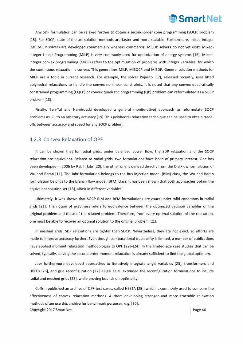
Copyright2017SmartNet Page46
AnySDPformulationcanberelaxedfurthertoobtainasecond-orderconeprogramming(SOCP)problem
[15]. For SOCP, state-of-the-art solutionmethods are faster andmore scalable. Furthermore,mixed-integer
(MI) SOCP solvers aredeveloped commerciallywhereas commercialMISDP solvers donot yet exist.Mixed-
integer Linear Programming (MILP) is very commonly used for optimization of energy systems [16].Mixed-
integerconvexprogramming(MICP)referstotheoptimizationofproblemswith integervariables, forwhich
thecontinuousrelaxationisconvex.ThisgeneralizesMILP,MISOCPandMISDP.Generalsolutionmethodsfor
MICP are a topic in current research. For example, the solver Pajarito [17], released recently, uses lifted
polyhedral relaxations to handle the convexnonlinear constraints. It is noted that any convexquadratically
constrainedprogramming(CQCP)orconvexquadraticprogramming(QP)problemcanreformulatedasaSOCP
problem[18].
Finally, Ben-Tal and Nemirovski developed a general (noniterative) approach to reformulate SOCP
problemsasLP,toanarbitraryaccuracy[19].Thispolyhedralrelaxationtechniquecanbeusedtoobtaintrade-
offsbetweenaccuracyandspeedforanySOCPproblem.
4.2.3 ConvexRelaxationofOPF
It can be shown that for radial grids, under balanced power flow, the SDP relaxation and the SOCP
relaxation are equivalent. Related to radial grids, two formulations have been of primary interest.One has
beendevelopedin2006byRabihJabr[20],theotheroneisderiveddirectlyfromtheDistFlowformulationof
WuandBaran [11].The Jabr formulationbelongs to thebus injectionmodel (BIM)class, theWuandBaran
formulationbelongstothebranchflowmodel(BFM)class.Ithasbeenshownthatbothapproachesobtainthe
equivalentsolutionset[18],albeitindifferentvariables.
Ultimately, itwas shownthatSOCPBIMandBFMformulationsareexactundermildconditions in radial
grids [21]. The notion of exactness refers to equivalence between the optimized decision variables of the
originalproblemandthoseoftherelaxedproblem.Therefore,fromeveryoptimalsolutionoftherelaxation,
onemustbeabletorecoveranoptimalsolutiontotheoriginalproblem[21].
Inmeshed grids, SDP relaxations are tighter than SOCP.Nevertheless, they arenot exact, so efforts are
madetoimproveaccuracyfurther.Eventhoughcomputationaltractabilityislimited,anumberofpublications
haveappliedmomentrelaxationmethodologiestoOPF[22]–[24].Inthelimited-sizecasestudiesthatcanbe
solved,typically,solvingthesecondordermomentrelaxationisalreadysufficienttofindtheglobaloptimum.
Jabr furthermore developed approaches to iteratively integrate angle variables [25], transformers and
UPFCs [26], and grid reconfiguration [27].Hijazi et al. extended the reconfiguration formulations to include
radialandmeshedgrids[28],whileprovingboundsonoptimality.
CoffrinpublishedanarchiveofOPFtestcases,calledNESTA[29],whichiscommonlyusedtocomparethe
effectiveness of convex relaxation methods. Authors developing stronger and more tractable relaxation
methodsoftenusethisarchiveforbenchmarkpurposes,e.g.[30].
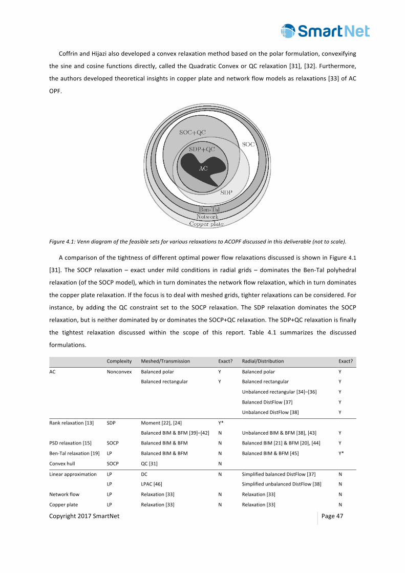
Copyright2017SmartNet Page47
CoffrinandHijazialsodevelopedaconvexrelaxationmethodbasedonthepolarformulation,convexifying
thesineandcosine functionsdirectly,calledtheQuadraticConvexorQCrelaxation[31], [32].Furthermore,
theauthorsdevelopedtheoreticalinsightsincopperplateandnetworkflowmodelsasrelaxations[33]ofAC
OPF.
Figure4.1:VenndiagramofthefeasiblesetsforvariousrelaxationstoACOPFdiscussedinthisdeliverable(nottoscale).
AcomparisonofthetightnessofdifferentoptimalpowerflowrelaxationsdiscussedisshowninFigure4.1
[31]. The SOCP relaxation – exact undermild conditions in radial grids – dominates the Ben-Tal polyhedral
relaxation(oftheSOCPmodel),whichinturndominatesthenetworkflowrelaxation,whichinturndominates
thecopperplaterelaxation.Ifthefocusistodealwithmeshedgrids,tighterrelaxationscanbeconsidered.For
instance, by adding the QC constraint set to the SOCP relaxation. The SDP relaxation dominates the SOCP
relaxation,butisneitherdominatedbyordominatestheSOCP+QCrelaxation.TheSDP+QCrelaxationisfinally
the tightest relaxation discussed within the scope of this report. Table 4.1 summarizes the discussed
formulations.
Complexity Meshed/Transmission Exact? Radial/Distribution Exact?
AC Nonconvex Balancedpolar Y Balancedpolar Y
Balancedrectangular Y Balancedrectangular Y
Unbalancedrectangular[34]–[36] Y
BalancedDistFlow[37] Y
UnbalancedDistFlow[38] Y
Rankrelaxation[13] SDP Moment[22],[24] Y*
BalancedBIM&BFM[39]–[42] N UnbalancedBIM&BFM[38],[43] Y
PSDrelaxation[15] SOCP BalancedBIM&BFM N BalancedBIM[21]&BFM[20],[44] Y
Ben-Talrelaxation[19] LP BalancedBIM&BFM N BalancedBIM&BFM[45] Y*
Convexhull SOCP QC[31] N
Linearapproximation LP DC N SimplifiedbalancedDistFlow[37] N
LP LPAC[46] SimplifiedunbalancedDistFlow[38] N
Networkflow LP Relaxation[33] N Relaxation[33] N
Copperplate LP Relaxation[33] N Relaxation[33] N
Copyright2017SmartNet Page48
Table4.1Categorizationofformulations.
4.2.4 FurtherBackground
Theupcomingparagraphs discuss a number ofworkswhich summarize and generalize a number of the
previouslydiscussedarticles,aswellasdevelopcasestudiesbasedontheproposedmethods.
An in-depthreviewofOPFmethodologieswasperformedbyFERCandaseriesof reportswaspublished
[47],includingarticlessuchas[48].Morerecently,Capitanescupublishedareviewofdevelopmentsrelatedto
ACOPFcalculation,includingadiscussionontheeffectivenessofconvexificationstrategies[49].
Early2015,JoshuaTaylorpublishedabookonconvexoptimizationmethodsforpowersystems[18].This
wellwrittenworksummarizesthestate-of-the-artofconvexOPFmethodsinasingleformalism,whichmakes
thisbookaneasyentrypointtothefield.
Steven Low developed a convex OPF literature study [50] and published a tutorial-style article to get
startedwith the convex OPF formulations [51]. Lingwen Gan, a former doctoral student of Low, wrote his
doctoraldissertationontheapplicationoftheconvexificationmethodsinradialgrids[52].
GanandLowregularlydiscussedthe‘exactness’oftheconvexformulations[53]–[55].JavadLavaeifocused
hiseffortsontheSDPformulationandpublishedanimplementationofthisproblemforMatlab[56],inwhich
healsodevelopsapenalizationapproach.Healsopublishedsomeinsightsintotheeffectivenessoftheconvex
relaxationsofOPFbasedoninsightinthephysicsunderlyingtheproblem[57].
Anya Castillo, in her doctoral dissertation, developed a number of ACOPF formulations (nonconvex,
convex),methods (global, local) and case studies (storage) [58]. In his dissertation, titled ‘Optimization and
control of power flow in distribution networks’, Masoud Farivar develops convex models for OPF in
distributiongrids[59].Heincludesvolt-varcontrolanddevelopsanumberofcasestudies.
4.3 ConvexRelaxationFormulations
Twomain formulations of convex relaxations of the power flow equations have been of interest in the
scientific literature: the bus injection model (BIM) and the branch flow model (BFM) formulation. These
relaxationshavebeenshowntobeequivalent[50].
TheQuadraticConvexorQCformulation,beingbasedonadifferentrelaxationprocess(combiningconvex
hulls) [30], is not equivalent to those formulations. Therefore, adding any non-dominatedQC constraint to
either the BFM or BIM formulation can result in a tighter overall formulation, as the formulations can be
combined.
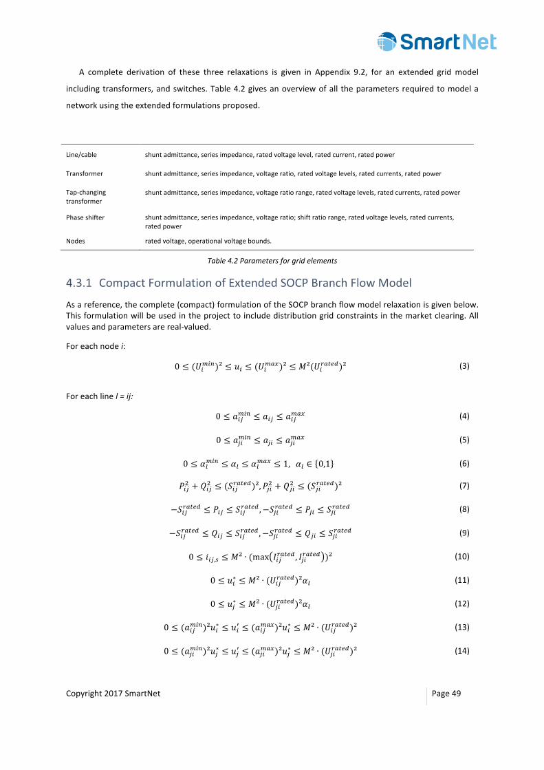
Copyright2017SmartNet Page49
A complete derivation of these three relaxations is given in Appendix 9.2, for an extended grid model
includingtransformers,andswitches.Table4.2givesanoverviewofall theparametersrequiredtomodela
networkusingtheextendedformulationsproposed.
Line/cable shuntadmittance,seriesimpedance,ratedvoltagelevel,ratedcurrent,ratedpower
Transformer shuntadmittance,seriesimpedance,voltageratio,ratedvoltagelevels,ratedcurrents,ratedpower
Tap-changingtransformer
shuntadmittance,seriesimpedance,voltageratiorange,ratedvoltagelevels,ratedcurrents,ratedpower
Phaseshifter shuntadmittance,seriesimpedance,voltageratio;shiftratiorange,ratedvoltagelevels,ratedcurrents,ratedpower
Nodes ratedvoltage,operationalvoltagebounds.
Table4.2Parametersforgridelements
4.3.1 CompactFormulationofExtendedSOCPBranchFlowModel
Asareference,thecomplete(compact)formulationoftheSOCPbranchflowmodelrelaxationisgivenbelow.Thisformulationwillbeusedintheprojecttoincludedistributiongridconstraintsinthemarketclearing.Allvaluesandparametersarereal-valued.
Foreachnodei:
0 ≤ (𝑈)()*)² ≤ 𝑢) ≤ (𝑈)(+,)² ≤ 𝑀²(𝑈)k+lmn)² (3)
Foreachlinel=ij:
0 ≤ 𝑎)p()* ≤ 𝑎)p ≤ 𝑎)p(+, (4)
0 ≤ 𝑎p)()* ≤ 𝑎p) ≤ 𝑎p)(+, (5)
0 ≤ 𝛼r()* ≤ 𝛼r ≤ 𝛼r(+, ≤ 1, 𝛼r ∈ 0,1 (6)
𝑃)pE + 𝑄)pE ≤ (𝑆)pk+lmn)², 𝑃p)E + 𝑄p)E ≤ (𝑆p)k+lmn)² (7)
−𝑆)pk+lmn ≤ 𝑃)p ≤ 𝑆)pk+lmn, −𝑆p)k+lmn ≤ 𝑃p) ≤ 𝑆p)k+lmn (8)
−𝑆)pk+lmn ≤ 𝑄)p ≤ 𝑆)pk+lmn, −𝑆p)k+lmn ≤ 𝑄p) ≤ 𝑆p)k+lmn (9)
0 ≤ 𝑖)p,t ≤ 𝑀² ∙ (max 𝐼)pk+lmn, 𝐼p)k+lmn )² (10)
0 ≤ 𝑢)∗ ≤ 𝑀² ∙ (𝑈)pk+lmn)²𝛼r (11)
0 ≤ 𝑢p∗ ≤ 𝑀² ∙ (𝑈p)k+lmn)²𝛼r (12)
0 ≤ (𝑎)p()*)²𝑢)∗ ≤ 𝑢)z ≤ (𝑎)p(+,)²𝑢)∗ ≤ 𝑀² ∙ (𝑈)pk+lmn)² (13)
0 ≤ (𝑎p)()*)²𝑢p∗ ≤ 𝑢pz ≤ (𝑎p)(+,)²𝑢p∗ ≤ 𝑀² ∙ (𝑈p)k+lmn)² (14)
Copyright2017SmartNet Page50
−𝑀E 𝑈)pk+lmnE1 − 𝛼r ≤ 𝑢) − 𝑢)∗ ≤ 𝑀E 𝑈)pk+lmn
E1 − 𝛼r (15)
−𝑀E 𝑈p)k+lmnE1 − 𝛼r ≤ 𝑢p − 𝑢p∗ ≤ 𝑀E 𝑈p)k+lmn
E1 − 𝛼r (16)
𝑃)pE + 𝑄)pE ≤ (𝐼)pk+lmn)²𝑢)𝛼r (17)
𝑃p)E + 𝑄p)E ≤ (𝐼p)k+lmn)²𝑢p𝛼r (18)
𝑃)p + 𝑃p) = 𝑔)p,t|𝑢)z + 𝑟r,t𝑖)p,t + 𝑔p),t|𝑢pz (19)
𝑄)p + 𝑄p) = −𝑏)p,t|𝑢)z + 𝑥r,t𝑖)p,t − 𝑏p),t|𝑢pz (20)
𝑃)p − 𝑔)p,t|𝑢)zE+ 𝑄)p + 𝑏)p,t|𝑢)z
E≤ 𝑖)p,t𝑢)z (21)
𝑢pz − 𝑢)z = −2 𝑟r,t 𝑃)p − 𝑔)p,t|𝑢)z + 𝑥r,t 𝑄)p + 𝑏)p,t|𝑢)z + (𝑟r,tE + 𝑥r,tE )𝑖)p,t (22)
Note that thenodebalanceequations still need tobeadded inorder toobtain the completeOPFproblemformulation.
4.4 ImpactofFormulationandRelaxation
TheSOCPconvexrelaxationsofthepowerflowequations(givenintheappendixinSection9.3.3.2),havea
number on consequences on the possible result of the initial optimal power flow problem. Also, the
formulationsgivenmayperformdifferentlyfromanumericalpointofview.Adiscussionofanumberofthese
consequencesisfoundbelow.
4.4.1 NumericalStability
LingwenGannotesthattheBFM(DistFlow)formulationhasnumericaladvantagesabovetheBIM[38]for
unbalanced power flow formulations (SDP). This suggests that this may also be the case for balanced
formulations,eventhoughtheeffectmayonlybeobservedforlarge-scaleor‘difficult’problemcases.
In theBFM formulation, thecomplexcurrentandvoltagevariablesare replacedby squaredcurrentand
voltage magnitude variables. Note that the accuracy of these squared variables is impacted by the
reformulation process. For instance, for a numerical accuracy of 10-6 of the reformulated problem in the
squaredcurrentandvoltagemagnitude,inpost-processing,anaccuracyofonly 10�� = 10�Fisobtainedfor
thecurrentandvoltagemagnitude.
4.4.2 Scaling
Copyright2017SmartNet Page51
Thescalingofthesquaredvariablesisimportant.Therefore,isbesttomakesurethatthesquaredvariables
are scaled so that they have a numerical value around 1. This is commonly performed as part of the
transformationofSIunitstotheper-unitbase,butmoreaccuratebasescanbeenvisionedifnecessary10.
4.4.3 Variables
Ascurrent finds thepathof least resistance,KCLcanalsobe thoughtofasminimizing thegrid losses in
electriccircuits[60]–[62].InmeshedACgrids,however,thisisnotgenerallyassimpleduetothevoltagephase
angleconstraints(addinguptozero)thatapplyinloops.IntheDistFlowderivation,thevoltageanglevariables
are substituted out in the SOCP formulations. The SOCP formulations introduce phase shifters in any grid
element,furthermoremakingthevoltageangleconstrainttriviallyfeasible.Voltageanglevariablescanonlybe
partiallyincorporatedagainthroughtheQCfeasibleset.
4.4.4 ConvexificationSlack
The SOCP relaxation by definition introduces nonphysical solutions: those forwhich (𝑃)p,t)E + (𝑄)p,t)E is
strictlylessthan(𝑖)p,t ∙ 𝑢)z)inthefeasibleset.Non-negligibleconvexificationslackinvalidatestheoverallresult
fromthephysicalperspective.Slackmaybeobservedwhenitisbeneficialtohaveincreasedlossessomewhere
inthegrid.Slackrepresents‘free’nonphysicallosses,ontopofthenormalphysicalpowertransferlosses.Such
controllable‘losses’,likeadispatchableload,canbeusedtoeasethegridoperationindifficultcircumstances.
For example, in case of overvoltage, such losses actually help you to bring down the voltage, allowing the
solvertofind(mathematical)solutionsthat‘comply’witha‘difficult’overvoltagelimit.Similareffectscanbe
observedwithcurrentandapparentpowerbounds. It isnotedthat thisslackcannotbeobservedwhenthe
operationalenvelopesareabsent.
If the convexified OPF is infeasible, this guarantees that the original problem is infeasible. However,
infeasibility of the original problem does not guarantee that the relaxed problem returns a certificate of
infeasibility. Incertaincases,anumericalbutnonphysical solution is returned,due to the interactionof the
powerflowandtheoperationalenvelope[21]. Inthiscase, infeasibilityoftheunderlyingproblemhastobe
confirmed.
4.4.5 Penalties
TheBIMSDPandSOCPrelaxationareequivalentforradialgrids.Furthermore,aSOCPconvexrelaxationin
theBFMexpressionisobtainedbydroppingarankconstraintinthenon-convexquadraticconstraint.10 For instance, due to static transformer taps (e.g. 1.1pu), theper unit base canbeoff-set (e.g. nominal 20 kV)withrespecttothebestnumericalbase(e.g.closerto22kV).
Copyright2017SmartNet Page52
Toobtain rank-1 solutions in SDPproblems, rankminimizationheuristics [63]–[65]weredeveloped. The
rankconstraintistherebyreplacedwithapenalty.Insomecases,ahiddenrank-1solutionisrecoveredinthe
original(global)optimum,inothers,someactualincreaseinthecostsisobservedduetothepenalization.The
applicationofsuchheuristicisillustratedby[41],[66],[67],forthebalancedBIMSDPformulation.
Therefore, in case the relaxation is not exact, one can choose to penalize as such, to obtain a solution
withoutconvexificationslack.Itisnotknownwhichpenaltymakesiteasiesttorecoveraglobalornear-global
optimal solution.Twoaspects canbe considered: the formulationand scalingof thepenalty, aswell as the
applicationofthepenaltytoaselectionortoallgridelements.Intheimplementation,onehastochooseto
penalizejustthelinesforwhichtheconvexrelaxationisnotexact,versusbydefaultpenalizingalllinesorno
linesatall.
4.4.6 Objective
Thegoalistofindasolutiontocostminimizationproblem,wheretheobjectiveisaconvexcostfunctionin
thedecisionvariables.Forexample,theobjectiveistominimizethecostofdispatchsubjecttothepowerflow
physicsofadistributiongrid. IntheconvexifiedSOCPOPF, theoriginalproblemhastobecombinedwitha
penalization objective. This penalty is there tomake sure that a solution is found on the boundary of the
solution space (and is thus a feasible solution). The convexification penalties defined are convex and the
feasiblesetistheintersectionofconvexcones(polyhedra,spectahedra).Forradialgrids,itisknownthatthe
convexrelaxationisexactandaphysicalsolutioncanberecoveredifitislocatedonthesurfaceoftheSOCs.
Therefore,theeffectiveobjective isaconvexcombinationoftheoriginalobjectiveYcostandthepenalty
YPFconvex.Thereisachallengeinfine-tuningtheweightofthepenaltyintheproblemobjective.Forapenalty,
whichistoolow,theresultisnotphysical.Forapenalty,whichistoohigh,resultsarephysical,butthecosts
aresuboptimal.Forthelowestpossiblepenaltyforwhichtheslackontheconvexificationis(closeto)zero,the
optimumisobtained.Notethat thecostscanneverthelessbeconstant forawiderangeofpenalties,which
means that fine-tuning of the penaltyweightmay not be required inmost cases.Nevertheless, in cases of
overcurrentandovervoltage,itisexpectedthattheobjectivemaybeverysensitivetothepenaltyweight.
Asearchalgorithmcanbeusedto findthispenaltyweight.Oneapproachto findsuchapenaltyweight,
without use of derivatives, is the bisection method, as proposed by [67]. Note that due to the nature of
interiorpoint algorithms, it is hard toobtain solutions very close to (oron) theedgeof the solution space.
Conversely, simplex-based methods naturally find solutions on the edge of the solution space (but only
supportpolyhedralfeasiblesets,thereforetheBen-Talreformulationtechniquemustbeappliedfirst).
4.5 ApproximatedOPFFormulations
Approximations, conversely to relaxations, do not offer strong general quality guarantees, nevertheless,
theyarewidelyusedbecauseoftheirsimplicity.Twocommonapproximationsexist,thelinearized‘DC’OPF,
Copyright2017SmartNet Page53
commonlyusedintransmissionsystemmodellingandthesimplifiedDistFlow,commonlyusedindistribution
systemmodelling. The feasible setsobtained inboth cases are linear, allowing thedirect applicationof the
morewidelyunderstoodLPmodelingtoolsandsolvers.
InSmartNet, the linearized ‘DC’approximationwillbeusedtomodel thephysicalgridconstraintsof the
transmissiongrid. In linearized ‘DC’OPF, voltagemagnitudes are assumed tobe close to1pu.Conduction
lossesareneglected.Furthermore,resistanceisassumedtobesmallcomparedtoreactance.Finally,voltage
angledifferencesovergridelementsareassumedtobesmall.
Note thatpower flow indistributiongridsviolates theseassumptions:voltagemarginsare larger than in
transmissiongrids,andresistanceandreactancearesimilarinmagnitude.
Coffrin and Van Hentenryck discuss the validity of the linearized OPF in [46]. They note that the ‘DC’
approximationworks reasonablywell activepower flow through largely inductive lines.However, the same
quality of approximation does not hold for the reactive power balance, where stronger nonlinearities are
observed.Therefore,itishardtoincludevoltagemagnitudeconstraintsin‘DC’OPF.
In the simplified DistFlow formulation, it is assumed that the series conduction losses are negligible.
Simplified DistFlow can be considered as the outcome of a low-accuracy Ben-Tal relaxation applied to the
convex DistFlow formulation. Losses are neglected, which results in an error on the power flow of a few
percent.As thepowerconsumedbygrid lossesalsoneedtobetransferredto theplacewhere it isactually
lost,thevoltagedropsarealsounderestimated.
Network flow neglects all electrical physics and reduces the gridmodel to lossless power transfer. This
approximatemodel is still switchableand theswitching isnowdirectlyenforcedon thepowerbalance.The
apparent power flow limit is typically linearized by taking the bounds. Ben-Tal or naive polyhedral
approximationscanbeusedtoimproveaccuracyinthemodeloftheapparentpowerflowconstraint.
Finally,powerflowcanbefurthersimplifiedasacopperplate(slackbus,nonetwork),whichcanbealso
consideredasarelaxation[33].Thisisneverthelessoutofscopeduetotheabsenceofanyphysicalvariables
relatedtotheunderlyinggridmodel.
4.6 NetworkSimplifications
Inordertoreducethedimensionsofthemarketclearingproblem(oranyOPF),itcanbeusefultosimplify
thenetwork. Anumberofmethodstoreducethenumberofvariables inthephysicalsystemequationsare
describedbelow.ThesewillmainlybeusedtomodelthetransmissiongridintheSmartNetapproach.
4.6.1 ExternalGridEquivalent
Thenetworkareasexternaltothenetworkareainfocuscanbemodelledindifferentways,accordingto
theavailabledata. Iftheexternalnetworkdataareavailable,detailedrepresentationcouldbeapplied[68]–
Copyright2017SmartNet Page54
[70].However, theexternalnetworkdataareusuallynotavailable. Intheparticularcaseofthisproject, the
transmissionnetworksof theneighboringcountriesarenotavailable, since the related transmission system
operatorsarenotpartnersoftheproject.
AsimplerpossibilityisconsideringtheboundarynodesasPQ,PVorslacknodes.ThePQnodesrepresent
the lines in which the exchange of power is controlled. In some cases, this is true, if the power rate is
controlledbythemeansofFACTSdevicesorHVDClinks.ThePVnodesaresimilartothePQones,butinthese
cases,thereactivepowercanchange.However,PVnodesarenotpresentintheDCmodelofthenetwork.The
slack node usually represents the external networkwith the highest power rating. If some interconnection
linesaretopologicallyveryclose,thentheycanbeconsideredconnectedtothesameslacknode(considering
forexampletheexternalnetworkasacopperplate).InthecaseoftheDCpowerflow,iftheintervention(that
isthevariationofpowerexchangeineachline)oftheexternalnetworkisknown,multipleslackbusseswith
differentweightscouldbeconsidered.
Consideringthesesimplifications,thenecessarydataare:
• Theexchangeofpowerwiththeexternalnetworkineachinterconnection
• Theslacknode,orifnecessarythedistributionofslacknodes
• Iftheexchangesofpoweroftheinterconnectionchange,howthevariationcanbeevaluated
4.6.2 NetworkReduction
The size of the network in focus affects the computational effort needed to solve the power flow
equations.Ifalargeareaofthetransmissionnetworkisaddressed,itcanbenecessarytoconsiderthousands
of transmission lines. All these variables slow down the computational process, possibly leading to
unacceptablecalculationtimes.
However, it is usual that not all lines represent a constraint for themarket clearing, since only a small
percentageofthemreacheshighloadingconditions.Itisthereforepossibletoexcludethesenon-constrained
lines to reduce the computational complexity of the problem. This can be done by directly simplifying the
initialnetworktopologyordiscardingtheinactiveconstraints.
IncaseoftheDCpowerflow,thelatterisaparticularlyeffectiveprocedure,sinceitispossibletodirectly
express the power of each linewith the PTDFmatrix. It is therefore possible to consider only the relevant
constraints,excludingalltheinactiveconstrainsandreducingalsothenumberofvariables.
Finally, thesimplificationof thenetworkor thechoiceof the lineswith inactiveconstraintscanbedone
consideringthehistoricalbehaviorandthenormaloperationalconditionsofthenetwork.Inthissection,four
methodsfornetworkreductionareexamined.
4.6.2.1 ClusteringMethod
Copyright2017SmartNet Page55
The clustering method, which initially reduces the complexity of the network, performs aggregation of
nodeswithsimilarcharacteristics.Thismethodreducesdirectlythenumberofnodesandlinesatthecostof
highererrorsinevaluatingthevoltagesandthepowerflows.Thereareseveralmethodstoclassifyandreduce
thenodes[68],[71]–[75],whichtakeintoaccountdifferentmetricsandboundaryconditions.
Thesemethodsassumetheknowledgeoftheinitialstateofthenetwork,whichisnotnecessarilyavailable.
Anotherproblemwith the applicationof thesemethods is that the informationof the loading rateof each
singlelineislost.Infact,onlytheexchangeofpowerbetweentheclustersofnodesispreserved,butnotthe
powerflowthrougheachline.
Theclusteringmethodscanbeusedtorealizeanautomaticproceduretosimplifythenetwork,performed
withagivenfrequency(e.g.onceperhour).Otherwise,thebasicprincipleexpressedwithinthemethodscan
beusedtosimplifytheinitialnetwork,whichwouldremainequaluntilsomereconfigurationoccurs.
4.6.2.2 InactiveConstraintsMethod
Theinactiveconstraintsmethodsallowtoidentifyandthentodiscardtheinactiveconstraintsbeforethe
powerflowcalculation.Theseinactiveconstraintsarethelimitationsofthetransmissionlinesthatinnoneof
thepossibleoperationalconditionscanexceedthepowerrating.
Thesemethodsarewell fitted for theDCpower flow, inwhich there isadirectconnectionbetweenthe
power of the nodes and the power flow of the lines. Simplified techniques can in some cases achieve a
reductionrateabove85%[76],[77].Othermoreexacttechniquesallowachievinghighreductionratesatthe
costofamorecomplexandheavycomputationalefforttofindthelineswithinactiveconstraints[78],[79].
Themethod “Fast identificationof inactive security constraints in security constrainedunit commitment
problems” [89], has shown good performance and it is applied to the network (see the appendix) in some
example. The method is quite simple and it uses the PTDF matrix. For each transmission line, the largest
elementofthePTDFisidentifiedandthecorrespondinggenerators(inaspecificloadcondition)areincreased
tothemaximumrateinordertoidentifyifthemaximumpowerratecanbereachedforthespecificline.
4.6.2.3 HistoricalData
Athirdwaytoidentifytheinactivelinesistostudythehistoricalprofiles.Iftheloadingrateofonelineis
alwayswell below the limit in all theoperational conditions, it is then very improbable that the linewould
experimentanyprobleminthefuture,unlessaveryimportantreconfigurationoccurs.
4.6.2.4 OperationalExperience

Copyright2017SmartNet Page56
Anothermethod,quitesimilartothepreviousone, istousetheexperienceofthenetworkoperators. In
fact, they know at first hand the network characteristics and can contribute to determine the lines with
inactiveconstraints.
4.6.2.5 LimitingtheAreaoftheNetwork
If thenumberof variables is still toohighafternetwork reductionhasbeenapplied,analternative is to
controlonlythebranchesonacertainzone, forexamplethezoneofthepilot. If themethod isappliedand
onlythelinesinthezoneofthepilotareselected,thenumberoflinesinfocuscanbesignificantlyreduced.
4.7 Summary
Chapter4servesastheoutputoftask2.1oftheSmartNetproject. Thegoalofthistaskwastoexamine
the trade-off of computational tractability versus model accuracy and complexity of integrating a physical
modelofthenetworkinthemarketclearingprocess.
Table4.3summarizesthepropertiesofthepowerflowformulationsbasedonthetheoreticalgroundwork
andsupportedbythenumericalexperiments.
Complexity nature penalty losses under-
voltage
over-
voltage
over-
current
dual
var.
quality tractability optimality algorithm
ClassicAC Nonconvex exact No exact medium medium medium hard high* low local IP
DistFlow SOCP exact
relax
Yes exact easy hard hard hard high high global IP
DistFlow
Ben-Tal
LP IP,
simplex
Simplified
DisfFlow
LP approx.. No neglected hard easy easy easy medium high IP,
simplex
Linearized
‘DC’
LP approx.. No neglected hard hard hard easy low high IP,
simplex
Table4.3Propertiesofproposedformulationsforradialgrids(*Nonlinearsolversusuallyhavegoodtractabilityforpower
systemoptimizationwithonlycontinuousvariables,buttractabilityislowforproblemsincludingintegervariables).
Thefollowingrecommendationsarederivedforincludingnetworkmodelsinmarketclearing:
1. Duetothefactthatintegervariablesarerequiredinthemarketclearingconstraints,theapproach
developed tomodel the power flow physics needs to be tractable in combinationwith integer
variables. Mixed-integer non-convex optimization is not tractable within the scope of the
SmartNetproject.Theapproachesproposedinthischapterdependonconvexapproximationsof
thepower flowphysics.Thisallows todevelopanoverallmodelwhich ismixed-integerconvex,
whichhassuperiortractability.
2. TheSOCPBFM (DistFlow)offers thebestaccuracyandveryhigh computational tractability,but
requires the tuning of a penalty. In almost all realistic cases, optimality and feasibility of this
formulation isequal to theoriginalnon-convexproblem.Furthermore, in somecases, theSOCP

Copyright2017SmartNet Page57
solution (global optimum) is actually superior to those obtained by local non-convex solvers.
Nevertheless, the tuning of the penalty can be cumbersome in difficult situations (overvoltage,
overcurrent).
3. ThesimplifiedDistFlowformulationoffersahigh-qualityapproximationintermsoffeasibilityand
optimality.Themajoradvantagesarethatnopenalty finetuning is required in thismethodand
thattheproblemformulationisimmediatelylinear.Themajordisadvantageisthatnoguarantees
can be provided on feasibility. It is noted that simplified DistFlow is the natural equivalent of
linearized‘DC’OPFfordistributiongrids.
4. ApplyingtheBen-TalreformulationtechniqueselectivelytotheSOCPconstraintsisaninteresting
pathfor fine-tuningaccuracyselectively.Furthermore,Ben-Tal throughout isan interestingpath
toleveragewarm-startcapabilityofthesimplexalgorithm.
5. There is no opportunity for slack in the simplified DistFlow formulation. However, due to the
nature of the approximation, this results in an underestimation of the undervoltages (which
results in uncleared undervoltage problems) and overcompensation of what potentially could
havebeenovervoltages.
6. Conversely,theSOCPcanbeshowntobealwaysexactwithrespecttoundervoltage,buttheslack
introduced by the convexification can be misused to avoid overvoltage in nonphysical ways
(creating fictitious losses brings down the voltage).However, if there are sufficient controllable
resources,theycanbedispatchedtoavoidthis.
7. The‘QC’feasiblesetcanbeaddedtotheBFMformulationinanextstageifimprovedaccuracyis
soughtformeshedgrids.Nevertheless,theBFMgenerallyoffersahigh-qualityapproximationof
OPFinmeshedgrids,evenwithout‘QC’.
Based on these observations and recommendations, the choice was made to include the BFM SOCP
formulationinthemarketclearingprocess,forthedistributiongrids.
Transmission grids will be modeled with the traditional DC approximation, however, where suited for the
foreseensimulationplatform,networksimplificationwillbeappliedtoreducethedimensionsoftheproblem.
Copyright2017SmartNet Page58
5 ClearingAlgorithmandNodalPricing
Once the bids are pre-processed and the networkmodel is updated with themost current values, the
marketisreadytoruntheoptimizationprocessknownasthe“marketclearing”.Thisisthecorealgorithmin
theheartofthemarketwhichisresponsibletocalculatetheoptimalvolumeofpowerexchange(knownasthe
clearedquantity)andtheassociatedvalueofpowerinjectionoroff-takeateachnode(knownasthecleared
price).
Before discussing themarket clearing algorithm, we start by listing several assumptions (either new or
repeatedasareminder)thatareemployedbythemarket.
1. The transmission and distribution networks are defined as connected graphs11. The parameters of
thesegraphsareassumedtoremainconstantduringonetime-stepoftheoptimization.Thisimpliesthatthe
powerswitches(interrupters)ofthenetworkremainintheirinitialstateandthelineparameters(impedance
andreactance)donotchange.Sincedifferent levelofcomplexity isutilizedfortransmissionanddistribution
networkmodels,itshouldbeindicatedtowhichnetworkalinebelongs.
2. Anactor(suchasanaggregator)whichbidsinthemarket,isallowedtoplaceabidatthemarketat
eachtimestep.Theminimuminformationinabidarethequantityofflexibility(intermsof injectionoroff-
take)andthecorrespondingmarginalprice.Abidisassignedtoaspecificnodeofthenetwork.
3. Themarketclearingalgorithmwillonlyprocessthebidsuptotheoptimizationhorizon.Thisimplies
thatthetemporalconstraintshouldbedefinedwithinthishorizon.Furthermore,thesystemimbalance(thatis
the expected different between net injection and off-take over the whole network) is forecasted for the
durationoftheoptimizationhorizon.Thevaluesforresolution(orthedurationofatimestep)andhorizonare
chosenaccordingtomultiplefactors, includingthemaximumtimeallowedforthemarketclearingalgorithm
totake.
4. Themarketclearing isarolling-horizonoptimization,whichclearsovermultipletime-stepsatonce.
Theobjective functionateach timestep isweightedbyadiscount factor,whichdecreasesbymoving from
neartofarfuture.Thisensuresthatthemore-certainnear-futuredecisionsareprivilegedoverthefar-future
decisionswhicharebasedonuncertainforecasts.
5. It canhappen that thedecision for the current time-step is related todecisionsor states from the
past,duetoatemporalconstraint.Inthiscase,itisassumedthatsuchhistoricalinformationisavailable.This
canbeachievedbyeithermakingthattheoptimizationalgorithminternallystoreitspreviousdecisions,orby
requiring the bidder to supply such information explicitly in the bid. For the scope of this report, it is not
necessarytodecideonthemethod,hencebothoptionsareacceptableforthemarket.
11Agraphiscalledconnectedifapathexistsbetweenanyarbitrarypairofnodes.
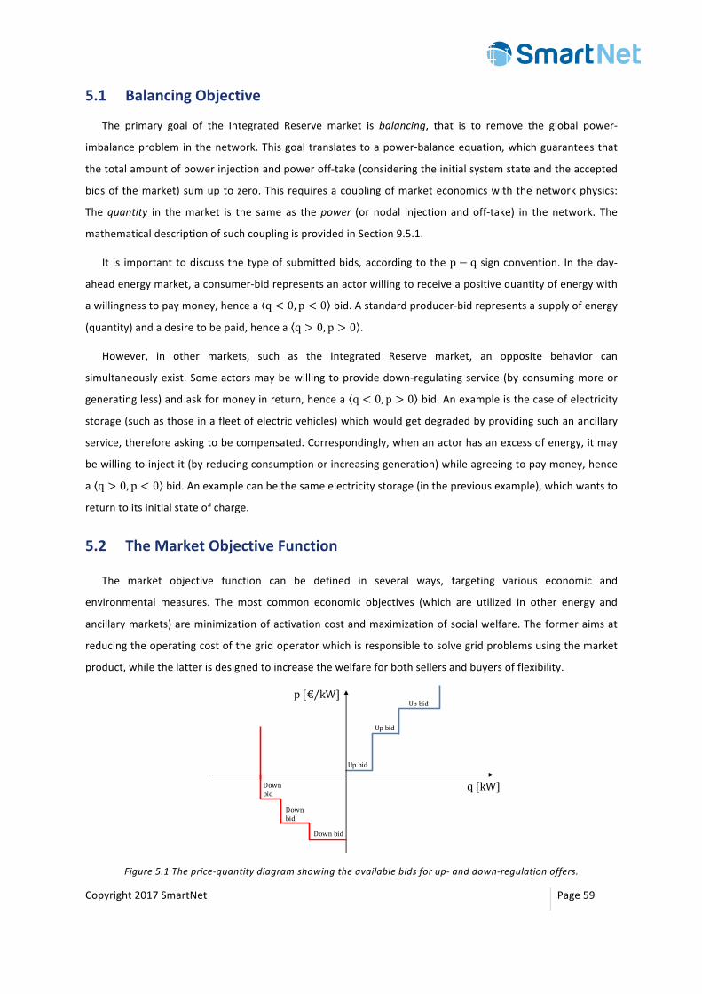
Copyright2017SmartNet Page59
5.1 BalancingObjective
The primary goal of the Integrated Reserve market is balancing, that is to remove the global power-
imbalanceprobleminthenetwork.Thisgoaltranslatestoapower-balanceequation,whichguaranteesthat
thetotalamountofpowerinjectionandpoweroff-take(consideringtheinitialsystemstateandtheaccepted
bidsofthemarket)sumuptozero.Thisrequiresacouplingofmarketeconomicswiththenetworkphysics:
Thequantity in themarket is the same as thepower (or nodal injection and off-take) in the network. The
mathematicaldescriptionofsuchcouplingisprovidedinSection9.5.1.
It is important todiscuss thetypeofsubmittedbids,accordingtothep − q signconvention. In theday-
aheadenergymarket,aconsumer-bidrepresentsanactorwillingtoreceiveapositivequantityofenergywith
awillingnesstopaymoney,hencea q < 0, p < 0 bid.Astandardproducer-bidrepresentsasupplyofenergy
(quantity)andadesiretobepaid,hencea q > 0, p > 0 .
However, in other markets, such as the Integrated Reserve market, an opposite behavior can
simultaneouslyexist.Someactorsmaybewillingtoprovidedown-regulatingservice(byconsumingmoreor
generatingless)andaskformoneyinreturn,hencea q < 0, p > 0 bid.Anexampleisthecaseofelectricity
storage(suchasthoseinafleetofelectricvehicles)whichwouldgetdegradedbyprovidingsuchanancillary
service,thereforeaskingtobecompensated.Correspondingly,whenanactorhasanexcessofenergy,itmay
bewillingtoinjectit(byreducingconsumptionorincreasinggeneration)whileagreeingtopaymoney,hence
a q > 0, p < 0 bid.Anexamplecanbethesameelectricitystorage(inthepreviousexample),whichwantsto
returntoitsinitialstateofcharge.
5.2 TheMarketObjectiveFunction
The market objective function can be defined in several ways, targeting various economic and
environmental measures. The most common economic objectives (which are utilized in other energy and
ancillarymarkets)areminimizationofactivationcostandmaximizationofsocialwelfare.Theformeraimsat
reducingtheoperatingcostofthegridoperatorwhichisresponsibletosolvegridproblemsusingthemarket
product,whilethelatterisdesignedtoincreasethewelfareforbothsellersandbuyersofflexibility.
Figure5.1Theprice-quantitydiagramshowingtheavailablebidsforup-anddown-regulationoffers.
p[€/kW]
q[kW]
Upbid
Upbid
Upbid
Downbid
Downbid
Downbid
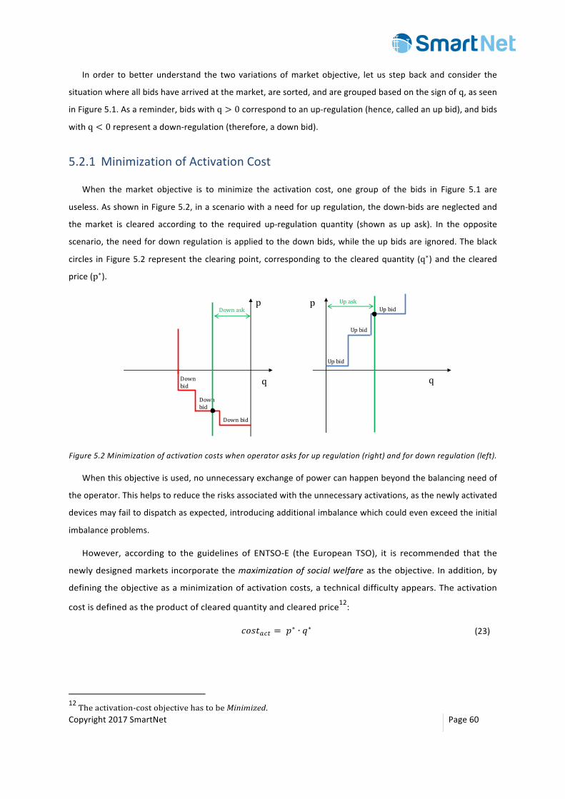
Copyright2017SmartNet Page60
In order to better understand the two variations ofmarket objective, let us stepback and consider the
situationwhereallbidshavearrivedatthemarket,aresorted,andaregroupedbasedonthesignofq,asseen
inFigure5.1.Asareminder,bidswithq > 0correspondtoanup-regulation(hence,calledanupbid),andbids
withq < 0representadown-regulation(therefore,adownbid).
5.2.1 MinimizationofActivationCost
When the market objective is to minimize the activation cost, one group of the bids in Figure 5.1 are
useless.AsshowninFigure5.2,inascenariowithaneedforupregulation,thedown-bidsareneglectedand
themarket is cleared according to the required up-regulation quantity (shown as up ask). In the opposite
scenario,theneedfordownregulationisappliedtothedownbids,whiletheupbidsareignored.Theblack
circles inFigure5.2 represent theclearingpoint,corresponding to theclearedquantity (q∗)andthecleared
price(p∗).
Figure5.2Minimizationofactivationcostswhenoperatorasksforupregulation(right)andfordownregulation(left).
Whenthisobjectiveisused,nounnecessaryexchangeofpowercanhappenbeyondthebalancingneedof
theoperator.Thishelpstoreducetherisksassociatedwiththeunnecessaryactivations,asthenewlyactivated
devicesmayfailtodispatchasexpected,introducingadditionalimbalancewhichcouldevenexceedtheinitial
imbalanceproblems.
However, according to the guidelines of ENTSO-E (the European TSO), it is recommended that the
newlydesignedmarketsincorporatethemaximizationofsocialwelfareastheobjective.Inaddition,by
definingtheobjectiveasaminimizationofactivationcosts,atechnicaldifficultyappears.Theactivation
costisdefinedastheproductofclearedquantityandclearedprice12:
𝑐𝑜𝑠𝑡+�l = 𝑝∗ ∙ 𝑞∗ (23)
12Theactivation-costobjectivehastobeMinimized.
p
q
Downbid
Downbid
Downbid
Downaskp
q
Upbid
Upbid
Upbid
Upask
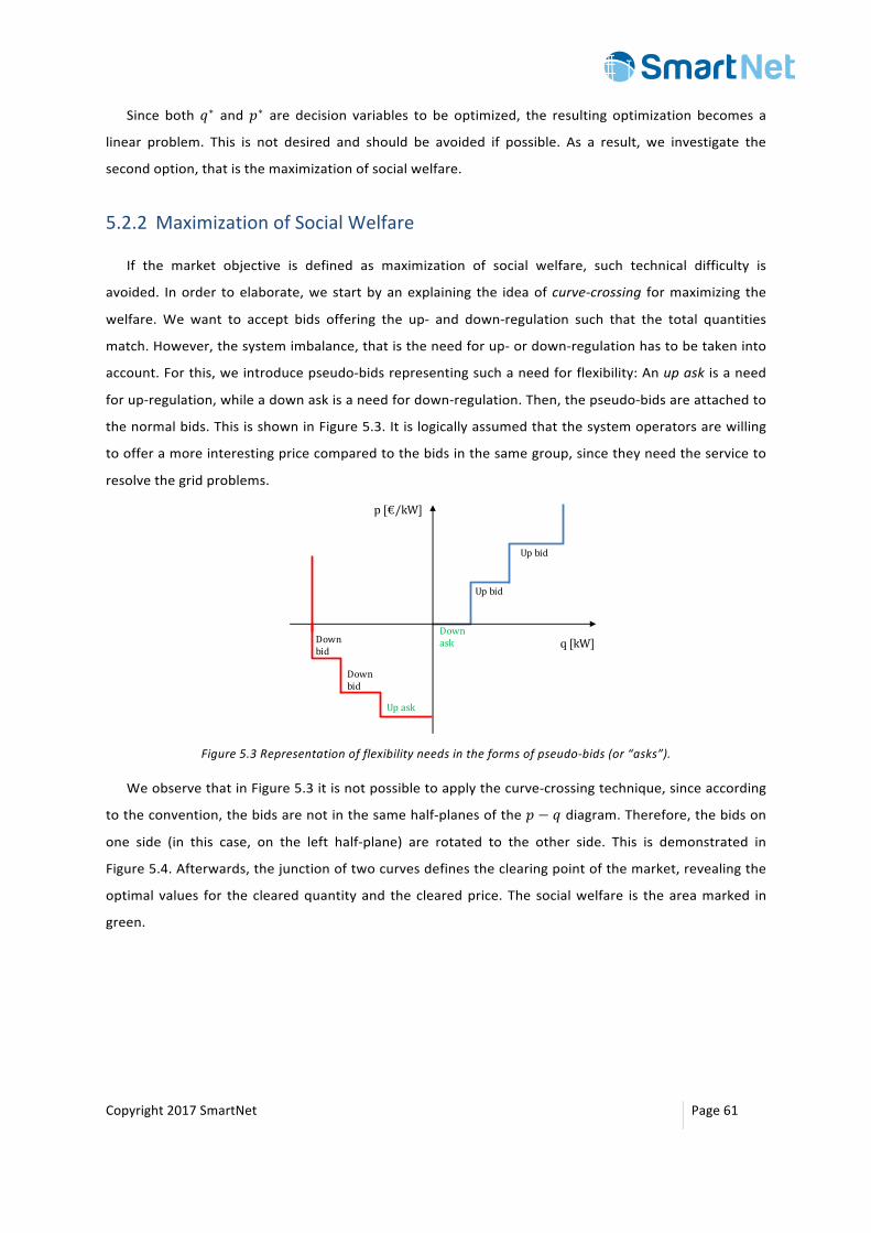
Copyright2017SmartNet Page61
Since both𝑞∗ and𝑝∗ are decision variables to be optimized, the resulting optimization becomes a
linear problem. This is not desired and should be avoided if possible. As a result, we investigate the
secondoption,thatisthemaximizationofsocialwelfare.
5.2.2 MaximizationofSocialWelfare
If the market objective is defined as maximization of social welfare, such technical difficulty is
avoided. Inorder toelaborate,we startbyanexplaining the ideaofcurve-crossing formaximizing the
welfare.We want to accept bids offering the up- and down-regulation such that the total quantities
match.However,thesystemimbalance,thatistheneedforup-ordown-regulationhastobetakeninto
account.Forthis,weintroducepseudo-bidsrepresentingsuchaneedforflexibility:Anupask isaneed
forup-regulation,whileadownaskisaneedfordown-regulation.Then,thepseudo-bidsareattachedto
thenormalbids.ThisisshowninFigure5.3.Itislogicallyassumedthatthesystemoperatorsarewilling
toofferamoreinterestingpricecomparedtothebidsinthesamegroup,sincetheyneedtheserviceto
resolvethegridproblems.
Figure5.3Representationofflexibilityneedsintheformsofpseudo-bids(or“asks”).
WeobservethatinFigure5.3itisnotpossibletoapplythecurve-crossingtechnique,sinceaccording
totheconvention,thebidsarenotinthesamehalf-planesofthe𝑝 − 𝑞diagram.Therefore,thebidson
one side (in this case, on the left half-plane) are rotated to the other side. This is demonstrated in
Figure5.4.Afterwards,thejunctionoftwocurvesdefinestheclearingpointofthemarket,revealingthe
optimal values for theclearedquantityand theclearedprice.The socialwelfare is theareamarked in
green.
p[€/kW]
q[kW]
Upbid
Upbid
Downask
Upask
Downbid
Downbid
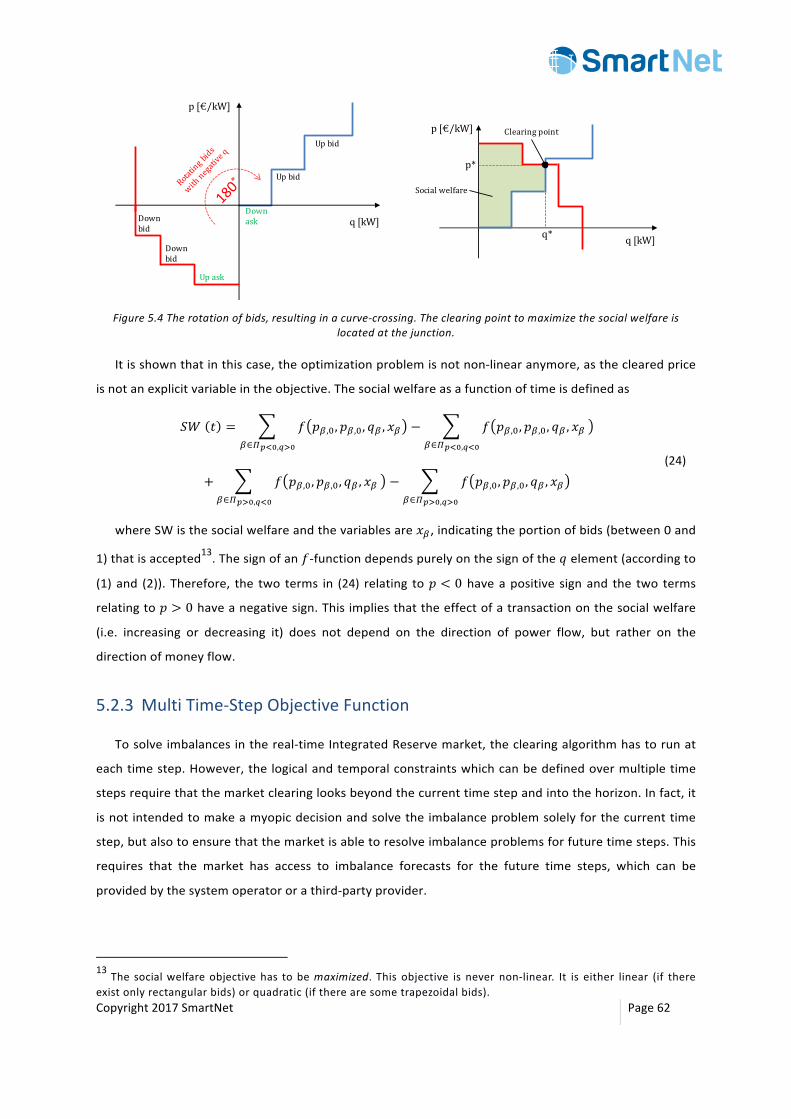
Copyright2017SmartNet Page62
Figure5.4Therotationofbids,resultinginacurve-crossing.Theclearingpointtomaximizethesocialwelfareis
locatedatthejunction.
Itisshownthatinthiscase,theoptimizationproblemisnotnon-linearanymore,astheclearedprice
isnotanexplicitvariableintheobjective.Thesocialwelfareasafunctionoftimeisdefinedas
𝑆𝑊 𝑡 = 𝑓 𝑝�,3, 𝑝�,3, 𝑞�, 𝑥��∈����,���
− 𝑓 𝑝�,3, 𝑝�,3, 𝑞�, 𝑥��∈����,���
+ 𝑓 𝑝�,3, 𝑝�,3, 𝑞�, 𝑥��∈����,���
− 𝑓 𝑝�,3, 𝑝�,3, 𝑞�, 𝑥��∈����,���
(24)
whereSWisthesocialwelfareandthevariablesare𝑥� ,indicatingtheportionofbids(between0and
1)thatisaccepted13.Thesignofan𝑓-functiondependspurelyonthesignofthe𝑞element(accordingto
(1)and (2)). Therefore, the two terms in (24) relating to𝑝 < 0haveapositive signand the two terms
relatingto𝑝 > 0haveanegativesign.Thisimpliesthattheeffectofatransactiononthesocialwelfare
(i.e. increasing or decreasing it) does not depend on the direction of power flow, but rather on the
directionofmoneyflow.
5.2.3 MultiTime-StepObjectiveFunction
Tosolveimbalancesinthereal-timeIntegratedReservemarket,theclearingalgorithmhastorunat
eachtimestep.However,thelogicalandtemporalconstraintswhichcanbedefinedovermultipletime
stepsrequirethatthemarketclearinglooksbeyondthecurrenttimestepandintothehorizon.Infact,it
isnotintendedtomakeamyopicdecisionandsolvetheimbalanceproblemsolelyforthecurrenttime
step,butalsotoensurethatthemarketisabletoresolveimbalanceproblemsforfuturetimesteps.This
requires that the market has access to imbalance forecasts for the future time steps, which can be
providedbythesystemoperatororathird-partyprovider.
13The socialwelfareobjectivehas tobemaximized. This objective is never non-linear. It is either linear (if thereexistonlyrectangularbids)orquadratic(iftherearesometrapezoidalbids).
p[€/kW]
q[kW]
Upbid
Upbid
Downask
Upask
Downbid
Downbid
p[€/kW]
q[kW]
Socialwelfare
Clearingpoint
q*
p*
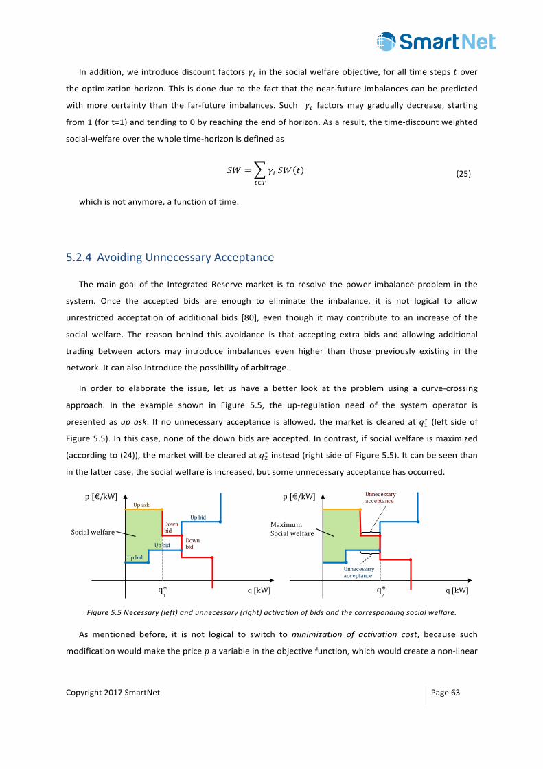
Copyright2017SmartNet Page63
Inaddition,weintroducediscountfactors𝛾l inthesocialwelfareobjective,foralltimesteps𝑡over
theoptimizationhorizon.This isdoneduetothefactthatthenear-futureimbalancescanbepredicted
withmore certainty than the far-future imbalances. Such 𝛾l factorsmay gradually decrease, starting
from1(fort=1)andtendingto0byreachingtheendofhorizon.Asaresult,thetime-discountweighted
social-welfareoverthewholetime-horizonisdefinedas
𝑆𝑊 = 𝛾ll∈�
𝑆𝑊 𝑡 (25)
whichisnotanymore,afunctionoftime.
5.2.4 AvoidingUnnecessaryAcceptance
Themain goal of the IntegratedReservemarket is to resolve the power-imbalance problem in the
system. Once the accepted bids are enough to eliminate the imbalance, it is not logical to allow
unrestricted acceptation of additional bids [80], even though it may contribute to an increase of the
social welfare. The reason behind this avoidance is that accepting extra bids and allowing additional
trading between actors may introduce imbalances even higher than those previously existing in the
network.Itcanalsointroducethepossibilityofarbitrage.
In order to elaborate the issue, let us have a better look at the problem using a curve-crossing
approach. In the example shown in Figure 5.5, the up-regulation need of the system operator is
presentedasupask. If nounnecessary acceptance is allowed, themarket is clearedat𝑞4∗ (left sideof
Figure5.5). Inthiscase,noneofthedownbidsareaccepted. Incontrast, ifsocialwelfare ismaximized
(accordingto(24)),themarketwillbeclearedat𝑞E∗ instead(rightsideofFigure5.5).Itcanbeseenthan
inthelattercase,thesocialwelfareisincreased,butsomeunnecessaryacceptancehasoccurred.
Figure5.5Necessary(left)andunnecessary(right)activationofbidsandthecorrespondingsocialwelfare.
As mentioned before, it is not logical to switch tominimization of activation cost, because such
modificationwouldmaketheprice𝑝avariableintheobjectivefunction,whichwouldcreateanon-linear
p[€/kW]
q[kW]q*2
Unnecessaryacceptance
Unnecessaryacceptance
MaximumSocialwelfare
Downbid
p[€/kW]
q[kW]q*
Upask
UpbidUpbid
Upbid
Downbid
1
Socialwelfare
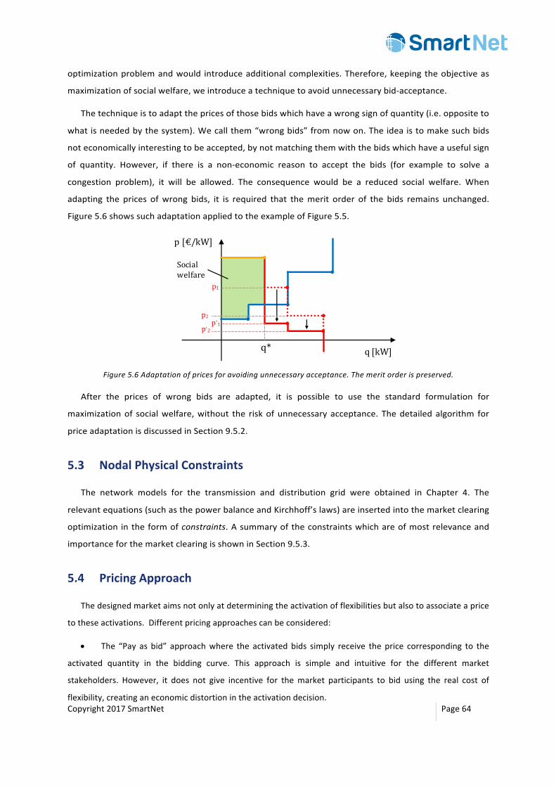
Copyright2017SmartNet Page64
optimizationproblemandwould introduceadditionalcomplexities.Therefore,keepingtheobjectiveas
maximizationofsocialwelfare,weintroduceatechniquetoavoidunnecessarybid-acceptance.
Thetechniqueistoadaptthepricesofthosebidswhichhaveawrongsignofquantity(i.e.oppositeto
whatisneededbythesystem).Wecallthem“wrongbids”fromnowon.Theideaistomakesuchbids
noteconomicallyinterestingtobeaccepted,bynotmatchingthemwiththebidswhichhaveausefulsign
of quantity. However, if there is a non-economic reason to accept the bids (for example to solve a
congestion problem), it will be allowed. The consequence would be a reduced social welfare. When
adapting the prices ofwrong bids, it is required that themerit order of the bids remains unchanged.
Figure5.6showssuchadaptationappliedtotheexampleofFigure5.5.
Figure5.6Adaptationofpricesforavoidingunnecessaryacceptance.Themeritorderispreserved.
After the prices of wrong bids are adapted, it is possible to use the standard formulation for
maximizationof socialwelfare,without the riskofunnecessaryacceptance. Thedetailedalgorithm for
priceadaptationisdiscussedinSection9.5.2.
5.3 NodalPhysicalConstraints
The network models for the transmission and distribution grid were obtained in Chapter 4. The
relevantequations(suchasthepowerbalanceandKirchhoff’slaws)areinsertedintothemarketclearing
optimization intheformofconstraints.Asummaryoftheconstraintswhichareofmostrelevanceand
importanceforthemarketclearingisshowninSection9.5.3.
5.4 PricingApproach
Thedesignedmarketaimsnotonlyatdeterminingtheactivationofflexibilitiesbutalsotoassociateaprice
totheseactivations.Differentpricingapproachescanbeconsidered:
• The “Pay as bid” approachwhere the activated bids simply receive the price corresponding to the
activated quantity in the bidding curve. This approach is simple and intuitive for the different market
stakeholders. However, it does not give incentive for themarket participants to bid using the real cost of
flexibility,creatinganeconomicdistortionintheactivationdecision.
p[€/kW]
q[kW]q*
Socialwelfare
p1
p2p'2p'1

Copyright2017SmartNet Page65
• The“Payascleared”or“locationalmarginalprice(LMP)approach”wheretheactivatedbidsreceive
the same price per MWh (or MW over a time step), corresponding to the most expensive (or the least
economicallyinteresting)activatedflexibility.Thisapproachremovestheriskofmarketparticipantbiddingin
termsofwhattheywanttoreceiveinsteadoftheirrealcostofflexibility.
Asthemotivationofthedesignedmarketistoallowafairandcost-efficientcompetitionbetweendifferent
sourcesofflexibilities, inparticularthoselocatedatthedistributionlevel, itappearsnaturaltousethemost
economicallyefficientapproachofthemarginalpricing[81].
However, as the considered system is not a perfect copper plate, network constraints, both at the
transmissionanddistributionlevels,havetobetakenintoaccount.
Marginalpricingcanbeadaptedtoasystemwithnetworkconstraintsindifferentways:
• ANodalapproachwhereapriceforflexibilityisassociatedtothemostgranularlevelinournetwork
representationi.e.toeachnodeofthedistributiongrid
• AZonalapproachwhereapricefor flexibility isassociatedtoazonecoveringdifferentnodes.Each
zonecanhaveadifferentpricebutthenodesinthesamezonehavethesameprice.
Asthenetworkconstraints,bothatthetransmissionanddistributionlevels,areofkeyimportanceforan
ancillary service market ensuring the satisfaction of congestion and voltage constraints, it is natural to
encompassinthepricemechanismthesenetworkfactorsinthemostaccurateandeconomicallyefficientway.
Moreover,ancillaryservicemarketsareclose-to-real-timemarketandtheirdecisionscannotbecorrectedbya
market afterwards. For these reasons, a nodal approach is proposed for the considered Integrated Reserve
markettobedesigned.Further justificationsandthederivationofthedistributionlocationalmarginalprices
fortheconsiderednetworkmodelanditsinterpretationisdetailedintherestofthechapter.
5.5 NodalMarginalPricing
Thetheoryofnodalmarginalpricingispredicatedonthemoregeneraleconomicconceptofmarginal
costpricing,whichisanapproachthatachievesanefficientallocationofresourcesundertheassumption
ofperfect competition.The ideaofmarginal costpricing is simple,anddictates thatconsumerswitha
well-definedwillingness to pay for a commodity should consume as long as their incremental benefit
exceeds the incremental cost of the additional production. In an economy where consumers can be
stackedinorderofdecreasingvaluationandsupplierscanbestackedinorderofincreasingmarginalcost
itiseasytoseewhythissystemallocatesresourcesefficiently:consumerswiththehighestwillingnessto
payarematchedwithsupplierswiththe lowestmarginalcostofproduction,uptothepointwhereno
additionalmutualbenefitsfromtradecanbeachieved.Inordertorespectcompatibilitywithourmarket,
oneshouldinterpreta“consumerbid”asabidwith𝑝 < 0anda“supplierbid”asonewith𝑝 > 0.
Copyright2017SmartNet Page66
5.5.1 PricingoverSpaceandTime
The complicating factor of electric power systems is the fact thatmarginal cost cannot be defined
uniformly for all locations, or for a single time period, but instead depends on the configuration of
demand over the network and the availability and physical characteristics of power generation,
transmissionanddistributionequipment,andchangescontinuously(overminutes,hours,days,…).This
ledtothetheoryofspotpricingofelectricityoverspaceandtime,championedbytheseminalworkof
Schweppe,Caramanis,andTabors[82],[83].
Amajorreasonwhymarginalcostcannotbedefineduniformlyforalllocationsofapowersystemis
the physical laws that govern power flow, losses, and limits on transmission and distribution lines. A
numericalexampleisshowninSection9.5.4.
5.5.2 Granularity
There has been a longstanding debate about the granularity of pricing in electricitymarkets.More
specifically,nodalpricinghasbeencriticizedforthinningupmarketsandcreatingopportunities forthe
exerciseofmarketpower,aswellas forcreatingapricingsystemthat is toocomplexorunnecessarily
granular.Successfulexperienceofnodalpricinginsomeofthelargestmarketsworldwide,includingthe
PennsylvaniaJerseyMaryland(PJM)marketwhichprices8700locationswithafrequencyof15minutes,
have discarded concerns of complexity. Market power mitigation by market monitors has further
softenedconcernsregardingtheexerciseofmarketpower.
Analternativetonodalpricingthathasbeenadvocatedonthegroundsofsimplicityiszonalpricing,
whereby nodes are aggregated into zoneswith a commonprice (which implicitly assumes away intra-
zonal congestion) and inter-zonal lines are aggregated into a single link. This aggregation creates a
challengeofdefiningcapacityandcreatingaproxyfortherepresentationofpowerflowlaws,asshown
in a numerical example in Section 9.5.5. The conclusion is that a zonal model will either sacrifice
efficiencyorwelfare,sinceitignoresthephysicallawsthatgovernpowerflow.Remediestothisissueby
meansof re-dispatchinghaveexposedthemarket toseveregamingopportunities (including theEnron
“Decgame”)[84],resultinday-aheadschedulinginefficiencies[85],andcreatefree-ridingopportunities
forcertainzonesonthetransmissiongridsofotherzones[86].
5.6 CalculatingPrices
Thestandarddefinitionofmarketequilibriumineconomicsisapairofpricesandquantitiessuchthat,
given the prices, agents maximize profits, and prices are such that supply and demand are equal. It
follows from standard results in convex optimization that this definition ofmarket equilibrium implies
thatthepriceofelectricalpowerintheoptimalpowerflowproblemcanbeobtainedasthedualoptimal

Copyright2017SmartNet Page67
multiplier of thepowerbalance constraints14. Theseprices canbeobtainedby solving thedual of the
optimalpowerflowproblem,whichisformulatedasasetofconstraintsinthemarketclearingalgorithm.
Therefore,theclearingofquantitiesiscalledthe“primaryproblem”,andtheclearingofnodalmarginal
pricesisreferredtoasthe“dualproblem”.
Awide rangeofoptimizationalgorithms that areused in commercial applications for solving linear
programs, second-order coneprograms, andmoregenerallynon-linearprograms, solve thedual of an
optimizationproblemasaby-productofsolvingtheprimalproblem.Thisimpliesthat,inordertoobtain
prices,itisnotnecessarytosolvethedualproblemexplicitly,sincethisisanywaysaside-productofthe
optimization process. Commercial solvers (such as CPLEX) will then typically furnish primal optimal
variablesthatareusedfordecidinghowtodispatchanasset,howmuchpowershouldflowoveraline,
whatthevoltageofanodeis,aswellaspricesthatshouldbeassignedtoanexchangeofquantity.
5.6.1 NodalClearedPricesasDualVariables
The nodal dual variable associatedwith the nodal power-balance constraint (see (216)) equals the
marginal price of injecting/off-taking one unit of power in that node. In principle, for a linear
programming(LP)problem,theclearedpricep∗canbefetchedbyrequestingtheLP-solvertoprovidethe
valueofthedualvariable.
In reality, themarket clearing problem contains binary variables. In such a case, the clearedprices
need tobederivedusing adedicatedalgorithm. Theprice is not explicitlypresent as a variable in the
model of the primal problem; if it was, the primal problem would belong to a category of problems
knownasMathematicalProblemswithEquilibriumConstraints (MPEC),whichareknowntobehardto
solve since their feasible region is not necessarily convex or connected [87]. Further explanation is
providedinSection9.5.6.
Byavoidingthesituationofhavingpricesasexplicitvariablesintheprimalproblem,suchdifficultyis
avoided.Italsomeansthatthedualproblemdoesnothavetobesolvedexplicitly,exceptinthecaseof
indeterminaciesorparadoxicalacceptance.
In general, indeterminacies can happen for both quantity and price. Figure 5.7 compares the
situationswithnoindeterminaciesandthosewithindeterminacies.Incaseofaquantityindeterminacy,
the rule of volumemaximization applies, resulting in the selection of clearing point at the end of the
horizontalcrosssection. Incaseofaprice indeterminacy, therule is tochoosethemiddlepointof the
verticalcrosssection.Section9.5.7explainsthealgorithminmoredetailsusinganumericalexample.
14 This statement is true for convex problems. Problems with binary decision variables pose deeper theoreticalquestionsofdefiningwhatamarketclearedpriceis,asdiscussedinthenextsection.
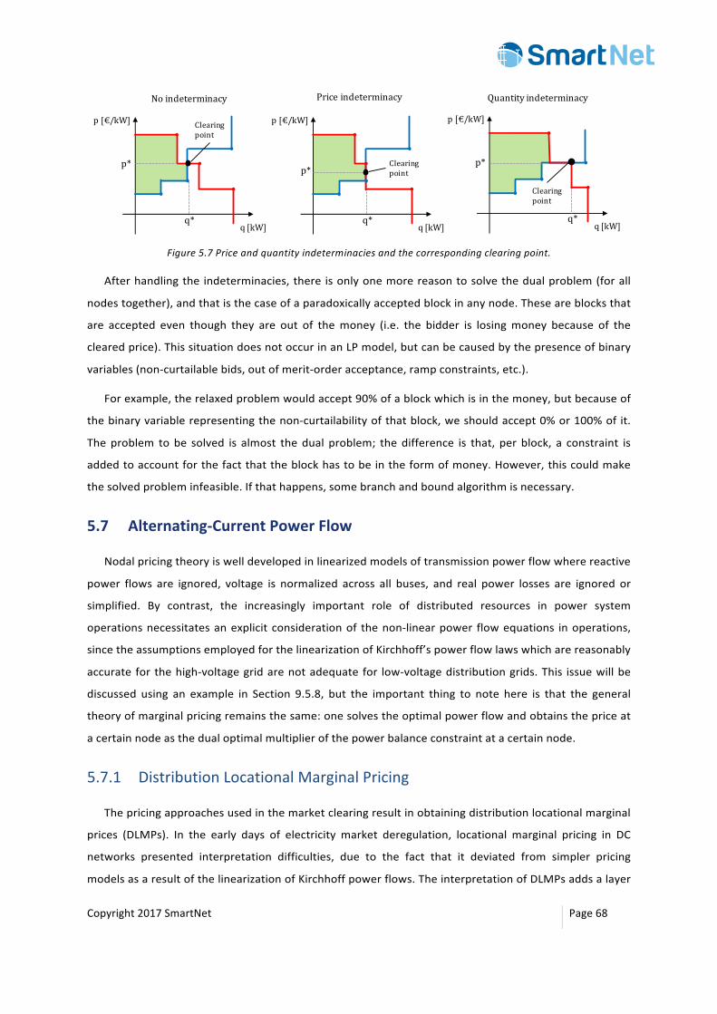
Copyright2017SmartNet Page68
Figure5.7Priceandquantityindeterminaciesandthecorrespondingclearingpoint.
Afterhandlingthe indeterminacies,there isonlyonemorereasontosolvethedualproblem(forall
nodestogether),andthatisthecaseofaparadoxicallyacceptedblockinanynode.Theseareblocksthat
are accepted even though they are out of themoney (i.e. the bidder is losingmoney because of the
clearedprice).ThissituationdoesnotoccurinanLPmodel,butcanbecausedbythepresenceofbinary
variables(non-curtailablebids,outofmerit-orderacceptance,rampconstraints,etc.).
Forexample,therelaxedproblemwouldaccept90%ofablockwhichisinthemoney,butbecauseof
thebinaryvariablerepresentingthenon-curtailabilityofthatblock,weshouldaccept0%or100%ofit.
Theproblem tobe solved is almost thedual problem; thedifference is that, per block, a constraint is
addedtoaccountforthefactthattheblockhastobeintheformofmoney.However,thiscouldmake
thesolvedprobleminfeasible.Ifthathappens,somebranchandboundalgorithmisnecessary.
5.7 Alternating-CurrentPowerFlow
Nodalpricingtheoryiswelldevelopedinlinearizedmodelsoftransmissionpowerflowwherereactive
power flows are ignored, voltage is normalized across all buses, and real power losses are ignored or
simplified. By contrast, the increasingly important role of distributed resources in power system
operationsnecessitatesanexplicit considerationof thenon-linearpower flowequations inoperations,
sincetheassumptionsemployedforthelinearizationofKirchhoff’spowerflowlawswhicharereasonably
accurateforthehigh-voltagegridarenotadequatefor low-voltagedistributiongrids.This issuewillbe
discussed using an example in Section 9.5.8, but the important thing to note here is that the general
theoryofmarginalpricingremainsthesame:onesolvestheoptimalpowerflowandobtainsthepriceat
acertainnodeasthedualoptimalmultiplierofthepowerbalanceconstraintatacertainnode.
5.7.1 DistributionLocationalMarginalPricing
Thepricingapproachesusedinthemarketclearingresultinobtainingdistributionlocationalmarginal
prices (DLMPs). In the early days of electricity market deregulation, locational marginal pricing in DC
networks presented interpretation difficulties, due to the fact that it deviated from simpler pricing
modelsasaresultofthelinearizationofKirchhoffpowerflows.TheinterpretationofDLMPsaddsalayer
Noindeterminacy
p[€/kW]
q[kW]q*
Clearingpoint
p*
Priceindeterminacy
p[€/kW]
q[kW]q*
Clearingpointp*
Quantityindeterminacy
p[€/kW]
q[kW]q*
Clearingpoint
p*

Copyright2017SmartNet Page69
of complexity, since voltage, real power losses, and reactive power flows are accounted for, whereas
theseaspectsoftheproblemareeithersimplifiedorignoredinDCpowerflow.Variousmethodscanbe
usedforunderstandingandinterpretingthevalueofDLMPs,withtheobjectiveof justifyingtheirvalue
onphysicalgrounds.InSection9.5.9weshowthreedifferentapproachestoanswerthequestionofwhy
DLMPsobtainthespecificvaluefurnishedbythemarketclearingalgorithm.
5.8 MarketClearingAlgorithm
The clearing algorithm is an optimization problem which is solved at every time step. Here we
summarize the comprising routines. The following multi time-step clearing algorithm over the time
horizonissetup:
1. Initialization:Settheparametersandinitialvalues(basedontheoutputoftheoldmarketclearings);
2. Bidacquisition:Receivebidsandprocessthemtocreateprimitivebids;
3. Networkmodeling:Receivethenetworkstate(forexamplethepower injectionateachnode)and
lineparameters,thencalculatethetotalsystemimbalanceandidentifycongestionproblems;
4. Problemformulation:Createtheobjectivefunctionandeconomicandphysicalconstraints;
5. Clearing:Solvetheoptimizationproblemandfindtheclearedquantityandclearednodalprices;
6. Finalization:Transmittheinformationregardingclearedbids;
7. Waituntilthenexttimestepandreturntostep1.
Themarketresolution(i.e. lengthofatimestep), thetimehorizon,andthefrequencyatwhichthe
optimizationisrunning,aredesignparametersthatcanbeadjustedattheimplementationstage.
Copyright2017SmartNet Page70
6 TSO-DSOCoordinationSchemes
Previous sections have focused on describing the mathematical formulations needed to clear a
market: market products specification, simplified network model, clearing algorithm, and pricing
mechanism.
Inthecentralizedapproach,wheretheDSOhasnolocalmarket, it istheTSO(orthemarketoperator in
general) who takes the activation decisions for flexibilities proposed, not only at the transmission network
level,butalsoatthelevelofthedistributionnetworks.
Twodifferentvariantsofthiscentralizedmodelcanbeconsidered:
• Full-observabilityvariant:Inthisapproach,theTSOclearstheglobalbalancingmarketbytakinginto
account congestions using (simplified) models of the transmission network, but also of the different
distributionnetworks.
• No-observabilityfromTSO:TheTSOclearstheglobalancillaryservices(IntegratedReserve)market
withoutexplicitlytaking intoaccountthemodelsofthedistributionnetworks. It ispossibletoconsidersuch
network constraints, butmore computation timewill be required.Ablocking/vetoprocess from theDSO is
thereforeneededafterthemarketclearingduringthecounter-tradingphase.Themarketclearingwillnotrun
again,butratherthecounter-tradingishandledoutsidethemarket,withalimitedtimeallowedforvetoes.In
caseofaveto, theTSO (or theDSO)canuse itsownresources tocompensate for theassetswhicharenot
activated.
Inthischapter,wedescribethespecificitiesandrequirementsofthemarketarchitecturesforthedifferent
TSO-DSOcoordinationschemesinvestigatedintheSmartNetproject[1].
6.1 CentralizedvsDecentralizedMarketArchitectures
Firstofall,animportantdifferencebetweenTSO-DSOcoordinationschemesiswhetheracentralized
ordecentralizedarchitecture(seeFigure6.1)isconsidered.Table6.1showswhicharchitectureisusedin
eachcoordinationscheme.
Centralizedarchitecture DecentralizedmarketarchitectureCentralizedASmarket LocalASmarketCommonTSO-DSOASmarket(centralized) CommonTSO-DSOASmarket(decentralized)Integratedflexibilitymarket Sharedbalancingresponsibilitymodel
Table6.1Listofcentralizedanddecentralizedarchitectures.
Inthecentralizedarchitecture,there isone(big)market,whilefordecentralizedarchitecture,many
localmarkets(managedbyDSOs)co-existwithaglobalASmarket.Forthedecentralizedarchitecture,we
have:
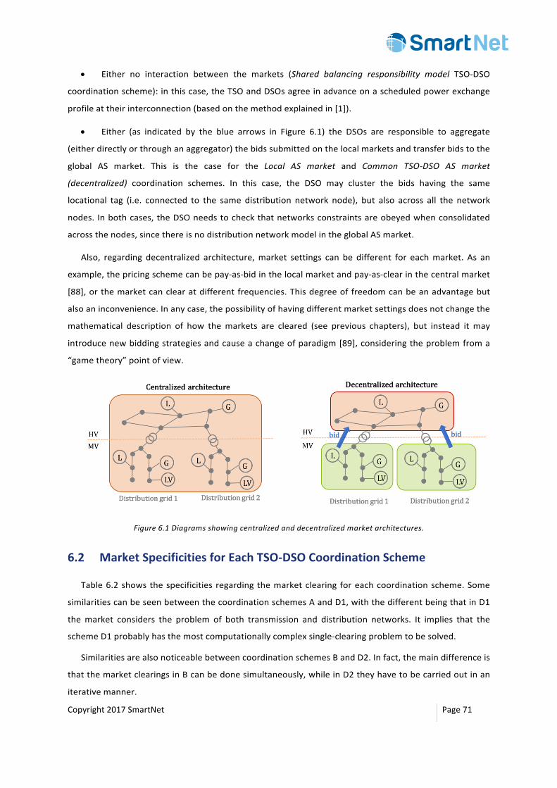
Copyright2017SmartNet Page71
• Either no interaction between the markets (Shared balancing responsibility model TSO-DSO
coordinationscheme):inthiscase,theTSOandDSOsagreeinadvanceonascheduledpowerexchange
profileattheirinterconnection(basedonthemethodexplainedin[1]).
• Either (as indicated by the blue arrows in Figure 6.1) the DSOs are responsible to aggregate
(eitherdirectlyorthroughanaggregator)thebidssubmittedonthelocalmarketsandtransferbidstothe
global AS market. This is the case for the Local AS market and Common TSO-DSO AS market
(decentralized) coordination schemes. In this case, the DSO may cluster the bids having the same
locational tag (i.e. connected to the same distribution network node), but also across all the network
nodes. Inbothcases,theDSOneedstocheckthatnetworksconstraintsareobeyedwhenconsolidated
acrossthenodes,sincethereisnodistributionnetworkmodelintheglobalASmarket.
Also, regarding decentralized architecture,market settings can be different for eachmarket. As an
example,thepricingschemecanbepay-as-bidinthelocalmarketandpay-as-clearinthecentralmarket
[88],orthemarketcanclearatdifferentfrequencies.Thisdegreeoffreedomcanbeanadvantagebut
alsoaninconvenience.Inanycase,thepossibilityofhavingdifferentmarketsettingsdoesnotchangethe
mathematical description of how themarkets are cleared (see previous chapters), but instead itmay
introducenewbiddingstrategiesandcauseachangeofparadigm[89],consideringtheproblemfroma
“gametheory”pointofview.
Figure6.1Diagramsshowingcentralizedanddecentralizedmarketarchitectures.
6.2 MarketSpecificitiesforEachTSO-DSOCoordinationScheme
Table6.2showsthespecificities regardingthemarketclearing foreachcoordinationscheme.Some
similaritiescanbeseenbetweenthecoordinationschemesAandD1,withthedifferentbeingthatinD1
themarket considers the problem of both transmission and distribution networks. It implies that the
schemeD1probablyhasthemostcomputationallycomplexsingle-clearingproblemtobesolved.
SimilaritiesarealsonoticeablebetweencoordinationschemesBandD2.Infact,themaindifferenceis
thatthemarketclearingsinBcanbedonesimultaneously,whileinD2theyhavetobecarriedoutinan
iterativemanner.
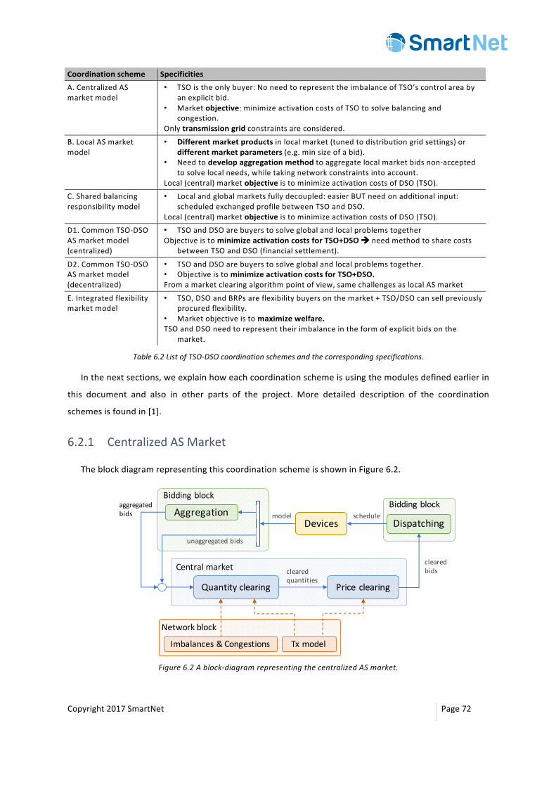
Copyright2017SmartNet Page72
Coordinationscheme SpecificitiesA.CentralizedASmarketmodel
• TSOistheonlybuyer:NoneedtorepresenttheimbalanceofTSO’scontrolareabyanexplicitbid.
• Marketobjective:minimizeactivationcostsofTSOtosolvebalancingandcongestion.
Onlytransmissiongridconstraintsareconsidered.
B.LocalASmarketmodel
• Differentmarketproductsinlocalmarket(tunedtodistributiongridsettings)ordifferentmarketparameters(e.g.minsizeofabid).
• Needtodevelopaggregationmethodtoaggregatelocalmarketbidsnon-acceptedtosolvelocalneeds,whiletakingnetworkconstraintsintoaccount.
Local(central)marketobjectiveistominimizeactivationcostsofDSO(TSO).C.Sharedbalancingresponsibilitymodel
• Localandglobalmarketsfullydecoupled:easierBUTneedonadditionalinput:scheduledexchangedprofilebetweenTSOandDSO.
Local(central)marketobjectiveistominimizeactivationcostsofDSO(TSO).D1.CommonTSO-DSOASmarketmodel(centralized)
• TSOandDSOarebuyerstosolveglobalandlocalproblemstogetherObjectiveistominimizeactivationcostsforTSO+DSOàneedmethodtosharecosts
betweenTSOandDSO(financialsettlement).
D2.CommonTSO-DSOASmarketmodel(decentralized)
• TSOandDSOarebuyerstosolveglobalandlocalproblemstogether.• ObjectiveistominimizeactivationcostsforTSO+DSO.Fromamarketclearingalgorithmpointofview,samechallengesaslocalASmarket
E.Integratedflexibilitymarketmodel
• TSO,DSOandBRPsareflexibilitybuyersonthemarket+TSO/DSOcansellpreviouslyprocuredflexibility.
• Marketobjectiveistomaximizewelfare.TSOandDSOneedtorepresenttheirimbalanceintheformofexplicitbidsonthe
market.
Table6.2ListofTSO-DSOcoordinationschemesandthecorrespondingspecifications.
Inthenextsections,weexplainhoweachcoordinationschemeisusingthemodulesdefinedearlierin
this document and also in other parts of the project. More detailed description of the coordination
schemesisfoundin[1].
6.2.1 CentralizedASMarket
TheblockdiagramrepresentingthiscoordinationschemeisshowninFigure6.2.
Figure6.2Ablock-diagramrepresentingthecentralizedASmarket.
BiddingblockBiddingblock
Centralmarket
PriceclearingQuantityclearing
aggregatedbids
DispatchingDevicesAggregation
unaggregatedbids
model schedule
clearedquantities
clearedbids
Networkblock
Imbalances&Congestions Txmodel
Copyright2017SmartNet Page73
Thediagramshowsasetofblocksrepresentingmodules,andarrowswhichcorrespondtodataflows.
Theblocksareconnectedsequentiallyinaclosedloop,implyingthattheprocedureisrepeatedateach
timestep.HereweprovideadescriptionofeachblockinFigure6.2:
• Devices:Thisblockincludesthemodelsofavailableflexibleassets inbothdistributionnetwork(Dx)
and transmission network (Tx). Input to this block is the dispatching schedule for the following time step.
Outputs from this block are themodels and parameters (including internal states) of flexible assets.More
informationaboutthecontentsofthisblockcanbefoundinD1.2[90].
• Bidding: This block contains the algorithms required for aggregation and dispatching (or
disaggregationplusconsideringthephysicallayer)offlexibledevices.Theaggregationmodulereceivesdevice
models and produces bids. The dispatching module receives the cleared bids and generates dispatching
schedulesforselectedflexibleassets.Moreinformationaboutthecontentsoftheseblockscanbefoundin[5].
• Network:Thisblockcontains thenetworkmodel, includingnetwork topology, lineconnectionsand
parameters, power-flows and voltage constraints, forecasts of system imbalance, etc. As described in
Chapter 4, different models are considered for distribution (Dx) and transmission (Tx) grids. In this
coordinationscheme,only theTxmodel is considered, since theDxproblemsarenot solved in themarket.
This model is used in the quantity and price clearing blocks, in order to locate the submitted bids and to
calculatethenodalprices.
• Market: This block represents the clearing processes regarding quantity and price, which are
thoroughlydiscussed inChapter5.Several typesofmarketsexist indifferentcoordinationschemes,suchas
local(DSO)market,central(TSO)market,andcommon(TSO-DSO)market.
6.2.2 LocalASMarket
TheblockdiagramrepresentingthiscoordinationschemeisshowninFigure6.3.Blocksareorganized
into four categories as in centralizedASmarket. However, alternative block connections and different
sequenceofrunningisusedinthiscase:
• Devices:Inthiscoordinationscheme,DxdevicesparticipateinthelocalmarketrunbyDSO(whileTx
devicesparticipateinthecentralmarketrunbyTSO).
• Bidding: Since devices connected directly to Tx are large, no aggregation is needed for them in
general.Also,separatedispatchingstepsareusedforDxandTxdevices.
• Network:Here,DxandTxmodelsareusedinthelocalandcentralmarket,respectively.Congestion
problems are treated by the corresponding network operators in both local and centralmarket. However,
imbalancesareonlyconsideredinthecentralmarket.

Copyright2017SmartNet Page74
Figure6.3Ablock-diagramrepresentingtheLocalASmarket.
• Market:ThecentralmarketblockisorganizedsimilartotheblocksincentralizedASmarket.Onthe
contrary, the local market block includes two additional components; DSO aggregation, and DSO
disaggregation.FirstDSOclearsafractionofbidstosolvethecongestionproblemsinDx.Then,theuncleared
bidsareprocessedbytheDSOaggregationblockwhichusesaparametricoptimization(oranotheralgorithm)
toconditionallyclearthebidsandtoaggregatethem.Thisstep is furtherexplainedinSection6.3.Afterthe
clearance of central market, the cleared DSO-bids return to the DSO disaggregation blocks, when the
previouslycalculatedparametersareusedtodeterminewhichnon-aggregatedbidshavetobelocallycleared.
6.2.3 SharedBalancingResponsibilityModel
TheblockdiagramrepresentingthiscoordinationschemeisshowninFigure6.4.Inthisscheme,DSO
andTSOsolvetheirowncongestionand imbalanceproblemsusingthedevicesconnectedtotheirown
networks.However,additionalconstraintsonDxandTxareusedtoscheduleprofilesofpowerexchange
betweenDx and Tx at connecting nodes. These profiles are generated prior to any optimization using
forecastsofpowerinjectionateachnodeofthenetwork.
Networkblock
Biddingblock
Biddingblock
Biddingblock
Biddingblock
Localmarket
PriceclearingQuantityclearing
Centralmarket
Txdevices
PriceClearing
aggregatedbids
QuantityClearing
ImbalancesCongestions Txmodel Dxmodel
AggregationDxdevices
unaggregatedbids
Dispatching
DSODisaggregation
Dispatchingmodel schedule
clearedquantities
clearedDSO-bids
unclearedquantities
aggregated bids(conditionallycleared)
Parameters
clearedTSO-bids
schedule
clearedaggregatedDSO-bids
unaggregatedTSO- bids
DSOAggregation(Parametricoptimization)
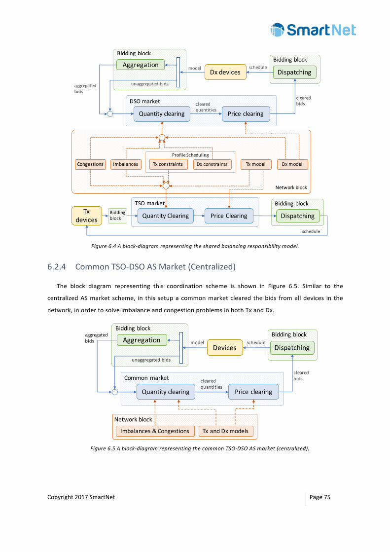
Copyright2017SmartNet Page75
Figure6.4Ablock-diagramrepresentingthesharedbalancingresponsibilitymodel.
6.2.4 CommonTSO-DSOASMarket(Centralized)
The block diagram representing this coordination scheme is shown in Figure 6.5. Similar to the
centralizedASmarket scheme, in this setupacommonmarketcleared thebids fromalldevices in the
network,inordertosolveimbalanceandcongestionproblemsinbothTxandDx.
Figure6.5Ablock-diagramrepresentingthecommonTSO-DSOASmarket(centralized).
Biddingblock
Biddingblock
Biddingblock
Networkblock
DSOmarket
Aggregation
Priceclearing
Dxdevices
Quantityclearing
TSOmarketTx
devices PriceClearingQuantityClearing
ProfileScheduling
ImbalancesCongestions DxconstraintsTxconstraints
unaggregatedbidsaggregatedbids
Txmodel Dxmodel
Dispatching
Dispatching
Biddingblock
model schedule
schedule
clearedquantities
clearedbids
BiddingblockBiddingblock
Commonmarket
Priceclearing
aggregatedbids
DispatchingDevicesAggregation
unaggregatedbids
model schedule
clearedquantities
clearedbids
Networkblock
Imbalances&Congestions TxandDxmodels
Quantityclearing
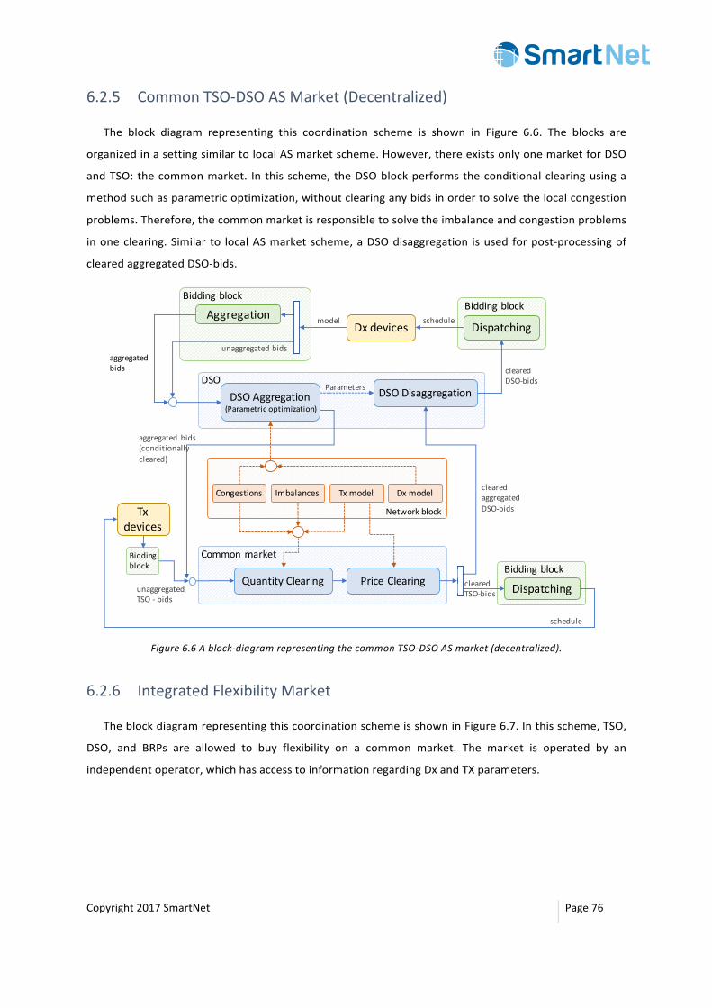
Copyright2017SmartNet Page76
6.2.5 CommonTSO-DSOASMarket(Decentralized)
The block diagram representing this coordination scheme is shown in Figure 6.6. The blocks are
organizedinasettingsimilartolocalASmarketscheme.However,thereexistsonlyonemarketforDSO
andTSO:thecommonmarket. Inthisscheme,theDSOblockperformstheconditionalclearingusinga
methodsuchasparametricoptimization,withoutclearinganybidsinordertosolvethelocalcongestion
problems.Therefore,thecommonmarketisresponsibletosolvetheimbalanceandcongestionproblems
inoneclearing.Similar to localASmarketscheme,aDSOdisaggregation isused forpost-processingof
clearedaggregatedDSO-bids.
Figure6.6Ablock-diagramrepresentingthecommonTSO-DSOASmarket(decentralized).
6.2.6 IntegratedFlexibilityMarket
TheblockdiagramrepresentingthiscoordinationschemeisshowninFigure6.7.Inthisscheme,TSO,
DSO, and BRPs are allowed to buy flexibility on a common market. The market is operated by an
independentoperator,whichhasaccesstoinformationregardingDxandTXparameters.
DSO
Biddingblock
BiddingblockBiddingblock
Commonmarket
PriceClearing
aggregatedbids
Remainingbids
QuantityClearing
Networkblock
ImbalancesCongestions Txmodel Dxmodel
AggregationDispatchingDxdevices
unaggregatedbids
Dispatching
DSODisaggregation
aggregated bids(conditionallycleared)
clearedDSO-bids
clearedTSO-bids
clearedaggregatedDSO-bids
Biddingblock
Txdevices
unaggregatedTSO- bids
schedule
model schedule
ParametersDSOAggregation
(Parametricoptimization)
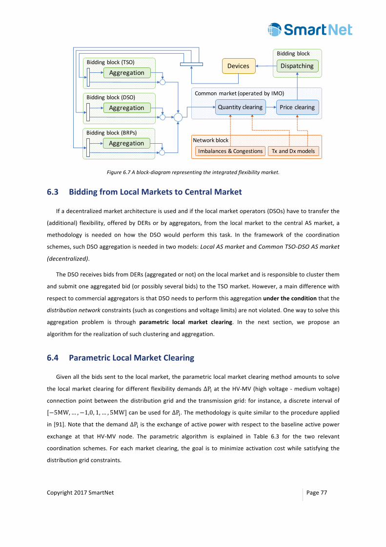
Copyright2017SmartNet Page77
Figure6.7Ablock-diagramrepresentingtheintegratedflexibilitymarket.
6.3 BiddingfromLocalMarketstoCentralMarket
Ifadecentralizedmarketarchitectureisusedandifthelocalmarketoperators(DSOs)havetotransferthe
(additional) flexibility,offeredbyDERsorbyaggregators, fromthe localmarket to thecentralASmarket,a
methodology is needed on how the DSO would perform this task. In the framework of the coordination
schemes,suchDSOaggregationisneededintwomodels:LocalASmarketandCommonTSO-DSOASmarket
(decentralized).
TheDSOreceivesbidsfromDERs(aggregatedornot)onthelocalmarketandisresponsibletoclusterthem
andsubmitoneaggregatedbid(orpossiblyseveralbids)totheTSOmarket.However,amaindifferencewith
respecttocommercialaggregatorsisthatDSOneedstoperformthisaggregationundertheconditionthatthe
distributionnetworkconstraints(suchascongestionsandvoltagelimits)arenotviolated.Onewaytosolvethis
aggregation problem is through parametric local market clearing. In the next section, we propose an
algorithmfortherealizationofsuchclusteringandaggregation.
6.4 ParametricLocalMarketClearing
Givenallthebidssenttothelocalmarket,theparametriclocalmarketclearingmethodamountstosolve
the localmarketclearing fordifferent flexibilitydemands∆PHat theHV-MV(highvoltage -mediumvoltage)
connectionpointbetweenthedistributiongridandthetransmissiongrid: for instance,adiscrete intervalof
[−5MW,… ,−1,0, 1, … , 5MW]canbeusedfor∆PH.Themethodologyisquitesimilartotheprocedureapplied
in[91].Notethatthedemand∆PH istheexchangeofactivepowerwithrespecttothebaselineactivepower
exchange at that HV-MV node. The parametric algorithm is explained in Table 6.3 for the two relevant
coordination schemes. For eachmarket clearing, the goal is tominimize activation costwhile satisfying the
distributiongridconstraints.
Biddingblock(TSO)Biddingblock
Commonmarket(operatedbyIMO)
Priceclearing
DispatchingDevicesAggregation
Networkblock
Imbalances&Congestions TxandDxmodels
QuantityclearingBiddingblock(DSO)
Aggregation
Biddingblock(BRPs)
Aggregation
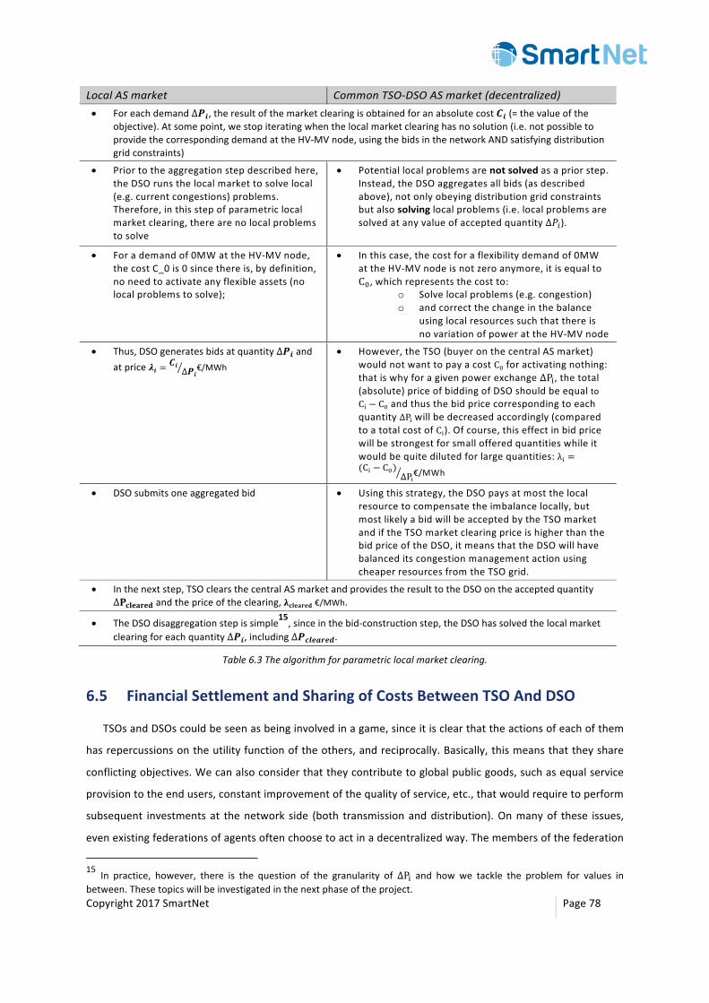
Copyright2017SmartNet Page78
LocalASmarket CommonTSO-DSOASmarket(decentralized)• Foreachdemand∆𝑷𝒊,theresultofthemarketclearingisobtainedforanabsolutecost𝑪𝒊(=thevalueofthe
objective).Atsomepoint,westopiteratingwhenthelocalmarketclearinghasnosolution(i.e.notpossibletoprovidethecorrespondingdemandattheHV-MVnode,usingthebidsinthenetworkANDsatisfyingdistributiongridconstraints)
• Priortotheaggregationstepdescribedhere,theDSOrunsthelocalmarkettosolvelocal(e.g.currentcongestions)problems.Therefore,inthisstepofparametriclocalmarketclearing,therearenolocalproblemstosolve
• Potentiallocalproblemsarenotsolvedasapriorstep.Instead,theDSOaggregatesallbids(asdescribedabove),notonlyobeyingdistributiongridconstraintsbutalsosolvinglocalproblems(i.e.localproblemsaresolvedatanyvalueofacceptedquantity∆𝑃)).
• Forademandof0MWattheHV-MVnode,thecostC_0is0sincethereis,bydefinition,noneedtoactivateanyflexibleassets(nolocalproblemstosolve);
• Inthiscase,thecostforaflexibilitydemandof0MWattheHV-MVnodeisnotzeroanymore,itisequaltoC3,whichrepresentsthecostto:
o Solvelocalproblems(e.g.congestion)o andcorrectthechangeinthebalance
usinglocalresourcessuchthatthereisnovariationofpowerattheHV-MVnode
• Thus,DSOgeneratesbidsatquantity∆𝑷𝒊andatprice𝝀𝒊 =
𝑪𝒊∆𝑷𝒊€/MWh
• However,theTSO(buyeronthecentralASmarket)wouldnotwanttopayacostC3 foractivatingnothing:thatiswhyforagivenpowerexchange∆PH,thetotal(absolute)priceofbiddingofDSOshouldbeequaltoCH − C3 andthusthebidpricecorrespondingtoeachquantity∆PHwillbedecreasedaccordingly(comparedtoatotalcostofCH).Ofcourse,thiseffectinbidpricewillbestrongestforsmallofferedquantitieswhileitwouldbequitedilutedforlargequantities:λH =(CH − C3)
∆PH€/MWh
• DSOsubmitsoneaggregatedbid • Usingthisstrategy,theDSOpaysatmostthelocalresourcetocompensatetheimbalancelocally,butmostlikelyabidwillbeacceptedbytheTSOmarketandiftheTSOmarketclearingpriceishigherthanthebidpriceoftheDSO,itmeansthattheDSOwillhavebalanceditscongestionmanagementactionusingcheaperresourcesfromtheTSOgrid.
• Inthenextstep,TSOclearsthecentralASmarketandprovidestheresulttotheDSOontheacceptedquantity∆𝐏𝐜𝐥𝐞𝐚𝐫𝐞𝐝andthepriceoftheclearing,𝛌𝐜𝐥𝐞𝐚𝐫𝐞𝐝€/MWh.
• TheDSOdisaggregationstepissimple15,sinceinthebid-constructionstep,theDSOhassolvedthelocalmarketclearingforeachquantity∆𝑷𝒊,including∆𝑷𝒄𝒍𝒆𝒂𝒓𝒆𝒅.
Table6.3Thealgorithmforparametriclocalmarketclearing.
6.5 FinancialSettlementandSharingofCostsBetweenTSOAndDSO
TSOsandDSOscouldbeseenasbeinginvolvedinagame,sinceitisclearthattheactionsofeachofthem
hasrepercussionsontheutilityfunctionoftheothers,andreciprocally.Basically,thismeansthattheyshare
conflictingobjectives.Wecanalsoconsiderthattheycontributetoglobalpublicgoods,suchasequalservice
provisiontotheendusers,constantimprovementofthequalityofservice,etc.,thatwouldrequiretoperform
subsequent investments at thenetwork side (both transmissionanddistribution).Onmanyof these issues,
evenexistingfederationsofagentsoftenchoosetoactinadecentralizedway.Themembersofthefederation
15 In practice, however, there is the question of the granularity of∆PH and how we tackle the problem for values inbetween.Thesetopicswillbeinvestigatedinthenextphaseoftheproject.

Copyright2017SmartNet Page79
can choose to provide the good in a centralized way. This implies that they will delegate the voluntary
provisiontoacentralized level,whichmaximizes their total surplus. If theychoosetoprovidethegood ina
decentralizedway,eachmembermaximizesitsownsurplusindependently.
Thereexistmanywaysofsharingthesocialwelfare(orthesumoftheactivationcosts)betweenDSOsand
theTSO.Themechanismsthatareproposed inthecooperativegametheory literaturerelyonbothfairness
andstabilitycriteria(Shapleyvalue,Banzhaf index,nucleolus,etc.).Thistopicwillbefurtherexplored inthe
nextphaseoftheproject.

Copyright2017SmartNet Page80
7 Conclusions
In this document, we provide the mathematical description of necessary modules which comprise the
IntegratedReservemarket,namelybidding,network,clearing,andpricing.Thesecomponentscanbearranged
andconnected invarioussetups, inorder toadapt themarket fora specific coordinationschemebetween
TSOandDSO.Thekeymessagesineachpartaresummarizedbelow.
7.1 Bidding
InChapter3wedefineacatalogueofmarketproducts(bids)andtheaccompanyingconstraintswhichare
allowedintheIntegratedReservemarket.Thebidsrepresentthedesiretoexchangeaquantityofpowerata
givenprice.Theaccompanyingconstraintsareusedtoimpressthosephysicallimitationsofflexibleresources
whichcannotbedescribedbythebiditself.Welistandformulatelogicalandtemporalconstraintswhichare
mostrelevanttoresourcesavailableatthemomentorinforeseeablefuture.
7.2 Network
Chapters4providethemodelsofpowernetwork,withanoptimization-orientedpointofview.Inaddition
to themathematicalmodeling, several topics such as the trade-off betweenmodel complexity and level of
detail, identificationandestimationofnetworkvariables (power flows,voltages,etc.)andcostofmodelling
errors are discussed. Since integer variables exist within the market clearing constraints, the approaches
proposed depend on convex approximations of the power flow physics, which allow to develop a mixed-
integerconvexmodelhavingsuperiortractability.
It is shown that in somecases, theSOCPBFMDistFlowsolution (globaloptimum) is actually superior to
those obtained by local non-convex solvers. Also, the simplified DistFlow formulation offers a high-quality
approximationintermsoffeasibilityandoptimality.
7.3 ClearingandPricing
The mathematical formulation of market clearing and pricing algorithms, which is the core of the
optimization problem, is described in Chapter 5. A first keymessage is that the objective of themarket is
highly affected by several pre-defined conventions, such as types of bids allowed (simple and complex
products),quantity/priceconvention(whetherbothpositiveandnegativequantitiesandpricesexist),network
model complexity (linearity and convexity), and the type of objective (cost minimization versus welfare
maximization).Furthermore,manyparametervaluescanaffectthebehaviorandalsotheperformanceofthe
clearingalgorithm.Someimportantones includethedurationoftimestep,thelengthofpredictionhorizon,
andthefrequencyofclearing.

Copyright2017SmartNet Page81
We show that it is possible to avoid unnecessary activation of resources, hence reducing the costs of
system operators, by adapting the prices of some bids. In this method, the objective will be kept as
maximizationofsocialwelfare,whichisrecommendedbyENTSOE.
Ingeneral, thepricingprocess,which isdefinedasadualproblemofthequantityclearing,canhavethe
same complexities as theprimal problem.However, there are severalmethods to avoid these complexities
andfindthelocationalmarginalpricesinamorestraight-forwardandintuitiveway.Insightintothistopicare
providedinChapter4andamorethoroughdiscussionwillbeprovidedinthefinalversionofthisdocument,
i.e.deliverableD2.2.
7.4 CoordinationSchemes
Chapter6summarizesthestructureofmarketundereachTSO-DSOcoordinationscheme.Inthisschematic
presentation, it is shown how different market modules can be used to create a setup suitable for each
coordinationscheme.Thesedescriptionswillbeadaptedasthemarket-implementationstageoftheSmartNet
projecthasbegun,throughacontinuousfeedbackloop.FinalizeddetailswillbeavailableindeliverableD2.2.
Copyright2017SmartNet Page82
8 References
[1] H.Gerard,E.Rivero,andD.Six, “BasicschemesforTSO-DSOcoordinationandancillaryservicesprovision,”SmartNetProject,D1.3,2016.
[2] J.Merinoetal.,“AncillaryserviceprovisionbyRESandDSMconnectedatdistributionlevelinthefuturepowersystem,”SmartNetProject,D1.1,2016.
[3] M. Kohansal and H. Mohsenian-Rad, “A closer look at demand bids in California ISO energymarket,”IEEETrans.PowerSyst.,vol.31,no.4,pp.3330–3331,2016.
[4] “SmartNet Project - Consultations,” 2016. [Online]. Available: http://smartnet-project.eu/consultations/.
[5] M.Dzamarija,“Aggregationmodels,”SmartNetProject,D2.3,2017.
[6] J.Carpentier,“Contributional’etudedudispatchingeconomique,”Bull.laSoc.Fr.desElectr.,vol.3,no.1,pp.431–447,1962.
[7] H.W.DommelandW.F.Tinney,“Optimalpowerflowsolutions,”IEEETrans.powerAppar.Syst.,no.10,pp.1866–1876,1968.
[8] O. Alsac and B. Stott, “Optimal load flowwith steady-state security,” IEEE Trans. power Appar.Syst.,no.3,pp.745–751,1974.
[9] B. Stott andO. Alsaç, “Optimal power flow--basic requirements for real-life problems and theirsolutions,”inSEPOPEXIISymposium,RiodeJaneiro,Brazil,2012.
[10] F. Capitanescu et al., “State-of-the-art, challenges, and future trends in security constrainedoptimalpowerflow,”Electr.PowerSyst.Res.,vol.81,no.8,pp.1731–1741,2011.
[11] M. E. Baran and F. F. Wu, “Optimal capacitor placement on radial distribution systems,” IEEETrans.powerDeliv.,vol.4,no.1,pp.725–734,1989.
[12] L.VandenbergheandS.Boyd, “Semidefiniteprogramming,”SIAMRev., vol. 38, no. 1, pp. 49–95,1996.
[13] N. Z. Shor, “Quadratic optimization problems,”Sov. J. Comput. Syst. Sci., vol. 25, no. 6, pp. 1–11,1987.
[14] J.B.Lasserre,“Globaloptimizationwithpolynomialsandtheproblemofmoments,”SIAMJ.Optim.,vol.11,no.3,pp.796–817,2001.
[15] S. Kim,M.Kojima, andM. Yamashita, “Secondorder coneprogramming relaxation of a positivesemidefiniteconstraint,”Optim.MethodsSoftw.,vol.18,no.5,pp.535–541,2003.
[16] A.Ashouri,“SimultaneousDesignandControlofEnergySystems,”ETHZurich,2014.
[17] M.Lubin,E.Yamangil,R.Bent,andJ.P.Vielma,“Extendedformulations inmixed-integerconvexprogramming,” in International Conference on Integer Programming and CombinatorialOptimization,2016,pp.102–113.
[18] J.A.Taylor,Convexoptimizationofpowersystems.CambridgeUniversityPress,2015.
[19] A. Ben-Tal andA.Nemirovski, “Onpolyhedral approximations of the second-order cone,”Math.Oper.Res.,vol.26,no.2,pp.193–205,2001.
[20] R.A. Jabr, “Radialdistribution load flowusingconicprogramming,” IEEETrans.powerSyst.,vol.
Copyright2017SmartNet Page83
21,no.3,pp.1458–1459,2006.
[21] S. H. Low, “Convex relaxation of optimal power flow, part II: Exactness,” arXiv Prepr.arXiv1405.0814,2014.
[22] D.K.MolzahnandI.A.Hiskens,“MixedSDP/SOCPmomentrelaxationsoftheoptimalpowerflowproblem,”inPowerTech,2015IEEEEindhoven,2015,pp.1–6.
[23] B. Ghaddar, J. Marecek, and M. Mevissen, “Optimal power flow as a polynomial optimizationproblem,”IEEETrans.PowerSyst.,vol.31,no.1,pp.539–546,2016.
[24] C.Josz,J.Maeght,P.Panciatici,andJ.C.Gilbert,“Applicationofthemoment-SOSapproachtoglobaloptimizationoftheOPFproblem,”IEEETrans.PowerSyst.,vol.30,no.1,pp.463–470,2015.
[25] R.A.Jabr,“Aconicquadraticformatfortheloadflowequationsofmeshednetworks,”IEEETrans.PowerSyst.,vol.22,no.4,pp.2285–2286,2007.
[26] R.A.Jabr,“Optimalpowerflowusinganextendedconicquadraticformulation,”IEEETrans.powerSyst.,vol.23,no.3,pp.1000–1008,2008.
[27] R. A. Jabr, R. Singh, and B. C. Pal, “Minimum loss network reconfiguration usingmixed-integerconvexprogramming,”IEEETrans.PowerSyst.,vol.27,no.2,pp.1106–1115,2012.
[28] H.L.HijaziandS.Thiébaux,“Optimalacdistributionsystemsreconfiguration,” inPowerSystemsComputationConference(PSCC),2014,2014,pp.1–7.
[29] C.Coffrin,D.Gordon,andP.Scott,“Nesta,theNICTAenergysystemtestcasearchive,”arXivPrepr.arXiv1411.0359,2014.
[30] C.Coffrin,H.Hijazi,andP.VanHentenryck,“StrengtheningtheSDPRelaxationofACPowerFlowswith Convex Envelopes, Bound Tightening, and Lifted Nonlinear Cuts,” arXiv Prepr.arXiv1512.04644,2015.
[31] C.Coffrin,H.L.Hijazi,andP.VanHentenryck,“Theqcrelaxation:Theoreticalandcomputationalresultsonoptimalpowerflow,”arXivPrepr.arXiv1502.07847,2015.
[32] H. Hijazi, C. Coffrin, and P. Van Hentenryck, “Convex quadratic relaxations for mixed-integernonlinearprogramsinpowersystems,”Math.Program.Comput.,pp.1–47,2014.
[33] C.Coffrin,H.L.Hijazi,andP.VanHentenryck,“NetworkFlowandCopperPlateRelaxationsforACTransmissionSystems,”arXivPrepr.arXiv1506.05202,2015.
[34] R. Berg, E. S. Hawkins, andW.W. Pleines, “Mechanized calculation of unbalanced load flow onradialdistributioncircuits,”IEEETrans.PowerAppar.Syst.,no.4,pp.415–421,1967.
[35] T.-H. Chen,M.-S. Chen, K.-J. Hwang, P. Kotas, and E. A. Chebli, “Distribution system power flowanalysis-arigidapproach,”IEEETrans.PowerDeliv.,vol.6,no.3,pp.1146–1152,1991.
[36] C.S.ChengandD.Shirmohammadi,“Athree-phasepowerflowmethodforreal-timedistributionsystemanalysis,”IEEETrans.PowerSyst.,vol.10,no.2,pp.671–679,1995.
[37] M.E.BaranandF.F.Wu,“Networkreconfigurationindistributionsystemsforlossreductionandloadbalancing,”IEEETrans.PowerDeliv.,vol.4,no.2,pp.1401–1407,1989.
[38] L. Gan and S. H. Low, “Convex relaxations and linear approximation for optimal power flow inmultiphaseradialnetworks,”inPowerSystemsComputationConference(PSCC),2014,2014,pp.1–9.
[39] D. K.Molzahn, J. T. Holzer, B. C. Lesieutre, and C. L. DeMarco, “Implementation of a large-scaleoptimalpowerflowsolverbasedonsemidefiniteprogramming,”IEEETrans.PowerSyst.,vol.28,no.4,pp.3987–3998,2013.
Copyright2017SmartNet Page84
[40] X. Bai, H. Wei, K. Fujisawa, and Y. Wang, “Semidefinite programming for optimal power flowproblems,”Int.J.Electr.PowerEnergySyst.,vol.30,no.6,pp.383–392,2008.
[41] R.Madani, S. Sojoudi, and J. Lavaei, “Convex relaxation for optimal power flow problem:Meshnetworks,”IEEETrans.PowerSyst.,vol.30,no.1,pp.199–211,2015.
[42] J.Lavaei,S.Member,andS.H.Low,“ZeroDualityGapinOptimalPowerFlowProblem,”vol.27,no.1,pp.92–107,2012.
[43] L.GanandS.H. Low, “Chordal relaxationofOPF formultiphase radialnetworks,” in2014 IEEEInternationalSymposiumonCircuitsandSystems(ISCAS),2014,pp.1812–1815.
[44] S.Bose,S.H.Low,T.Teeraratkul,andB.Hassibi,“Equivalentrelaxationsofoptimalpowerflow,”IEEETrans.Automat.Contr.,vol.60,no.3,pp.729–742,2015.
[45] S. Mhanna, G. Verbic, and A. Chapman, “Tight LP Approximations for the Optimal Power FlowProblem,”arXivPrepr.arXiv1603.00773,2016.
[46] C. Coffrin and P. Van Hentenryck, “A linear-programming approximation of AC power flows,”INFORMSJ.Comput.,vol.26,no.4,pp.718–734,2014.
[47] Federal Energy Regulatory Commission, “FERC - optimal power flow and formulation papers,”2013. [Online]. Available: http://www.ferc.gov/industries/electric/indus-act/market-planning/opf-papers.asp.
[48] A.CastilloandR.P.O’Neill, “SurveyofapproachestosolvingtheACOPF(OPFPaper4),”USFed.EnergyRegul.Comm.Tech.Rep,2013.
[49] F. Capitanescu, “Critical review of recent advances and further developments needed in ACoptimalpowerflow,”Electr.PowerSyst.Res.,vol.136,pp.57–68,2016.
[50] S.H.Low,“Convexrelaxationofoptimalpowerflow,partI:Formulationsandequivalence,”arXivPrepr.arXiv1405.0766,2014.
[51] S. H. Low, “Convex relaxation of optimal power flow: a tutorial,” in2013 IREP SymposiumBulkPowerSystemDynamicsandControl-IXOptimization,SecurityandControlof theEmergingPowerGrid,2013.
[52] L. Gan, “Distributed load control in multiphase radial networks,” California Institute ofTechnology,2015.
[53] L. Gan, N. Li, U. Topcu, and S. H. Low, “Exact convex relaxation of optimal power flow in treenetworks,”arXivPrepr.arXiv1208.4076,2012.
[54] L.Gan,N.Li,U.Topcu,andS.Low,“Ontheexactnessofconvexrelaxationforoptimalpowerflowin tree networks,” in 2012 IEEE 51st IEEE Conference on Decision and Control (CDC), 2012, pp.465–471.
[55] L.Gan,S.H.Low,andC.EAS,“ConvexificationofACoptimalpowerflow,”inProc.ofthe18thPowerSystemsComputationConference(PSCC),Wroclaw,Poland,2014.
[56] R.Madani,M.Ashraphijuo,andJ.Lavaei,“Sdpsolverofoptimalpowerflowusersmanual,”2014.
[57] S.Sojoudiand J.Lavaei, “Physicsofpowernetworksmakeshardoptimizationproblemseasy tosolve,”in2012IEEEPowerandEnergySocietyGeneralMeeting,2012,pp.1–8.
[58] A. Castillo and others, “Essays on the ACOPF Problem: Formulations, Approximations, andApplicationsintheElectricityMarkets,”JohnsHopkinsUniversity,2016.
[59] M. Farivar, “Optimization and Control of Power Flow in Distribution Networks,” CaliforniaInstituteofTechnology,2016.
Copyright2017SmartNet Page85
[60] D.Mayer,“HamiltonsPrincipleandElectricCircuitsTudory,”Adv.Electr.Electron.Eng.,vol.5,no.1–2,p.185,2006.
[61] H. Andrei, P. C. Andrei, G. Oprea, andB. Botea, “Basic equations of linear electric andmagneticcircuitsinquasi-stationarystatebasedonprincipleofminimumabsorbedpowerandenergy,”inFundamentalsofElectricalEngineering(ISFEE),2014InternationalSymposiumon,2014,pp.1–6.
[62] H.AndreiandF.Spinei,“Anextensionoftheminimumenergyprinciple instationaryregimeforelectricandmagneticcircuits,”Rev.Roum.desSci.Tech.Ser.Electrotech.Energ., vol.52,no.4,p.419,2007.
[63] J.E.Prussing,“Theprincipalminortestforsemidefinitematrices,”J.Guid.Control.Dyn.,vol.9,no.1,pp.121–122,1986.
[64] M. Fazel, H. Hindi, and S. P. Boyd, “Log-det heuristic for matrix rank minimization withapplications to Hankel and Euclidean distancematrices,” inAmerican Control Conference, 2003.Proceedingsofthe2003,2003,vol.3,pp.2156–2162.
[65] K. Mohan and M. Fazel, “Reweighted nuclear norm minimization with application to systemidentification,”inProceedingsofthe2010AmericanControlConference,2010,pp.2953–2959.
[66] R. Louca, P. Seiler, and E. Bitar, “A rank minimization algorithm to enhance semidefiniterelaxations of optimal power flow,” in Communication, Control, and Computing (Allerton), 201351stAnnualAllertonConferenceon,2013,pp.1010–1020.
[67] R. Madani, M. Ashraphijuo, and J. Lavaei, “Promises of conic relaxation for contingency-constrainedoptimalpowerflowproblem,”IEEETrans.PowerSyst.,vol.31,no.2,pp.1297–1307,2016.
[68] D. Shi, “Powersystemnetwork reduction forengineeringandeconomicanalysis,”ArizonaStateUniversity,2012.
[69] Dj. M. Dobrijevic and D. P. Popovic, “An unified external network equivalent in steady-statesecurityassessment,”FactaUniv.Electron.Energ.,vol.23,no.2,pp.179–189,2010.
[70] F. Milano and K. Srivastava, “Dynamic REI equivalents for short circuit and transient stabilityanalyses,”Electr.PowerSyst.Res.,vol.79,no.6,pp.878–887,2009.
[71] K.VanDenBergh,E.Delarue,andW.D’haeseleer, “DCpower flowinunitcommitmentmodels,”no.May,2014.
[72] D. Shi and D. J. Tylavsky, “An improved bus aggregation technique for generating networkequivalents,”in2012IEEEPowerandEnergySocietyGeneralMeeting,2012,pp.1–8.
[73] T. Pang-Ning, M. Steinbach, V. Kumar, and others, “Introduction to data mining,” in Library ofcongress,2006,vol.74.
[74] N. Muller and V. K. Quintana, “A sparse eigenvalue-based approach for partitioning powernetworks,”IEEETrans.powerSyst.,vol.7,no.2,pp.520–527,1992.
[75] M. Gavrilas, O. Ivanov, and G. Gavrilas, “REI equivalent design for electric power systemswithgeneticalgorithms,”WSEASTrans.CircuitsSyst.,vol.7,no.10,pp.911–921,2008.
[76] Q.Zhai,X.Guan,J.Cheng,andH.Wu,“FastidentificationofinactivesecurityconstraintsinSCUCproblems,”IEEETrans.PowerSyst.,vol.25,no.4,pp.1946–1954,2010.
[77] R. Fernández-Blanco, J. M. Arroyo, N. Alguacil, and X. Guan, “Incorporating Price-ResponsiveDemand in Energy Scheduling Based on Consumer Payment Minimization,” IEEE Trans. SmartGrid,vol.7,no.2,pp.817–826,2016.
[78] A. J. Ardakani and F. Bouffard, “Identification of umbrella constraints in DC-based security-
Copyright2017SmartNet Page86
constrainedoptimalpowerflow,”IEEETrans.PowerSyst.,vol.28,no.4,pp.3924–3934,2013.
[79] A. J. Ardakani and F. Bouffard, “Acceleration of umbrella constraint discovery in generationschedulingproblems,”IEEETrans.PowerSyst.,vol.30,no.4,pp.2100–2109,2015.
[80] A. Zani and G. Migliavacca, “Pan-European balancing market: Benefits for the Italian powersystem,” in AEIT Annual Conference-From Research to Industry: The Need for a More EffectiveTechnologyTransfer(AEIT),2014,2014,pp.1–6.
[81] S. F. Tierney, T. Schatzki, and R. Mukerji, “Uniform-pricing versus pay-as-bid in wholesaleelectricitymarkets:doesitmakeadifference?,”NewYorkISO,2008.
[82] F.C.Schweppe,M.C.Caramanis,R.D.Tabors,andR.E.Bohn,Spotpricingofelectricity.SpringerScience&BusinessMedia,2013.
[83] R.E.Bohn,M.C.Caramanis,andF.C.Schweppe,“Optimalpricinginelectricalnetworksoverspaceandtime,”RandJ.Econ.,pp.360–376,1984.
[84] S.S.Oren,“MarketDesignandGaminginCompetitiveElectricityMarkets.”
[85] A.EhrenmannandY.Smeers,“InefficienciesinEuropeancongestionmanagementproposals,”Util.policy,vol.13,no.2,pp.135–152,2005.
[86] E. Bjorndal,M.H. Bjorndal,H. Cai, andE. Panos, “Hybrid Pricing in a CoupledEuropeanPowerMarketwithMoreWindPower,”NHHDept.Bus.Manag.Sci.Discuss.Pap.,no.2015/28,2015.
[87] M.C.Ferris,S.P.Dirkse,andA.Meeraus, “Mathematicalprogramswithequilibriumconstraints:Automaticreformulationandsolutionviaconstrainedoptimization,”2002.
[88] S.Oren,“Whenisapay-asbidpreferabletouniformpriceinelectricitymarkets,”inPowerSystemsConferenceandExposition,2004,vol.3,pp.1618–1620.
[89] M.MarracciandD.Poli,“AnalysisofthePossibleImpactofComplexBidsintheItalianElectricitySpot Market,” in International Conference on Energy, Environment, Devices, Systems,Communications,Computers,2011.
[90] G. Leclercq, M. Z. Degefa, G. Vigano, and J. Le Baut, “Characterization of flexible resources anddistributionnetworks,”SmartNetProject,D1.2,2017.
[91] M. Mashhour, M. A. Golkar, and S. M. Moghaddas-Tafreshi, “Extending market activities for adistributioncompanyinhourly-aheadenergyandreservemarkets--PartI:Problemformulation,”EnergyConvers.Manag.,vol.52,no.1,pp.477–486,2011.
[92] J. Lofberg, “YALMIP: A toolbox for modeling and optimization in MATLAB,” in Computer AidedControlSystemsDesign,2004IEEEInternationalSymposiumon,2004,pp.284–289.
[93] B. De Tandt, “EN50160 -- Voltage characteristics of electricity supplied by public distributionsystems,”Eur.Comm.Electrotech.Stand.,1999.
[94] G.Andersson,“Modellingandanalysisofelectricpowersystems,”EEH-PowerSyst.Lab.SwissFed.Inst.Technol.(ETH),Zürich,Switz.,2004.
[95] M. Fazel,H.Hindi, and S. P. Boyd, “A rankminimization heuristicwith application tominimumorder system approximation,” in American Control Conference, 2001. Proceedings of the 2001,2001,vol.6,pp.4734–4739.
[96] ENTSO-E,“PhaseShiftTransformersModelling.”2014.
[97] D.Povhandothers, “Load flowcontrol inhighvoltagepowersystemsusingFACTScontrollers,”CigreTF,pp.1–38,1996.

Copyright2017SmartNet Page87
[98] F. Li and R. Bo, “DCOPF-based LMP simulation: algorithm, comparison with ACOPF, andsensitivity,”IEEETrans.PowerSyst.,vol.22,no.4,pp.1475–1485,2007.
[99] R.D.Zimmerman,C.E.Murillo-Sánchez,andR.J.Thomas,“MATPOWER:Steady-stateoperations,planning,andanalysistoolsforpowersystemsresearchandeducation,”IEEETrans.powerSyst.,vol.26,no.1,pp.12–19,2011.
[100] K.Purchala,L.Meeus,D.VanDommelen,andR.Belmans,“UsefulnessofDCpowerflowforactivepower flow analysis,” in IEEE Power Engineering Society GeneralMeeting, 2005, 2005, pp. 454–459.
[101] R. A. Jabr, “Polyhedral formulations and loop elimination constraints for distribution networkexpansionplanning,”IEEETrans.PowerSyst.,vol.28,no.2,pp.1888–1897,2013.
[102] F.Geth,C.delMarmol,D.Laudy,andC.Merckx,“Mixed-integersecond-orderconeunitmodelsforcombined active-reactive power optimization,” in Energy Conference (ENERGYCON), 2016 IEEEInternational,2016,pp.1–6.
[103] K. Heussen, S. Koch, A. Ulbig, and G. Andersson, “Unified system-levelmodeling of intermittentrenewableenergysourcesandenergystorageforpowersystemoperation,”IEEESyst.J.,vol.6,no.1,pp.140–151,2012.
[104] M.Farivar,C.R.Clarke,S.H.Low,andK.M.Chandy,“Invertervarcontrolfordistributionsystemswith renewables,” in Smart Grid Communications (SmartGridComm), 2011 IEEE InternationalConferenceon,2011,pp.457–462.
[105] F.Piloetal.,“ATLANTIDE—DigitalarchiveoftheItalianelectricdistributionreferencenetworks,”inIntegrationofRenewablesintotheDistributionGrid,CIRED2012Workshop,2012,pp.1–4.
[106] S. Diamond and S. Boyd, “CVXPY: A Python-embedded modeling language for convexoptimization,”J.Mach.Learn.Res.,vol.17,no.83,pp.1–5,2016.
[107] A. Domahidi, E. Chu, and S. Boyd, “ECOS: An SOCP solver for embedded systems,” in ControlConference(ECC),2013European,2013,pp.3071–3076.
[108] R.Lincoln,“PYPOWER5.0.1.”2015.
[109] A.Papavasiliou,“OptimizationModelsinElectricityMarkets.”
[110] W.W.Hogan,“Contractnetworksforelectricpowertransmission,”J.Regul.Econ.,vol.4,no.3,pp.211–242,1992.
[111] P. R. Gribik,W.W.Hogan, and S. L. Pope, “Market-clearing electricity prices and energy uplift.”December,2007.
[112] R.P.O’Neill,P.M.Sotkiewicz,B.F.Hobbs,M.H.Rothkopf, andW.R.Stewart, “Efficientmarket-clearing prices inmarketswith nonconvexities,”Eur. J. Oper. Res., vol. 164, no. 1, pp. 269–285,2005.
[113] M. Madani and M. Van Vyve, “Computationally efficient MIP formulation and algorithms forEuropeanday-aheadelectricitymarket auctions,”Eur. J.Oper.Res., vol. 242,no.2,pp.580–593,2015.
[114] IndustRE, “Deliverable 2.2: Regulatory and Market Framework Analysis.” [Online]. Available:www.industre.eu/downloads/download/regulatory-and-market-framework-analysis.

Copyright2017SmartNet Page88
9 Appendices
9.1 FormulationofBidsandConstraints
9.1.1 Nomenclature:ConstantsandVariables
In this section, constants and variableswhich are used to define the constraints and the objectives are
listed.
Constants(Scalars,SetsandMappings)
1. 𝛿𝑡:timesteporperiodatwhichtheenergymarketclearingisperformed.
2. 𝑇:numberoftimestepsconsideredinonerollingwindowoptimization.
3. 𝑁: the set of all nodes in the network (graph). For the considered tree-shaped distribution sub-
networks,𝑁denotesthesetofnodesofthetree-shapednetwork,exceptfortherootnode.
4. 𝛾l:timediscountfactorthat, intheobjectivefunction,weighsnear-futuretimeslotobjectiveterms
higherthanfar-futuretime slots.
5. 𝐴*:thesetofactors(aggregatorsoragents)atnode𝑛 ∈ 𝑁.
6. ∀𝑛 ∈ 𝑁, ∀𝑎 ∈ 𝐴*:
(a) 𝐵*+:setofbids.
(b) 𝐼*+:setofpairsofbidswithan‘implication’constraint.
(c) 𝑋*+:setofsetsofbidswith‘exclusivechoice’constraints.
7. ∀𝑛 ∈ 𝑁, ∀𝑎 ∈ 𝐴*, ∀𝑏 ∈ 𝐵*+:
(a) 𝑃𝐹*+´:powerfactor.
(b) 𝑥*+´: the minimal acceptance fraction for the variable 𝑥*+´. It holds for all primitive bids it
generates.
(c) 𝑎*+´,�4:theassumedcurrentstateofactivationoftheofferedbid.
(d) 𝛼*+´:maximalnumberofactivations(start-ups)intheoptimizationwindow.
(e) 𝛿*+´µ :minimalduration(timesteps)oftimeinwhichtheunitmustbeactivated.
(f) 𝛿*+´µ
:maximalduration(timesteps)oftimeinwhichtheunitcanbeactivated.

Copyright2017SmartNet Page89
(g) 𝛿*+´¶ :minimalduration(timesteps)oftime inwhichtheunitmustbedeactivated.Theparameter
𝛿*+´¶ has0asitsdefaultvalue.
(h) 𝛼*+´,·:Booleansindicatingthestartofactivationpriortocurrenttimestep.Thesemustbedefinedif
constraint (e) or (f) exists. For constraint (f), 𝜏 ∈ −𝛿*+´µ
+ 1, … , −2, −1 , and for constraint (e), ∀𝜏 ∈
−𝛿*+´µ + 1, … , −2, −1 .
(i) 𝜔*+´,·:Booleansindicatingstopofactivation(i.e.deactivation)priortocurrenttimestep.Thesemust
beavailableifconstraint(g)exists,inwhichcase𝜏 ∈ −𝛿*+´¶ + 1, … , −2, −1 .
(j) 𝛥𝑞*+´:maximaldecreaseofenergyquantityfromanytimesteptothenextone.
(k) 𝛥𝑞*+´:maximalincreaseofenergyquantityfromanytimesteptothenextone.
(l) 𝑇*+´:setof(consecutive)timestepsinaQtbid.
8. ∀𝑛 ∈ 𝑁, ∀𝑎 ∈ 𝐴*, ∀𝑏 ∈ 𝐵*+, ∀𝑡 ∈ 𝑇*+´:
(a) 𝑞*+´l:maximalavailablequantityofactivepowerforaprimitivebid(step/trapezoidal).
(b) 𝑝*+´l:biddingpriceatchosenquantity(correspondingtothemarginalcostsofthebidder).
(c) 𝑚*+´l: ℝ → ℝ:mappingofpowerquantity𝑞tomarginalcost(price)𝑝.Itimpliesthat𝑝 = 𝑚*+´l(𝑞)
(note that reactivepowerhasnodirectlyspecifiablemarginalcosthere.Abidder takes this indirectly into
accountviathepowerfactor𝑃𝐹*+´though.)
(d) 𝛱 = 𝛱*+´l:setofprimitivebids,resultingfromdecompositionontheQ-axis
(e) 𝛱k)À|l:subsetof𝛱,includingcommonbidswiththerightsignof𝑞(usefulforeliminationofsystem
imbalance).
(f) 𝛱ÁkÂ*À:subsetof𝛱, includingcommonbidswiththewrongsignof𝑞 (notusefulforeliminationof
systemimbalance).
Variables
Variablescanberealorbinary(orinteger,tobemoregeneral).Binaryvariablestakevaluesin 0,1 .
1. ∀𝑛 ∈ 𝑁, ∀𝑎 ∈ 𝐴*, ∀𝑏 ∈ 𝐵*+:
(a) 𝑎𝑎*+´ binary whichequals1 if thebid isactivatedforanytimestepwithinthehorizon.Thenwe
callthebid‘accepted’.
2. ∀𝑛 ∈ 𝑁, ∀𝑎 ∈ 𝐴*, ∀𝑏 ∈ 𝐵*+, ∀𝑡 ∈ 𝑇*+´:
(a) 𝑎*+´l(binary)whichequals1ifthebidisactivatedforthetimestept.
Copyright2017SmartNet Page90
(b) 𝛼*+´l(binary)whichequals1 for time stepatwhich thebidgoes fromnon-activated toactivated
(activationbegins).
(c) 𝜔*+´l(binary)whichequals1 for timestepatwhich thebidgoes fromactivated tonon-activated
(activationends).
3. ∀𝑛 ∈ 𝑁, ∀𝑎 ∈ 𝐴*, ∀𝑏 ∈ 𝐵*+, ∀𝑡 ∈ 𝑇*+´, ∀𝛽 ∈ 𝛱*+´l:
(a) 𝑥*+´l�(real): 0 ≤ 𝑥*+´l� ≤ 1:fractionofquantity𝑞*+´l�ofprimitivebid𝛽thatisactivated.
9.1.2 StructureofDataforDefinitionofBids
9.1.2.1 DefinitionofUNIT-bids
PracticallyUNIT-bidsincolumns1,2and3canrespectivelybespecifiedas:
1. (BID_ISSUER_ID,BID_ID,NETWORK_NODE_ID,UNIT_BID,STEP,NON_CURTAILABLE,POWER_FACTOR,Q0,P0),
2. (BID_ISSUER_ID,BID_ID,NETWORK_NODE_ID,UNIT_BID,STEP,CURTAILABLE,POWER_FACTOR,Q0,P0,Q1),
3. (BID_ISSUER_ID,BID_ID,NETWORK_NODE_ID,UNIT_BID,PWL,CURTAILABLE,POWER_FACTOR,Q0,P0,Q1,P1)
Someclarificationsontheindividualfieldsareprovidedhere:
1. ThementionedfieldBID_ISSUER_IDistheuniqueIDofeachmarketparticipant
2. The mentioned field BID_ID represents an identifier that uniquely identifies the bid amongst the
(current) bids of that particular bid issuer. Bid issuers are responsible for the uniqueness of BID_ID. If an
answertothisbidissentbacktothebidissuer,itwillcontainthisBID_IDsothatthebidissuerknowswhatbid
the answer is a response to. Note that the couple (BID_ISSUER_ID, BID_ID) uniquely identifies a bid in the
marketbutBID_IDalonedoesnot.
3. TheargumentUNIT_BIDdefinesthetypeofthebidregardingitsdimension,meaningthatitisnota
Q-bidnoraQt-bid.
4. Theidentifiers{STEP,CURTAILABLE},{STEP,NON_CURTAILABLE},and{PWL,CURTAILABLE}arethere
todistinguishamongthetypesofbidsregardingthequantity.Acurtailablestepbidcanonlyprovideafixed
quantity(orvolume)ifaccepted.Acurtailablestepbidmaybeacceptedatanyquantitybetweenzeroanda
maximumquantity(foraUNIT-bid).Apiece-wiselinearcurtailablebidissimilartoacurtailablestepbid,with
thedifferencethatitspricechangeslinearlywithchangingquantity.
5. ThementionedfieldNETWORK_NODE_IDcontainsavaluethatuniquelyidentifiesanodewithinthe
electricitynetworkmodelledinthemarketclearing.
6. The mentioned POWER_FACTOR gives the ratio of reactive power to the active power and is
supposedtobeconstantpertimestep.
Copyright2017SmartNet Page91
7. ThementionedfieldsQiandPicontainnumericalvaluesexpressedinenergyunitandcurrencyunit.
Forsimplicity,itisassumedthattheyarefixed(forallbids)toMWandEUR/MW,respectively.
9.1.2.2 DefinitionofQ-bids
Q-bidswithseveralpairsof 𝑞, 𝑝 incolumns1,2and3ofFigure3.2canrespectivelybespecifiedas:
1. (BID_ISSUER_ID,BID_ID,NETWORK_NODE_ID,UNIT_BID,STEP,NON_CURTAILABLE,POWER_FACTOR,Q0,P0,
Q1,P1,...,Qn-1,Pn-1),
2. (BID_ISSUER_ID,BID_ID,NETWORK_NODE_ID,UNIT_BID,STEP,CURTAILABLE,POWER_FACTOR,Q0,P0,Q1,P1,
...,Qn-1,Pn-1),
3. (BID_ISSUER_ID,BID_ID,NETWORK_NODE_ID,UNIT_BID,PWL,CURTAILABLE,POWER_FACTOR,Q0,P0,Q1,P1,
...,Qn-1,Pn-1)
Becausewewanttoallowanaggregator topotentiallyofferbothpower injection (positiveQ)aswellas
power offtake (negative Q) from the network, we allow a general Q-bid to specify prices for a range of
quantitiesthatcangenerallygofromanegativetoapositivevalue.
It follows from the principle of themerit-order acceptance of bids, thatwe require, that the Pi on the
positiveenergysideareincreasingwithincreasinglypositiveQ,andthePionthenegativesideareincreasing
withincreasinglynegativeQ.(TheactualSTEPcurvecanstillhaveflatparts).Notethatthereisnorestriction
onpositiveornegativepricesandnoapriorirestrictiononconvexityoftheassociatedcurve.
9.1.2.3 DefinitionofQt-bids
Qt-bidsincolumns1,2and3ofFigure3.2canbespecifiedas:
(BID_ISSUER_ID,BID_ID,NETWORK_NODE_ID,UNIT_BID,STEP,NON_CURTAILABLE,
t=0,Q0,P0,Q1,P1,...,Qn-1,Pn-1,POWER_FACTOR,
t=1,Q0,P0,Q1,P1,...,Qn-1,Pn-1,POWER_FACTOR,
…
t=11,Q0,P0,Q1,P1,...,Qn-1,Pn-1,POWER_FACTOR)
andsimilarly,forthe(BID_ISSUER_ID,BID_ID,NETWORK_NODE_ID,UNIT_BID,STEP,CURTAILABLE,…)and
(BID_ISSUER_ID,BID_ID,NETWORK_NODE_ID,UNIT_BID,PWL,CURTAILABLE,…)forms.Here,t=0referstothe
firstdecision timestepand t=11 to the twelfthone (ifweassume5-minute time stepwitha1hour rolling
optimizationhorizon).Notethatthedecisiontimestepsizewillbefixedinthemarketsystemandknownto
marketparticipants.
9.1.3 DefinitionofAcceptance

Copyright2017SmartNet Page92
9.1.3.1 AcceptanceofaQ-bid
WecallaQ-bid‘accepted’,ifanyofthesequenceofitsprimitivebidsitiscomposedofisactivatedfor
a fraction 𝑥 larger than 0. The Boolean variable 𝑎*+´l indicates whether the bid is activated or not.
Whetherthisisthecaseornotcanbederivedfromtheacceptanceofitscomposingprimitivebidsbythe
constraints
𝑎*+´l ⋅ 𝑥*+´ ≤ 𝑥*+´l�
�∈�ÉÊËÌ
≤ 𝑎*+´l ⋅ 𝛱*+´l (26)
where 𝛱*+´l isthenumberofelementsintheset𝛱*+´land𝑥*+´istheminimumacceptancefraction
atwhichacceptanceisconsideredrelevant,forexample0.01. If intheleft-handsideof(26),𝑎*+´l = 1,
the summation in themiddle part is bigger than 0, so at least one𝑥*+´l� is forced to be non-zero. If
𝑎*+´l = 0,theright-handsideforcesthesummationinthemiddleparttobe0,soall𝑥*+´l�areforcedto
bezero.
Theconstraints
∀𝛽 ∈ 𝛱*+´l,𝑥*+´l� ≤ 𝑎*+´l (27)
can be added on top, but are not strictly necessary. If they turn out to be speeding up the
optimization,theycanbeadded.
9.1.3.2 AcceptanceofaQt-bid
WecallaQt-bid‘accepted’iftheQ-bidforany(atleastone)ofitstimestepshasbeenaccepted.This
isimposedbythefollowingconstraints:
𝑎𝑎*+´ ⋅ 𝑥*+´ ≤ 𝑎*+´ll∈�ÉÊË ≤ 𝑎𝑎*+´ ⋅ 𝑇*+´ . (28)
When𝑎𝑎*+´ = 0, theright-handsideforces𝑎*+´l tobe0forall𝑡 ∈ 𝑇*+´.When𝑎𝑎*+´ = 1, the left-
handsideisbiggerthanzeroandthesummationinthemiddleisforcedtobebiggerthanzero,soatleast
one𝑎*+´lhastobe1(accepted).
Theconstraint
∀𝑡 ∈ 𝑇*+´,𝑎*+´l ≤ 𝑎𝑎*+´ (29)
can be added to themodel, but it is not strictly required. If it speeds up solving the problem, it is
useful. Thevalues𝑎𝑎*+´will allowus todefineBoolean relationsbetween theacceptanceofdifferent
bids. Examples are given in the next sections, especially in the definition of “Accept All Time Steps or
None”constraint.
9.1.4 FormulationofConstraints
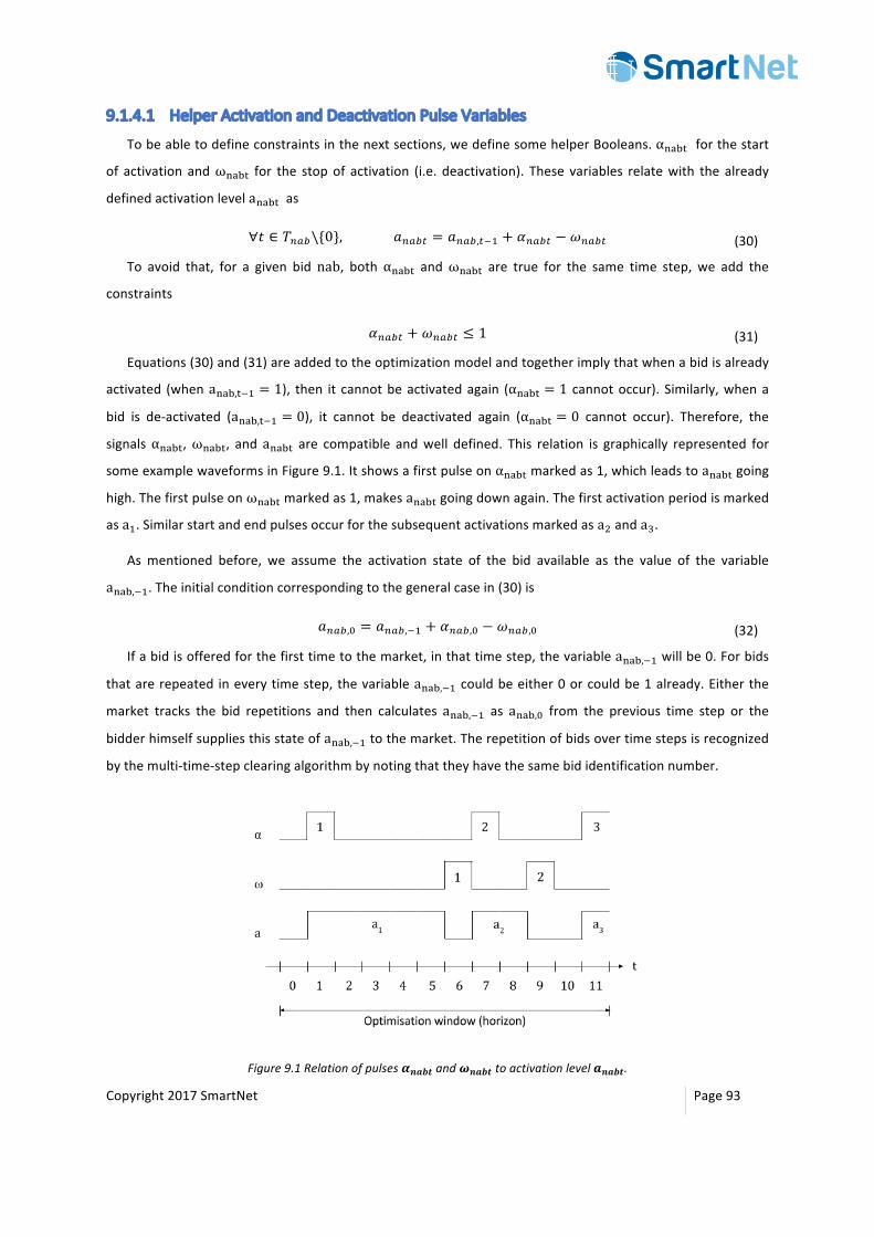
Copyright2017SmartNet Page93
9.1.4.1 HelperActivationandDeactivationPulseVariables
Tobeabletodefineconstraintsinthenextsections,wedefinesomehelperBooleans.αNOSTforthestart
of activationandωNOST for the stopof activation (i.e. deactivation). These variables relatewith the already
definedactivationlevelaNOSTas
∀𝑡 ∈ 𝑇*+´\{0},𝑎*+´l = 𝑎*+´,l�4 + 𝛼*+´l − 𝜔*+´l (30)
To avoid that, for a given bidnab, bothαNOST andωNOST are true for the same time step, we add the
constraints
𝛼*+´l + 𝜔*+´l ≤ 1 (31)
Equations(30)and(31)areaddedtotheoptimizationmodelandtogetherimplythatwhenabidisalready
activated (whenaNOS,T�4 = 1), then it cannotbeactivatedagain (αNOST = 1 cannotoccur). Similarly,whena
bid is de-activated (aNOS,T�4 = 0), it cannot be deactivated again (αNOST = 0 cannot occur). Therefore, the
signalsαNOST,ωNOST, andaNOST are compatible andwell defined. This relation is graphically represented for
someexamplewaveformsinFigure9.1.ItshowsafirstpulseonαNOSTmarkedas1,whichleadstoaNOSTgoing
high.ThefirstpulseonωNOSTmarkedas1,makesaNOSTgoingdownagain.Thefirstactivationperiodismarked
asa4.SimilarstartandendpulsesoccurforthesubsequentactivationsmarkedasaEandaF.
As mentioned before, we assume the activation state of the bid available as the value of the variable
aNOS,�4.Theinitialconditioncorrespondingtothegeneralcasein(30)is
𝑎*+´,3 = 𝑎*+´,�4 + 𝛼*+´,3 − 𝜔*+´,3 (32)
Ifabidisofferedforthefirsttimetothemarket,inthattimestep,thevariableaNOS,�4willbe0.Forbids
thatarerepeated ineverytimestep,thevariableaNOS,�4couldbeeither0orcouldbe1already.Eitherthe
market tracks the bid repetitions and then calculates aNOS,�4 as aNOS,3 from the previous time step or the
bidderhimselfsuppliesthisstateofaNOS,�4tothemarket.Therepetitionofbidsovertimestepsisrecognized
bythemulti-time-stepclearingalgorithmbynotingthattheyhavethesamebididentificationnumber.
Figure9.1Relationofpulses𝜶𝒏𝒂𝒃𝒕and𝝎𝒏𝒂𝒃𝒕toactivationlevel𝒂𝒏𝒂𝒃𝒕.
Copyright2017SmartNet Page94
9.1.4.2 Accept-All-Time-Steps-or-NoneConstraint
Whentheactorspecifies that thebid is ‘Accept-All-Time-Steps-or-None’, the followingconstraintwill
beset:
𝛿*+´µ = #𝑇*+´ (33)
where#𝑇*+´ isthebidhorizon(i.e.numberoftime-stepsintheQt-bid).Notethatall𝛿′𝑠areconstant
parametersandnotvariables.
9.1.4.3 RampingConstraints
Wesupposetherampingconstraintsareexactlythesameforeverytwoconsecutivetimestepsofthe
bid.Itholdsthat:
𝑞*+´,l ≤ 𝑞*+´,l�4 + 𝛥𝑞*+´ (ramp-uplimit) (34)
and
𝑞*+´,l ≥ 𝑞*+´,l�4 + 𝛥𝑞*+´ (ramp-downlimit) (35)
Note that 𝛥𝑞*+´ ≥ 0 and 𝛥𝑞*+´ ≤ 0. This can also be used to allow specification of the ramp
constraintsatthefirsttime-stepinthebid:
𝑞*+´,3 ≤ 𝑞*+´,�4 + 𝛥𝑞*+´ (36)
𝑞*+´,3 ≥ 𝑞*+´,�4 + 𝛥𝑞*+´ (37)
9.1.4.4 MaximumNumberofActivationsConstraint
Tobeabletocountthenumberofstartsandstopsofactivationsduringthebidtimespan,thevariables
αNOSTandωNOSTdefinedpreviouslyareused.Theconstraintfortheupperboundonthenumberofactivations
isthen
𝛼*+´l
l∈�ÉÊË
≤ 𝛼*+´ (38)
NotethatthelimitsαNOSandωNOSareonaperbidbasis,andarenotgloballyconstrainingallbidsofthe
bidder.
9.1.4.5 MinimumandMaximumDurationofActivationConstraint
As for the minimum duration, the following equation expresses, that whenever, for a certain τ = t −
δNOSÛ + 1,αNOSTis1(beginningofactivation),aNOSTwillbe1(active)foratleasttheδNOSÛ timeslotststartingat
τ = t − δNOSÛ + 1andendingatτ = t.
∀𝜏 ∈ 𝑡 − 𝛿*+´µ + 1 ,𝛼*+´,· ≤ 𝑎*+´,l (39)

Copyright2017SmartNet Page95
Notethattheconstraints(39) implythatforthefirsttime-step,t = 0,valuesofαNOS,Ü for δNOSÛ − 1time
stepsbeforet = 0stillhavetobeknown.Theycaneitherbebiddersuppliedorhavetoberememberedfrom
thesamebidintheprevioustimestep.Thelatterassumesthatthemarketclearingalgorithmwouldbeableto
trackonebid in subsequentdecision time-steps.This couldbedonebymaking thebid ID remain the same
between subsequent time steps. For the scopeof this document,we assume this extra informationwill be
availablesomehow,eitherrememberedbythemulti-stepclearingalgorithmorsuppliedbythebidderdirectly.
Therefore, thevaluesαNOS,Ü, ∀τ ∈ δNOSÛ + 1, … , −2, −1 areassumedtobeavailable.Theirdefaultvaluesat
start-upshouldbezero.
SettingδNOSÛ = 0leadstononeoftheconstraintsoftype(39)beinggenerated,whichisfine,butitisnota
usefulcase.SettingδNOSÛ = 1 leads tooneconstraintper timestep tbeinggeneratedαNOS,Ü ≤ aNOS,T.This is
alsofineandthiswillbethedefaultvalueforδNOSÛ whentheuserdoesnotexplicitlyspecifyavalue.
Asforthemaximumduration,theconditionthataNOS,Tshouldnotbe1anylongerthanδNOSconsecutive
timesteps,cansimplybeenforcedby:
𝑎*+´,·l·Ýl�ÞÉÊË
ß ≤ 𝛿*+´µ
(40)
Indeed,the left-handsideof (40) isasumofδNOSÛ
+ 1 termsandshouldsumuptoatmost δNOSÛ
socan
neverbeequaltoδNOSÛ
+ 1.
ThevaluesaNOS,Ü, ∀τ ∈ −δNOSÛ
, … , −2, −1 areassumedtobeavailable.
SettingδNOSÛ
= 0willnotallowanyaNOS,Ttobe1foranyt.Thiswilldisallowanyactivationofthebid,which
canbeusefulfortestingpurposes,butnototherwise.SettingδNOSÛ
= TNOS allowsactivationtolastaslongas
thebidhorizon,whichistakentobethedefaultiftheuserdoesnotspecifyδNOSÛ
explicitly.
9.1.4.6 MinimalDelayBetweenTwoActivations
Theequationsreflectingminimumdelaybetweentheendofanactivationandthebeginningofthenext
activationaresimilartotheonesforthelimitsonthewindowbetweenbeginningandendofactivationinthe
lastsection.Essentially,onereplacesαNOSTbyωNOST,δNOSÛ
byδNOSà
,δNOSÛ byδNOSà ,andaNOSTby1 − aNOST.
Thisgivesfortheminimumdelaybetweenendandbeginningofnextactivation
∀𝜏 ∈ 𝑡 − 𝛿*+´¶ + 1,… , 𝑡 : 𝜔*+´,· ≤ 1 − 𝑎*+´,l (41)
Itisinterestingtonotethatforamaximumdelaybetweenactivations,theconstraintwouldbe
1 − 𝑎*+´,·l·Ýl�ÞÉÊË
á ≤ 𝛿*+´
. (42)
Copyright2017SmartNet Page96
However,wecannotallowabiddertoimposeamaximumonthetimeofbeingnon-activesincethenthe
biddercouldexploit this trick to force themarket toactivatehisbid.Therefore, theaboveconstraint isnot
addedtothemodel.
Asexplainedbefore,thevaluesaNOS,Ü, ∀τ ∈ −δNOSà + 1, … , −2, −1 arealsoassumedtobeavailableand
alsodefaulttozero.ThevaluesaNOS,Ü, ∀τ ∈ −δNOSà
, … , −δNOSà arenotusedandmaynotbedefinedatall.
9.1.4.7 IntegralConstraint
Asmentionedbefore,themarketclearingalgorithmwillonlyacceptbidswithabidhorizonTNOSsmalleror
equaltotheoptimizationtimewindowT.Theintegralconstraintisformulatedas:
𝑒*+´) ≤ 𝑞*+´l ⋅ 𝛿𝑡l∈�ÉÊË
≤ 𝑒*+´)
(43)
Note that,q (power quantity) is inMWande (energy quantity) is inMWh.When the lower andupper
boundsareequal,asingleequalityconstraintresults.Asaspecialcase,whentheboundsaresettozero,the
integralconstraintguaranteesthattheasset(usuallyathermalorelectricalstorage)returnstoitsinitialvalue
attheendofthebid-horizon,oritsenergycontentremainswithinthepre-definedbounds.
9.1.4.8 ImplicationConstraint
TheimplicationconstraintisdefinedinamatrixINO ⊂ BNO×BNO.Itisformulatedas:
∀´å´æ 𝑏, 𝑏z ∈ 𝐼*+, 𝑎𝑎*+,´ ≤ 𝑎𝑎*+,´æ (44)
IfaaNO,S = 1thenaaNO,Sæ isforcedtobe1.IfaaNO,S = 0,thennothingisenforcedonaaNO,Sæ.Therefore,the
implicationb → bzholds.
9.1.4.9 ExclusiveChoiceConstraint
This limitation is setupby firstcreatingasublist lwithina listXNOofbid-identifiers,andthenwithin the
sublist,requiringthatonebidcanbeacceptedatmost.Thisisenforcedbythefollowingconstraint:
∀𝑙 ∈ 𝑋*+, 𝑎𝑎*+´´∈r
≤ 1 (45)
Also,thisconstraintcanonlybeenforced,bythebidder,betweenbidsatthesamenodeandbelongingto
thisbidder.
9.1.4.10 DeferabilityConstraintWedonotformulateanindependentconstraintfordeferability,sinceitcanbedonebysubmittingtheQt-
bidandthedifferentshiftedversionsofitandthenaddinganexclusive-choiceconstrainttoit,ensuringthatat
mostoneoftheshiftedversionsofthebidisaccepted.
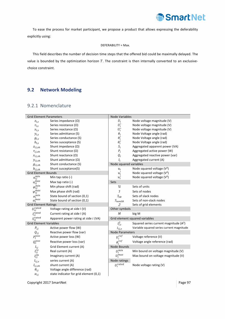
Copyright2017SmartNet Page97
Toeasetheprocess formarketparticipant,weproposeaproductthatallowsexpressingthedeferability
explicitlyusing:
DEFERABILITY=Max.
Thisfielddescribesthenumberofdecisiontimestepsthattheofferedbidcouldbemaximallydelayed.The
value isboundedby theoptimizationhorizon𝑇.Theconstraint is then internallyconverted toanexclusive-
choiceconstraint.
9.2 NetworkModeling
9.2.1 Nomenclature
GridElementParameters NodeVariables𝑧r,t Seriesimpedance(Ω) 𝑈) Nodevoltagemagnitude(V)𝑟r,t Seriesresistance(Ω) 𝑈)z Nodevoltagemagnitude(V)𝑥r,t Seriesreactance(Ω) 𝑈)∗ Nodevoltagemagnitude(V)𝑦r,t Seriesadmittance(S) 𝜃) NodeVoltageangle(rad)𝑔r,t Seriesconductance(S) 𝜃)z NodeVoltageangle(rad)𝑏r,t Seriessusceptance(S) 𝜃)∗ NodeVoltageangle(rad)𝑧)p,t| Shuntimpedance(Ω) 𝑆) Aggregatedapparentpower(VA)𝑟)p,t| Shuntresistance(Ω) 𝑃) Aggregatedactivepower(W)𝑥)p,t| Shuntreactance(Ω) 𝑄) Aggregatedreactivepower(var)𝑦)p,t| Shuntadmittance(Ω) 𝐼) Aggregatedcurrent(A)𝑔)p,t| Shuntconductance(S) Nodesquaredvariables𝑏)p,t| Shuntsusceptance(S) 𝑢) Nodesquaredvoltage(V²)
GridElementBounds 𝑢)z Nodesquaredvoltage(V²)𝑎)p()* Mintapratio(-) 𝑢)∗ Nodesquaredvoltage(V²)𝑎)p(+, Maxtapratio(-) Sets𝜑)p()* Minphaseshift(rad) 𝒰 Setsofunits𝜑)p(+, Maxphaseshift(rad) ℐ Setsofnodes𝛼r()* Stateboundofsection(0,1) ℐïð Setsofslacknodes𝛼r(+, Stateboundofsection(0,1) ℐ*Â*ïð Setsofnon-slacknodes
GridElementRatings 𝒥 Setsofgridelements𝑈)pk+lmn VoltageratingatsideI(V) Othersymbols𝐼)pk+lmn CurrentratingatsideI(A) 𝑀 bigM𝑆)pk+lmn Apparentpowerratingatside𝑖(VA) Gridelementsquaredvariables
GridElementVariables 𝐼r,tE Squaredseriescurrentmagnitude(A²)𝑃)p Activepowerflow(W) 𝑖)p,t Variablesquaredseriescurrentmagnitude𝑄)p Reactivepowerflow(var) NodeParameters𝑃rrÂtt Activepowerloss(W) 𝑈)
kmò Voltagereference(V)𝑄rrÂtt Reactivepowerloss(var) 𝜃)
kmò Voltageanglereference(rad)𝐼)p GridElementcurrent(A) NodeBounds𝐼)pkm Realcurrent(A) 𝑈)()* Minboundonvoltagemagnitude(V)𝐼)p)( Imaginarycurrent(A) 𝑈)(+, Maxboundonvoltagemagnitude(V)𝐼)p,t seriescurrent(A) Noderatings 𝐼)p,t| shuntcurrent(A) 𝑈)k+lmn Nodevoltagerating(V)𝜃)p Voltageangledifference(rad) 𝛼)p stateindicatorforgridelement(0,1)
Copyright2017SmartNet Page98
𝑎)p instantaneousvoltagetransformationratio(-)
𝜑)p phaseshift(rad)
9.2.2 Notation
With the exception of Yalmip [92] and CVX, common algebraic modelling languages only support real-
valued variables. Intermediately, complex variables will be used in derivations, but ultimately, real-valued
constraintsetsareformulated.NotethatquadraticrepresentationofSOCPconstraintsisused,butthesecan
beconvertedtothe2-normvectorrepresentation.
𝑥4E + 𝑥EE ≤ 𝑥FE, 𝑥F ≥ 0 𝑥4E + 𝑥EE ≤ 𝑥F
𝑥4𝑥E E
≤ 𝑥F (46)
Finally, a typographicdistinction ismadebetween scalar variables, e.g.Wij andmatrix variables, e.g.W.
Valued indexes are subscripted and stylized in a specific font, e.g. ‘i’, whereas descriptive indexes are
superscriptedandstylizedasnormaltext,e.g.‘s’.
9.2.3 PhysicsofPowerFlow
In power system modeling, the system is typically represented as a single-wire diagram. This
representationmatchesnicelywiththeconceptofmathematicalgraphs.Mathematicalgraphsarecomposed
of nodes/vertices/buses and edges/arcs/lines. To convert circuits tomathematical graphs, edgemodels for
conductingelementsaredeveloped.
Gridnodesandelementsareassignedindexesasfollows:
• Gridnodesi;j∈ ℐ = ℐïð ∪ ℐ*Â*ïð
• Slackbusnodesi∈ ℐïð
• Non-slackbusnodesi∈ ℐ*Â*ïð
• Gridelementsl,ij∈ 𝒥
Forsymmetricvariablesandparameters,theindexlispreferredtoijorji.
Nodesareconnected toeachother throughconductiveelements.Conductinggridelement technologies
include:overheadlines,undergroundcables,classictransformers,on-loadtap-changingtransformers,phase-
shiftingtransformers,switches,andbreakers.
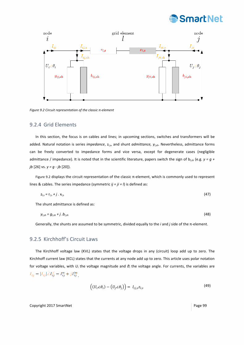
Copyright2017SmartNet Page99
Figure9.2Circuitrepresentationoftheclassicπ-element
9.2.4 GridElements
In this section, the focus ison cablesand lines; inupcoming sections, switchesand transformerswill be
added.Naturalnotation isseries impedance,zl,s,andshuntadmittance,yl,sh.Nevertheless,admittanceforms
can be freely converted to impedance forms and vice versa, except for degenerate cases (negligible
admittance/impedance).Itisnotedthatinthescientificliterature,papersswitchthesignofbl,sh(e.g.y=g+
jb[26]vs.y=g-jb[20]).
Figure9.2displaysthecircuitrepresentationoftheclassicπ-element,whichiscommonlyusedtorepresent
lines&cables.Theseriesimpedance(symmetricij=ji=l)isdefinedas:
zl,s=rl,s+j.xl,s (47)
Theshuntadmittanceisdefinedas:
yl,sh=gl,sh+j.bl,sh (48)
Generally,theshuntsareassumedtobesymmetric,dividedequallytotheiandjsideoftheπ-element.
9.2.5 Kirchhoff’sCircuitLaws
The Kirchhoff voltage law (KVL) states that the voltage drops in any (circuit) loop add up to zero. The
Kirchhoffcurrentlaw(KCL)statesthatthecurrentsatanynodeadduptozero.Thisarticleusespolarnotation
forvoltagevariables,withUi thevoltagemagnitudeandθi thevoltageangle.Forcurrents, thevariablesare
.
𝑈)∠𝜃) − 𝑈p∠𝜃p = 𝐼)p,t𝑧r,t (49)
Copyright2017SmartNet Page100
𝐼)p,t| = 𝑦)p,t| 𝑈)∠𝜃) (50)
𝐼p),t| = 𝑦p),t| 𝑈p∠𝜃p (51)
𝐼)p = 𝐼)p,t + 𝐼)p,t| (52)
𝐼p) = 𝐼p),t + 𝐼p),t| (53)
𝐼)p,t + 𝐼p),t = 0 (54)
HerewehaveOhm’slaw(49),thecurrenttotheshuntelements(50)-(51),andKirchhoff’scurrentlaw(52)-
(54) As is easily verified, Kirchhoff’s circuit laws are linear in voltage and current for constant impedances.
Notethatthisdescribesonlyonegridelement.Inmeshedgrids,KVLalsohastobeappliedinthemeshloops.
9.2.6 PowerFlow
As the purpose of the grid is to transport energy, stakeholders are interested in quantities of energy,
power,andcost.Power inACgridsconsideredascomplexrectangularvariableSij ,withPij theactivepower
andQijthereactivepower.Thecomplexconjugateoperatorisasuperscripted‘*’.EventhoughKLsappliedto
π-element results in a linear set of equations in current and voltage, adding equations tomodel (complex)
powerflowmakesthesetofequationsnonconvex:
𝑆)p = 𝑃)p + 𝑗𝑄)p = 𝑈)∠𝜃) 𝐼)p∗ (55)
Historically,OPFhasbeenbasedonthestaticapproximationtothepowerflowequations.Thismeansthat
inthepowerflowequations,therearenotimederivatives.
Voltage angles and reactive power do not have any useful meaning in the DC power flow domain.
Nevertheless,theequationsremainvalid(withθij=0;Qij=0;xl,s=0;bij,sh=0).
With interacting DC and AC grids, AC-DC converter models (for reactive power control of the AC-DC
converter)aretobeincluded.
9.2.7 Nodes
9.2.7.1 AnyNodeNodalaggregatepoweristhesumofallthepowersflowsawayfromnodeitoanyconnectednodej:
Voltageboundscanbeappliedatanynode.Theseusersuppliedboundscanbeusedtoreflectqualityof
supplystandardssuchasEN50160[93].
𝑈)()* ≤ 𝑈) ≤ 𝑈)(+, (56)
Copyright2017SmartNet Page101
9.2.7.2 NormalNodesComplex power flows Pi and Qi are determined by the units connected to the node. Voltage Ui∠𝜃)
consequentlyvaries.Someunitsmayhavecontrollerswhichregulatethevoltage.Commonly,thebusesthat
havegeneratorswithsuchcontrollers,arecalledPVbuses.Typically,then,reactivepowerdispatchischanged
tokeepthevoltagesteady.Moregenerally,activepowerdispatchcanalsobeadaptedtoregulatethevoltage.
9.2.7.3 VoltageanglereferencenodeOnenodeisrequiredtohaveavoltageanglereference:
𝜃)kmò ≤ 𝜃) ≤ 𝜃)
kmò (57)
Often,aslacknodeisusedinsteadofjustavoltageanglereferencebus.
9.2.7.4 SlacknodeAslacknodeisnotrequiredingeneral.However, inaradialgrid,theslacknodeisusedtorepresentthe
interaction with the external nodes, e.g. the transmission system. As the interface with the transmission
system is generally stronger than thedistribution grid connected to it, it is assumed that the slack bus can
support a large complex power flow at a fixed voltage. Conversely, in amicrogrid, one can choose not to
includeaslacknode,butmerelyavoltageanglereferencenode.
Itgenerallymakessensenottoconnectanyloadsorgeneratorsdirectlytothisnode,astheseunitsdonot
influencethepowerflowphysics.Ataslacknode,voltagemagnitudeandanglearefixed,buttherearefree
variables(slack)forthecomplexpowerflow:
𝜃)kmò ≤ 𝜃) ≤ 𝜃)
kmò (58)
𝑈)kmò ≤ 𝑈) ≤ 𝑈)
kmò (59)
−∞ ≤ 𝑃) ≤ ∞ (60)
−∞ ≤ 𝑄) ≤ ∞ (61)
9.2.8 ClassicPowerFlowFormulationsThepowerflowderivation inthissection isbasedontheclassicπ-elementrepresentationasdepicted in
Figure9.2.Threeformulationsarederived:rectangular,polarandDistFlow.Anyofthoseformulationscanbe
usedstraightawayinNLPsolvers.Commonly,thepolarformulationisimplemented.
9.2.8.1 PowerFlowRectangularThepowerbalanceandseriesandshuntcurrentsaredefinedastheproductofcomplexnumbers.
𝑃)p + 𝑗𝑄)p = 𝑈)∠𝜃) (𝐼)p,t| + 𝐼)p,t (62)
𝐼)p,t = ( 𝑈)∠𝜃) − 𝑈p∠𝜃p )𝑦r,t (63)
Copyright2017SmartNet Page102
𝐼)p,t| = 𝑈)∠𝜃) 𝑦)p,t| (64)
Combiningtheequationsaboveresultsintherectangularformulationofpowerflow:
𝑃)p + 𝑗𝑄)p = 𝑈)∠𝜃) 𝑈)∠𝜃) ∗ − 𝑈p∠𝜃p∗𝑦r,t∗ + 𝑈)E𝑦)p,t|∗ (65)
9.2.8.2 PowerFlowPolarThepowerflowequationsareformulatedinpolarformwithtrigonometricfunctions
𝜃)p = 𝜃) − 𝜃p (66)
𝑃)p = 𝑔r,t + 𝑔)p,t| 𝑈)E − 𝑔r,t𝑈)𝑈p cos 𝜃)p − 𝑏r,t𝑈)𝑈psin(𝜃)p) (67)
𝑄)p = − 𝑏r,t + 𝑏)p,t| 𝑈)E + 𝑏r,t𝑈)𝑈p cos 𝜃)p − 𝑔r,t𝑈)𝑈psin(𝜃)p) (68)
Thephaseangledifferenceoveranysectionisgenerallylimitedto90°:
−𝜋/2 ≤ 𝜃)()* ≤ 𝜃)p ≤ 𝜃)(+, ≤ 𝜋/2 (69)
9.2.8.3 PowerFlowDistFlowTheDistFlowreformulationprocesstakesthesquareofOhm’slaw,andderivesinanonconvexquadratic
equationinthevariablesofUi;Pij;QijandIij,s.
𝑈pE=𝑈)E − 2 𝑟r,t𝑃)p,t + 𝑥r,t𝑄)p,t + (𝑟r,tE + 𝑥r,tE )𝐼r,tE (70)
IntheDistFlowreformulation,thevoltageanglevariablesgetsubstitutedout.Thevoltagemagnitudesand
either end of a grid element can be related purely based on complex power flow and current magnitude
observations.Suchapproximationdoesnotchangetheresultsofthepowerflowinaradialgrid,asthevoltage
anglevariablescanstillbe recovered throughaprocesswhichgivesauniquesolution.However, inmeshed
gridsthisisnotthecaseduetovoltageangleconstraintapplyingtoanyloop.
Thepowerbalanceequationsarederivedasfollows:
Rectangularpowerflow
FeasibleSetI:(65)
Polarpowerflow
FeasibleSetII:(66)-(68)
DistFlowpowerflow
FeasibleSetIII:(70)
Copyright2017SmartNet Page103
0 ≤ 𝑃)p + 𝑃p) = 𝑃rrÂtt = 𝑃r,t|rÂtt + 𝑃r,trÂtt (71)
𝑄)p + 𝑄p) = 𝑄rrÂtt = 𝑄r,t|rÂtt + 𝑄r,trÂtt (72)
𝑃r,trÂtt = 𝑟r,t𝐼r,tE (73)
𝑄r,trÂtt = 𝑥r,t𝐼r,tE (74)
𝑃r,t|rÂtt = 𝑔r,t|𝑈)E (75)
𝑄r,t|rÂtt = −𝑏r,t|𝑈)E (76)
𝐼r,tE = (𝑃)pE + 𝑄)pE ) 𝑈)E (77)
NotethatUiand 𝐼)p,t onlyappearassquaredvariables.Thevoltageanglesshouldsatisfy:
𝜃)p = 𝜃) − 𝜃p = ∠(𝑈)∠θ))( 𝑈)∠θ) − 𝑧r,t𝐼)p,t)∗ (78)
𝜃)p = 0𝑚𝑜𝑑2𝜋rÂÂþ
(79)
Thevoltageangles inany loophavetoaddupto0mod2π,whichistriviallysatisfiedinaradialgridbut
whichrequiresadditionaltreatmentinmeshedgrids[44],[59].
9.2.8.4 OperationalEnvelopes
9.2.8.4.1 GridelementratingsBoundsonapparentpower,currentmagnitudeandvoltagemagnituderelatedtolines:
0 ≤ 𝑆)p ≤ 𝑆)pk+lmn (80)
0 ≤ 𝐼)p ≤ 𝐼)pk+lmn (81)
0 ≤ 𝑈) ≤ 𝑀 ∙ 𝑈)pk+lmn (82)
It isnotedthattheratingsdonotneedtobesymmetric(ij≠ ji),e.g.voltageratingsbeingdifferentwith
transformers. It is furthermorenoted that such voltage ratings, (which are generally always known, i.e. the
rating depends on the cablematerial, insulation level, etc.), can be used to derive generic bounds on the
voltages,butonlybyapplicationofabigM.
9.2.8.4.2 NoderatingsBoundsvoltagerelatedtonodes:
Gridelementratings
FeasibleSetIV:(80)-(82)

Copyright2017SmartNet Page104
0 ≤ 𝑈)()* ≤ 𝑈) ≤ 𝑈)(+, ≤ 𝑀 ∙ 𝑈)k+lmn (83)
Again, it is assumed that the voltage rating (voltage level) towhich nodes belong, is always known, i.e.
𝑈)k+lmn.Thiscanbeusedtodefineanupperboundonthevoltages,eveninabsenceofuser-suppliedbounds
UH"HN, 𝑈)(+,.
Noderatingandbound
FeasibleSetV:(83)

Copyright2017SmartNet Page105
9.3 ExtendedOPFFormulation
A commonly used model for the conducting elements is the π-element, as discussed in the previous
section,whichincludesaseriesimpedanceandshuntadmittancesateachendoftheline.Thisπ-elementcan
againbegeneralizedtoincludevoltagetransformation,phaseshiftingandswitching[94].Suchaformulation
will bedeveloped in thisworkand is referred to as the ‘extended symmetricπ-element’ representation, as
depictedinFigure9.3.Figure9.4furthermoredisplaysthecomplex-valuedgraphrepresentationcorresponding
totheextendedsymmetricπ-element.Finally,Figure9.5illustratesthereal-valuedgraphrepresentation.
Figure9.3Balancedπ-element-representationofaconductingelement.
Figure9.4Complex-valuedgraphrepresentationoftheextendedbalancedπ-element-representation.
Figure9.5Real-valuedgraphrepresentationsoftheextendedbalancedπ-element-representation.
Copyright2017SmartNet Page106
9.3.1 Transformer
Theeffectivetransformationratioisdefinedas:
𝑎)p = 𝑈)z
𝑈)∗ (84)
𝑎p) = 𝑈pz
𝑈p∗ (85)
Thisvoltagetransformationratioisboundedbyaminimumandmaximumvalue:
0 ≤ 𝑎)p()* ≤ 𝑎)p ≤ 𝑎)p(+, (86)
0 ≤ 𝑎p)()* ≤ 𝑎p) ≤ 𝑎p)(+, (87)
Tooperateataknownratio,thelower𝑎)p()*;𝑎p)()*andupperbounds𝑎)p(+,; 𝑎p)(+,aregivenequalvalues.
Minimumandmaximumphaseshiftaredefinedas:
0 ≤ 𝜑)p()* ≤ 𝜑)p ≤ 𝜑)p(+, (88)
0 ≤ 𝜑p)()* ≤ 𝜑p) ≤ 𝜑p)(+, (89)
𝜃)z = 𝜃)∗ + 𝜑)p (90)
𝜃pz = 𝜃p∗ + 𝜑p) (91)
Tooperateataknownphaseshift,thelower𝜑)p()*; 𝜑p)()*andupperbounds𝜑)p(+,; 𝜑p)(+,aregivenequal
values.Negativephaseshiftscanbehandledbyassigningtheshifttothecorrespondingsideoftheelement.A
negativephaseshiftfromitojcorrespondstoapositivephaseshiftfromjtoi.
Having a transformer at eachendallows you to: define the impedancemodel in any referencebase, to
separate voltage transformation and tap changing, and also to model tap changing at either side of the
transformer.
9.3.2 Switch
Foreachgridelementtohaveaninterpretablestatevariable,switchesarerequiredatbothends. Ifonly
oneswitchisused,powermaystill flowinthegridelementduetothecontributionsoftheshuntelements.
Onlyifswitchingoccursatbothsides,powerflowisguaranteedtobeinterrupted.
Stateαl=0meansbothswitchesareinopenpositionandthegridelementdoesnotconduct.Stateαl=1
means the switches are in closed position and the grid element does conduct. A disjunctive formulation is
developed,whichrequiresanupperboundonthevoltage(‘bigM’notationused).Instateαl=0,thevoltage
𝑈)∗isforcedto0,and𝑈)zisindependentfrom𝑈)∗.Instateαl=1,thevoltage𝑈)∗isnotforcedto0,butequality
of𝑈)zwith𝑈)∗isenforced.Forcing𝑈)∗to0issufficienttostoppowerflowthroughtheelement.
Copyright2017SmartNet Page107
𝛼r ∈ 0,1 (92)
0 ≤ 𝑈)∗ ≤ 𝑀 ∙ 𝛼r ∙ 𝑈)pk+lmn (93)
0 ≤ 𝑈p∗ ≤ 𝑀 ∙ 𝛼r ∙ 𝑈p)k+lmn (94)
0 ≤ 𝑈) − 𝑈)∗ ≤ 𝑀(1 − 𝛼r) ∙ 𝑈)pk+lmn (95)
0 ≤ 𝑈p −𝑈p∗ ≤ 𝑀(1 − 𝛼r) ∙ 𝑈p)k+lmn (96)
Ifaswitchisintheclosedposition,thevoltageanglesateitherendoftheswitchareequal.Iftheswitchis
open,thevoltageanglesarenotrelated.
−𝜋/2 ∙ 𝑀 ∙ (1 − 𝛼r) ≤ 𝜃) − 𝜃)∗ ≤ 𝜋/2 ∙ 𝑀(1 − 𝛼r) (97)
−𝜋/2 ∙ 𝑀 ∙ (1 − 𝛼r) ≤ 𝜃p − 𝜃p∗ ≤ 𝜋/2 ∙ 𝑀(1 − 𝛼r) (98)
−𝜋/2 ∙ 𝑀 ∙ 𝛼r ≤ 𝜃)z ≤ 𝜋/2 ∙ 𝑀 ∙ 𝛼r (99)
−𝜋/2 ∙ 𝑀 ∙ 𝛼r ≤ 𝜃pz ≤ 𝜋/2 ∙ 𝑀 ∙ 𝛼r (100)
Switchesaredynamicelementsandswitchingactionscontributetooperationalcosts.Thefollowingtypes
ofconstraintsareoftenconsideredinthiscontext:
• switchramprates
• switchcosts
• switchingrestrictedtocertaintimeslots
Tofixthestateoftheswitch,bounds𝛼r()*and𝛼r(+,canbeused:
0 ≤ 𝛼r()* ≤ 𝛼r ≤ 𝛼r(+, ≤ 1 (101)
Itisnotedthattheswitchpositiondoesnotneedtobeconsideredasavariable(throughfixingthebounds
andeliminationandsubstitution),eventhoughitcanbeusedasavariable.Nevertheless,thevariableswitch
formulationisalsousedinthemodellingofdiscretetransformertaps,seefurtherfordetailsonthis.
9.3.3 BranchFlowModelFormulation:DistFlow
9.3.3.1 Substitution
The complex current and voltage variables are replaced by squared current and voltage magnitude
variables.Therearenovariablesforcurrentorvoltageangles.
0 ≤ 𝑖)p,t = 𝐼)p,tE (102)
0 ≤ 𝑖)p = 𝐼)pE (103)
Copyright2017SmartNet Page108
0 ≤ 𝑢) = 𝑈)E (104)
0 ≤ 𝑢)z = 𝑈)zE (105)
0 ≤ 𝑢)∗ = 𝑈)∗E (106)
9.3.3.2 SOCPConvexFormulation
TheDistFlowequationsarereformulatedinthesquaredvariables:
0 ≤ 𝑃)p + 𝑃p) = 𝑃rrÂtt = 𝑃r,t|rÂtt + 𝑃r,trÂtt (107)
𝑄)p + 𝑄p) = 𝑄rrÂtt = 𝑄r,t|rÂtt + 𝑄r,trÂtt (108)
𝑃r,trÂtt = 𝑟r,t𝑖r,t (109)
𝑄r,trÂtt = 𝑥r,t𝑖r,t (110)
𝑃r,t|rÂtt = 𝑔r,t|𝑢)z (111)
𝑄r,t|rÂtt = −𝑏r,t|𝑢)z (112)
(𝑃)p,tE + 𝑄)p,tE ) ≤ 𝑢)z ∙ 𝑖r,t (113)
(𝑢)z − 𝑢pz) = −2(𝑟r,t𝑃)p,t + 𝑥r,t𝑄)p,t) + 𝑧r,tE∙ 𝑖r,t (114)
Withrespecttothenonconvexformulation,theconvexificationisthereplacementoftheequalitysymbol
in (77) by the inequality in (113), obtaining a second-order cone. Basically, (114) reflectsOhm’s law / KVL.
Furthermore,KCLisreflectedinthecomplexpowerbalanceequations(107)-(112)and(113)linksthepower,
voltageandcurrentvariablestogetherthroughtheconvexrelaxation.
Switchconstraintsarereformulatedinthesquaredvariables:
𝛼r ∈ 0,1 (115)
0 ≤ 𝑢)∗ ≤ 𝑀² ∙ 𝛼r ∙ (𝑈)pk+lmn)² (116)
0 ≤ 𝑢p∗ ≤ 𝑀² ∙ 𝛼r ∙ (𝑈)pk+lmn)² (117)
0 ≤ 𝑢) − 𝑢)∗ ≤ 𝑀²(1 − 𝛼r) ∙ (𝑈)pk+lmn)² (118)
0 ≤ 𝑢p − 𝑢p∗ ≤ 𝑀²(1 − 𝛼r) ∙ (𝑈)pk+lmn)² (119)
Thepowerflowthroughtheswitchthereforesatisfies:
SOCPDistFlow
FeasibleSetVI:(107)-(114)
Copyright2017SmartNet Page109
𝑃)pE + 𝑄)pE ≤ (𝐼)pk+lmn)² ∙ 𝑈)E ∙ 𝛼r (120)
This formulation effectively limits the total current magnitude 𝐼𝑖𝑗 to a maximum of 𝐼)pk+lmn , but doesn’t
require an explicit variable for the total current or total current magnitude. As the current rating isn’t
necessarily symmetrical, the equation is also considered for ji. This equation, after substitution, can be
formulatedinthenewvariablesas:
𝑃)pE + 𝑄)pE ≤ (𝐼)pk+lmn)² ∙ 𝑢) ∙ 𝛼r (121)
Thisconvexexpressionisarotatedsecond-ordercone.
Finally,thevoltagemagnitudetransformationisreformulatedinanexactmanneras:
(𝑎)p()*)²𝑢)∗ ≤ 𝑢)z ≤ (𝑎)p(+,)²𝑢)∗ (122)
(𝑎p)()*)²𝑢p∗ ≤ 𝑢pz ≤ (𝑎p)(+,)²𝑢p∗ (123)
It is noted that all the constraints only contain real-valued variables and parameters, therefore no
additional reformulation is required. In post-processing, complex-valued variables 𝐼)p, 𝑈)∠𝜃); 𝑆)p are again
obtained.
Thisrelaxationcanbepenalized,tomakesure𝑖)p,tand𝑢)zlayontheconesurface:
min𝑌%&�Â*'m, =1𝑛𝒥
𝑖)p,t(𝐼)pk+lmn)²r∈𝒥
(124)
Notethat𝑃)p,t or𝑄)p,t,also in(113),cannotbeeasilypenalizedduetotheirunknownsign.Theobjective
𝑌%&�Â*'m, is considered as a penalty in OPF problems with a wider scope, e.g. a multiperiod OPF with
operationalcostminimization.FormoreinsightsonthepenalizationoftheSOCPrelaxation,seesection4.4.5.
9.3.3.3 OperationalEnvelopes
Thevoltage, currentandcomplexpowerenvelopesare representable in the squaredvariablesby taking
thesquareoftheoriginalbounds.
(𝑈)()*)² ≤ 𝑢) ≤ (𝑈)(+,)² (125)
0 ≤ 𝑢)z ≤ 𝑀² ∙ (𝑈)pk+lmn)² (126)
0 ≤ 𝑖)p,t ≤ 𝑀² ∙ (𝐼)pk+lmn)² (127)
𝑃)pE + 𝑄)pE ≤ (𝑆)pk+lmn)² (128)
Switchinginsquaredvoltagemagnitudevariables(MILP)
FeasibleSetVII:(115)-(121)
Copyright2017SmartNet Page110
Notethattheapparentpowerflowboundoncomplexpowerflow(83)isacircularareaconstraint(𝑥4E +
𝑥EE ≤ 𝑟E), which is convex and representable as a SOCP constraint. Note also that by including expression
(127)anexplicitformulationforthecurrentboundisaddedtotheconstraintset.
Ultimately,theoverallfeasiblesetisderived:
9.3.3.4 Post-Processing
Theslackontheconvexificationisdefinedasfollows:
𝜖)p%&�Â*'m, = 𝑖)p,t ∙ 𝑢)z − 𝑃)p,tE − 𝑄)p,tE (129)
If𝜖)p%&�Â*'m, ≈ 0thenaphysicallymeaningfuloptimumisobtained.Duetonumericaleffects,theslackwill
notbe0exactly,andcanevenbeslightlynegative.If𝜖)p%&�Â*'m, ≉ 0thentheresultsarenotphysical.Slackon
theconvexificationimpliesartificiallyincreasedgridlosses.
Thevoltageangledifferencemustadduptozeroinanycycleinameshedgrid[59].
𝜃)pz = 𝜃)z − 𝜃pz = ∠ 𝑢)z − 𝑧r,t𝑆)p (130)
𝜃)p = 0𝑚𝑜𝑑2𝜋)p∈rÂÂþ
(131)
This condition is trivially satisfied in a radial grid, but the error has to be checkedwhen this formulation is
appliedtoameshedgrid.
Nopost-processing is required for𝑃)p, 𝑄)p, 𝛼r.Theoptimizedvariables𝑢), 𝑢)∗, 𝑢)z, 𝑖)p,t need tobemapped
back to the original variables 𝑈), 𝑈)∗, 𝑈)z, 𝜃), 𝜃)∗, 𝜃)z, 𝐼)p . A possible procedure for post-processing is the
following.Start fromslackbus,andsolvegridelementbygridelement,whilewalkingdownthe treeof the
network.
Itisnotedthatagenericpowerflowsolvercanalsobeusedtorecovertheresults.Powerflowsolverstake
as input the optimized dispatch of generators and loads (𝑃+;𝑄+) and the grid model (topology and
parameters),tocalculatevoltagesandcurrentsthroughoutthesystem.
ExtendedSOCPDistFlowenvelopes
FeasibleSetVIII:(122)-(124),(125)-(128)
ExtendedSOCPDistFlow
FeasibleSetIX:VI,VII,VIII
Copyright2017SmartNet Page111
9.3.4 BusInjectionModelFormulation
9.3.4.1 Substitution
Thecomplexvoltagevariablesarereplacedbycross-productsofnodevoltages.Therearenovariablesfor
voltageanglesandcurrent.Complex-valuedvariablesWijareelementsinthematrixW(notethatthisimplies
𝑖, 𝑗 ∈ ℕ).Theelementsareassignedtheproductsofvoltagevariables(𝑈)z∠𝜃)z)and(𝑈pz∠𝜃pz):
𝑊)p = 0 + 0𝑗∀𝑖𝑗 ∉ 𝒥 (132)
𝑊)p = 𝑈)z∠𝜃)z 𝑈pz∠𝜃pz∗∀𝑖𝑗 ∈ 𝒥 (133)
𝑊)p = (𝑈)z)² (134)
Nonexistent connections ij have Wij set to zero (132). Therefore, the matrixW is sparse if the degree of
meshednessofthenetworkislow.Notethatthis𝑛×𝑛matrixisHermitian𝑾 ∈ ℍ*,asitsatisfies𝑊)p = 𝑊p)∗.
ThisequalitybetweenthenaturalvoltagevariablesandWij(133)-(134)canalsobeformulatedasconstraints
onthismatrixvariable:
𝑾 ≽ 0 (135)
𝑟𝑎𝑛𝑘 𝑾 = 1 (136)
Thepositivesemi-definitenessisencodedas(135)andtherank-1requirementas(136).Thepowerbalance
canbeformulatedasfollows:
𝑆)p = (𝑦r,t + 𝑦)p,t|)∗𝑊)) − (𝑦r,t)𝑊)p (137)
Overall, this formulation then is a rank-constrained SDP problem. Only due to the rank constraint, the
problem isnonconvex.ToobtaintheSDPformulation, therankconstraint issimplydropped.Similar to Jabr
formulation[26],thevariables𝑅)p and𝑇)p areusedtomodeltherealandimaginarypartsofthevoltages,as
follows:
𝑊)p = 𝑅)p + 𝑗𝑇)p (138)
𝑅)p = 𝑅𝑒 𝑊)p = 𝑈)z𝑈pzcos(𝜃)pz ) (139)
𝑇)p = 𝐼𝑚 𝑊)p = 𝑈)z𝑈pzsin(𝜃)pz ) (140)
Itisnotedthatduetothesubstitution,thephase-shiftvariablesarenotexplicitintheconvexformulation.
Furthermore,voltageanglesrelatebythefollowingnonlinearequation:
𝜃)z − 𝜃pz = 𝑎𝑡𝑎𝑛2𝑇)p𝑅)p (141)
Aphaseangledifference(PAD)constraintcanthereforebeformulatedinthesevariablesasfollows:
Copyright2017SmartNet Page112
tan(𝜃)pz()*)𝑅)p ≤ 𝑇)p ≤ tan(𝜃)pz(+,)𝑅)p (142)
To obtain a tight convex hull, bounds implied on𝑅)p and 𝑇)p , through bounds on𝑊)),where𝑊)) are
derivedfrom(138)-(140),assuming𝜃)p ∈ [−𝜋/2, 𝜋/2]:
0 ≤ 𝑅)p ≤ 𝑀² ∙ 𝑈)pk+lmn𝑈p)k+lmn (143)
−𝑀² ∙ 𝑈)pk+lmn𝑈p)k+lmn ≤ 𝑇)p ≤ 𝑀² ∙ 𝑈)pk+lmn𝑈p)k+lmn (144)
Thevoltageboundsarereformulatedas
0 ≤ (𝑈)()*)² ≤ 𝑊)) ≤ (𝑈)(+,)² ≤ 𝑀E 𝑈)k+lmn ² (145)
9.3.4.2 SDPConvexRelaxation
Droprankconstraint(136)fromthefeasibleset.Ifthisrelaxedformulationsatisfies𝑟𝑎𝑛𝑘(𝑊) = 1inpost-
processing, the global optimum is found. The dropped rank constraint can be replaced with a rank
minimizationheuristicpenalty,basedonthetraceofthematrix[95]:
min 𝑡𝑟 𝑾 = 𝑊)))∈ℐ
(146)
min𝑌%&�Â*'m, =𝑊))
(𝑈)k+lmn)²)∈ℐ
(147)
9.3.4.3 SOCPConvexRelaxation
Thepositivesemi-definiteness(PSD)matrixconstraintcangenerallynotberepresentedinSOCPinanexact
manner.Anotherrepresentationisdevelopedforthesquaredvoltagemagnitude:
𝑊)p𝑊)p∗ = 𝑈)z∠𝜃)z 𝑈pz∠𝜃pz
∗ 𝑈)z∠𝜃pz
∗𝑈pz∠𝜃)z (148)
𝑊)p ² = 𝑊))𝑊pp (149)
Thisnonconvexequationisconsequentlyrelaxed:
𝑊)p ² ≤ 𝑊))𝑊pp (150)
The above constraint is a rotated second-order cone. Note that this formulation is equivalent to a PSD
constrainton2x2principalminors[15],[63](foralleffectivelinesij)intheoriginalmatrixW:
𝑊)) 𝑊)p
𝑊)p∗ 𝑊pp
≽ 0 𝑊)p ² ≤ 𝑊))𝑊pp(151)
SDPBIM
FeasibleSetX:(135),(137)
Copyright2017SmartNet Page113
Theresultingreal-valuedpowerflowequationsare:
𝑃)p = 𝑔r,t + 𝑔)p,t| 𝑊)) − 𝑔r,t𝑅)p − 𝑏r,t𝑇)p (152)
𝑄)p = −𝑏r,t + 𝑔)p,t| 𝑊)) + 𝑏r,t𝑅)p − 𝑔r,t𝑇)p (153)
𝑊))𝑊pp ≥ 𝑅)pE + 𝑇)pE (154)
Notethat𝑅)p = 𝑅p)but𝑇)p + 𝑇p) = 0.Therefore,thisrelaxationcanbepenalizedasfollows:
min𝑌%&�Â*'m, =1𝑛𝒥
𝑅)p)∈ℐ
(155)
9.3.4.4 Post-processing
Theslackontheconvexificationisdefinedasfollows:
𝜖)p%&�Â*'m, = 𝑊))𝑊pp − 𝑅)pE − (𝑇)pE) (156)
Nopost-processingisrequiredforPij,Qij,𝛼r.TheoptimizedvariablesRij,Tij,Wiineedtobemappedbackto
theoriginalvariablesUi,𝜃),Iij.Startfromslackbus,andcalculatelinebyline,whilewalkingdownthetreeof
thenetwork.
9.3.5 QCrelaxation
The Quadratic Convex or QC formulation is based on the use of convex hulls of the sine and cosine
function. Notation f(. ) is used to indicate the convex hull of the function f(.). Instead of variables being
bound by functions in equalities, variables can also be formulated as lying in the convex hull of nonlinear
functions.Astheoriginalfunctioniscontainedwithinthatconvexhull,throughthismethodology,arelaxation
oftheoriginalproblemisperformed.
𝑊))𝜖 (𝑈)z)² (157)
𝑅)p𝜖 𝑈)z𝑈pz cos(𝜃)pz ) (158)
𝑇)p𝜖 𝑈)z𝑈pz sin(𝜃)pz ) (159)
9.3.5.1 ConvexHullforCosineFunction
Tight convex hulls of sine, cosine and quadratic functions are derived in [30], [32]. The phase angle
differenceoveranysectionisconsideredlimitedto90°:
SOCPBIM
FeasibleSetXI:(152)-(154)
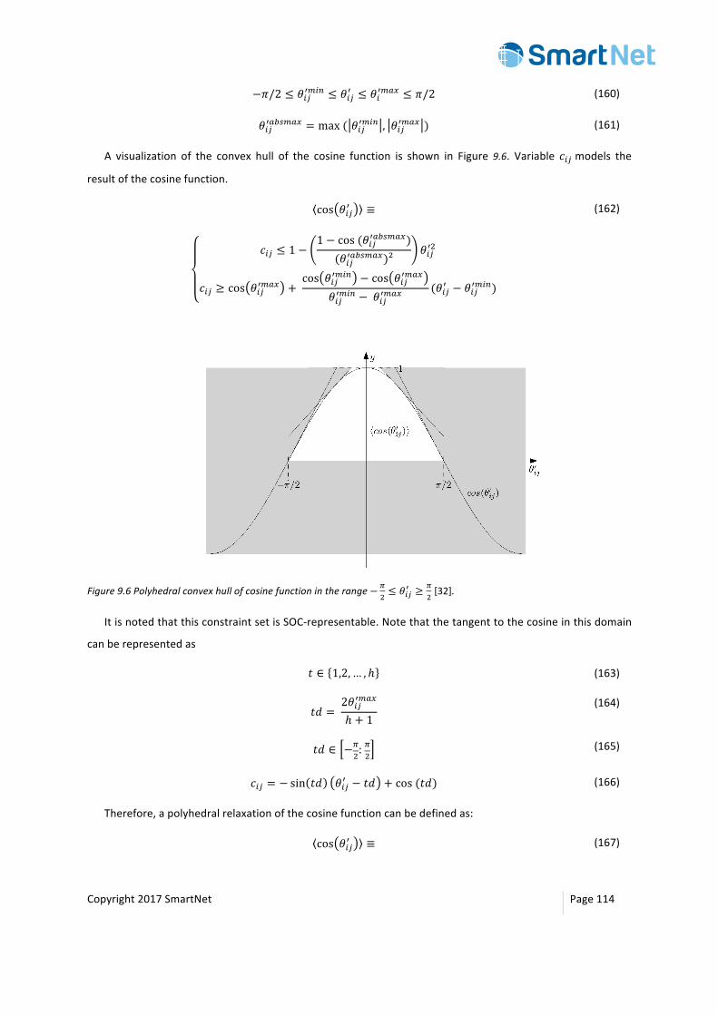
Copyright2017SmartNet Page114
−𝜋/2 ≤ 𝜃)pz()* ≤ 𝜃)pz ≤ 𝜃)z(+, ≤ 𝜋/2 (160)
𝜃)pz+´t(+, = max( 𝜃)pz()* , 𝜃)pz(+, ) (161)
A visualization of the convex hull of the cosine function is shown in Figure 9.6. Variable 𝑐)pmodels the
resultofthecosinefunction.
cos 𝜃)pz ≡
𝑐)p ≤ 1 −1 − cos(𝜃)pz+´t(+,)
(𝜃)pz+´t(+,)²𝜃)pzE
𝑐)p ≥ cos 𝜃)pz(+, + cos 𝜃)pz()* − cos 𝜃)pz(+,
𝜃)pz()* − 𝜃)pz(+,(𝜃)pz − 𝜃)pz()*)
(162)
Figure9.6Polyhedralconvexhullofcosinefunctionintherange− 4E≤ 𝜃)pz ≥
4E[32].
ItisnotedthatthisconstraintsetisSOC-representable.Notethatthetangenttothecosineinthisdomain
canberepresentedas
𝑡 ∈ 1,2, … , ℎ (163)
𝑡𝑑 =
2𝜃)pz(+,
ℎ + 1
(164)
𝑡𝑑 ∈ −4E:
4E
(165)
𝑐)p = − sin 𝑡𝑑 𝜃)pz − 𝑡𝑑 + cos(𝑡𝑑) (166)
Therefore,apolyhedralrelaxationofthecosinefunctioncanbedefinedas:
cos 𝜃)pz ≡ (167)
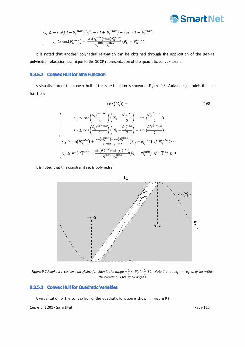
Copyright2017SmartNet Page115
𝑐)p ≤ − sin 𝑡𝑑 − 𝜃)pz(+, 𝜃)pz − 𝑡𝑑 +𝜃)pz(+, + cos(𝑡𝑑 −𝜃)pz(+,)
𝑐)p ≥ cos 𝜃)pz(+, + ab6 789
æ:8É �ab6 789æ:Ê;
789æ:8É�789
æ:Ê; (𝜃)pz − 𝜃)pz()*)
It is noted that another polyhedral relaxation can be obtained through the application of the Ben-Tal
polyhedralrelaxationtechniquetotheSOCPrepresentationofthequadraticconvexterms.
9.3.5.2 ConvexHullforSineFunction
Avisualizationoftheconvexhullofthesinefunction isshowninFigure9.7.Variable𝑠)p modelsthesine
function:
sin 𝜃)pz ≡
𝑠)p ≤ cos𝜃)pz+´t(+,
2𝜃)pz −
𝜃)pz(+,
2+ sin(
𝜃)pz+´t(+,
2)
𝑠)p ≥ cos𝜃)pz+´t(+,
2𝜃)pz +
𝜃)pz(+,
2− sin(
𝜃)pz+´t(+,
2)
𝑠)p ≥ sin 𝜃)pz()* + 6HN 789
æ:8É �6HN 789æ:Ê;
789æ:8É�789
æ:Ê; 𝜃)pz − 𝜃)pz()* 𝑖𝑓𝜃)pz()* ≥ 0
𝑠)p ≤ sin 𝜃)pz()* + 6HN 789
æ:8É �6HN 789æ:Ê;
789æ:8É�789
æ:Ê; 𝜃)pz − 𝜃)pz()* 𝑖𝑓𝜃)pz(+, ≥ 0
(168)
Itisnotedthatthisconstraintsetispolyhedral.
Figure9.7Polyhedralconvexhullofsinefunctionintherange− 4
E≤ 𝜃)pz ≥
4E[32].Notethat𝑠𝑖𝑛 𝜃)pz = 𝜃)pz onlylieswithin
theconvexhullforsmallangles.
9.3.5.3 ConvexHullforQuadraticVariables
AvisualizationoftheconvexhullofthequadraticfunctionisshowninFigure9.8.
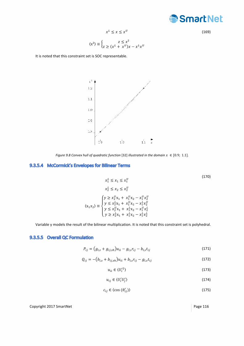
Copyright2017SmartNet Page116
𝑥< ≤ 𝑥 ≤ 𝑥=
x² ≡ 𝑧 ≤ 𝑥²𝑧 ≥ 𝑥< +𝑥= 𝑥 − 𝑥<𝑥=
(169)
ItisnotedthatthisconstraintsetisSOCrepresentable.
Figure9.8Convexhullofquadraticfunction[32]illustratedinthedomain𝑥 ∈ [0.9; 1.1].
9.3.5.4 McCormick’sEnvelopesforBilinearTerms
𝑥4< ≤ 𝑥4 ≤ 𝑥4=
𝑥E< ≤ 𝑥E ≤ 𝑥E=
x4𝑥E ≡
𝑦 ≥ 𝑥E=x4 + 𝑥4=xE − 𝑥4=𝑥E=
𝑦 ≤ 𝑥E<x4 + 𝑥4=xE − 𝑥4<𝑥E=
𝑦 ≤ 𝑥E=x4 + 𝑥4<xE − 𝑥4=𝑥E<
𝑦 ≥ 𝑥E<x4 + 𝑥4<xE − 𝑥4<𝑥E<
(170)
Variableymodelstheresultofthebilinearmultiplication.Itisnotedthatthisconstraintsetispolyhedral.
9.3.5.5 OverallQCFormulation
𝑃)p = 𝑔r,t + 𝑔)p,t| 𝑢)) − 𝑔r,t𝑟)p − 𝑏r,t𝑡)p (171)
𝑄)p = − 𝑏r,t + 𝑏)p,t| 𝑢)) + 𝑏r,t𝑟)p − 𝑔r,t𝑡)p (172)
𝑢)) ∈ 𝑈)zE (173)
𝑢)p ∈ 𝑈)z𝑈pz (174)
𝑐)p ∈ cos(𝜃)pz ) (175)
Copyright2017SmartNet Page117
𝑠)p ∈ sin(𝜃)pz ) (176)
𝑟)p ∈ 𝑢)p𝑐)p (177)
𝑡)p ∈ 𝑢)p𝑠)p (178)
Thetightertheanglebounds𝜃)pz()*; 𝜃)pz(+,areset,thetightertheformulation.
It is noted that the LPAC formulation [46] uses a convex-hull formulation of the cosine terms, in
combinationwithalinearizationofthesineterms.Apiecewiselinearizationofthisconvexhullisused,which
canbeconsideredasapolyhedralrelaxationofthequadratichullproposedhere.ThisLPACapproximationhas
astrongcorrelationwiththeNLPACformulationintransmissionsystems,andissuperiortothelinearized‘DC’
OPFformulation.
9.3.6 OPFApproximation:LinearDCFormulation
Thelinear‘DC’approximationisusedinSmartNettodescribethetransmissiongridphysicalconstraintsin
themarket-clearingalgorithm.
9.3.6.1 ModelFormulationTheDCformulationhasthefollowingassumptions.
• Branches can be considered lossless. In particular, if branch parameters 𝑟r,t, 𝑏r,t| and 𝑔r,t|are
negligible:
𝑦r,t = 1
𝑟r,t + 𝑗𝑥r,t≈
1𝑗𝑥r,t
,𝑏r,t| ≈ 0,𝑔r,t| ≈ 0 (179)
• Allbusvoltagemagnitudesareclosetoonep.u.
𝑈) ≈ 1 (180)
• Voltageangledifferencesacrossbranchesaresmall:
sin(𝜃) − 𝜃p + 𝜑)p) ≈ 𝜃) − 𝜃p + 𝜑)p (181)
• All theshuntelementscanbeconsideredasPQloadatconstantvoltage(e.g.nominalvoltage)and
addedtotheloadsvector.
Theapproximaterealpowerflowisthen:
QC
FeasibleSetXII:(158)-(178)
Copyright2017SmartNet Page118
𝑃)p ≈𝑎)p𝑥r,t
(𝜃) − 𝜃p + 𝜑)p) (182)
Asexpected,giventhelosslessassumption,asimilarderivationforthepowerinjectionatthetwoendsof
thelineleadsto𝑃)p = −𝑃p).
9.3.6.1.1 HVDCLinksTheHVDClinkscanbemodelledbytheuseofgeneratorswithoppositeinjection.ThelosseswithintheDC
cable,infirstapproximation,canbeneglected.
9.3.6.1.2 FACTSApproximationsIntheDCapproximation,all reactivepowercontroldevicesaredisregarded.Otherdevicesthatareused
onlyforspecificapplications(e.g.oscillationdampingorthe increaseofthetransmissioncapability)arealso
neglectedintheDCapproximation.Theonlydevicestobemodelledarethosewhodirectlyaffecttheactive
powerflow.Therearedifferentmodelswhichcanbeusedforeachsingledevice[96],[97].However,fromthe
pointofviewoftheDCmodel,theeffectoftheactivephaseshiftersistochangetheactivepowerflowofa
line,independentlyfromtheparticularmodelorcontrolscheme.Then,fortheDCmodelitisonlynecessaryto
knowtheactivepowerortheequivalentphaseshiftingasshownin[68],[71],[98].
9.3.6.2 IncludingLossesIncludingtheactivepowerlossesgivesabetteralignmentoftheACandDCmodels. Itwasshownthata
significantpartoftheerroroftheDCapproximationcomesfromnotconsideringthecontributionofnetwork
losses.
It ispossibletoimprovetheDCmodelincludingafirstapproximationofthelosses.Themainproblemto
include them is that it is necessary to know them before calculating the power flow. Either the losses are
alreadyknownfromconventionalvalues(basedontheoperationalexperience),oritisnecessarytocalculatea
completeACpowerflow,whichconsidersboththereactivepowerflowandtheresistanceofthelines.Once
thelossesareknown,itispossibletotakethemintoaccount,eitherbyincreasingtheloadsorbydecreasing
thegeneratorpowerinjections.
Ifonlythetotalamountoflossesisknown,itispossibletoscalealltheloadsorgenerators(usuallywitha
proportionalmultiplicationfactor).Ifthespecificlossesofeverysinglelineareknown,itispossibletoassign
the lossesof a linedirectly to the loadsor generatorsof the twobussesbetweenwhich the specific line is
connected[68],[99].
Thefinalproceduretoincludethelossesintheplatformcalculationswilldependalsoontheavailabledata
and on the structure of the platform itself. To show the effectiveness of the procedure five methods of
consideringthenetworklossesareaddressedhereandbetterdescribedintheAppendix.
Copyright2017SmartNet Page119
9.3.6.2.1 Method1-FlatLoss-ProfileMethod1usesaflatloss-profile,whichisaddedproportionallytotheload.Thevalueoftheflatloss-profile
parameterisselectedtoafixedvalue,e.g.2.5%(aboutthepercentageoflossesintheSpanishnetworkunder
normalconditions).
9.3.6.2.2 Method2-FlatLoss-ProfileRecomputedThepreviousmethod failswhen the lossesaredifferentwith respect the fixedvalue, in these cases the
errorisconcentratedparticularlyintheslackbus.Thenthelossesarerecomputedforeachparticularscenario.
9.3.6.2.3 Method3-LossesProportionaltoeachBusInmethod 3, the losses of each line in theDC power flow are assigned to the loads at the two busses
connectedbythelinewitha50%distribution.ThismethodshouldreducetheerroroftheDCapproximation,
sinceitconservesthegeographiclocationofthelosses.
9.3.6.2.4 Method4-ErrorProportionaltoeachGenItislikethemethod2,butinthiscasethelossesareassignedproportionallytothegeneratorproductions.
9.3.6.2.5 Method5-ErrorProportionaltoEachGenandGeneratorinHalfIt is like the method 2, but in this case the losses are assigned 50% proportionally to the generator
productionsand50%totheload.
9.3.6.3 ImprovedImpedanceCalculationItispossibletousethefollowingapproximationintheDCpowerflow:
𝑦r,t = −𝑗𝑥r,t
𝑟r,tE + 𝑥r,tE≈
1𝑗𝑥r,t
,𝑏r,t| ≈ 0,𝑔r,t| ≈ 0 (183)
This equation represents the Improved Impedance Calculation (IIC) and it should give a more accurate
behavior since it also takes the resistance of the lines into account.However, the achievable improvement
dependsonthestructureandtheparametersofthenetwork.
9.3.6.4 DCModelAccuracyItisimpossibletoevaluateaprioritheaccuracyoftheDCmodel:itdependsfromtheparticularnetwork
andscenarioconsidered.However,someconsiderationscanbemadeinordertoknowwheretheerrorscome
from[99].
• Neglectingthelossesbringsanerrorofafewpercent.However,ifthenetworkisbigandthereisonly
one slackbus, theerror in theproximityof the slackbus can increase considerably. Then it is necessary to
distributethelossestoallthenetworkbusses.
• Themaximumangledifferencebetweentwobussesisusually40°,thentheerrorsbetween and
isusuallylessthan8.6%.
• Ifthevoltagelimitsaretakenintherangeof0.75to1.4pu,themaximumerrorisabout44%.
( )qsin
q
Copyright2017SmartNet Page120
• Theerrorofneglectingtheresistanceofthelinesdependsonther/xratioofthelines.Forr/xratios
ofabout1/3theerrorisabout11%,whichincreasesforhigherratio.HoweverusuallytheerrorofaDCmodel
ismuchlowerandtheaccuracyoftheDCpowerflowisaround5%oftheACpowerflow,butinparticularlines
theerrorcangreatlyincrease[71].Inparticularifther/xratioissmallerthan0.25,thentheerrorinthepower
flowsacrossthelines,whenconsideringACandDCsolution,doesnotexceed5%forthevastmajorityoflines
[100]. This because usually the r/x ratio is very small and similar for all the lines, then the flows in theDC
modeldivide themselves in the samewayof theACmodel.Besides that, thevoltageandangledifferences
between two consecutive busses are usually low. These approximations are not true with particular non-
linearitiesoftheACmodel(e.g.voltagedependenceoftheload,effectsofshuntelements,differencesinhigh
meshednetwork…).Theseerrorscanbeusuallyneglectedforthemarketapplications[68].
9.3.7 OPFwithAdditionalModels
Additionalmodelsandtheirfeasiblesetsaredevelopedinthissection.
9.3.7.1 PartialSlackNodetoLinkDistFlowwithLinearizedOPF
In linearized ‘DC’ OPF, active power flow and voltage angles are represented, but reactive power and
voltagemagnitudesarenotmodelled.Therefore,tolinkthelinearized‘DC’formulation,usedfortransmission
gridmodeling, with the DistFlow formulation, used in distribution gridmodeling, a new slack node type is
definedattheircommoninterface:
𝑈)kmò ≤ 𝑈) ≤ 𝑈)
kmò (184)
−∞ ≤ 𝑄) ≤ ∞ (185)
Avoltageanglereferencenodecanstillbedefinedatanynodeinthemodelofthetransmissionsystem.
9.3.7.2 OLTCTransformerwithDiscreteSteps
An on-load tap changing (OLTC) transformer is already modelled in a continuous way using the
formulationsdevelopedinSection9.3.1.Often,tapchangershavealimitednumberofdiscretesettings,e.g.
𝑎)p ∈ {0.90, 0.92, . . . , 1.08, 1.10}.Suchintegralityconstraintisconsideredasa‘specialorderedsetoftype1’
(SOS1)constraint,aMILPformulationtechniquewhichmodelsstepwisefunctions.Oneadds,foreachpossible
tapsettingl,theswitchstatevariableαl:
𝛼r ∈ 0,1 (186)
𝛼rr
= 1 (187)
Copyright2017SmartNet Page121
For each tap,onealsoaddsa transformer to theoptimizationmodelwith a known tap𝑎)p()* = 𝑎)p(+, ∈
{0.90, 0.92, . . . , 1.08, 1.10}.All these transformersarevirtuallyput inparallel.TheSOS1constraintenforces
thatonlyoneofthosetransformerswillactuallybeused.Thefactthatthevaluesinthetapsethaveanorder
canbeexploitedbycertainsolvers.
9.3.7.3 ZIPLoadModels
Genericloadbehavior,definedbyareference𝑃+kmòisoftendescribedintermsofconstantimpedance(Z),
current(I)andpower(P)parts,respectivelythroughparameters𝑎+@%; 𝑎+A%; 𝑎+%%.
SuchZIPloadmodelis(foractivepower)formulatedasfollows:
0 ≤ 𝑎+@% ≤ 1; 0 ≤ 𝑎+A% ≤ 1; 0 ≤ 𝑎+%% ≤ 1 (188)
𝑎+@% +𝑎+A% +𝑎+%% = 1 (189)
𝑃+ = 𝑎+@%
=B=BCDE
E
+ 𝑎+A%=B=BCDE + 𝑎+
%% 𝑃+kmò
(190)
Here,Uuisthevoltagemagnitudeseenbytheunit,namelythevoltageofthenodeUitheunitisconnected
to (there exists a mapping of u to i). From this formulation, it can be immediately seen that the Z and P
componentsarecompatiblewiththeconvexifiedACOPFformulationspreviouslydeveloped.Therefore,with
𝑎+A% = 0, themodel is exact in those variables. Nevertheless, there is no variable representing the voltage
magnitudeUu in that set of variables, only a variable for (Uu)². An approximation𝑈+r)* ≈ 𝑈+ is developed
basedontheTaylorseriesintheneighborhoodof𝑈+kmò.
𝑈+r)* = 𝑈+kmò + 4
E=BCDE(𝑢+ − 𝑈+
kmò E) (191)
TheapproximatedZIPformulationthenbecomes:
𝑃+ = 𝑎+@%
+B=BCDE ²
+ 𝑎+A%=BF8É
=BCDE + 𝑎+
%% 𝑃+kmò
(192)
This formulation is linear in the squared voltagemagnitude variable𝑢+. It is noted that ZIPmodels are
inherently approximate in any case, as it abstracts behavior of individual consumers and distributed
generationunits.AnequivalentZIPformulationissometimesdevelopedforreactivepower.
9.3.7.4 RadialityEnforcementinReconfiguration
Ifthegridelementstatevariablesarefree,onecandevelopoptimizationformulationsforreconfiguration.
Acommonobjectiveforgridreconfigurationisminimizationofgrid(energy)losses.
min 𝑃rÂtt (193)
Copyright2017SmartNet Page122
It is noted that equivalent formulations exist to enforce the radiality [101], which could be more
computationallyefficient,dependingonthecase.Suchconstraintsetsinclude‘singlecommodityflow’,‘multi-
commodityflow’,and‘spanningtree’[101].Below,thespanningtreeformulationisillustrated.Gridelements
areeitheractive,inactive,ortheswitchstatescanbeoptimized(194).Onlylimitednumberofgridelements
are active at the same time, to satisfy a necessary condition for radiality: the number of lines equals the
number of nodesminus one (195). For each line, there is a parent node indicator variablewhich is binary
(196).Alinehasatmostoneparentnode(197)andifithasaparentnode,thenthelineisinitsonstate.Every
non-slacknodeisaparentnodeonce(198)-(199).
0 ≤ 𝛼r()* ≤ 𝛼r ≤ 𝛼r(+, ≤ 1 (194)
𝛼r = 𝑛ℐ − 1r∈𝒥
(195)
𝛽)p ∈ 0,1 , 𝛽p) ∈ 0,1 (196)
𝛽)p + 𝛽p) = 𝛼r (197)
∀𝑖 ∈ ℐn,ïð: 𝛽)p = 0 (198)
∀𝑖 ∈ ℐn,*Â*ïð: 𝛽)p = 1 (199)
As the binary nature of αl is already guaranteed due to the integrality constraint (194), the integrality
constraint(96)canberemoved.
9.3.7.5 UnitModelingApproaches
FrameworksforMILPandMISOCPunitmodels,forconvexmultiperiodOPF,aredevelopedin[102],[103].
Furthermore,volt-varcontrolcanbeincorporatedinthemodelsofinvertersorsynchronousmachines[102],
[104].
9.3.8 Networkmodelingformulationextra’s
9.3.8.1 Definitionatan2
atan2 is a variation on the arctangent function with two arguments instead of one. This allows to
distinguishthesignofbotharguments.
𝑎𝑡𝑎𝑛2 𝑦, 𝑥 = (200)
Copyright2017SmartNet Page123
arctan𝑦𝑥𝑖𝑓𝑥 > 0
arctan𝑦𝑥+ 𝜋𝑖𝑓𝑥 < 0𝑎𝑛𝑑𝑦 ≥ 0
arctan 𝑦, 𝑥 − 𝜋𝑖𝑓𝑥 > 0𝑎𝑛𝑑𝑦 > 0
+𝜋2𝑖𝑓𝑥 = 0𝑎𝑛𝑑𝑦 > 0
−𝜋2𝑖𝑓𝑥 = 0𝑎𝑛𝑑𝑦 < 0
𝑢𝑛𝑑𝑒𝑓𝑖𝑛𝑒𝑑𝑖𝑓𝑥 = 0𝑎𝑛𝑑𝑦 = 0
9.3.8.2 RotatedSOCP
The2-normrepresentationofarotatedSOCisthefollowing
𝑥4E + 𝑥EE ≤ 𝑥F𝑥G, 𝑥F ≥ 0, 𝑥G ≥ 0
2𝑥42𝑥E
𝑥F − 𝑥G≤ 𝑥F + 𝑥G
2𝑥4 E + 2𝑥E E + 𝑥F − 𝑥G E ≤ (𝑥F + 𝑥G)²
2𝑥4 E + 2𝑥E E + 𝑥FE − 2𝑥F𝑥G + 𝑥GE ≤ 𝑥FE + 2𝑥F𝑥G + 𝑥GE
(201)
Aquadraticconstraint 𝑥4 E + 𝑥E E ≤ 𝑥Fwith𝑥F ≥ 0canbewrittenassucharotatedSOCwith𝑥Gkmò ≤
𝑥G ≤ 𝑥Gkmò.
9.4 Illustration of power flow approximations and relaxations:calculationresults
This section describes the results obtained by the optimal power flow calculations using the different
optionsforapproximationorrelaxationdescribedabove.
9.4.1 ObjectiveTheobjective for the optimal power flowproblemsdealtwith in the case studies discussedbelow is to
determinetheminimalcurtailingcostwhilestillmaintainingthebranchpowerflowsandbusvoltageswithin
their respectiveratings.Theassumptionsof thecurtailment flexibility inthecasestudiesareassumedtobe
thefollowing:
• Theactivepowerofthegeneratorsinthenetworkcanbecurtailedupto50%ofitsinitialvalue.The
boundsonthereactivepoweroutputofthegeneratorsaresettobethereactiveoutputatapowerfactorof
0.8 at the initial, i.e. maximal, active power generation. The constraints on the generator power are
implementedasboxconstraintswiththeupperandlowerboundsofactiveandreactivepowerspecifyingthe
boxedges.
Copyright2017SmartNet Page124
• The curtailable loads can be curtailed up to 20% of their initial value. The curtailable loads are
assumedtohaveaconstantpowerfactor;hencetheirreactivepowerconsumptionisdependentontheactive
powerconsumption.
Theminimalcurtailmentcost(€)isexpressedas:
𝑲𝒄𝒐𝒔𝒕 = (𝒄𝒖𝒄𝒖𝒓𝒕,𝑷 𝑷𝒖 − 𝑷𝒖
𝒓𝒆𝒇 + 𝒄𝒖𝒄𝒖𝒓𝒕,𝑸 𝑸𝒖 − 𝑸𝒖
𝒓𝒆𝒇 )𝒖∈𝓤
(202)
TheobjectiveusedintheoptimizationproblemYcostisnormalizedasfollows:
𝑌�Âtl = 𝐾�Âtl
(𝑐+�+kl,%𝑃+
kmò + 𝑐+�+kl,P𝑄+
kmò)+∈𝒰 (203)
with𝑃+kmò and𝑄+
kmò the initial power (active and reactive) consumption of the𝑢 ∈ 𝒰 flexible units (here:
dispatchablegeneratorsandcurtailable loads).Curtailingcostsareassumedtobeequal foreachcurtailable
load and generator (𝑐+�+kl,% = 10€/MW curtailed). A curtailing cost is also applied for a change in reactive
poweroutputofthegenerators(𝑐+�+kl,P=10€/Mvaradapted).Itisnotedthatthiscostfunctionisconvex.
9.4.2 CaseStudiesTheOPFcalculationsareappliedondifferentcasestudies.Allcasestudiesbuildonanadaptationof the
Atlantidetestgrid,i.e.aMVdistributionnetworkprovidedbyENELDistribuzionethroughtheAtlantideproject
[105]. It is a typical radial distribution networkwhere commercial, residential and industrial customers are
connected.Theradialnetworkhas101AClinesconnectingthe100ACbuseswith15kVasratedvoltage.The
total lengthofthe lines is120.42km,divided inoverhead lines(53.32km)andcables(67.10km).Atotalof
128loadsareconnectedtothenetwork,dividedinresidential,commercialandindustrialloads.Inadditionto
this,28generatorsareconnectedtothenetwork,theyareeitherrotating(3windgeneratorsand3CHPs)or
static(22photovoltaicsolarpanelinstallations)generators.AschematicofthenetworkisshowninFigure9.9,
the generators are indicated as blue circles, the loads as greenhouse-shaped nodes. Someof the loads are
curtailable,theseareindicatedaslight-greenloads.
Threecase studiesweredefined: ‘undervoltage’, ‘overvoltage’and ‘overcurrent’.Dependingon thecase
study,thepowerdemandandgenerationofeachload/generatorisadaptedsothatthegridsuffersfrombus
voltagesbelowthevoltagelimit,abovethevoltagelimitand/orbranchpowersexceedingbranchratings,ifno
curtailingwouldbeapplied.Figure9.10showsthecalculatedbusvoltagesineachcasestudy,Figure9.11shows
the calculated branch powers, and Figure 9.12 shows the number of each type of constraint violation
(undervoltage,overvoltageorpowerlimitexcess).
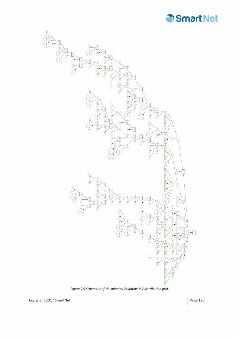
Copyright2017SmartNet Page125
Figure9.9SchematicoftheadaptedAtlantideMVdistributiongrid.
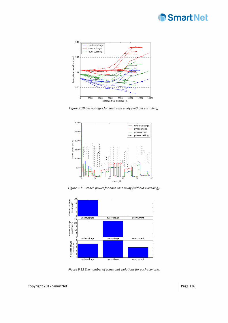
Copyright2017SmartNet Page126
Figure9.10Busvoltagesforeachcasestudy(withoutcurtailing).
Figure9.11Branchpowerforeachcasestudy(withoutcurtailing).
Figure9.12Thenumberofconstraintviolationsforeachscenario.
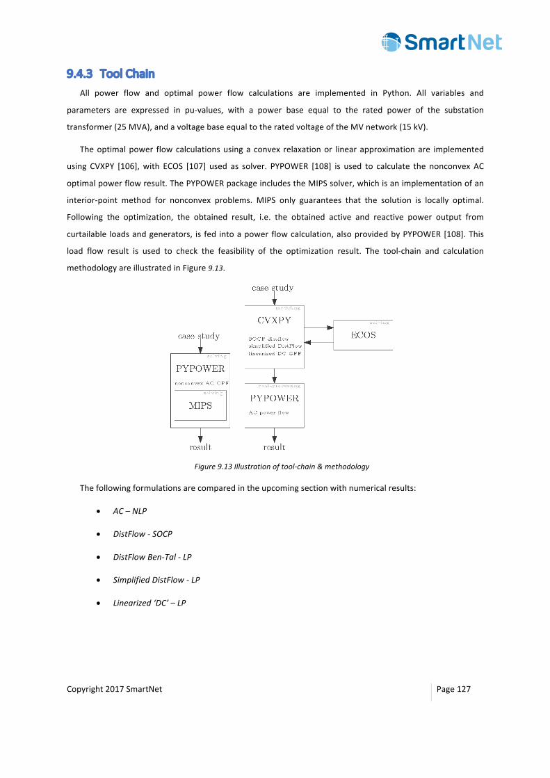
Copyright2017SmartNet Page127
9.4.3 ToolChainAll power flow and optimal power flow calculations are implemented in Python. All variables and
parameters are expressed in pu-values, with a power base equal to the rated power of the substation
transformer(25MVA),andavoltagebaseequaltotheratedvoltageoftheMVnetwork(15kV).
Theoptimalpower flowcalculationsusinga convex relaxationor linearapproximationare implemented
using CVXPY [106],with ECOS [107] used as solver. PYPOWER [108] is used to calculate the nonconvex AC
optimalpowerflowresult.ThePYPOWERpackageincludestheMIPSsolver,whichisanimplementationofan
interior-point method for nonconvex problems. MIPS only guarantees that the solution is locally optimal.
Following the optimization, the obtained result, i.e. the obtained active and reactive power output from
curtailable loadsandgenerators, is fed intoapowerflowcalculation,alsoprovidedbyPYPOWER[108].This
load flow result is used to check the feasibility of the optimization result. The tool-chain and calculation
methodologyareillustratedinFigure9.13.
Figure9.13Illustrationoftool-chain&methodology
Thefollowingformulationsarecomparedintheupcomingsectionwithnumericalresults:
• AC–NLP
• DistFlow-SOCP
• DistFlowBen-Tal-LP
• SimplifiedDistFlow-LP
• Linearized‘DC’–LP
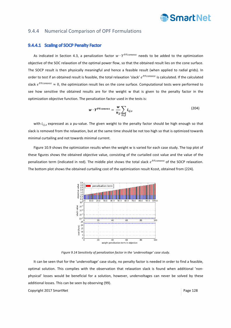
Copyright2017SmartNet Page128
9.4.4 NumericalComparisonofOPFFormulations
9.4.4.1 ScalingofSOCPPenaltyFactor
As indicated in Section 4.3, a penalization factor𝑤 ∙ 𝑌%&�Â*'m, needs to be added to the optimization
objectiveoftheSOCrelaxationoftheoptimalpowerflow,sothattheobtainedresultliesontheconesurface.
The SOCP result is then physicallymeaningful and hence a feasible result (when applied to radial grids). In
ordertotestifanobtainedresultisfeasible,thetotalrelaxation‘slack’𝜖%&�Â*'m,iscalculated.Ifthecalculated
slack𝜖%&�Â*'m, ≈ 0,theoptimizationresultliesontheconesurface.Computationaltestswereperformedto
see how sensitive the obtained results are for the weight w that is given to the penalty factor in the
optimizationobjectivefunction.Thepenalizationfactorusedinthetestsis:
𝒘 ∙ 𝒀𝑷𝑭𝒄𝒐𝒏𝒗𝒆𝒙 = 𝒘𝒏𝓙
𝒊𝒊𝒋,𝒔𝒍∈𝓙
(204)
with𝑖)p,texpressedasapu-value. Thegivenweight to thepenalty factor shouldbehighenough so that
slackisremovedfromtherelaxation,butatthesametimeshouldbenottoohighsothatisoptimizedtowards
minimalcurtailingandnottowardsminimalcurrent.
Figure10.9showstheoptimizationresultswhentheweightwisvariedforeachcasestudy.Thetopplotof
these figuresshowstheobtainedobjectivevalue,consistingof thecurtailedcostvalueandthevalueof the
penalization term(indicated in red).Themiddleplotshowsthe total slack𝜖%&�Â*'m,of theSOCPrelaxation.
ThebottomplotshowstheobtainedcurtailingcostoftheoptimizationresultKcost,obtainedfrom(224).
Figure9.14Sensitivityofpenalizationfactorinthe‘undervoltage’casestudy.
Itcanbeseenthatforthe‘undervoltage’casestudy,nopenaltyfactorisneededinordertofindafeasible,
optimal solution. This complies with the observation that relaxation slack is found when additional ’non-
physical’ losses would be beneficial for a solution, however, undervoltages can never be solved by these
additionallosses.Thiscanbeseenbyobserving(99).
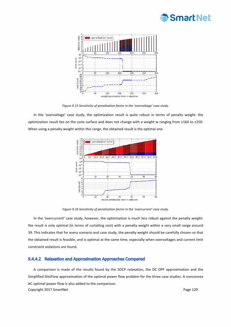
Copyright2017SmartNet Page129
Figure9.15Sensitivityofpenalizationfactorinthe‘overvoltage’casestudy.
In the ‘overvoltage’ case study, the optimization result is quite robust in terms of penalty weight: the
optimizationresultliesontheconesurfaceanddoesnotchangewithaweightwrangingfrom±164to±250.
Whenusingapenaltyweightwithinthisrange,theobtainedresultistheoptimalone.
Figure9.16Sensitivityofpenalizationfactorinthe‘overcurrent’casestudy.
Inthe‘overcurrent’casestudy,however,theoptimizationismuchlessrobustagainstthepenaltyweight:
theresultisonlyoptimal(intermsofcurtailingcost)withapenaltyweightwithinaverysmallrangearound
39.Thisindicatesthatforeveryscenarioandcasestudy,thepenaltyweightshouldbecarefullychosensothat
theobtainedresultisfeasible,andisoptimalatthesametime,especiallywhenovervoltagesandcurrentlimit
constraintviolationsarefound.
9.4.4.2 RelaxationandApproximationApproachesCompared
A comparison ismade of the results found by the SOCP relaxation, the DCOPF approximation and the
SimplifiedDistFlowapproximationoftheoptimalpowerflowproblemforthethreecasestudies.Anonconvex
ACoptimalpowerflowisalsoaddedtothecomparison.
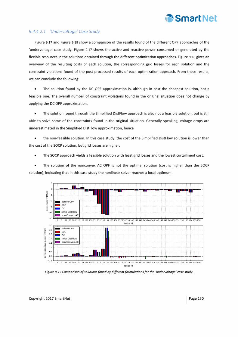
Copyright2017SmartNet Page130
9.4.4.2.1 ‘Undervoltage’CaseStudy
Figure9.17andFigure9.18showacomparisonoftheresultsfoundofthedifferentOPFapproachesofthe
‘undervoltage’ case study. Figure 9.17 shows the active and reactive power consumed or generated by the
flexibleresourcesinthesolutionsobtainedthroughthedifferentoptimizationapproaches.Figure9.18givesan
overview of the resulting costs of each solution, the corresponding grid losses for each solution and the
constraintviolations foundof thepost-processedresultsofeachoptimizationapproach.Fromtheseresults,
wecanconcludethefollowing:
• The solution found by the DCOPF approximation is, although in cost the cheapest solution, not a
feasibleone.Theoverall numberof constraint violations found in theoriginal situationdoesnot changeby
applyingtheDCOPFapproximation.
• ThesolutionfoundthroughtheSimplifiedDistFlowapproachisalsonotafeasiblesolution,butisstill
able to solve some of the constraints found in the original situation. Generally speaking, voltage drops are
underestimatedintheSimplifiedDistFlowapproximation,hence
• thenon-feasiblesolution.Inthiscasestudy,thecostoftheSimplifiedDistFlowsolutionislowerthan
thecostoftheSOCPsolution,butgridlossesarehigher.
• TheSOCPapproachyieldsafeasiblesolutionwithleastgridlossesandthelowestcurtailmentcost.
• The solution of the nonconvex AC OPF is not the optimal solution (cost is higher than the SOCP
solution),indicatingthatinthiscasestudythenonlinearsolverreachesalocaloptimum.
Figure9.17Comparisonofsolutionsfoundbydifferentformulationsforthe‘undervoltage’casestudy.
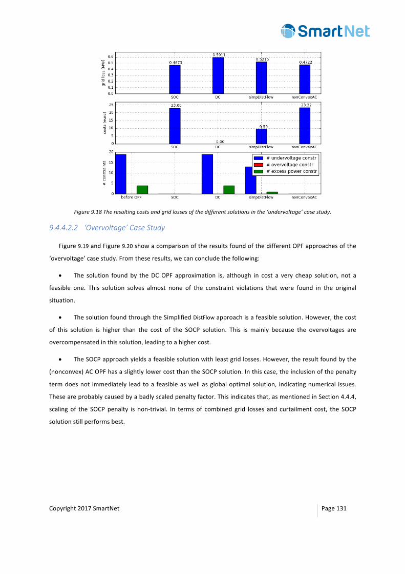
Copyright2017SmartNet Page131
Figure9.18Theresultingcostsandgridlossesofthedifferentsolutionsinthe‘undervoltage’casestudy.
9.4.4.2.2 ‘Overvoltage’CaseStudy
Figure9.19andFigure9.20showacomparisonoftheresultsfoundofthedifferentOPFapproachesofthe
‘overvoltage’casestudy.Fromtheseresults,wecanconcludethefollowing:
• The solution found by the DCOPF approximation is, although in cost a very cheap solution, not a
feasible one. This solution solves almost none of the constraint violations that were found in the original
situation.
• ThesolutionfoundthroughtheSimplifiedDistFlowapproachisafeasiblesolution.However,thecost
of this solution is higher than the cost of the SOCP solution. This is mainly because the overvoltages are
overcompensatedinthissolution,leadingtoahighercost.
• TheSOCPapproachyieldsafeasiblesolutionwithleastgridlosses.However,theresultfoundbythe
(nonconvex)ACOPFhasaslightlylowercostthantheSOCPsolution.Inthiscase,theinclusionofthepenalty
termdoesnot immediately lead toa feasibleaswellasglobaloptimal solution, indicatingnumerical issues.
Theseareprobablycausedbyabadlyscaledpenaltyfactor.Thisindicatesthat,asmentionedinSection4.4.4,
scaling of the SOCP penalty is non-trivial. In terms of combined grid losses and curtailment cost, the SOCP
solutionstillperformsbest.

Copyright2017SmartNet Page132
Figure9.19Comparisonofsolutionsfoundbydifferentformulationsforthe‘overvoltage’casestudy.
Figure9.20Theresultingcostsandgridlossesofthedifferentsolutionsinthe‘overvoltage’casestudy.
9.4.4.2.3 ‘Overcurrent’CaseStudy
Figure9.21andFigure9.22showacomparisonoftheresultsfoundofthedifferentOPFapproachesofthe
‘overcurrent’casestudy.Fromtheseresults,thefollowingcanbeconcluded:
• The solution found by the DCOPF approximation is, although in cost the cheapest solution, not a
feasibleone,asitfailstosatisfythebounds.
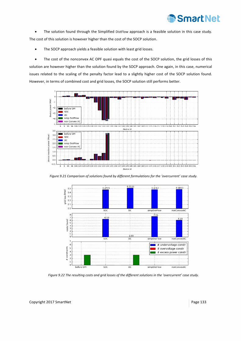
Copyright2017SmartNet Page133
• ThesolutionfoundthroughtheSimplifiedDistFlowapproachisafeasiblesolution inthiscasestudy.
ThecostofthissolutionishoweverhigherthanthecostoftheSOCPsolution.
• TheSOCPapproachyieldsafeasiblesolutionwithleastgridlosses.
• ThecostofthenonconvexACOPFquasiequalsthecostoftheSOCPsolution,thegridlossesofthis
solutionarehoweverhigherthanthesolutionfoundbytheSOCPapproach.Oneagain,inthiscase,numerical
issues related to the scalingof thepenalty factor lead to a slightly higher cost of the SOCP solution found.
However,intermsofcombinedcostandgridlosses,theSOCPsolutionstillperformsbetter.
Figure9.21Comparisonofsolutionsfoundbydifferentformulationsforthe‘overcurrent’casestudy.
Figure9.22Theresultingcostsandgridlossesofthedifferentsolutionsinthe‘overcurrent’casestudy.
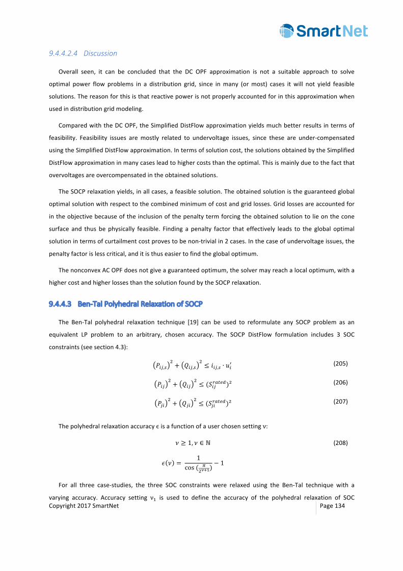
Copyright2017SmartNet Page134
9.4.4.2.4 Discussion
Overall seen, it can be concluded that the DC OPF approximation is not a suitable approach to solve
optimal power flow problems in a distribution grid, since inmany (ormost) cases it will not yield feasible
solutions.Thereasonforthisisthatreactivepowerisnotproperlyaccountedforinthisapproximationwhen
usedindistributiongridmodeling.
ComparedwiththeDCOPF,theSimplifiedDistFlowapproximationyieldsmuchbetterresults intermsof
feasibility. Feasibility issues aremostly related to undervoltage issues, since these are under-compensated
usingtheSimplifiedDistFlowapproximation.Intermsofsolutioncost,thesolutionsobtainedbytheSimplified
DistFlowapproximationinmanycasesleadtohighercoststhantheoptimal.Thisismainlyduetothefactthat
overvoltagesareovercompensatedintheobtainedsolutions.
TheSOCPrelaxationyields,inallcases,afeasiblesolution.Theobtainedsolutionistheguaranteedglobal
optimalsolutionwithrespecttothecombinedminimumofcostandgridlosses.Gridlossesareaccountedfor
intheobjectivebecauseoftheinclusionofthepenaltytermforcingtheobtainedsolutiontolieonthecone
surface and thus be physically feasible. Finding a penalty factor that effectively leads to the global optimal
solutionintermsofcurtailmentcostprovestobenon-trivialin2cases.Inthecaseofundervoltageissues,the
penaltyfactorislesscritical,anditisthuseasiertofindtheglobaloptimum.
ThenonconvexACOPFdoesnotgiveaguaranteedoptimum,thesolvermayreachalocaloptimum,witha
highercostandhigherlossesthanthesolutionfoundbytheSOCPrelaxation.
9.4.4.3 Ben-TalPolyhedralRelaxationofSOCP
The Ben-Tal polyhedral relaxation technique [19] can be used to reformulate any SOCP problem as an
equivalent LP problem to an arbitrary, chosen accuracy. The SOCP DistFlow formulation includes 3 SOC
constraints(seesection4.3):
𝑃)p,tE+ 𝑄)p,t
E≤ 𝑖)p,t ∙ 𝑢)z (205)
𝑃)pE+ 𝑄)p
E≤ (𝑆)pk+lmn)² (206)
𝑃p)E+ 𝑄p)
E≤ (𝑆p)k+lmn)² (207)
Thepolyhedralrelaxationaccuracyϵisafunctionofauserchosensettingν:
𝜈 ≥ 1, 𝜈 ∈ ℕ
𝜖 𝜈 = 1
cos( 4E\]^)
− 1
(208)
For all three case-studies, the three SOC constraints were relaxed using the Ben-Tal technique with a
varying accuracy. Accuracy setting ν4 is used to define the accuracy of the polyhedral relaxation of SOC
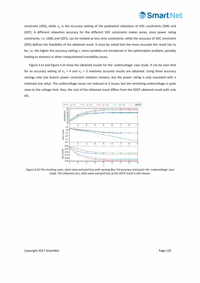
Copyright2017SmartNet Page135
constraint (205), while νE is the accuracy setting of the polyhedral relaxation of SOC constraints (206) and
(207). A different relaxation accuracy for the different SOC constraints makes sense, since power rating
constraints,i.e.(206)and(207),canbetreatedaslessstrictconstraints,whiletheaccuracyofSOCconstraint
(205)definesthefeasibilityoftheobtainedresult.Itmustbenotedthatthemoreaccuratetheresulthasto
be,i.e.thehighertheaccuracysettingν,morevariablesareintroducedintheoptimizationproblem,possibly
leadingtomemoryorothercomputationaltractabilityissues.
Figure9.23andFigure9.24showtheobtainedresultsforthe‘undervoltage’casestudy.Itcanbeseenthat
for an accuracy setting of ν4 = 4 and νE = 3 relatively accurate results are obtained. Using these accuracy
settings only one branch power constraint violation remains, but the power rating is only exceededwith a
relativelylowvalue.Theundervoltageissuesarereducedto3issues,buttheremainingundervoltageisquite
closetothevoltagelimit.Also,thecostoftheobtainedresultdiffersfromtheSOCPobtainedresultwithonly
4%.
Figure9.23Theresultingcosts,slackvalueandgridlosswithvaryingBen-Talaccuracysettingforthe‘undervoltage’case
study.Theobtainedcost,slackvalueandgridlossoftheSOCPresultisalsoshown.
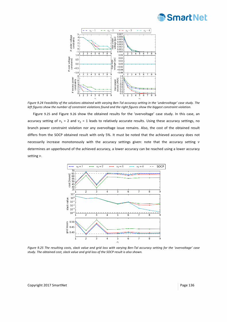
Copyright2017SmartNet Page136
Figure9.24FeasibilityofthesolutionsobtainedwithvaryingBen-Talaccuracysettinginthe‘undervoltage’casestudy.Theleftfiguresshowthenumberofconstraintviolationsfoundandtherightfiguresshowthebiggestconstraintviolation.
Figure 9.25 and Figure 9.26 show the obtained results for the ‘overvoltage’ case study. In this case, an
accuracy setting of𝜈4 = 2 and𝜈E = 1 leads to relatively accurate results. Using these accuracy settings, no
branch power constraint violation nor any overvoltage issue remains. Also, the cost of the obtained result
differs from the SOCPobtained resultwith only 5%. Itmust be noted that the achieved accuracy does not
necessarily increase monotonously with the accuracy settings given: note that the accuracy setting 𝜈
determinesanupperboundoftheachievedaccuracy,aloweraccuracycanbereachedusingaloweraccuracy
setting𝜈.
Figure9.25Theresultingcosts, slackvalueandgrid losswithvaryingBen-Talaccuracysetting for the ‘overvoltage’casestudy.Theobtainedcost,slackvalueandgridlossoftheSOCPresultisalsoshown.
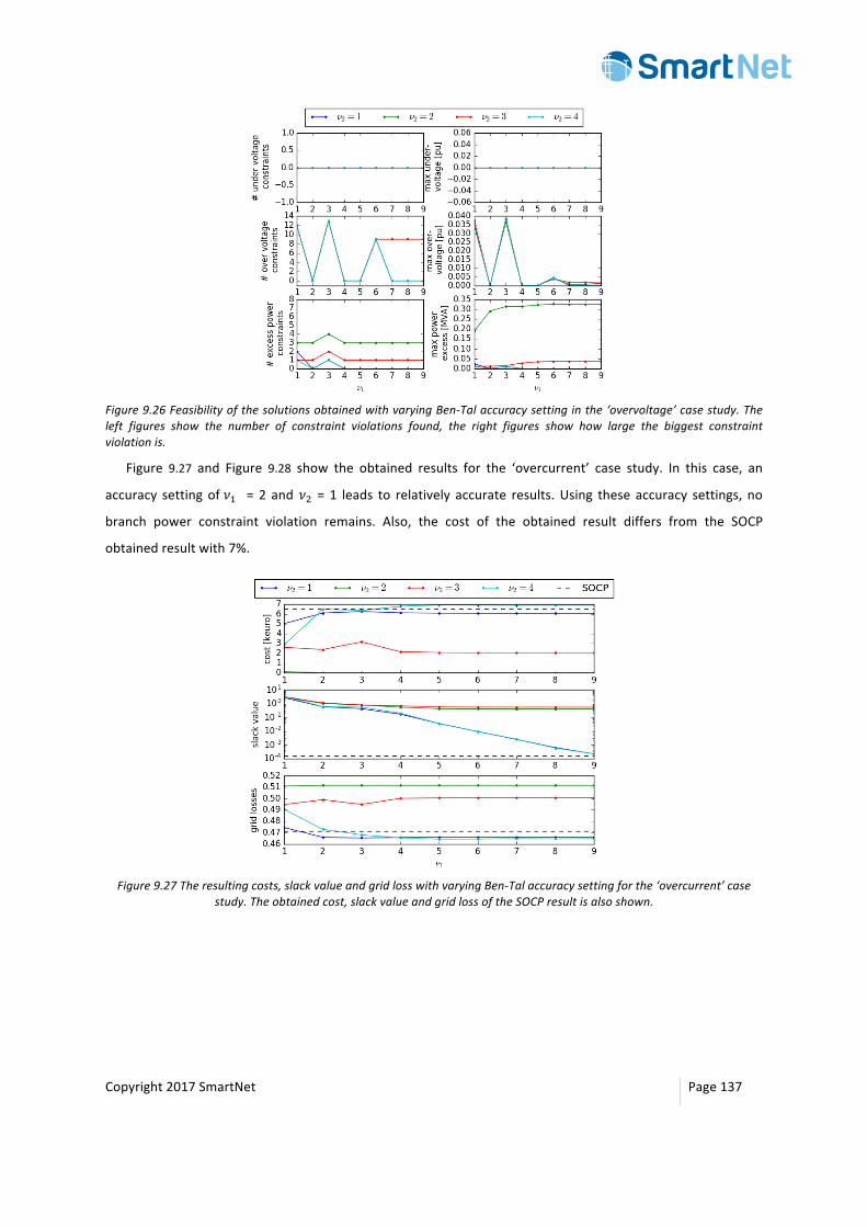
Copyright2017SmartNet Page137
Figure9.26FeasibilityofthesolutionsobtainedwithvaryingBen-Talaccuracysettinginthe‘overvoltage’casestudy.Theleft figures show the number of constraint violations found, the right figures show how large the biggest constraintviolationis.
Figure 9.27 and Figure 9.28 show the obtained results for the ‘overcurrent’ case study. In this case, an
accuracy settingof𝜈4 = 2 and𝜈E = 1 leads to relatively accurate results.Using these accuracy settings, no
branch power constraint violation remains. Also, the cost of the obtained result differs from the SOCP
obtainedresultwith7%.
Figure9.27Theresultingcosts,slackvalueandgridlosswithvaryingBen-Talaccuracysettingforthe‘overcurrent’case
study.Theobtainedcost,slackvalueandgridlossoftheSOCPresultisalsoshown.

Copyright2017SmartNet Page138
Figure9.28FeasibilityofthesolutionsobtainedwithvaryingBen-Talaccuracysettinginthe‘overcurrent’casestudy.Theleft figures show the number of constraint violations found, the right figures show how large the biggest constraintviolationis.
To conclude, in all tested case studies, relatively accurate Ben-Tal relaxation results are obtained with
relatively low accuracy settings. Accuracy settings of 𝜈4 and 𝜈E = 4 in all tested cases lead to acceptable
results.Thisimpliesthatwithouttheinclusionofmuchmoreextravariables,LPsolverscanbeusedtosolve
theSOCPproblemwithoutlosingtoomuchaccuracy.Aloweraccuracysettingmightbebetter,dependingon
thespecificcasestudy,sincetheaccuracysettingonlydeterminesanupperboundoftheachievedaccuracy.
9.4.5 VerificationStudyoftheInactiveConstraintsMethod
The inactive constraints method as network simplification method for transmission grid modeling is
illustratedinthischapter.Themethodisappliedtotheavailablenetworks,inordertofindtheinactivelines.
Tomaketheverificationmoregeneral,themethodisappliedtolargerangeofloadvalues.Theloadistreated
asavariablebetween10%and300%(dependingonthenetworkconsidered)ofthenominalvalue.Inthisway,
themethodisvalidatedindifferentloadingconditions.
InthecaseofSmartNet,alsothepossiblebalancingcomingfromtheflexibilitiesondistributionnetwork
shouldbeconsidered.Theproblemisthattherangeofvariationoftheseresourcesisnotknownatthisstage
oftheproject.
Theuseofmediumvoltageresourcescanreducetheuseofthehighvoltageresources.Theimpactofthe
medium voltage resources also depends on their position. However, the increase of distributed generation
shouldlimitthepowerflowinthetransmissionsystem,thenneglectingtheireffectshouldnotintroducegreat
errors.
Finally,we have to take into account thatwe are considering the balancingmarket. In thismarket, the
changesof theproduction/consumption,whicharecausedby relievingnetworkcongestionsandshort-term
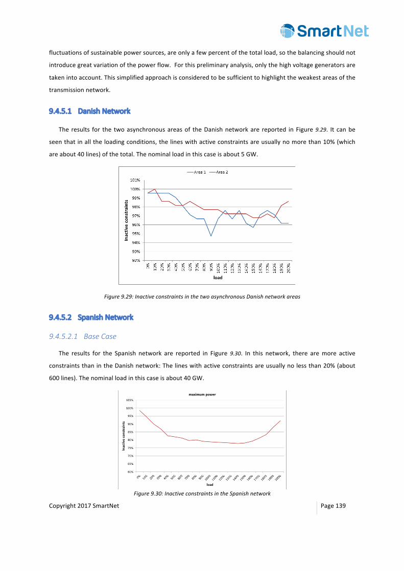
Copyright2017SmartNet Page139
fluctuationsofsustainablepowersources,areonlyafewpercentofthetotalload,sothebalancingshouldnot
introducegreatvariationofthepowerflow.Forthispreliminaryanalysis,onlythehighvoltagegeneratorsare
takenintoaccount.Thissimplifiedapproachisconsideredtobesufficienttohighlighttheweakestareasofthe
transmissionnetwork.
9.4.5.1 DanishNetwork
The results for the twoasynchronousareasof theDanishnetworkare reported inFigure9.29. It canbe
seenthatinalltheloadingconditions,thelineswithactiveconstraintsareusuallynomorethan10%(which
areabout40lines)ofthetotal.Thenominalloadinthiscaseisabout5GW.
Figure9.29:InactiveconstraintsinthetwoasynchronousDanishnetworkareas
9.4.5.2 SpanishNetwork
9.4.5.2.1 BaseCase
The results for the Spanish network are reported in Figure 9.30. In this network, there aremore active
constraintsthanintheDanishnetwork:Thelineswithactiveconstraintsareusuallynolessthan20%(about
600lines).Thenominalloadinthiscaseisabout40GW.
Figure9.30:InactiveconstraintsintheSpanishnetwork
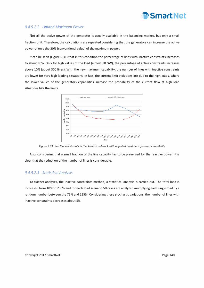
Copyright2017SmartNet Page140
9.4.5.2.2 LimitedMaximumPower
Not all the active power of the generator is usually available in the balancingmarket, but only a small
fractionofit.Therefore,thecalculationsarerepeatedconsideringthatthegeneratorscanincreasetheactive
powerofonlythe20%(conventionalvalue)ofthemaximumpower.
Itcanbeseen(Figure9.31)thatinthisconditionthepercentageoflineswithinactiveconstraintsincreases
toabout90%.Onlyforhighvaluesoftheload(almost80GW),thepercentageofactiveconstraintsincreases
above10%(about300lines).Withthenewmaximumcapability,thenumberoflineswithinactiveconstraints
arelowerforveryhighloadingsituations.Infact,thecurrentlimitviolationsareduetothehighloads,where
the lower values of the generators capabilities increase the probability of the current flow at high load
situationshitsthelimits.
Figure9.31:InactiveconstraintsintheSpanishnetworkwithadjustedmaximumgeneratorcapability
Also,consideringthatasmallfractionofthelinecapacityhastobepreservedforthereactivepower,itis
clearthatthereductionofthenumberoflinesisconsiderable.
9.4.5.2.3 StatisticalAnalysis
To furtheranalyses, the inactiveconstraintsmethod,astatisticalanalysis iscarriedout.Thetotal load is
increasedfrom10%to200%andforeachloadscenario50casesareanalyzedmultiplyingeachsingleloadbya
randomnumberbetweenthe75%and125%.Consideringthesestochasticvariations,thenumberoflineswith
inactiveconstraintsdecreasesabout5%
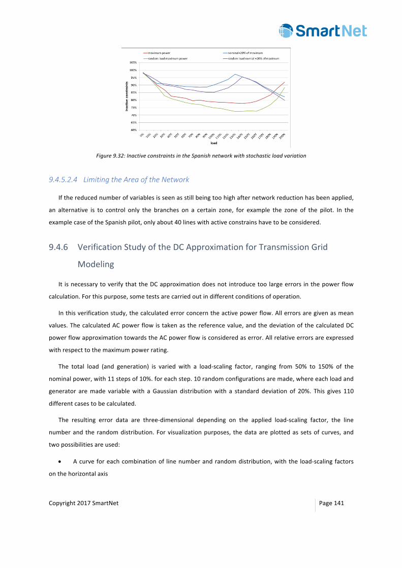
Copyright2017SmartNet Page141
Figure9.32:InactiveconstraintsintheSpanishnetworkwithstochasticloadvariation
9.4.5.2.4 LimitingtheAreaoftheNetwork
Ifthereducednumberofvariablesisseenasstillbeingtoohighafternetworkreductionhasbeenapplied,
an alternative is to control only the branches on a certain zone, for example the zone of the pilot. In the
examplecaseoftheSpanishpilot,onlyabout40lineswithactiveconstrainshavetobeconsidered.
9.4.6 VerificationStudyoftheDCApproximationforTransmissionGrid
Modeling
It isnecessarytoverifythattheDCapproximationdoesnot introducetoolargeerrors inthepowerflow
calculation.Forthispurpose,sometestsarecarriedoutindifferentconditionsofoperation.
Inthisverificationstudy,thecalculatederrorconcerntheactivepowerflow.Allerrorsaregivenasmean
values.ThecalculatedACpowerflowistakenasthereferencevalue,andthedeviationofthecalculatedDC
powerflowapproximationtowardstheACpowerflowisconsideredaserror.Allrelativeerrorsareexpressed
withrespecttothemaximumpowerrating.
The total load (and generation) is varied with a load-scaling factor, ranging from 50% to 150% of the
nominalpower,with11stepsof10%.foreachstep.10randomconfigurationsaremade,whereeachloadand
generator aremade variablewith a Gaussian distributionwith a standard deviation of 20%. This gives 110
differentcasestobecalculated.
The resulting error data are three-dimensional depending on the applied load-scaling factor, the line
numberand the randomdistribution.Forvisualizationpurposes, thedataareplottedas setsof curves,and
twopossibilitiesareused:
• Acurveforeachcombinationof linenumberandrandomdistribution,withthe load-scalingfactors
onthehorizontalaxis

Copyright2017SmartNet Page142
• Acurveforeachcombinationof load-scalingfactorandrandomdistribution,withthe linenumbers
onthehorizontalaxis
9.4.6.1 SpanishNetwork
StudyingtheSpanishnetworkhasshown,thattheerrorbetweentheDCandACpowerflow, intermsof
powerflowonthelines,islowonaverage.However,intheareaofthenetworkneartheslackbus,theerror
increases and become too relevant to be discarded (almost 500MW). In the following section reports the
resultofthemethodsintroduced.
9.4.6.1.1 Method1
Thefollowingprocedureisperformedforeachrandomsample:
1. Theloadsandgeneratorsareobtainedbytherandomprocedurepreviouslydescribed.
2. OneACPFisperformedtoobtainthelosses.
3. The losses are added proportionally to the generators. In this way, the balancing of the losses is
distributedbetweenallthegeneratorsandnotonlyintheslack.
4. TheACPFisrepeatedtakingintoaccountthenewgenerationprofilewiththelosses.
5. Flatlossesareaddedproportionallytotheload.
6. TheDCpowerflowiscomputed.
7. TheACandDCpowerflowarecompared.
Thevalueoftheflatloss-profileparameterisselectedto2.5%,whichisaboutthepercentageoflossesin
theSpanishnetworkundernormalconditions.
Themeanerrorinthiscaseis4.1MW.Themeanpercentageerror,computedwithrespectthepowerlimit
ofthelinesis1.3%.
Themeanerrorisquitelow,butitisnotacceptableinsomelines,inparticularwhenthereisahugeerror
neartheslackbus(Figure9.33;Figure9.34),sincetheslackhastobalancethelosses.
Theerrorisminimumwhentheloadandthelossesarenearthenominalcondition.Theyincreaseforthe
otherloadingconditions.Theerrorbecomesveryhighwhentheloadincreases(Figure9.34),sincethelosses
are quadraticwith respect the currents. It is clear that it is necessary to take into account, at least in first
approximation,thevalueofthelossestocomputetheexactvalueoftheload.
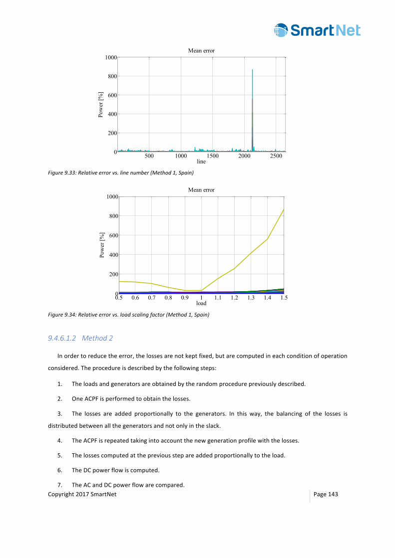
Copyright2017SmartNet Page143
Figure9.33:Relativeerrorvs.linenumber(Method1,Spain)
Figure9.34:Relativeerrorvs.loadscalingfactor(Method1,Spain)
9.4.6.1.2 Method2
Inordertoreducetheerror,thelossesarenotkeptfixed,butarecomputedineachconditionofoperation
considered.Theprocedureisdescribedbythefollowingsteps:
1. Theloadsandgeneratorsareobtainedbytherandomprocedurepreviouslydescribed.
2. OneACPFisperformedtoobtainthelosses.
3. The losses are added proportionally to the generators. In this way, the balancing of the losses is
distributedbetweenallthegeneratorsandnotonlyintheslack.
4. TheACPFisrepeatedtakingintoaccountthenewgenerationprofilewiththelosses.
5. Thelossescomputedatthepreviousstepareaddedproportionallytotheload.
6. TheDCpowerflowiscomputed.
7. TheACandDCpowerflowarecompared.
500 1000 1500 2000 25000
200
400
600
800
1000Mean error
line
Pow
er [%
]
0.5 0.6 0.7 0.8 0.9 1 1.1 1.2 1.3 1.4 1.50
200
400
600
800
1000Mean error
load
Pow
er [%
]
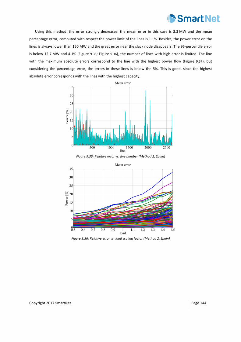
Copyright2017SmartNet Page144
Using this method, the error strongly decreases: the mean error in this case is 3.3MW and themean
percentageerror,computedwithrespectthepowerlimitofthelinesis1.1%.Besides,thepowererroronthe
linesisalwayslowerthan150MWandthegreaterrorneartheslacknodedisappears.The95-percentileerror
isbelow12.7MWand4.1%(Figure9.35;Figure9.36),thenumberof lineswithhigherroris limited.Theline
with the maximum absolute errors correspond to the line with the highest power flow (Figure 9.37), but
considering the percentage error, the errors in these lines is below the 5%. This is good, since the highest
absoluteerrorcorrespondswiththelineswiththehighestcapacity.
Figure9.35:Relativeerrorvs.linenumber(Method2,Spain)
Figure9.36:Relativeerrorvs.loadscalingfactor(Method2,Spain)
500 1000 1500 2000 25000
5
10
15
20
25
30
35Mean error
line
Pow
er [%
]
0.5 0.6 0.7 0.8 0.9 1 1.1 1.2 1.3 1.4 1.50
5
10
15
20
25
30
35Mean error
load
Pow
er [%
]
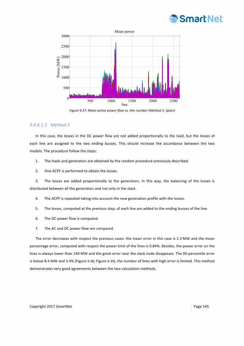
Copyright2017SmartNet Page145
Figure9.37:Meanactivepowerflowvs.linenumber(Method2,Spain)
9.4.6.1.3 Method3
In this case, the losses in theDCpower flowarenotaddedproportionally to the load,but the lossesof
each line are assigned to the two ending busses. This should increase the accordance between the two
models.Theprocedurefollowthesteps:
1. Theloadsandgeneratorsareobtainedbytherandomprocedurepreviouslydescribed.
2. OneACPFisperformedtoobtainthelosses.
3. The losses are added proportionally to the generators. In this way, the balancing of the losses is
distributedbetweenallthegeneratorsandnotonlyintheslack.
4. TheACPFisrepeatedtakingintoaccountthenewgenerationprofilewiththelosses.
5. Thelosses,computedatthepreviousstep,ofeachlineareaddedtotheendingbussesoftheline.
6. TheDCpowerflowiscomputed.
7. TheACandDCpowerflowarecompared.
Theerrordecreaseswithrespectthepreviouscases:themeanerrorinthiscaseis2.3MWandthemean
percentageerror,computedwithrespectthepowerlimitofthelinesis0.84%.Besides,thepowererroronthe
linesisalwayslowerthan140MWandthegreaterrorneartheslacknodedisappears.The95-percentileerror
isbelow8.4MWand3.4%(Figure9.38;Figure9.39),thenumberoflineswithhigherrorislimited.Thismethod
demonstratesverygoodagreementsbetweenthetwocalculationmethods.
500 1000 1500 2000 25000
500
1000
1500
2000
2500
3000Mean power
line
Pow
er [M
W]
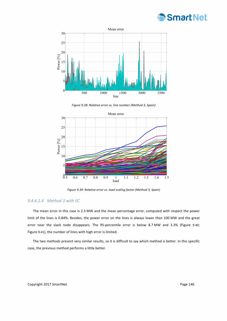
Copyright2017SmartNet Page146
Figure9.38:Relativeerrorvs.linenumber(Method3,Spain)
Figure9.39:Relativeerrorvs.loadscalingfactor(Method3,Spain)
9.4.6.1.4 Method3withIIC
Themeanerrorinthiscaseis2.3MWandthemeanpercentageerror,computedwithrespectthepower
limitofthe lines is0.84%.Besides,thepowererroronthelines isalways lowerthan100MWandthegreat
error near the slack node disappears. The 95-percentile error is below 8.7MW and 3.3% (Figure 9.40;
Figure9.41),thenumberoflineswithhigherrorislimited.
Thetwomethodspresentverysimilarresults,soitisdifficulttosaywhichmethodisbetter.Inthisspecific
case,thepreviousmethodperformsalittlebetter.
500 1000 1500 2000 25000
5
10
15
20
25
30Mean error
line
Pow
er [%
]
0.5 0.6 0.7 0.8 0.9 1 1.1 1.2 1.3 1.4 1.50
5
10
15
20
25
30Mean error
load
Pow
er [%
]
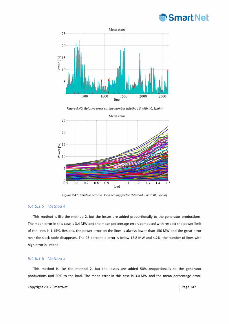
Copyright2017SmartNet Page147
Figure9.40:Relativeerrorvs.linenumber(Method3withIIC,Spain)
Figure9.41:Relativeerrorvs.loadscalingfactor(Method3withIIC,Spain)
9.4.6.1.5 Method4
Thismethod is like themethod2,but the lossesareaddedproportionally to thegeneratorproductions.
Themeanerrorinthiscaseis3.4MWandthemeanpercentageerror,computedwithrespectthepowerlimit
ofthelinesis1.15%.Besides,thepowererroronthelinesisalwayslowerthan150MWandthegreaterror
neartheslacknodedisappears.The95-percentileerrorisbelow12.8MWand4.2%,thenumberoflineswith
higherrorislimited.
9.4.6.1.6 Method5
This method is like the method 2, but the losses are added 50% proportionally to the generator
productions and 50% to the load. Themean error in this case is 3.0MW and themean percentage error,
500 1000 1500 2000 25000
5
10
15
20
25Mean error
line
Pow
er [%
]
0.5 0.6 0.7 0.8 0.9 1 1.1 1.2 1.3 1.4 1.50
5
10
15
20
25Mean error
load
Pow
er [%
]
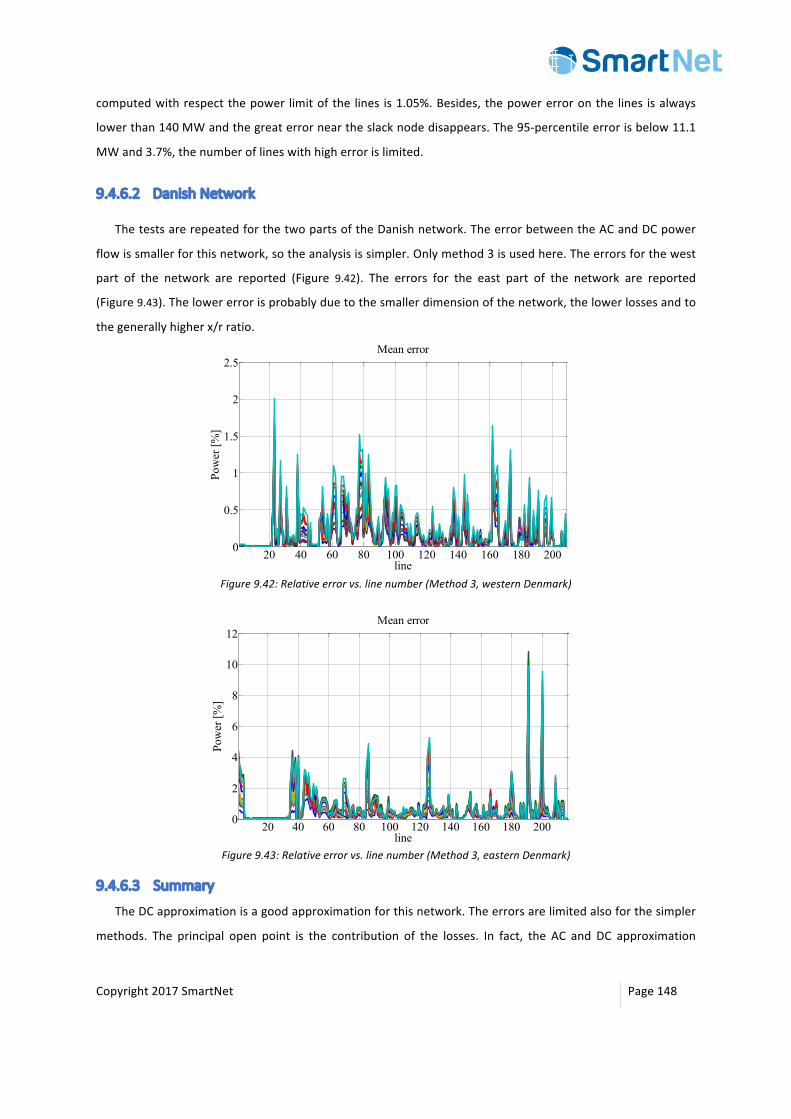
Copyright2017SmartNet Page148
computedwithrespectthepower limitofthe lines is1.05%.Besides,thepowererroronthe lines isalways
lowerthan140MWandthegreaterrorneartheslacknodedisappears.The95-percentileerrorisbelow11.1
MWand3.7%,thenumberoflineswithhigherrorislimited.
9.4.6.2 DanishNetwork
ThetestsarerepeatedforthetwopartsoftheDanishnetwork.TheerrorbetweentheACandDCpower
flowissmallerforthisnetwork,sotheanalysisissimpler.Onlymethod3isusedhere.Theerrorsforthewest
part of the network are reported (Figure 9.42). The errors for the east part of the network are reported
(Figure9.43).Thelowererrorisprobablyduetothesmallerdimensionofthenetwork,thelowerlossesandto
thegenerallyhigherx/rratio.
Figure9.42:Relativeerrorvs.linenumber(Method3,westernDenmark)
Figure9.43:Relativeerrorvs.linenumber(Method3,easternDenmark)
9.4.6.3 Summary
TheDCapproximationisagoodapproximationforthisnetwork.Theerrorsarelimitedalsoforthesimpler
methods. The principal open point is the contribution of the losses. In fact, the AC and DC approximation
20 40 60 80 100 120 140 160 180 2000
0.5
1
1.5
2
2.5Mean error
line
Pow
er [%
]
20 40 60 80 100 120 140 160 180 2000
2
4
6
8
10
12Mean error
line
Pow
er [%
]

Copyright2017SmartNet Page149
return thesameresultsonly if the lossesarecorrectly taken intoaccount.Thereareprincipally twoway to
takeintoaccountthelossesintheprojectframework:
• Thebalancingmarketsimulatesthenetworkcondition inthereal-timemarket.Thenthe inputdata
(profiles of load and generators) should already take into account the losses. Then it is possible to add the
losses in the DC approximation with different methods (proportionally to the load or to the generation).
However, since the AC power flow is not performed it ismore difficult to associate the losses to the lines
(futureinvestigation).
• The input data does not take into account the losses (for example if the data are fromday ahead
marketanditdoesnottakeintoaccountthelosses).Inthiscase,itisnotnecessarytoaddthelossesintheDC
formulation.
Copyright2017SmartNet Page150
9.5 MathematicalFormulationofMarketClearing
9.5.1 CouplingofPhysicsandEconomics
We startwith thephysical apparent-powerequilibrium. The following constraint expresses that𝑆*l, the
totalabsoluteapparent-powerinjectioninnode𝑛attime𝑡,isthesumof𝑆*l,thepowerinjectioninprevious
markets (therefore representing the imbalance), plus 𝑆*l( , the compensating power injections that the
consideredbalancingmarketdoes.
𝑆*l = 𝑆*l + 𝑆*l( (209)
Then, the coupling of (network) physics and (market) economics is formulated using (210). This
constraint links the apparent-power injections of the considered market in node 𝑛 at time 𝑡, to the
acceptedactiveandreactivepowerquantitiesforallbids.
𝑆*l( = 𝑞*+´l� ⋅ 𝑥*+´l� ⋅ 1 + 𝑗 ⋅ 𝑃𝐹*+´�´+
(210)
In(210),bothleftandrighthandsidesarecomplexquantities(defining𝑗 = −1),soitequatesboth
the real and imaginary part, representing active and reactive power respectively. Note also that the
physical limits on total injection will be formulated in terms of the total absolute apparent-power
injection𝑆*l.
9.5.2 AdaptationofPricestoAvoidUnnecessaryAcceptance
Thetechniqueisperformedbyfirstfindingtheminimumbidpriceamongthecommonbidswiththe
rightquantitydirectionandthennegatingitsvalue:
𝜓 = −minimum�∈�C8abÌ
{𝑝�} (211)
Theresult(called𝜓)isthenusedforcreatingthenew‘manipulatedprice’forthecommonbidswith
thewrongquantitydirection,inthefollowingway:
∀𝛽 ∈ 𝛱ÁkÂ*À,𝑝�*mÁ = 𝜓 + 𝜖 + 𝜖E ⋅ 𝑝�Ârn (212)
where𝜖isaverysmallpositivenumber(0 < 𝜖 ≪ 1).
Asareminder,thedefinitionofrightandwrongcommon-bidsispresentedhere:
𝛱k)À|l:𝑠𝑔𝑛 𝑞 = 𝑠𝑔𝑛 𝑝 commonbid 𝑠𝑔𝑛 𝑞 ≠ 𝑠𝑔𝑛 𝑟𝑒𝑎𝑙 𝑆 (useful) 𝛱
ÁkÂ*À:𝑠𝑔𝑛 𝑞 = 𝑠𝑔𝑛 𝑝 commonbid 𝑠𝑔𝑛 𝑞 = 𝑠𝑔𝑛 𝑟𝑒𝑎𝑙 𝑆 (notuseful)
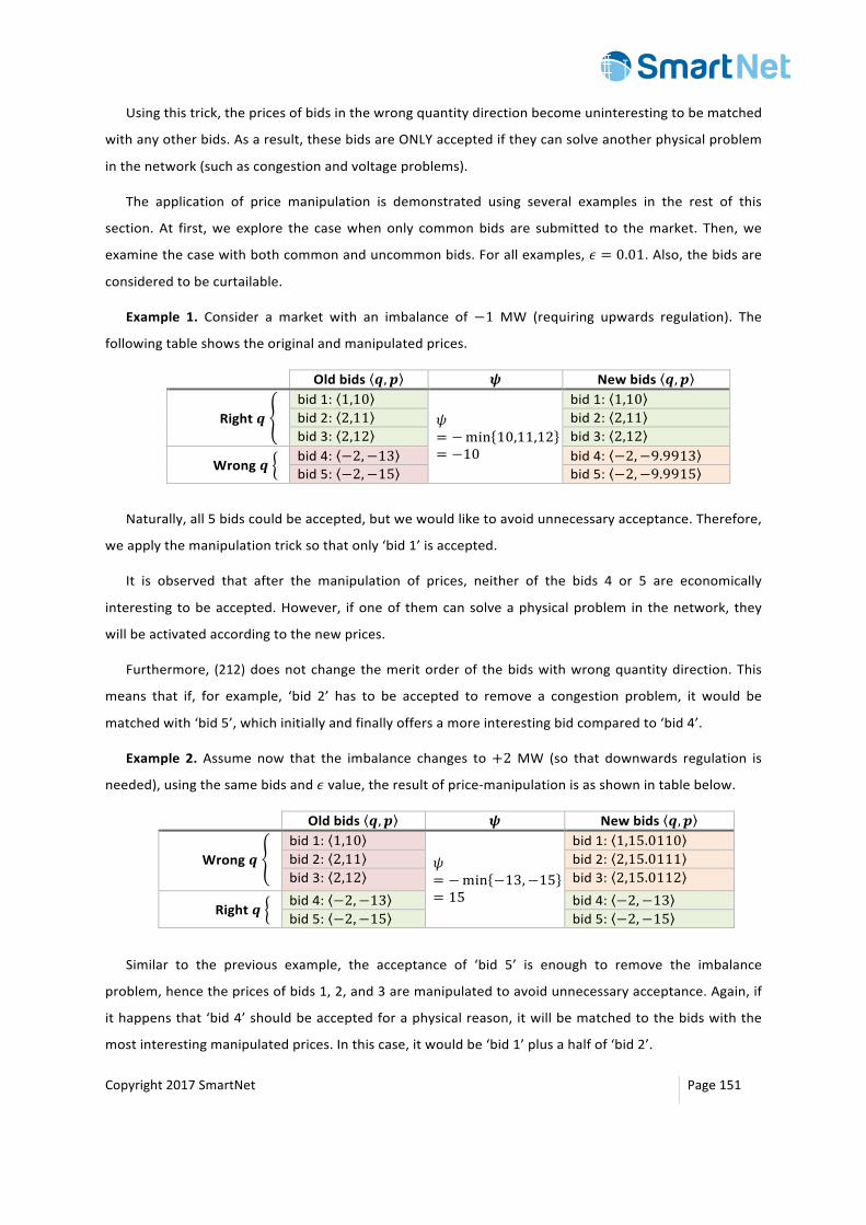
Copyright2017SmartNet Page151
Usingthistrick,thepricesofbidsinthewrongquantitydirectionbecomeuninterestingtobematched
withanyotherbids.Asaresult,thesebidsareONLYacceptediftheycansolveanotherphysicalproblem
inthenetwork(suchascongestionandvoltageproblems).
The application of price manipulation is demonstrated using several examples in the rest of this
section.At first,we explore the casewhenonly commonbids are submitted to themarket. Then,we
examinethecasewithbothcommonanduncommonbids.Forallexamples,𝜖 = 0.01.Also,thebidsare
consideredtobecurtailable.
Example 1. Consider a market with an imbalance of−1 MW (requiring upwards regulation). The
followingtableshowstheoriginalandmanipulatedprices.
Oldbids 𝒒, 𝒑 𝝍 Newbids 𝒒, 𝒑
Right𝒒
bid1: 1,10 𝜓= −min 10,11,12= −10
bid1: 1,10 bid2: 2,11 bid2: 2,11 bid3: 2,12 bid3: 2,12
Wrong𝒒
bid4: −2,−13 bid4: −2,−9.9913 bid5: −2,−15 bid5: −2,−9.9915
Naturally,all5bidscouldbeaccepted,butwewouldliketoavoidunnecessaryacceptance.Therefore,
weapplythemanipulationtricksothatonly‘bid1’isaccepted.
It is observed that after the manipulation of prices, neither of the bids 4 or 5 are economically
interesting tobeaccepted.However, ifoneof themcansolveaphysicalproblem in thenetwork, they
willbeactivatedaccordingtothenewprices.
Furthermore, (212)doesnotchange themeritorderof thebidswithwrongquantitydirection.This
means that if, for example, ‘bid 2’ has to be accepted to remove a congestion problem, it would be
matchedwith‘bid5’,whichinitiallyandfinallyoffersamoreinterestingbidcomparedto‘bid4’.
Example 2. Assume now that the imbalance changes to+2MW (so that downwards regulation is
needed),usingthesamebidsand𝜖value,theresultofprice-manipulationisasshownintablebelow.
Oldbids 𝒒, 𝒑 𝝍 Newbids 𝒒, 𝒑
Wrong𝒒
bid1: 1,10 𝜓= −min −13, −15= 15
bid1: 1,15.0110 bid2: 2,11 bid2: 2,15.0111 bid3: 2,12 bid3: 2,15.0112
Right𝒒
bid4: −2,−13 bid4: −2,−13 bid5: −2,−15 bid5: −2,−15
Similar to the previous example, the acceptance of ‘bid 5’ is enough to remove the imbalance
problem,hencethepricesofbids1,2,and3aremanipulatedtoavoidunnecessaryacceptance.Again,if
ithappensthat‘bid4’shouldbeacceptedforaphysicalreason,itwillbematchedtothebidswiththe
mostinterestingmanipulatedprices.Inthiscase,itwouldbe‘bid1’plusahalfof‘bid2’.
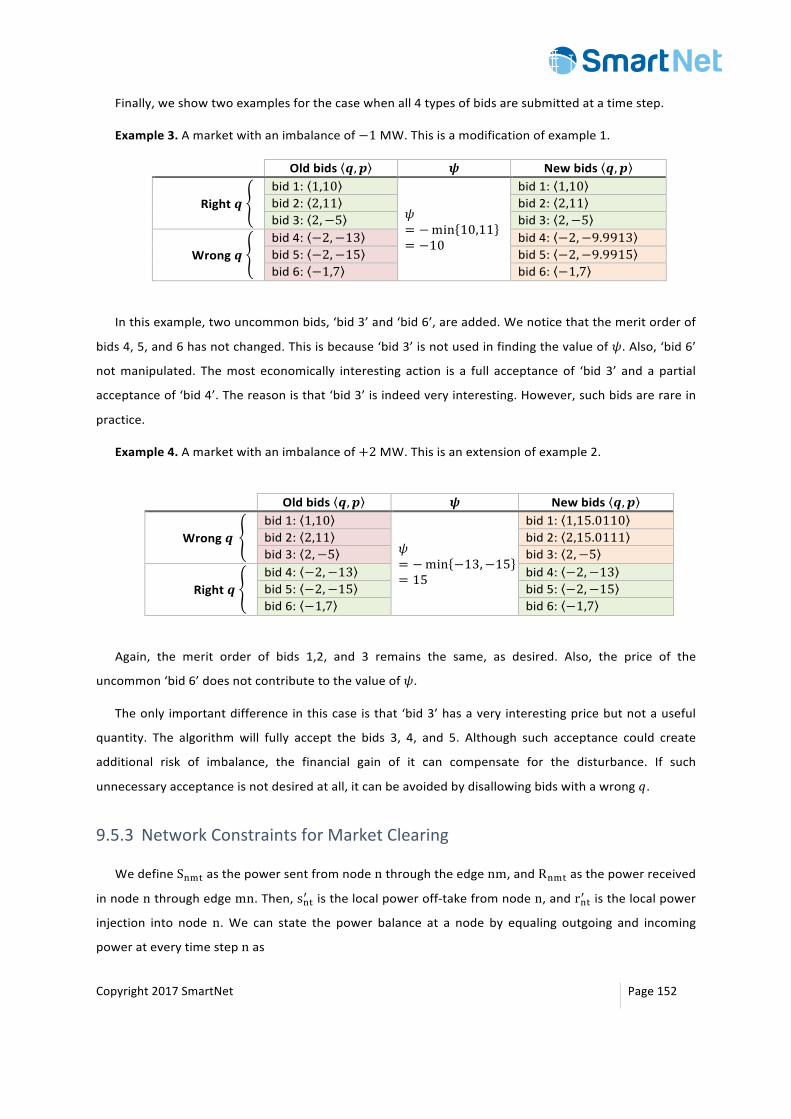
Copyright2017SmartNet Page152
Finally,weshowtwoexamplesforthecasewhenall4typesofbidsaresubmittedatatimestep.
Example3.Amarketwithanimbalanceof−1MW.Thisisamodificationofexample1.
Oldbids 𝒒, 𝒑 𝝍 Newbids 𝒒, 𝒑
Right𝒒
bid1: 1,10
𝜓= −min 10,11= −10
bid1: 1,10 bid2: 2,11 bid2: 2,11 bid3: 2,−5 bid3: 2,−5
Wrong𝒒
bid4: −2,−13 bid4: −2,−9.9913 bid5: −2,−15 bid5: −2,−9.9915 bid6: −1,7 bid6: −1,7
Inthisexample,twouncommonbids,‘bid3’and‘bid6’,areadded.Wenoticethatthemeritorderof
bids4,5,and6hasnotchanged.Thisisbecause‘bid3’isnotusedinfindingthevalueof𝜓.Also,‘bid6’
notmanipulated. Themost economically interesting action is a full acceptanceof ‘bid 3’ and a partial
acceptanceof‘bid4’.Thereasonisthat‘bid3’isindeedveryinteresting.However,suchbidsarerarein
practice.
Example4.Amarketwithanimbalanceof+2MW.Thisisanextensionofexample2.
Oldbids 𝒒, 𝒑 𝝍 Newbids 𝒒, 𝒑
Wrong𝒒
bid1: 1,10
𝜓= −min −13, −15= 15
bid1: 1,15.0110 bid2: 2,11 bid2: 2,15.0111 bid3: 2,−5 bid3: 2,−5
Right𝒒
bid4: −2,−13 bid4: −2,−13 bid5: −2,−15 bid5: −2,−15 bid6: −1,7 bid6: −1,7
Again, the merit order of bids 1,2, and 3 remains the same, as desired. Also, the price of the
uncommon‘bid6’doesnotcontributetothevalueof𝜓.
Theonly importantdifferenceinthiscaseisthat‘bid3’hasaveryinterestingpricebutnotauseful
quantity. The algorithmwill fully accept the bids 3, 4, and 5. Although such acceptance could create
additional risk of imbalance, the financial gain of it can compensate for the disturbance. If such
unnecessaryacceptanceisnotdesiredatall,itcanbeavoidedbydisallowingbidswithawrong𝑞.
9.5.3 NetworkConstraintsforMarketClearing
WedefineSN"Tasthepowersentfromnodenthroughtheedgenm,andRN"Tasthepowerreceived
innodenthroughedgemn.Then,sNTz isthelocalpoweroff-takefromnoden,andrNTz isthelocalpower
injection into noden.We can state the power balance at a node by equaling outgoing and incoming
powerateverytimestepnas
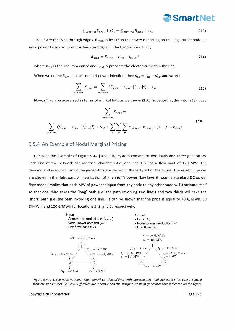
Copyright2017SmartNet Page153
𝑆*(l(:*→( + 𝑠*lz = 𝑅*(l(:(→* + 𝑟*lz (213)
Thepowerreceivedthroughedges,R"NT,islessthanthepowerdepartingontheedgemnatnodem,
sincepowerlossesoccuronthelines(oredges).Infact,morespecifically
𝑅*(l = 𝑆*(l − 𝑧(* ⋅ 𝐼(*lE (214)
wherez"NisthelineimpedanceandI"NTrepresentstheelectriccurrentintheline.
WhenwedefineSN"Tasthelocalnetpowerinjection,thensNT = rNTz − sNTz ,andweget
𝑆*(l(:*→(
= 𝑆*(l − 𝑧(* ⋅ 𝐼(*lE
(:(→*
+ 𝑠*l (215)
Now,sNT" canbeexpressedintermsofmarketbidsaswesawin(210).Substitutingthisinto(215)gives
𝑆*(l(:*→(
=
𝑆(*l − 𝑧(* ⋅ 𝐼(*lE
(:(→*
+ 𝑆*l + 𝑞*+´l� ⋅ 𝑥*+´l� ⋅ (1 + 𝑗 ⋅ 𝑃𝐹*+´)�´+
(216)
9.5.4 AnExampleofNodalMarginalPricing
Consider theexampleof Figure9.44 [109]. The systemconsistsof two loads and threegenerators.
Each line of the network has identical characteristics and line 1-3 has a flow limit of 120 MW. The
demandandmarginalcostofthegeneratorsareshownintheleftpartofthefigure.Theresultingprices
areshownintherightpart.AlinearizationofKirchhoff’spowerflowlawsthroughastandardDCpower
flowmodelimpliesthateachMWofpowershippedfromanynodetoanyothernodewilldistributeitself
so that one third takes the ‘long’ path (i.e. the path involving two lines) and two thirdswill take the
‘short’path (i.e. thepath involvingone line). It canbeshownthat theprice isequal to40€/MWh,80
€/MWh,and120€/MWhforlocations1,2,and3,respectively.
Figure9.44Athree-nodenetwork.Thenetworkconsistsoflineswithidenticalelectricalcharacteristics.Line1-3hasatransmissionlimitof120MW.Off-takesareinelasticandthemarginalcostsofgeneratorsareindicatedonthefigure.
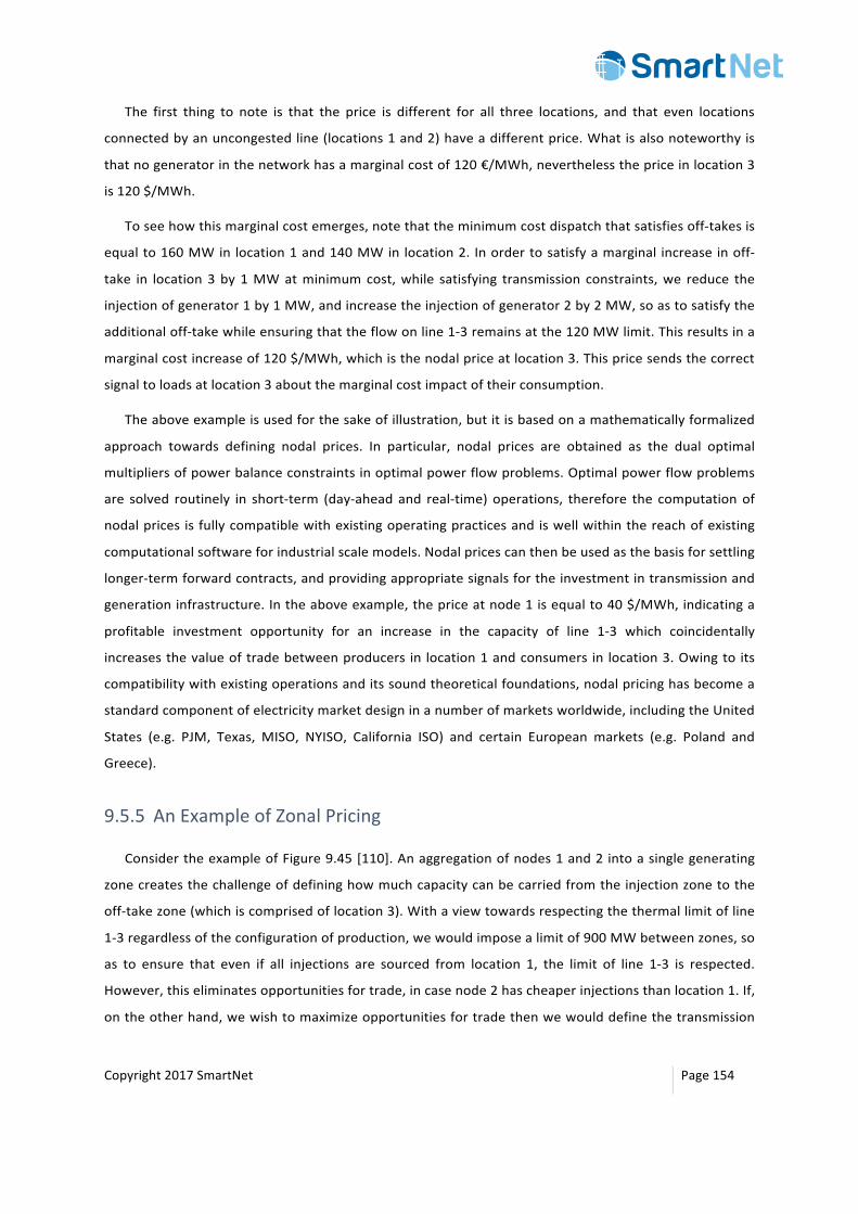
Copyright2017SmartNet Page154
The first thing to note is that the price is different for all three locations, and that even locations
connectedbyanuncongestedline(locations1and2)haveadifferentprice.Whatisalsonoteworthyis
thatnogeneratorinthenetworkhasamarginalcostof120€/MWh,neverthelessthepriceinlocation3
is120$/MWh.
Toseehowthismarginalcostemerges,notethattheminimumcostdispatchthatsatisfiesoff-takesis
equalto160MWinlocation1and140MWinlocation2. Inordertosatisfyamarginal increaseinoff-
take in location3by1MWatminimumcost,while satisfying transmission constraints,we reduce the
injectionofgenerator1by1MW,andincreasetheinjectionofgenerator2by2MW,soastosatisfythe
additionaloff-takewhileensuringthattheflowonline1-3remainsatthe120MWlimit.Thisresultsina
marginalcostincreaseof120$/MWh,whichisthenodalpriceatlocation3.Thispricesendsthecorrect
signaltoloadsatlocation3aboutthemarginalcostimpactoftheirconsumption.
Theaboveexampleisusedforthesakeofillustration,butitisbasedonamathematicallyformalized
approach towards defining nodal prices. In particular, nodal prices are obtained as the dual optimal
multipliersofpowerbalanceconstraintsinoptimalpowerflowproblems.Optimalpowerflowproblems
are solved routinely in short-term (day-aheadand real-time)operations, therefore the computationof
nodalprices isfullycompatiblewithexistingoperatingpracticesandiswellwithinthereachofexisting
computationalsoftwareforindustrialscalemodels.Nodalpricescanthenbeusedasthebasisforsettling
longer-termforwardcontracts,andprovidingappropriatesignalsfortheinvestmentintransmissionand
generationinfrastructure.Intheaboveexample,thepriceatnode1isequalto40$/MWh,indicatinga
profitable investment opportunity for an increase in the capacity of line 1-3 which coincidentally
increasesthevalueoftradebetweenproducers in location1andconsumers in location3.Owingto its
compatibilitywithexistingoperationsanditssoundtheoreticalfoundations,nodalpricinghasbecomea
standardcomponentofelectricitymarketdesigninanumberofmarketsworldwide,includingtheUnited
States (e.g. PJM, Texas, MISO, NYISO, California ISO) and certain European markets (e.g. Poland and
Greece).
9.5.5 AnExampleofZonalPricing
ConsidertheexampleofFigure9.45[110].Anaggregationofnodes1and2intoasinglegenerating
zonecreatesthechallengeofdefininghowmuchcapacitycanbecarriedfromtheinjectionzonetothe
off-takezone(whichiscomprisedoflocation3).Withaviewtowardsrespectingthethermallimitofline
1-3regardlessoftheconfigurationofproduction,wewouldimposealimitof900MWbetweenzones,so
as to ensure that even if all injections are sourced from location 1, the limit of line 1-3 is respected.
However,thiseliminatesopportunitiesfortrade,incasenode2hascheaperinjectionsthanlocation1.If,
ontheotherhand,wewishtomaximizeopportunitiesfortradethenwewoulddefinethetransmission
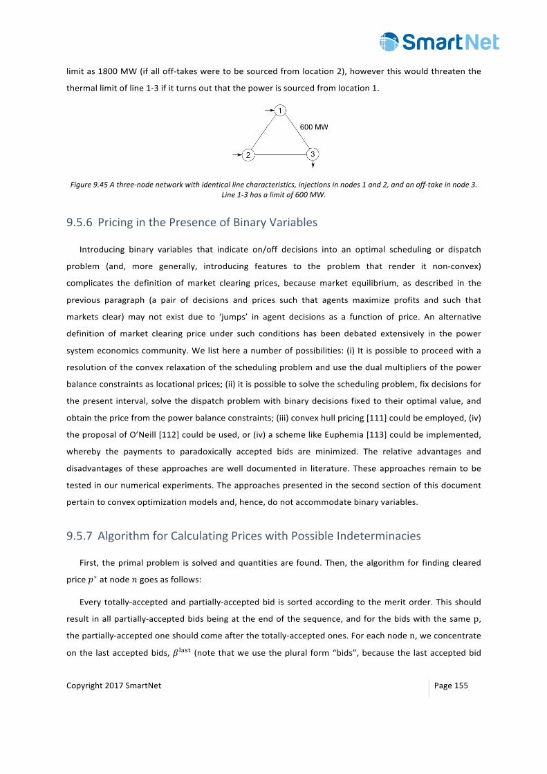
Copyright2017SmartNet Page155
limitas1800MW(ifalloff-takesweretobesourcedfromlocation2),howeverthiswouldthreatenthe
thermallimitofline1-3ifitturnsoutthatthepowerissourcedfromlocation1.
Figure9.45Athree-nodenetworkwithidenticallinecharacteristics,injectionsinnodes1and2,andanoff-takeinnode3.Line1-3hasalimitof600MW.
9.5.6 PricinginthePresenceofBinaryVariables
Introducing binary variables that indicate on/off decisions into an optimal scheduling or dispatch
problem (and, more generally, introducing features to the problem that render it non-convex)
complicates the definition of market clearing prices, because market equilibrium, as described in the
previous paragraph (a pair of decisions and prices such that agents maximize profits and such that
markets clear) may not exist due to ‘jumps’ in agent decisions as a function of price. An alternative
definition of market clearing price under such conditions has been debated extensively in the power
systemeconomicscommunity.Welisthereanumberofpossibilities:(i) It ispossibletoproceedwitha
resolutionoftheconvexrelaxationoftheschedulingproblemandusethedualmultipliersofthepower
balanceconstraintsaslocationalprices;(ii)itispossibletosolvetheschedulingproblem,fixdecisionsfor
thepresent interval, solve thedispatchproblemwithbinarydecisions fixedto theiroptimalvalue,and
obtainthepricefromthepowerbalanceconstraints;(iii)convexhullpricing[111]couldbeemployed,(iv)
theproposalofO’Neill[112]couldbeused,or(iv)aschemelikeEuphemia[113]couldbeimplemented,
whereby the payments to paradoxically accepted bids are minimized. The relative advantages and
disadvantagesof these approaches arewell documented in literature. These approaches remain tobe
testedinournumericalexperiments.Theapproachespresentedinthesecondsectionofthisdocument
pertaintoconvexoptimizationmodelsand,hence,donotaccommodatebinaryvariables.
9.5.7 AlgorithmforCalculatingPriceswithPossibleIndeterminacies
First, theprimalproblem issolvedandquantitiesare found.Then, thealgorithmfor findingcleared
price𝑝∗atnode𝑛goesasfollows:
Every totally-acceptedandpartially-acceptedbid issortedaccordingto themeritorder.Thisshould
result inallpartially-acceptedbidsbeingattheendofthesequence,andforthebidswiththesamep,
thepartially-acceptedoneshouldcomeafterthetotally-acceptedones.Foreachnoden,weconcentrate
onthe lastacceptedbids,𝛽jO6T (notethatweusetheplural form“bids”,becausethe lastacceptedbid
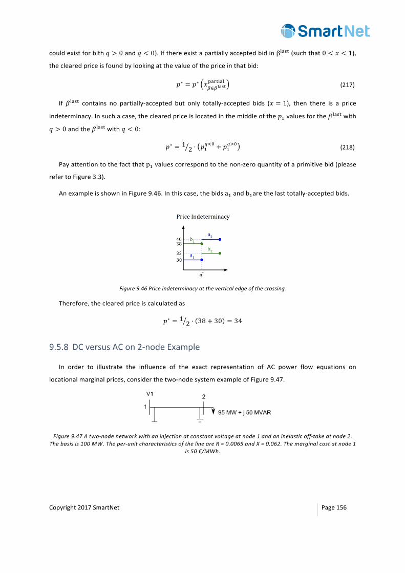
Copyright2017SmartNet Page156
couldexistforbith𝑞 > 0and𝑞 < 0).IfthereexistapartiallyacceptedbidinβjO6T(suchthat0 < 𝑥 < 1),
theclearedpriceisfoundbylookingatthevalueofthepriceinthatbid:
𝑝∗ = 𝑝∗ 𝑥�∈�klmnoOpTHOj (217)
If𝛽jO6T contains no partially-accepted but only totally-accepted bids (𝑥 = 1), then there is a price
indeterminacy.Insuchacase,theclearedpriceislocatedinthemiddleofthe𝑝4valuesforthe𝛽jO6Twith
𝑞 > 0andthe𝛽jO6Twith𝑞 < 0:
𝑝∗ = 12 ⋅ 𝑝4
qr3 + 𝑝4qs3 (218)
Payattentiontothefactthatp4valuescorrespondtothenon-zeroquantityofaprimitivebid(please
refertoFigure3.3).
AnexampleisshowninFigure9.46.Inthiscase,thebidsa4andb4arethelasttotally-acceptedbids.
Figure9.46Priceindeterminacyattheverticaledgeofthecrossing.
Therefore,theclearedpriceiscalculatedas
𝑝∗ = 12 ⋅ 38 + 30 = 34
9.5.8 DCversusACon2-nodeExample
In order to illustrate the influence of the exact representation of AC power flow equations on
locationalmarginalprices,considerthetwo-nodesystemexampleofFigure9.47.
Figure9.47Atwo-nodenetworkwithaninjectionatconstantvoltageatnode1andaninelasticoff-takeatnode2.Thebasisis100MW.Theper-unitcharacteristicsofthelineareR=0.0065andX=0.062.Themarginalcostatnode1
is50€/MWh.
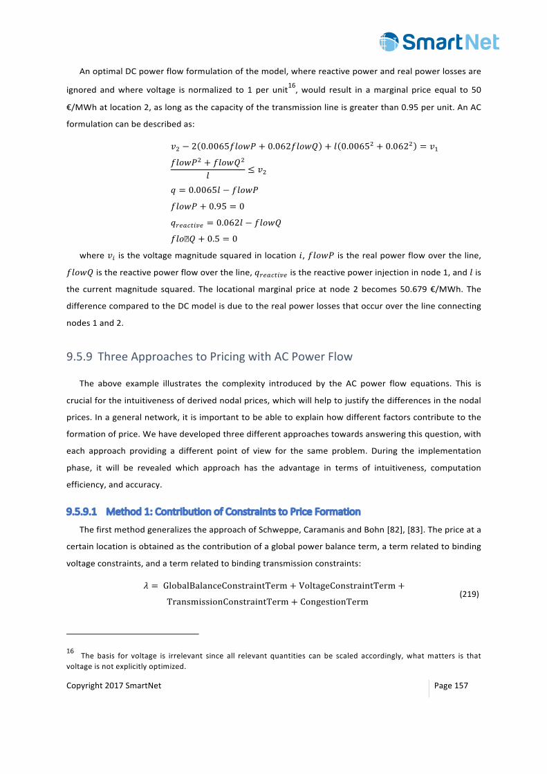
Copyright2017SmartNet Page157
AnoptimalDCpowerflowformulationofthemodel,wherereactivepowerandrealpowerlossesare
ignored andwhere voltage is normalized to 1 per unit16,would result in amarginal price equal to 50
€/MWhatlocation2,aslongasthecapacityofthetransmissionlineisgreaterthan0.95perunit.AnAC
formulationcanbedescribedas:
𝑣E − 2 0.0065𝑓𝑙𝑜𝑤𝑃 + 0.062𝑓𝑙𝑜𝑤𝑄 + 𝑙 0.0065E + 0.062E = 𝑣4
𝑓𝑙𝑜𝑤𝑃E + 𝑓𝑙𝑜𝑤𝑄E
𝑙≤ 𝑣E
𝑞 = 0.0065𝑙 − 𝑓𝑙𝑜𝑤𝑃
𝑓𝑙𝑜𝑤𝑃 + 0.95 = 0
𝑞km+�l)'m = 0.062𝑙 − 𝑓𝑙𝑜𝑤𝑄
𝑓𝑙𝑜�𝑄 + 0.5 = 0
where𝑣) isthevoltagemagnitudesquaredinlocation𝑖,𝑓𝑙𝑜𝑤𝑃 istherealpowerflowovertheline,
𝑓𝑙𝑜𝑤𝑄isthereactivepowerflowovertheline,𝑞km+�l)'m isthereactivepowerinjectioninnode1,and𝑙is
the currentmagnitude squared. The locationalmarginal price at node2becomes50.679€/MWh. The
differencecomparedtotheDCmodelisduetotherealpowerlossesthatoccuroverthelineconnecting
nodes1and2.
9.5.9 ThreeApproachestoPricingwithACPowerFlow
The above example illustrates the complexity introduced by the AC power flow equations. This is
crucialfortheintuitivenessofderivednodalprices,whichwillhelptojustifythedifferencesinthenodal
prices.Inageneralnetwork,itisimportanttobeabletoexplainhowdifferentfactorscontributetothe
formationofprice.Wehavedevelopedthreedifferentapproachestowardsansweringthisquestion,with
each approach providing a different point of view for the same problem. During the implementation
phase, it will be revealed which approach has the advantage in terms of intuitiveness, computation
efficiency,andaccuracy.
9.5.9.1 Method1:ContributionofConstraintstoPriceFormation
ThefirstmethodgeneralizestheapproachofSchweppe,CaramanisandBohn[82],[83].Thepriceata
certainlocationisobtainedasthecontributionofaglobalpowerbalanceterm,atermrelatedtobinding
voltageconstraints,andatermrelatedtobindingtransmissionconstraints:
𝜆 = GlobalBalanceConstraintTerm + VoltageConstraintTerm +
TransmissionConstraintTerm + CongestionTerm(219)
16 The basis for voltage is irrelevant since all relevant quantities can be scaled accordingly,whatmatters is thatvoltageisnotexplicitlyoptimized.
Copyright2017SmartNet Page158
Eachofthefourtermsabovedependonnetworkparameters(forexample,impedanceandreactance
oflines)andthepartialderivativeofthedecisionvariableswithrespecttoanetinjectionofrealpowerin
thenodewhosepricewearecomputing.Thispartialderivativebecomesanalyticallycomplextoderive
evenforthesimpletwo-nodenetworkofFigure9.47,andispracticallyimpossibletoderiveanalytically
for a network with arbitrary topology. Therefore, each of these terms needs to be approximated
numerically by re-solving theoptimalpower flowproblemwith a slightperturbation in theamountof
powerinjectioninthenodewhosepricewearecomputing.
Thekeytotheaboveresultistouseawell-knownresultinpowersystemanalysis:allpowerflowscan
bedescribedasafunctionoftherootnodevoltagemagnitude,andrealandreactivepowerinjectionsat
thenodes.Inintuitiveterms,thismeansthatifweweretoldthevoltagemagnitudeattherootandthe
real and reactivepower injections at all locationsof thenetwork thenwe coulddetermine thepower
flows over the entire network.We can thenwrite out the optimization problem in terms of the root
voltagemagnitude,realinjectionsandreactiveinjections.Relaxingthevoltageconstraints,transmission
constraints,andglobalpowerbalanceconstraintoftheproblemyieldsaLagrangianfunction,whosefirst-
orderconditionswithrespecttorealpowerinjectioncanbeusedtoderivetherelationshipabove.
9.5.9.2 Method2:ContributionofLossestoPriceFormation
Thestartingpointofthesecondmethodisthesensitivityinterpretationofprices:therealpowerprice
ofacertainlocationisthesensitivityofcosttoamarginalchangeinrealpowerinjectionsinthatsame
location.Sincecostcanbeexpressedasafunctionoftotalrealpower,whichinturncanbeexpressedas
thesumofrealpowerconsumptionpluslossesintheentirenetwork,weobtainthefollowing:
𝜆 ≃ 𝜆((1 +n<Âttmt8n|É)∈} ) (220)
whereλ" is themarginal cost of themarginal generator,E is the set of lines of the network, and��b66d6����
is the total derivativeof the real power losseswith respect to real power consumption in the
locationwhosepricewearecomputing.Themarginalgeneratoristhegeneratorthatisproducingstrictly
above its technical minimum and strictly below its technical maximum, and whose output would be
expected tochange inorder tosatisfyachange in the realpowerconsumption for the locationwhose
pricewearecomputing.Asinthecaseofthepreviousmethod,thefullderivativescannotbecomputed
analyticallyandneedtobeapproximatednumerically.
Itisworthnotingthattherelationaboveisnotexact,sinceitdoesnotaccountforthesecond-order
effectthatnon-marginalgeneratorrealpoweradjustmentshaveontheobjectivefunction.Nevertheless,
experimentalexperienceonaCIGRE15-busnetworkshowthatitpredictspriceswithanaccuracywhich
isnoworsethan0.1€/MWh.Additionaltestsonnetworksofdifferentsizesandtopologieswouldhaveto
beperformedinordertoverifytheprecisionoftheaboveformula.
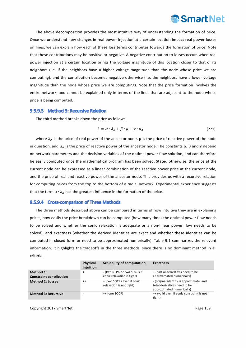
Copyright2017SmartNet Page159
Theabovedecompositionprovides themost intuitivewayofunderstanding the formationofprice.
Onceweunderstandhowchangesinrealpowerinjectionatacertainlocationimpactrealpowerlosses
onlines,wecanexplainhoweachoftheselosstermscontributestowardstheformationofprice.Note
thatthesecontributionsmaybepositiveornegative.Anegativecontributiontolossesoccurswhenreal
power injection at a certain locationbrings the voltagemagnitudeof this location closer to thatof its
neighbors (i.e. if the neighbors have a higher voltage magnitude than the node whose price we are
computing),and thecontributionbecomesnegativeotherwise (i.e. theneighborshavea lowervoltage
magnitude than the nodewhose pricewe are computing).Note that the price formation involves the
entirenetwork,andcannotbeexplainedonlyintermsofthelinesthatareadjacenttothenodewhose
priceisbeingcomputed.
9.5.9.3 Method3:RecursiveRelation
Thethirdmethodbreaksdownthepriceasfollows:
𝜆 = 𝛼 ∙ 𝜆� + 𝛽 ∙ 𝜇 + 𝛾 ∙ 𝜇� (221)
whereλ�isthepriceofrealpoweroftheancestornode,µisthepriceofreactivepowerofthenode
inquestion,andµ�isthepriceofreactivepoweroftheancestornode.Theconstantsα,βandγdepend
onnetworkparametersandthedecisionvariablesoftheoptimalpowerflowsolution,andcantherefore
beeasilycomputedoncethemathematicalprogramhasbeensolved.Statedotherwise,thepriceatthe
currentnodecanbeexpressedasalinearcombinationofthereactivepowerpriceatthecurrentnode,
andthepriceofrealandreactivepoweroftheancestornode.Thisprovidesuswitharecursiverelation
forcomputingpricesfromthetoptothebottomofaradialnetwork.Experimentalexperiencesuggests
thatthetermα ∙ λ�hasthegreatestinfluenceintheformationoftheprice.
9.5.9.4 Cross-comparisonofThreeMethods
Thethreemethodsdescribedabovecanbecomparedintermsofhowintuitivetheyareinexplaining
prices,howeasilythepricebreakdowncanbecomputed(howmanytimestheoptimalpowerflowneeds
to be solved and whether the conic relaxation is adequate or a non-linear power flow needs to be
solved), and exactness (whether the derived identities are exact and whether these identities can be
computed inclosed formorneed tobeapproximatednumerically).Table9.1 summarizes the relevant
information. Ithighlights the tradeoffs in the threemethods, since there isnodominantmethod inall
criteria.
Physicalintuition
Scalabilityofcomputation Exactness
Method1:Constraintcontribution
+ -(twoNLPs,ortwoSOCPsifconicrelaxationistight)
+(partialderivativesneedtobeapproximatednumerically)
Method2:Losses ++ +(twoSOCPsevenifconicrelaxationisnottight)
-(originalidentityisapproximate,andtotalderivativesneedtobeapproximatednumerically)
Method3:Recursive - ++(oneSOCP) ++(validevenifconicconstraintisnottight)

Copyright2017SmartNet Page160
Table9.1Comparisonofthreemethods.
Ourrecommendationforthepreferableapproachismethod2,basedonlosses,sinceitisthemethod
bestgroundedonphysical intuition,whilebeingacceptablyaccurateandscalable(itrequirestwicethe
amountofcomputationcomparedtomethod3,andreliesontheresolutionofanSOCPrelaxationwithin
an operationally acceptable timeframe, which is a working assumption of the SmartNet project). The
accuracy of the method has been verified through experiments: for the CIGRE 15-node model the
methodpredictspriceswithanaccuracyof0.1€/MWh.