Session 5: Nominal Rigidities

Jean Imbs

December 2010

Imbs Rigidities

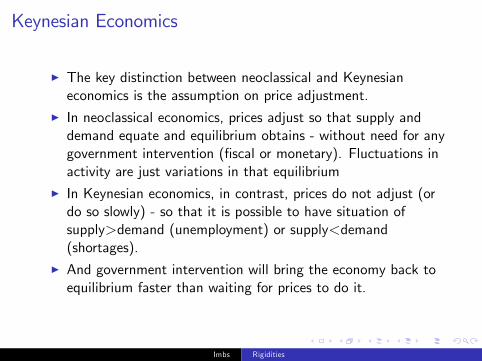
Keynesian Economics

I The key distinction between neoclassical and Keynesianeconomics is the assumption on price adjustment.

I In neoclassical economics, prices adjust so that supply anddemand equate and equilibrium obtains - without need for anygovernment intervention (�scal or monetary). Fluctuations inactivity are just variations in that equilibrium

I In Keynesian economics, in contrast, prices do not adjust (ordo so slowly) - so that it is possible to have situation ofsupply>demand (unemployment) or supply<demand(shortages).

I And government intervention will bring the economy back toequilibrium faster than waiting for prices to do it.

Imbs Rigidities

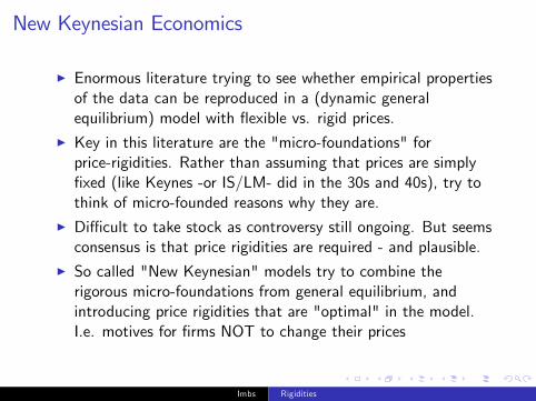
New Keynesian Economics

I Enormous literature trying to see whether empirical propertiesof the data can be reproduced in a (dynamic generalequilibrium) model with �exible vs. rigid prices.

I Key in this literature are the "micro-foundations" forprice-rigidities. Rather than assuming that prices are simply�xed (like Keynes -or IS/LM- did in the 30s and 40s), try tothink of micro-founded reasons why they are.

I Di¢ cult to take stock as controversy still ongoing. But seemsconsensus is that price rigidities are required - and plausible.

I So called "New Keynesian" models try to combine therigorous micro-foundations from general equilibrium, andintroducing price rigidities that are "optimal" in the model.I.e. motives for �rms NOT to change their prices

Imbs Rigidities

Mircro-foundations of Price Rigidities

I Three ingredientsI Firms are STILL optimizingI There is imperfect competition (either in goods or in labormarkets), so that �rms are price-SETTERS.

I And thus can choose optimally potentially NOT to adjustprices. Or to adjust them slowly. In perfect competition,prices are GIVEN by the market!

Imbs Rigidities

Consequences

I So now individual �rms may choose to change their pricesluggishly. First, this requires a model of individual pricesetting, for individual goods (as opposed to a model of theoverall price level - i.e. of CPI)

I Second this has implications on the sluggishness of in�ation asa whole - which may become more sticky as a result

I So we need a framework with monopolistic competition, eitherin goods or in labor markets.

Imbs Rigidities

Monopolistic Competition

I Under perfect competition, prices are equal to marginal costs,since otherwise they are competed down.To be able to setprices, �rms must have a degree of monopoly power, i.e.something that prevents the consumers from bidding the pricedown.

I With monopoly power on the goods market, �rms can chargeprices at a markup over the marginal cost. (Same withmonopoly power on the labor market -either on employer oremployee side- resulting in wages di¤erent from the MPL)

I The conventional theory is one of "monopolistic competition",where there is a large range of di¤erent goods and services,each one being imperfect substitute for the others, and eachone being produced by a �rm.

I That �rm therefore exerts some monopoly power over its ownvariety

Imbs Rigidities

Monopolistic Competition - Firms

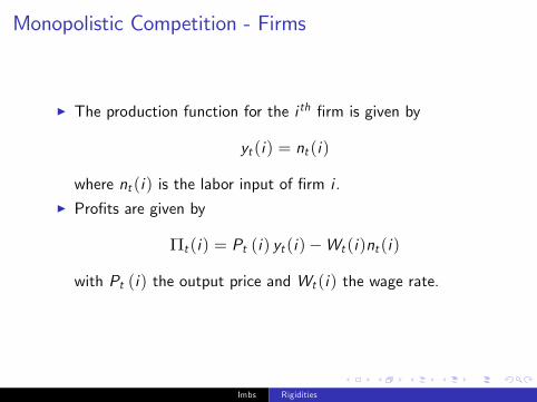
I The production function for the i th �rm is given by

yt (i) = nt (i)

where nt (i) is the labor input of �rm i .I Pro�ts are given by

Πt (i) = Pt (i) yt (i)�Wt (i)nt (i)

with Pt (i) the output price and Wt (i) the wage rate.

Imbs Rigidities

Monopolistic Competition - Households

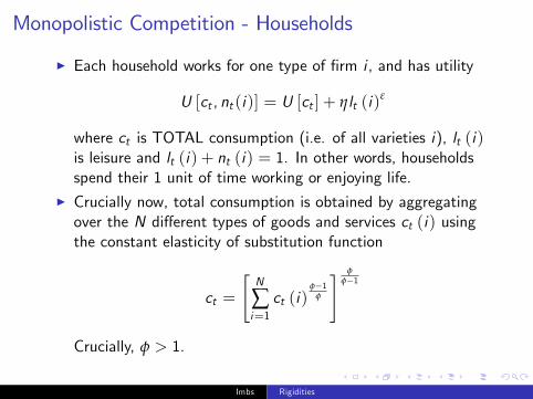
I Each household works for one type of �rm i , and has utility

U [ct , nt (i)] = U [ct ] + ηlt (i)ε

where ct is TOTAL consumption (i.e. of all varieties i), lt (i)is leisure and lt (i) + nt (i) = 1. In other words, householdsspend their 1 unit of time working or enjoying life.

I Crucially now, total consumption is obtained by aggregatingover the N di¤erent types of goods and services ct (i) usingthe constant elasticity of substitution function

ct =

"N

∑i=1ct (i)

φ�1φ

# φφ�1

Crucially, φ > 1.

Imbs Rigidities

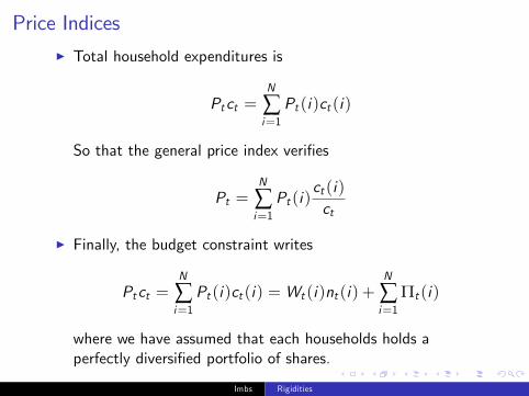
Price IndicesI Total household expenditures is

Ptct =N

∑i=1Pt (i)ct (i)

So that the general price index veri�es

Pt =N

∑i=1Pt (i)

ct (i)ct

I Finally, the budget constraint writes

Ptct =N

∑i=1Pt (i)ct (i) = Wt (i)nt (i) +

N

∑i=1

Πt (i)

where we have assumed that each households holds aperfectly diversi�ed portfolio of shares.

Imbs Rigidities

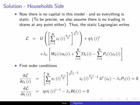
Solution - Households SideI Now there is no capital in this model - and so everything isstatic. (To be precise, we also assume there is no trading inshares at any point either). Thus, the static Lagrangian writes

L = U

0@" N

∑i=1ct (i)

φ�1φ

# φφ�11A+ ηlt (i)

ε

+λt

"Wt (i)nt (i) +

N

∑i=1

Πt (i)�N

∑i=1Pt (i)ct (i)

#I First order conditions

∂L∂ct (i)

=

"N

∑i=1ct (i)

φ�1φ

# φφ�1�1

ct (i)φ�1

φ �1 U 0 (ct )� λtPt (i) = 0

∂L∂lt (i)

= ηεlt (i)ε�1 � λtWt (i) = 0

Imbs Rigidities

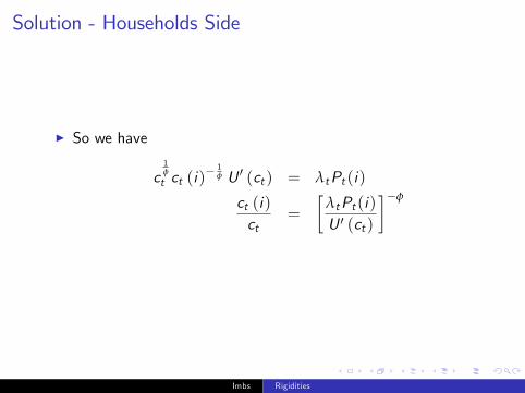
Solution - Households Side

I So we have

c1φ

t ct (i)� 1

φ U 0 (ct ) = λtPt (i)

ct (i)ct

=

�λtPt (i)U 0 (ct )

��φ

Imbs Rigidities

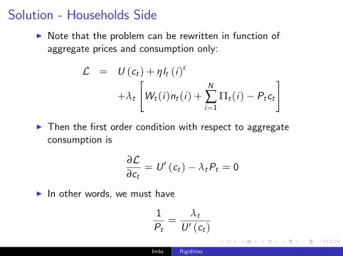
Solution - Households SideI Note that the problem can be rewritten in function ofaggregate prices and consumption only:

L = U (ct ) + ηlt (i)ε

+λt

"Wt (i)nt (i) +

N

∑i=1

Πt (i)� Ptct

#I Then the �rst order condition with respect to aggregateconsumption is

∂L∂ct

= U 0 (ct )� λtPt = 0

I In other words, we must have

1Pt=

λtU 0 (ct )

Imbs Rigidities

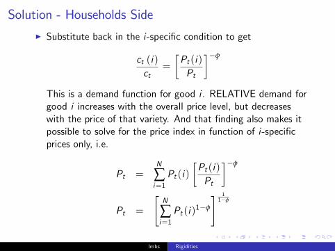
Solution - Households Side

I Substitute back in the i-speci�c condition to get

ct (i)ct

=

�Pt (i)Pt

��φ

This is a demand function for good i . RELATIVE demand forgood i increases with the overall price level, but decreaseswith the price of that variety. And that �nding also makes itpossible to solve for the price index in function of i-speci�cprices only, i.e.

Pt =N

∑i=1Pt (i)

�Pt (i)Pt

��φ

Pt =

"N

∑i=1Pt (i)1�φ

# 11�φ

Imbs Rigidities

Solution - Households Side

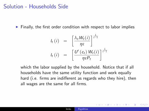
I Finally, the �rst order condition with respect to labor implies

lt (i) =

�λtWt (i)

ηε

� 1ε�1

lt (i) =

�U 0 (ct )Wt (i)

ηεPt

� 1ε�1

which the labor supplied by the household. Notice that if allhouseholds have the same utility function and work equallyhard (i.e. �rms are indi¤erent as regards who they hire), thenall wages are the same for all �rms.

Imbs Rigidities

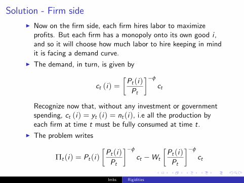
Solution - Firm sideI Now on the �rm side, each �rm hires labor to maximizepro�ts. But each �rm has a monopoly onto its own good i ,and so it will choose how much labor to hire keeping in mindit is facing a demand curve.

I The demand, in turn, is given by

ct (i) =�Pt (i)Pt

��φ

ct

Recognize now that, without any investment or governmentspending, ct (i) = yt (i) = nt (i), i.e all the production byeach �rm at time t must be fully consumed at time t.

I The problem writes

Πt (i) = Pt (i)�Pt (i)Pt

��φ

ct �Wt

�Pt (i)Pt

��φ

ct

Imbs Rigidities

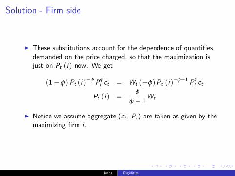
Solution - Firm side

I These substitutions account for the dependence of quantitiesdemanded on the price charged, so that the maximization isjust on Pt (i) now. We get

(1� φ)Pt (i)�φ Pφ

t ct = Wt (�φ)Pt (i)�φ�1 Pφ

t ct

Pt (i) =φ

φ� 1Wt

I Notice we assume aggregate (ct , Pt) are taken as given by themaximizing �rm i .

Imbs Rigidities

Solution - Firm side

I This is the central result of monopolistic competition. FirmsCHOOSE a price at a markup φ

φ�1 > 1 over marginal costs,which here are just wages (since production is linear in labor).Prices vary across goods because of (potential) di¤erences inthe marginal cost. The point is, �rms have some control overtheir prices.

I Notice that when φ ! ∞, the markup tends to unity. Makessense since φ ! ∞ means goods become perfect substitutes,i.e. competition becomes perfect. In other words, theelasticity of substitution φ captures precisely the extent ofcompetition, in that it maps directly with �rms�pro�tsmargins (which end up identical across �rms in equilibrium)

Imbs Rigidities

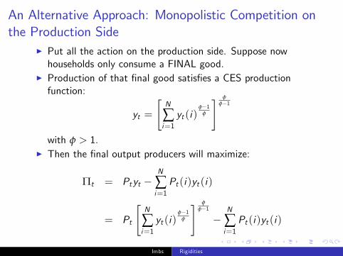
An Alternative Approach: Monopolistic Competition onthe Production Side

I Put all the action on the production side. Suppose nowhouseholds only consume a FINAL good.

I Production of that �nal good satis�es a CES productionfunction:

yt =

"N

∑i=1yt (i)

φ�1φ

# φφ�1

with φ > 1.I Then the �nal output producers will maximize:

Πt = Ptyt �N

∑i=1Pt (i)yt (i)

= Pt

"N

∑i=1yt (i)

φ�1φ

# φφ�1

�N

∑i=1Pt (i)yt (i)

Imbs Rigidities

An Alternative Approach: Monopolistic Competition onthe Production Side

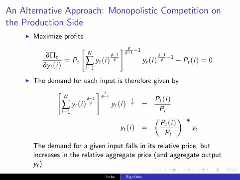
I Maximize pro�ts

∂Πt

∂yt (i)= Pt

"N

∑i=1yt (i)

φ�1φ

# φφ�1�1

yt (i)φ�1

φ �1 � Pt (i) = 0

I The demand for each input is therefore given by"N

∑i=1yt (i)

φ�1φ

# 1φ�1

yt (i)� 1

φ =Pt (i)Pt

yt (i) =

�Pt (i)Pt

��φ

yt

The demand for a given input falls in its relative price, butincreases in the relative aggregate price (and aggregate outputyt)

Imbs Rigidities

An Alternative Approach: Monopolistic Competition onthe Production Side

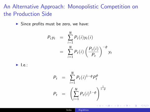
I Since pro�ts must be zero, we have:

Ptyt =N

∑i=1Pt (i)yt (i)

=N

∑i=1Pt (i)

�Pt (i)Pt

��φ

yt

I I.e.:

Pt =N

∑i=1Pt (i)1�φPφ

t

Pt =

N

∑i=1Pt (i)1�φ

! 11�φ

Imbs Rigidities

An Alternative Approach: Monopolistic Competition onthe Production Side

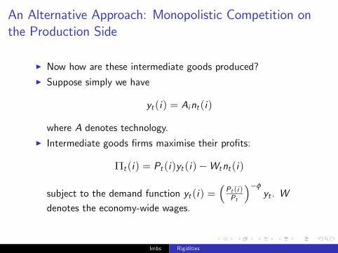
I Now how are these intermediate goods produced?I Suppose simply we have

yt (i) = Aint (i)

where A denotes technology.I Intermediate goods �rms maximise their pro�ts:

Πt (i) = Pt (i)yt (i)�Wtnt (i)

subject to the demand function yt (i) =�Pt (i )Pt

��φyt . W

denotes the economy-wide wages.

Imbs Rigidities

An Alternative Approach: Monopolistic Competition onthe Production Side

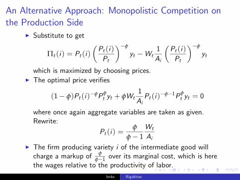
I Substitute to get

Πt (i) = Pt (i)�Pt (i)Pt

��φ

yt �Wt1Ai

�Pt (i)Pt

��φ

yt

which is maximized by choosing prices.I The optimal price veri�es

(1� φ)Pt (i)�φPφt yt + φWt

1AiPt (i)�φ�1Pφ

t yt = 0

where once again aggregate variables are taken as given.Rewrite:

Pt (i) =φ

φ� 1Wt

AiI The �rm producing variety i of the intermediate good willcharge a markup of φ

φ�1 over its marginal cost, which is herethe wages relative to the productivity of labor.

Imbs Rigidities

Sources of Nominal Rigidities

I Now we have established a way to think about price-settingdecisions on the part of �rms.

I How does that translate in AGGREGATE price dynamics?I Two approaches:

I Taylor model of overlapping contractsI Calvo model of staggered price adjustment

Imbs Rigidities

Taylor "staggered" contracts

I Price is a markup over marginal costs, and the markup maybe time varying.

I At any point in time, the wage rate is an average of wagecontracts that were set in the past, but are still in force, andthose set in the current period.

I AT THE TIME THEY WERE SET, wage contracts werepro�t maximizing, and re�ected the prevailing MPL and theexpected future price level.

Imbs Rigidities

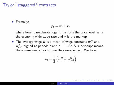
Taylor "staggered" contracts

I Formally:pt = wt + vt

where lower case denote logarithms, p is the price level, w isthe economy-wide wage rate and v is the markup

I The average wage w is a mean of wage contracts wNt andwNt�1 signed at periods t and t � 1. An N superscript meansthese were new at each time they were signed. We have

wt =12

�wNt + w

Nt�1

�

Imbs Rigidities

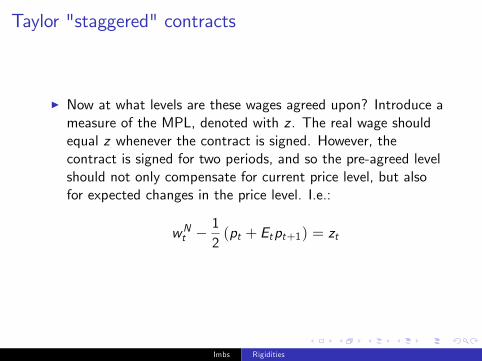
Taylor "staggered" contracts

I Now at what levels are these wages agreed upon? Introduce ameasure of the MPL, denoted with z . The real wage shouldequal z whenever the contract is signed. However, thecontract is signed for two periods, and so the pre-agreed levelshould not only compensate for current price level, but alsofor expected changes in the price level. I.e.:

wNt �12(pt + Etpt+1) = zt

Imbs Rigidities

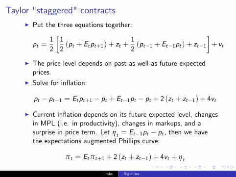
Taylor "staggered" contractsI Put the three equations together:

pt =12

�12(pt + Etpt+1) + zt +

12(pt�1 + Et�1pt ) + zt�1

�+ vt

I The price level depends on past as well as future expectedprices.

I Solve for in�ation:

pt � pt�1 = Etpt+1 � pt + Et�1pt � pt + 2 (zt + zt�1) + 4vt

I Current in�ation depends on its future expected level, changesin MPL (i.e. in productivity), changes in markups, and asurprise in price term. Let ηt = Et�1pt � pt , then we havethe expectations augmented Phillips curve:

πt = Etπt+1 + 2 (zt + zt�1) + 4vt + ηt

Imbs Rigidities

Calvo "staggered"price adjustment

I Aggregate price dynamics here the outcome of individual �rmsdecisions. Still, framework very tractable - reason whyprobably the most popular approach.

I Firms are forward looking, and they forecast the optimal pricep�t+s . They all have the same forecast, but not all are allowedto change their prices. In particular, each period, there is aprobability ρ that a �rm will be able to adjust its price to theoptimum.

I In other words, �rms have no control about when they canadjust their price - although they do it optimally when theycan.

Imbs Rigidities

Calvo "staggered"price adjustment

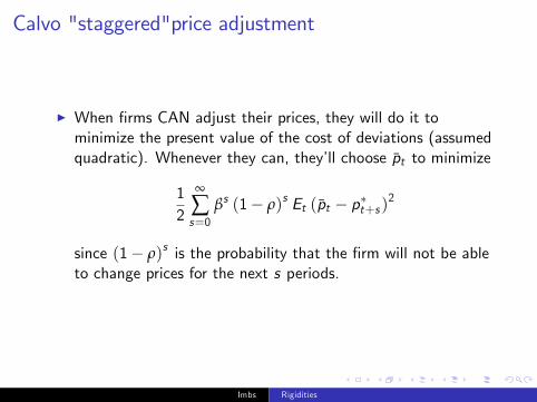
I When �rms CAN adjust their prices, they will do it tominimize the present value of the cost of deviations (assumedquadratic). Whenever they can, they�ll choose p̄t to minimize

12

∞

∑s=0

βs (1� ρ)s Et (p̄t � p�t+s )2

since (1� ρ)s is the probability that the �rm will not be ableto change prices for the next s periods.

Imbs Rigidities

Calvo "staggered"price adjustment

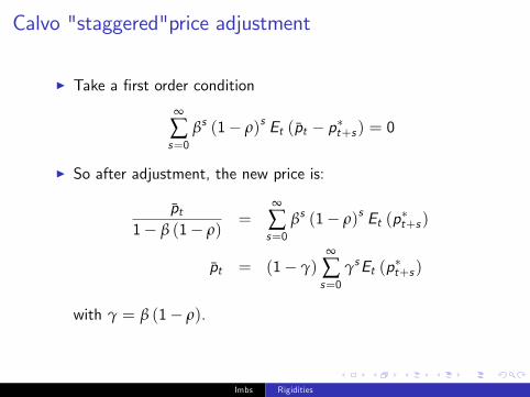
I Take a �rst order condition

∞

∑s=0

βs (1� ρ)s Et (p̄t � p�t+s ) = 0

I So after adjustment, the new price is:

p̄t1� β (1� ρ)

=∞

∑s=0

βs (1� ρ)s Et (p�t+s )

p̄t = (1� γ)∞

∑s=0

γsEt (p�t+s )

with γ = β (1� ρ).

Imbs Rigidities

Calvo "staggered"price adjustment

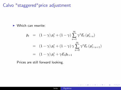
I Which can rewrite:

p̄t = (1� γ) p�t + (1� γ)∞

∑s=1

γsEt (p�t+s )

= (1� γ) p�t + (1� γ) γ∞

∑s=0

γsEt (p�t+s+1)

= (1� γ) p�t + γEt p̄t+1

Prices are still forward looking.

Imbs Rigidities

Calvo "staggered"price adjustment

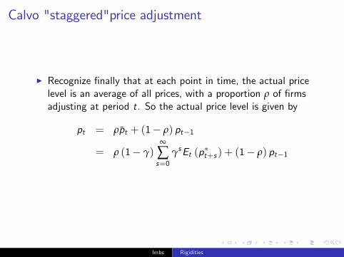
I Recognize �nally that at each point in time, the actual pricelevel is an average of all prices, with a proportion ρ of �rmsadjusting at period t. So the actual price level is given by

pt = ρp̄t + (1� ρ) pt�1

= ρ (1� γ)∞

∑s=0

γsEt (p�t+s ) + (1� ρ) pt�1

Imbs Rigidities

Calvo "staggered"price adjustment

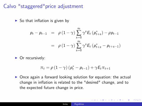
I So that in�ation is given by

pt � pt�1 = ρ (1� γ)∞

∑s=0

γsEt (p�t+s )� ρpt�1

= ρ (1� γ)∞

∑s=0

γsEt (p�t+s � pt+s�1)

I Or recursively:

πt = ρ (1� γ) (p�t � pt�1) + γEtπt+1

I Once again a forward looking solution for equation: the actualchange in in�ation is related to the "desired" change, and tothe expected future change in price.

Imbs Rigidities

Taking stock

I Price rigidities central to keynesian economics, i.e. to anymodel where there is a role for monetary policy.

I Rigorous treatment of nominal rigidities requires that �rmscan set their price, i.e. that they have market power.

I The "Dixit-Stiglitz" approach (i.e. monopolistic competitionbetween imperfect substitutes) made it possible to model thatrigorously.

I Imperfect substitutes can be either on the consumption or onthe production side.

I Gives rise to markups over marginal costs.I And to forward looking behavior of in�ation - akin to what wesaw in "expectations augmented Phillips curves"

Imbs Rigidities