Embed Size (px)
Citation preview

NON-ADDITIVE MARKET DEMAND FUNCTIONS:
PRICE ELASTICITIES WITH BANDWAGON, SNOB
AND VEBLEN EFFECTS
Amy Heineike and Paul Ormerod
Abstract
In a remarkable article published in 1950, Leibenstein extended the standard theory of consumer
demand by relaxing the assumption that the consumption of any individual is independent of
others. We discover important qualifications to Leibenstein’s findings on price elasticity in the
presence of Bandwagon, Snob and Veblen effects, though in general they are confirmed. We
then analyse the impact of assuming that consumers are connected on networks other than the
completely connected graph implicitly assumed by Leibenstein. The results are surprisingly
resilient to assumptions about network topology, although for any level of price, demand is lower
when the assumption of complete connectivity is relaxed.
Keywords: consumer demand theory; non‐additive; networks; bandwagon, snob and Veblen effects
JEL classification: D11, D82, D85
1

1. Introduction
Standard consumer choice theory assumes atomised individuals exercise choice in an attempt to
maximise utility subject to a budget constraint. In this approach, given an individual’s tastes and
preferences, decisions are taken on the basis of the attributes of the various products, such as price and
quality.
In recent decades, the conventional theory has of course been extended to allow for factors such as the
cost of gathering information (Stigler 1961), asymmetric information across agents (Akerlof 1970),
imperfections in the perception of information and limitations to consumers’ cognitive powers in
gathering and processing information (Simon 1955). So decisions are not necessarily made in a fully
rational way, but are nevertheless based on the (perceived) attributes of the products, without direct
reference to the choices of others. (Of course, the latter can affect choice indirectly by their effect on
relative prices.)
In a remarkable article published in 1950, Leibenstein made important steps in extending the standard
theory of consumer demand in what is arguably an even more fundamental way. He relaxed the
assumption that the consumption of any individual is independent of the consumption of others and
considered the implications for market demand curves of such behaviour.
Leibenstein pointed out that there was a literature, going back over a century even at the time at which
he wrote, in which the utility function of one individual contains the quantities of goods consumed by
other individuals. Leibenstein’s contribution was to analyse this in a formal way for the first time. He
2

examined how the price elasticity of the market demand function is affected by non‐additive
preferences.
Leibenstein identified three key ways in which the decisions of others might impact directly on the
behaviour of an individual and hence affect the price elasticity of the market demand curve. First, the
‘bandwagon’ effect, defined as being when the demand for a commodity is increased due to the fact
that others are also consuming the same commodity. There is, of course, a large and growing literature
on this phenomenon across a wide range of practical examples (for example, Schelling 1973, Arthur
1989, De Vany and Wallis 1996, Salganik et.al. 2006, Ormerod 2007). However, such literature usually
focuses solely on this social influence effect – termed ‘binary choice with externalities’ by Schelling –
and neglects the role of price.
Less has been written on Leibenstein’s other channels of influence, namely what he terms ‘snob’ and
‘Veblen’ effects. By the snob effect, he refers to the extent to which the demand for a product is
decreased owing to the fact that others are also consuming the same product. And by the Veblen
effect, he means the extent to which the demand for a product is increased because it bears a higher
rather than a lower price. The former is a function of the consumption of others, the latter is a function
of price.
A wider literature on non‐additive preferences has developed, but this research does not draw out the
implications for the price elasticity of the market demand function. Becker (1974), for example,
proposed a theory of social interactions in which the individual can, by his or her decisions, alter the
monetary value to the agent of the relevant characteristics of others, but did not examine the
consequences for aggregate demand curves. Pollack (1976) examined a model in which individual
3

demand is positively related to the past consumption of other agents – a form of bandwagon effect –
but his focus was on the impact of the distribution of income and expenditure on consumption, and not
on the impact of interactions on aggregate price elasticity. Basman et.al. (1988) suggest that post‐World
War Two consumer expenditure data offer support for Veblen’s hypothesis on preference formation.
Bagwell and Bernheim (1996) argue that if Veblen effects exist, traditional analysis of taxation policy can
lead to highly misleading conclusions. Hopkins and Kornienko (2004) analyse the Veblen effect in the
context of Nash equilibrium to show, perhaps unsurprisingly, that each individual spends an inefficiently
high amount on the status good.
Leibenstein drew three conclusions about the shape of the market demand curve: First, if the
bandwagon effect is the most significant effect, the demand curve is more elastic than it would be if this
external consumption effect were absent. Second, if the snob effect is the predominant effect, the
demand curve is less elastic than otherwise. Third, if the Veblen effect is the predominant one, the
demand curve is less elastic than otherwise, and some portions of it may even be positively inclined;
whereas, if the Veblen effect is absent, the curve will be negatively inclined regardless of the importance
of the snob effect in the market.
There are two main purposes of the paper. Firstly, to analyse the validity of Leibenstein’s conclusions
using, as he implicitly did, a completely connected network. Secondly, to check their robustness by
extending the analysis to consider three types of network which research, primarily over the last
decade, has shown to be particularly important in social, economic and cultural contexts, that is the
scale free, small world and random networks.
4

Section 2 gives a brief overview of networks. Section 3 describes the model, and the section 4 shows
the results of introducing the Veblen effect, since this extension of the standard demand model is least
affected by network configuration. Section 5 describes the impact of the bandwagon and snob effects
with a completely connected network, making them directly comparable to those of Leibenstein.
Section 6 introduces the effects of different networks. In economic terms in this context, networks
which are not completely connected introduce asymmetries into the sets of information which different
agents use in their purchase decisions.
2. Networks: an overview
An implicit assumption made by Leibenstein is that the consumers are connected in what would now be
described as a completely connected network. We describe agents as being connected if the decision of
one enters into the demand function of the other. So on a completely connected network, the decision
of any given agent is affected by the decisions of every other agent.
In economic terms, we can obviously think of this as implying that agents have access to complete
information about the decisions of others. In social terms, it means that they not only have access to
this information, but that they choose to take everyone else’s decision into account.
The assumption of a completely connected network is a particularly restrictive one in the light of recent
theoretical and empirical advances in networks. (A valuable introduction to recent socio‐economic uses
of network theory is Durrett 2006). For our purposes, we consider networks where any given agent is
only connected to a subset of all others. Again, we can think of this in economic terms as being a
situation of asymmetric information in that agents have access to different information about the
5

decisions of others, or we can think of it in social terms as meaning that agents choose to take account
of only a subset of all other agents.
First, a random network, in other words, any given agent is connected to another (i.e. takes account of
the decisions of the other) at random with probability p. At first sight it might seem an unusual
assumption to make in a social context. But the assumption that agents are connected at random is
made by many standard models of epidemiology (for example Murray 1989), and random copying has
been shown to offer a good explanation of data patterns observed in the evolution of tastes (for
example, Bentley and Shennan 2005, Shennan and Wilkinson 2001).
Second, a small world network (Watts and Strogatz 1998), such networks can essentially be thought of
as overlapping groups of ‘friends of friends’ and have been shown to be important in social and
economic contexts (for example, Ormerod and Wiltshire 2009). Small world networks consist of a
network of vertices whose topology is that of a regular lattice, with the addition of a low density of
connections between randomly‐chosen pairs of vertices. This latter can be either an addition to the
connections on a regular lattice or can replace the relevant number of such connections.
Third, a scale free network, these are networks whose degree distribution follows a power law, at least
asymptotically. That is, the fraction P(k) of nodes in the network having k connections to other nodes is
distributed for large values of k as P(k) ~ k−γ. Empirical examples include the distributions of both
internet links (Barabási‐Albert 1999) and sexual partners (Liljeros et al., 2001).
6

3. The theoretical model
We consider the demand for a consumer product and populate the model with N consumers. The basic
demand function for each agent is well behaved:
Ui = ai – P (1)
Choice: wi = 1 (buy) if Ui >0, or
0 otherwise
The ai are selected at random and represent the heterogeneous tastes of the agents. The sum of the
individual demands wi represents the market demand. We assume that the size of the market is small
compared to consumers’ incomes and can therefore reasonably ignore the difficulties which the
Sonneschein‐Mantel‐Debreu theorems (for example Sonnenschein 1972) raise for the shape of
aggregate demand functions. The demand curves for each individual agent are well‐behaved, and we
assume that the sum of these is also well‐behaved.
For convenience, we bound P in [0,1]. We assign an ai at random to each agent and then vary the level
of P to obtain the overall demand at different levels of price. We solve the model a number of different
times, each time with a different random draw for the values of the ai, and present results averaging
across all of the individual model solutions. In the results below we set N = 1000, and carry out 100
separate solutions of each variant of the model.
The exact shape of the market demand curve using (1) varies depending upon the distribution from
which the ai are drawn. For example, drawing from a normal distribution with mean = 0.5 and standard
deviation = 0.1, we obtain a market demand curve which resembles an S‐shaped curve in reverse, but
7

which is nevertheless downward sloping throughout with respect to price. The most straightforward
result is obtained when the ai are drawn from a uniform distribution on [0,1], when the market demand
curve is a linear throughout. We use this assumption in the results below, since its simplicity makes
comparisons clearer with more complicated versions of (1). Figure I shows the aggregate demand curve
under these assumptions. We represent demand as the proportion of all consumers who buy, so this
varies between 0 and 1.
To introduce the bandwagon and snob model we change the U function to:
U(i,t) = ai –P + ci*Zi (t‐1) (2)
where Zi (t‐1) = proportion of neighbours of agent i buying the product at time (t‐1)
in the bandwagon model ci > 0, and for the snob model ci < 0
The ‘neighbours’ of agent i are defined as being the agents to which that agent is connected i.e. he or
she pays attention to their decisions.
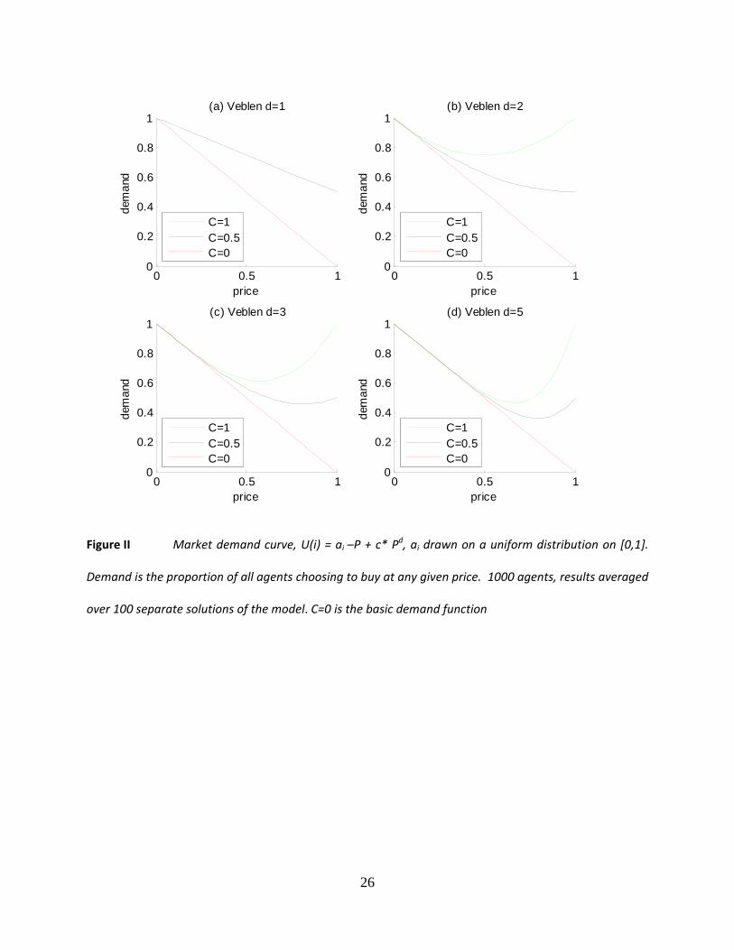
The Veblen effect is introduced as follows:
U(i) = ai –P + c* Pd (3)
In other words, overlaying the standard negative effect of price on demand is a further term which
leads to demand increasing as price rises, enabling consumers to display conspicuous consumption.
8

where we examine the effects of selecting different values of c and d, where d is the exponent of P.
We assume that these take the same values across all agents, though an extension would be to allow
for these to vary across agents.
4. The Veblen effect
This is straightforward to analyse, and the conclusions are identical to those of Leibenstein. Note in
addition that (3) does not depend on the structure of the network on which the agents are connected, it
is purely a function of price. Figure II sets out a selection of results. The results where c = 0 are simply
those of the basic demand function (1) and are included for purposes of comparison.
5. Bandwagon and snob effects on a completely connected network
The results in this section are obtained with a completely connected network, in other words each agent
is assumed to pay attention to the purchase decisions of all others. This is the assumption made in the
original Leibenstein paper, although at the time it was not described in network terms.
There are two technical aspects of the model to consider in simulations of equation (2). First, whether
in any given step of the model agents make decisions in sequence or simultaneously. In the latter, all
agents consider the external demand effect in the previous period, Z (t‐1), and the price in the current
period, and make their decisions on the basis of this information.
In the former, an agent is chosen at random to make a decision on the basis of this same information.
However, the sampling is continued without replacement until the decisions of all agents at time (t) are
9

known. So in this case, apart from the first agent chosen at random, agents receive increasing amounts
of information about external demand at time (t).
The second point relates to the initial conditions which we assume for external demand, Z, at time zero.
In principle this could take any value between 0 and 1, and we examine the sensitivity to results to this
assumption.
Bandwagon
The results obtained when this effect is taken into account are in fact robust with respect to both of the
technical points made above. The only point to note is that if Z(0) is assumed to equal 1, for high C and
P=1, a second solution of demand equal to 1 can be seen. This reflects a situation where everyone will
purchase if and only if everyone else purchases.
In general, the results confirm those of Leibenstein, with a distinct refinement. Figure III plots the
results for when external demand Z takes an initial value of zero.
The results are in line with those shown by Leibenstein. The important difference is that while he states
that this means:
(1) If the bandwagon effect is the most significant effect, the demand curve is more elastic than it
would be if this external consumption effect were absent.
10

There are actually two distinct regions in which the effects take hold. At first, price increases are not
matched by demand falls since the presence of a large pool of external demand creates a bandwagon
effect that keeps the demand high. At low prices, therefore, demand is completely inelastic. After a
certain critical point, however, the demand curve becomes more elastic, as consumers are deterred not
only by price, but of the loss of demand from other consumers at the same time. The point is
determined by the strength of the bandwagon effect.
Snob
The results here are sensitive to the assumption which is made about the order in which agents choose,
or, to put this into an economic context, the information set which agents have when making their
choices. If all agents decide simultaneously using information solely on P(t) and Z(t‐1), the model
oscillates and never settles to a solution. Allowing agents to choose in sequence and updating the
information on Z does give stable solutions. The exact shape of the demand curve given the ai and ci is
slightly sensitive to the order in which the agents choose, so no two solutions are exactly identical, but
in general there is very little difference between any two separate solutions.
In this case, apart from the above point, the results match exactly those of Leibenstein, namely: ‘If the
snob effect is the predominant effect, the demand curve is less elastic than otherwise.‘
For low prices, the snob effect suppresses demand, as price rises, demand falls but the extent of the
demand suppression falls leading to a smaller elastic effect at all price levels.
11

6. Alternative assumptions about agent networks
Here we consider the effects of network types which are known to be empirically important, and in
which agents do not take into the account the decisions of all other agents. Again, to repeat, this could
arise either because agents have asymmetric information and are not aware of the decisions of all other
agents, or because they choose not to take account of the decisions of other agents even though they
may have this information.
There is a very wide range of network types and parameterisations which could be considered. But the
task can be bounded in two ways. First, as already noted, we limit our examination of network types to
three which are known to be important in social and economic contexts, namely random, small world
and scale free.
Second, in terms of the bandwagon and snob effects, our interest is in how the decisions of each agent
are affected by those of the other agents to which he or she pays attention. In the completely
connected network, each agent takes account of what everyone else has done. Our interest is in
examining the effect on market demand functions when agents are influenced by the decisions of only a
sub‐set of the total number of other agents. This immediately restricts the range of parameters of each
kind of network to be examined, since a wide range of values will lead to the formation of a giant cluster
in the network, when the network then approximates the properties of a completely connected
network. So it is only worth examining relatively low values of the relevant parameters.
A way of formalising the similarity of any given network parameterisation to that of a completely
connected network is to calculate the average path length of the network. Average path length is a
12

fundamental concept in graph theory, and defines the average number of steps along the shortest path
for all possible pairs of network nodes. It is a measure of the efficiency with which, for example,
information can percolate across a network, the shorter the average path length the more efficient it is.
For a completely connected network, the average path length is by definition equal to 1. Each agent is
connected directly to every other agent.
We therefore focus our analysis on the effect on the market demand function of different values of the
average path length of the network. We illustrate this in two ways. First, using a random network and
varying the probability that any two agents are connected is varied (by ‘connected’, we mean in the
economic context that an agent pays attention to the purchase decision of the other). Secondly, by
examining the effect of different kinds of network.
The results are illustrative and further work could undoubtedly be carried out, but a clear pattern
emerges.
Table I sets out the typical average path length of a random network when the probability of connection
between agents is varied.
These calculations are performed for a network containing 1000 agents. The average path length does
vary with the number of nodes (agents) in the network, but not dramatically. The scaling is around
log(n) for the random network, with small world scaling between log(n) and n depending on the value of
p , and scale free scaling of order (log(n)/loglog(n)) (Albert and Barabasi 2002).
Figure V shows the results obtained using a random network with different values of the probability of
connection when the bandwagon effect is assumed to exist.
13

The networks show similar behaviour to that of a completely connected network, but with lower
demand for any given price in each case. Further, the lower the value of the average path length, the
closer the demand curve becomes to that of the completely connected network and, conversely, the
higher it is the more the demand curve begins to approximate that when there are no network effects
present at all.
The rationale for this is straightforward. In equation (2), any given agent is only influenced in his or her
immediate purchase decision by a subset of other agents, Z(i,t). When the size of Z(i,t) is larger it is
more likely that when one agent changes to a purchasing decision, there is another agent within Z(i,t)
who was close enough to wanting to purchase that the agent’s choice pushed them to decide to
purchase too. Increasing the connectivity of the network can therefore facilitate cascades of behaviour
where individuals are influenced by their neighbours and in turn influence more neighbours. Long
average path length indicates that these cascades are likely to be broken, since the cascade becomes
dependent on agents who can be influenced easiest being directly connected together and agents with
low preference for the product being somehow out of the way.
Table II shows average path lengths for various parameterisations of the other types of networks we
consider. We in normalise the comparisons by choosing parameters such that the average degree in
each network is equal to 4. The model is again populated by 1000 agents.
Figure VI plots the results.
14

The lowest demand occurs for small world, followed by scale free and then the random network. We
see that the small world network, which in this case has a very long average path length, is indeed
furthest from the complete network in final demand. However the order between the scale free
network and the random network is surprising since the scale free has shorter average path length than
the random network and therefore could be expected to transmit information more efficiently.
This can be understood by considering how agents with very large numbers of connections, the hubs, in
the scale free network behave. Hubs are very difficult to influence, since the scale of impact is
measured by the proportion of their neighbours who purchase and they have many neighbours. Once
they have decided to purchase, however, they are able to heavily influence many other agents, since
they are likely to represent a significant proportion of their neighbour’s connections. Therefore, while
hubs are important in reducing path length, they are not efficient transmitters of purchasing decisions.
Final overall demand is likely to be very dependent on whether those individuals happened to have a
high initial preference for the product.
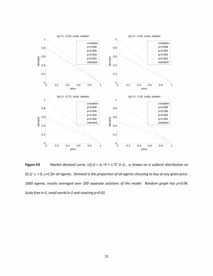
For the snob model in Figures VII and VIII we see a similar dynamic at work, although the differences
appear to be less pronounced. Networks with long average path lengths end with a final demand more
similar to one in which no network effects are present, while the more connected networks approach
the results of the complete network.
The difference between networks becomes even less apparent when we compare the different network
types. In the bandwagon model there is a strong positive feedback which can extenuate the differences
between similar initial conditions. For the snob model, however, the feedback is negative, which means
15

that any increase in purchasing in one part of the network is matched by a decline in purchasing
elsewhere. It is therefore very difficult to find a network configuration which would change the final
demand from that of the complete network to any large extent. The largest deviations occur when
there are few connections between agents, the price is high and demand is low. In these cases the
snobs can be insulated from each other, so that they do not reduce their demand in response to
knowledge that other people are in fact making the same purchasing decisions as them. In this case any
lowering of the number of connections is an effective enabler of demand.
7. Conclusion
Sociologists for a long time have emphasised the importance of interactions with other agents in the
evolution of individual preferences. The relevant literature in economics is rather sparse, and the
assumption of independent preferences and additive market demand functions is still used widely by
economists in practice. Increasingly, however, as information about the behaviour and tastes of other
agents becomes much more readily available through, for example, the internet, the assumption of
completely independent individual preferences becomes less realistic in a wide range of consumer
markets.
As long ago as 1950, Leibenstein analysed the implication for market demand functions, and in
particular price elasticities, when individual preferences are non‐additive. He examined three distinct
ways in which agents might interact in the shaping of preferences. The ‘bandwagon’ and ‘snob’ effects,
when the demand for a commodity by an agent is, respectively, increased or decreased due to the fact
that others are also consuming the same commodity. And the Veblen effect, which he defined as the
16

extent to which the demand for a product is increased because it bears a higher rather than a lower
price.
Leibenstein assumed that each agent takes into account the preferences of all other agents in forming
his or her decision. So that agents not only have information about the behaviour of all others, but they
take this into account in their own decisions. In the modern terminology of graph theory, the agents
form a completely connected network.
We find that in general, under these assumptions, that Leibenstein’s results bear scrutiny, but with
some important qualifications. For example, under the assumption of a bandwagon effect, the demand
curve is more elastic than it would be if this external consumption effect were absent. But there are
actually two distinct regions in which the effects take hold. At first, price increases are not matched by
demand falls since the presence of a large pool of external demand creates a bandwagon effect that
keeps the demand high. At low prices, therefore, demand is completely inelastic. After a certain critical
point, however, the demand curve becomes more elastic, as consumers are deterred not only by price,
but of the loss of demand from other consumers at the same time. The point is determined by the
strength of the bandwagon effect.
For the snob effect, the results match exactly those of Leibenstein, namely: ‘If the snob effect is the
predominant effect, the demand curve is less elastic than otherwise.‘ However, the results here are
sensitive to the assumption which is made about the order in which agents choose, or, to put this into
an economic context, the information set which agents have when making their choices. If all agents
decide simultaneously using information solely on current price and the preferences on all other agents
in the previous period, the model oscillates and never settles to a solution. Allowing agents to choose in
17

sequence and updating the information available to each agent on the preferences of others does give
stable solutions.
We extend the analysis by connecting agents on three types of network which have been shown
recently to be important in social, cultural and economic contexts, namely a random network, a small
world network and a scale‐free network.
In these types of network, agents do not take into the account the decisions of all other agents. This
could arise, for example, because agents have asymmetric information and are not aware of the
decisions of all other agents, or because they choose not to take account of the decisions of other
agents even though they may have this information.
A way of formalising the similarity of any given network parameterisation to that of a completely
connected network is to calculate the average path length of the network. Average path length is a
fundamental concept in graph theory, and defines the average number of steps along the shortest path
for all possible pairs of network nodes. It is a measure of the efficiency with which, for example,
information can percolate across a network, the shorter the average path length the more efficient it is.
We focus our analysis on the effect on the market demand function of different values of the average
path length of the network. We illustrate this in two ways. Firstly, using a random network and varying
the probability that any two agents are connected is varied (by ‘connected’, we mean in the economic
context that an agent pays attention to the purchase decision of the other) and secondly, by examining
the effect of different kinds of network.
18

The results are illustrative and further work could undoubtedly be carried out, but a clear pattern
emerges. With either the bandwagon or snob effect assumed to exist (the Veblen effect depends simply
on price and so the network structure has no effect), the networks show similar behaviour to that of a
completely connected network, but with lower demand for any given price in each case. Further, the
lower the value of the average path length, the closer the demand curve becomes to that of the
completely connected network and, conversely, the higher it is the more the demand curve begins to
approximate that when there are no network effects present at all.
There is a difference between the bandwagon and snob effects. In the bandwagon model there is a
strong positive feedback which can extenuate the differences between similar initial conditions. For the
snob model, however, the feedback is negative, which means that any increase in purchasing in one part
of the network is matched by a decline in purchasing elsewhere. It is therefore very difficult to find a
network configuration which would change the final demand from that of the complete network to any
large extent. The largest deviations occur when the price is very high and so demand is very low, and it
is easier to insulate snobs from knowledge that other people are in fact making the same purchasing
decisions as them.
The results are therefore surprisingly resilient to the assumptions made about network topology,
although for any given level of price, overall demand is lower when the assumption of complete
connectivity is relaxed.
Perhaps the most important practical implication of this analysis is that in the presence of bandwagon
effects – which clearly exist in many markets especially those related to popular culture – the market
demand curve is horizontal over rather large ranges of price. The task for companies involved in such
19

markets is to discover the point at which price begins to dominate network effects, and to price
accordingly.
1. Amy Heineike, [email protected]; Centre for Social Complexity, George Mason
University, Fairfax, VA, USA
2. Paul Ormerod, [email protected]; Volterra Consulting, 135c Sheen Lane,
London SW14 8AE, UK
References
Akerlof, G.A. “The market for ‘lemons': Quality uncertainty and the market mechanism.” Quarterly
Journal of Economics, 84 (1970), 488‐500
Albert,R., and Barabasi, A.L.. “Statistical mechanics of complex networks.” Reviews of Modern Physics
,74 (2002), 47–97
Amaral, L.A.N., Scala,A, Barthélémy, M. and Stanley, H.E. “Classes of small world networks”, Proceedings
of the National Academy of Science, (2000) 11149‐52
Arthur,W.B. “Competing technologies, increasing returns, and lock‐in by historical events.” Economic
Journal ,99 (1989), 116‐131.
Bagwell L.S. and Bernheim B.D. “Veblen effects in a theory of conspicuous consumption.” American
Economic Review, 86 (1996), 349‐373
Barabási A.L. and Albert, R. “ Emergence of scaling in random networks.” Science, 286 (1999), 509‐512
20

Basmann R.L., Molina D.J. and Slottje D.J.. “ A note on measuring Veblen's theory of conspicuous
consumption.” Review of Economics and Statistics, 70 (1988), 531‐535
Becker G.S. “A theory of social interactions.” Journal of Political Economy, 82 (1974), 1063‐1093
Bentley, R.A. and Shennan, S.J. “Random copying and cultural evolution.” Science, 309 (2005), 877‐879
deVany, A. and Wallis, R. “Bose‐Einstein dynamics and adaptive contracting in the motion picture
industry”. Economic Journal, 106 (1996), 1493‐1514
Durrett, R. Random Graph Dynamics (Cambridge University Press, 2006)
Hopkins, E. and Kornienko, T. “Running to keep in the same place: consumer choice as a game of
status.” American Economic Review, 94 (2004), 1085‐1107
Leibenstein, H. “Bandwagon, Snob, and Veblen Effects in the theory of consumers' demand.” Quarterly
Journal of Economics, 64 (1950), 183‐207
Liljeros, F., Edling, C.R., Amaral, L.A.N., Stanley, H.E. and Aberg, Y. “The web of human sexual contacts.”
Nature, 411 (2001), 907‐908
Murray, J.D. Mathematical Biology. (Springer‐Verlag, Berlin, 1989)
Ormerod, P., and Wiltshire G.. Binge drinking in the UK: a social network phenomenon. Mind and
Society, forthcoming (2009)
Ormerod, P. “Extracting deep information from limited observations on an evolved social network.”
Physica A, 378 (2007), 48‐52
Pollak R.A. “Interdependent preferences.” American Economic Review, 66 (1976), 309‐320
Salganik M.J., Dodds, P.S., and Watts, D.J. “Experimental study of inequality and unpredictability in an
artificial cultural market.” Science, 311 (2006), 854‐856
Schelling T.C. “Hockey helmets, concealed weapons, and daylight saving: a study of binary choices with
externalities,” Journal of Conflict Resolution, 13 (1973), 381‐428
21

Shennan S.J., and Wilkinson, J.R. “Ceramic style change and neutral evolution: A case study from
Neolithic Europe.” American Antiquity, 66 (2001), 577‐594
Simon H.A. “A behavioural model of rational choice.” Quarterly Journal of Economics, 69 (1955), 99‐118
Sonnenschein H. “Market excess demand functions.” Econometrica, 40 (1972), 549–563
Stigler, G.J. “The economics of information.” Journal of Political Economy, 69 (1961), 213‐225
Watts, D.J., and Strogatz, S.H. “Collective dynamics of “small‐world” networks’,” Nature, 393 (1998),
440‐442
22

TABLES
Table I Comparison of mean path lengths for a random network (averaged over 10 generated networks)
Random network, p of
connection (with
N=1000)
0.002 0.004 0.006 0.008 1 (Complete
Network)
Mean Path Length 9.29 5.22 4.08 3.57 1
23

Table II Comparison of mean path lengths for the network models used in the network. All apart from
the complete network have a mean degree of 4.
Network (with
N=1000)
Small World
(k=2,p=0.01)
Random
(p=0.004)
Scale free
(k=2,m=2) Complete
Mean path length 19.63 5.22 4.10 1
24

FIGURES
0 0.2 0.4 0.6 0.8 10
0.1
0.2
0.3
0.4
0.5
0.6
0.7
0.8
0.9
1
price
dem
and
Standard Model, ai distributed uniformly on (0,1)
Figure I Market demand curve, Ui = ai – P, ai drawn on a uniform distribution on [0,1]. Demand is the
proportion of all agents choosing to buy at any given price. 1000 agents, results averaged over 100
separate solutions of the model
25
0 0.5 10
0.2
0.4
0.6
0.8
1
price
dem
and
(a) Veblen d=1
C=1C=0.5C=0
0 0.5 10
0.2
0.4
0.6
0.8
1
price
dem
and
(b) Veblen d=2
C=1C=0.5C=0
0 0.5 10
0.2
0.4
0.6
0.8
1
price
dem
and
(c) Veblen d=3
C=1C=0.5C=0
0 0.5 10
0.2
0.4
0.6
0.8
1
price
dem
and
(d) Veblen d=5
C=1C=0.5C=0
Figure II Market demand curve, U(i) = ai –P + c* Pd, ai drawn on a uniform distribution on [0,1].
Demand is the proportion of all agents choosing to buy at any given price. 1000 agents, results averaged
over 100 separate solutions of the model. C=0 is the basic demand function
26

0 0.2 0.4 0.6 0.8 10
0.1
0.2
0.3
0.4
0.5
0.6
0.7
0.8
0.9
1
price
dem
and
Bandwagon model
C=1.25C=1
C=0.75
C=0.5
C=0.25C=0
Figure III Market demand curve, U(i,t) = ai –P + ci*Zi (t‐1) , ai drawn on a uniform distribution on
[0,1] ci > 0, ci=C for all agents. Demand is the proportion of all agents choosing to buy at any given price.
1000 agents, results averaged over 100 separate solutions of the model
27

0 0.2 0.4 0.6 0.8 10
0.1
0.2
0.3
0.4
0.5
0.6
0.7
0.8
0.9
1
price
dem
and
C=1.25C=1C=0.75C=0.5C=0.25C=0
Figure IV Market demand curve, U(i,t) = ai –P + ci*Zi (t‐1) , ai drawn on a uniform distribution on
[0,1] ci <0 , ci=C for all agents. Demand is the proportion of all agents choosing to buy at any given price.
1000 agents, results averaged over 100 separate solutions of the model
28

0 0.2 0.4 0.6 0.8 10
0.2
0.4
0.6
0.8
1
price
dem
and
(a) C=0.25, bandwagon, random
completep=0.008
p=0.006
p=0.004
p=0.002standard
0 0.2 0.4 0.6 0.8 10
0.2
0.4
0.6
0.8
1
price
dem
and
(a) C=0.50, bandwagon, random
completep=0.008
p=0.006
p=0.004
p=0.002standard
0 0.2 0.4 0.6 0.8 10
0.2
0.4
0.6
0.8
1
price
dem
and
(a) C=0.75, bandwagon, random
completep=0.008
p=0.006
p=0.004
p=0.002standard
0 0.2 0.4 0.6 0.8 10
0.2
0.4
0.6
0.8
1
price
dem
and
(a) C=1.00, bandwagon, random
completep=0.008
p=0.006
p=0.004
p=0.002standard
Figure V Market demand curve, U(i,t) = ai –P + ci*Zi (t‐1) , ai drawn on a uniform distribution on
[0,1 ci < 0, ci=C for all agents. Demand is the proportion of all agents choosing to buy at any given price.
1000 agents, results averaged over 100 separate solutions of the model. Results for random network
with probability of connection=p.
29

0 0.2 0.4 0.6 0.8 10
0.2
0.4
0.6
0.8
1
price
dem
and
(a) C=0.25 bandwagon
Small World
Scale Free
RandomComplete
Standard
0 0.2 0.4 0.6 0.8 10
0.2
0.4
0.6
0.8
1
price
dem
and
(b) C=0.5 bandwagon
Small World
Scale Free
RandomComplete
Standard
0 0.2 0.4 0.6 0.8 10
0.2
0.4
0.6
0.8
1
price
dem
and
(c) C=0.75 bandwagon
Small World
Scale Free
RandomComplete
Standard
0 0.2 0.4 0.6 0.8 10
0.2
0.4
0.6
0.8
1
price
dem
and
(d) C=1 bandwagon
Small World
Scale Free
RandomComplete
Standard
Figure VI Market demand curve, U(i,t) = ai –P + ci*Zi (t‐1) , ai drawn on a uniform distribution on
[0,1 ci < 0, ci=C for all agents. Demand is the proportion of all agents choosing to buy at any given price.
1000 agents, results averaged over 100 separate solutions of the model. Random graph has p=0.04,
Scale free k=2, small world k=2 and rewiring p=0.01.
30
0 0.2 0.4 0.6 0.8 10
0.2
0.4
0.6
0.8
1
price
dem
and
(a) C= -0.25, snob, random
completep=0.008
p=0.006
p=0.004
p=0.002standard
0 0.2 0.4 0.6 0.8 10
0.2
0.4
0.6
0.8
1
price
dem
and
(a) C= -0.50, snob, random
completep=0.008
p=0.006
p=0.004
p=0.002standard
0 0.2 0.4 0.6 0.8 10
0.2
0.4
0.6
0.8
1
price
dem
and
(a) C= -0.75, snob, random
completep=0.008
p=0.006
p=0.004
p=0.002standard
0 0.2 0.4 0.6 0.8 10
0.2
0.4
0.6
0.8
1
price
dem
and
(a) C= -1.00, snob, random
completep=0.008
p=0.006
p=0.004
p=0.002standard
Figure VII Market demand curve, U(i,t) = ai –P + ci*Zi (t‐1) , ai drawn on a uniform distribution on
[0,1] ci < 0, ci=C for all agents. Demand is the proportion of all agents choosing to buy at any given price.
1000 agents, results averaged over 100 separate solutions of the model. Random graph has p=0.04,
Scale free k=2, small world k=2 and rewiring p=0.01.
31

0 0.2 0.4 0.6 0.8 10
0.2
0.4
0.6
0.8
1
price
dem
and
(a) C= -0.25 snob
Small World
Scale Free
RandomComplete
Standard
0 0.2 0.4 0.6 0.8 10
0.2
0.4
0.6
0.8
1
price
dem
and
(b) C= -0.5 snob
Small World
Scale Free
RandomComplete
Standard
0 0.2 0.4 0.6 0.8 10
0.2
0.4
0.6
0.8
1
price
dem
and
(c) C= -0.75 snob
Small World
Scale Free
RandomComplete
Standard
0 0.2 0.4 0.6 0.8 10
0.2
0.4
0.6
0.8
1
price
dem
and
(d) C= -1 snob
Small World
Scale Free
RandomComplete
Standard
Figure VIII Market demand curve, U(i,t) = ai –P + ci*Zi (t‐1) , ai drawn on a uniform distribution on
[0,1] ci < 0, ci=C for all agents. Demand is the proportion of all agents choosing to buy at any given price.
1000 agents, results averaged over 100 separate solutions of the model. Random graph has p=0.04,
Scale free k=2, small world k=2 and rewiring p=0.01.
32