Notes on Understanding GIS with an ArcView licensehelp.arcgis.com/en/ugis/pdf/UGIS with an ArcView license.pdfNotes on Understanding GIS with an ArcView license ... The Spatial Join

Notes on Understanding GIS with an ArcView license This document is a guide to completing the Understanding GIS project with an ArcView or ArcEditor license. In general, we used the following techniques to work around ArcInfo functionality: ArcInfo tools used in the book ArcView/ArcEditor substitute tools Erase Union Identity Intersect, Spatial Join Aggregate Polygons Merge (editing tool) Near Spatial Join ArcInfo extension used in the book ArcView/ArcEditor substitute functionality Maplex Convert labels to annotation Note: this shouldn’t be taken to mean that analysis results obtained with ArcInfo tools can always be achieved with tools in ArcView/ArcEditor: only that we could do it in this case. Overview Lessons 1 through 5, and Lesson 9, can be completed as written in the book with an ArcView or ArcEditor license. Changes need to be made to Lessons 6, 7, and 8.

Lesson Changes needed

1 none

2 none

3 none

4 none

5 none

6 see below

7 see below

8 see below

9 none

By and large, the workflow doesn’t change too much. There is, however, a change to the structure of the model in Lesson 7, as explained below in Exercise 7b, Step 4. Each of the exercises in Lessons 6 through 8 is listed below. Typically, most of the steps in an exercise don’t change; some steps have minor changes (such as different output feature class names) and some are partially or wholly rewritten. We’ve tried to provide sufficient detail on the steps, but there isn’t a lot of additional explanation or graphics.

Notes on Understanding GIS with an ArcView license

Ex6a: Establish proximity zones

Step 1: as is Step 2: as is Step 3: as is

Step 4: Erase park accessible areas Step 5: as is Step 4: Erase park accessible areas This step identifies areas that are within the river buffer but outside park buffers: in other words, areas we want to keep in consideration for a new park. In the book, this is accomplished with the Erase tool (ArcInfo license); here we’ll do it with the Union overlay tool (ArcView license). 4A In the Search window, find and open the Union (Analysis) tool. 4B For the Input Features, add the LARiverBuffer and Parks_Buffer layers. 4C Name the Output Feature Class ProximityZone. Click OK. 4D Open the attribute table of the ProximityZone layer. The table has three records, representing different spatial combinations. The first record, with an FID_LARiverBuffer value of 1 and an FID_Parks_Buffer value of -1, is the one we want. These are areas inside the river buffer and outside the parks buffers. 4E In the Table of Contents, right-click the ProximityZone layer and choose Edit Features > Start Editing. 4F Select the second and third records in the table and delete them. 4G Save edits and stop editing. Close the attribute table. 4H Turn off all layers except ProximityZone. 4I Symbolize ProximityZone in a medium blue color. The edited ProximityZone table has the same output achieved by the Erase tool in the book.


Ex6b: Apply demographic constraints

Step 1: Overlay block groups on the proximity zone Step 2: as is

Step 3: as is Step 4: as is

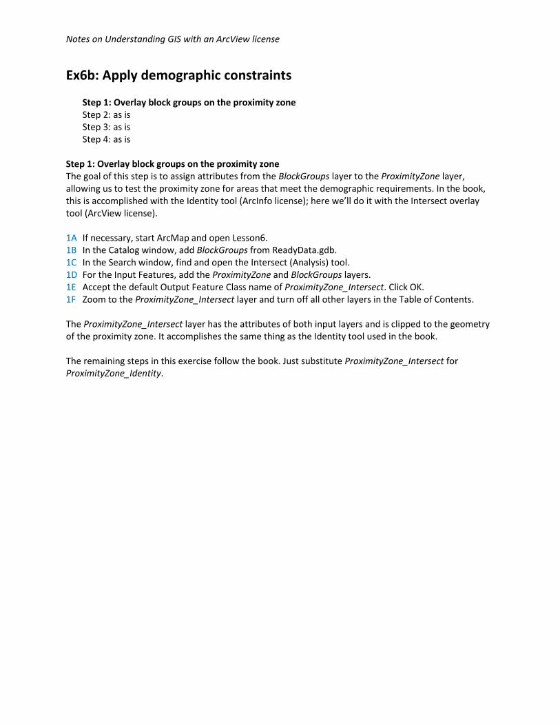
Step 1: Overlay block groups on the proximity zone The goal of this step is to assign attributes from the BlockGroups layer to the ProximityZone layer, allowing us to test the proximity zone for areas that meet the demographic requirements. In the book, this is accomplished with the Identity tool (ArcInfo license); here we’ll do it with the Intersect overlay tool (ArcView license). 1A If necessary, start ArcMap and open Lesson6. 1B In the Catalog window, add BlockGroups from ReadyData.gdb. 1C In the Search window, find and open the Intersect (Analysis) tool. 1D For the Input Features, add the ProximityZone and BlockGroups layers. 1E Accept the default Output Feature Class name of ProximityZone_Intersect. Click OK. 1F Zoom to the ProximityZone_Intersect layer and turn off all other layers in the Table of Contents. The ProximityZone_Intersect layer has the attributes of both input layers and is clipped to the geometry of the proximity zone. It accomplishes the same thing as the Identity tool used in the book. The remaining steps in this exercise follow the book. Just substitute ProximityZone_Intersect for ProximityZone_Identity.


Ex6c: Apply demographic constraints


Step 4: as is Step 5: Aggregate sites Step 6: Calculate acreage Step 7: Define park access zones

Step 8: as is Step 9: as is Step 10: Calculate distance to the river Step 11: Add the park-accessible layers to FiveSites Step 12: Add the demographic attributes to FiveSites_Identity

Step 5: Aggregate sites The goal in this step is to combine three candidate parcels separated by narrow easements into one parcel. In the book, the parcels are combined with the Aggregate Polygons tool (ArcInfo license); here, we’ll merge them in an edit session. 5A Zoom to the first record in the SevenSites attribute table, then close the table. 5B Zoom out slightly to see the three parcels that are near each other. 5C In the Table of Contents, right-click the SevenSites layer and choose Edit Features > Start Editing. 5D If necessary, open the Editor toolbar. 5E On the Editor toolbar, with the Edit tool selected, select the three parcels. 5F On the Editor toolbar, click the Editor drop-down button and choose Merge. 5G In the Merge dialog box, accept the default and click OK. 5H Save edits and stop editing. 5I Open the SevenSites attribute table. There are now five records, as desired. The three parcels have been merged into a single multipart feature. The result is a bit different from the book because you can still see three discrete boundaries (the three parts of the multipart feature). That’s fine, and we’ll leave it as is, although you could do more editing if you wanted to. For example, you could create a couple of new features to cover the gaps, then merge the new features with the existing feature to create a singlepart feature that would look like the one in the book.


Ex6c: Apply demographic constraints (continued)




Step 6: Calculate acreage In the book, the Aggregate Polygons tool created a new feature class with no acreage attribute, so we added a new field and then calculated its geometry. Here, we just have to recalculate the existing ACRES field. Note that in the book there’s both a SevenSites and a FiveSites feature class. (FiveSites is the output of Aggregate Polygons.) Here, we just have SevenSites. In the map document, we’ll rename the SevenSites layer to FiveSites. 6A In the SevenSites attribute table, right-click the ACRES field and choose Calculate Geometry. 6B In the Calculate Geometry dialog box, set the units to Acres US [ac]. Accept the other defaults and

click OK. 6C Close the attribute table. 6D In the Table of Contents, rename the SevenSites layer to FiveSites. Step 7: Define park access zones Skip Step 7A; otherwise, do the step as is.






Step 10: Calculate distance to the river In Step 10 in the book, we calculate the distance from each site to the river with the Near tool (ArcInfo license). Here, we can make that calculation with an optional parameter of the Spatial Join tool (ArcView license). The Spatial Join tool serves no purpose here except that distance calculation. It’s going to create a new feature class that’s the same as FiveSites, but with one additional field containing measurement values for distance to the river. Note: The Near tool used in the book doesn’t create a new feature class, but the Spatial Join tool does. So here we’ll create a new feature class that we didn’t create in the book. 10A Open the Spatial Join (Analysis) tool. 10B Set the Target Features to FiveSites and the Join Features to LARiver. 10C Name the Output Feature Class FiveSites. After we run the tool, we’ll replace the old FiveSites layer (which actually references the SevenSites feature class, as noted in Step 6D, above) with this one. 10D In the Field Map of Join Features area, delete all the fields except ACRES. 10E Set the Match Option to Closest. (This enables the Distance Field Name parameter.) 10F In the Distance Field Name box, type NEAR_DIST. This is a new field that will be created by the Spatial Join. You can use any Distance Field Name you like; we’re using NEAR_DIST just to maintain consistency with the book. 10G Click OK to run the tool. 10H Open the new FiveSites attribute table to see the NEAR_DIST field, then close the table. 10I Remove the old FiveSites layer (symbolized with a hollow fill and green outline) from the Table of

Contents.






Step 11: Add the park-accessible layers to FiveSites In Step 11, we assign the quarter-mile population values from the ParkAccessZones_SpatialJoin layer to the FiveSites layer. In the book, we did this with the Identity tool (ArcInfo license). Here, we’ll use the Spatial Join tool. 11A Open the layer properties for ParkAccessZones_SpatialJoin. 11B On the Fields tab, click the Turn all fields off button. 11C Check the POP2000 box to turn it back on. Click OK. 11D Open the Spatial Join tool. 11E Set the Target Features to FiveSites and the Join Features to Park Access Zones_Spatial Join. 11F Name the Output Feature Class FiveSitesWithPopCount. 11G In Field Map of Join Features, delete all fields except NEAR_DIST, ACRES, and POP2000. 11H Set the Match Option to WITHIN. (The default INTERSECT setting would also work.) 11I Click OK to run the tool. 11J Open the FiveSitesWithPopCount attribute table to confirm it has the key attributes, then close it. Step 12: Add the demographic attributes to FiveSites_Identity In Step 12, we assign demographic attributes from the BlockGroups layer to the FiveSites table. In the book, we used the Identity tool (ArcInfo license). Here, we’ll use Spatial Join again. 12A Open the layer properties for BlockGroups. 12B On the Fields tab, click the Turn all fields off button. 12C Turn MEDIAN HH INCOME, POP DENSITY, and PCT UNDER 18 back on. Click OK. 12D Open the Spatial Join tool. 12E Set the Target Features to FiveSitesWithPopCount and the Join Features to BlockGroups. 12F Name the Output Feature Class RecommendedSites. 12G In Field Map of Join Features, keep only these six fields: NEAR_DIST, ACRES, POP2000, MEDIAN HH

INCOME, POP DENSITY, and PCT UNDER 18. 12H Set the Match Option to WITHIN. (Again, INTERSECT would work here, too.) 12I Click OK to run the tool. 12J Open the RecommendedSites attribute table to confirm it has the key attributes, then close it. 12K Save the map document.


Ex6d: Clean up the map and geodatabase

Step 1: as is Step 2: as is Step 3: Delete unnecessary fields

Step 4: as is Step 5: as is Step 6: as is Step 7: as is Step 8: as is

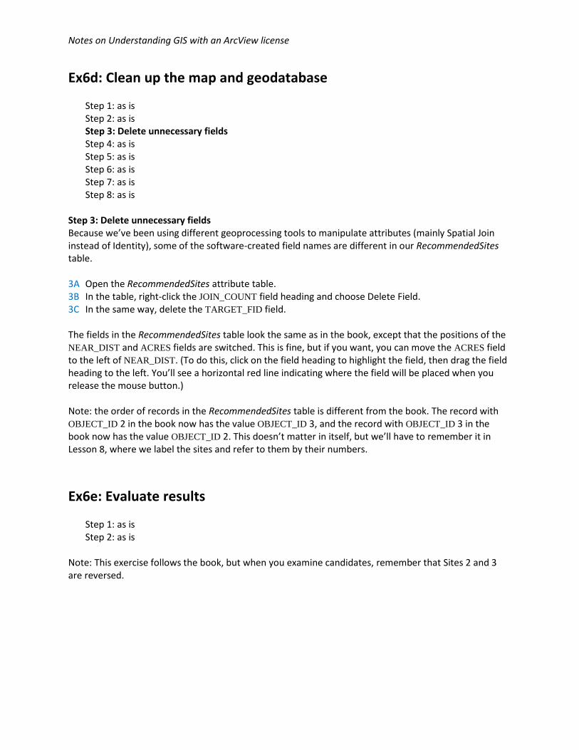
Step 3: Delete unnecessary fields Because we’ve been using different geoprocessing tools to manipulate attributes (mainly Spatial Join instead of Identity), some of the software-created field names are different in our RecommendedSites table. 3A Open the RecommendedSites attribute table. 3B In the table, right-click the JOIN_COUNT field heading and choose Delete Field. 3C In the same way, delete the TARGET_FID field. The fields in the RecommendedSites table look the same as in the book, except that the positions of the NEAR_DIST and ACRES fields are switched. This is fine, but if you want, you can move the ACRES field to the left of NEAR_DIST. (To do this, click on the field heading to highlight the field, then drag the field heading to the left. You’ll see a horizontal red line indicating where the field will be placed when you release the mouse button.) Note: the order of records in the RecommendedSites table is different from the book. The record with OBJECT_ID 2 in the book now has the value OBJECT_ID 3, and the record with OBJECT_ID 3 in the book now has the value OBJECT_ID 2. This doesn’t matter in itself, but we’ll have to remember it in Lesson 8, where we label the sites and refer to them by their numbers.

Ex6e: Evaluate results

Step 1: as is Step 2: as is Note: This exercise follows the book, but when you examine candidates, remember that Sites 2 and 3 are reversed.


Ex7a: Set up the model

Step 1: as is Step 2: as is Step 3: as is This exercise follows the book with no changes.

Ex7b: Build the model (Part 1)


Step 4: Erase park buffers Step 5: Assign block group demographics to the proximity zone Step 6: Validate and run the model

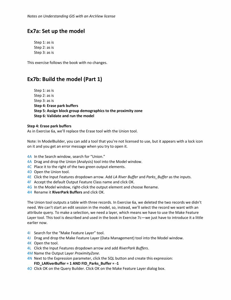
Step 4: Erase park buffers As in Exercise 6a, we’ll replace the Erase tool with the Union tool. Note: In ModelBuilder, you can add a tool that you’re not licensed to use, but it appears with a lock icon on it and you get an error message when you try to open it. 4A In the Search window, search for “Union.” 4A Drag and drop the Union (Analysis) tool into the Model window. 4C Place it to the right of the two green output elements. 4D Open the Union tool. 4E Click the Input Features dropdown arrow. Add LA River Buffer and Parks_Buffer as the inputs. 4F Accept the default Output Feature Class name and click OK. 4G In the Model window, right-click the output element and choose Rename. 4H Rename it RiverPark Buffers and click OK. The Union tool outputs a table with three records. In Exercise 6a, we deleted the two records we didn’t need. We can’t start an edit session in the model, so, instead, we’ll select the record we want with an attribute query. To make a selection, we need a layer, which means we have to use the Make Feature Layer tool. This tool is described and used in the book in Exercise 7c—we just have to introduce it a little earlier now. 4I Search for the “Make Feature Layer” tool. 4J Drag and drop the Make Feature Layer (Data Management) tool into the Model window. 4K Open the tool. 4L Click the Input Features dropdown arrow and add RiverPark Buffers. 4M Name the Output Layer ProximityZone. 4N Next to the Expression parameter, click the SQL button and create this expression: FID_LARiverBuffer = 1 AND FID_Parks_Buffer = -1 4O Click OK on the Query Builder. Click OK on the Make Feature Layer dialog box.


Ex7b: Build the model (Part 1) (continued)



Step 4: Erase park buffers (continued) At this point, we have a complication that we didn’t have in the book, although it’s kind of hard to explain until you run the model as a geoprocessing tool in Lesson 7d. The problem is this:

When we run the model as a tool, we’ll probably want to rerun it to experiment with alternative outcomes. For example, what happens if we make the river buffer a half mile? Or if we make the minimum park size five acres? Etc.

We want to preserve these various outcomes as separate datasets; we don’t want to keep overwriting previous results. There are different ways to do this, but the way we chose in the book was to store all the data in the same geodatabase (ModelBuilderOutputs) with different output file names.

One of the output files is the LA River buffer. That means that with each successive run of the model, we have to rename this file. For example, we’ll have LARiverBuffer, LARiverBuffer2, LARiverBuffer3, and so on.

A consequence of renaming this file is that each time the model runs and gets to the Union overlay (which uses the LA River buffer as an input), it creates a new field name for the attribute that references the LA River Buffer input: FID_LARiverBuffer, FID_LARiverBuffer2,

FID_LARiverBuffer3, and and so on.

At the same time, however, the expression in the Make Feature Layer tool that selects the appropriate record from the output of the Union overlay is hard-coded:

FID_LARiverBuffer = 1 AND FID_Parks_Buffer = -1.

The result is that the first time you run the model as a tool, it works properly. The second time, the Union tool generates a field name like FID_LARiverBuffer1, while the selection expression is looking for the field name FID_LARiverBuffer. This means that no selection gets made, which sabotages the model. It keeps running, but it can’t find any recommended sites because no area has been specified for it to look in.

There are different ways to solve this problem. The more elegant way (passing a variable to update the selection expression) is more complicated. Our solution is to make a copy of the LA River Buffer output. The original remains the input to the Union tool and isn’t renamed, so the selection expression works. The copy isn’t involved in subsequent processing and becomes the output feature class that gets renamed with each model run and written to the ModelBuilderOutputs geodatabase. 4P Search for the Copy Features (Data Management) tool and add it to the Model window. 4Q Open the tool. 4R Set the Input Features to LA River Buffer. 4S Name the Output Feature Class LARiverBufferDisplay and click OK. 4T Rename the output element LA River Buffer Display and click OK. 4U Click the Auto Layout and Full Extent buttons on the Model toolbar.





Step 4: Erase park buffers (continued) At this point, the model should look like this:

Step 5: Assign block group demographics to the proximity zone As in Exercise 6b, Step 1, we need to replace the Identity tool used in the book with the Intersect tool. 5A Search for the Intersect (Analysis) tool and add it to the Model window. 5B Open the tool. 5C For the Input Features, add Proximity Zone and BlockGroups. 5D Accept the default Output Feature Class name and click OK. 5E Rename the output element Proximity Zone Intersect. 5F Click the Auto Layout and Full Extent buttons on the Model toolbar. 5F Save the model.





Step 6: Validate and run the model The steps here are essentially the same as in the book, but some names are different and one additional output feature class is written to the geodatabase. 6A Right-click the LARiverBufferDisplay element and choose Add To Display. 6B Right-click the Proximity Zone Intersect element and choose Add To Display. 6C On the ModelBuilder toolbar, click the Validate Entire Model button. 6D On the ModelBuilder toolbar, click the Run button. 6E Close the message box. 6F Minimize the Model window or move it away from the ArcMap window. The two outputs marked Add To Display should appear as layers in ArcMap. If they don’t, you can add them from the ModelBuilderOutputs geodatabase. The feature class names are LARiverBufferDisplay and LARiverBuffer_Union_Intersec. (If you add the layers yourself, rename them as in Steps 6A and 6B, above.) 6G In the Catalog window, under AnalysisData, expand the ModelBuilderOutputs geodatabase. It contains five feature classes. 6H In the Table of Contents, open the attribute table for the Proximity Zone Intersect layer. 6I Confirm that it has 298 records and the demographic attributes from the BlockGroups layer, then

close the table. 6J In the Table of Contents, remove both layers from the map. 6K Restore the Model window or move it back to the center of your screen. 6L Save the model.


Ex7c: Build the model (Part 2) The steps in this exercise follow the book, with exceptions noted below: 1I When the Make Feature Layer tool is added, its name is Make Feature Layer (2). (In the book, this is

the first time the tool is used; here, it’s the second time.) 1J Here, and elsewhere, references in the book to Proximity Zone Identity should be replaced with

Proximity Zone Intersect. 2D This instance of the Make Feature Layer tool is now Make Feature Layer (3). 3A When the Copy Features tool tool is added, its name is Copy Features (2). (In the book, this is the

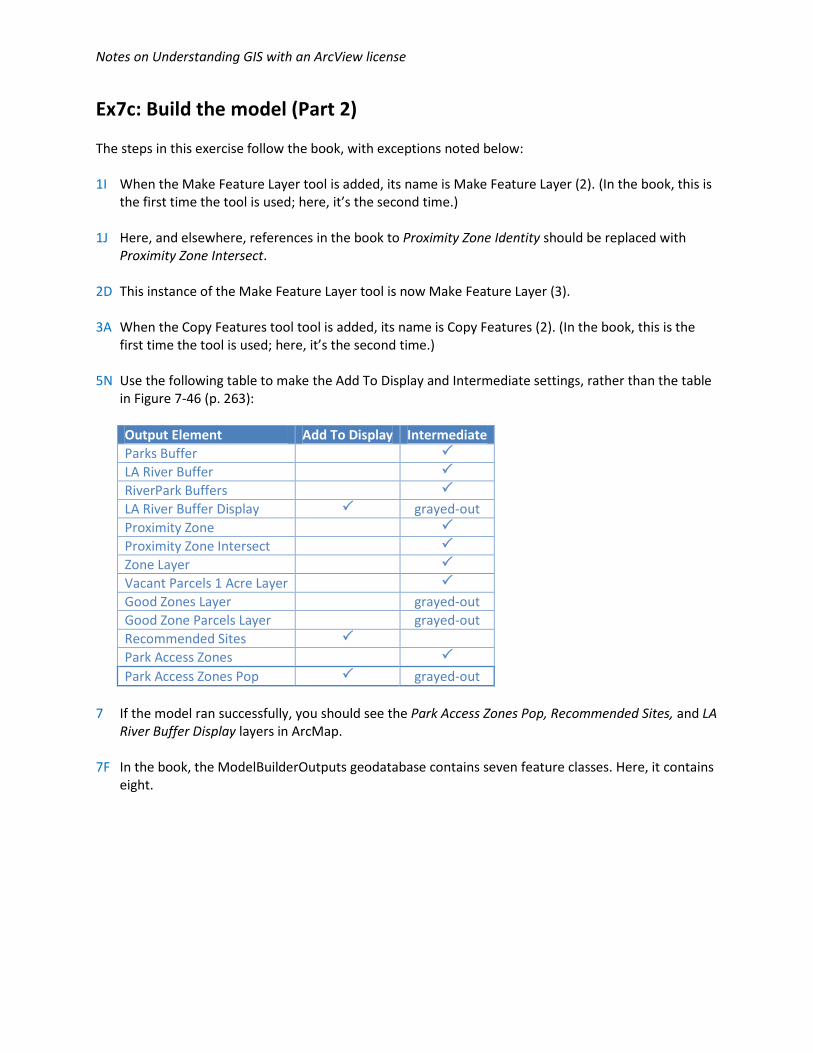
first time the tool is used; here, it’s the second time.) 5N Use the following table to make the Add To Display and Intermediate settings, rather than the table

in Figure 7-46 (p. 263):

Output Element Add To Display Intermediate

Parks Buffer

LA River Buffer

RiverPark Buffers

LA River Buffer Display grayed-out

Proximity Zone

Proximity Zone Intersect

Zone Layer

Vacant Parcels 1 Acre Layer

Good Zones Layer grayed-out

Good Zone Parcels Layer grayed-out

Recommended Sites

Park Access Zones

Park Access Zones Pop grayed-out

7 If the model ran successfully, you should see the Park Access Zones Pop, Recommended Sites, and LA

River Buffer Display layers in ArcMap. 7F In the book, the ModelBuilderOutputs geodatabase contains seven feature classes. Here, it contains

eight.


Ex7d: Run the model as a tool The steps in this exercise follow the book, with the exceptions noted below: 3G Right-click the Make Feature Layer (3) tool, connected to the Vacant Parcels input… 4D One of the output feature classes is called LARiverBufferDisplay, not LARiverBuffer. 5B In the Model window, right-click the LA River Buffer Display output data element and choose Model

Parameter. Note: the change to Step 5B is crucial. Making this element the model parameter is how we sidestep the difficulty described above in Ex7b, Step 4. The relevant part of the model looks like this:

6B Change the LA RiverBufferDisplay feature class name to LARiverBufferDisplay2. 6H LARiverBuffer2 should be LARiverBufferDisplay2.

Ex7e: Document the model The steps in this exercise follow the book, with one exception: 3I In the third bullet point, the label should be added to the Intersect tool.

Ex8a: Create the main map This exercise works as written, but remember that the positions of Sites 2 and 3 are reversed (as described above at the end of Ex6d).


Ex8b: Place inset maps and graphs


Step 4: Label the site Step 5: as is Step 6: Set label placement properties Step 7: as is Step 8: as is Step 9: as is

Step 4: Label the site In the book, Steps 4A through 4D describe turning on the Maplex extension and setting it as the label engine. For users with an ArcView-only license, turning on the Maplex extension will generate an error message that the extension isn’t licensed. In this step and throughout the remaining exercises, we’ll use the standard label engine instead. Skip Steps 4A through 4D, then do Steps 4E through 4L as written in the book. Continue as follows: 4M Click OK on the Label Expression dialog box. 4N Click Apply on the Layer Properties dialog box. Keep the dialog box open, and move it away from the

Site 1 data frame, if necessary. The label text doesn’t stack (as it would in Maplex), but runs across the feature boundary. 4O In the Other Options area of the Labels tab, click Placement Properties. 4P In the Placement Properties dialog box, on the Placement tab, click the “Try horizontal first, then

straight” option. Click OK on both open dialog boxes. Now the label is oriented along the long axis of the feature and doesn’t touch the feature outline.

4Q On the Layout toolbar, click the Zoom to 100% button. 4R On the Layout toolbar, click the Zoom Whole Page button. 4S On the map, make sure the Site 1 data frame is selected. 4T Drag the data frame to the lower right corner of the map. Step 6: Set label placement properties Skip this step.

The label before and after Step 4P.


Ex8c: Place inset maps and graphs

Step 1: Add and symbolize cities Step 2: as is Step 3: as is Step 4: Edit the city labels annotation group Step 5: Place highway markers Step 6: as is Step 7: as is Step 8: as is Step 9: as is Step 10: as is Step 11: as is Step 12: as is Step 13: as is Step 1: Add and symbolize cities Skip Steps 1C and 1D; otherwise, the step works as written. Note: Step 2 works as written, but the result at the end of the step (shown in Figure 8-65 on p. 318) is different because, without Maplex, the labels don’t stack automatically. We’ll address this in Step 4. Step 4: Edit the city labels annotation group 4A Add the Draw toolbar and confirm that the Select Elements tool is selected. 4B On the Layout toolbar, click the Focus Data Frame button. 4C Double-click the Santa Monica piece of annotation to select it and open its properties. 4D In the Properties dialog box, put the cursor between the words “Santa” and “Monica.” Delete the

space between them, the press the Enter key. Click OK. The text is now stacked as it would have been automatically with Maplex. 4E Drag the Santa Monica annotation away from the freeway, but keep it in the gray area that

separates Santa Monica from Los Angeles. 4F Double-click the Los Angeles annotation to select it and open its properties. 4G Stack the Los Angeles annotation as you did with Santa Monica in Step 4D. 4H Drag the Los Angeles annotation to a place near downtown (as in Figure 8-70 on p. 320). 4I Select the Florence annotation (lower right, behind the Site 1 inset map) and press the Delete key. 4J Delete any other annotation that is partially covered by an inset map (such as La Crescenta-

Montrose) or that identifies cities that aren’t important on our map. Possible examples are Pasadena, La Canada Flintridge, Ladera Heights, View Park-Windsor Hills, Westmont, Malibu.

4K Stack any remaining annotation that you think would look better on two or more lines. Possible examples are West Hollywood, Beverly Hills, East Los Angeles, Culver City, Marina del Rey.

4L Reposition these and any other pieces of annotation (such as Glendale) to suit your cartographic sense.

4M When you’re finished, click in a neutral part of the data frame (like the ocean) to unselect the last piece of annotation.


Ex8c: Place inset maps and graphs (continued)

Step 1: Add and symbolize cities Step 2: as is Step 3: as is Step 4: Edit the city labels annotation group Step 5: Place highway markers Step 6: as is Step 7: as is Step 8: as is Step 9: as is Step 10: as is Step 11: as is Step 12: as is Step 13: as is Step 5: Place highway markers Do steps 5A through 5G as written in the book, then continue as follows: 5H In the Label Manager, in the Placement Properties area, confirm that the Orientation is Horizontal.

Click Properties. 5J On the Placement tab, in the Duplicate Labels area, confirm that Remove duplicate labels is

selected. 5I Click OK on the Placement Properties dialog box and click OK on the Label Manager. We have too many highway symbols on the map. It looks like we have duplicates, but we actually don’t. Duplicates are multiple labels for the same feature. Here, our roads are composed of several connected features (like the Los Angeles River before we dissolved it in Lesson 4). Pacific Coast Highway (Highway 1) is labeled many times, but each label applies to a different feature. Open the MajorRoads attribute table if you want to confirm this. We could improve the label distribution slightly with some label placement techniques, but the best solution, given the fairly small number of symbols, is to convert the labels to annotation. 5K In the Table of Contents, right-click MajorRoads and choose Convert to Annotation. 5L In the Convert to Annotation dialog box, in the Store Annotation area, click “In the map.” 5M In the Create Annotation For area, click “Features in current extent.” 5N At the bottom, uncheck the box “Convert unplaced labels to unplaced annotation.” 5O Click Convert. 5P If necessary, put the data frame in focus. 5Q Delete superfluous highway symbols and reposition the others to suit your cartographic taste. You

can use the map on p. 333 as a guide. 5R When you’re finished, click in some neutral part of the data frame to unselect the last piece of

annotation.

Documents

Notes on Understanding GIS with an ArcView licensehelp.arcgis.com/en/ugis/pdf/UGIS with an ArcView license.pdfNotes on Understanding GIS with an ArcView license ... The Spatial Join