On the contribution of local feedback mechanisms to the ... · PDF fileAbstract Global and local feedback ... (Cloud Feedback Model Intercom-parison Project) and QUMP (Quantifying

M. J. Webb Æ C. A. Senior Æ D. M. H. Sexton

W. J. Ingram Æ K. D. Williams Æ M. A. Ringer

B. J. McAvaney Æ R. Colman Æ B. J. SodenR. Gudgel Æ T. Knutson Æ S. Emori Æ T. Ogura

Y. Tsushima Æ N. Andronova Æ B. Li Æ I. Musat

S. Bony Æ K. E. Taylor

On the contribution of local feedback mechanisms to the range of climatesensitivity in two GCM ensembles

Received: 1 April 2005 / Accepted: 7 December 2005 / Published online: 4 February 2006� Springer-Verlag 2006

Abstract Global and local feedback analysis techniqueshave been applied to two ensembles of mixed layerequilibrium CO2 doubling climate change experiments,from the CFMIP (Cloud Feedback Model Intercom-parison Project) and QUMP (Quantifying Uncertaintyin Model Predictions) projects. Neither of these newensembles shows evidence of a statistically significantchange in the ensemble mean or variance in global meanclimate sensitivity when compared with the results fromthe mixed layer models quoted in the Third AssessmentReport of the IPCC. Global mean feedback analysis ofthese two ensembles confirms the large contributionmade by inter-model differences in cloud feedbacks tothose in climate sensitivity in earlier studies; net cloudfeedbacks are responsible for 66% of the inter-modelvariance in the total feedback in the CFMIP ensembleand 85% in the QUMP ensemble. The ensemble meanglobal feedback components are all statistically indis-tinguishable between the two ensembles, except for the

clear-sky shortwave feedback which is stronger in theCFMIP ensemble. While ensemble variances of theshortwave cloud feedback and both clear-sky feedbackterms are larger in CFMIP, there is considerable overlapin the cloud feedback ranges; QUMP spans 80% ormore of the CFMIP ranges in longwave and shortwavecloud feedback. We introduce a local cloud feedbackclassification system which distinguishes different typesof cloud feedbacks on the basis of the relative strengthsof their longwave and shortwave components, andinterpret these in terms of responses of different cloudtypes diagnosed by the International Satellite CloudClimatology Project simulator. In the CFMIP ensemble,areas where low-top cloud changes constitute the largestcloud response are responsible for 59% of the contri-bution from cloud feedback to the variance in the totalfeedback. A similar figure is found for the QUMPensemble. Areas of positive low cloud feedback (asso-ciated with reductions in low level cloud amount)

M. J. Webb (&) Æ C. A. Senior Æ D. M. H. SextonW. J. Ingram Æ K. D. Williams Æ M. A. RingerHadley Centre for Climate Prediction and Research,Met Office, FitzRoy Road, Exeter, EX1 3PB UKE-mail: [email protected].: +44-1392-884515Fax: +44-1392-885681

B. J. McAvaney Æ R. ColmanBureau of Meteorology Research Centre (BMRC),Melbourne, Australia

B. J. SodenRosenstiel School for Marine and Atmospheric Science,University of Miami, Miami, FL, USA

R. Gudgel Æ T. KnutsonGeophysical Fluid Dynamics Laboratory (GFDL),Princeton, NJ, USA

S. Emori Æ T. OguraNational Institute for Environmental Studies (NIES),Tsukuba, Japan

Y. TsushimaFrontier Research Center for Global Change (FRCGC),Japan Agency for Marine–Earth Science and Technology,Kanagawa, Japan

N. AndronovaDepartment of Atmospheric,Oceanic and Space Sciences,University of Michigan,Ann Arbor, MI, USA

B. LiDepartment of Atmospheric Sciences,University of Illinois at Urbana–Champaign (UIUC),Urbana, IL, USA

I. Musat Æ S.BonyInstitut Pierre Simon Laplace (IPSL),Paris, France

K. E. TaylorProgram for Climate Model Diagnosis and Intercomparison(PCMDI), Livermore, CA, USA

Climate Dynamics (2006) 27: 17–38DOI 10.1007/s00382-006-0111-2

contribute most to this figure in the CFMIP ensemble,while areas of negative cloud feedback (associated withincreases in low level cloud amount and optical thick-ness) contribute most in QUMP. Classes associated withhigh-top cloud feedbacks are responsible for 33 and20% of the cloud feedback contribution in CFMIP andQUMP, respectively, while classes where no particularcloud type stands out are responsible for 8 and 21%.

1 Introduction

Estimates of the equilibrium near-surface warmingresulting from a doubling of CO2 relative to pre-indus-trial levels (often referred to as the climate sensitivity)vary among comprehensive general circulation modelsby several degrees. The Third Assessment Report (TAR)of the Intergovernmental Panel on Climate Change(IPCC; Cubasch et al. 2001) reported the range in cli-mate sensitivity from mixed layer ocean experimentswith contemporary climate models to be 2.0–5.1 K (seetheir Table 9.4, p 560).

Cess et al. (1990, 1996), Le Treut and Li (1991),Senior and Mitchell (1993), Le Treut and McAvaney(2000), Colman (2003) and others have concluded thatdifferences in cloud feedback make a large contributionto differences in climate sensitivity in GCMs. However,few of these intercomparisons have gone beyond globalor zonal mean feedback analysis, and the lack of con-sistent methods or detailed cloud diagnostics in modelshas made it difficult to compare modelled cloudresponses in a quantitative manner, meaning that thereasons for the differences in cloud response remainunclear. A number of recent developments howeverwarrant a re-visit of the issue.

There have been significant advances in methodsused to analyse and understand model feedbacks inrelation to each other and to satellite observations.Yu et al. (1996) developed an approach for detailedand quantitative comparisons of clouds in climatemodels with observations from the InternationalSatellite Cloud Climatology Project (ISCCP; Rossowand Schiffer 1999) which mimics the satellite view fromspace (along with certain ISCCP retrieval assumptions),yielding diagnostics that can be quantitatively com-pared with the observational retrievals of cloudamount, cloud top pressure and cloud optical thick-ness. Klein and Jakob (1999) and Webb et al. (2001)developed the ‘ISCCP simulator’, an implementation ofthis approach which can be run within models andwhich has been used in a number of studies (e.g. Tse-lioudis et al. 2000; Zhang et al. 2005; Williams et al.(2005b). Other studies (some of which use the ISCCPsimulator) have developed compositing techniques torelate present day variations in clouds and/or radiativefluxes to variations in thermodynamic and dynamical

variables in the models (Bony et al. 2004; Williamset al. 2003, 2005a, b; Bony and Dufresne 2005; M.C.Wyant et al., submitted). Studies of local feedbacks inindividual climate models have also emerged; Colman(2002) applied methods derived from Wetherald andManabe (1988; the so-called partial radiative pertur-bation (PRP) approach) to the Bureau of MeteorologyResearch Centre (BMRC) model, while a local analysisof feedbacks in the Canadian Climate Model (Boer andYu 2003) separated the effects of clouds and clear-skyeffects using a measure of cloud feedback based oncloud radiative forcing method of Cess and Potter(1988). These developments in cloud diagnosis andfeedback analysis techniques are now being appliedacross a range of models as part of the Cloud Feed-back Model Intercomparison Project (CFMIP; McAv-aney and Le Treut 2003; http://www.cfmip.net).CFMIP is a World Climate Research Programme(WCRP)/Working Group on Coupled Modelling(WGCM) endorsed project which aims to perform asystematic intercomparison of cloud feedbacks in cli-mate models and to evaluate aspects of their perfor-mance that are relevant to uncertainty in thosefeedbacks. The CFMIP experimental protocol requiresparticipants to include the ISCCP simulator.

The so-called perturbed physics ensembles have ex-plored the dependence of climate sensitivity of a singlemixed-layer climate model on perturbations in modelparameters. Murphy et al. (2004) report a 5–95% rangeof 1.9–5.3 K, estimated statistically by linearly com-bining the responses of single parameter perturbationsin 53 versions of HadSM3 in the first ensemble fromthe Quantifying Uncertainties in Model Predictionsproject (QUMP). Stainforth et al. (2005) analysed agrand ensemble in which 6 of the 29 QUMP parame-ters were perturbed in combination. A second QUMPensemble is now available which perturbs 29 parame-ters in combination in 128 ensemble members, with acomprehensive set of diagnostics including the ISCCPsimulator (see Sect. 2 for details). The ranges in climatesensitivity in both QUMP ensembles come close toencompassing the equivalent range from the mixedlayer models reported in the TAR, but previous studieshave not established what feedback processes contrib-ute most to this range, and whether or not these are inany way similar to those found in multi-modelensembles.

Drawing on these developments, we identify the localfeedbacks which contribute most to the inter-modeldifferences in climate sensitivity in the CFMIP andQUMP ensembles, and relate these to the responses indifferent cloud types (e.g. low and high top). We alsoquantify the extent to which the ranges of variousfeedbacks overlap in the two ensembles. We consider thedirect GCM results only, and do not attempt a formalquantification of the uncertainty in climate sensitivity orindividual climate feedbacks in the probabilistic senseused by Murphy et al. (2004).

18 Webb et al.: On the contribution of local feedback mechanisms

2 Model descriptions and experimental design

Each of the CFMIP and QUMP experiments was car-ried out with a mixed layer ‘slab’ ocean model coupledto an atmospheric GCM. In each case the steady-stateclimate was simulated for a ‘control’ concentration ofCO2 and for a doubled concentration.

A brief description of the CFMIP ensemble follows.The UIUC model is described in Yang et al. (2000) andAndronova et al. (1999). Its atmospheric resolution isN36/L24 and it has prognostic equations for cloudliquid water and ice. The BMRC model is described inColman et al. (2001). Its atmospheric resolution is T47/L17 and it has prognostic equations for cloud liquidwater and ice (Rotstayn 1997). The GFDL AM2 ‘slabmodel‘ used in this study incorporates an atmosphericmodel very similar, though not identical, to the AM2atmospheric model described in GFDL GAMDT (2004)and uses atmospheric and sea ice components verysimilar those in the CM2.0 coupled climate modeldescribed in Delworth et al. (2006). Atmospheric reso-lution is N72/L24, and it has prognostic equations forcloud liquid water and ice. HadSM3 is a version of theHadley Centre climate model and is described by Popeet al. (2000) and Williams et al. (2001a, b). Atmosphericresolution is N48/L19, and the model has prognosticequations for total water (vapour plus liquid/ice) andliquid/ice water temperature. Cloud water/ice and cloudfraction are diagnosed using a symmetric probabilitydensity function for subgrid total water variations(Smith 1990). HadSM4 is a development version ofHadSM3, described in Webb et al. (2001). Atmosphericresolution is N48/L38, and this model has a prognosticequation for cloud ice (Wilson and Ballard 1999), whilewarm clouds are as in Smith (1990), with modificationsto allow cloud to partly fill a model layer in the vertical.HadGSM1 is the mixed layer version of HadGEM1, thefirst of a new generation of Hadley Centre climatemodels (Martin et al. 2005; Johns et al. 2006). Atmo-spheric resolution is N96/L38, and while there arechanges to many areas of the atmospheric physics anddynamics, the treatment of clouds is similar to HadSM4.The Institut Pierre Simon Laplace (IPSL) model isdescribed in Hourdin et al. (2006). The atmosphericresolution is N48/L19, and the cloud parametrisation isbased on Le Treut and Li (1991). Cloud cover is pre-dicted through a statistical cloud scheme that uses a(skewed) generalised log-normal distribution to describethe subgrid-scale variability of total water. In convectiveareas the cloud scheme is coupled to the cumulus con-vection scheme after Bony and Emanuel (2001). The slabmodel version submitted to CFMIP uses climatologicalsea ice. Two model versions of the T42/L20 MIROC3.2model have been submitted to CFMIP from the CCSR/NIES/FRCGC group in Japan (K-1 model developers2004). The cloud parametrisation is based on Le Treutand Li (1991). The ‘lower-sensitivity’ version (MIROClow) is exactly the same as the ‘medium-resolution’

version of this model submitted to the IPCC FourthAssessment Report archive and described in the abovereference. The ‘higher-sensitivity’ version (MIROC high)is the same as the above except for the following twopoints in the treatment of clouds: (1) the temperaturerange for the existence of mixed phase (liquid+ice)cloud is �25 to �5�C in the higher-sensitivity version,while it is �15 to 0�C in the lower-sensitivity version; (2)when cloud ice melts, it is converted to cloud water inthe higher-sensitivity version, while it is converted torain in the lower-sensitivity version. For a fullerdescription of the two versions, see T. Ogura et al.(submitted). Note that the sea ice scheme employed inthe mixed layer model is a thermodynamic scheme, whilethe version run in the coupled version of this model ismore sophisticated.

The second QUMP ensemble is made up of 128 ver-sions of HadSM3, where a selection of 29 uncertainparameters were perturbed in combination; i.e. eachensemble member was run with multiple parameterperturbations (MPPs). The parameters used were thesame as those in the first QUMP ensemble (Murphyet al. 2004), in which only one parameter was perturbedin each ensemble member (denoted as SPP for singleparameter perturbation). The parameters were selectedfrom the major components of atmospheric and surfacephysics in the GCM, namely large scale cloud, convec-tion, radiation, boundary layer, dynamics, land surfaceprocesses and sea ice, in order to sample uncertainties inall the major surface and atmospheric processes in themodel. The MPPs were chosen to cover a range of cli-mate sensitivities while maximising, as far as possible,coverage of parameter space and model skill for a givenclimate sensitivity. Model skill is defined in this case asthe ability to reproduce time-averaged present day cli-mate according to the climate prediction index (CPI)introduced in Murphy et al. (2004). The MPPs for thesecond ensemble were generated using the followingprocedure. The size of the ensemble was chosen to be128 members, on the basis of the computing resourcesavailable. Based entirely on information contained in theSPP ensemble, an earlier version of the linear predictionmethod of Murphy et al. (2004) was used to predict theclimate sensitivities and CPI values associated with 3.6million possible MPPs generated by random samplingfrom (assumed) uniform prior distributions for eachparameter within its expert-specified limits. These pos-sible perturbations were then split into 64 equi-probablebins in climate sensitivity, and the 20 runs with the bestpredicted CPI from each bin were then selected. Fromthis 1,280 member set of MPPs, the combination withthe highest predicted skill was selected first, and thesecond was chosen to be the combination that was thefurthest away from the first in parameter space. Sub-sequent MPPs were selected such that they were in turnthe farthest from all previously selected MPPs, with theadded constraint that no more than 2 could be selectedfrom any one bin, ensuring the selection of 128 MPPs intotal. Full slab ocean experiments including calibration,

Webb et al.: On the contribution of local feedback mechanisms 19

control and equilibrium CO2 doubling components werethen run for each of the 128 MPPs, with the addition ofan interactive sulphur cycle as in Williams et al. (2001a).Sexton et al. (2004) provide additional detail on thedesign of the MPP ensemble.

In the CFMIP models, various methods were used toestimate the radiative forcing due to a doubling of CO2.The values reported here are estimates at the tropopausewith some allowance for stratospheric adjustment,except where stated otherwise below. The estimates forthe Hadley Centre and CCSR/NIES/FRCGC modelversions use the method of Tett et al. (2002). The GFDLmodel estimate uses the method of Hansen et al. (2002)diagnosing the net forcing at the surface. The BMRCmodel uses a method based on that of Colman et al.(2001) at the top of the atmosphere, while the IPSLmodel uses the method of Joshi et al. (2003). The UIUCgroup calculate an instantaneous forcing only, diag-nosed at the tropopause. This value is used unadjusted,although reducing the forcing by 15% (a typical

stratospheric adjustment) does not substantially affectthe results presented below. For all of the QUMP modelversions, the same value of CO2 forcing is assumed(3.74 Wm�2) based on the unperturbed version of themodel, as in Murphy et al. (2004).

3 Analysis of global means

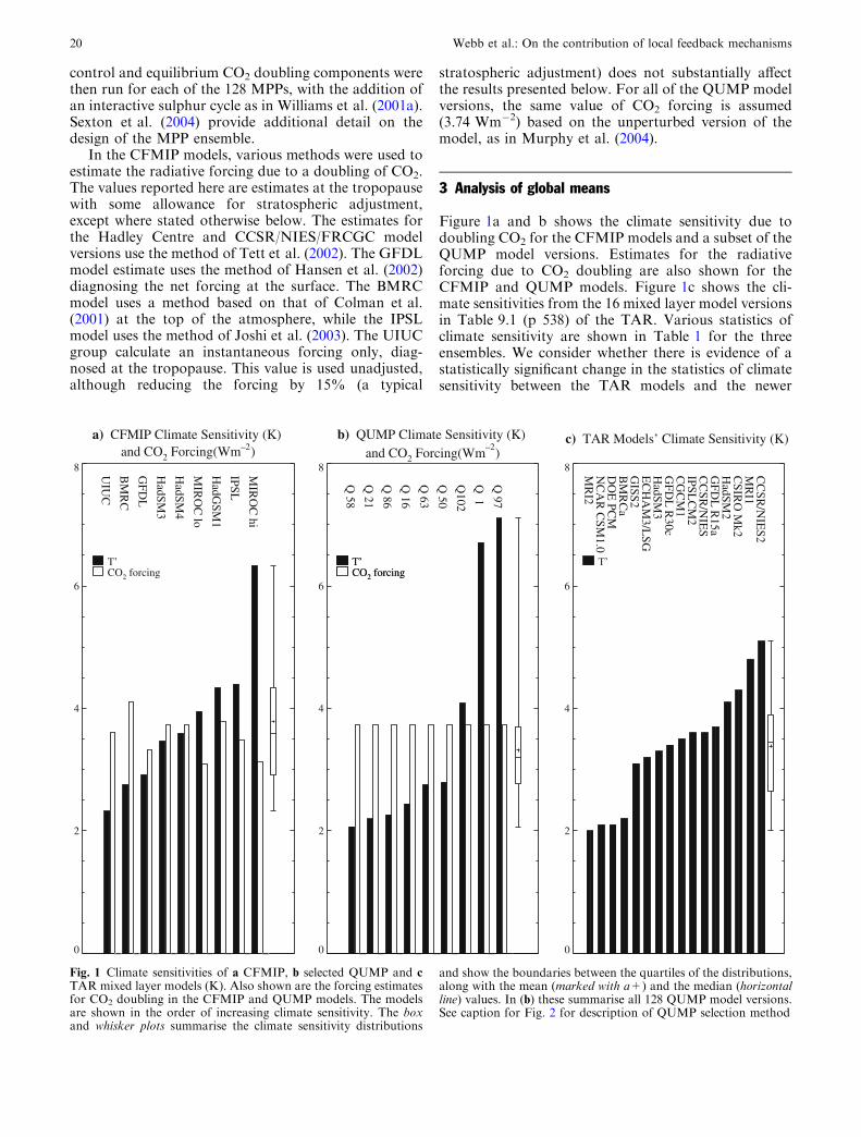
Figure 1a and b shows the climate sensitivity due todoubling CO2 for the CFMIP models and a subset of theQUMP model versions. Estimates for the radiativeforcing due to CO2 doubling are also shown for theCFMIP and QUMP models. Figure 1c shows the cli-mate sensitivities from the 16 mixed layer model versionsin Table 9.1 (p 538) of the TAR. Various statistics ofclimate sensitivity are shown in Table 1 for the threeensembles. We consider whether there is evidence of astatistically significant change in the statistics of climatesensitivity between the TAR models and the newer

a) CFMIP Climate Sensitivity (K) and CO2 Forcing(Wm–2)

0

2

4

6

8

UIU

C

BM

RC

GFD

L

HadSM

3

HadSM

4

MIR

OC

lo

HadG

SM1

IPSL

MIR

OC

hi

T’CO2 forcing

b) QUMP Climate Sensitivity (K) and CO2 Forcing(Wm–2)

0

2

4

6

8

Q 58

Q 21

Q 86

Q 16

Q 63

Q 50

Q102

Q 1

Q 97

T’CO2 forcing T’CO2 forcing

c) TAR Models’ Climate Sensitivity (K)

0

2

4

6

8

MR

I2 N

CA

R C

SM1.0

DO

E PC

M B

MR

Ca

GISS2

EC

HA

M3/L

SG H

adSM3

GFD

L R

30c C

GC

M1

IPSLC

M2

CC

SR/N

IES

GFD

L R

15a H

adSM2

CSIR

O M

k2 M

RI1

CC

SR/N

IES2

T’

Fig. 1 Climate sensitivities of a CFMIP, b selected QUMP and cTAR mixed layer models (K). Also shown are the forcing estimatesfor CO2 doubling in the CFMIP and QUMP models. The modelsare shown in the order of increasing climate sensitivity. The boxand whisker plots summarise the climate sensitivity distributions

and show the boundaries between the quartiles of the distributions,along with the mean (marked with a+) and the median (horizontalline) values. In (b) these summarise all 128 QUMP model versions.See caption for Fig. 2 for description of QUMP selection method


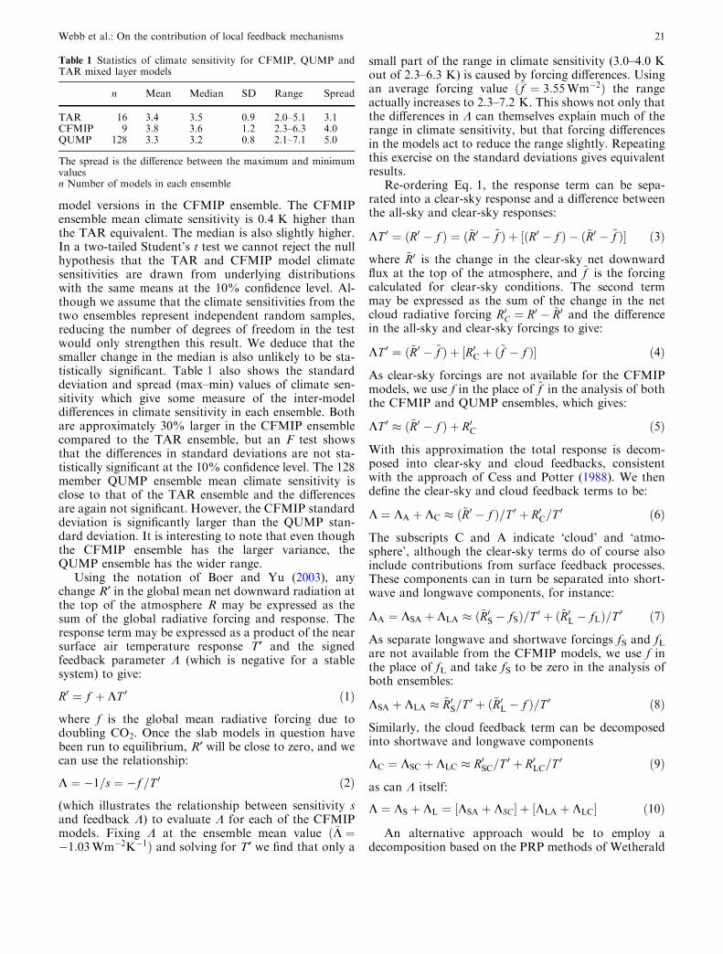
model versions in the CFMIP ensemble. The CFMIPensemble mean climate sensitivity is 0.4 K higher thanthe TAR equivalent. The median is also slightly higher.In a two-tailed Student’s t test we cannot reject the nullhypothesis that the TAR and CFMIP model climatesensitivities are drawn from underlying distributionswith the same means at the 10% confidence level. Al-though we assume that the climate sensitivities from thetwo ensembles represent independent random samples,reducing the number of degrees of freedom in the testwould only strengthen this result. We deduce that thesmaller change in the median is also unlikely to be sta-tistically significant. Table 1 also shows the standarddeviation and spread (max–min) values of climate sen-sitivity which give some measure of the inter-modeldifferences in climate sensitivity in each ensemble. Bothare approximately 30% larger in the CFMIP ensemblecompared to the TAR ensemble, but an F test showsthat the differences in standard deviations are not sta-tistically significant at the 10% confidence level. The 128member QUMP ensemble mean climate sensitivity isclose to that of the TAR ensemble and the differencesare again not significant. However, the CFMIP standarddeviation is significantly larger than the QUMP stan-dard deviation. It is interesting to note that even thoughthe CFMIP ensemble has the larger variance, theQUMP ensemble has the wider range.

Using the notation of Boer and Yu (2003), anychange R¢ in the global mean net downward radiation atthe top of the atmosphere R may be expressed as thesum of the global radiative forcing and response. Theresponse term may be expressed as a product of the nearsurface air temperature response T¢ and the signedfeedback parameter K (which is negative for a stablesystem) to give:

R0 ¼ f þ KT 0 ð1Þ

where f is the global mean radiative forcing due todoubling CO2. Once the slab models in question havebeen run to equilibrium, R¢ will be close to zero, and wecan use the relationship:

K ¼ �1=s ¼ �f =T 0 ð2Þ

(which illustrates the relationship between sensitivity sand feedback K) to evaluate K for each of the CFMIPmodels. Fixing K at the ensemble mean value ð�K ¼�1:03Wm�2K�1Þ and solving for T¢ we find that only a

small part of the range in climate sensitivity (3.0–4.0 Kout of 2.3–6.3 K) is caused by forcing differences. Usingan average forcing value ð�f ¼ 3:55Wm�2Þ the rangeactually increases to 2.3–7.2 K. This shows not only thatthe differences in K can themselves explain much of therange in climate sensitivity, but that forcing differencesin the models act to reduce the range slightly. Repeatingthis exercise on the standard deviations gives equivalentresults.

Re-ordering Eq. 1, the response term can be sepa-rated into a clear-sky response and a difference betweenthe all-sky and clear-sky responses:

KT 0 ¼ ðR0 � f Þ ¼ ð~R0 � ~f Þ þ ½ðR0 � f Þ � ð~R0 � ~f Þ� ð3Þ

where ~R0 is the change in the clear-sky net downwardflux at the top of the atmosphere, and ~f is the forcingcalculated for clear-sky conditions. The second termmay be expressed as the sum of the change in the netcloud radiative forcing R0C ¼ R0 � ~R0 and the differencein the all-sky and clear-sky forcings to give:

KT 0 ¼ ð~R0 � ~f Þ þ ½R0C þ ð~f � f Þ� ð4Þ

As clear-sky forcings are not available for the CFMIPmodels, we use f in the place of ~f in the analysis of boththe CFMIP and QUMP ensembles, which gives:

KT 0 � ð~R0 � f Þ þ R0C ð5Þ

With this approximation the total response is decom-posed into clear-sky and cloud feedbacks, consistentwith the approach of Cess and Potter (1988). We thendefine the clear-sky and cloud feedback terms to be:

K ¼ KA þ KC � ð~R0 � f Þ=T 0 þ R0C=T 0 ð6Þ

The subscripts C and A indicate ‘cloud’ and ‘atmo-sphere’, although the clear-sky terms do of course alsoinclude contributions from surface feedback processes.These components can in turn be separated into short-wave and longwave components, for instance:

KA ¼ KSA þ KLA � ð~R0S � fSÞ=T 0 þ ð~R0L � fLÞ=T 0 ð7Þ

As separate longwave and shortwave forcings fS and fLare not available from the CFMIP models, we use f inthe place of fL and take fS to be zero in the analysis ofboth ensembles:

KSA þ KLA � ~R0S=T 0 þ ð~R0L � f Þ=T 0 ð8Þ

Similarly, the cloud feedback term can be decomposedinto shortwave and longwave components

KC ¼ KSC þ KLC � R0SC=T 0 þ R0LC=T 0 ð9Þ

as can K itself:

K ¼ KS þ KL ¼ ½KSA þ KSC� þ ½KLA þ KLC� ð10Þ

An alternative approach would be to employ adecomposition based on the PRP methods of Wetherald

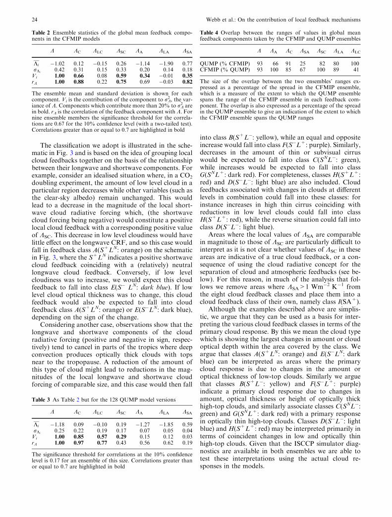
Table 1 Statistics of climate sensitivity for CFMIP, QUMP andTAR mixed layer models

n Mean Median SD Range Spread

TAR 16 3.4 3.5 0.9 2.0–5.1 3.1CFMIP 9 3.8 3.6 1.2 2.3–6.3 4.0QUMP 128 3.3 3.2 0.8 2.1–7.1 5.0

The spread is the difference between the maximum and minimumvaluesn Number of models in each ensemble


and Manabe (1988) and Colman (2002) which give asomewhat cleaner separation of forcing and feedbackcomponents, avoiding the so-called cloud masking effectwhich (when the cloud forcing method is used) leads toan overestimate of the strength of clear-sky feedbackterms and an underestimate of the strength of cloudterms (Zhang et al. 1994; Colman 2003; Soden et al.2004). This approach however requires suitable diag-nostics which are not currently available for a widerange of models. In this study therefore, the term ‘cloudfeedback’ will (unless stated otherwise) refer to thatcomponent of the feedback measured by the change inthe cloud radiative forcing.

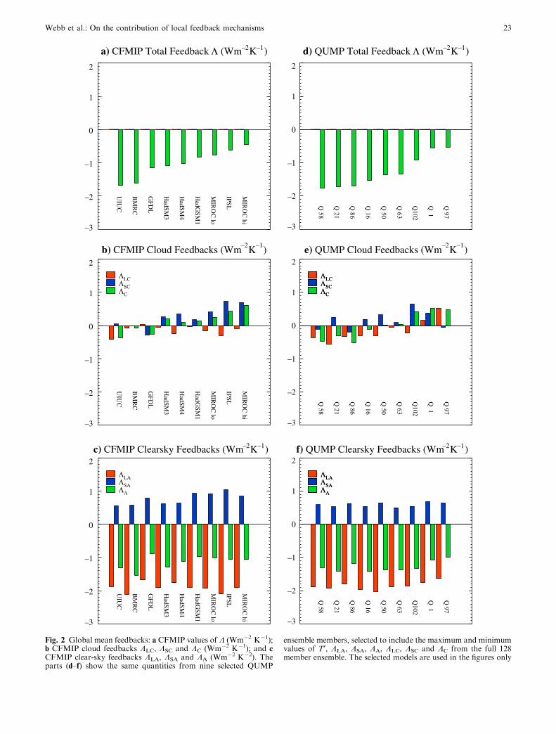
Table 2 presents statistics based on those of Boer andYu (2003), but applied to inter-model differences inglobal mean feedback components Ki taken across theCFMIP ensemble, rather than across the spatial struc-ture of the feedback components in a single model. Foreach component Ki we show the ensemble mean �Ki; theensemble sample standard deviation rKi ; and Vi, thefractional contribution of the global mean feedbackcomponent Ki to rK

2 (the ensemble variance of K),defined as

Vi ¼X

k¼1;n

Kþk Kþikr2

Kðn� 1Þ ð11Þ

where (Kik+, k=1,n) are the deviations of the individual

models from the ensemble mean. The contributions sumto unity, but may take negative as well as positive values.The table also shows correlations of Ki with K.

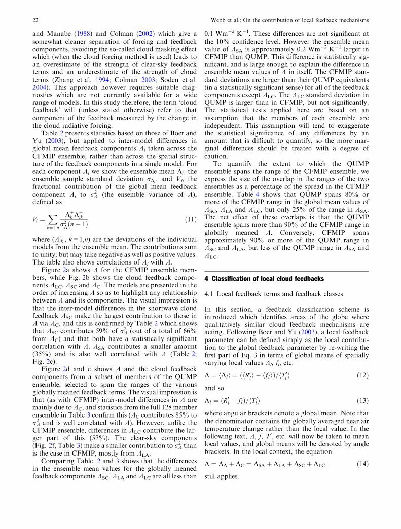
Figure 2a shows K for the CFMIP ensemble mem-bers, while Fig. 2b shows the cloud feedback compo-nents KLC, KSC and KC. The models are presented in theorder of increasing K so as to highlight any relationshipbetween K and its components. The visual impression isthat the inter-model differences in the shortwave cloudfeedback KSC make the largest contribution to those inK via KC, and this is confirmed by Table 2 which showsthat KSC contributes 59% of rK

2 (out of a total of 66%from KC) and that both have a statistically significantcorrelation with K. KSA contributes a smaller amount(35%) and is also well correlated with K (Table 2;Fig. 2c).

Figure 2d and e shows K and the cloud feedbackcomponents from a subset of members of the QUMPensemble, selected to span the ranges of the variousglobally meaned feedback terms. The visual impression isthat (as with CFMIP) inter-model differences in K aremainly due to KC, and statistics from the full 128 memberensemble in Table 3 confirm this (KC contributes 85% torK2 and is well correlated with K). However, unlike the

CFMIP ensemble, differences in KLC contribute the lar-ger part of this (57%). The clear-sky components(Fig. 2f, Table 3) make a smaller contribution to rK

2 thanis the case in CFMIP, mostly from KLA.

Comparing Table. 2 and 3 shows that the differencesin the ensemble mean values for the globally meanedfeedback components KSC, KLA and KLC are all less than

0.1 Wm�2 K�1. These differences are not significant atthe 10% confidence level. However the ensemble meanvalue of KSA is approximately 0.2 Wm�2 K�1 larger inCFMIP than QUMP. This difference is statistically sig-nificant, and is large enough to explain the difference inensemble mean values of K in itself. The CFMIP stan-dard deviations are larger than their QUMP equivalents(in a statistically significant sense) for all of the feedbackcomponents except KLC. The KLC standard deviation inQUMP is larger than in CFMIP, but not significantly.The statistical tests applied here are based on anassumption that the members of each ensemble areindependent. This assumption will tend to exaggeratethe statistical significance of any differences by anamount that is difficult to quantify, so the more mar-ginal differences should be treated with a degree ofcaution.

To quantify the extent to which the QUMPensemble spans the range of the CFMIP ensemble, weexpress the size of the overlap in the ranges of the twoensembles as a percentage of the spread in the CFMIPensemble. Table 4 shows that QUMP spans 80% ormore of the CFMIP range in the global mean values ofKSC, KLA and KLC, but only 25% of the range in KSA.The net effect of these overlaps is that the QUMPensemble spans more than 90% of the CFMIP range inglobally meaned K. Conversely, CFMIP spansapproximately 90% or more of the QUMP range inKSC and KLA, but less of the QUMP range in KSA andKLC.

4 Classification of local cloud feedbacks

4.1 Local feedback terms and feedback classes

In this section, a feedback classification scheme isintroduced which identifies areas of the globe wherequalitatively similar cloud feedback mechanisms areacting. Following Boer and Yu (2003), a local feedbackparameter can be defined simply as the local contribu-tion to the global feedback parameter by re-writing thefirst part of Eq. 3 in terms of global means of spatiallyvarying local values Kl, fl, etc.

K ¼ hKli ¼ ðhR0li � hfliÞ=hT 0l i ð12Þ

and so

Kl ¼ ðR0l � flÞ=hT 0l i ð13Þ

where angular brackets denote a global mean. Note thatthe denominator contains the globally averaged near airtemperature change rather than the local value. In thefollowing text, K, f, T¢, etc. will now be taken to meanlocal values, and global means will be denoted by anglebrackets. In the local context, the equation

K ¼ KA þ KC ¼ KSA þ KLA þ KSC þ KLC ð14Þ

still applies.


a) CFMIP Total Feedback Λ (Wm–2K–1)

–3

–2

–1

0

1

2

UIU

C

BM

RC

GFD

L

HadSM

3

HadSM

4

HadG

SM1

MIR

OC

lo

IPSL

MIR

OC

hi

b) CFMIP Cloud Feedbacks (Wm–2K–1)

–3

–2

–1

0

1

2

UIU

C

BM

RC

GFD

L

HadSM

3

HadSM

4

HadG

SM1

MIR

OC

lo

IPSL

MIR

OC

hi

ΛLCΛSCΛC

c) CFMIP Clearsky Feedbacks (Wm–2K–1)

–3

–2

–1

0

1

2

UIU

C

BM

RC

GFD

L

HadSM

3

HadSM

4

HadG

SM1

MIR

OC

lo

IPSL

MIR

OC

hi

ΛLAΛSAΛA

d) QUMP Total Feedback Λ (Wm–2K–1)

–3

–2

–1

0

1

2

Q 58

Q 21

Q 86

Q 16

Q 50

Q 63

Q102

Q 1

Q 97

e) QUMP Cloud Feedbacks (Wm–2K–1)

–3

–2

–1

0

1

2

Q 58

Q 21

Q 86

Q 16

Q 50

Q 63

Q102

Q 1

Q 97

ΛLCΛSCΛC

ΛLCΛSCΛC

f) QUMP Clearsky Feedbacks (Wm–2K–1)

–3

–2

–1

0

1

2

Q 58

Q 21

Q 86

Q 16

Q 50

Q 63

Q102

Q 1

Q 97

ΛLAΛSAΛA

ΛLAΛSAΛA

Fig. 2 Global mean feedbacks: a CFMIP values of K (Wm�2 K�1);b CFMIP cloud feedbacks KLC, KSC and KC (Wm�2 K�1); and cCFMIP clear-sky feedbacks KLA, KSA and KA (Wm�2 K�2). Theparts (d–f) show the same quantities from nine selected QUMP

ensemble members, selected to include the maximum and minimumvalues of T¢, KLA, KSA, KA, KLC, KSC and KC from the full 128member ensemble. The selected models are used in the figures only


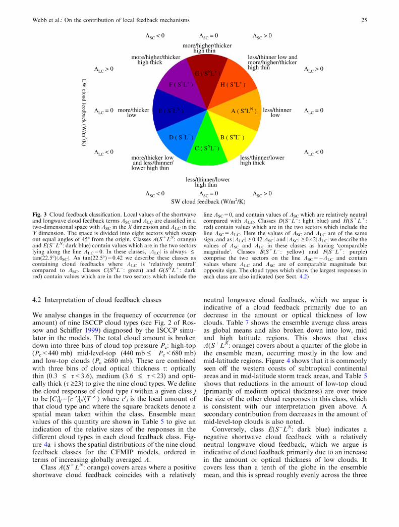
The classification we adopt is illustrated in the sche-matic in Fig. 3 and is based on the idea of grouping localcloud feedbacks together on the basis of the relationshipbetween their longwave and shortwave components. Forexample, consider an idealised situation where, in a CO2

doubling experiment, the amount of low level cloud in aparticular region decreases while other variables (such asthe clear-sky albedo) remain unchanged. This wouldlead to a decrease in the magnitude of the local short-wave cloud radiative forcing which, (the shortwavecloud forcing being negative) would constitute a positivelocal cloud feedback with a corresponding positive valueof KSC. This decrease in low level cloudiness would havelittle effect on the longwave CRF, and so this case wouldfall in feedback class A(S+LN: orange) on the schematicin Fig. 3, where the S+LN indicates a positive shortwavecloud feedback coinciding with a (relatively) neutrallongwave cloud feedback. Conversely, if low levelcloudiness was to increase, we would expect this cloudfeedback to fall into class E(S� LN: dark blue). If lowlevel cloud optical thickness was to change, this cloudfeedback would also be expected to fall into cloudfeedback class A(S+LN: orange) or E(S�LN: dark blue),depending on the sign of the change.

Considering another case, observations show that thelongwave and shortwave components of the cloudradiative forcing (positive and negative in sign, respec-tively) tend to cancel in parts of the tropics where deepconvection produces optically thick clouds with topsnear to the tropopause. A reduction of the amount ofthis type of cloud might lead to reductions in the mag-nitudes of the local longwave and shortwave cloudforcing of comparable size, and this case would then fall

into class B(S+L�: yellow), while an equal and oppositeincrease would fall into class F(S�L+: purple). Similarly,decreases in the amount of thin or subvisual cirruswould be expected to fall into class C(SNL�: green),while increases would be expected to fall into classG(SNL+: dark red). For completeness, classes H(S+L+:red) and D(S�L�: light blue) are also included. Cloudfeedbacks associated with changes in clouds at differentlevels in combination could fall into these classes: forinstance increases in high thin cirrus coinciding withreductions in low level clouds could fall into classH(S+L+: red), while the reverse situation could fall intoclass D(S�L�: light blue).

Areas where the local values of KSA are comparablein magnitude to those of KSC are particularly difficult tointerpret as it is not clear whether values of KSC in theseareas are indicative of a true cloud feedback, or a con-sequence of using the cloud radiative concept for theseparation of cloud and atmospheric feedbacks (see be-low). For this reason, in much of the analysis that fol-lows we remove areas where KSA>1 Wm�2 K�1 fromthe eight cloud feedback classes and place them into acloud feedback class of their own, namely class I(SA+).

Although the examples described above are simplis-tic, we argue that they can be used as a basis for inter-preting the various cloud feedback classes in terms of theprimary cloud response. By this we mean the cloud typewhich is showing the largest changes in amount or cloudoptical depth within the area covered by the class. Weargue that classes A(S+LN: orange) and E(S�LN: darkblue) can be interpreted as areas where the primarycloud response is due to changes in the amount oroptical thickness of low-top clouds. Similarly we arguethat classes B(S+L�: yellow) and F(S�L+: purple)indicate a primary cloud response due to changes inamount, optical thickness or height of optically thickhigh-top clouds, and similarly associate classes C(SNL�:green) and G(SNL+: dark red) with a primary responsein optically thin high-top clouds. Classes D(S�L�: lightblue) and H(S+L+: red) may be interpreted primarily interms of coincident changes in low and optically thinhigh-top clouds. Given that the ISCCP simulator diag-nostics are available in both ensembles we are able totest these interpretations using the actual cloud re-sponses in the models.

Table 2 Ensemble statistics of the global mean feedback compo-nents in the CFMIP models

K KC KLC KSC KA KLA KSA

Ki �1.02 0.12 �0.15 0.26 �1.14 �1.90 0.77rKi 0.42 0.31 0.15 0.33 0.20 0.14 0.18Vi 1.00 0.66 0.08 0.59 0.34 �0.01 0.35rK 1.00 0.88 0.22 0.75 0.69 �0.03 0.82

The ensemble mean and standard deviation is shown for eachcomponent. Vi is the contribution of the component to rK

2 , the var-iance of K. Components which contribute more than 20% to rK

2 arein bold. rK is the correlation of the feedback component with K. Fornine ensemble members the significance threshold for the correla-tions are 0.67 for the 10% confidence level (with a two-tailed test).Correlations greater than or equal to 0.7 are highlighted in bold

Table 4 Overlap between the ranges of values in global meanfeedback components taken by the CFMIP and QUMP ensembles

K KA KC KSA KSC KLA KLC

QUMP (% CFMIP) 93 66 91 25 82 80 100CFMIP (% QUMP) 93 100 85 67 100 89 41

The size of the overlap between the two ensembles’ ranges ex-pressed as a percentage of the spread in the CFMIP ensemble,which is a measure of the extent to which the QUMP ensemblespans the range of the CFMIP ensemble in each feedback com-ponent. The overlap is also expressed as a percentage of the spreadin the QUMP ensemble to give an indication of the extent to whichthe CFMIP ensemble spans the QUMP ranges

Table 3 As Table 2 but for the 128 QUMP model versions

K KC KLC KSC KA KLA KSA

Ki �1.18 0.09 �0.10 0.19 �1.27 �1.85 0.59rKi 0.25 0.22 0.19 0.17 0.07 0.05 0.04Vi 1.00 0.85 0.57 0.29 0.15 0.12 0.03rK 1.00 0.97 0.77 0.43 0.56 0.62 0.19

The significance threshold for correlations at the 10% confidencelevel is 0.17 for an ensemble of this size. Correlations greater thanor equal to 0.7 are highlighted in bold


4.2 Interpretation of cloud feedback classes

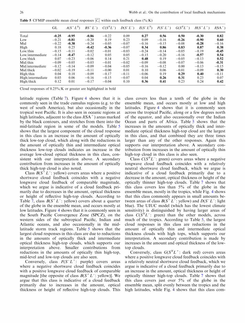
We analyse changes in the frequency of occurrence (oramount) of nine ISCCP cloud types (see Fig. 2 of Ros-sow and Schiffer 1999) diagnosed by the ISCCP simu-lator in the models. The total cloud amount is brokendown into three bins of cloud top pressure Pc: high-top(Pc<440 mb) mid-level-top (440 mb £ Pc<680 mb)and low-top clouds (Pc ‡680 mb). These are combinedwith three bins of cloud optical thickness s: opticallythin (0.3 £ s<3.6), medium (3.6 £ s<23) and opti-cally thick (s ‡23) to give the nine cloud types. We definethe cloud response of cloud type i within a given class jto be [Ci]j=[c ¢i]j/ÆT ¢ æ where c¢i is the local amount ofthat cloud type and where the square brackets denote aspatial mean taken within the class. Ensemble meanvalues of this quantity are shown in Table 5 to give anindication of the relative sizes of the responses in thedifferent cloud types in each cloud feedback class. Fig-ure 4a–i shows the spatial distributions of the nine cloudfeedback classes for the CFMIP models, ordered interms of increasing globally averaged K.

Class A(S+LN: orange) covers areas where a positiveshortwave cloud feedback coincides with a relatively

neutral longwave cloud feedback, which we argue isindicative of a cloud feedback primarily due to andecrease in the amount or optical thickness of lowclouds. Table 7 shows the ensemble average class areasas global means and also broken down into low, midand high latitude regions. This shows that classA(S+LN: orange) covers about a quarter of the globe inthe ensemble mean, occurring mostly in the low andmid-latitude regions. Figure 4 shows that it is commonlyseen off the western coasts of subtropical continentalareas and in mid-latitude storm track areas, and Table 5shows that reductions in the amount of low-top cloud(primarily of medium optical thickness) are over twicethe size of the other cloud responses in this class, whichis consistent with our interpretation given above. Asecondary contribution from decreases in the amount ofmid-level-top clouds is also noted.

Conversely, class E(S�LN: dark blue) indicates anegative shortwave cloud feedback with a relativelyneutral longwave cloud feedback, which we argue isindicative of cloud feedback primarily due to an increasein the amount or optical thickness of low clouds. Itcovers less than a tenth of the globe in the ensemblemean, and this is spread roughly evenly across the three

At 00:00Z on 0/ 0/ 0

18090S

45S

0

45N

D ( S L )

more/thicker low and less/thinner/lower high thin

E ( S LN ) more/thicker low

F ( S L+ )

more/higher/thicker high thick

C ( SNL )

less/thinner/lower high thin

G ( SNL+ )

more/higher/thicker high thin

B ( S+L )

less/thinner/lower high thick

A ( S+LN ) less/thinner low

H ( S+L+ )

less/thinner low and more/higher/thicker high thin

ΛSC < 0 ΛSC = 0 ΛSC > 0

ΛSC < 0 ΛSC = 0 ΛSC > 0SW cloud feedback (W/m2/K)

ΛLC < 0

ΛLC = 0

ΛLC > 0

ΛLC < 0

ΛLC = 0

ΛLC > 0

LW

cloud feedback (W/m

2/K)

–

–

– – –

–

Fig. 3 Cloud feedback classification. Local values of the shortwaveand longwave cloud feedback terms KSC and KLC are classified in atwo-dimensional space with KSC in the X dimension and KLC in theY dimension. The space is divided into eight sectors which sweepout equal angles of 45� from the origin. Classes A(S+LN: orange)and E(S�LN: dark blue) contain values which are in the two sectorslying along the line KLC=0. In these classes, |KLC| is always £tan(22.5�)|KSC|. As tan(22.5�)=0.42 we describe these classes ascontaining cloud feedbacks where KLC is ‘relatively neutral’compared to KSC. Classes C(SNL�: green) and G(SNL+: darkred) contain values which are in the two sectors which include the

line KSC=0, and contain values of KSC which are relatively neutralcompared with KLC. Classes D(S�L�: light blue) and H(S+L+:red) contain values which are in the two sectors which include theline KSC=KLC. Here the values of KSC and KLC are of the samesign, and as |KLC| ‡ 0.42|KSC| and |KSC| ‡ 0.42|KLC| we describe thevalues of KSC and KLC in these classes as having ‘comparablemagnitude’. Classes B(S+L�: yellow) and F(S�L+: purple)comprise the two sectors on the line KSC=�KLC and containvalues where KLC and KSC are of comparable magnitude butopposite sign. The cloud types which show the largest responses ineach class are also indicated (see Sect. 4.2)


latitude regions (Table 7). Figure 4 shows that it iscommonly seen in the trade cumulus regions (e.g. to thewest of south America), but also occasionally in thetropical west Pacific. It is also seen in oceanic regions athigh latitudes, adjacent to the class I(SA+) areas markedby the black contours, and stretches from there into themid-latitude region in some of the models. Table 5shows that the largest component of the cloud responsein this class is an increase in the amount of opticallythick low-top cloud, which along with the reductions inthe amount of optically thin and intermediate opticalthickness low-top clouds indicates an increase in theaverage low-cloud optical thickness in this class, con-sistent with our interpretation above. A secondarycontribution from increases in the amount of opticallythick high-top cloud is also noted.

Class B(S+L�: yellow) covers areas where a positiveshortwave cloud feedback coincides with a negativelongwave cloud feedback of comparable magnitude,which we argue is indicative of a cloud feedback pri-marily due to decreases in the amount, optical thicknessor height of reflective high-top clouds. According toTable 7, class B(S+L�: yellow) covers about a quarterof the globe in the ensemble mean, and occurs mostly atlow latitudes. Figure 4 shows that it is commonly seen inthe South Pacific Convergence Zone (SPCZ), on thewestern sides of the subtropical Pacific, Indian andAtlantic oceans, and also occasionally in the mid-latitude storm track regions. Table 5 shows that thelargest cloud responses in this class are due to reductionsin the amounts of optically thick and intermediateoptical thickness high-top clouds, which supports ourinterpretation above. Smaller contributions fromreductions in the amounts of optically thin high-top,mid-level and low-top clouds are also seen.

Conversely, class F(S�L+: purple) covers areaswhere a negative shortwave cloud feedback coincideswith a positive longwave cloud feedback of comparablemagnitude [the opposite of class B(S+L�: yellow)]. Weargue that this class is indicative of a cloud feedbackprimarily due to increases in the amount, opticalthickness or height of reflective high-top clouds. This

class covers less than a tenth of the globe in theensemble mean, and occurs mostly at low and highlatitudes. Figure 4 shows that it is commonly seenacross the tropical Pacific, along or a few degrees northof the equator, and also occasionally over the IndianOcean and parts of Africa. Table 5 shows that theincreases in the amounts of optically thick and inter-mediate optical thickness high-top cloud are the largestin this class, and that combined they are three timeslarger than any of the other responses. Again thissupports our interpretation above. A secondary con-tribution from increases in the amount of optically thinhigh-top cloud in this class is also seen.

Class C(SNL�: green) covers areas where a negativelongwave cloud feedback coincides with a relativelyneutral shortwave cloud feedback, which we argue isindicative of a cloud feedback primarily due to adecrease in the amount, optical thickness or height of theoptically thinner high-top clouds. Table 7 shows thatthis class covers less than 5% of the globe in theensemble mean, mostly in the tropics, while Fig. 4 showsthat this class commonly appears in small amounts be-tween areas of class B(S+L�: yellow) and D(S�L�: lightblue). The UIUC model (which has the lowest climatesensitivity) is distinguished by having larger areas ofclass C(SNL�: green) than the other models, acrossmuch of the tropics. According to Table 5, the largestcloud responses in this class are reductions in theamount of optically thin and intermediate opticalthickness clouds with high tops, which supports ourinterpretation. A secondary contribution is made byincreases in the amount and optical thickness of the low-top clouds.

Conversely, class G(SNL+: dark red) covers areaswhere a positive longwave cloud feedback coincides witha relatively neutral shortwave cloud feedback, which weargue is indicative of a cloud feedback primarily due toan increase in the amount, optical thickness or height ofoptically thinner high-top clouds. Table 7 shows thatthis class covers just over 5% of the globe in theensemble mean, split evenly between the tropics and thehigh latitudes, while Fig. 4 shows that this class com-

Table 5 CFMIP ensemble mean cloud responses ½Ci� within each feedback class (%/K)

GL A(S+LN) BS+L�) C(SNL�) D(S�L�) E(S�LN) F(S�L+) G(SNL+) H(S+L+) I(SA+)

Total -0.25 -0.95 -0.86 �0.22 0.09 0.27 0.56 0.50 -0.30 0.82Low �0.21 -0.81 �0.20 0.19 0.23 0.09 �0.16 -0.26 -0.90 0.60Mid �0.22 -0.38 �0.24 �0.05 �0.07 �0.16 �0.15 �0.08 -0.28 �0.16High 0.18 0.25 -0.42 -0.36 �0.07 0.34 0.86 0.83 0.87 0.38Low/thin �0.15 �0.11 �0.02 �0.01 �0.03 �0.24 �0.14 �0.05 �0.19 -0.45Low/intermediate �0.14 -0.47 �0.12 0.05 0.05 �0.15 �0.20 �0.16 -0.57 0.54Low/thick 0.07 �0.23 �0.06 0.14 0.21 0.48 0.19 �0.05 �0.13 0.52Mid/thin �0.09 �0.05 �0.03 �0.01 �0.02 �0.09 �0.08 �0.07 �0.06 -0.31Mid/intermediate �0.12 �0.14 �0.09 �0.04 �0.05 �0.16 �0.12 0.00 �0.13 �0.15Mid/thick �0.02 �0.19 �0.11 �0.00 0.01 0.10 0.06 �0.01 �0.09 0.30High/thin 0.04 0.18 �0.09 �0.17 �0.11 �0.06 0.19 0.29 0.40 �0.11High/intermediate 0.03 0.06 �0.16 �0.15 �0.07 0.04 0.26 0.31 0.23 0.07High/thick 0.12 0.01 �0.17 �0.04 0.10 0.36 0.41 0.23 0.24 0.42

Cloud responses of 0.25%/K or greater are highlighted in bold


UIU

C

T’ =

2.

32K

090

E18

090

W90

S

45S0

45N

90N

1

1

1

1

1

1

11

1

BM

RC

T

’ =

2.75

K

090

E18

090

W0

90S

45S0

45N

90N

11

1

1

1

1

1

GFD

L

T’ =

2.

92K

090

E18

090

W0

90S

45S0

45N

90N

1

1

1

1

1

1

11

1

Had

SM3

T’ =

3.

47K

090

E18

090

W90

S

45S0

45N

90N

1

1

1

1

1

1

1

11

11

Had

SM4

T’ =

3.

59K

090

E18

090

W90

S

45S0

45N

90N

1

1

1

1

1

11

11

Had

GSM

1 T

’ =

4.34

K

090

E18

090

W90

S

45S0

45N

90N

1

1

1

1

1

11

1

MIR

OC

T

’ =

3.95

K

090

E18

090

W0

45S0

45N

90N

1

1

1

1

11

111

1

1

IPSL

T

’ =

4.40

K

090

E18

090

W90

S

45S0

45N

90N

1

1

11

11

1

1

1

MIR

OC

hi

T’ =

6.

34K

090

E18

090

W0

45S0

45N

90N

1

1

1

11

1

1

Fig.4

SpatialdistributionofCFMIP

cloudfeedback

classes.Theareasoftheglobecovered

byeach

oftheeightcloudfeedback

classes

are

shownbyplottingtheassigned

colourofeach

class

atlocationswherethelocalfeedback

components

fallinto

thatclass.Forexample,theorangeareasshow

whereclass

A(S

+LN:orange)

behaviouris

present—

i.e.where

KSCispositivebutKLCisrelativelyneutral.Class

I(SA

+)areasare

enclosedbyblack

contours,butcolourcoded

consistentlywithwhichever

oftheeight

originalcloudfeedback

classes

thatthey

wereinitiallyplacedin


monly appears near areas of class F(S�L+: purple) inthe tropics, and over Antarctica. Table 5 showsincreases in high-top cloud amount are more than twicethe size of the mid- and low-top cloud responses, andthat this is mainly due to increases in the amount ofintermediate/thin optical thickness high-top cloud,which is consistent with our interpretation. Reductionsin the amount of low-top cloud play a secondary role.

Class H(S+L+: red) covers areas where a positivelongwave cloud feedback coincides with a positiveshortwave cloud feedback of comparable magnitude. Itis not clear that changes in a single cloud type could beresponsible for a cloud feedback of this type. However,as class H(S+L+: red) sits between classes A(S+LN:orange) and G(SNL+: dark red) in the cloud feedbackphase space, we argue that this class is indicative of acombination of the cloud responses seen in these twoclasses—i.e. reductions in low-top cloud amount and/oroptical thickness combined with increases in theamount, optical thickness or height of optically thinhigh-top clouds. Table 7 shows that this class covers justunder 5% of the globe in the ensemble mean, half in thetropics and a quarter in each of the mid-latitude andhigh latitude regions, while Fig. 4 shows it to commonlyappear between class A(S+LN: orange) and H(S+L+:red) areas. According to Table 5, the largest cloudresponses are due to an increase in the amount of (pri-marily optically thin) high-top cloud and a reduction inlow-top cloud amount (primarily of intermediate opticalthickness), which supports our interpretation.

Conversely, class D(S�L�: light blue) covers areaswhere a negative longwave cloud feedback coincides

with a negative shortwave cloud feedback of comparablemagnitude. As with class H(S+L+: red) above, we arguethat this is indicative a cloud feedback due to a combi-nation of the cloud feedback behaviour from the adja-cent classes [primarily reductions in amount or opticalthickness of the optically thinner high-top clouds as inclass C(SNL�: green) and increases in low-top cloudamount and/or optical thickness as in class E(S�LN:dark blue)]. Table 7 shows that this class covers less than5% of the globe in the ensemble mean, two-thirds in thetropics and one-third in the mid-latitude region, andFig. 4 shows that it appears mainly between areas ofclass C(SNL�: green) and E(S�LN: dark blue). Table 5shows the largest cloud responses in this class indicate anincrease in the amount and optical thickness of low-topclouds, and a reduction in the optically thin and inter-mediate optical thickness high-top cloud amounts,which is consistent with the interpretation above. Thereis also a smaller increase in the optically thick high-topcloud, as in class E(S�LN: dark blue).

Finally we turn to class I(SA+), which we have de-fined to contain all cloud feedbacks which coincide witha positive clear-sky shortwave feedback whereKSA>1 Wm�2 K�1. This threshold was chosen experi-mentally to select areas (mostly at high latitudes) wherechanges in sea-ice and snow mean that they reflect lesssunlight in the warmer climate. This class covers about15% of the globe in the ensemble mean, the vastmajority of which is in the high latitude region, andFig. 4 shows that in these areas the CFMIP modelsshow mostly class E(S�LN: dark blue) and F(S�L+:purple)-like behaviour, indicating negative values of

Table 6 As Table 5 but for the QUMP ensemble

GL A(S+LN) B(S+L�) C(SNL�) D(S�L�) E(S�LN) F(S�L+) G(SNL+) H(S+L+) I(SA+)

Total �0.19 �1.02 �0.95 �0.27 0.14 0.61 0.87 0.53 �0.18 0.58Low �0.14 �0.84 �0.09 0.40 0.55 0.49 �0.18 �0.34 �0.85 0.30Mid �0.27 �0.35 �0.23 �0.15 �0.18 �0.26 �0.16 �0.13 �0.23 �0.39High 0.23 0.17 �0.63 �0.51 �0.23 0.38 1.21 0.99 0.90 0.66Low/thin �0.20 �0.16 �0.07 �0.03 �0.04 �0.21 �0.13 �0.13 �0.20 �0.58Low/intermediate �0.05 �0.50 �0.09 0.16 0.29 0.29 �0.08 �0.16 �0.52 0.46Low/thick 0.11 �0.18 0.07 0.26 0.30 0.41 0.03 �0.05 �0.14 0.42Mid/thin �0.11 �0.09 �0.05 �0.04 �0.06 �0.15 �0.10 �0.12 �0.07 �0.22Mid/intermediate �0.12 �0.10 �0.09 �0.06 �0.06 �0.10 �0.08 0.01 �0.09 �0.32Mid/thick �0.05 �0.16 �0.10 �0.05 �0.06 �0.01 0.02 �0.02 �0.07 0.15High/thin 0.07 0.18 �0.21 �0.27 �0.19 �0.05 0.46 0.45 0.44 0.00High/intermediate 0.07 0.06 �0.07 �0.04 0.01 0.09 0.25 0.29 0.17 0.11High/thick 0.09 �0.07 �0.35 �0.20 �0.05 0.34 0.51 0.26 0.29 0.55

Table 7 CFMIP class area statistics by region

Class area A(S+LN) B(S+L�) C(SNL�) D(S�L�) E(S�LN) F(S�L+) G(SNL+) H(S+L+) I(SA+)

Global 0.25 0.25 0.05 0.03 0.07 0.08 0.06 0.04 0.1630�N–30�S 0.13 0.18 0.04 0.02 0.03 0.04 0.03 0.03 0.0030�–50� N/S 0.10 0.07 0.01 0.01 0.02 0.01 0.01 0.01 0.0350�–90� N/S 0.01 0.00 0.00 0.00 0.03 0.02 0.03 0.01 0.13

The ensemble means of the fractional area covered by each class are shown for the whole globe, and for low latitude (30�N–30�S), mid-latitude (30�N–50�N, 30�S–50�S) and high latitude (50�N–90�N, 50�S–90�S) regions. The fractions of the globe covered by each region oflatitude are 50, 26 and 24%, respectively


Q58

T

’ =

2.07

K

090

E18

090

W90

S

45S0

45N

90N

1

11

1

1

11

1 1

Q21

T

’ =

2.19

K

090

E18

090

W90

S

45S0

45N

90N

11

1

1

1

Q86

T

’ =

2.26

K

090

E18

090

W90

S

45S0

45N

90N

1

1

1

1

1

1

1

1 1

11

11

1

Q16

T

’ =

2.44

K

090

E18

090

W90

S

45S0

45N

90N

1

1

1

1

1

111

1

1

1

1

Q63

T

’ =

2.75

K

090

E18

090

W90

S

45S0

45N

90N

1

1

1

1

11

11

11

11

11

1

Q50

T

’ =

2.79

K

090

E18

090

W90

S

45S0

45N

90N

1

1

1

1

1

11

1

11

1

1

1

1

1

11

Q10

2 T

’ =

4.09

K

090

E18

090

W90

S

45S0

45N

90N

1

1

1

1

1

1 11

1

Q01

T

’ =

6.71

K

090

E18

090

W90

S

45S0

45N

90N

1

1

1

1

11

1

11

1

11

Q97

T

’ =

7.11

K

090

E18

090

W90

S

45S0

45N

90N

1

1

1

1

11

1

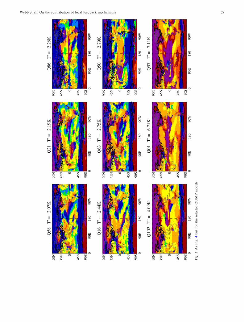
Fig.5AsFig.4butfortheselected

QUMPmodels


KSC. However, this alone is not evidence that the cloudsin these areas are necessarily showing increases in theiramount or cloud optical thickness. This is because, evenwith no change in cloud properties, a reduction in clear-sky albedo can give a negative value of KSC. This effectcan be illustrated using a simple idealised model, wherewe consider the effects of surface reflection and scatter-ing of shortwave radiation by clouds only. For instance,if:

RS ¼ �S½ac þ ð1� acÞas� ð15Þ

and

~RS ¼ �Sas ð16Þ

where S is the incoming solar radiation, as is the surfacealbedo and ac represents the cloud albedo, then theshortwave cloud forcing

RSC ¼ RS � ~RS ¼ �S½ac þ ð1� acÞas � as�¼ �Sacð1� asÞ

In the case where as decreases while ac remains un-changed, the magnitude of the shortwave cloud radiativeforcing will increase (which will give a positive value ofKSA and a negative value of KSC). This is an example ofthe cloud masking effect discussed by Colman (2003)and Soden et al. (2004). It is because of this difficulty ininterpreting the meaning of KSC in areas of clear-skyshortwave feedback that we place areas whereKSA>1 Wm�2 K�1 into a separate class. We can how-ever interpret the cloud feedbacks in this class using ourunderstanding of the cloud feedbacks in other classes.Table 5 shows that the largest ensemble mean cloudresponses in this class are for the low-top clouds, withincreases in the amounts of optically thick and inter-mediate optical thickness low-top cloud and reductionsin the amount of optically thin low-top clouds. Thesechanges indicate that the primary cause of the cloudfeedback in this class is an increase in the amount andoptical thickness of low-top clouds which is consistentwith the cloud response in class E(S�LN: dark blue)where a truly negative shortwave cloud feedback isoperating. Increases in the amount of high-top opticallythick cloud play a secondary role, which is also consis-tent with class E(S�LN: dark blue). From this we con-clude that the ensemble mean cloud responses in classI(SA+) are fully consistent with the presence of a trulynegative shortwave cloud feedback.

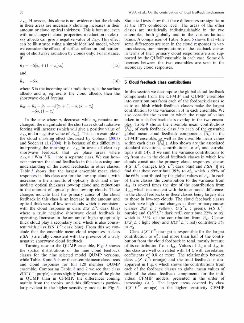
Turning now to the QUMP ensemble, Fig. 5 showsthe spatial distributions of the nine cloud feedbackclasses for the nine selected model QUMP versions,while Table. 8 and 6 show the ensemble mean class areasand cloud responses for full 128 member QUMPensemble. Comparing Table. 8 and 7 we see that classF(S�L+: purple) covers slightly larger areas of the globein QUMP than in CFMIP, the differences comingmainly from the tropics, and this difference is particu-larly evident in the higher sensitivity models in Fig. 5.

Statistical tests show that these differences are significantat the 10% confidence level. The areas of the otherclasses are statistically indistinguishable in the twoensembles, both globally and in the various latitudebands. A comparison of Table. 6 and 5 shows that whilesome differences are seen in the cloud responses in var-ious classes, our interpretations of the feedback classesin terms of their primary cloud responses are also sup-ported by the QUMP ensemble in each case. Some dif-ferences between the two ensembles are seen in thesecondary cloud responses.

5 Cloud feedback class contributions

In this section we decompose the global cloud feedbackcomponents from the CFMIP and QUMP ensemblesinto contributions from each of the feedback classes soas to establish which feedback classes make the largestcontribution to the variance in K in each ensemble. Wealso consider the extent to which the range of valuestaken in each feedback class overlap in the two ensem-bles. Table 9 shows the ensemble mean contributionshKiij of each feedback class j to each of the ensembleglobal mean cloud feedback components hKii in theCFMIP ensemble, as well as the ensemble mean valueswithin each class ð½Ki�jÞ: Also shown are the associatedstandard deviations, contributions to rK

2 and correla-tions with ÆKæ. If we sum the variance contributions torK2 from KC in the cloud feedback classes in which low

clouds constitute the primary cloud responses [classesA(S+LN: orange), E(S�LN: dark blue) and I(SA+)] wefind that these contribute 39% to rK

2 , which is 59% ofthe 66% contributed by the global values of KC. In eachof these classes the contribution to the variance fromKSC is several times the size of the contribution fromKLC, which is consistent with the inter-model differencesin the cloud feedbacks in these classes being largely dueto those in low-top clouds. The cloud feedback classeswhich have high cloud changes as their primary causes[classes B(S+L�: yellow), C(SNL�: green), F(S�L+:purple) and G(SNL+: dark red)] contribute 22% to rK

2 ,which is 33% of the contribution from KC. ClassesD(S�L�: light blue) and H(S+L+: red) contribute 5%to rK

2 .Class A(S+LN: orange) is responsible for the largest

contribution to rK2 , and more than half of the contri-

bution from the cloud feedback in total, mostly becauseof its contribution from KSC. Values of KC and KSC inthis class are well correlated with ÆK æ, with correlationcoefficients of 0.8 or more. The relationship betweenclass A(S+LN: orange) and the total feedback is alsoapparent in Fig. 6 which shows the contributions fromeach of the feedback classes to global mean values ofeach of the cloud feedback components for the indi-vidual CFMIP models, presented in the order ofincreasing ÆK æ. The larger areas covered by classA(S+LN: orange) in the higher sensitivity CFMIP


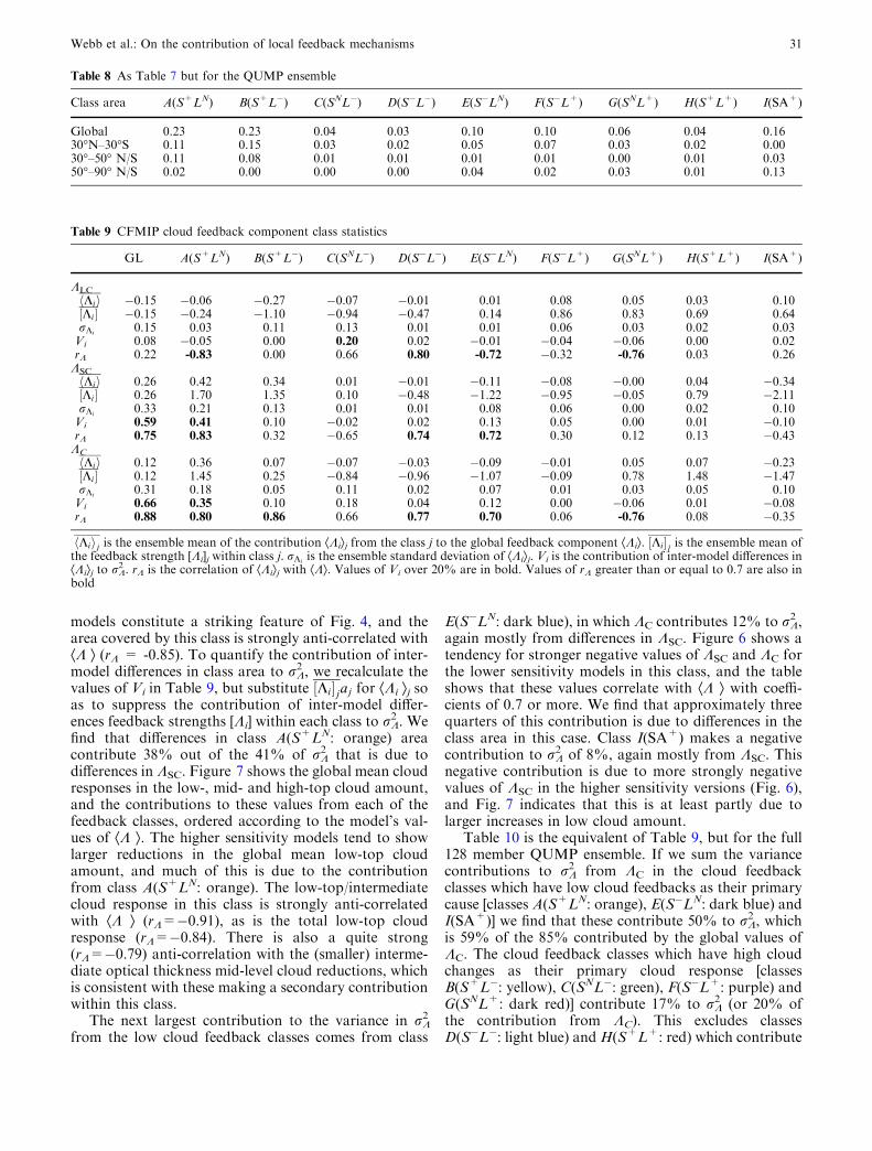
models constitute a striking feature of Fig. 4, and thearea covered by this class is strongly anti-correlated withÆK æ (rK = -0.85). To quantify the contribution of inter-model differences in class area to rK

2 , we recalculate thevalues of Vi in Table 9, but substitute ½Ki�jaj for ÆKi æj soas to suppress the contribution of inter-model differ-ences feedback strengths [Ki] within each class to rK

2 . Wefind that differences in class A(S+LN: orange) areacontribute 38% out of the 41% of rK

2 that is due todifferences in KSC. Figure 7 shows the global mean cloudresponses in the low-, mid- and high-top cloud amount,and the contributions to these values from each of thefeedback classes, ordered according to the model’s val-ues of ÆK æ. The higher sensitivity models tend to showlarger reductions in the global mean low-top cloudamount, and much of this is due to the contributionfrom class A(S+LN: orange). The low-top/intermediatecloud response in this class is strongly anti-correlatedwith ÆK æ (rK=�0.91), as is the total low-top cloudresponse (rK=�0.84). There is also a quite strong(rK=�0.79) anti-correlation with the (smaller) interme-diate optical thickness mid-level cloud reductions, whichis consistent with these making a secondary contributionwithin this class.

The next largest contribution to the variance in rK2

from the low cloud feedback classes comes from class

E(S�LN: dark blue), in which KC contributes 12% to rK2 ,

again mostly from differences in KSC. Figure 6 shows atendency for stronger negative values of KSC and KC forthe lower sensitivity models in this class, and the tableshows that these values correlate with ÆK æ with coeffi-cients of 0.7 or more. We find that approximately threequarters of this contribution is due to differences in theclass area in this case. Class I(SA+) makes a negativecontribution to rK

2 of 8%, again mostly from KSC. Thisnegative contribution is due to more strongly negativevalues of KSC in the higher sensitivity versions (Fig. 6),and Fig. 7 indicates that this is at least partly due tolarger increases in low cloud amount.

Table 10 is the equivalent of Table 9, but for the full128 member QUMP ensemble. If we sum the variancecontributions to rK

2 from KC in the cloud feedbackclasses which have low cloud feedbacks as their primarycause [classes A(S+LN: orange), E(S�LN: dark blue) andI(SA+)] we find that these contribute 50% to rK

2 , whichis 59% of the 85% contributed by the global values ofKC. The cloud feedback classes which have high cloudchanges as their primary cloud response [classesB(S+L�: yellow), C(SNL�: green), F(S�L+: purple) andG(SNL+: dark red)] contribute 17% to rK

2 (or 20% ofthe contribution from KC). This excludes classesD(S�L�: light blue) and H(S+L+: red) which contribute

Table 9 CFMIP cloud feedback component class statistics


KLC

hKii �0.15 �0.06 �0.27 �0.07 �0.01 0.01 0.08 0.05 0.03 0.10½Ki� �0.15 �0.24 �1.10 �0.94 �0.47 0.14 0.86 0.83 0.69 0.64rKi 0.15 0.03 0.11 0.13 0.01 0.01 0.06 0.03 0.02 0.03Vi 0.08 �0.05 0.00 0.20 0.02 �0.01 �0.04 �0.06 0.00 0.02rK 0.22 -0.83 0.00 0.66 0.80 -0.72 �0.32 -0.76 0.03 0.26KSC

hKii 0.26 0.42 0.34 0.01 �0.01 �0.11 �0.08 �0.00 0.04 �0.34½Ki� 0.26 1.70 1.35 0.10 �0.48 �1.22 �0.95 �0.05 0.79 �2.11rKi 0.33 0.21 0.13 0.01 0.01 0.08 0.06 0.00 0.02 0.10Vi 0.59 0.41 0.10 �0.02 0.02 0.13 0.05 0.00 0.01 �0.10rK 0.75 0.83 0.32 �0.65 0.74 0.72 0.30 0.12 0.13 �0.43KC

hKii 0.12 0.36 0.07 �0.07 �0.03 �0.09 �0.01 0.05 0.07 �0.23½Ki� 0.12 1.45 0.25 �0.84 �0.96 �1.07 �0.09 0.78 1.48 �1.47rKi 0.31 0.18 0.05 0.11 0.02 0.07 0.01 0.03 0.05 0.10Vi 0.66 0.35 0.10 0.18 0.04 0.12 0.00 �0.06 0.01 �0.08rK 0.88 0.80 0.86 0.66 0.77 0.70 0.06 -0.76 0.08 �0.35

hKiij is the ensemble mean of the contribution ÆKiæj from the class j to the global feedback component ÆKiæ. ½Ki�j is the ensemble mean ofthe feedback strength [Ki]j within class j. rKi is the ensemble standard deviation of ÆKiæj. Vi is the contribution of inter-model differences inÆKiæj to rK

2 . rK is the correlation of ÆKiæj with ÆKæ. Values of Vi over 20% are in bold. Values of rK greater than or equal to 0.7 are also inbold


Class area A(S+LN) B(S+L�) C(SNL�) D(S�L�) E(S�LN) F(S�L+) G(SNL+) H(S+L+) I(SA+)

Global 0.23 0.23 0.04 0.03 0.10 0.10 0.06 0.04 0.1630�N–30�S 0.11 0.15 0.03 0.02 0.05 0.07 0.03 0.02 0.0030�–50� N/S 0.11 0.08 0.01 0.01 0.01 0.01 0.00 0.01 0.0350�–90� N/S 0.02 0.00 0.00 0.00 0.04 0.02 0.03 0.01 0.13


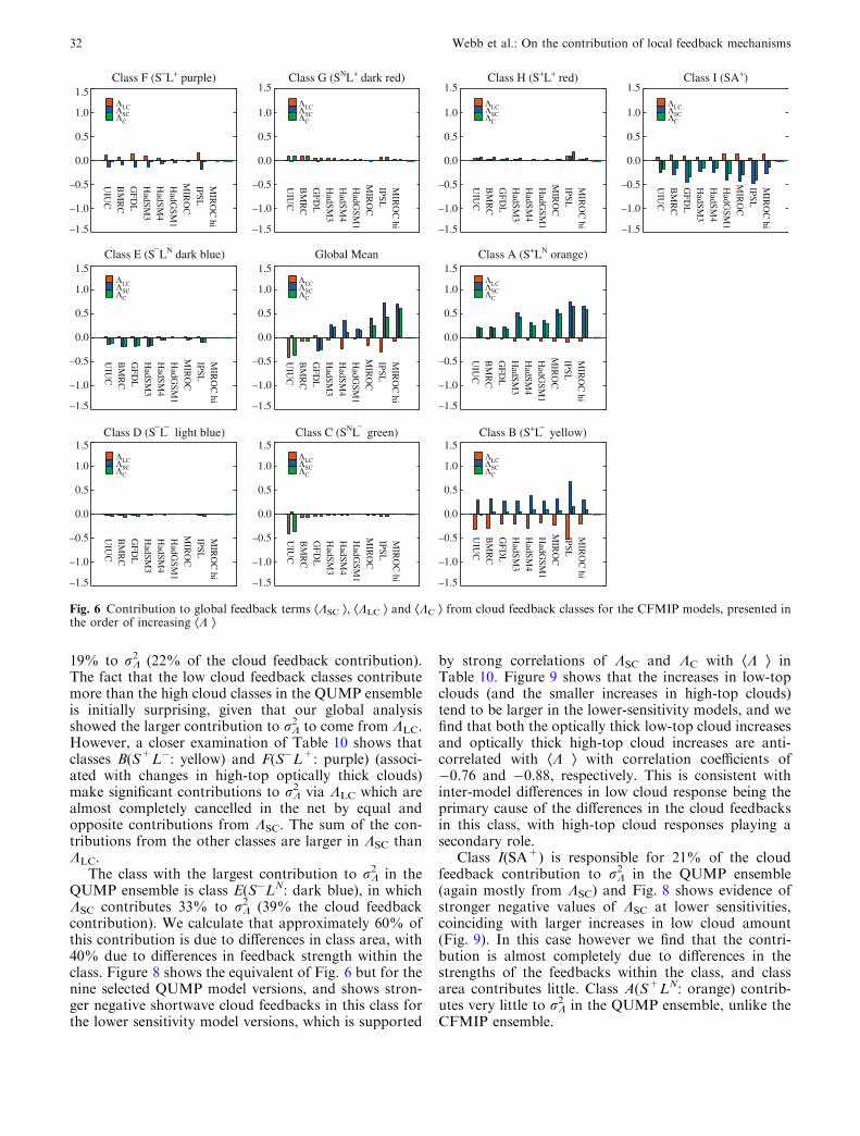
19% to rK2 (22% of the cloud feedback contribution).

The fact that the low cloud feedback classes contributemore than the high cloud classes in the QUMP ensembleis initially surprising, given that our global analysisshowed the larger contribution to rK

2 to come from KLC.However, a closer examination of Table 10 shows thatclasses B(S+L�: yellow) and F(S�L+: purple) (associ-ated with changes in high-top optically thick clouds)make significant contributions to rK

2 via KLC which arealmost completely cancelled in the net by equal andopposite contributions from KSC. The sum of the con-tributions from the other classes are larger in KSC thanKLC.

The class with the largest contribution to rK2 in the

QUMP ensemble is class E(S�LN: dark blue), in whichKSC contributes 33% to rK

2 (39% the cloud feedbackcontribution). We calculate that approximately 60% ofthis contribution is due to differences in class area, with40% due to differences in feedback strength within theclass. Figure 8 shows the equivalent of Fig. 6 but for thenine selected QUMP model versions, and shows stron-ger negative shortwave cloud feedbacks in this class forthe lower sensitivity model versions, which is supported

by strong correlations of KSC and KC with ÆK æ inTable 10. Figure 9 shows that the increases in low-topclouds (and the smaller increases in high-top clouds)tend to be larger in the lower-sensitivity models, and wefind that both the optically thick low-top cloud increasesand optically thick high-top cloud increases are anti-correlated with ÆK æ with correlation coefficients of�0.76 and �0.88, respectively. This is consistent withinter-model differences in low cloud response being theprimary cause of the differences in the cloud feedbacksin this class, with high-top cloud responses playing asecondary role.

Class I(SA+) is responsible for 21% of the cloudfeedback contribution to rK

2 in the QUMP ensemble(again mostly from KSC) and Fig. 8 shows evidence ofstronger negative values of KSC at lower sensitivities,coinciding with larger increases in low cloud amount(Fig. 9). In this case however we find that the contri-bution is almost completely due to differences in thestrengths of the feedbacks within the class, and classarea contributes little. Class A(S+LN: orange) contrib-utes very little to rK

2 in the QUMP ensemble, unlike theCFMIP ensemble.

Class F (S L+–

–

– – – –

purple)

–1.5

–1.0

–0.5

0.0

0.5

1.0

1.5

UIU

C B

MR

C G

FDL

HadSM

3 H

adSM4

HadG

SM1

MIR

OC

IPSL M

IRO

C hi

ΛLCΛSCΛC

Class E (S LN dark blue)

–1.5

–1.0

–0.5

0.0

0.5

1.0

1.5ΛLCΛSCΛC

Class D (S L light blue)

–1.5

–1.0

–0.5

0.0

0.5

1.0

1.5ΛLCΛSCΛC

Class G (SNL+ dark red)

–1.5

–1.0

–0.5

0.0

0.5

1.0

1.5

UIU

C B

MR

C G

FDL

HadSM

3 H

adSM4

HadG

SM1

MIR

OC

IPSL M

IRO

C hi

ΛLCΛSCΛC

Global Mean

–1.5

–1.0

–0.5

0.0

0.5

1.0

1.5ΛLCΛSCΛC

Class C (SNL green)

–1.5

–1.0

–0.5

0.0

0.5

1.0

1.5ΛLCΛSCΛC

Class H (S+L+ red)

–1.5

–1.0

–0.5

0.0

0.5

1.0

1.5

UIU

C B

MR

C G

FDL

HadSM

3 H

adSM4

HadG

SM1

MIR

OC

IPSL M

IRO

C hi

UIU

C B

MR

C G

FDL

HadSM

3 H

adSM4

HadG

SM1

MIR

OC

IPSL M

IRO

C hi

UIU

C B

MR

C G

FDL

HadSM

3 H

adSM4

HadG

SM1

MIR

OC

IPSL M

IRO

C hi

UIU

C B

MR

C G

FDL

HadSM

3 H

adSM4

HadG

SM1

MIR

OC

IPSL M

IRO

C hi

UIU

C B

MR

C G

FDL

HadSM

3 H

adSM4

HadG

SM1

MIR

OC

IPSL M

IRO

C hi

UIU

C B

MR

C G

FDL

HadSM

3 H

adSM4

HadG

SM1

MIR

OC

IPSL M

IRO

C hi

UIU

C B

MR

C G

FDL

HadSM

3 H

adSM4

HadG

SM1

MIR

OC

IPSL M

IRO

C hi

UIU

C B

MR

C G

FDL

HadSM

3 H

adSM4

HadG

SM1

MIR

OC

IPSL M

IRO

C hi

ΛLCΛSCΛC

Class A (S+LN orange)

–1.5

–1.0

–0.5

0.0

0.5

1.0

1.5ΛLCΛSCΛC

Class B (S+L yellow)

–1.5

–1.0

–0.5

0.0

0.5

1.0

1.5ΛLCΛSCΛC

Class I (SA+)

–1.5

–1.0

–0.5

0.0

0.5

1.0

1.5

ΛLCΛSCΛC

Fig. 6 Contribution to global feedback terms ÆKSC æ, ÆKLC æ and ÆKC æ from cloud feedback classes for the CFMIP models, presented inthe order of increasing ÆK æ


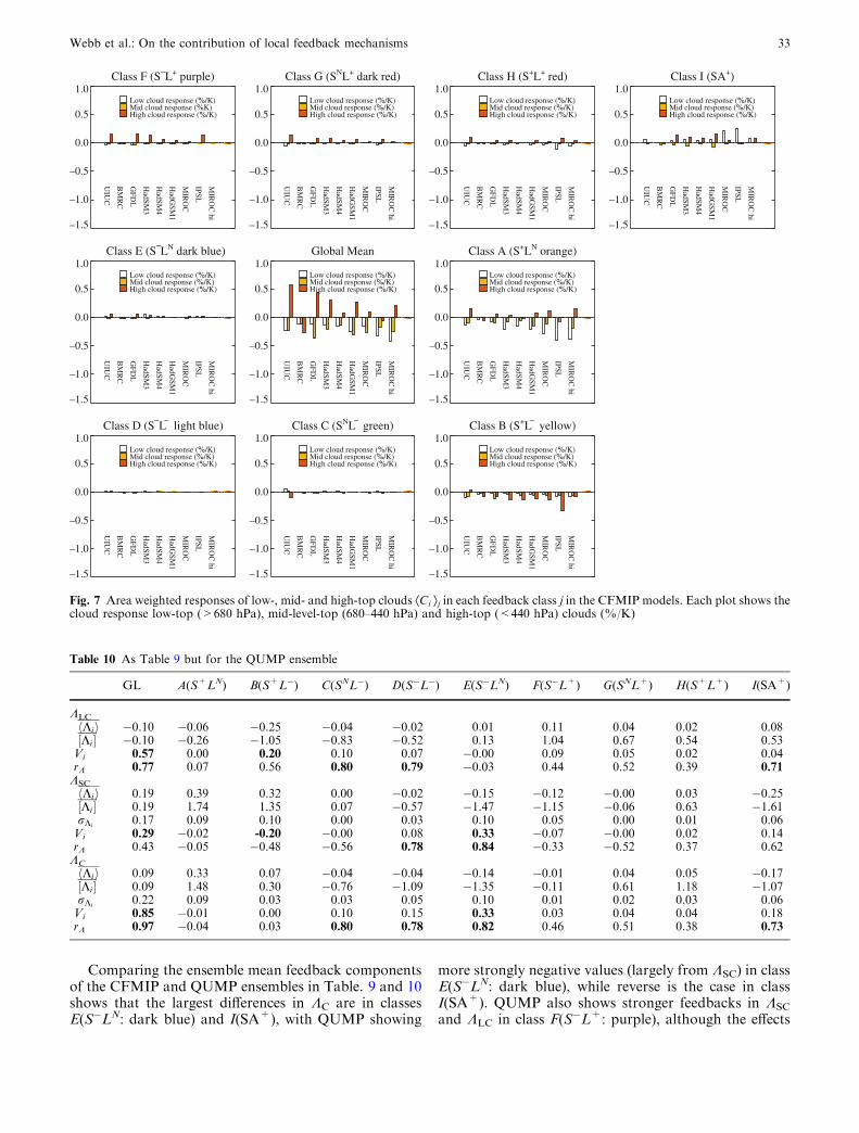
Comparing the ensemble mean feedback componentsof the CFMIP and QUMP ensembles in Table. 9 and 10shows that the largest differences in KC are in classesE(S�LN: dark blue) and I(SA+), with QUMP showing

more strongly negative values (largely from KSC) in classE(S�LN: dark blue), while reverse is the case in classI(SA+). QUMP also shows stronger feedbacks in KSC

and KLC in class F(S�L+: purple), although the effects

Class F (S L+ purple)

–1.5

–1.0

–0.5

0.0

0.5

1.0

UIU

C

BM

RC

GFD

L

HadSM

3

HadSM

4

HadG

SM1

MIR

OC

IPSL

MIR

OC

hi

Low cloud response (%/K)Mid cloud response (%K)High cloud response (%/K)


–1.5

–1.0

–0.5

0.0

0.5

1.0

UIU

C

BM

RC

GFD

L

HadSM

3

HadSM

4

HadG

SM1

MIR

OC

IPSL

MIR

OC

hi

Low cloud response (%/K)Mid cloud response (%/K)High cloud response (%/K)


–1.5

–1.0

–0.5

0.0

0.5

1.0

UIU

C

BM

RC

GFD

L

HadSM

3

HadSM

4

HadG

SM1

MIR

OC

IPSL

MIR

OC

hi



–1.5

–1.0

–0.5

0.0

0.5

1.0

UIU

C

BM

RC

GFD

L

HadSM

3

HadSM

4

HadG

SM1

MIR

OC

IPSL

MIR

OC

hi


Global Mean

–1.5

–1.0

–0.5

0.0

0.5

1.0

UIU

C

BM

RC

GFD

L

HadSM

3

HadSM

4

HadG

SM1

MIR

OC

IPSL

MIR

OC

hi


Class C (SNL green)

–1.5

–1.0

–0.5

0.0

0.5

1.0

UIU

C

BM

RC

GFD

L

HadSM

3

HadSM

4

HadG

SM1

MIR

OC

IPSL

MIR

OC

hi


Class H (S+L+ red)

–1.5

–1.0

–0.5

0.0

0.5

1.0

UIU

C

BM

RC

GFD

L

HadSM

3

HadSM

4

HadG

SM1

MIR

OC

IPSL

MIR

OC

hi



–1.5

–1.0

–0.5

0.0

0.5

1.0

UIU

C

BM

RC

GFD

L

HadSM

3

HadSM

4

HadG

SM1

MIR

OC

IPSL

MIR

OC

hi



–1.5

–1.0

–0.5

0.0

0.5

1.0

UIU

C

BM

RC

GFD

L

HadSM

3

HadSM

4

HadG

SM1

MIR

OC

IPSL

MIR

OC

hi


Class I (SA+)

–1.5

–1.0

–0.5

0.0

0.5

1.0

UIU

C

BM

RC

GFD

L

HadSM

3

HadSM

4

HadG

SM1

MIR

OC

IPSL

MIR

OC

hiLow cloud response (%/K)Mid cloud response (%/K)High cloud response (%/K)

–

–

– – – –

Fig. 7 Area weighted responses of low-, mid- and high-top clouds ÆCi æj in each feedback class j in the CFMIP models. Each plot shows thecloud response low-top (>680 hPa), mid-level-top (680–440 hPa) and high-top (<440 hPa) clouds (%/K)



KLC

hKii �0.10 �0.06 �0.25 �0.04 �0.02 0.01 0.11 0.04 0.02 0.08½Ki� �0.10 �0.26 �1.05 �0.83 �0.52 0.13 1.04 0.67 0.54 0.53Vi 0.57 0.00 0.20 0.10 0.07 �0.00 0.09 0.05 0.02 0.04rK 0.77 0.07 0.56 0.80 0.79 �0.03 0.44 0.52 0.39 0.71KSC

hKii 0.19 0.39 0.32 0.00 �0.02 �0.15 �0.12 �0.00 0.03 �0.25½Ki� 0.19 1.74 1.35 0.07 �0.57 �1.47 �1.15 �0.06 0.63 �1.61rKi 0.17 0.09 0.10 0.00 0.03 0.10 0.05 0.00 0.01 0.06Vi 0.29 �0.02 -0.20 �0.00 0.08 0.33 �0.07 �0.00 0.02 0.14rK 0.43 �0.05 �0.48 �0.56 0.78 0.84 �0.33 �0.52 0.37 0.62KC

hKii 0.09 0.33 0.07 �0.04 �0.04 �0.14 �0.01 0.04 0.05 �0.17½Ki� 0.09 1.48 0.30 �0.76 �1.09 �1.35 �0.11 0.61 1.18 �1.07rKi 0.22 0.09 0.03 0.03 0.05 0.10 0.01 0.02 0.03 0.06Vi 0.85 �0.01 0.00 0.10 0.15 0.33 0.03 0.04 0.04 0.18rK 0.97 �0.04 0.03 0.80 0.78 0.82 0.46 0.51 0.38 0.73


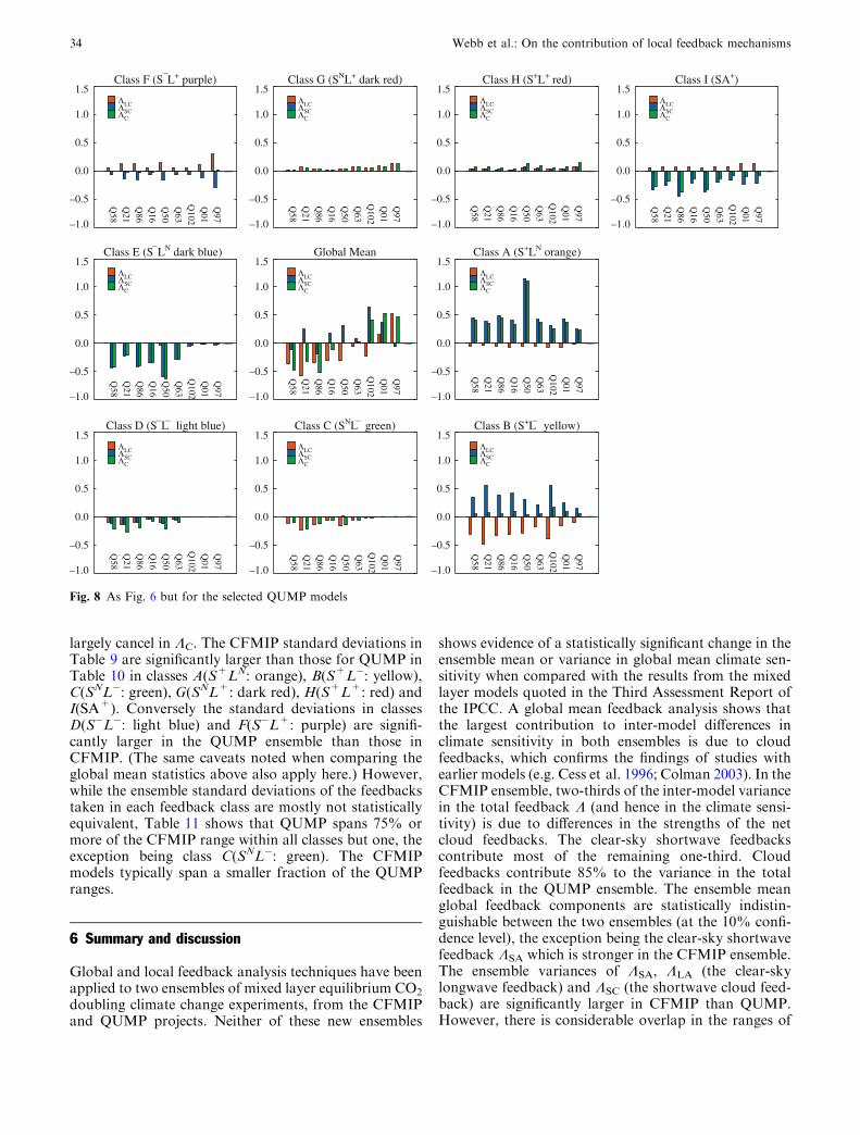
largely cancel in KC. The CFMIP standard deviations inTable 9 are significantly larger than those for QUMP inTable 10 in classes A(S+LN: orange), B(S+L�: yellow),C(SNL�: green), G(SNL+: dark red), H(S+L+: red) andI(SA+). Conversely the standard deviations in classesD(S�L�: light blue) and F(S�L+: purple) are signifi-cantly larger in the QUMP ensemble than those inCFMIP. (The same caveats noted when comparing theglobal mean statistics above also apply here.) However,while the ensemble standard deviations of the feedbackstaken in each feedback class are mostly not statisticallyequivalent, Table 11 shows that QUMP spans 75% ormore of the CFMIP range within all classes but one, theexception being class C(SNL�: green). The CFMIPmodels typically span a smaller fraction of the QUMPranges.

6 Summary and discussion

Global and local feedback analysis techniques have beenapplied to two ensembles of mixed layer equilibrium CO2

doubling climate change experiments, from the CFMIPand QUMP projects. Neither of these new ensembles

shows evidence of a statistically significant change in theensemble mean or variance in global mean climate sen-sitivity when compared with the results from the mixedlayer models quoted in the Third Assessment Report ofthe IPCC. A global mean feedback analysis shows thatthe largest contribution to inter-model differences inclimate sensitivity in both ensembles is due to cloudfeedbacks, which confirms the findings of studies withearlier models (e.g. Cess et al. 1996; Colman 2003). In theCFMIP ensemble, two-thirds of the inter-model variancein the total feedback K (and hence in the climate sensi-tivity) is due to differences in the strengths of the netcloud feedbacks. The clear-sky shortwave feedbackscontribute most of the remaining one-third. Cloudfeedbacks contribute 85% to the variance in the totalfeedback in the QUMP ensemble. The ensemble meanglobal feedback components are statistically indistin-guishable between the two ensembles (at the 10% confi-dence level), the exception being the clear-sky shortwavefeedback KSA which is stronger in the CFMIP ensemble.The ensemble variances of KSA, KLA (the clear-skylongwave feedback) and KSC (the shortwave cloud feed-back) are significantly larger in CFMIP than QUMP.However, there is considerable overlap in the ranges of


–1.0

–0.5

0.0

0.5

1.0

1.5

Q58

Q21

Q86

Q16

Q50

Q63

Q102

Q01

Q97

Q58

Q21

Q86

Q16

Q50

Q63

Q102

Q01

Q97

Q58

Q21

Q86

Q16

Q50

Q63

Q102

Q01

Q97

Q58

Q21

Q86

Q16

Q50

Q63

Q102

Q01

Q97

Q58

Q21

Q86

Q16

Q50

Q63

Q102

Q01

Q97

Q58

Q21

Q86

Q16

Q50

Q63

Q102

Q01

Q97

Q58

Q21

Q86

Q16

Q50

Q63

Q102

Q01

Q97

Q58

Q21

Q86

Q16

Q50

Q63

Q102

Q01

Q97

Q58

Q21

Q86

Q16

Q50

Q63

Q102

Q01

Q97

Q58

Q21

Q86

Q16

Q50

Q63

Q102

Q01

Q97

ΛLCΛSCΛC


–1.0

–0.5

0.0

0.5

1.0

1.5ΛLCΛSCΛC


–1.0

–0.5

0.0

0.5

1.0

1.5ΛLCΛSCΛC


–1.0

–0.5

0.0

0.5

1.0

1.5ΛLCΛSCΛC

Global Mean

–1.0

–0.5

0.0

0.5

1.0

1.5ΛLCΛSCΛC

Class C (SNL green)

–1.0

–0.5

0.0

0.5

1.0

1.5ΛLCΛSCΛC

Class H (S+L+ red)

–1.0

–0.5

0.0

0.5

1.0

1.5ΛLCΛSCΛC


–1.0

–0.5

0.0

0.5

1.0

1.5ΛLCΛSCΛC


–1.0

–0.5

0.0

0.5

1.0

1.5ΛLCΛSCΛC

Class I (SA+)

–1.0

–0.5

0.0

0.5

1.0

1.5ΛLCΛSCΛC

–

–

– – – –

Fig. 8 As Fig. 6 but for the selected QUMP models


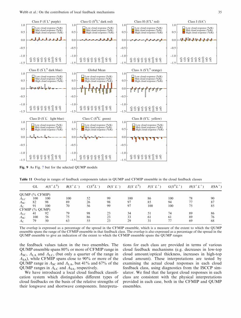
the feedback values taken in the two ensembles. TheQUMP ensemble spans 80% or more of CFMIP range inKSC, KLA and KLC, (but only a quarter of the range inKSA), while CFMIP spans close to 90% or more of theQUMP range in KSC and KLA, but 41% and 67% of theQUMP ranges in KLC and KSA, respectively.

We have introduced a local cloud feedback classifi-cation system which distinguishes different types ofcloud feedbacks on the basis of the relative strengths oftheir longwave and shortwave components. Interpreta-

tions for each class are provided in terms of variouscloud feedback mechanisms (e.g. decreases in low-topcloud amount/optical thickness, increases in high-topcloud amount). These interpretations are tested byexamining the actual cloud responses in each cloudfeedback class, using diagnostics from the ISCCP sim-ulator. We find that the largest cloud responses in eachclass are consistent with the physical interpretationsprovided in each case, both in the CFMIP and QUMPensembles.


–1.5

–1.0

–0.5

0.0

0.5

1.0

Q58

Q21

Q86

Q16

Q50

Q63

Q102

Q01

Q97

Q58

Q21

Q86

Q16

Q50

Q63

Q102

Q01

Q97

Q58

Q21

Q86

Q16

Q50

Q63

Q102

Q01

Q97

Q58

Q21

Q86

Q16

Q50

Q63

Q102

Q01

Q97

Q58

Q21

Q86

Q16

Q50

Q63

Q102

Q01

Q97

Q58

Q21

Q86

Q16

Q50

Q63

Q102

Q01

Q97

Q58

Q21

Q86

Q16

Q50

Q63

Q102

Q01

Q97

Q58

Q21

Q86

Q16

Q50

Q63

Q102

Q01

Q97

Q58

Q21

Q86

Q16

Q50

Q63

Q102

Q01

Q97

Q58

Q21

Q86

Q16

Q50

Q63

Q102

Q01

Q97



–1.5

–1.0

–0.5

0.0

0.5

1.0Low cloud response (%/K)Mid cloud response (%/K)High cloud response (%/K)


–1.5

–1.0

–0.5

0.0

0.5



–1.5

–1.0

–0.5

0.0

0.5


Global Mean

–1.5

–1.0

–0.5

0.0

0.5


Class C (SNL green)

–1.5

–1.0

–0.5

0.0

0.5


Class H (S+L+ red)

–1.5

–1.0

–0.5

0.0

0.5



–1.5

–1.0

–0.5

0.0

0.5



–1.5

–1.0

–0.5

0.0

0.5


Class I (SA+)

–1.5

–1.0

–0.5

0.0

0.5


––– –

–

–

Fig. 9 As Fig. 7 but for the selected QUMP models

Table 11 Overlap in ranges of feedback components taken in QUMP and CFMIP ensemble in the cloud feedback classes


QUMP (% CFMIP)KLC 100 100 100 52 99 100 86 100 78 90KSC 82 98 89 26 98 97 85 94 77 87KC 91 100 70 56 99 97 100 100 75 85CFMIP (% QUMP)KLC 41 92 79 98 23 34 51 74 89 86KSC 100 56 75 86 23 33 61 61 89 76KC 79 50 63 55 23 29 31 77 69 68

The overlap is expressed as a percentage of the spread in the CFMIP ensemble, which is a measure of the extent to which the QUMPensemble spans the range of the CFMIP ensemble in that feedback class. The overlap is also expressed as a percentage of the spread in theQUMP ensemble to give an indication of the extent to which the CFMIP ensemble spans the QUMP ranges


In the CFMIP models, decomposition of the globalfeedback parameters into contributions from the differ-ent cloud feedback classes shows that classes A(S+LN:orange), E(S�LN: dark blue) and I(SA+) (those in whichlow cloud changes constitute the primary cloudresponse) are responsible for 59% of the contribution ofinter-model differences in the net cloud feedback to thevariance in the total feedback. Areas where the short-wave cloud feedback is positive and the longwave cloudfeedback is (relatively) small [class A(S+LN: orange)] areresponsible for most of this contribution (53%). Theseareas coincide with regions of the globe commonlyassociated with the presence of low-top clouds, e.g.along the eastern sides of the tropical ocean basins andin the mid-latitude storm track regions, and the largestcloud responses within them are found to be primarilydue to reductions in low-top cloud amount (althoughreductions in mid-level cloud make a secondary contri-bution). The inter-model differences in the contributionfrom this feedback class are almost entirely due to lowcloud feedback operating over increasingly large areas inthe higher sensitivity models, rather than differences inlocal feedback strengths within the class. Areas wherethe shortwave cloud feedback is negative and the long-wave equivalent is relatively small [class E (S�LN: darkblue)] contribute 18%, and are associated with increasesin the optical thickness of low-top clouds. In the tropicsthis class is commonly seen in the trade cumulus regions,(e.g. to the west of South America), and the oppositesign of the cloud feedback here (compared to that inclass A(S+LN: orange) closer to the coasts) may reflectdiffering cloud feedback processes taking place in con-vectively and turbulently mixed boundary layers. ClassI(SA+) represents areas of non-negligible clear-skyalbedo feedback, in which the ‘cloud radiative forcing’measure of local shortwave cloud feedback requirescareful interpretation. Increases in low cloud amountand optical thickness are seen in these areas which areconsistent with those in classes which show a negativelow cloud feedback in other areas. In the CFMIPensemble this class acts to reduce the contribution ofinter-model differences in cloud feedback to the variancein the total feedback by 12%. The equivalent contribu-tion from classes in which the high-top cloud responsesare strongest [classes B(S+L�: yellow), C(SNL�: green),F(S�L+: purple) and G(SNL+: dark red)] is consider-ably smaller than the low-top total (33% compared with59%). Classes D(S�L�: light blue) and H(S+L+: red)which are due to a combination of low- and high-topcloud changes contribute 8%.

In the QUMP ensemble, the three low-top cloudfeedback classes [A(S+LN: orange), E(S�LN: dark blue)and I(SA+)] are responsible for 59% of the contributionfrom the net cloud feedback to the variance in the totalfeedback (in close agreement with the CFMIP ensem-ble). However, it is class E(S�LN: dark blue) that isresponsible for the largest part of this (39%), while classA(S+LN: orange) (which was largest in CFMIP) makesa small contribution (�1%). Class I(SA+) contributes

21% compared with a negative contribution in CFMIP.As in the CFMIP ensemble, these classes are responsiblefor a larger proportion than the high-top cloud feedbackclasses which contribute 20% in total, or that from theremaining classes (21%).

Bony and Dufresne (2005) examine 1% compoundCO2 coupled climate change experiments from the IPCCAR4 models in the tropics. They find that the radiativeresponse of clouds to changes in surface temperaturesunder climate change in the models differs most inregimes of large scale subsidence, and suggest thatchanges in marine boundary layer clouds are responsi-ble. Our results confirm this by providing direct evidenceof considerable low-top cloud responses in areas whichcontribute most to inter-model differences in globalcloud feedback and climate sensitivity, in both theCFMIP and QUMP ensembles.

We also find evidence of increases in low-top cloudamount and optical depth in high latitude areas where itis difficult to separate the effects of cloud and clear-skyalbedo feedbacks. The application of PRP techniques todiagnose local feedbacks would enable a a cleaner sep-aration of these feedbacks, but it is unlikely that thesewill be applied consistently across all models in theforeseeable future. The evaluation and application ofapproximate PRP methods (e.g. Taylor et al. 2000;Yokohata et al. 2005; Soden and Held 2005) to localfeedback analysis in the CFMIP and QUMP ensembleswill be a subject of future study.

The ensemble mean values of the net cloud feedbacksin seven of the cloud feedback classes are statisticallyindistinguishable between the two ensembles, whileclasses E(S�LN: dark blue) and I(SA+) show significantdifferences (at the 10% confidence level). Standarddeviations are significantly larger in CFMIP comparedto QUMP in six out of nine classes, the exceptions beingclasses D(S�L�: light blue) and F(S�L+: purple) whereQUMP is larger, and class E(S�LN: dark blue) wherethere is no significant difference. However, QUMP spans75% or more of the CFMIP range within all classesexcept class C(SNL�: green), while the CFMIP modelstypically span a smaller fraction of the QUMP ranges ineach class. Given the differences in the statistics of thelocal cloud feedbacks in the two ensembles, it is to beexpected that there will also be differences in the rangesof regional surface temperature responses seen inQUMP compared to those from multi-model ensembles.This does not necessarily mean, however, that theCFMIP local feedbacks and temperature responses areany more or less realistic than those in the QUMPensemble. Further work is required not only to establishthe reasons for these differences, but also to find ways tointegrate the complementary information on uncertaintyprovided by multi-model- and parameter-perturbedensembles. In future probabilistic predictions from theQUMP project we plan to use information from theCFMIP models to include an estimate of the uncertaintyin a prediction which is not represented because ofstructural constraints that may arise from the use of a


single model. See Craig et al. (2001) for an example ofthis approach applied in a different field.

The extent to which we can quantify our confidencein the climate predictions from models is a subject ofongoing study. Confidence measures such as thoseapplied in Murphy et al. (2004) could in principle beapplied to multi-model ensembles as well as perturbedphysics ensembles, but it would be beneficial also toinclude measures that have been shown to be directlyrelevant to the simulation of climate feedbacks (e.g. as inWilliams et al. 2005a, b; Bony and Dufresne 2005). It isinteresting to note that the six model versions in the mid-upper climate sensitivity range of the CFMIP ensembleall have statistical cloud schemes based on either Smith(1990) or Le Treut and Li (1991) (schemes whichthemselves have a common heritage). The next phase ofthe CFMIP project will involve examination of 5 yearsof daily cloud diagnostics from high and low sensitivityCFMIP models in an attempt to understand the differingfeedback processes in terms of the physical assumptionson the models. The Atmospheric Radiation Measure-ment (ARM) and Gewex Cloud System Study (GCSS;Randall et al. 2003) programmes apply a wealth oftechniques to evaluate cloud parametrisations usingregional models, single column models, cloud/eddyresolving models, in situ measurements, operationalanalyses and satellite data (e.g. Xie et al. 2005). Dailycloud diagnostics which capture the key cloud feedbacksin climate models will allow us to apply such techniquesmore directly to evaluating cloud climate feedbackprocesses.

Acknowledgements This work was funded in part by the UKDepartment of the Environment, Food and Rural Affairs, undercontract PECD 7/12/37. Thanks are due also to IPSL for hosting ofCFMIP data, to Jean-Louis Dufresne for providing the IPSLradiative forcing calculations, and to Mat Collins, James Murphyand Jonathan Gregory for helpful comments on the manuscript.We are also grateful to the anonymous reviewers whose commentsled to improvements in this piece of work.

References

Andronova NG, Rozanov EV, Yang F, Schlesinger ME, Stenchi-kov GL (1999) Radiative forcing by volcanic aerosols from1850 through 1994. J Geophys Res 104:807–816

Boer GJ, Yu B (2003) Climate sensitivity and response. Clim Dyn20:415–429

Bony S, Dufresne J-L (2005) Marine boundary layer clouds at theheart of tropical cloud feedback uncertainties in climate models.Geophys Res Lett 32:L20806. DOI 10.1029/2005GL023851

Bony S, Emanuel KA (2001) A parameterization of the cloudinessassociated with cumulus convection; evaluation using TOGACOARE data. J Atmos Sci 58:3158–3183

Bony S, Dufresne JL, Le Treut H, Morcrette JJ, Senior CA (2004)On dynamic and thermodynamic components of cloud changes.Clim Dyn 22:71–86 DOI 10.1007/s00382-003-0369-6

Cess RD, Potter GL (1988) A methodology for understanding andintercomparing atmospheric climate feedback processes ingeneral circulation models. J Geophys Res 93:8305–8314

Cess RD, Potter GL, Blanchet JP, Boer GJ, Del Genio AD, DequeM, Dymnikov V, Galin V, Gates WL, Ghan SJ, Kiehl JT, LacisAA, Le Treut H, Li ZX, Liang XZ, Macavaney BJ, Meleshko

VP, Mitchell JFB, Morcrette J-J, Randall DA, Rikus L, Roe-ckner E, Royer JF, Schelse U, Scheinin DA, Slingo A, SokolovAP, Taylor KE, Washington WM, Wetherald RT, Yagai I,Zhang MH (1990) Intercomparison and interpretation of cli-mate feedback processes in 19 atmospheric general circulationmodels. J Geophys Res 95:16601–16615

Cess RD, Zhang MH, Ingram WJ, Potter GL, Alekseev V, BarkerHW, Cohen-Solal E, Colman RA, Dazlich DA, Del Genio AD,Dix MR, Dymnikov V, Esch M, Fowler LD, Fraser JR, GalinV, Gates WL, Hack JJ, Kiehl JT, Treut HL, Lo KKW,McAvaney BJ, Meleshko VP, Morcrette JJ, Randall DA,Roeckner E, Royer JF, Schlesinger ME, Sporyshev PV, TimbalB, Volodin EM, Taylor KE, Wang W, Wetherald RT (1996)Cloud feedback in atmospheric general circulation models: Anupdate. J Geophys Res 101:12791–12794

Colman R (2002) Geographical contributions to global climatesensitivity in a general circulation model. Global Planet Change32:211–243

Colman R (2003) A comparison of climate feedbacks in generalcirculation models. Clim Dyn 20:865–873

Colman R, Fraser J, Rotstayn L (2001) Climate feedbacks in ageneral circulation model incorporating prognostic clouds.Clim Dyn 18:103–122

Craig PM, Goldstein M, Rougier J, Sehueult A (2001) Bayesianforecasting for complex systems using computer simulators. JAm Stat Assoc 96:717–729

Cubasch U, Meehl GA, Boer GJ, Stouffer RJ, Dix M, Noda A,Senior CA, Raper SCB, Yap KS (2001) Projections of futureclimate change. In: Houghton JT, Ding Y, Griggs DJ, NoguerM, van der Linden P, Dai X, Maskell K, Johnson CI (eds)Climate change 2001: the scientific basis. Contribution ofWorking Group I to the Third Assessment Report of theIntergovernmental Panel on Climate Change. Cambridge Uni-versity Press, London, pp 525–582

Delworth TL, Broccoli AJ, Rosati A, Stouffer RJ, Balaji V, BeesleyJT, Cooke WF, Dixon KW, Dunne J, Dunne KA, DurachtaJW, Findell KL, Ginoux P, Gnanadesikan A, Gordon CT,Griffies SM, Gudgel R, Harrison MJ, Held IM, Hemler RS,Horowitz LW, Klein SA, Knutson TR, Kushner PJ, Langen-horst AR, Lee H-C, Lin S-J, Lu J, Malyshev SL, Milly PC D,Ramaswamy V, Russell J, Schwarzkopf MD, Shevliakova E,Sirutis JJ, Spelman MJ, Stern WF, Winton M, Wittenberg AT,Wyman B, Zeng F and Zhang R (2006). GFDL’s CM2 GlobalCoupled Climate Models—Part 1: Formulation and simulationcharacteristics. J Climate (in press)

GFDL Global Atmospheric Model Development Team (GAMDT)(2004) The new GFDL global atmosphere and land modelAM2–LM2: evaluation with prescribed SST simulations.J Climate 17(24):4641–4673

Hansen J, SatoM, Nazarenko L, Ruedy R, Lacis A, Koch D, TegenI, Hall T, Shindell D, Santer B, Stone P, Novakov T, ThomasonL, Wang R, Wang Y, Jacob D, Hollandsworth-Frith S, BishopL, Logan J, Thompson A, Stolarski R, Lean J, Willson R,Levitus S, Antonov J, Rayner N, Parker D, Christy J (2002)Climate forcings in Goddard Institute for Space Studies SI2000simulations. J Geophys Res 107. DOI 10.1029/2001JD001143

Hourdin F, Musat I, Bony S, Braconnot P, Codron, F, DufresneJ-L, Fairhead L, Filiberti M-A, Friedlingstein P, Grandpeix J,Krinner G, LeVan P, Li Z-X, Lott F (2006) The LMDZ generalcirculation model: climate performance and sensitivity toparameterized physics with emphasis on tropical convection.Clim Dyn (in revision)

Johns TC, Durman CF, Banks HT, Roberts MJ, McLaren AJ,Ridley JK, Senior CA, Williams KD, Jones A, Coauthors(2006) The new Hadley Centre climate model HadGEM1:evaluation of coupled simulations in comparison to previousmodels. J Climate (in press)

Joshi M, Shine K, Ponater M, Stuber N, Sausen R, Li L (2003) Acomparison of climate response to different radiative forcings inthree general circulation models: towards an improved metric ofclimate change. Clim Dyn 20:843–854. DOI 10.1007/s00382-003-0305-9


K-1 model developers (2004) K-1 coupled model (MIROC)description. In: Hasumi H, Emori S (eds) K-1 technical report,1. Center for Climate System Research, University of Tokyo,Tokyo, 34 pp (available from http://www.ccsr.u-tokyo.ac.jp/kyosei/hasumi/MIROC/tech-repo.pdf)

Klein SA, Jakob C (1999) Validation and sensitivities of frontalclouds simulated by the ECMWF model. Mon Weather Rev127(10):2514–2531

Le Treut H, Li ZX (1991) Sensitivity of an atmospheric generalcirculation model to prescribed SST changes: feedback effectsassociated with the simulation of cloud optical properties. ClimDyn 5:175–187

Le Treut H, McAvaney B (2000) Equilibrium climate change inresponse to a CO2 doubling: an intercomparison of AGCMsimulations coupled to slab oceans. Technical Report, InstitutPierre Simon Laplace 18:20

Martin GM, Ringer MA, Pope VD, Jones A, Dearden C, Hinton T(2005) The physical properties of the atmosphere in the newHadley Centre Global Environmental Model, HadGEM1. Part1: Model description and global climatology. J Climate(in press)

McAvaney BJ, Le Treut H (2003) The cloud feedback intercom-parison project: (CFMIP). In: CLIVAR Exchanges—supple-mentary contributions. 26:March

Murphy JM, Sexton DMH, Barnett DN, Jones GS, Webb MJ,Collins M, Stainforth DA (2004) Quantification of modellinguncertainties in a large ensemble of climate change simulations.Nature 430:768–772

Pope VD, Gallani ML, Rowntree PR, Stratton RA (2000) Theimpact of new physical parametrizations in the Hadley Centreclimate model—HadAM3. Clim Dyn 16:123–146

Randall D, Krueger S, Bretherton C, Curry J, Duynkerke P,Moncrieff M, Ryan B, Starr D, Miller M, Rossow W, Tse-lioudis G, Wielicki B (2003) Confronting models with data—theGEWEX cloud systems study. Bull Am Meteorol Soc 84:455–469

Rossow WB, Schiffer RA (1999) Advances in understanding cloudsfrom ISCCP. Bull Am Meteorol Soc 80:2261–2287

Rotstayn LD (1997) A physically based scheme for the treatment ofstratiform clouds and precipitation in large-scale models. Part1: Description and evaluation of the microphysical processes.Q J R Meteorol Soc 123:1227–1282

Senior CA, Mitchell JFB (1993) Carbon dioxide and climate: theimpact of cloud parameterization. J Clim 6:393–418

Sexton DMH, Collins M, Harris G, Murphy JM, Webb MJ (2004)Improvements in sampling parameter space for probabilisticclimate predictions. DEFRA Report (available on request fromthe Hadley Centre)

Smith RNB (1990) A scheme for predicting layer clouds and theirwater content in a general circulation model. Q J R MeteorolSoc 116:435–460

Soden BJ, Held IM (2005) An assessment of climate feedbacks incoupled ocean-atmosphere models. J Climate (in revision)

Soden BJ, Broccoli AJ, Hemler RS (2004) On the use of cloudforcing to estimate cloud feedback. J Climate 17(19):3661–3665.DOI 10.1175/1520-0442(2004)017

Stainforth DA, Aina T, Christensen C, Collins M, Frame DJ,Kettleborough JA, Knight S, Martin A, Murphy J, Piani C,Sexton D, Smith LA, Spicer RA, Thorpe AJ, Allen MR (2005)Uncertainty in predictions of the climate response to risinglevels of greenhouse gases. Nature 433:403–406

Taylor KE, Hewitt CD, Braconnot P, Broccoli AJ, Doutriaux C,Mitchell JFB (2000) Analysis of forcing, response and feed-backs in a paleoclimate modeling experiment PMIP, 2000:Paleoclimate Modelling Intercomparison Project (PMIP). In:

Braconnot P (eds) Proceedings of the third PMIP workshop,Canada, 4–8 October 1999, WCRP Report WCRP-111, WMO/TD-No. 1007, pp 43–49

Tett SFB, Jones GS, Stott PA, Hill DC, Mitchell JFB, Allen MR,Ingram WJ, Johns TC, Johnson CE, Jones A, Roberts DL,Sexton DMH, Woodage MJ (2002) Estimation of natural andanthropogenic contributions to 20th century temperaturechange. J Geophys Res 107. DOI 10.1029/2000JD000028

Tselioudis G, Zhang Y, Rossow WB (2000) Cloud and radiationvariations associated with northern midlatitude low and highsea level pressure regimes. J Climate 13(2):312–327

Webb M, Senior C, Bony S, Morcrette JJ (2001) Combining ERBEand ISCCP data to assess clouds in the Hadley Centre,ECMWF and LMD atmospheric climate models. Clim Dyn17:905–922

Wetherald RT, Manabe S (1988) Cloud feedback processes in ageneral circulation model. J Atmos Sci 45:1397–1415

Williams KD, Jones A, Roberts DL, Senior CA, Woodage MJ(2001a) The response of the climate system to the indirect effectsof anthropogenic sulfate aerosol. Clim Dyn 17:845–856

Williams KD, Senior CA, Mitchell JFB (2001b) Transient climatechange in the Hadley Centre models: the role of physical pro-cesses. J Climate 14(12):2659–2674

Williams KD, Ringer MA, Senior CA (2003) Evaluating the cloudresponse to climate change and current climate variability. ClimDyn 20:705–721. DOI 10.1007/s00382-002-0303-3

Williams KD, Ringer MA, Senior CA, Webb MJ, McAvaney BJ,Andronova N, Bony S, Dufresne J-L, Emori S, Gudgel R,Knutson T, Li B, Lo K, Musat I, Wegner J, Slingo A, MitchellJFB (2005a) Evaluation of a component of the cloud responseto climate change in an intercomparison of climate models.Clim Dyn DOI:10.1007/s00382-005-0067-7

Williams KD, Senior CA, Slingo A, Mitchell JFB (2005b) Towardsevaluating cloud response to climate change using clusteringtechnique identification of cloud regimes. Clim Dyn 24:701–719

Wilson DR, Ballard SP (1999) A microphysically based precipita-tion scheme for the UK Meteorological Office Unified Model.Q J R Meteorol Soc 125:1607–1636

Xie S, Zhang M, Branson M, Cederwall RT, Del Genio AD, EitzenZA, Ghan SJ, Iacobellis SF, Johnson KL, Khairoutdinov M,Klein SA, Krueger SK, Lin W, Lohmann U, Miller MA,Randall DA, Somerville RCJ, Sud YC, Walker GK, Wolf A,Wu X, Xu K-M, Yio JJ, Zhang G, Zhang JH (2005) Simula-tions of midlatitude frontal clouds by single-column andcloud-resolving models during the Atmospheric RadiationMeasurement March 2000 cloud intensive operational period. JGeophys Res 110(D15S03). DOI 10.1029/2004JD005119

Yang F, Schlesinger ME, Rozanov EV (2000) Description and per-formance of the UIUC 24-layer stratosphere-troposphere gen-eral-circulation model. J Geophys Res 105(D14):17925–17954

Yokohata T, Emori S, Nozawa T, Tsushima Y, Ogura T, KimotoM (2005) A simple scheme for climate feedback analysis.Geophys Res Lett 32:L19703

Yu W, Doutriaux M, Seze G, Le Treut H, Desbois M (1996) Amethodology study of the validation of clouds in GCMs usingISCCP satellite observations. Clim Dyn 12:389–401

Zhang MH, Cess RD, Hack JJ, Kiehl JT (1994) Diagnostic studyof climate feedback processes in atmospheric GCMs. J GeophysRes 99:5525–5537

Zhang MH, Lin WY, Klein SA, Bacmeister JT, Bony S, CederwallRT, Del Genio AD, Hack JJ, Loeb NG, Lohmann U, Minnis P,Musat I, Pincus R, Stier P, Suarez MJ, Webb MJ, Wu JB (2005)Comparing clouds and their seasonal variations in 10 atmo-spheric general circulation models with satellite measurements.J Geophys Res 110(D15)


Documents

On the contribution of local feedback mechanisms to the ... · PDF fileAbstract Global and local feedback ... (Cloud Feedback Model Intercom-parison Project) and QUMP (Quantifying